PERFORMANCE MODELS FOR DISTRIBUTED-MEMORY A Thesis

PERFORMANCE MODELS FOR DISTRIBUTED-MEMORY

HPC SYSTEMS AND DEEP NEURAL NETWORKS

A Thesis

Submitted to the Faculty

of

Purdue University

by

David Cardwell

In Partial Fulfillment of the

Requirements for the Degree

of

Master of Science

December 2019

Purdue University

Indianapolis, Indiana

ii

THE PURDUE UNIVERSITY GRADUATE SCHOOL

STATEMENT OF THESIS APPROVAL

Dr. Fengguang Song, Chair

Department of Computer and Information Science

Dr. Snehasis Mukhopadhyay


Dr. Mihran Tuceryan


Approved by:

Dr. Shiaofen Fang

Head of the Graduate Program

iii

ACKNOWLEDGMENTS

I would like to thank Professor Song for his guidance in preparing this thesis.

iv

TABLE OF CONTENTS

Page

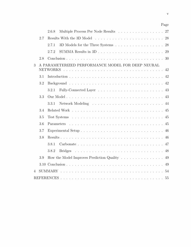
LIST OF TABLES . . . . . . . . . . . . . . . . . . . . . . . . . . . . . . . . . . vi

LIST OF FIGURES . . . . . . . . . . . . . . . . . . . . . . . . . . . . . . . . . vii

ABSTRACT . . . . . . . . . . . . . . . . . . . . . . . . . . . . . . . . . . . . . viii

1 INTRODUCTION . . . . . . . . . . . . . . . . . . . . . . . . . . . . . . . . 1

2 AN EXTENDED ROOFINE MODEL WITH COMMUNICATION-AWARENESS 4

2.1 Introduction . . . . . . . . . . . . . . . . . . . . . . . . . . . . . . . . . 4

2.2 Background . . . . . . . . . . . . . . . . . . . . . . . . . . . . . . . . . 7

2.3 An Extended New Roofline Model . . . . . . . . . . . . . . . . . . . . . 8

2.3.1 Limitations of the Model . . . . . . . . . . . . . . . . . . . . . . 10

2.3.2 Changed Aspects With Respect to the Original Roofline Model 10

2.3.3 Determining the Model Parameters . . . . . . . . . . . . . . . . 11

2.3.4 Visualizing the New Model in 3D . . . . . . . . . . . . . . . . . 14

2.4 Related Work . . . . . . . . . . . . . . . . . . . . . . . . . . . . . . . . 15

2.4.1 Roofline Model Extensions . . . . . . . . . . . . . . . . . . . . . 15

2.4.2 Research Related to Communication Models . . . . . . . . . . . 16

2.5 Applications . . . . . . . . . . . . . . . . . . . . . . . . . . . . . . . . . 17

2.6 Experimental Results . . . . . . . . . . . . . . . . . . . . . . . . . . . . 20

2.6.1 Experimental Setup . . . . . . . . . . . . . . . . . . . . . . . . . 20

2.6.2 Comparing With the Original Roofline Model Quantitatively . . 21

2.6.3 Interpreting the Figures . . . . . . . . . . . . . . . . . . . . . . 22

2.6.4 Results for the Seven Algorithms . . . . . . . . . . . . . . . . . 24

2.6.5 Vector Dot Product . . . . . . . . . . . . . . . . . . . . . . . . . 27

2.6.6 Matrix-Vector Product . . . . . . . . . . . . . . . . . . . . . . . 27

2.6.7 Dijkstra’s Algorithm . . . . . . . . . . . . . . . . . . . . . . . . 27

v

Page

2.6.8 Multiple Process Per Node Results . . . . . . . . . . . . . . . . 27

2.7 Results With the 3D Model . . . . . . . . . . . . . . . . . . . . . . . . 28

2.7.1 3D Models for the Three Systems . . . . . . . . . . . . . . . . . 28

2.7.2 SUMMA Results in 3D . . . . . . . . . . . . . . . . . . . . . . . 29

2.8 Conclusion . . . . . . . . . . . . . . . . . . . . . . . . . . . . . . . . . . 30

3 A PARAMETERIZED PERFORMANCE MODEL FOR DEEP NEURALNETWORKS . . . . . . . . . . . . . . . . . . . . . . . . . . . . . . . . . . . 42

3.1 Introduction . . . . . . . . . . . . . . . . . . . . . . . . . . . . . . . . . 42

3.2 Background . . . . . . . . . . . . . . . . . . . . . . . . . . . . . . . . . 42

3.2.1 Fully-Connected Layer . . . . . . . . . . . . . . . . . . . . . . . 43

3.3 Our Model . . . . . . . . . . . . . . . . . . . . . . . . . . . . . . . . . . 43

3.3.1 Network Modeling . . . . . . . . . . . . . . . . . . . . . . . . . 44

3.4 Related Work . . . . . . . . . . . . . . . . . . . . . . . . . . . . . . . . 45

3.5 Test Systems . . . . . . . . . . . . . . . . . . . . . . . . . . . . . . . . 45

3.6 Parameters . . . . . . . . . . . . . . . . . . . . . . . . . . . . . . . . . 45

3.7 Experimental Setup . . . . . . . . . . . . . . . . . . . . . . . . . . . . . 46

3.8 Results . . . . . . . . . . . . . . . . . . . . . . . . . . . . . . . . . . . . 46

3.8.1 Carbonate . . . . . . . . . . . . . . . . . . . . . . . . . . . . . . 47

3.8.2 Bridges . . . . . . . . . . . . . . . . . . . . . . . . . . . . . . . 48

3.9 How the Model Improves Prediction Quality . . . . . . . . . . . . . . . 49

3.10 Conclusion . . . . . . . . . . . . . . . . . . . . . . . . . . . . . . . . . . 49

4 SUMMARY . . . . . . . . . . . . . . . . . . . . . . . . . . . . . . . . . . . . 54

REFERENCES . . . . . . . . . . . . . . . . . . . . . . . . . . . . . . . . . . . . 55

vi

LIST OF TABLES

Table Page

2.1 The tested systems and their specifications. . . . . . . . . . . . . . . . . . 7

2.2 A summary of the five parameters of the model. . . . . . . . . . . . . . . . 12

2.3 The benchmark results for the system-specific parameters for our threesystems. . . . . . . . . . . . . . . . . . . . . . . . . . . . . . . . . . . . . 13

2.4 Our derived operational intensity and communication arithmetic intensityformulas used in our models. . . . . . . . . . . . . . . . . . . . . . . . . . . 19

2.5 The tested problem sizes for each algorithm and system. . . . . . . . . . . 20

2.6 We display the difference between the original Roofline model and ours inthis table. . . . . . . . . . . . . . . . . . . . . . . . . . . . . . . . . . . . . 23

3.1 The layer weight sizes and output sizes for the simple network. . . . . . . . 44

3.2 The tested systems and their specifications. . . . . . . . . . . . . . . . . . 46

3.3 Microbenchmark results for Carbonate. . . . . . . . . . . . . . . . . . . . . 47

3.4 Microbenchmark results for Bridges. . . . . . . . . . . . . . . . . . . . . . 48

3.5 The meaning of each column in the result graphs. . . . . . . . . . . . . . . 49

3.6 Results for the simple network on Carbonate. . . . . . . . . . . . . . . . . 50

3.7 Results for the simple network on Bridges. . . . . . . . . . . . . . . . . . 53

3.8 A summary of the results using MAPE. . . . . . . . . . . . . . . . . . . . . 53

vii

LIST OF FIGURES

Figure Page

2.1 An example of the original Roofline model for the Karst computer system 5

2.2 a) This visualization shows the operational intensity graph for the new model 9

2.3 Here we show the 2D visualization of the new model . . . . . . . . . . . . 31

2.4 Here we display the ratio of communication for the computer systems andalgorithms . . . . . . . . . . . . . . . . . . . . . . . . . . . . . . . . . . . . 32

2.5 The operational intensity and communication diagrams for FFT . . . . . . 33

2.6 The operational intensity and communication diagrams for Stencil . . . . . 34

2.7 The operational intensity and communication diagrams for MST . . . . . . 35

2.8 The operational intensity and communication diagrams for DDOT . . . . . 36

2.9 The operational intensity and communication diagrams for DGEMV . . . . 37

2.10 The operational intensity and communication diagrams for Dijkstra . . . . 38

2.11 For SUMMA, we display the multi-process results here . . . . . . . . . . . 39

2.12 We can compare the three systems uing the 3D model . . . . . . . . . . . 40

2.13 Results for SUMMA plotted using the 3D visualization . . . . . . . . . . . 41

3.1 Results for the simple network on Carbonate . . . . . . . . . . . . . . . . . 51

3.2 Results for the simple network on Bridges . . . . . . . . . . . . . . . . . . 52

viii

ABSTRACT

Cardwell, David M.S., Purdue University, December 2019. Performance Models forDistributed-Memory HPC Systems And Deep Neural Networks. Major Professor:Fengguang Song.

Performance models are useful as mathematical models to reason about the behav-

ior of different computer systems while running various applications. An additional

purpose is predicting performance without having to run a given application on a

target system. Models that simultaneously provide accurate results as well as insight

in optimization techniques are difficult to develop since more accurate models tend

to be more complex. Straightforward and precise models are of great interest for this

reason.

In this thesis, we aim to provide two distinct performance models: one for distributed-

memory high performance computing systems with network communication, and one

for deep neural networks. Our main goal for the first model is insight and simplicity,

while for the second we aim for accuracy in prediction. The first model is generalized

for networked multi-core computer systems, while the second is specific to deep neural

networks on a shared-memory system.

First, we enhance the well-known Roofline model with extensions to add commu-

nication awareness. To do so, we introduce the concept of communication arithmetic

intensity, which is the network equivalent of operational intensity. In the second

model, we use performance measurements from target systems to parameterize the

model by the problem size. For both models, we performed an empirical analysis on

several target systems with various algorithms and applications to verify the quality

of the predictions.

ix

With our communication-aware extended Roofline model, we improve on the orig-

inal model by up to 100% on all three tested computer systems according to our

MAPE-based comparision method. For the deep neural network model, we attain up

to a 23.43% absolute prediction error.

To our knowledge, our communication-aware Roofline model is the first Roofline

extension to consider communication, while our second model is the first model of

deep neural networks that uses parameterization.

1

1. INTRODUCTION

Performance models are a key part of performance studies and are widely used in

High Performance Computing to predict the runtime efficiency of running various

applications on assorted computer systems. These models allow insight to be gained

on how a program can be optimized or where bottlenecks exist on particular hardware

configurations. This allows implementers to better determine how to increase the

performance of their applications, whether optimizing the code itself or changing the

hardware.

A core issue of performance modeling is the level of complexity of the model.

Generally, more complex models allow for higher prediction accuracy, but this comes

at the cost of the intuitiveness of the model. For example, if the level of abstraction is

low, such as at the level of microarchitectural details such as out-of-order execution,

the model can become difficult to reason about. On the other hand, a model that is

high-level may provide intuition about performance bottlenecks but little efficacy in

prediction. Models that manage to be simple and accurate are of interest since they

solve both concerns. One such model is the Roofline model, which is both simple and

widely-used.

Performance models are of particular interest in High Performance Computing,

where speed of execution and optimization are core goals. Since these systems are

distributed-memory and rely on networks, modeling the interconnect is important

since it is often a bottleneck. In addition, due to the increasing importance of deep

neural networks, performance models for machine learning applications on HPC sys-

tems are of significance. In this thesis we aim to create models for both, providing an

extended Roofline model with support for network communication as well as a model

specialized for deep neural networks.

2

For our extended Roofline model, we take the original model’s concept of opera-

tional intensity and expand it for networked systems with the concept of communi-

cation arithmetic intensity. With this, we can model the speed of the interconnect

in addition to memory bandwidth for improved prediction accuracy on distributed-

memory systems. This model is generalized for all kinds of HPC applications. In the

case of the deep neural network model, we use parameterization of collected perfor-

mance results to predict the execution time. In contrast, this model is highly specific

to a particular computer system and application.

For both models we empirically validate them using target applications and sys-

tems to determine their effectiveness. The purpose of these tests is to thoroughly

determine the prediction quality of the models. For the extended Roofline model, we

tested seven algorithms on three computer systems. These are dense matrix-matrix

product (SUMMA), 1D fast Fourier transform, a 2D 5-point stencil, Boruvka’s min-

imum spanning tree, dense matrix-vector product, and dot product. The computer

systems are Big Red II and Karst at Indiana University, as well as Jetstream from

XSEDE. For the neural network model, we tested two networks on two computer

systems. The first network is a simple network consisting of only fully-connected

layers and activations, and the second network is the widely-known LeNet. The two

computer systems we tested are Bridges at the Pittsburgh Supercomputing Center,

and Carbonate at Indiana University.

The extended Roofline model improves on the original in nearly all cases that we

tested. The best results were achieved for the minimum-spanning-tree algorithm for

all three systems, for a percentage improvement of 100%. For the deep neural network

model, our best results were achieved for particular layers of the LeNet network on

Carbonate and Bridges with an error of 23.43% and 30.24% respectively.

We believe that these two approaches to performance modeling are novel and of

interest to those working with both distributed systems and neural networks. To our

knowledge, the extended Roofline model is the first extension supporting network

communication and the deep neural network model is the first specialized and pa-

3

rameterized model for neural networks. In this sense, we provide both a broad model

for HPC in general, and a highly particular model just for machine learning.

4

2. AN EXTENDED ROOFINE MODEL WITH

COMMUNICATION-AWARENESS

2.1 Introduction

Our first goal is producing a performance model that is intuitive and insightful

with regard to the balance of floating-point computations, memory accesses and com-

munciation costs. This would allow evaluating new computing platforms and parallel

applications. The Roofline model [1] succeeds in being straightforward and easy-to-

understand while giving a picture of the balance of floating-point computation and

memory operations. The model is both simple and flexible, suggesting that extending

it to consider network communication is feasible.

The model is widely used, [2] [3] [4] [5] [6] however, measuring the communication

costs of the network is not of its goals. We seek to produce an extension to consider

the network as a bottleneck as well as the memory and floating-point bottlenecks.

We introduce a new concept, communication arithmetic intensity in order to do this.

Since this is the communication counterpart of operational intensity, we can now

consider all three bottlenecks in a single easy-to-understand visualization. Our model

has two primary advantages, simple input parameters and that it is visual.

The first advantage is that the input parameters are simple. The Roofline model

has a small number of input parameters that are easy to derive or measure. We carry

this over to the new model in order to keep the simplicity. For example, we do not use

the latency of the network, the message size, the message receive overhead, or message

send overhead. Our communication benchmark is a simple ping-pong test [7]. This

benchmark is added to the memory and floating-point benchmarks required by the

original Roofline model.

5

Ridge Point

2

4

8

16

0.25 1.00 4.00 16.00

Operational Intensity (Flops/Byte)

Atta

inab

le G

FLO

PS

/s

Original Roofline Model

Fig. 2.1. An example of the original Roofline model for the Karstcomputer system. The ridge point is emphasized with a red dottedline. When the operational intensity increases beyond this location,maximum performance is achieved.

The second advantage is that it is a visual model. This makes it easy to under-

stand. We have both 2D and 3D visualizations of the model. By having both types

visualizations two or three bottlenecks can be considered at a time. For example,

in the 2D models, we can either visualize the attainable performance vs. the oper-

ational intensity, or the attainable performance vs. the communication arithmetic

intensity. The 3D model shows the attainable performance, operational intensity and

communcation intensity in a single visualization.

Like with the original Roofline model, the ridge point is important to understand-

ing the visualization of our new model. An example can be seen in Fig 2.1, where

6

it is the lowest level of operational intensity that can still achieve the highest possi-

ble performance. Operational intensities below this point cannot achieve maximum

floating-point performance. Since a given algorithm has a particular operational in-

tensity for a particular problem size, we can classify scenarios based on whether they

lie to the left or the right of the ridge point, either memory-bound or CPU-bound.

This allows us to identify the bottleneck and make a performance prediction. To do

this, it is not necessary to run the program on the target hardware. This is true for

both the original Roofline model and our extensions.

For the communication visualization in our new model, the ridge point now iden-

tifies whether an algorithm is communication-bound or compute-bound. If a com-

munication arithmetic intensity lies to the left of the ridge point, the algorithm is

communication-bound. Otherwise, it is compute-bound. By considering this we can

classify algorithms in a simple manner.

To demonstrate the model, we evaluated it on seven parallel algorithms to deter-

mine the quality of the prediction. We used dense matrix-matrix product (SUMMA),

1D fast Fourier transform, a 2D 5-point stencil, Boruvka’s minimum spanning tree,

dense matrix-vector product, and dot product. These algorithms cover three of the

seven motifs of High Performance Computing [8].

We took these algorithms and tested three different HPC systems. Big Red II

represents High Performance Computing, while Karst represents High Throughput

Computing and Jetstream represents Cloud Computing. We list the specifications of

these systems in Table 2.1.

This chapter makes the following contributions:

• We present an extended Roofline model that considers distributed memory sys-

tems with network communication.

• We tested the model with seven algorithms on four computing systems to vali-

date the strength of the prediction. The new model generally achieves a tighter

upper bound compared to the original model.

7

Table 2.1.The tested systems and their specifications.

Big Red II Karst Jetstream

System Type HPC HTC Cloud

Processor Family AMD Opteron Intel Xeon Intel Xeon

Processor Model 6380 E5-2650 E-2680v3

Cores Per Socket 16 8 12

Sockets Per Node 2 2 2

RAM Per Node 64GB 32GB 128GB

Network Gemini 10GbE 10GbE

OS Cray Linux Red Hat 6 CentOS 7

• We analyzed the efficacy of HPC, high-throughput and cloud systems with

regard to these parallel and distributed algorithms.

2.2 Background

The original Roofline model [1] was developed to make a easy-to-understand and

straightforward performance model for multi-threaded systems with shared memory.

Due to its strengths, it has been used widely. Understanding the relationship between

attainable performance and memory bandwidth is difficult, but the Roofline model

makes it easier to comprehend.

Equation 2.1 defines the original Roofline model. The peak memory bandwidth

is multiplied by the operational intensity, and the minimum of that result is taken

with the peak floating-point performance. This gives the attainable floating-point

performance.

Operational intensity, as in Equation 2.2, is then designated as the number of

floating-point operations divided by the memory bytes transferred. This operational

8

intensity ratio will affect whether an algorithm is floating-point-bound or memory-

bound. For example, the BLAS function dgemm has a high operational intensity, which

indicates that it is floating-point-bound, while daxpy has a low operational intensity,

which indicates that it is memory-bound.

Attainable GFLOPS/s = Min(

Peak Floating Point Performance,

Peak Memory Bandwidth×Operational Intensity)

(2.1)

Operational intensity =Floating-point operations

Memory bytes transferred(2.2)

Three examples of original Roofline models are provided in Fig. 2.2-a. The red

line represents Big Red II, while blue represents Jetstream, and green represents

Karst. On the X-axis we have operational intensity, while on the Y-axis we have the

attainable floating-point performance.

2.3 An Extended New Roofline Model

Since the original Roofline model was not developed to consider network com-

munication, we introduce the concept of communication arithmetic intensity. It is

defined by Equation 2.3. The peak communication bandwidth is multiplied by the

communication arithmetic intensity, and the minimum of that result is taken with

the peak floating-point performance. This gives the attainable floating-point perfor-

mance. Compared to the original model, communication bandwidth replaces memory

bandwidth, and communication arithmetic intensity replaces operational intensity.

In the original model, operational intensity uses the memory bytes transferred.

Communication arithmetic intensity is defined as the ratio of floating-point operations

and the network bytes transferred, as can be seen in Equation 2.4. By doing so, we

now have the ratio of network communication to computation the same way the

original model has the ratio of memory bytes to computation.

9

2

4

8

16

32

0.25 1.00 4.00 16.00


Atta

inab

le G

FLO

PS

/sa) Original Roofline Models

0.1

1.0

8.0

0.5 4.0 32.0 256.0

Comm. Arith. Int. (Flops/Net. Byte)

Atta

inab

le G

FLO

PS

/s

b) New Roofline Models

System Big Red II Jetstream Karst

Fig. 2.2. a) This visualization shows the operational intensity graphfor the new model. This is identical to the original Roofline model.The three systems are displayed with three distinct lines, with redfor Big Red II, blue for Jetstream, and green for Karst. b) The com-munication arithmetic intensity graph of our new model. We nowhave communication arithmetic intensity on the X-axis rather thenoperational intensity.

10



Peak Communication Bandwidth× Communication Arithmetic Intensity)

(2.3)

Communication arithmetic intensity =Floating-point operations

Network bytes transferred(2.4)

In this model, the ridge point differentiates between communication-bound and

floating-point-bound algorithms. Applications with a communication arithmetic in-

tensity to the left of the ridge point need to investigate reducing the number of

messages or the size of the messages sent over the network. Otherwise, the algo-

rithm is floating-point-bound and different optimizations need to be investigated.

For memory-bound algorithms, we still use the original Roofline model to differen-

tiate. In this sense, the communication Roofline model complements the original

Roofline model and adds a new dimension. Using both allows discerning memory-

bound, floating-point-bound and communication-bound algorithms.

2.3.1 Limitations of the Model

The original Roofline model simplifies things such as latency and miroarchitec-

tural details to keep the model easy to understand. Similarly, the communication

model considers communication to be synchronous and inter-node. We tested applica-

tions that mostly use synchronous communication operations such as MPI Allgather

rather than asynchronous ones such as MPI Isend. We do not consider latency either,

similarly to how the original model does not consider RAM access latency.

2.3.2 Changed Aspects With Respect to the Original Roofline Model

Some versions of the original Roofline model have additional ceilings in the plot to

differentiate between FMA or SIMD operations, for example. We have not done this

with the communication aspect of the model, and have the communication roofline

11

in a separate plot from the memory roofline. This is done because of the invention of

communication arithmetic intensity. In the original Roofline model, FMA or SIMD

still use operational intensity and the X-axis is the same regardless. In our model,

we use communication arithmetic intensity and the X-axis has changed. Therefore,

we cannot superimpose the communication roofline on the memory roofline and keep

them both in a single chart.

In addition, a single 2D chart would not be able to differentiate between the three

bottlenecks (memory, floating-point, or communication). For this reason, we invented

the 3D visualization of our model. The 2D visualization with two charts side-by-side

can be considered a projection of the 3D one.

2.3.3 Determining the Model Parameters

As the original Roofline model has operational intensity, peak memory bandwidth,

and peak floating-point performance, the communication Roofline model has com-

munication arithmetic intensity, peak network bandwidth, and peak floating-point

performance. We derive these from either theory or benchmarks performed on the

target system. Peak memory bandwidth, peak floating-point performance and peak

network bandwidth are determined with benchmarks, while operational intensity and

communication arithmetic intensity are derived with theoretical algorithmic analy-

sis. These parameters are either specific to a system or to an algorithm. The three

peak parameters are specific to a system, while operational intensity and communica-

tion arithmetic intensity are specific to a particular algorithm. These parameters are

summarized in Table 2.2. Derivation refers to whether the parameter is theoretical or

taken from benchmark results. Specificity refers to whether the parameter is specific

to system hardware or to an application.

In contrast to the original Roofline model, our floating-point and memory band-

width benchmarks are single-threaded. We model performance from a single MPI

process and then extend this to consider multiple threads.

12

Determining System-Specific Parameters

The three system-specific parameters are peak floating-point performance, peak

memory performance and peak network performance. We will explain how to deter-

mine them in this section.

Peak Floating-Point Performance: We measure peak floating-point performance

by calling the level-3 BLAS dgemm function [9]. We use optimized versions from the

system vendor and run it single-threaded.

Peak Memory Performance: We measure memory bandwidth with the STREAM

benchmark [10]. Of the four algorithms, copy, scale, sum and triad, we select the

highest result to attain an upper bound. We run the benchmark in single-threaded

mode.

Peak Network Performance: The communication bandwidth was measured with

a ping-pong benchmark written by us. After allocating processes to adjacent nodes

to minimize latency, we send a message to the second compute node, which responds.

We measure the end-to-end time on the first node. By dividing the message size in

bytes by half of the end-to-end time we get the point-to-point bandwidth. We used

the highest measured performance as the upper bound.

Our benchmark results are displayed in Table 2.3. We use these values for both

the original Roofline model and ours.

Table 2.2.A summary of the five parameters of the model.

Parameter Derivation Specificity

Peak Floating Point Performance Benchmark System-specific

Peak Memory Bandwidth Benchmark System-specific

Peak Communication Bandwidth Benchmark System-specific

Operational Intensity Theoretical Algorithm-specific

Communication Arithmetic Intensity Theoretical Algorithm-specific

13

Table 2.3.The benchmark results for the system-specific parameters for our three systems.

System Memory (GB/s) Network (GB/s) GFLOPS/s

Big Red II 13.4 5.7 14.7

Karst 13.9 1.2 22

Jetstream 13.1 0.34 43.4

14

Determining the Algorithm-Specific Parameters

Operational intensity and communication arithmetic intensity are the algorithm-

specific parameters. In this section we describe how to derive them.

Operational Intensity: We take the ratio of floating-point operations to memory

bytes transferred. In this scenario, memory bytes refers to bytes transferred to and

from RAM. The counting is performed in different ways depending on the algorithm.

For some algorithms we count the number of bytes for the inputs and outputs of

the algorithm. Other algorithms require more accuracy and we use techniques such

as cache-oblivious analysis [11]. We must also count the number of floating-point

operations. For this we use asymptotic equations that are widely known.

Communication Arithmetic Intensity : We define communication arithmetic in-

tensity as the number of floating-point operations per byte transferred over the com-

munication link. To determining the number of bytes transferred, we must handle

point-to-point and collective communications in different ways.

We simply sum up the size of the messages for point-to-point communications. As

an example, we can consider a scenario where a process sends a message of s bytes. If

the second process responds with a message of size s, then the total is 2s bytes. For

asymmetric communications we consider the worst-case to attain an upper bound.

In the case of collective communications, we need to consider the number of stages

required to complete the communication. For example, minimum spanning tree-based

communications are expected to complete in dlogP e steps [12].

2.3.4 Visualizing the New Model in 3D

Up to this point, we have shown how the communication Roofline model combines

with the original Roofline model to produce two figures that allow all bottlenecks to

be seen. Next, we will combine the two figures into a single 3D figure. Now, all three

bottlenecks will be visible in a single figure.

15

This 3D model is defined by Equation 2.5. The model has five parameters now.

These are communication arithmetic intensity, operational intensity, peak communi-

cation bandwidth, peak memory bandwidth, and peak floating-point performance.



Peak Memory Bandwidth×Operational Intensity,

Peak Communication Bandwidth× Communication Arithmetic Intensity)

(2.5)

2.4 Related Work

Here we will first discuss previous extensions to the Roofline model, then various

methods of network modeling.

2.4.1 Roofline Model Extensions

There have been several previous extensions to the Roofline model, however to

our knowledge, none of them consider network communication costs.

Nugteren et al. produced the Boat Hull model with the concept of algorithmic

skeletons. This allows Roofline models to be specialized to particular algorithms that

allow analyzing the algorithm before implementing it [13].

Ilic et al. developed a Cache-aware Roofline model [14]. This considers a core-

centric approach rather than the chip-centric approach of the original model and

considers the cache hierarchy in making performance predictions. We use the defi-

nition of operational intensity from this paper in our model in that we consider the

total number of bytes of memory traffic rather than the number of off-chip accesses.

A model that considers working set size in embedded systems was developed by

Cho et al [15]. While the Cache-aware Roofline model considers the peak performance

of the cache, this version also integrates the working set size.

16

An extension to the Cache-aware Roofline model was produced by Denoyelle et

al. to consider NUMA systems. It also has extensions to evaluate the impact of

heterogeneous memories. It considers certain types of access patterns such as one-

to-all and all-to-all but is limited to a single compute node rather than a distributed

system [16].

Latency and out-of-order execution are examples of architectural details added to

the model by Cabezas et al. [17]. They also used simulation to schedule instructions

and analyze at the cycle level to make performance predictions.

Adding memory latency to the model results in the version produced by Lorenzo

et al [18]. Similarly, the extended model suggested by Suetterlein et al. evaluates

latency hiding and amortized analysis. They apply it to asynchronous many-task

runtimes [19]. While their model includes distributed memory systems and network

throughput, their aim is to handle event-driven tasks rather than MPI-oriented pro-

gramming.

2.4.2 Research Related to Communication Models

One of the earliest models of parallel machines is the PRAM model, which assumes

that communication between processors is of zero cost [20]. Unlike the PRAM model

we do not differentiate between fast and slow memory, and we consider communication

costs.

The BSP model was introduced as a parallel equivalent to the von Neumann

model and involves four parameters: the number of processors, the processor speed,

the network latency, and the communication throughput ratio [21] [22]. The commu-

nication throughput ratio is defined as the ratio of the number of words transmitted

by the network to the total number of arithmetic operations. The communication

throughput ratio bears resemblance to our concept of network operational intensity,

but the main difference is that we focus on the computation and communication of a

single process rather than the whole system.

17

The LogP model developed by Culler et al. considers the number of processors,

the network bandwidth, the network latency, and the overhead of sending or receiving

a message [23]. Unlike the LogP model we do not consider the latency and overhead of

sending or receiving messages. Also, unlike the LogP mode we consider the message

size.

LogGP extends the LogP model to consider the message size with a linear ap-

proximation of the cost of larger messages [24]. Similarly to LogGP, in our model the

message size is essential to creating an estimate of the communication intensity of an

algorithm.

2.5 Applications

We have selected seven applications to evaluate the model. These are dense

matrix-matrix product, 1D fast Fourier transform, 2D 5-point stencil, Boruvka’s

minimum spanning tree algorithm, dense matrix-vector product, dot product, and

Dijkstra’s algorithm. All algorithms use MPI for communication and are written in

C or C++.

In order to evaluate these applications, we must define the operational intensity

and communication arithmetic intensity. The parameters for these are well-known

results [25] [26] [27] [28] [29]. These parameters are summarized in Table 2.4.

Generally, we represent the problem size as N , except for minimum spanning tree,

where E is the number of edges and V is the number of vertices. The number of MPI

processes is defined by P .

We will now introduce the applications:

1. Dense Matrix-Matrix Product: We selected this algorithm since it is heavily

floating-point-bound. SUMMA is the particular implementation [30]. For ref-

erence, this algorithm implements C ← αAB + βC where A, B, and C are

double-precision matrices. In our examples the matrices are square and an op-

timized vendor-supplied dgemm is used for the multiplication. In our formula,

18

the number of elements held in a cache line is specified by B and the cache size

in the number of elements is M [25]. For instance, we consider B = 64/8 for a

64 byte cache line filled with double-precision elements, and M = (16× 210)/8,

where 16MB is the L1 data cache size on Big Red II.

2. Vector Dot Product: We used MPI to implement the parallel vector dot product

xTy, where x and y are double precision vectors of size N . This algorithm was

selected as representative of a heavily memory-bound algorithm.

3. 1D Fast Fourier Transform: We perform a FFT operation on a 1D array of

complex doubles. The transpose uses additional memory space, meaning that

this implementation is out-of-place.

4. 2D 5-Point Stencil: We selected a stencil algorithm since they benefit heavily

from HPC interconnects with low latency. In particular, this small stencil has

lower operational intensity in comparison to 7-, 19- or 27-point stencils, meaning

that it is more communication-bound.

5. Boruvka’s Minimum Spanning Tree Algorithm: Boruvka’s algorithm determines

a minimum spanning tree, which is a classical graph algorithm. It is also heavily

communication-bound. This parallel version is based on work by Jahne et

al [31].

6. Dense Matrix-Vector Product: We have implemented the parallel MPI program

to compute y ← αAx+ βy in double precision using the BLAS function dgemv.

This algorithm was selected as representative of a memory-bound algorithm.

7. Dijkstra’s Algorithm: This algorithm was selected since it is communication-

heavy and a classic graph algorithm.

19

Table 2.4.Our derived operational intensity and communication arithmetic in-tensity formulas used in our models.

Name Operational Intensity Communication Arithmetic Intensity

SUMMA (2N3+2N2)/P

(B(1+(N2/B)+N3/(B√M)))/P

(2N3+2N2)/P

2√P (8(N/

√P )2 log

√P )

DGEMV (2N2+2N)/P(8N2+24N)/P

(2N2+2N)/P8(N/P )(P−1)

DDOT 2(N/P )−116(N/P )+8

2(N/P )−18 logP

FFT (5N log(N))/P(48N)/P

5N log(N))/P32(N/P ) log(P )

Stencil 4((N−2)/P )(N−2)56((N−2)/P )(N−2)

4((N−2)/P )(N−2)32N

MST (|E| log |V |)/P(B(Sort(|E|) log |V |))/P

(|E| log |V |)/P12|V |(log |V |/2) logP+12|V | log |V |

Dijkstra (|E|+|V | log |V |)/P(B(n+(M/B) log(n/B)))/P

(|E|+|V | log |V |)/P|V |(16 log(P ))+4(|V |/P ) log(P )

20

Table 2.5.The tested problem sizes for each algorithm and system.

Big Red II Karst Jetstream

SUMMA 242-61,952

FFT 256-536,870,912 256-268,435,456 256-67,108,864

Stencil 256-131,072 256-65,536

MST 65,536-67,108,864

DDOT 256-1,073,741,824

DGEMV 256-524,288 256-262,144 256-131,072

Dijkstra 256-32,768 256-16,384

2.6 Experimental Results

We will now empirically validate the model by testing on three different sys-

tems, which are Big Red II, Karst and Jetstream. These represent High Performance

Computing, High Throughput Computing and Cloud Computing, respectively. The

specifications of these systems were previously listed in Table 2.1.

2.6.1 Experimental Setup

For each application we will now list the number of iterations, problem sizes, and

number of processes. Five trials were ran for SUMMA, MST, and FFT, of which the

average time was recorded. In the case of the stencil algorithm, 1000 iterations were

timed. Problem sizes increase by powers of two for every problem. Depending on

RAM requirements, the sizes differ for each system and algorithm. These are listed

in Table 2.5.

Two sets of experiments were performed, one which had multiple processes per

node, and one which had one process per node. The single process experiments were

performed since MPI used shared memory for local communication, which is signifi-

21

cantly faster than network communication. For this reason, both sets of experiments

were performed. We allocated processes differently depending on the algorithm and

system.

Experiments With A Single Process Per Node

Our simplified SUMMA implementation requires a perfect square process count,

so 121 nodes were used on Big Red II and Karst. For other applications, 128 nodes

were used. Due to a resource limit of 132 processes, Jetstream was not tested with

the single-process-per-node allocation.

Experiments With Multiple Processes Per Node

SUMMA was tested with a total of 1936 processes on Big Red II with 16 processes

per node and 121 nodes. With Karst, 576 processes were evaluated with 16 processes

per node and 36 nodes.

A difference between the other platform and Jetstream is that the resources are

virtualized. We used the largest virtual machine size, m1.xxlarge, which has 44 vCPUs

and 120GB of RAM available for usage. The resource limits required us to use three

m1.xxlarge instances. For SUMMA, we allocated two nodes with 40 processes and 41

on the third. For the rest, we had two nodes with 43 processes and 42 on the third

node.

2.6.2 Comparing With the Original Roofline Model Quantitatively

We wanted to objectively compare the original Roofline model with ours for these

results. Therefore, we defined a method for determining their accuracy.

22

Accuracy Evaluation

The Mean Absolute Percentage Error (MAPE) method is suggested by Equation

2.6 [32]. This gives a process to evaluate the difference between the models. The

formula defines n, the number of data points, actual, the collected real data, and

predicted, the model predictions. A smaller error percentage is better and shows that

the prediction is closer to the actual data.

MAPE =1

n

n∑t=1

∣∣∣∣actual − predictedactual

∣∣∣∣ (2.6)

Comparing the New and Old Models

Now that we have calculated MAPE values for each model, we have to compare

them. The MAPE values in this case are large and difficult to interpret on their own,

so we check the percentage change rather than the raw values. The formula is defined

by 100 × new−originaloriginal

, where original is the MAPE value for the original model and

new is the MAPE value for the new model. The best possible value is 100%. Negative

percentages dictate that the new model is worse.

These results are now displayed in Table 2.6. We list each result by the system

and algorithm. The largest improvement occurred for MST, with a percentage change

of 100% for every platform. DGEMV improved the least with a percentage change of

-12.9% on Big Red II.

2.6.3 Interpreting the Figures

We will now evaluate the figures for SUMMA on Big Red II to show how to

interpret them.

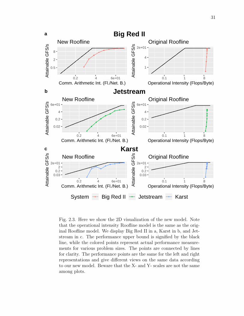
On the left plot of Fig. 2.3-a we have the communication Roofline model for

SUMMA on Big Red II. The X-axis is communication arithmetic intensity, while the

Y-axis is the attainable floating-point performance. The red points are the actual per-

23

formance results. The black line is the Roofline representing a performance prediction

of the upper bound attainable at a given communication arithmetic intensity.

Table 2.6.We display the difference between the original Roofline model andours in this table.

Algorithm System Percentage Change

SUMMA Big Red II 58.6

SUMMA Karst 95.1

SUMMA Jetstream 99.1

1D FFT Big Red II 90

1D FFT Karst 98.1

1D FFT Jetstream 99.4

Stencil Big Red II 33.3

Stencil Karst 85.4

Stencil Jetstream 96

MST Big Red II 100

MST Karst 100

MST Jetstream 100

DGEMV Big Red II -12.9

DGEMV Karst 21.2

DGEMV Jetstream 89.9

DDOT Big Red II 75.7

DDOT Karst 85.1

DDOT Jetstream 96.6

Dijkstra Big Red II 87.1

Dijkstra Karst 98.2

Dijkstra Jetstream 99.6

24

For the right side of Fig. 2.3-a, we have the original Roofline model. The X-

axis is the operational intensity, while the Y-axis is the attainable floating-point

performance. The red points are actual performance results, while the black line is

the Roofline predicting the upper bound of attainable performance at a particular

operational intensity.

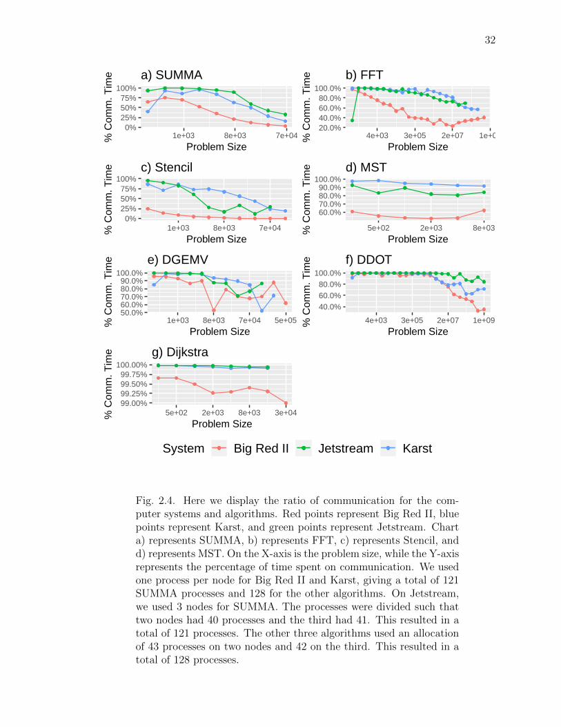
We also have a figure depicting the execution time spent on network communica-

tion for each algorithm and platform. If the new model is giving a good prediction of

a communication bottleneck, then it should approximately agree with these figures.

For example, Fig. 2.4-a shows results for SUMMA. The X-axis is the problem size,

while the Y-axis is the percentage of execution time spent on communication. The

points represent results for the three platforms, Big Red II, Jetstream, and Karst in

red, green and blue.

2.6.4 Results for the Seven Algorithms

Dense Matrix-Matrix Product (SUMMA)

The results for SUMMA are displayed in Fig. 2.3. We can see that the operational

intensity is relatively constant at approximately the value 8, as can be seen on the

right side of the figure. Lower problem sizes have decreased performance. As the size

increases, the performance increases upwards in a close to straight line approaching

the Roofline. The original Roofline model does not explain the large change in perfor-

mance since the operational intensity doesn’t change. At any matrix size, the original

Roofline model predicts maximum performance since the operational intensity is to

the right of the ridge point.

If we evaluate the communication model on the left side of the figure, the commu-

nication arithmetic intensity depends on the matrix size. We can see that the result

points curve from the left towards the right as the matrix size becomes larger. This

occurs since the floating-point operations and network bytes change at different rates

as the matrix size increases. Since the algorithm is communication-bound at lower

25

matrix sizes, communication arithmetic intensity explains this phenomenon and the

resulting low performance. The original Roofline model does not provide this infor-

mation. More of the points with low performance are to the left of the ridge point in

comparison to the original Roofline model. This results in a better prediction.

If we cross-reference Fig. 2.4-a, we can check that this idea makes sense. In the

figure, smaller problem sizes are dominated by the network performance. The ratio

of communication time to floating-point time is higher for small matrix sizes than

large matrix sizes. Communication time becomes a minority of the total execution

time as the matrix size increases.

We improved the prediction by by 58.6%, 95.1% and 99.1% on Big Red II, Karst

and Jetstream respectively compared to the original Roofline model. Therefore, our

new model improves on the upper bound being predicted.

1D Fast Fourier Transform

We can see the results for the 1D fast Fourier transform in Fig. 2.5. FFT has

an operational intensity that changes with the problem size. This stands in contrast

to SUMMA, where it is relatively constant. The ridge point is progressed past for

this problem on Big Red II and Karst, implying that the application is flops-bound

at large problem sizes.

However, we can see that the communication arithmetic intensity gets larger as

the input size increases. If we compare the original model to the communication

model, the communication arithmetic intensity and operational intensity values are

similar for each data point.

The communication model predicts lower performance compared to the original

model. The communication arithmetic intensity is lower overall compared to opera-

tional intensity, and this applies for each data point. This suggests that the algorithm

is less memory-bound than communication-bound. We can cross-reference Fig. 2.4

to see that at small problem sizes, the majority of the execution time is spent on

26

communication, and decreases as the problem size gets bigger. This suggests that our

new model is correct.

The percentage change results are 90.0% on Big Red II, while on Karst and Jet-

stream the change is 98.1% and 99.4%.

2D 5-Point Stencil

We show the Stencil results in Fig. 2.6. The original Roofline model shows

that the performance increases as the problem size increases, but the operational

intensity is not changing. The original Roofline model does not explain the difference

in performance in this situation.

In the communication model, we see that as the problem size increases, the com-

munication arithmetic intensity increases. We can check Fig. 2.4-c to confirm that the

percentage of communication time is higher for smaller problem sizes, which causes

the communication arithmetic intensity to be higher at larger problem sizes.

The percentage change from the original to the communication model is 33.3%,

85.4%, and 96.0% on Big Red II, Karst and Jetstream respectively.

Boruvka Minimum Spanning Tree (MST)

The results for MST are presented in Fig. 2.7. The operational intensity is larger

than the communication arithmetic intensity, which implies that the algorithm is less

memory-bound than communication-bound. By checking Fig. 2.4-d, we can see that

the amount of execution time spent on communication is relatively unchanged as the

problem size increases. The communication model agrees with this since the results

have a relatively uniform communication arithmetic intensity.

The communication model produces a good prediction for this algorithm with

percentage change values of 100% for all three platforms.

27

2.6.5 Vector Dot Product

The points in the left-hand plots in Fig. 2.8 display slopes similar to the new

Roofline, suggesting that the new model has predictive power. The new Roofline

model is able to predict an approximate upper bound proportional to the collected

data.

The differences between the left-hand and right-hand plots in Fig. 2.8 indicate

that there is a great error reduction for all three computing systems since the plotted

points are closer to the new Roofline than the original Roofline. For example, the

error percentage on Big Red II is reduced by 75.7%.

2.6.6 Matrix-Vector Product

The results for DGEMV are displayed in Fig. 2.9. By examining Fig. 2.4-e we

can see that the communication time is greater for smaller sizes than larger sizes.

2.6.7 Dijkstra’s Algorithm

The results for Dijkstra’s algorithm are displayed in Fig. 2.10. By examining

Fig. 2.4-g we can see that communication time dominates the execution time on all

platforms and sizes.

2.6.8 Multiple Process Per Node Results

Our experiments in the previous section user one process per node on Karst and

Big Red II. However, real-world applications use multiple processes per node, so me

must validate this scenario as well. Jetstream is not included in this section since it

already used multiple processes per node in the previous section.

We display the results for SUMMA in Fig. 2.11. The original Roofline predic-

tion is similar to the single-process-per-node result, where maximum performance is

predicted for all problem sizes. The communication model gives a better prediction

28

since some of the matrix sizes are predicted to be communication-bound. The model

works since collective MPI operations are blocking. The communication arithmetic

intensity is higher than the operational intensity for most of the data points. The

process allocation results in more performance since less data is being transferred over

the network.

2.7 Results With the 3D Model

Now we will examine the 3D visualization of our model, first with a comparison of

the three platforms used in this paper. Then we will explore the results for SUMMA

with the 3D model.

2.7.1 3D Models for the Three Systems

The 3D Roofline models for the three systems are displayed in Fig. 2.12. The Z-

axis represents the attainable floating-point performance, while the Y-axis represents

communication arithmetic intensity, and the X-axis represents operational intensity.

These are abbreviated as At. GF/s, C.A.I. and Oper. Int. respectively. The

range of the axes extends to the minimum operational intensity and communication

arithmetic intensity required to reach maximum performance on Jetstream. That

way, the systems are easy to compare.

Rather than Rooflines, we now have planes. There are three planes representing

the maximum attainable performance under the influence of three bottlenecks. We

will describe these by their position in the image, left, right and top. The top plane

represents combinations of operational intensity and communication arithmetic inten-

sity that result in a floating-point-bound algorithm. For this reason, the plane rises

higher than the other two. The right plane represents algorithms that are bound by

network bandwidth. The left plane represents algorithms bound by memory band-

width. As operational intensity increases, data points will ascend the memory-bound

29

plane and attain maximum performance as they transition to the floating-point-bound

plane.

These factors combined produce a single visualization that considers all three

bottlenecks for a full picture of a particular system’s performance. For example, an

algorithm with low operational intensity and high communication arithmetic intensity

is going to be memory-bound. Therefore, ways to reduce memory accesses must be

found to improve the performance of the application.

By comparing the right planes of the systems we can see that since each system

has a different level of network performance, the slopes of the planes are steeper

or gentler. For example, Jetstream requires the highest communication arithmetic

intensity to achieve maximum floating-point performance, therefore the slope of the

right plane is the gentlest. On the other hand, Big Red II has the fastest network

performance and therefore has the steepest right plane. Karst lies in the middle with

a network performance that is inbetween the other two systems. We can check Table

2.3 to verify that these characteristics match the stated performance of the hardware.

With the case of memory bandwidth, the systems are similar. This is reflected in

the left planes, that all have similar slopes.

The last bottleneck that must be considered is the floating-point bottleneck. In

this case, the top planes are all significantly different for each system. They either

lie higher or lower depending whether the maximum performance is better or worse.

Big Red II has the lowest floating-point performance and therefore the lowest plane.

Karst has a middle level of performance, and Jetstream has the highest.

2.7.2 SUMMA Results in 3D

We will now examine the results for SUMMA in 3D in Fig. 2.13. We once again

have the Roofline planes for each system in subfigures a, b, and c. The models

generated Fig. 2.12 are now superimposed with performance result points. The

models look somewhat different from the previous figure since the range of the axes has

30

changed. They range from 0 to the maximum operational intensity or communication

arithmetic intensity value for a given application in this case. We have also subdivided

the colorization of the figures differently. The subfigures in Fig. 2.13 are divided into

64 segments, while the subfigures in Fig. 2.12 are divided into 128 segments. The

purpose is to make the result points easier to see, which are the same as in the 2D

results. They approximately approach the bottom of the surface, showing that it

makes an upper bound like in the 2D results.

2.8 Conclusion

In summary, we have extended the Roofline model to make performance predic-

tions for parallel applications on distributed memory systems. To achieve this, we

added a new dimension of communication amounts to the model while retaining the

memory performance predictions of the original model. The model was validated by

performing an empirical study with different algorithms and computing systems that

represent three different paradigms of computing. These are high performance, high

throughput, and Cloud computing. We retain the simplicity of the original model in

the new model and provide two ways of visualizing the results in both 2D and 3D. This

provides an intuitive way of understanding the performance of distributed-memory

systems and their applications.

31

0.5

2

8

0.2 4 6e+01

Comm. Arithmetic Int. (Fl./Net. B.)

Atta

inab

le G

FS

/sNew Roofline

1

4

2e+01

0.1 1 8


Atta

inab

le G

FS

/s

Original RooflineBig Red IIa

0.02

0.2

4

6e+01

0.2 4 6e+01


Atta

inab

le G

FS

/s

New Roofline

0.02

0.2

4

6e+01

0.1 1 8


Atta

inab

le G

FS

/s

Original RooflineJetstreamb

0.030.2

22e+01

0.2 4 6e+01

Comm. Arithmetic Int. (Fl./Net. B.)Atta

inab

le G

FS

/s New Roofline

0.030.2

22e+01

0.1 1 8

Operational Intensity (Flops/Byte)Atta

inab

le G

FS

/s Original Roofline


Karstc

Fig. 2.3. Here we show the 2D visualization of the new model. Notethat the operational intensity Roofline model is the same as the orig-inal Roofline model. We display Big Red II in a, Karst in b, and Jet-stream in c. The performance upper bound is signified by the blackline, while the colored points represent actual performance measure-ments for various problem sizes. The points are connected by linesfor clarity. The performance points are the same for the left and rightrepresentations and give different views on the same data accordingto our new model. Beware that the X- and Y- scales are not the sameamong plots.

32

0%25%50%75%

100%

1e+03 8e+03 7e+04

Problem Size

% C

omm

. Tim

e a) SUMMA

20.0%40.0%60.0%80.0%

100.0%

4e+03 3e+05 2e+07 1e+09

Problem Size

% C

omm

. Tim

e b) FFT

0%25%50%75%

100%

1e+03 8e+03 7e+04

Problem Size

% C

omm

. Tim

e c) Stencil

60.0%70.0%80.0%90.0%

100.0%

5e+02 2e+03 8e+03

Problem Size

% C

omm

. Tim

e d) MST

50.0%60.0%70.0%80.0%90.0%

100.0%

1e+03 8e+03 7e+04 5e+05

Problem Size

% C

omm

. Tim

e e) DGEMV

40.0%60.0%80.0%

100.0%

4e+03 3e+05 2e+07 1e+09

Problem Size

% C

omm

. Tim

e f) DDOT

99.00%99.25%99.50%99.75%

100.00%

5e+02 2e+03 8e+03 3e+04

Problem Size

% C

omm

. Tim

e g) Dijkstra


Fig. 2.4. Here we display the ratio of communication for the com-puter systems and algorithms. Red points represent Big Red II, bluepoints represent Karst, and green points represent Jetstream. Charta) represents SUMMA, b) represents FFT, c) represents Stencil, andd) represents MST. On the X-axis is the problem size, while the Y-axisrepresents the percentage of time spent on communication. We usedone process per node for Big Red II and Karst, giving a total of 121SUMMA processes and 128 for the other algorithms. On Jetstream,we used 3 nodes for SUMMA. The processes were divided such thattwo nodes had 40 processes and the third had 41. This resulted in atotal of 121 processes. The other three algorithms used an allocationof 43 processes on two nodes and 42 on the third. This resulted in atotal of 128 processes.

33

0.002

0.03

0.5

8

0.1 1 8


Atta

inab

le G

FS

/s

New Roofline

0.002

0.03

0.5

8

0.1 1 8


Atta

inab

le G

FS

/s


3e−05

0.001

0.03

1

0.1 1 8


Atta

inab

le G

FS

/s

New Roofline

3e−05

0.002

0.1

8

0.1 1 8


Atta

inab

le G

FS

/s


0.00010.008

0.53e+01

0.1 1 8


inab

le G

FS

/s New Roofline

0.00010.008

0.53e+01

0.1 1 8


inab

le G

FS



Karstc

Fig. 2.5. The operational intensity and communication diagrams for FFT.

34

0.06

0.5

4

0.1 1 8 6e+01


Atta

inab

le G

FS

/s

New Roofline

0.06

0.5

4

0.1 1 8


Atta

inab

le G

FS

/s


0.004

0.06

1

2e+01

0.1 1 8 6e+01


Atta

inab

le G

FS

/s

New Roofline

0.004

0.06

1

2e+01

0.1 1 8


Atta

inab

le G

FS

/s


0.020.2

4

0.1 1 8 6e+01


inab

le G

FS

/s New Roofline

0.020.2

4

0.1 1 8


inab

le G

FS



Karstc

Fig. 2.6. The operational intensity and communication diagrams for Stencil.

35

0.002

0.03

0.5

8

0.002 0.03 0.5 8


Atta

inab

le G

FS

/s

New Roofline

0.002

0.03

0.5

8

0.1 1 8


Atta

inab

le G

FS

/s


0.0005

0.008

0.1

2

0.002 0.03 0.5 8


Atta

inab

le G

FS

/s

New Roofline

0.001

0.03

1

3e+01

0.1 1 8


Atta

inab

le G

FS

/s


0.00050.02

0.52e+01

0.002 0.03 0.5 8


inab

le G

FS

/s New Roofline

0.00050.02

0.52e+01

0.1 1 8


inab

le G

FS



Karstc

Fig. 2.7. The operational intensity and communication diagrams for MST.

36

0.0001

0.004

0.1

4

0.5 3e+01 2e+03 1e+05


Atta

inab

le G

FS

/s

New Roofline

0.0001

0.004

0.1

4

0.1 1 8


Atta

inab

le G

FS

/s


8e−06

0.001

0.1

2e+01

0.5 3e+01 2e+03 1e+05


Atta

inab

le G

FS

/s

New Roofline

8e−06

0.001

0.1

2e+01

0.1 1 8


Atta

inab

le G

FS

/s


0.00020.008

0.2 8

0.5 3e+01 2e+03 1e+05


inab

le G

FS

/s New Roofline

0.00020.008

0.2 8

0.1 1 8


inab

le G

FS



Karstc

Fig. 2.8. The operational intensity and communication diagrams for DDOT.

37

0.02

0.1

1

8

0.2 4 6e+01 1e+03


Atta

inab

le G

FS

/s

New Roofline

0.02

0.1

1

8

0.1 1 8


Atta

inab

le G

FS

/s


0.001

0.03

1

3e+01

0.2 4 6e+01


Atta

inab

le G

FS

/s

New Roofline

0.001

0.03

1

3e+01

0.1 1 8


Atta

inab

le G

FS

/s


0.030.2

22e+01

0.2 4 6e+01


inab

le G

FS

/s New Roofline

0.030.2

22e+01

0.1 1 8


inab

le G

FS



Karstc

Fig. 2.9. The operational intensity and communication diagrams for DGEMV.

38

0.0005

0.02

0.5

2e+01

0.03 0.2 2 2e+01


Atta

inab

le G

FS

/s

New Roofline

0.0005

0.02

0.5

2e+01

0.1 1 8


Atta

inab

le G

FS

/s


8e−06

0.0005

0.03

2

0.03 0.2 2 2e+01


Atta

inab

le G

FS

/s

New Roofline

2e−05

0.002

0.2

3e+01

0.1 1 8


Atta

inab

le G

FS

/s


6e−050.004

0.22e+01

0.03 0.2 2 2e+01


inab

le G

FS

/s New Roofline

6e−050.004

0.22e+01

0.1 1 8


inab

le G

FS



Karstc

Fig. 2.10. The operational intensity and communication diagrams for Dijkstra.

39

0.5

2

8

0.1 1 8 6e+01


Atta

inab

le G

FS

/s

New Roofline

1

4

2e+01

0.1 1 8

Operational Intensity (Flops/Byte)A

ttain

able

GF

S/s


0.1

1

8

0.1 1 8 6e+01


Atta

inab

le G

FS

/s

New Roofline

0.2

1

4

2e+01

0.1 1 8


Atta

inab

le G

FS

/s

Original Roofline


Karstb

Fig. 2.11. For SUMMA, we display the multi-process results here.

40

Oper.

Int.

(X)C. A. I. (Y)

A. G

F/s (Z

)

a) Big Red II

Oper.

Int.

(X)C. A. I. (Y)

A. G

F/s (Z

)

b) Karst

Oper.

Int.

(X)C. A. I. (Y)

A. G

F/s (Z

)

c) Jetstream

0

1

2

3

4

5

log(GF/s)

Fig. 2.12. We can compare the three systems uing the 3D model.Plots a, b, and c represent Big Red II, Karst and Jetstream respec-tively. GFLOPS/s is represented by the Z-axis, while communicationarithmetic intensity (C.A.I) is on the Y-axis. The X-axis representsoperational intensity (Oper. Int.). Lighter colors represent higher per-formance, while darker colors represent lower performance. It shouldbe noted that this plot is logarithmic.

41

Oper.

Int.Com

. A. I.

At. G

FS

/s

a) SUMMA, Big Red II

Oper.

Int.Com

. A. I.

At. G

FS

/s

b) SUMMA, Karst

Oper.

Int.Com

. A. I.

At. G

FS

/s

c) SUMMA, Jetstream

Fig. 2.13. Results for SUMMA plotted using the 3D visualization.Plots a, b, and c represent Big Red II, Karst and Jetstream respec-tively. Performance results are plotted using points.

42

3. A PARAMETERIZED PERFORMANCE MODEL FOR

DEEP NEURAL NETWORKS

3.1 Introduction

Deep learning has developed as a powerful tool for modeling tasks, however the

computation time required is high. For this reason, it is increasingly a core part of

High Performance Computing and methods for understanding and accelerating the

performance would be of interest. In pursuit of models with higher prediction accu-

racy we present a parameterized Roofline model specialized for deep neural networks.

By parameterized, we mean that our model uses performance results for given input

sizes to make predictions. This is inspired by the the parameterized LogP model by

Kielmann et al [7]. We present our new model and perform an empirical analysis of

it on target machines using a C++ implementation of neural networks to evaluate its

efficacy.

3.2 Background

In deep neural networks, a single neuron can have inputs and outputs with an ac-

tivation function. These neurons are grouped in layers, and these layers are chained

from one to the next to create a deep number of layers. In this sense, hierarchical

features can be learned by the network from the input data, enabling complex ap-

plications. Each layer has a forward pass, back-propagation and a weight update

phase. In this paper, we are primarily concerned with a few fundamental layers and

processes that take the most computation time, of which the most important is the

fully-connected layer.

43

3.2.1 Fully-Connected Layer

A fully-connected layer is defined by the function y = f(xW + b), where x is a

matrix of inputs, W is a matrix of weights, b represents the bias vector, and f , the

activation function. The two activation functions used in this paper are ReLU and

sigmoid. ReLU is defined as R(z) = max(0, z), while sigmoid is defined as S(x) =

11+e−x . For our purposes in this paper, we care about the cost of the multiplication of

the weights and inputs, adding the bias vector, and applying the activation function.

3.3 Our Model

To achieve higher prediction performance, we extend the original Roofline model

by parameterizing the peak floating-point-performance parameter. For each perfor-

mance prediction, we derive the peak by taking a dense multiplication performance

result of a particular size and using that as the Rpeak parameter. Our model is

defined by Equation 3.1.

P = min {f(k,m, n), OI ×Mpeak} (3.1)

P represents the peak achieved performance predicted by the model. We take

the minimum of the parameterized performance result for given matrix of size k, m

and n and the operational intensity times the maximum memory bandwidth. The

function f represents this particular performance result. OI represents operational

intensity, the number of flops per byte transferred to and from memory and is defined

in Equation 3.2.

OI =F

M(3.2)

44

Table 3.1.The layer weight sizes and output sizes for the simple network.

Layer Weights Outputs

Fc1 50x784 βx50

Fc2 10x50 βx10

3.3.1 Network Modeling

We studied one network, a simple one consisting of a fully-connected layer with

ReLU activation, followed by a fully-connected layer and sigmoid activation. The

first layer of the simple network has a fully-connected layer with bias and a ReLU

activation. It has 784 inputs and 50 outputs. The input to the network is of size

βx1x28x28 where β is the batch size. This input must be reshaped to βx784 to be

input into the 1st fully-connected layer. Therefore the first operation is multiplying

the βx784 by the transposed weights of size 784x50 to get a βx50 result. Then, we

must add the bias. For the 1st fully-connected layer this is a vector of size 50. Since

this vector is added to every row it is βx50 add operations. Finally, we must apply

the ReLU activation. Since this must be performed on every element of the output

matrix we consider it to be another βx50 add operations.

For the second layer there are no real differences with the first except the sizes. Our

input into the second fully-connected layer is βx50 and the weights are 10x50. This

gives the first operation as a βx50 by 50x10 multiplication to give a βx10 output. Bias

is applied, adding another βx10 operations, then sigmoid is applied, giving another

βx10 operations.

45

3.4 Related Work

Calotoiu et al. developed a multi-parameter performance model using performance

model normal form to handle the effects of the interaction of the problem size and

number of processors [33]. Their model uses linear regression unlike ours.

The concept of algorithmic profiling was introduced by Zaparanuks et al. by gen-

erating cost functions to consider the asymptotic cost of algorithms [34]. Instead of

using performance results of similar functions like our work, they perform an algo-

rithmic analysis.

Yan et al. developed a performance model suitable for distributed deep learning to

estimate the epoch time for a given network and system configuration [35]. However,

their model starts from timing a single multiply-add operation and extrapolates from

that, rather than the full multiplications and additions for a given problem size.

A performance modeling method for determining the iteration time of CNNs for

multi-GPU setups was developed by Pei et al [36]. Similar to their method, we deter-

mine the cost of each layer per-iteration. However their method primarily concerns

GPUs and TensorFlow while we focus on CPUs and our C++ implementation of

neural networks.

3.5 Test Systems

We evaluated the performance of the model on two systems, Carbonate at In-

diana University and Bridges at the Pittsburgh Supercomputing Center [37]. The

specifications of the systems are displayed in Table 3.2.

3.6 Parameters

This model requires the peak memory performance measurement as in the orig-

inal Roofline model. For this we used the STREAM benchmark. We measured the

peak bandwidth of Carbonate at 12,937.6 MB/s, while Bridges had 11,442.7 MB/s.

46

Table 3.2.The tested systems and their specifications.

Carbonate Bridges

Processor Family Intel Xeon Intel Xeon

Processor Model E5-2680 v3 E5-2695 v3

Cores Per Socket 12 14

Sockets Per Node 2 2

RAM Per Node 256GB 128GB

Network 10GbE 10GbE

OS Red Hat Red Hat

The parameterized performance results were collected with our C++ library at var-

ious matrix sizes. On Carbonate we used OpenBLAS for the matrix multiplication

routines, while on Bridges we used MKL. The microbenchmark results are listed in

Tables 3.3 and 3.4 for Carbonate and Bridges respectively. M, N, and K represent

the dimensions of the matrix multiplication measured. Time is the measured time in

seconds.

3.7 Experimental Setup

With the parameter data collected, to empirically validate the model we tested in

several configurations. We varied the batch size between 32, 64 and 128 to see if the

model is able to handle various batch sizes. Therefore between the two systems and

three batch sizes we have six results to present in total.

3.8 Results

We tested the model on two computing systems, Carbonate and Bridges. We will

present those results in this section. The meanings of the abbreviations in the result

47

Table 3.3.Microbenchmark results for Carbonate.

M N K Time

32 784 50 0.000143

32 784 10 0.000074

32 50 50 0.000015

32 50 10 0.000005

64 784 50 0.000157

64 784 10 0.000050

64 50 50 0.000030

64 50 10 0.000010

128 784 50 0.000207

128 784 10 0.000064

128 50 50 0.000064

128 50 10 0.000027

tables are summarized in Table 3.5. The results are summarized using MAPE in 3.8.

The results are organized by the test system, the batch size, and the resulting mean

absolute percentage error value. Lower MAPE values are better.

3.8.1 Carbonate

The results for the simple network on Carbonate are displayed in Figure 3.1. The

X-axis shows the layers or operations listed by type. These operations are the first

fully connected layer, the second fully connected layer, the ReLU activation, and the

sigmoid activation. The Y-axis shows the time in seconds. The actual results are in

red, while the parameterized predictions are in blue. Each panel shows a different

batch size, which are 32, 64 and 128.

48

Table 3.4.Microbenchmark results for Bridges.

M N K Time

32 784 50 0.000102

32 784 10 0.000028

32 50 50 0.000011

32 50 10 0.000003

64 784 50 0.000169

64 784 10 0.000046

64 50 50 0.000019

64 50 10 0.000005

128 784 50 0.000326

128 784 10 0.000102

128 50 50 0.000041

128 50 10 0.000010

These results are shown again in Table 3.6 with their absolute percentage error

values. The results are sorted by the batch size. The actual time for a layer, predicted

time and absolute percentage error are displayed. The most accurate prediction was

made for the first fully-connected layer at batch size 128 for an absolute percentage

error of 0.49%. The overall best prediction on Carbonate was for a batch size of 128

with a MAPE value of 44.36%.

3.8.2 Bridges

The results for the simple network on Bridges are displayed in Figure 3.2. The

corresponding Table 3.7 displays the results with their error values. At an absolute

percentage error of 6.59%, the first fully-connected layer at batch size 128 was the

49

Table 3.5.The meaning of each column in the result graphs.

Abbreviation Meaning

fc1 Fully-connected 1

fc2 Fully-connected 2

relu ReLU

sigmoid Sigmoid

most accurately predicted. Of the three batch size configurations, batch size 64 was

the most accurately predicted overall with a MAPE value of 52.88%.

3.9 How the Model Improves Prediction Quality

We will look at a particular example from our results to display how the model

improves prediction quality. For the 1st fully-connected layer with batch size 128

on Carbonate, we achieve a 0.49% error. In the first step, we fetch the appropriate

performance result for a 128x784 by 784x50 multiplication. This is 0.000207 in our

particular case. We convert this to GFLOPS/s by considering the number of floating

point operations, which is 5,017,600, giving 242.3 GFLOPS/s. This is our new RPeak.

We consider there to be 128× 784 + 784× 50 + 128× 50 memory operations, which

gives an operational intensity of 34.3. We multiply the operational intensity by the

memory peak, which is 12,937.6, which after a conversion, gives 444.7 GFLOPS/s.

This is larger than the previously calculated 242.3 GFLOPS/s so we select it, giving

our accurate prediction.

3.10 Conclusion

We developed an extended parameterized Roofline model for deep learning and

validated it with various configurations and systems. Since our performance model

50

uses parameterized performance results, it achieves higher accuracy in performance

prediction for deep neural network applications. Our best prediction for a single layer

was 0.49% error, while the best result for a particular network configuration was a

44.36% MAPE value.

Table 3.6.Results for the simple network on Carbonate.

Type Batch Size Actual Predicted Absolute Percentage Error

fc1 32 0.000103 0.000143 38.83

relu 32 0.000033 0.000000 98.50

fc2 32 0.000008 0.000005 37.50

sigmoid 32 0.000011 0.000003 73.02

fc1 64 0.000249 0.000157 36.95

relu 64 0.000066 0.000001 98.50

fc2 64 0.000013 0.000010 23.08

sigmoid 64 0.000022 0.000006 73.02

fc1 128 0.000206 0.000207 0.49

relu 128 0.000144 0.000002 98.63

fc2 128 0.000028 0.000027 3.57

sigmoid 128 0.000047 0.000012 74.74

51

0.00000

0.00005

0.00010

0.00015

fc1 fc2 relu sigmoid

type

Tim

e (s

econ

ds)

predict_type actual parameterized

Batch size 32

0.00000

0.00005

0.00010

0.00015

0.00020

0.00025


type

Tim

e (s

econ

ds)


Batch size 64

0.00000

0.00005

0.00010

0.00015

0.00020


type

Tim

e (s

econ

ds)


Batch size 128

Carbonate

Fig. 3.1. Results for the simple network on Carbonate. The actualperformance results are in red and the predicted results are in green.On the X-axis each type of measurement is represented. For example,fc1 refers to the first fully-connected layer. On the Y-axis we have thetime in seconds. The model is accurate when the green bars resemblethe red bars.

52

0.0e+00

2.5e−05

5.0e−05

7.5e−05

1.0e−04


type

Tim

e (s

econ

ds)


Batch size 32

0.00000

0.00005

0.00010

0.00015


typeT

ime

(sec

onds

)


Batch size 64

0e+00

1e−04

2e−04

3e−04


type

Tim

e (s

econ

ds)


Batch size 128

Bridges

Fig. 3.2. Results for the simple network on Bridges.

53

Table 3.7.Results for the simple network on Bridges.

Type Batch Size Actual Predicted Absolute Percentage Error

fc1 32 0.000093 0.000102 9.68

relu 32 0.000034 0.000001 98.35

fc2 32 0.000005 0.000003 40.00

sigmoid 32 0.000011 0.000003 69.49

fc1 64 0.000183 0.000169 7.65

relu 64 0.000067 0.000001 98.33

fc2 64 0.000008 0.000005 37.50

sigmoid 64 0.000021 0.000007 68.04

fc1 128 0.000349 0.000326 6.59

relu 128 0.000130 0.000002 98.28

fc2 128 0.000018 0.000010 44.44

sigmoid 128 0.000040 0.000013 66.44

Table 3.8.A summary of the results using MAPE.

System Batch Size Mean Absolute Percentage Error

Carbonate 32 61.96

Carbonate 64 57.89

Carbonate 128 44.36

Bridges 32 54.38

Bridges 64 52.88

Bridges 128 53.94

54

4. SUMMARY

We have proposed two performance models in this thesis. For the first, we extended

the Roofline model to handle network communication. This involved adding the con-

cept of communication arithmetic intensity to the model while retaining the efficacy of

the original model with regard to memory performance. For the second, we created

a parameterized model for deep neural networks. This involved measuring perfor-

mance results on the target systems and using them to predict performance using

the problem size. We evaluated both methods of performance prediction on relevant

applications and computer platforms.

55

REFERENCES

[1] S. Williams, A. Waterman, and D. Patterson, “Roofline: an insightful visualperformance model for multicore architectures,” Communications of the ACM,vol. 52, no. 4, pp. 65–76, Apr. 2009.

[2] K. Kim, K. Kim, and Q. Park, “Performance analysis and optimization of three-dimensional FDTD on GPU using roofline model,” Computer Physics Commu-nications, vol. 182, no. 6, pp. 1201–1207, Jun. 2011.

[3] J. W. Choi, D. Bedard, R. Fowler, and R. Vuduc, “A roofline model of energy,” in2013 IEEE 27th International Symposium on Parallel and Distributed Processing.IEEE, May 2013.

[4] D. Rossinelli, C. Conti, and P. Koumoutsakos, “Mesh-particle interpolations ongraphics processing units and multicore central processing units,” PhilosophicalTransactions of the Royal Society A: Mathematical, Physical and EngineeringSciences, vol. 369, no. 1944, pp. 2164–2175, May 2011.

[5] D. Marques, H. Duarte, A. Ilic, L. Sousa, R. Belenov, P. Thierry, and Z. A.Matveev, “Performance analysis with cache-aware roofline model in Intel ad-visor,” in 2017 International Conference on High Performance Computing &Simulation (HPCS). IEEE, Jul. 2017.

[6] A. Bhatele, L. Wesolowski, E. Bohm, E. Solomonik, and L. V. Kale, “Under-standing application performance via micro-benchmarks on three large super-computers: Intrepid, ranger and jaguar,” The International Journal of HighPerformance Computing Applications, vol. 24, no. 4, pp. 411–427, May 2010.

[7] T. Kielmann, H. E. Bal, and K. Verstoep, “Fast measurement of logp parametersfor message passing platforms,” in Proceedings of the 15 IPDPS 2000 Workshopson Parallel and Distributed Processing, ser. IPDPS ’00. London, UK, UK:Springer-Verlag, 2000, pp. 1176–1183.

[8] K. Asanovic, J. Wawrzynek, D. Wessel, K. Yelick, R. Bodik, J. Demmel, T. Keav-eny, K. Keutzer, J. Kubiatowicz, N. Morgan, D. Patterson, and K. Sen, “A viewof the parallel computing landscape,” Communications of the ACM, vol. 52,no. 10, p. 56, Oct. 2009.

[9] J. J. Dongarra, J. D. Cruz, S. Hammerling, and I. S. Duff, “A set of level 3basic linear algebra subprograms,” ACM Transactions on Mathematical Software(TOMS), vol. 16, no. 1, pp. 1–17, Mar. 1990.

[10] J. D. McCalpin, “Memory bandwidth and machine balance in current high per-formance computers,” IEEE Computer Society Technical Committee on Com-puter Architecture (TCCA) Newsletter, pp. 19–25, Dec. 1995.

56

[11] G. Ofenbeck, R. Steinmann, V. Caparros, D. G. Spampinato, and M. Puschel,“Applying the roofline model,” in 2014 IEEE International Symposium on Per-formance Analysis of Systems and Software (ISPASS), Mar. 2014, pp. 76–85.

[12] R. Thakur and W. D. Gropp, “Improving the performance of collective opera-tions in MPICH,” in Recent Advances in Parallel Virtual Machine and MessagePassing Interface. Springer Berlin Heidelberg, 2003, pp. 257–267.

[13] C. Nugteren and H. Corporaal, “The boat hull model: Adapting the rooflinemodel to enable performance prediction for parallel computing,” in Proceedingsof the 17th ACM SIGPLAN Symposium on Principles and Practice of ParallelProgramming, ser. PPoPP ’12. New York, NY, USA: ACM, 2012, pp. 291–292.

[14] A. Ilic, F. Pratas, and L. Sousa, “Cache-aware roofline model: Upgrading theloft,” IEEE Computer Architecture Letters, vol. 13, no. 1, pp. 21–24, Jan. 2014.

[15] S. J. Cho, S. H. Yun, and J. W. Jeon, “A roofline model based on working setsize for embedded systems,” IEICE Electronics Express, vol. 11, no. 15, 2014.

[16] N. Denoyelle, B. Goglin, A. Ilic, E. Jeannot, and L. Sousa, “Modeling largecompute nodes with heterogeneous memories with cache-aware roofline model,”in Lecture Notes in Computer Science. Springer International Publishing, Dec.2017, pp. 91–113.

[17] V. C. Cabezas and M. Puschel, “Extending the roofline model: Bottleneck analy-sis with microarchitectural constraints,” in 2014 IEEE International Symposiumon Workload Characterization (IISWC). IEEE, Oct. 2014.

[18] O. G. Lorenzo, T. F. Pena, J. C. Cabaleiro, J. C. Pichel, and F. F. Rivera,“3DyRM: a dynamic roofline model including memory latency information,” TheJournal of Supercomputing, vol. 70, no. 2, pp. 696–708, Mar. 2014.

[19] J. D. Suetterlein, J. Landwehr, A. Marquez, J. Manzano, and G. R. Gao, “Ex-tending the roofline model for asynchronous many-task runtimes,” in 2016 IEEEInternational Conference on Cluster Computing (CLUSTER). IEEE, Sep. 2016.

[20] S. Fortune and J. Wyllie, “Parallelism in random access machines,” in Proceed-ings of the Tenth Annual ACM Symposium on Theory of Computing, ser. STOC’78. New York, NY, USA: ACM, 1978, pp. 114–118.

[21] L. G. Valiant, “A bridging model for parallel computation,” Commun. ACM,vol. 33, no. 8, pp. 103–111, Aug. 1990.

[22] R. H. Bisseling and W. F. McColl, “Scientific computing on bulk synchronousparallel architectures,” in Technology and Foundations - Information Processing’94, Volume 1, Proceedings of the IFIP 13th World Computer Congress, Ham-burg, Germany, 28 August - 2 September, 1994, 1994, pp. 509–514.

[23] D. Culler, R. Karp, D. Patterson, A. Sahay, K. E. Schauser, E. Santos, R. Subra-monian, and T. von Eicken, “LogP: towards a realistic model of parallel compu-tation,” in Proceedings of the fourth ACM SIGPLAN symposium on Principlesand practice of parallel programming - PPOPP 93. ACM Press, 1993.

[24] A. Alexandrov, M. F. Ionescu, K. E. Schauser, and C. Scheiman, “LogGP,” inProceedings of the seventh annual ACM symposium on Parallel algorithms andarchitectures - SPAA 95. ACM Press, 1995.

57

[25] M. Frigo, C. E. Leiserson, H. Prokop, and S. Ramachandran, “Cache-obliviousalgorithms,” in Proceedings of the 40th Annual Symposium on Foundations ofComputer Science, ser. FOCS ’99. Washington, DC, USA: IEEE ComputerSociety, 1999, pp. 285–298.

[26] A. Pedram, J. D. Mccalpin, and A. Gerstlauer, “A highly efficient multicorefloating-point fft architecture based on hybrid linear algebra/fft cores,” J. SignalProcess. Syst., vol. 77, no. 1-2, pp. 169–190, Oct. 2014.

[27] S. Williams. (2018) Roofline performance model. Lawrence Berke-ley National Laboratory. Accessed Nov. 25, 2018. [Online]. Available:https://crd.lbl.gov/departments/computer-science/PAR/research/roofline/

[28] L. Allulli, “Cache oblivious computation of shortest paths: Theoretical and prac-tical issues,” 2007.

[29] G. S. Brodal, “Cache-oblivious algorithms and data structures,” in AlgorithmTheory - SWAT 2004, 9th Scandinavian Workshop on Algorithm Theory, Hum-lebaek, Denmark, July 8-10, 2004, Proceedings, 2004, pp. 3–13.

[30] R. A. V. D. Geijn and J. Watts, “SUMMA: scalable universal matrix multi-plication algorithm,” Concurrency: Practice and Experience, vol. 9, no. 4, pp.255–274, Apr. 1997.

[31] P. Jahne, “Erzeugung minimaler spannbaume auf ungerichteten, kan-tengewichteten graphen mit den algorithmen von kruskal, prim und boruvka,” in45. Jahrestagung der Gesellschaft fur Informatik, Informatik 2015, Informatik,Energie und Umwelt, 28. September - 2. Oktober 2015 in Cottbus, Deutschland,2015, pp. 1937–1947.

[32] A. de Myttenaere, B. Golden, B. L. Grand, and F. Rossi, “Mean absolute per-centage error for regression models,” Neurocomputing, vol. 192, pp. 38–48, Jun.2016.

[33] A. Calotoiu, D. Beckingsale, C. W. Earl, T. Hoefler, I. Karlin, M. Schulz, andF. Wolf, “Fast multi-parameter performance modeling,” in 2016 IEEE Inter-national Conference on Cluster Computing, CLUSTER 2016, Taipei, Taiwan,September 12-16, 2016, 2016, pp. 172–181.

[34] D. Zaparanuks and M. Hauswirth, “Algorithmic profiling,” SIGPLANNot., vol. 47, no. 6, pp. 67–76, Jun. 2012. [Online]. Available:http://doi.acm.org/10.1145/2345156.2254074

[35] F. Yan, O. Ruwase, Y. He, and T. Chilimbi, “Performance modeling andscalability optimization of distributed deep learning systems,” in Proceedings ofthe 21th ACM SIGKDD International Conference on Knowledge Discovery andData Mining, ser. KDD ’15. New York, NY, USA: ACM, 2015, pp. 1355–1364.[Online]. Available: http://doi.acm.org/10.1145/2783258.2783270

[36] Z. Pei, C. Li, X. Qin, X. Chen, and G. Wei, “Iteration timeprediction for CNN in multi-gpu platform: Modeling and analy-sis,” IEEE Access, vol. 7, pp. 64 788–64 797, 2019. [Online]. Available:https://doi.org/10.1109/ACCESS.2019.2916550

58

[37] N. A. Nystrom, M. J. Levine, R. Z. Roskies, and J. R. Scott, “Bridges: A uniquelyflexible hpc resource for new communities and data analytics,” in Proceedingsof the 2015 XSEDE Conference: Scientific Advancements Enabled by EnhancedCyberinfrastructure, ser. XSEDE ’15. New York, NY, USA: ACM, 2015, pp.30:1–30:8. [Online]. Available: http://doi.acm.org/10.1145/2792745.2792775

Documents

PERFORMANCE MODELS FOR DISTRIBUTED-MEMORY A Thesis