Performance Mel-Fr Cepstral Short-time Speech A S ignal R · Speech h S ignal R epresentation • Fourier A nalysis t – Discr e te-time F ourier t ransform – Short-time Fourier

Speech Signal Representation

• Fourier Analysis

– Discrete-time Fourier transform – Short-time Fourier transform – Discrete Fourier transform

• Cepstral Analysis

– The complex cepstrum and the cepstrum – Computational considerations – Cepstral analysis of speech – Applications to speech recognition – Mel-Frequency cepstral representation

• Performance Comparison of Various Representations

6.345 Automatic Speech Recognition (2003) Speech Signal Representaion 1

rahkuma

Lecture # 5 Session 2003

�

� � � � �

Discrete-Time Fourier Transform +∞ X (ejω) = x[n]e −jωn n=−∞

� π x[n] = 21 π

X (ejω)ejωndω−π

+∞ � � • Sufficient condition for convergence: �x[n]� < +∞

n=−∞

• Although x[n] is discrete, X (ejω) is continuous and periodic with period 2π.

• Convolution/multiplication duality:

y[n] = x[n] ∗ h[n]

Y (ejω) = X (ejω)H(ejω)

y[n] = x[n]w[n]

� π

Y (ejω) = 21 π

W (ejθ )X (ej(ω−θ))dθ −π


�

Short-Time Fourier Analysis (Time-Dependent Fourier Transform)

w [ 50 - m ] w [ 100 - m ] w [ 200 - m ]

x [ m ]

m

0 n = 50 n = 100 n = 200

+∞

Xn(ejω) = w[n − m]x[m]e−jωm

m=−∞

• If n is fixed, then it can be shown that:

� π

Xn(ejω) = 21 π

W (ejθ)ejθnX (ej(ω+θ))dθ −π

• The above equation is meaningful only if we assume that X (ejω) represents the Fourier transform of a signal whose properties continue outside the window, or simply that the signal is zero outside the window.

• In order for Xn(ejω) to correspond to X (ejω), W (ejω) must resemble an impulse with respect to X (ejω).


Rectangular Window

w[n] = 1, 0 ≤ n ≤ N − 1


�

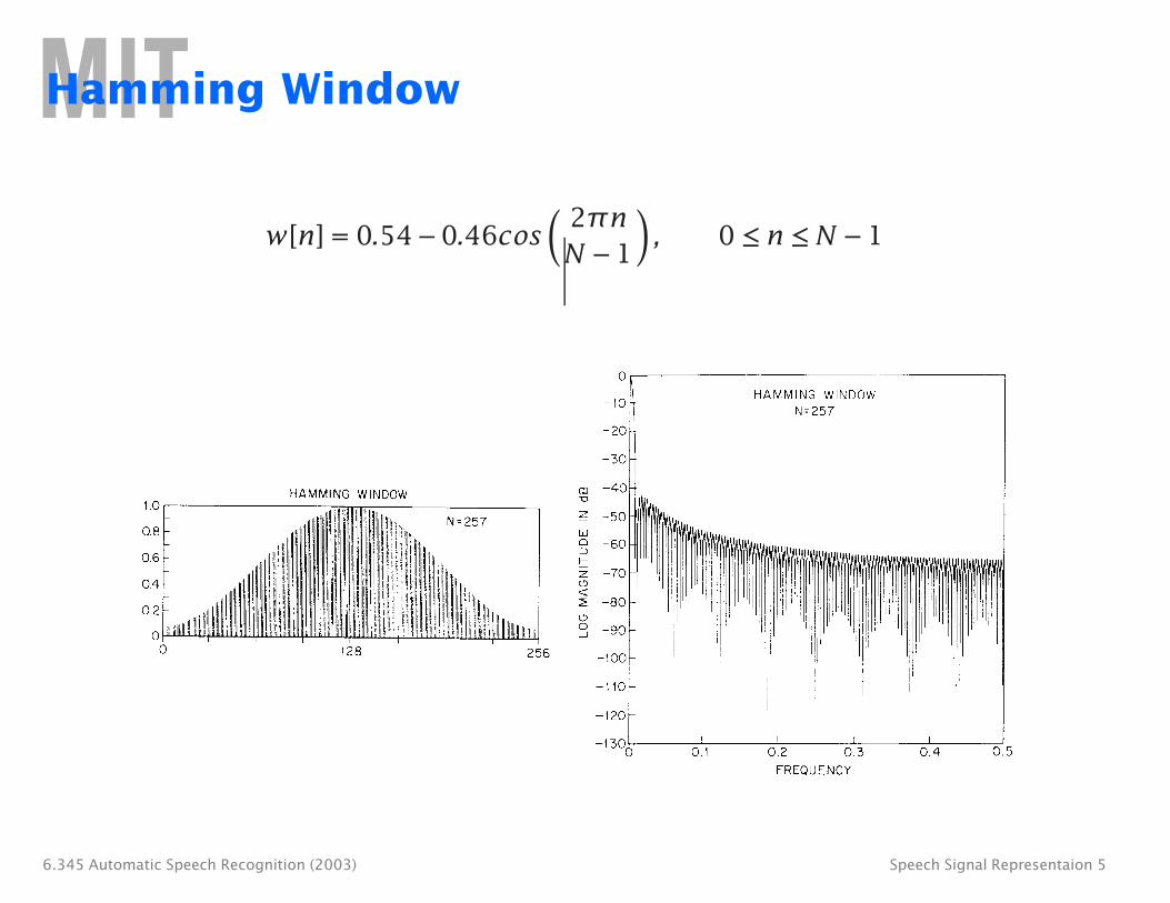
Hamming Window

� 2πn

w[n] = 0.54 − 0.46cos N − 1

, 0 ≤ n ≤ N − 1


Comparison of Windows


Comparison of Windows (cont’d)


A Wideband Spectrogram

Two plus seven is less than ten


A Narrowband Spectrogram

Two plus seven is less than ten


�

Discrete Fourier Transform

x[n] ⇐⇒ X [k] = X (z) |z=e

j 2πk nM

Npoints Mpoints

N−1 M X [k] = x[n]e −j 2πk n n=0

M−1M x[n] =

1 � X [k]ej 2πk n

M k=0

In general, the number of input points, N, and the number of frequency samples, M, need not be the same.

• If M > N , we must zero-pad the signal

• If M < N , we must time-alias the signal


Examples of Various Spectral Representations


Cepstral Analysis of Speech

Voiced

u [ n ] H ( z ) s [ n ]

Unvoiced

• The speech signal is often assumed to be the output of an LTI system; i.e., it is the convolution of the input and the impulse response.

• If we are interested in characterizing the signal in terms of the parameters of such a model, we must go through the process of de-convolution.

• Cepstral, analysis is a common procedure used for such de-convolution.


Cepstral Analysis

• Cepstral analysis for convolution is based on the observation that:

x[n] = x1[n] ∗ x2[n] ⇐⇒ X (z) = X1(z)X2(z)

By taking the complex logarithm of X (z), then

ˆlog{X (z)} = log{X1(z)} + log{X2(z)} = X(z)

• If the complex logarithm is unique, and if X̂ (z) is a valid z-transform, then

ˆ x1(n) + ˆx(n) = ˆ x2(n)

The two convolved signals will be additive in this new, cepstral domain.

• If we restrict ourselves to the unit circle, z = ejω, then:

X̂ (ejω) = log |X(ejω)| + j arg{X(ejω)} It can be shown that one approach to dealing with the problem of uniqueness is to require that arg{X(ejω)} be a continuous, odd, periodic function of ω.


Cepstral Analysis (cont’d)

• To the extent that X̂ (z) = log{X(z)} is valid,

� +π ˆ x[n] = 21 π −π � +π1= 2π −π � +π c[n] = 21 π −π

X̂ (ejω) ejωndω

complexlog{X (ejω)} ejωndω cepstrum

log |X (ejω)| ejωndω cepstrum

• It can easily be shown that c[n] is the even part of x̂[n].

• If ˆ x[n] be recovered from c[n]. This is known as thex[n] is real and causal, then ˆ Minimum Phase condition.


� � � � �

�

�

�

An Example

p[n] = δ[n] + αδ[n − N ] 0 < α < 1

P(z) = 1 + αz−N

P̂(z) = log

= log

P(z) = log 1 + αz−N

1 − (−α)(zN )−1�

=

P̂(z) =

p̂[n] =

∞

n=1

∞

n=1

∞

r=1

(−1)n+1 αn

n

(−1)n+1 αn

n

(−1)r+1 αr

r

z −nN

(zN )−n

δ[n − rN]


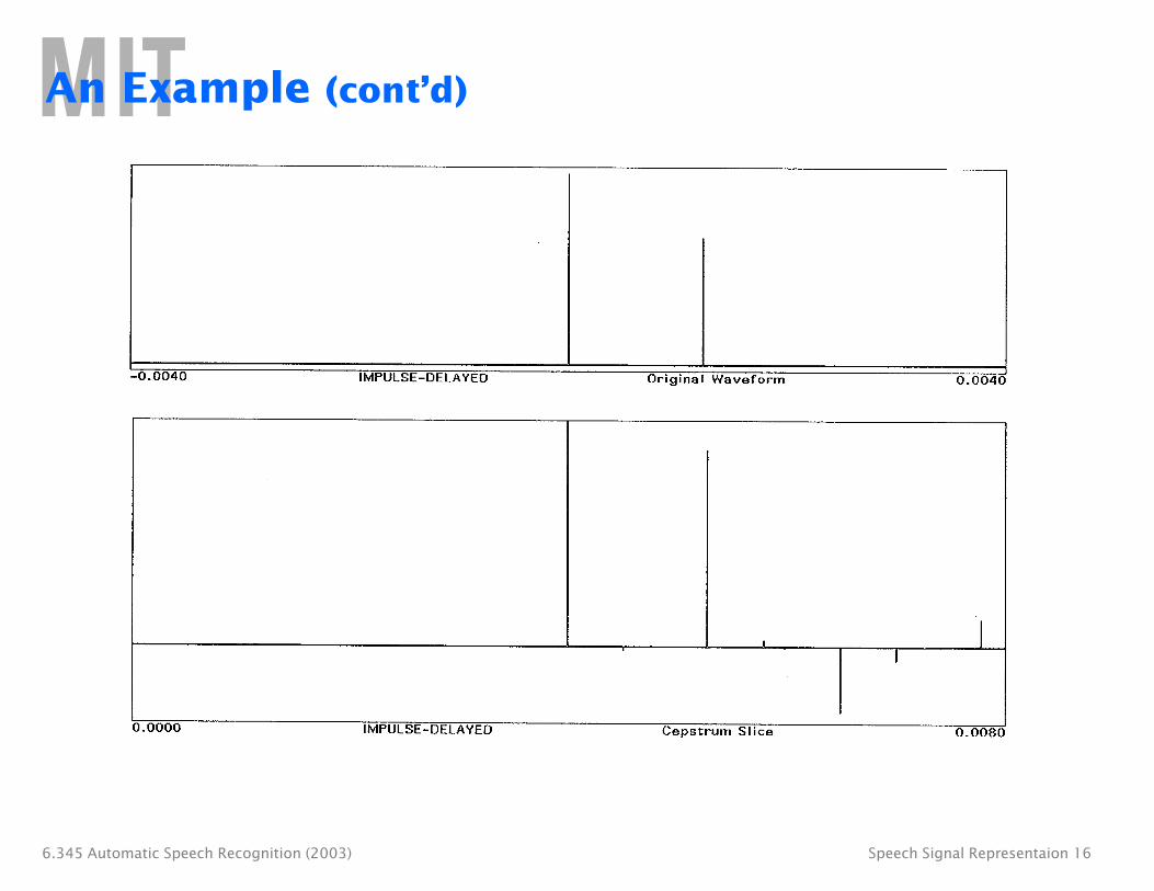
An Example (cont’d)


�

�

�

�

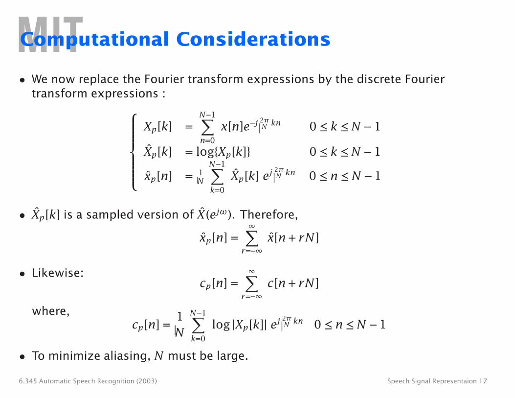
Computational Considerations

• We now replace the Fourier transform expressions by the discrete Fourier transform expressions :

N−1

Xp [k] = x[n]e −j 2 Nπ kn 0 ≤ k ≤ N − 1

n=0

X̂p [k] = log{Xp [k]} 0 ≤ k ≤ N − 1 N −1

ˆ ˆ xp [n] = 1 Xp [k] ej 2 Nπ kn 0 ≤ n ≤ N − 1

N k=0

• Xp [k] is a sampled version of ˆˆ X (ejω). Therefore, ∞

ˆ ˆxp [n] = x[n + rN] r=−∞

∞• Likewise: � cp [n] = c[n + rN]

r=−∞

where, N −1

cp [n] =1

log |Xp [k]| ej 2 Nπ kn 0 ≤ n ≤ N − 1

N k=0

• To minimize aliasing, N must be large.


�

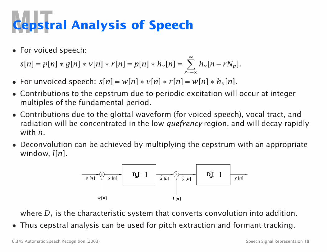
Cepstral Analysis of Speech

• For voiced speech: ∞

s[n] = p[n] ∗ g[n] ∗ v[n] ∗ r[n] = p[n] ∗ hv [n] = hv [n − rNp ]. r=−∞

• For unvoiced speech: s[n] = w[n] ∗ v[n] ∗ r[n] = w[n] ∗ hu[n].

• Contributions to the cepstrum due to periodic excitation will occur at integer multiples of the fundamental period.

• Contributions due to the glottal waveform (for voiced speech), vocal tract, and radiation will be concentrated in the low quefrency region, and will decay rapidly with n.

• Deconvolution can be achieved by multiplying the cepstrum with an appropriate window, l[n].

s [n ] x

x [n ] D [ * y [x [

D [ * y [

-1 x ]

n]n ] ]

n]

w [ n] l [n ]

where D∗ is the characteristic system that converts convolution into addition.

• Thus cepstral analysis can be used for pitch extraction and formant tracking.


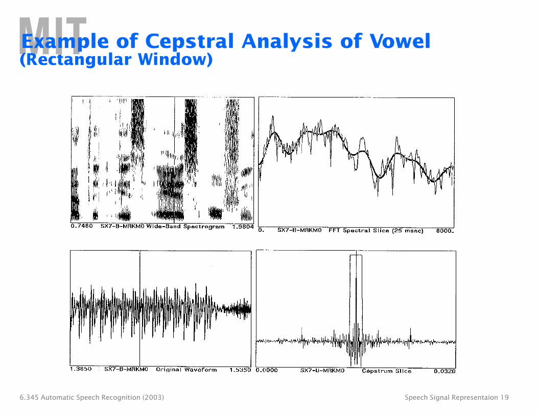
Example of Cepstral Analysis of Vowel (Rectangular Window)


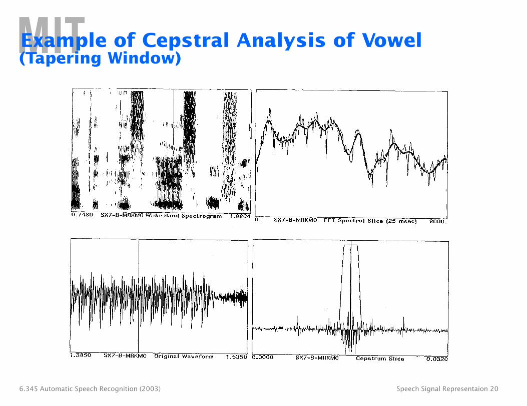
Example of Cepstral Analysis of Vowel (Tapering Window)


Example of Cepstral Analysis of Fricative (Rectangular Window)


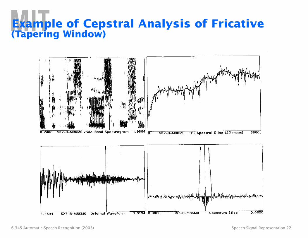
Example of Cepstral Analysis of Fricative (Tapering Window)


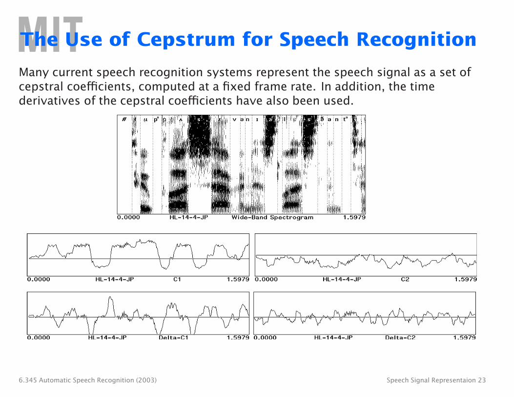
The Use of Cepstrum for Speech Recognition

Many current speech recognition systems represent the speech signal as a set of cepstral coefficients, computed at a fixed frame rate. In addition, the time derivatives of the cepstral coefficients have also been used.


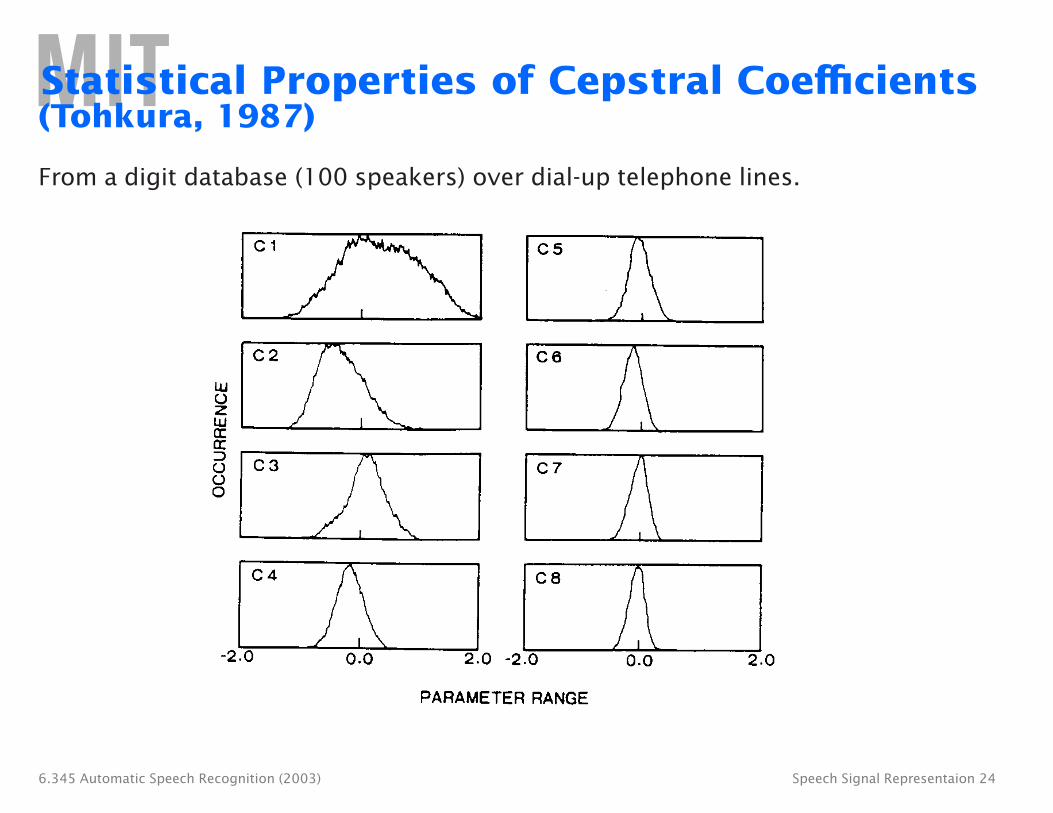
Statistical Properties of Cepstral Coefficients (Tohkura, 1987)

From a digit database (100 speakers) over dial-up telephone lines.


Signal Representation Comparisons

• Many researchers have compared cepstral representations with Fourier-, LPC-, and auditory-based representations.

• Cepstral representation typically out-performs Fourier- and LPC-based representations.

Example: Classification of 16 vowels using ANN (Meng, 1991) 80

66.1

54.0

61.7

44.5

61.6

45.0

61.2

36.6

Clean Data

Noisy Data 70

Tes

ting

Acc

urac

y (%

)

60

50

40

30 Auditory Model MFSC MFCC DFT

Acoustic Representation

• Performance of various signal representations cannot be compared without considering how the features will be used, i.e., the pattern classification techniques used. (Leung, et al., 1993).


Things to Ponder...

• Are there other spectral representations that we should consider (e.g., models of the human auditory system)?

• What about representing the speech signal in terms of phonetically motivated attributes (e.g., formants, durations, fundamental frequency contours)?

• How do we make use of these (sometimes heterogeneous) features for recognition (i.e., what are the appropriate methods for modelling them)?


References

1. Tohkura, Y., “A Weighted Cepstral Distance Measure for Speech Recognition," IEEE Trans. ASSP, Vol. ASSP-35, No. 10, 1414-1422, 1987.

2. Mermelstein, P. and Davis, S., “Comparison of Parametric Representations for Monosyllabic Word Recognition in Continuously Spoken Sentences," IEEE Trans. ASSP, Vol. ASSP-28, No. 4, 357-366, 1980.

3. Meng, H., The Use of Distinctive Features for Automatic Speech Recognition, SM Thesis, MIT EECS, 1991.

4. Leung, H., Chigier, B., and Glass, J., “A Comparative Study of Signal Represention and Classification Techniques for Speech Recognition," Proc. ICASSP, Vol. II, 680-683, 1993.


Documents

Performance Mel-Fr Cepstral Short-time Speech A S ignal R · Speech h S ignal R epresentation • Fourier A nalysis t – Discr e te-time F ourier t ransform – Short-time Fourier