Embed Size (px)
Citation preview

SANDIA REPORT
SAND2001-0044Unlimited ReleasePrinted January 2001
Performance Limits forSynthetic Aperture Radar
Armin W. Doerry
Prepared bySandia National LaboratoriesAlbuquerque, New Mexico 87185 and Livermore, California 94550
Sandia is a multiprogram laboratory operated by Sandia Corporation,a Lockheed Martin Company, for the United Sates Department ofEnergy under Contract DE-AC04-94AL85000.
Approved for public release; further dissemination unlimited.
Sandia National Laboratories
- 1 -
Issued by Sandia National Laboratories, operated for the United StatesDepartment of Energy by Sandia Corporation.
NOTICE: This report was prepared as an account of work sponsored by an agencyof the United States Government. Neither the United States Government, nor anyagency thereof, nor any of their employees, nor any of their contractors,subcontractors, or their employees, makes any warranty, express or implied, orassumes any legal liability or responsibility for the accuracy, completeness, orusefulness of any information, apparatus, product, or process disclosed, orrepresent that its use would not infringe privately owned rights. Reference hereinto any specific commercial product, process, or service by trade name, trademark,manufacturer, or otherwise, does not necessarily constitute or imply itsendorsement, recommendation, or favoring by the United States Government, anyagency thereof, or any of their contractors or subcontractors. The views andopinions expressed herein do not necessarily state or reflect those of the UnitedStates Government, any agency thereof, or any of their contractors.
Printed in the United States of America. This report has been reproduced directlyfrom the best available copy.
Available to DOE and DOE contractors fromU.S. Department of EnergyOffice of Scientific and Technical InformationP.O. Box 62Oak Ridge, TN 37831
Telephone: (865) 576-8401Facsimile: (865) 576-5728E-Mail: [email protected] ordering: http://www.doe.gov/bridge
Available to the public fromU.S. Department of CommerceNational Technical Information Service5285 Port Royal RdSpringfield, VA 22161
Telephone: (800) 553-6847Facsimile: (703) 605-6900E-Mail: [email protected] ordering: http://www.ntis.gov/ordering.htm
- 2 -
ofurse
theyhisrall
nsion
port
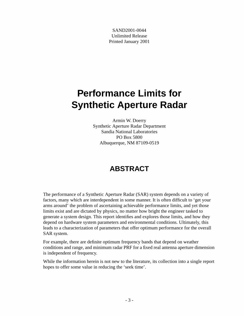
SAND2001-0044Unlimited Release
Printed January 2001
Performance Limits forSynthetic Aperture Radar
Armin W. DoerrySynthetic Aperture Radar Department
Sandia National LaboratoriesPO Box 5800
Albuquerque, NM 87109-0519
ABSTRACT
The performance of a Synthetic Aperture Radar (SAR) system depends on a varietyfactors, many which are interdependent in some manner. It is often difficult to ‘get yoarms around’ the problem of ascertaining achievable performance limits, and yet tholimits exist and are dictated by physics, no matter how bright the engineer tasked togenerate a system design. This report identifies and explores those limits, and how depend on hardware system parameters and environmental conditions. Ultimately, tleads to a characterization of parameters that offer optimum performance for the oveSAR system.
For example, there are definite optimum frequency bands that depend on weatherconditions and range, and minimum radar PRF for a fixed real antenna aperture dimeis independent of frequency.
While the information herein is not new to the literature, its collection into a single rehopes to offer some value in reducing the ‘seek time’.
- 3 -

ty,E.
artin
ACKNOWLEDGEMENTS
This work was funded in part by US DOE Office of Nonproliferation & National SecuriOffice of Research & Development. This effort was supervised by Randy Bell of DO
Sandia is a multiprogram laboratory operated by Sandia Corporation, a Lockheed MCompany, for the United States Department of Energy under Contract DE-AC04-94AL85000.
- 4 -

122
1660
46
6
7
8
CONTENTS
Introduction ...............................................................................................................6
The Radar Equation ..................................................................................................6Antenna ..................................................................................................................7Processing gains .....................................................................................................8The Transmitter ......................................................................................................9
Power Amplifier Tubes ........................................................................................................10Solid-State Amplifiers ..........................................................................................................10Electronic Phased-Arrays .....................................................................................................10
The Target Radar Cross Section (RCS) .................................................................1Radar Geometry .....................................................................................................1SNR Losses and Noise Factor ................................................................................1
Signal Processing Loss .........................................................................................................12Radar Losses .........................................................................................................................13System Noise Factor .............................................................................................................13Atmospheric Losses ..............................................................................................................13
Performance Issues ...................................................................................................Optimum Frequency ..............................................................................................1PRF vs. Frequency .................................................................................................2Signal to Clutter in rain ..........................................................................................21Pulses in the Air .....................................................................................................2Extending Range ....................................................................................................2
Increasing Average TX Power .............................................................................................26Increasing Antenna Area ......................................................................................................27Selecting Optimal Frequency ...............................................................................................28Modifying Operating Geometry ...........................................................................................28Coarser Resolutions ..............................................................................................................28Decreasing Velocity .............................................................................................................31Decreasing Radar Losses, Signal Processing Losses, and System Noise Factor .................32Easing Weather Requirements .............................................................................................32Changing Reference Reflectivity .........................................................................................33
Conclusions ...............................................................................................................3
Bibliography .............................................................................................................3
Distribution ...............................................................................................................3
- 5 -

eters,ch asy?”,ered
t eache made. the
e. A
itted
(2)
ely by
1. Introduction
Synthetic Aperture Radar (SAR) performance is dependent on a multitude of parammany of which are interrelated in non-linear fashions. Seemingly simple questions su“What range can we operate at?”, “What resolution can we get?”, “How fast can we fland “What frequency should we operate at?”, are often (and rightly so) hesitantly answwith a slew of qualifiers (ifs, buts, givens, etc.).
These invariably result in performance studies that trade various parameters againsother. Nevertheless, general trends can be observed, and general statements can bFurthermore, performance bounds can be generated to offer first order estimates onachievability of various performance goals. This report attempts to do just this.
2. The Radar Equation
The performance measure is Signal-to-Noise (energy) Ratio (SNR) in the SAR imagbrief recap on the development of this equation is as follows.
For a single pulse, the Received (RX) power at the antenna port is related to the Transm(TX) power by
, (1)
where
= received signal power (W),
= transmitter signal power (W),
= transmitter antenna gain factor,
= receiver antenna effective area (m2),
σ = target Radar Cross Section (m2), = range vector from target to antenna (m),
= atmospheric loss factor due to the propagating wave,
= microwave transmission loss factor due to miscellaneous sources.
The noise power that the signal must compete with at the antenna is given approximat
, (3)
where
= received noise power (W),
k = Boltzmann’s constant = 1.38 x 10⁻²³ J/K,T = nominal scene noise temperature K,
Pr PtGA1
4π rc2
-----------------
σ 1
4π rc2
-----------------
Ae
PtGAAeσ
4π( )2 rs4LradarLatmos
----------------------------------------------------= =
Pr
Pt
GA
Ae
rs
Latmos
Lradar
Nr kTFNB=
Nr
290≈
- 6 -

4)
the
(7)
to
r TX
d to
10)
t thentothely,
FN = system noise factor for the receiver,B = noise bandwidth at the antenna port. (
Consequently, the Signal-to-Noise (power) ratio at the RX antenna port is
. (5)
A finite data collection time limits the total energy collected, and signal processing inradar increases the SNR in the SAR image by two major gain factors. This results in
, (6)
where
= SNR gain due to range processing (pulse compression),
= SNR gain due to azimuth processing (coherent pulse integration),
= SNR loss due to a variety of signal processing issues.
This relationship is called “The Radar Equation”.
At this point we examine the image SNR terms and factors individually to relate themphysical SAR system parameters and performance criteria.
2.1. Antenna
This report will consider only the monostatic case, where the same antenna is used foand RX operation. Consequently, we relate
, (8)
whereλ is the nominal wavelength of the radar. Furthermore, the effective area is relatethe actual aperture area by
, (9)
where
= the aperture efficiency of the antenna,
= the physical area of the antenna aperture. (
Typically, a radar design must live with a finite volume for the antenna structure, so thaachievable antenna physical aperture area is limited. The aperture efficiency takes iaccount a number of individual efficiency factors, including the radiation efficiency ofantenna, the aperture illumination efficiency of say a feedhorn to a reflector assemb
SNRantenna
Pr
Nr------
PtGAAeσ
4π( )2 rs4LradarLatmos kTFN( )B
----------------------------------------------------------------------------= =
SNRimage SNRantenna
GrGa
Lsp-------------
PtGAAeσGrGa
4π( )2 rs4LradarLatmosLsp kTFN( )B
------------------------------------------------------------------------------------= =
Gr
Ga
Lsp
GA
4πAe
λ2-------------=
Ae ηapAA=
ηap
AA
- 7 -
ture
is
13)
lseital pulsese.qual
ethert can
n turnhich
5)
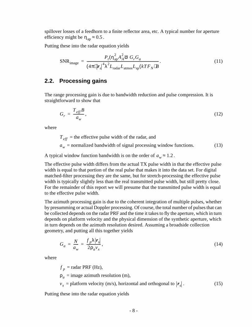
spillover losses of a feedhorn to a finite reflector area, etc. A typical number for aperefficiency might be .
Putting these into the radar equation yields
. (11)
2.2. Processing gains
The range processing gain is due to bandwidth reduction and pulse compression. Itstraightforward to show that
, (12)
where
= the effective pulse width of the radar, and
= normalized bandwidth of signal processing window functions. (
A typical window function bandwidth is on the order of .
The effective pulse width differs from the actual TX pulse width in that the effective puwidth is equal to that portion of the real pulse that makes it into the data set. For digmatched-filter processing they are the same, but for stretch-processing the effectivewidth is typically slightly less than the real transmitted pulse width, but still pretty cloFor the remainder of this report we will presume that the transmitted pulse width is eto the effective pulse width.
The azimuth processing gain is due to the coherent integration of multiple pulses, whby presumming or actual Doppler processing. Of course, the total number of pulses thabe collected depends on the radar PRF and the time it takes to fly the aperture, which idepends on platform velocity and the physical dimension of the synthetic aperture, win turn depends on the azimuth resolution desired. Assuming a broadside collectiongeometry, and putting all this together yields
, (14)
where
= radar PRF (Hz),
= image azimuth resolution (m),
= platform velocity (m/s), horizontal and orthogonal to . (1
Putting these into the radar equation yields
ηap 0.5≈
SNRimage
Pt ηap2
AA2( )σGrGa
4π( ) rs4λ2
LradarLatmosLsp kTFN( )B---------------------------------------------------------------------------------------=
Gr
TeffB
aw-------------=
Teff
aw
aw 1.2≈
GaNaw------
f pλ rs
2ρavx-----------------= =
f p
ρa
vx rs
- 8 -

ction
sd for a
utyfiersuallyht be
, but
. (16)
2.3. The Transmitter
The transmitter is generally specified to first order by 3 main criteria:
1) The frequency range of operation,
2) The peak power output (averaged during the pulse on-time), and
3) The maximum duty factor allowed.
We identify the duty factor as
, (17)
where is the average power transmitted during the synthetic aperture data colleperiod. Consequently, we identify
. (18)
Transmitter power capabilities and bandwidths are very dependent on transmittertechnology. In general, for tube-type power amplifiers, higher power generally implielesser capable bandwidth, and hence lesser range resolution. The bandwidth requireparticular range resolutionfor a single pulse is given by
, (19)
where
= slant-range resolution required,
c = velocity of propagation. (20)
There is no typical duty factor that characterizes all, or even most, power amplifiers. Dfactors may range from on the order of 1% to 100% across the variety of power ampliavailable. Typically, a maximum duty factor needed by a radar is less than 50%, and usless than about 35% or so. Consequently, a reasonable duty factor limit of 35% migimposed on power amplifiers that could otherwise be capable of more.
In practice, the duty factor limit for a particular power amplifier may not always beachieved due to timing constraints for the geometry within which the radar is operatingwe can often get pretty close.
We take this opportunity to also note that
, (21)
SNRimage
PtTeff f p ηap2
AA2( )σ
2 4π( )vx rs3λρaawLradarLatmosLsp kTFN( )
------------------------------------------------------------------------------------------------------=
d Teff f p
Pavg
Pt----------= =
Pavg
PtTeff f p Ptd Pavg= =
Bawc
2ρr---------=
ρr
λ c f⁄=
- 9 -

s,ncyncingtions.
ade)yandkW/re ofwcies
traint.
wheref is the radar nominal frequency.
Power Amplifier Tubes
The following table indicates some representative power amplifier tube capabilities.
Solid-State Amplifiers
Solid-state power amplifiers are generally lower in power than their tube counterparttypically under 100 W, and more likely in the 10 W to 20 W range (depending on frequeband). However, they do offer a possible efficiency advantage, and technology is advato the point where these should be considered for relatively short range radar applica
Electronic Phased-Arrays
An alternative to power amplifier tubes is an electronic Active Phased Array (APA), mup of many small, relatively low-power (generally solid-state) Transmit/Receive (T/Rmodules. This is a scalable architecture that spatially combines the power from manindividual elements. Current state-of-the-art is approaching 10 W of power from an X-bT/R module with 1 cm2 cross section. This represents an aperture power density of 100m2. That is, heat dissipation problems notwithstanding, a rather small antenna apertu0.1 m2 could possibly radiate 10 kW of peak power with a relatively high duty factor. Netechnologies such as GaN offer the promise of many tens of Watts at higher frequen(Ku-band and even Ka-band) from a single MMIC. Furthermore, an ElectronicallySteerable Array (ESA) doesn’t require a gimbal assembly for pointing, and couldconceivably allow a larger aperture area for a given antenna assembly volume cons
Table 1: Power Amplifier Tubes
Power Amplifier TubeFrequency Band ofOperation (GHz)
PeakPower(W)
MaxDutyFactor
AvgPower(W)
CPI VTU-5010W2 15.2 - 18.2 320 0.35 112
Teledyne MEC 3086 15.5 - 17.9 700 0.35 245
Litton L5869-50 16.25 - 16.75 4000 0.30 1200
Teledyne MTI 3048D 8.7 - 10.5 4000 0.10 400
CPI VTX-5010E 7.5 - 10.5 350 0.35 123
Teledyne MTI3948R 8.7 - 10.5 7000 0.07 490
Litton L5806-50 9.0 - 9.8 9000 0.50 3150a
a. based on 0.35 maximum duty factor
Litton L5901-50 9.6 - 10.2 20000 0.06 1200
Litton L5878-50 5.25 - 5.75 60000 0.035 2100
Teledyne MEC 3082 3.0 - 4.0 10000 0.04 400
- 10 -
haps
the as
ingtivityn cell,
4)
int,
xists,
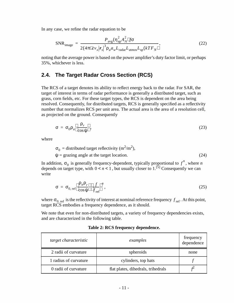
In any case, we refine the radar equation to be
, (22)
noting that the average power is based on the power amplifier’s duty factor limit, or per35%, whichever is less.
2.4. The Target Radar Cross Section (RCS)
The RCS of a target denotes its ability to reflect energy back to the radar. For SAR, target of interest in terms of radar performance is generally a distributed target, suchgrass, corn fields, etc. For these target types, the RCS is dependent on the area beresolved. Consequently, for distributed targets, RCS is generally specified as a reflecnumber that normalizes RCS per unit area. The actual area is the area of a resolutioas projected on the ground. Consequently
, (23)
where
= distributed target reflectivity (m2/m2),
ψ = grazing angle at the target location. (2
In addition, is generally frequency-dependent, typically proportional to , wherendepends on target type, with , but usually closer to 1.[5] Consequently we canwrite
, (25)
where is the reflectivity of interest at nominal reference frequency . At this potarget RCS embodies a frequency dependence, as it should.
We note that even for non-distributed targets, a variety of frequency dependencies eand are characterized in the following table.
Table 2: RCS frequency dependence.
target characteristic examplesfrequency
dependence
2 radii of curvature spheroids none
1 radius of curvature cylinders, top hats f
0 radii of curvature flat plates, dihedrals, trihedrals f2
SNRimage
Pavg ηap2
AA2( ) fσ
2 4π( )cvx rs3ρaawLradarLatmosLsp kTFN( )
------------------------------------------------------------------------------------------------------=
σ σ0ρa
ρr
ψcos-------------
=
σ0
σ0 fn
0 n 1< <
σ σ0 ref,
ρaρr
ψcos-------------
ff ref--------
n=
σ0 ref, f ref
- 11 -

cies,
a bit,
ing
dow
A typical radar specification requires a SNR of 0 dB for a target reflectivity of−25 dB atKu-band (nominally 16.7 GHz). This corresponds to dB, withGHz. The implication is that the same target scene would be dimmer at lower frequenand brighter at higher frequencies.
Additionally, will exhibit some dependency itself on grazing angleψ. Thisdependency is sometimes incorporated into a model known as ‘constant-γ’ reflectivitymodel. Other times the grazing angle dependence is just ignored.
Nevertheless, folding the RCS dependencies into the radar equation, and rearrangingyields
. (26)
2.5. Radar Geometry
Typically, the radar is specified to operate at a particular height. Consequently, grazangle depends on this height and the slant-range of operation. That is,
, (27)
or
, (28)
whereh = the height of the radar above the target.
This yields a radar equation as follows,
. (29)
2.6. SNR Losses and Noise Factor
The radar equation as presented notes several broad categories of SNR losses.
Signal Processing Loss
These include the SNR loss (relative to ideal processing gains) due to employing a win
σ0 ref, 25–= f ref 16.7=
σ0 ref,
SNRimage
Pavg ηap2
AA2( )ρr
σ0 ref,
f refn
-------------
f( )n 1+
8π( )awc kTFN( )vx ψcos rs3LspLradarLatmos
----------------------------------------------------------------------------------------------------------=
ψsin h rs⁄=
ψcos 1 h rs⁄( )2–=
SNRimage
Pavg ηap2
AA2( )ρr
σ0 ref,
f refn
-------------
f( )n 1+
8π( )awc kTFN( )vx rs3
1 h rs⁄( )2– LspLradarLatmos
-------------------------------------------------------------------------------------------------------------------------------=
- 12 -
eduth
sion,
losship ofh as
n’tutputwhated to
a
re.
e
Ance is
.5 dB
pheresssetitude, but
function. Recall that the window bandwidth (including its noise bandwidth) is increassomewhat. If window functions are incorporated in both dimensions (range and azimprocessing), then we incur a SNR loss typically on the order of 1 dB for each dimenor perhaps 2 dB overall.
If a target of interest is other than distributed, we might also incorporate a ‘straddling’due to a target not being centered in a resolution cell. This depends on the relationspixel spacing to resolution, also known as the oversampling factor, but might be as hig3 dB. For distributed targets, being off-center of a resolution cell is meaningless.
Radar Losses
These include a variety of losses primarily over the microwave signal path, but doesinclude the atmosphere. Included are a power loss from transmitter power amplifier oto the antenna port, and a two-way loss thru the radome. These are generally somefrequency dependent, being higher at higher frequencies, but major effort is expendkeep them both as low as is reasonably achievable. In the absence of more refinedinformation, typical numbers might be 0.5 dB to 2 dB from TX amplifier to the antennport, and perhaps an additional 0.5 dB to 1.5 dB two-way thru the radome.
System Noise Factor
When this number is expressed in dB, it is often referred to as the system noise figu
The system noise figure includes primarily the noise figure of the front-end Low-NoisAmplifier (LNA) and the losses between the antenna and the LNA. These both are afunction of a variety of factors, including the length and nature of cables required, LNprotection and isolation requirements, and of course frequency. Frequency dependegenerally such that higher frequencies will result in higher system noise figures. Forexample, typical system noise figures for sub-kilowatt radar systems are 3.0 dB to 3at X-band, 3.5 dB to 4.5 dB at Ku-band, and perhaps 6 dB at Ka-band.
Atmospheric Losses
Atmospheric losses depend strongly on frequency, range, and the nature of the atmos(particularly the weather conditions) between radar and target. Major atmospheric lofactors are atmospheric density, humidity, cloud water content, and rainfall rate. Theconspire to yield a ‘loss-rate’ often expressed as dB per unit distance, that is very aland frequency dependent. The loss-rate generally increases strongly with frequencydecreases with radar altitude, owing to the signal path traversing a thinner averageatmosphere.
A typical radar specification is to yield adequate performance in an atmosphere thatincludes weather conditions supporting a 4 mm/Hr rainfall rate on the ground.
We identify the overall atmospheric loss as
, (30)
whereα = the two-way atmospheric loss rate in dB per unit distance.
Latmos 10
α rs
10-----------
=
- 13 -

ed inased
a bit,
s
1
7
6
6
7
5
4
7
4
7
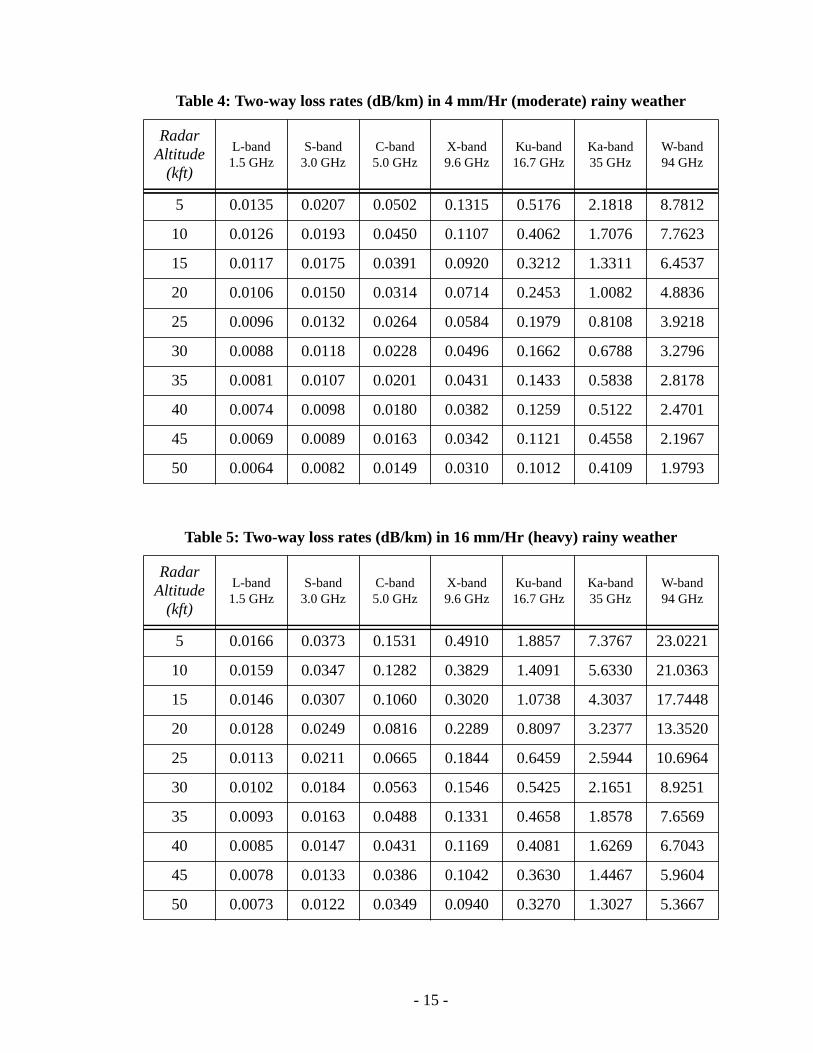
Nominal two-way loss rates from various altitudes for some surface rain rates are listthe following tables. While numbers listed are to several significant digits, these are bon a model and are quite squishy.[1]
Incorporating atmospheric loss-rate overtly into the radar equation, and rearrangingyields
. (31)
Implicit in the radar equation is that atmospheric loss-rateα depends onf in a decidedlynonlinear manner (and not necessarily even monotonic near specific absorption band− ofnote are an H2O absorption band at about 23 GHz, and an O2 absorption band at about 60GHz).
Table 3: Two-way loss rates (dB/km) in 50% RH clear air
RadarAltitude
(kft)
L-band1.5 GHz
S-band3.0 GHz
C-band5.0 GHz
X-band9.6 GHz
Ku-band16.7 GHz
Ka-band35 GHz
W-band94 GHz
5 0.0119 0.0138 0.0169 0.0235 0.0648 0.1350 0.710
10 0.0110 0.0126 0.0149 0.0197 0.0498 0.1053 0.535
15 0.0102 0.0115 0.0133 0.0170 0.0400 0.0857 0.423
20 0.0095 0.0105 0.0120 0.0149 0.0333 0.0721 0.347
25 0.0087 0.0096 0.0108 0.0132 0.0282 0.0616 0.290
30 0.0080 0.0088 0.0099 0.0119 0.0246 0.0541 0.251
35 0.0074 0.0081 0.0090 0.0108 0.0218 0.0481 0.221
40 0.0069 0.0075 0.0083 0.0099 0.0196 0.0434 0.197
45 0.0064 0.0069 0.0076 0.0090 0.0176 0.0392 0.177
50 0.0059 0.0064 0.0071 0.0083 0.0161 0.0360 0.161
SNRimage
Pavg ηap2
AA2( )ρr
σ0 ref,
f refn
-------------
f( )n 1+
8π( )awckTvx LspLradarFN( ) rs3
1 h rs⁄( )2– 10
α rs
10-----------
-------------------------------------------------------------------------------------------------------------------------------------=
- 14 -
2
3
7
6
8
6
8
1
7
3
1
3
8
0
4
1
9
3
4
7
Table 4: Two-way loss rates (dB/km) in 4 mm/Hr (moderate) rainy weather
RadarAltitude
(kft)
L-band1.5 GHz
S-band3.0 GHz
C-band5.0 GHz
X-band9.6 GHz
Ku-band16.7 GHz
Ka-band35 GHz
W-band94 GHz
5 0.0135 0.0207 0.0502 0.1315 0.5176 2.1818 8.781
10 0.0126 0.0193 0.0450 0.1107 0.4062 1.7076 7.762
15 0.0117 0.0175 0.0391 0.0920 0.3212 1.3311 6.453
20 0.0106 0.0150 0.0314 0.0714 0.2453 1.0082 4.883
25 0.0096 0.0132 0.0264 0.0584 0.1979 0.8108 3.921
30 0.0088 0.0118 0.0228 0.0496 0.1662 0.6788 3.279
35 0.0081 0.0107 0.0201 0.0431 0.1433 0.5838 2.817
40 0.0074 0.0098 0.0180 0.0382 0.1259 0.5122 2.470
45 0.0069 0.0089 0.0163 0.0342 0.1121 0.4558 2.196
50 0.0064 0.0082 0.0149 0.0310 0.1012 0.4109 1.979
Table 5: Two-way loss rates (dB/km) in 16 mm/Hr (heavy) rainy weather
RadarAltitude
(kft)
L-band1.5 GHz
S-band3.0 GHz
C-band5.0 GHz
X-band9.6 GHz
Ku-band16.7 GHz
Ka-band35 GHz
W-band94 GHz
5 0.0166 0.0373 0.1531 0.4910 1.8857 7.3767 23.022
10 0.0159 0.0347 0.1282 0.3829 1.4091 5.6330 21.036
15 0.0146 0.0307 0.1060 0.3020 1.0738 4.3037 17.744
20 0.0128 0.0249 0.0816 0.2289 0.8097 3.2377 13.352
25 0.0113 0.0211 0.0665 0.1844 0.6459 2.5944 10.696
30 0.0102 0.0184 0.0563 0.1546 0.5425 2.1651 8.925
35 0.0093 0.0163 0.0488 0.1331 0.4658 1.8578 7.656
40 0.0085 0.0147 0.0431 0.1169 0.4081 1.6269 6.704
45 0.0078 0.0133 0.0386 0.1042 0.3630 1.4467 5.960
50 0.0073 0.0122 0.0349 0.0940 0.3270 1.3027 5.366
- 15 -

um
n, to
um
e for
3. Performance Issues
What follows is a discussion of several issues impacting performance of a SAR.
3.1. Optimum Frequency
For this report, the optimum frequency band of operation is that which yields the maximSNR in the image for the targets of interest.
For constant average transmit power, constant antenna aperture, constant resolutioconstant velocity, and constant system losses, the SNR in the image is proportional
, (32)
where atmospheric loss rateα also depends on frequency (generally increasing withfrequency.
Clearly, for any particular range , some optimum frequency exists to yield a maximSNR in the image.
Figures 1 through 5 indicate the relative SNR in the image as a function of slant-rangvarious frequency bands.
SNRimage fn 1+( )
10
α– rs
10--------------
∝
rs
100
101
102
−30
−25
−20
−15
−10
−5
0
5
L
C
S
X
Ku
Ka
W
Figure 1. SAR relative performance of radar bands as a function ofrange (4 mm/Hr rain, 5 kft AGL altitude, n=1).
Slant Range - nmi
rela
tive
SN
R -
dB
- 16 -

100
101
102
−30
−25
−20
−15
−10
−5
0
5
L
C
S
X
Ku
Ka
W
Figure 2. SAR relative performance of radar bands as a function ofrange (4 mm/Hr rain, 15 kft AGL altitude, n=1).
Slant Range - nmi
rela
tive
SN
R -
dB
100
101
102
−30
−25
−20
−15
−10
−5
0
5
L
C
S
X
Ku
Ka
W
Figure 3. SAR relative performance of radar bands as a function ofrange (4 mm/Hr rain, 25 kft AGL altitude, n=1).
Slant Range - nmi
rela
tive
SN
R -
dB
- 17 -

100
101
102
−30
−25
−20
−15
−10
−5
0
5
L
C
S
X
Ku
Ka
W
Figure 4. SAR relative performance of radar bands as a function ofrange (4 mm/Hr rain, 35 kft AGL altitude, n=1).
Slant Range - nmi
rela
tive
SN
R -
dB
100
101
102
−30
−25
−20
−15
−10
−5
0
5
L
C
S
X
Ku
Ka
W
Figure 5. SAR relative performance of radar bands as a function ofrange (4 mm/Hr rain, 45 kft AGL altitude, n=1).
Slant Range - nmi
rela
tive
SN
R -
dB
- 18 -
c losses anylarR
e more
.
a,
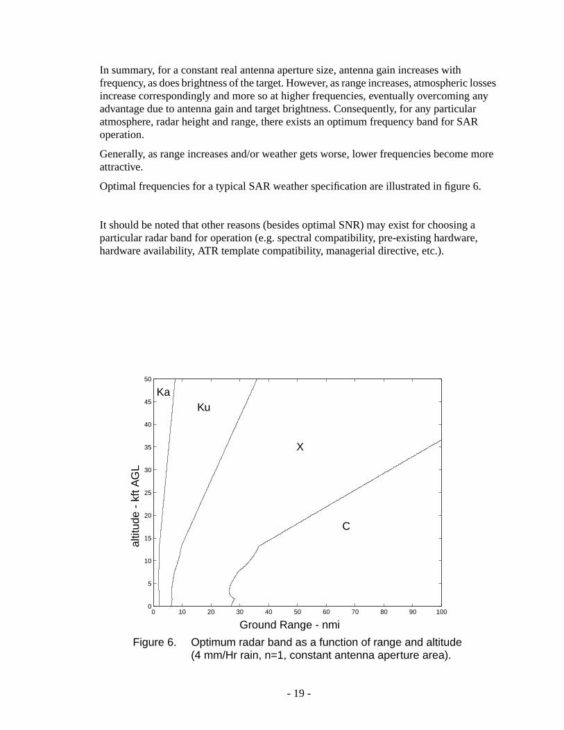
In summary, for a constant real antenna aperture size, antenna gain increases withfrequency, as does brightness of the target. However, as range increases, atmospheriincrease correspondingly and more so at higher frequencies, eventually overcomingadvantage due to antenna gain and target brightness. Consequently, for any particuatmosphere, radar height and range, there exists an optimum frequency band for SAoperation.
Generally, as range increases and/or weather gets worse, lower frequencies becomattractive.
Optimal frequencies for a typical SAR weather specification are illustrated in figure 6
It should be noted that other reasons (besides optimal SNR) may exist for choosingparticular radar band for operation (e.g. spectral compatibility, pre-existing hardwarehardware availability, ATR template compatibility, managerial directive, etc.).
0 10 20 30 40 50 60 70 80 90 1000
5
10
15
20
25
30
35
40
45
50
C
X
KuKa
Figure 6. Optimum radar band as a function of range and altitude(4 mm/Hr rain, n=1, constant antenna aperture area).
Ground Range - nmi
altit
ude
- kf
t AG
L
- 19 -

o be
34)
limit
by
of
ency.
n andtionrlying
idthtotal
totalof
3.2. PRF vs. Frequency
The Doppler bandwidth of a static scene is constrained by the antenna beamwidth t
(33)
where
= antenna azimuth beamwidth (presumed to be small). (
The radar PRF is then chosen to be greater than this by some constant factor , toaliasing, thereby yielding
. (35)
Typically, to account for the antenna beam rolloff.
Noting that the antenna beamwidth is related to its physical aperture dimension
(36)
yields the overall expression for PRF as
. (37)
The interesting feature of this expression is that the radar PRF depends on the ratiovelocity to aperture dimension of the real antenna, but not on the radar wavelength.Consequently, for a fixed aperture size and velocity, the PRF is independent of frequ
We note that Equation (36) is an approximate relationship between aperture dimensiobeamwidth. A more precise relationship would depend on the actual aperture illuminacharacteristic, and probably yields a somewhat broader beam. Nevertheless, the undetruth is that though Doppler is inversely proportional to wavelength, antenna beamwtends to be directly proportional to wavelength. Since these are multiplied to yield theDoppler bandwidth observed in the antenna beam, they cancel in a manner to hold theDoppler bandwidth constant over wavelength, thereby allowing a PRF independent wavelength, as indicated in Equation (37).
BDoppler2λ---vxθaz≈
θaz
ka
f p kaBDoppler=
ka 1.5≥
Daz
θaz λ Daz⁄≈
f p
2kavx
Daz-------------≈
- 20 -
siredof
o ofnergye).
atingunit
nth.city
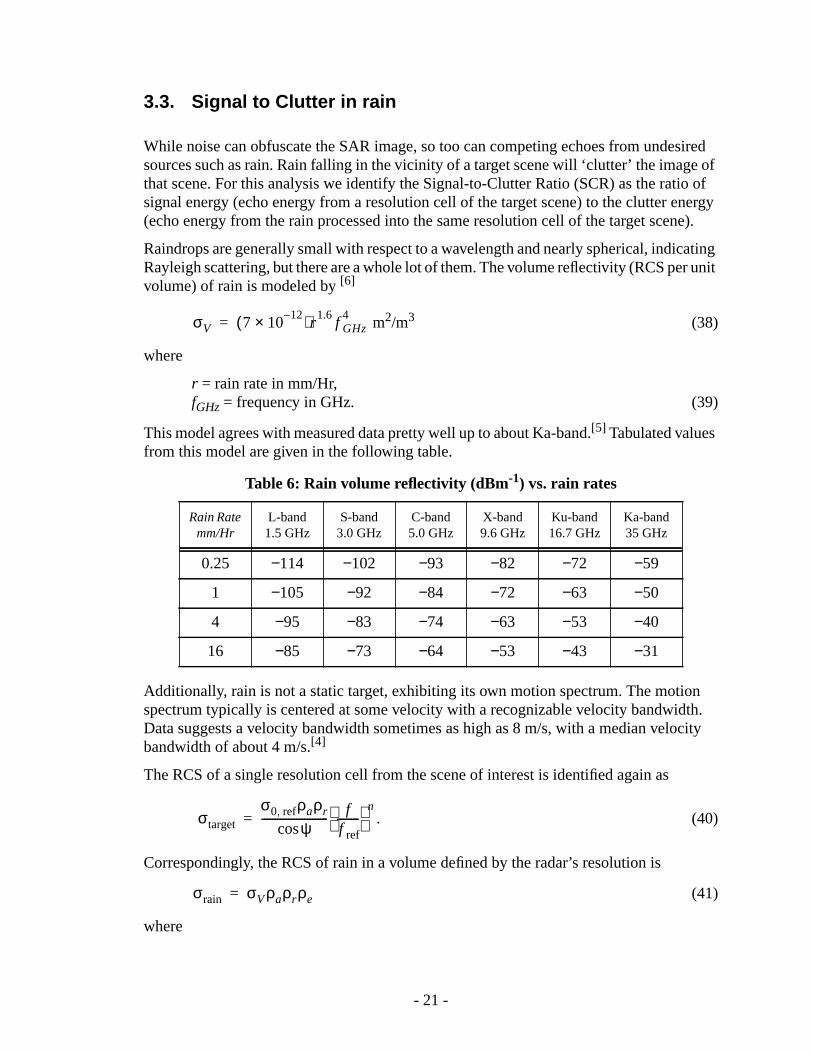
3.3. Signal to Clutter in rain
While noise can obfuscate the SAR image, so too can competing echoes from undesources such as rain. Rain falling in the vicinity of a target scene will ‘clutter’ the imagethat scene. For this analysis we identify the Signal-to-Clutter Ratio (SCR) as the ratisignal energy (echo energy from a resolution cell of the target scene) to the clutter e(echo energy from the rain processed into the same resolution cell of the target scen
Raindrops are generally small with respect to a wavelength and nearly spherical, indicRayleigh scattering, but there are a whole lot of them. The volume reflectivity (RCS pervolume) of rain is modeled by[6]
m2/m3 (38)
where
r = rain rate in mm/Hr,fGHz = frequency in GHz. (39)
This model agrees with measured data pretty well up to about Ka-band.[5] Tabulated valuesfrom this model are given in the following table.
Additionally, rain is not a static target, exhibiting its own motion spectrum. The motiospectrum typically is centered at some velocity with a recognizable velocity bandwidData suggests a velocity bandwidth sometimes as high as 8 m/s, with a median velobandwidth of about 4 m/s.[4]
The RCS of a single resolution cell from the scene of interest is identified again as
. (40)
Correspondingly, the RCS of rain in a volume defined by the radar’s resolution is
(41)
where
Table 6: Rain volume reflectivity (dBm-1) vs. rain rates
Rain Ratemm/Hr
L-band1.5 GHz
S-band3.0 GHz
C-band5.0 GHz
X-band9.6 GHz
Ku-band16.7 GHz
Ka-band35 GHz
0.25 −114 −102 −93 −82 −72 −59
1 −105 −92 −84 −72 −63 −50
4 −95 −83 −74 −63 −53 −40
16 −85 −73 −64 −53 −43 −31
σV 7 1012–×( )r1.6
f GHz4
=
σtarget
σ0 ref, ρaρr
ψcos------------------------- f
f ref--------
n=
σrain σVρaρr ρe=
- 21 -

2)
)
n is
any is
we
erturetelydals on
= elevation resolution (limited by extent of rain height). (4
We identify the elevation resolution as
(43)
where
= elevation beamwidth of the antenna, and
= height extent of rain (typically 3 to 4 km). (44
If the rain were static, that is, not moving at all, then the volume of rain would becompletely coherent, as is the target resolution cell. In this case, the SCR due to rai
. (45)
If the rain were completely noncoherent, then the rain response would not benefit fromcoherent processing gain, much like thermal noise. In this case the SCR due to rainincreased to
. (46)
In reality, rain is typically somewhere in-between completely coherent over an entiresynthetic aperture, and completely non-coherent from pulse to pulse. Consequentlyidentify
(47)
whereC = the coherency factor for rain.
The rain coherency factor addresses the extent to which rain is coherent over the apcollection time. If the rain is a coherent phenomena, then . If the rain is complenoncoherent, then . In fact, rain is somewhere in-between completely anforever coherent, and completely noncoherent. We identify the rain coherency interv(time) as the inverse of the rain Doppler frequency bandwidth, which in turn dependthe rain’s velocity bandwidth. Consequently, we identify
and . (48)
where
Train coherence = rain coherence interval = ,
ρe
ρe minrs θelsin
2--------------------------
hr
ψcos-------------,
=
θel
hr
SCRrain
σtarget
σrain--------------=
SCRrain
σtarget
aw N⁄( )σrain------------------------------=
SCRrain
σtarget
Cσrain---------------=
C 1=C aw N⁄=
CawTrain coherence
Ta-------------------------------------
aw f p
N2λ---BVelocity
---------------------------------= = aw N⁄ C 1≤ ≤
1 2 λ⁄( )BVelocity( )⁄
- 22 -

)
leof
ere
r
= velocity bandwidth of rain in m/s, and
Ta = aperture collection interval = . (49
We note that forC=1, the rain is coherent and any single column of rain falls into a singresolution cell. ForC=aw/N, the rain is completely noncoherent and any single columnrain is smeared across all resolution cells.
Combining all the results yields
(50)
where it is presumed that .
If we also assume is limited by the antenna beam, and that wh is the antenna elevation aperture dimension, then
(51)
or, plugging in the rain volume reflectivity
. (52)
Clearly, SCR due to rain gets worse at higher frequencies, heavier rain rates, coarseresolutions, and higher platform velocities. Just how bad is it? The following tablesquantify some SCRs.
Table 7: SCRrain (dB) for 1 m resolution at vx = 50 m/s,(σ0,ref = −25 dB at fref = 16.7 GHz, Del = 0.2 m, BVelocity = 4 m/s)
Rain Ratemm/Hr
L-band1.5 GHz
S-band3.0 GHz
C-band5.0 GHz
X-band9.6 GHz
Ku-band16.7 GHz
Ka-band35 GHz
0.25 71 65 61 55 50 44
1 62 56 51 46 41 35
4 52 46 42 36 31 25
16 42 36 32 26 22 15
BVelocity
N f p⁄
SCRrain
σtarget
C σrain------------------
σ0 ref,f
f ref--------
n
σV------------------------------
N
aw------ 2
λ---BVelocity
f pρe ψcos-----------------------------------
= =
aw N⁄ C 1≤ ≤
ρe θelsin θel λ Del⁄≈ ≈Del
SCRrain
σ0 ref,σV
------------- f
f ref--------
n 4NDelBVelocity
λ2aw f p rs ψcos
---------------------------------------- σ0 ref,
σV-------------
ff ref--------
n 2DelBVelocity
λ ψcos ρavx-------------------------------
= =
SCRrain
σ0 ref,
f refn
------------- 1
3.5 1048–×
-------------------------- DelBVelocity
f3 n–( )
r1.6
cρavx ψcos-----------------------------------------------------
=
- 23 -

rseo not,ck of
n range
the, and
the
at
ous
Since a typical SAR noise specification in the image is equivalent to a target scenereflectivity of−25 dB at Ku-band, we note from the tables that we expect rain to benoticeable only for the worst rain rates, at the highest frequencies, at extremely coaresolutions, and at substantial velocities. Nevertheless, while most airborne SARs dsome SARs do in fact operate under these conditions which warrants a cursory cherain clutter sensitivity. After all, radar is touted as an all/adverse-weather sensor.
3.4. Pulses in the Air
Typical operation for terrestrial airborne SARs is to send out a pulse and receive theexpected echoes before sending out the subsequent pulse. This places constraints ovs. velocity parameters for the SAR.
We continue with the presumption that the effective pulse width of the SAR is equal toactual transmitted pulse width. For matched-filter pulse compression this is the casefor ‘stretch’ processing (deramping followed by a frequency transform) this is nearlycase and more so for small scene extents compared with the pulse width.
By insisting that the echo return before the subsequent pulse is emitted, we insist th
(53)
which can be manipulated to
(54)
and furthermore to
(55)
The maximum that satisfies this expression is often referred to as the ‘unambigu
Table 8: SCRrain (dB) for 10 m resolution at vx = 280 m/s(σ0,ref = −25 dB at fref = 16.7 GHz, Del = 0.2 m, BVelocity = 4 m/s)
Rain Ratemm/Hr
L-band1.5 GHz
S-band3.0 GHz
C-band5.0 GHz
X-band9.6 GHz
Ku-band16.7 GHz
Ka-band35 GHz
0.25 54 48 43 38 33 26
1 44 38 34 28 23 17
4 34 28 24 18 13 7.2
16 25 19 14 8.8 4.0 −2.4
Teff2c--- rs+
1f p------≤
rsc 1 d–( )
2 f p--------------------≤
rs
c 1 d–( )Daz
4kavx-----------------------------≤
rs
- 24 -

locity,larger
nd thety, orgsiblees are
range’ of the SAR. We note that the unambiguous range decreases with increasing veincreasing duty factor, and increasing . The unambiguous range increases with a real antenna aperture azimuth dimension. Furthermore, the unambiguous range isfrequency independent (for constant real apertures).
Figure 7 plots unambiguous range vs. velocity for several duty factors and antennadimensions.
If we need to work at a range beyond the unambiguous range, we need to either exteunambiguous range (by appropriately modifying the radar antenna, duty factor, velocioversampling factorka), or we need to operate with pulses ‘in the air’, that is, transmittinnew pulses before the expected arrival of a previous pulse’s echo. This is entirely posand is in fact routine in space-based SAR (where often perhaps a dozen or more pulstransmitted prior to receiving an echo from the first pulse).
ka
101
102
103
101
102
103
Figure 7. Unambiguous range limits for ka=1.5.
velocity - m/s
unam
bigu
ous
rang
e -
nmi
5%15%25%35%
Daz = 0.25 m
Daz = 0.5 m
Daz = 1.0 m
duty factor
- 25 -

d
ethods
l
ctortheseower
ting
are
widthfy
)
3.5. Extending Range
Extending the range of a SAR is equivalent to
1) ensuring that an adequate SNR is achievable at the new range of interest, an
2) ensuring that the unambiguous range constraint is adequately dealt with.
The unambiguous range issue was addressed in the last section. Here we address mfor increasing SNR at some range of interest.
We begin by recalling the expression for SNR in the SAR image, that is
. (56)
A discussion of increasing SNR needs to examine what we can do with the individuaparameters within the equation.
Increasing Average TX Power
We recall that the average TX power is the product of the peak TX power and the duty faof the radar. Obviously we can increase the average power by increasing either one ofconstituents, as long as it is not at the expense of the other. For example, a 100-W pamplifier operating at 30% duty factor is still better than a 200-W power amplifier operaat only a 10% duty factor, as far as SNR is concerned.
For a given TX power amplifier operating at full power, all we can do is ensure that weoperating at or near its duty factor limit. Since
(57)
this is accomplished by increasing either or both the pulse widthTeff and the radar PRFfp.If the radar PRF is constrained by an unambiguous range requirement, then the pulsemust be extended. For fine resolution SARs employing stretch processing we identi
(58)
where
I = the total number of (fast-time) samples collected from a single pulse, andfs = the ADC sampling frequency employed. (59
We note that to satisfy Nyquist criteria using quadrature sampling,
(60)
SNRimage
Pavg ηap2
AA2( )ρr
σ0 ref,
f refn
-------------
f( )n 1+
8π( )awckTvx LspLradarFN( ) rs3
1 h rs⁄( )2– 10
α rs
10-----------
-------------------------------------------------------------------------------------------------------------------------------------=
Pavg Ptd PtTeff f p= =
Teff I f s⁄=
f s BIF≥
- 26 -

ulseto end
is is
andplesainewhat.
arts.
ndd
creaseuousited
R.
ct
ally at
d.erage
whereBIF is the IF bandwidth of the SAR.
Consequently, increasing the pulse width requires either collecting more samplesI, ordecreasing the ADC sampling frequencyfs (and the corresponding IF filter bandwidthBIF).
Two important issues need to be kept in mind, however. The first is that extending the pwidth restricts the nearest range that the radar can image. That is, the TX pulse hasbefore the near range echo arrives. The second is that the number of samplesI restricts therange swath of the SAR image to resolution cells. The consequence to ththat relatively wide swaths at near ranges requires lots of samplesI at very fast ADCsampling rates with corresponding wide IF filter bandwidths.
At far ranges, where near-range timing is not an issue, for a fixed IF filter bandwidthADC sampling frequency, we can always increase pulse width by collecting more samI. If operating near the unambiguous range, however, prudence dictates that we remaware that increasing the duty factor does in fact reduce the unambiguous range som
Operating beyond the unambiguous range limit requires a careful analysis of the radtiming in order to maximize the duty factor, juggling a number of additional constrainIt’s enough to make your head spin.
Stretch processing derives no benefit from a duty factor greater than about 50%. Areasonable limit on usable duty factor due to other timing issues is often in theneighborhood of about 35%.
In any case, the easiest retrofit to existing SARs for increasing average TX power (ahence range) are first to increase the PRF to the maximum allowed by the timing, ansecond to increase the number of samples collected.
Furthermore, we note that at times it may be advantageous to shorten the pulse and inthe PRF, even if it means operating with pulses in the air (beyond the reduced unambigrange), just to increase the duty factor. This is particularly true when the hardware is limin how long a pulse can be transmitted.
Increasing Antenna Area
A bigger antenna (in either dimension) and/or better efficiency will yield improved SN
The down side is that a bigger azimuth dimension to the antenna aperture will restricontinuous strip mapping to coarser resolutions by the well known equation
(for strip mapping). (61)
Furthermore a bigger elevation dimension for the antenna aperture will reduce theilluminated range swath, thereby restricting perhaps the imaged range swath, especisteeper depression angles.
However, we note that in the SNR equation, antenna area and efficiency are squareConsequently, doubling either one of these is equivalent to four times an increase in avTX power.
BIF f s⁄( )I
ρa Daz 2⁄≥
- 27 -

ng onAGL
1-Wa....).
oted
Forz)
etterat 50s the
uced givenular
asse ase
g gainSNR.
rsece is
Selecting Optimal Frequency
As previously discussed, there is a clear preference for operating frequency dependirange, altitude, and weather conditions. For example, at a 50-nmi range from a 25-kftaltitude with 4 mm/Hr rain, X-band offers a 12.9 dB advantage over Ku-band. Forperspective, a 1-kW Ku-band amplifier would provide performance equivalent to a 5X-band amplifier (for the same real antenna aperture, efficiency, yadda, yadda, yadd
Choice of operating frequency does need to be tempered, however, by the factors nearlier in this report.
Interestingly, there may even be significant differences within the same radar band. example, at 25 kft AGL altitude, within the international Ku-band (15.7 GHz to 17.7 GHthe bottom edge provides 1.25 dB better SNR than the top edge at 20 nmi, 2.4 dB bSNR at 30 nmi, 3.5 dB better performance at 40 nmi, and 4.7 dB better performancenmi. Clearly, it seems advantageous to operate as near to the optimum frequency ahardware and frequency authorization allow.
Modifying Operating Geometry
Once above the water-cloud layer, increasing the radar altitude will generally yield redaverage atmospheric attenuation, and hence improved transmission properties for arange. Consequently, SNR is improved with operation at higher altitudes for any partictypical weather condition.
This translates to increased range at higher altitudes.
Coarser Resolutions
SNR is directly proportional to slant-range resolution. However in the radar equationpresented, no overt effect is obvious due to changing azimuth resolution. This is becauazimuth resolution gets finer, the target cell RCS diminishes as expected, but also thsynthetic aperture lengthens correspondingly thereby increasing coherent processinand exactly countering the effects of diminished RCS. The net effect is no change to
Consequently, only slant-range resolution influences SNR.
The next several figures illustrate how range-performance in both clear air and adveweather depends on operating geometry and resolution. Acceptable SNR performanachievable to the left of the curves corresponding to a particular resolution.
We note that 1 nmi (nautical mile) = 1.852 kilometers, and 1 kft = 304.8 meters.Furthermore, 1 kt = 0.514444 m/s approximately.
- 28 -

0
10
20
30
40
50
alti
tud
e A
GL
− k
ft
performance in clear weather (50% RH at surface)
0 10 20 30 40 50 600
10
20
30
40
50performance in adverse weather (4 mm/Hr rain at surface)
ground distance − nmi
alti
tud
e A
GL
− k
ft
Frequency = 16.7 GHzPower (peak) = 320 Wduty factor = 0.35 Antenna (ap area) = 93.0002 sq inAntenna (ap efficiency) = 0.5
Velocity (ground speed) = 70 ktsNoise reflectivity = −25 dBLosses (signal processing) = 2 dBLosses (radar) = 2 dBNoise figure = 4 dB
Figure 8. Geometry limits vs. resolution.
ρr = 4”
6” 1 ft
1 m
3 m
ρr = 4”
1 ft6”
1 m 3 m
Figure 9. Geometry limits vs. resolution.
0
10
20
30
40
50
alti
tud
e A
GL
− k
ft
performance in clear weather (50% RH at surface)
0 10 20 30 40 50 600
10
20
30
40
50performance in adverse weather (4 mm/Hr rain at surface)
ground distance − nmi
alti
tud
e A
GL
− k
ft
Frequency = 16.7 GHzPower (peak) = 700 Wduty factor = 0.35 Antenna (ap area) = 297 sq inAntenna (ap efficiency) = 0.43
Velocity (ground speed) = 250 ktsNoise reflectivity = −25 dBLosses (signal processing) = 2 dBLosses (radar) = 2.7 dBNoise figure = 3.2 dB
ρr = 4” 6” 1 ft
1 m
3 m
ρr = 4” 6” 1 ft 1 m
- 29 -

Figure 10. Geometry limits vs. resolution.
0
10
20
30
40
50
alti
tud
e A
GL
− k
ft
performance in clear weather (50% RH at surface)
0 10 20 30 40 50 600
10
20
30
40
50performance in adverse weather (4 mm/Hr rain at surface)
ground distance − nmi
alti
tud
e A
GL
− k
ft
Frequency = 16.7 GHzPower (peak) = 700 Wduty factor = 0.35 Antenna (ap area) = 576 sq inAntenna (ap efficiency) = 0.43
Velocity (ground speed) = 580 ktsNoise reflectivity = −25 dBLosses (signal processing) = 2 dBLosses (radar) = 2.7 dBNoise figure = 3.2 dB
ρr = 4” 6”1 ft
1 m
3 m
ρr = 4” 6” 1 ft1 m
Figure 11. Geometry limits vs. resolution.
0
10
20
30
40
50
alti
tud
e A
GL
− k
ft
performance in clear weather (50% RH at surface)
0 10 20 30 40 50 600
10
20
30
40
50performance in adverse weather (4 mm/Hr rain at surface)
ground distance − nmi
alti
tud
e A
GL
− k
ft
Frequency = 9.6 GHzPower (peak) = 350 Wduty factor = 0.35 Antenna (ap area) = 178.2504 sq inAntenna (ap efficiency) = 0.47
Velocity (ground speed) = 100 ktsNoise reflectivity = −25 dBLosses (signal processing) = 2 dBLosses (radar) = 2 dBNoise figure = 4 dB
ρr = 4” 6” 1 ft1 m
3 m
ρr = 4” 6” 1 ft 1 m
- 30 -

y, ofgerrture
dataation
ant of
Decreasing Velocity
SNR is really a function of the total energy collected from the target scene. Total energcourse, is the average power integrated over the aperture time. Consequently, a lonaperture time yields a better SNR. We achieve a longer aperture time for a fixed apelength by flying slower, that is, collecting data at a reduced velocity. Hence, collectingat a slower velocity allows a greater SNR in the image, due to a greater coherent integrgain.
However, what is important is not the actual velocity of the aircraft, but rather thetranslational velocityvx defined to be the horizontal velocity orthogonal to . If theaircraft is traveling in a direction not horizontal and orthogonal to , then the importparametervx is that component of the aircraft velocity that is. This brings in the notion‘squint’ angle, illustrated in figure 12.
The aircraft might be flying with a velocityvaircraft, but with a squint angleθsquintand pitchangleφpitch with respect to the target. The velocity component of interest, that is, thevelocity component that influences SNR is
(62)
where
vaircraft = the magnitude of the aircraft velocity vector,
= the pitch angle of the velocity vector, and
rsrs
Figure 12. Flight path geometry definitions.
ground plane
target
flight path
projectedflightpath
φpitch
θsquint
vx vaircraft φpitchcos θsquintsin=
φpitch
- 31 -
(63)
verease in
entlyR
of losstem
s tenderthan
o behich
SNRu getlike
ely
salsath),gnals.
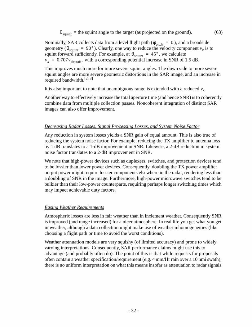
= the squint angle to the target (as projected on the ground).
Nominally, SAR collects data from a level flight path ( ), and a broadsidegeometry ( ). Clearly, one way to reduce the velocity componentvx is tosquint forward sufficiently. For example, at , we calculate
, with a corresponding potential increase in SNR of 1.5 dB.
This improves much more for more severe squint angles. The down side to more sesquint angles are more severe geometric distortions in the SAR image, and an increrequired bandwidth.[2, 3]
It is also important to note that unambiguous range is extended with a reducedvx.
Another way to effectively increase the total aperture time (and hence SNR) is to cohercombine data from multiple collection passes. Noncoherent integration of distinct SAimages can also offer improvement.
Decreasing Radar Losses, Signal Processing Losses, and System Noise Factor
Any reduction in system losses yields a SNR gain of equal amount. This is also truereducing the system noise factor. For example, reducing the TX amplifier to antennaby 1 dB translates to a 1-dB improvement in SNR. Likewise, a 2-dB reduction in sysnoise factor translates to a 2-dB improvement in SNR.
We note that high-power devices such as duplexers, switches, and protection deviceto be lossier than lower power devices. Consequently, doubling the TX power amplifioutput power might require lossier components elsewhere in the radar, rendering lessa doubling of SNR in the image. Furthermore, high-power microwave switches tend tbulkier than their low-power counterparts, requiring perhaps longer switching times wmay impact achievable duty factors.
Easing Weather Requirements
Atmospheric losses are less in fair weather than in inclement weather. Consequentlyis improved (and range increased) for a nicer atmosphere. In real life you get what yoin weather, although a data collection might make use of weather inhomogeneities (choosing a flight path or time to avoid the worst conditions).
Weather attenuation models are very squishy (of limited accuracy) and prone to widvarying interpretations. Consequently, SAR performance claims might use this toadvantage (and probably often do). The point of this is that while requests for propooften contain a weather specification/requirement (e.g. 4 mm/Hr rain over a 10 nmi swthere is no uniform interpretation on what this means insofar as attenuation to radar si
θsquint
φpitch 0=θsquint 90°=
θsquint 45°=vx 0.707vaircraft=
- 32 -

the
NRoorer
l
ble.
Changing Reference Reflectivity
This is equivalent to the age-old technique of “If we can’t meet the spec, then reducespec.”
We note that a radar that meets the common requirement of a 0-dB SNR withdB at some range, will meet a 0-dB SNR for dB at some farther range. Sperformance tends to degrade gracefully with range, consequently a tolerance for pimage quality will result in longer range operation.
The equivalent reflectivity of the noise in the SAR image is denoted asσN. That is,
. (64)
The following figures illustrate how artificially degrading the SNR in the image (byeffectively increasingσN) affects image quality for a Ku-band SAR image of the Capitobuilding in Washington, DC.
Depending on what we might be looking for, even fairly noisy images can still be usaFor example, the Capitol dome is still identifiable even with dB.
σ0 ref, 25–=σ0 ref, 20–=
σN σ0 SNRimage 0 dB==
σN 15–=
- 33 -

100 200 300 400 500 600 700 800
100
200
300
400
500
600
Figure 13. Untouched Ku-band SAR Image with dB.σN 30–<
100 200 300 400 500 600 700 800
100
200
300
400
500
600
Figure 14. SAR Image with simulated dB.σN 25–=
- 34 -

100 200 300 400 500 600 700 800
100
200
300
400
500
600
Figure 15. SAR Image with simulated dB.σN 20–=
100 200 300 400 500 600 700 800
100
200
300
400
500
600
Figure 16. SAR Image with simulated dB.σN 15–=
- 35 -
sicalwas)nce
imum
y tontal
lls,encyther
cies
This
e
les)
4. Conclusions
The aim of this report is to allow the reader to understand the nature of relevant phyparameters in how they influence SAR performance. The radar equation can be (andtransmogrified to a form that shows these parameters explicitly. Maximizing performaof a SAR system is then an exercise in modifying the relevant parameters to some optcombination. This was discussed in detail.
Nevertheless, some observations are worth repeating here.
• For lots of power over wide bandwidths, active phased arrays look like the wago. Current technology offers 10 W per square centimeter at X-band. ExperimeMMICs are already demonstrating many tens of Watts at Ku-band.
• Atmospheric losses are typically greater at higher frequency, in heavier rainfaand at lower altitudes. These conspire to indicate an optimum operating frequfor a constrained antenna area at any particular operating geometry and weacondition.
• For a fixed antenna size, optimum PRF is independent of radar frequency.
• The direct return from rain should not generally be a problem in a typical SARimage, unless we are flying really fast and imaging at the higher radar frequenat relatively coarse resolutions in particularly heavy rain.
• Imaging at long ranges from high velocities will necessitate pulses in the air. is made worse by small antenna dimensions, and higher duty factors.
• Extending the range of a SAR system can be done by incorporating any of thfollowing:
increasing average TX power (peak TX power and/or duty factor)increasing antenna area and/or efficiencyoperating in a more optimal radar band (or portion of a radar band)flying at a more optimal altitude (usually higher)operating with coarser range resolution (azimuth resolution doesn’t help)decreasing tangential velocity (decreasing velocity, or more severe squint angdecreasing system losses and/or system noise factoroperating in more benign weather conditionsdegrading the noise equivalent reflectivity required of the scene
- 36 -
IEnd
s” -
7-
Bibliography
[1] Doerry, Armin W., “Atmospheric Loss Model for Lynx SAR”, internal informalmemo to Distribution, October 13, 1997.
[2] Doerry, Armin, “Bandwidth requirements for fine resolution squinted SAR”, SP2000 International Symposium on Aerospace/Defense Sensing, Simulation, aControls, Radar Sensor Technology V, Vol. 4033, Orlando FL, 27 April 2000.
[3] Doerry, Armin W., “Squint Mode SAR in 3-D”, internal informal memo toDistribution, September 18, 1997.
[4] Doviak, Richard J., Dusan S. Zrnic, “Doppler Radar and Weather Observationsecond edition, ISBN 0-12-221422-6, Academic Press, Inc., 1993.
[5] Nathanson, Fred E., “Radar Design Principles” - second edition, ISBN 0-07-046052-3, McGraw-Hill, Inc., 1991.
[6] Skolnik, Merrill I., “Introduction to Radar Systems” - second edition, ISBN 0-0057090-1, McGraw-Hill, Inc., 1980.
atmrate2snrvsf.moptimalf.mraincltr.msnrvsgeo.mresvsgeo.m
- 37 -
Distribution
1 MS 0529 B. C. Walker 2308
1 MS 0519 G. Kallenbach 23452 MS 0519 A. W. Doerry 23451 MS 0519 D. F. Dubbert 23451 MS 0519 S. S. Kawka 23451 MS 0519 G. R. Sloan 2345
1 MS 0519 B. L. Remund 23481 MS 0519 T. P. Bielek 23481 MS 0519 B. L. Burns 23481 MS 0519 S. M. Devonshire 23481 MS 0519 J. A. Hollowell 23481 MS 0519 M. S. Murray 23481 MS 0519 J. W. Redel 2348
1 MS 0537 R. M. Axline 23441 MS 0537 D. L. Bickel 23441 MS 0537 J. T. Cordaro 23441 MS 0537 W. H. Hensley 2344
1 MS 0519 Ana Martinez 2346
1 MS 0537 Bobby Rush 2331
1 MS 1207 C. V. Jakowatz, Jr. 59121 MS 1207 P. H. Eichel 5912
1 MS 9018 Central Technical Files 8945-12 MS 0899 Technical Library 96161 MS 0612 Review & Approval Desk 9612
for DOE/OSTI
;-)
- 38 -