Embed Size (px)
Citation preview

Performance Improvement of Spatial Modulation
Based Systems using Antenna Selection
Algorithms
باستخدام المكانيلتوليف قائمة على اأنظمة أداءتحسين الهوائياختيار اتخوارزمي
By
Belal A. Assati
Supervised by Dr. Ammar M. Abu Hudrouss
Associate Prof. of Electrical
Engineering
A thesis submitted in partial fulfillment
of the requirements for the degree of
Master of Engineering in Electrical Engineering
July/2018
زةــغب ةــلاميــــــة الإســـــــــامعـالج
البحث العلمي والدراسات العليا عمادة
الهندسةة ليــــــك
الهندسة الكهربائيةماجستير
The Islamic Universityof Gaza
Deanship of Research and Graduate Studies
Faculty of Engineering
Master of Electrical Engineering

I
إقــــــــــــــرار
أنا الموقع أدناه مقدم الرسالة التي تحمل العنوان:
Performance Improvement of Spatial Modulation
Based Systems using Antenna Selection
Algorithms
باستخدام المكانيلتوليف قائمة على اأنظمة تحسين أداءاختيار الهوائي خوارزميات
د، وأن أقر بأن ما اشتملت عليه هذه الرسالة إنما هو نتاج جهدي الخاص، باستثناء ما تمت الإشارة إليه حيثما ور
ى أي مؤسسة لنيل درجة أو لقب علمي أو بحثي لد الاخرين هذه الرسالة ككل أو أي جزء منها لم يقدم من قبل
تعليمية أو بحثية أخرى.
Declaration
I understand the nature of plagiarism, and I am aware of the University’s policy on
this.
The work provided in this thesis, unless otherwise referenced, is the researcher's own
work, and has not been submitted by others elsewhere for any other degree or
qualification.
:Student's name بلال أحمد الساعاتي اسم الطالب:
:Signature بلال الساعاتي التوقيع:
:Date بلال الساعاتي التاريخ:


II
Abstract
Multiple-Input-Multiple-Output (MIMO) systems are one of the most substantial
technologies used in wireless communication systems for its ability to beat on
multipath fading and improve the quality of the communication and increase the data
rate.
The need of the bit error rate (BER) performance enhancement of the MIMO
transmission schemes such as double spatial modulation (DSM), space time block
coded spatial modulation (STBC-SM) and super-orthogonal trellis coded spatial
modulation (SOTC-SM) transmission schemes still exists. The antenna selection (AS)
techniques is one of the methods which can improve the bit error rate of these
transmission schemes.
In this dissertation, the performance of applying two sub-optimal AS algorithms
on the above-mentioned transmission schemes are studied. The reason behind the
selection of these sub-optimal algorithms are their low computational complexity
compared to the optimal algorithms of high computational complexity.
The two sub-optimal AS algorithms are applied on the transmitter (TAS) and the
receiver (RAS), and the computational complexity of the both AS algorithms are
calculated. The first algorithm is called the capacity optimized AS (COAS) which
selects the antennas that give the highest channel amplitudes, and the second algorithm
is called Amplitude and antenna correlation AS (A-C-AS) which selects the antennas
that give the highest channel amplitudes and lowest correlation as possible as.
The BER performance is analyzed and simulated for different numbers of
transmit and receive antennas and different spectral efficiencies using MATLAB
program. The simulation results show a remarkable enhancement in BER performance
when we use AS algorithms with the three transmission schemes, compared to BER
performance without using AS algorithms by adding a little computational complexity
and increasing the number of antennas elements which have a cheap cost in
comparison to the cost of adding the radio frequency (RF) chains. There is a trade-off
exists between BER performance and complexity (computational and hardware), and
it is studied in detail in this thesis.

III
ملخص الدراسة
( واحدة من أهم التقنيات المستخدمة في أنظمة MIMOالاتصال متعددة المدخل والمخارج ) تعد أنظمة
الاتصالات اللاسلكية لقدرتها على التغلب على اضمحلال الإشارة عند المستقبل الناتج عن تعدد المسارات
(multipath( و كذلك قدرتها على تحسين جودة الاتصال )BER و زيادة معدل ) البياناتإرسال.
سال المستخدمة في أنظمةر لطرق الإ( BER) لا تزال هناك حاجة لتحسين أداء معامل نسبة الخطأ
(MIMO )ك( التوليف المكاني المزدوجDSM( و الترميز الزمكاني الكتلي للتوليف المكاني )STBC-SM وكذلك )
ء إحدى الطرق التي يمكنها تحسين أدا (،SOTC-SM) الترميز الزمكاني التشعبي فائق التعامد للتوليف المكاني
( على هذه الأنظمة.ASالأنظمة الثلاثة تتمثل في تطبيق تقنيات اختيار الهوائي )
( من sub-optimalتطبيق خوارزميتين دون المستوى الأمثل )دارسة أداء سيتم ،في هذه الأطروحة
ارنة بسبب قلة تعقيداتها الحسابية مق وذلكأعلاه ةالمذكور الثلاثة الأنظمة على خوارزميات اختيار الهوائيات
ذات التعقيد الحسابي العالي. (optimalبالخوارزميات ذات المستواى الأمثل )
في جهة و( TASوهذا ما يسمي اختيار هوائيات الإرسال ) في جهة الإرسالالخوارزميتين تطبيق تم
، وتم حساب التعقيدات الحسابية لكل من (RASالاستقبال )وهذا ما يطلق عليه اختيار هوائيات الاستقبال
الهوائيات حيث تختار (COAS) تسمى الخوارزمية الأولى (.RAS( وفي حالة )TASالخوارزميتين في حالة )
يات الهوائ حيث تختار (A-C-ASمن بين كل الهوائيات، أما الخوارزمية الثانية ) أعلى سعة للقنواتالتي تعطى
.بقدر الإمكانبين الهوائيات المختارة (Correlationشابه )للتنسبة وأقل أعلى سعة للقنواتالتي تعطي
لأعداد مختلفة من هوائيات الإرسال والاستقبال وكذلك (BERتحليل ومحاكاة معامل نسبة الخطأ )تم
أنه عند تم الحصول عليهاالتي لقد أثبتت النتائجو . (MATLABباستخدام برنامج ) عند كفاءات طيفية مختلفة
نسبة معامل في ملحوظفإن ذلك يؤدي إلى تحسن الثلاثة الأنظمة مع استخدام خوارزميات اختيار الهوائيات
ولكن مع نسبة الخطأ الذي يتم الحصول عليه بدون استخدام خوارزميات اختيار الهوائياتمعامل مقارنة ب الخطأ
مقارنة بتكلفة تعد تكلفتها رخيصة إضافة قليل من التعقيدات الحسابية وزيادة عدد الهوائيات المستخدمة والتي
ة دراس وتم، والبنائي والتعقيد الحسابيمفاضلة بين معامل نسبة أداء الخطأ هناك مفاضلة . (RF chains) زيادة
.بالتفصيل في هذه الرسالة ذلك

IV
Dedication
All praises go to Allah, the Creator and Lord of the Universe
To my beloved parents
Who have given me endless support.
To my dear wife
For her patience and permanent support to me.
To my beloved children
Hammam, Hamza.
To my brothers
To my special friends

V
Acknowledgment
First and the foremost, I say “O Allah, our lord, to you be praise, filling the
heavens and the earth, and whatever You wish besides “for give me the strength to
carry out and complete this work.
My gratitude directs to my supervisor Dr. Ammar M. Abu-Hudrouss for his
inspitation, treasured guidance, presistence motivation, and passion, Also, I would
like to thank my committee members Dr. Anwar Mousa and Dr. Talal Skaik taking
time out to reviewing this research and being a part of my committee.
Last, but not least, my deep thanks go to my parents, brothers and my great
family for their support, patience and love. Finally, my sincere thanks are due to all
people who supported me to complete this work.
Belal A. Assati
July, 2018

VI
Table of Contents
Declaration .................................................................................................................... I
Abstract ....................................................................................................................... II
III ................................................................................................................ ملخص الدراسة
Dedication .................................................................................................................. IV
Acknowledgment ......................................................................................................... V
Table of Contents ....................................................................................................... VI
List of Tables ............................................................................................................. IX
List of Figures .............................................................................................................. X
List of Abbreviations ................................................................................................ XII
Chapter 1 Introduction ............................................................................................... 2
Introduction: ...................................................................................................... 2
Motivation: ........................................................................................................ 5
Research Objectives: ......................................................................................... 5
Literature Review:............................................................................................. 5
STTC: .......................................................................................................... 5
STBC: .......................................................................................................... 6
SM: .............................................................................................................. 6
DSM: ........................................................................................................... 8
STBC-SM and STOC-SM: ......................................................................... 8
Antenna Selection Algorithms: ................................................................... 9
Antenna Selection for SM: .......................................................................... 9
Antenna Selection for STC: ...................................................................... 10
Thesis Contributions: ...................................................................................... 12
Thesis Organization: ....................................................................................... 12
Chapter 2 Thesisʼs Background .............................................................................. 14
Introduction: .................................................................................................... 14
Diversity: ......................................................................................................... 14
Space Time Coding (STC): ............................................................................. 15
Space Time Trellis Coding (STTC): ......................................................... 15
STTC Encoding: .................................................................................. 17
STTC Decoding: ................................................................................. 17
Space Time Block Coding (STBC): .......................................................... 18
Alamouti Space-Time Code: ............................................................... 19

VII
2.3.2.1.1 Alamouti Encoding: .......................................................... 19
2.3.2.1.2 Alamouti Decoding: .......................................................... 20
Spatial Modulation (SM): ............................................................................... 23
SM Transmitter: ........................................................................................ 23
SM Receiver: ............................................................................................. 25
Space Time Block Coded- Spatial Modulation (STBC-SM): ......................... 26
STBC-SM Transmitter:….. ....................................................................... 27
STBC-SM Receiver: ................................................................................. 29
Simulation Results: ................................................................................... 32
Super Orthogonal Space Time Trellis- Spatial Modulation (SOTC-SM): ..... 33
The set partitioning operation for STBC-SM transmission codewords: ... 33
SOTC-SM Encoding: ................................................................................ 36
SOTC-SM Decoding: ................................................................................ 36
Simulation Results: ................................................................................... 37
Antenna Selection (AS) for MIMO systems: .................................................. 39
Capacity Optimized Antenna Selection (COAS): ..................................... 41
Transmit Antenna Selection (TAS) based on COAS: ......................... 41
Receive Antenna Selection (RAS) based on COAS: .......................... 41
Antenna selection based on Amplitude and Antenna Correlation (A-C- AS)
(Pillay & Xu, 2014): ........................................................................................... 42
Transmit Antenna Selection (TAS) based on A-C (A-C-TAS): ......... 43
Receive Antenna Selection (RAS) based on A-C (A-C-RAS): .......... 43
Computational Complexity for the two AS algorithms: ........................... 44
Computational Complexity for COAS-TAS: ...................................... 44
Computational Complexity for CO-RAS: ........................................... 44
Computational Complexity for A-C-TAS: .......................................... 45
Computational Complexity for A-C-RAS: ......................................... 45
Summary: ........................................................................................................ 46
Chapter 3 Antenna Selection for Double Spatial Modulation (DSM) ................. 48
Introduction: .................................................................................................... 48
Double Spatial Modulation (DSM): ................................................................ 48
DSM Transmitter: ........................................................................................... 49
DSM Receiver: ................................................................................................ 50
Computational Complexity for DSM: ....................................................... 51
Antenna Selection for DSM scheme: .............................................................. 51

VIII
Transmit Antenna Selection (TAS) for DSM: .......................................... 51
Receive Antenna Selection (RAS) for DSM:............................................ 52
Simulation Results: ......................................................................................... 52
Transmit Antenna Selection (TAS) for DSM: .......................................... 53
Receive Antenna Selection (RAS) for DSM:............................................ 56
Summary: ........................................................................................................ 59
Chapter 4 Antenna Selection for STBC-SM and SOTC-SM ................................ 61
4.1 Introduction: ...................................................................................................... 61
Antenna Selection for STBC-SM scheme: ..................................................... 61
Transmit Antenna Selection (TAS) for STBC-SM scheme: ..................... 61
Encoding: ............................................................................................ 62
Decoding: ............................................................................................ 62
Receive Antenna Selection (RAS) for STBC-SM scheme: ...................... 62
Encoding: ............................................................................................ 63
Decoding: ............................................................................................ 63
Simulation Results: ................................................................................... 63
Simulation results of TAS for STBC-SM: .......................................... 64
Simulation results of RAS for STBC-SM: .......................................... 67
Antenna Selection for SOTC scheme: ............................................................ 68
Transmit Antenna Selection (TAS) for SOTC-SM:.................................. 68
Encoding: ............................................................................................ 68
Decoding: ............................................................................................ 68
Receive Antenna Selection (RAS) for SOTC-SM: ................................... 69
Encoding: ............................................................................................ 69
Decoding: ............................................................................................ 69
Simulation Results: ................................................................................... 69
Simulation results of TAS for SOTC-SM: .......................................... 72
Simulation results of RAS for SOTC-SM: .......................................... 76
Performance Analysis of applying antenna selection on STBC-SM and SOTC-
SM schemes:……………………………………………………………………...78
Summary: ........................................................................................................ 79
Chapter 5 Conclusion and Future Works .............................................................. 82
Conclusion: ..................................................................................................... 82
Future Works: ................................................................................................. 83
The Reference List .................................................................................................... 84

IX
List of Tables
Table (2.1): Example of the SM mapping process (Naidu, 2016). ........................... 24
Table (2.2): STBC-SM mapping rule for 2 bits/s/Hz transmission using BPSK, 4
transmit antennas and Alamouti’s STBC (Basar et al., 2011b). ................................ 29
Table (2.3): Trellis state transition matrices for SOTC-SM schemes with subsets
assigned to parallel transitions (Başar et al., 2012). .................................................. 35
Table (3.1): The computational complexity of RAS for DSM scheme .................... 58

X
List of Figures
Figure (1.1): Illustration for the spatial multiplexing, spatial diversity and spatial
modulation (Di Renzo, Haas, Ghrayeb, Sugiura, & Hanzo, 2014). ............................. 3
Figure (2.1): Time, frequency, and spatial diversity techniques .............................. 15
Figure (2.2): The block diagram of a delay diversity transmitter. ............................ 16
Figure (2.3): The block diagram of STTC transmitter ............................................. 17
Figure (2.4): The block diagram of STTC receiver (Yadav, Kumar, & Rathi). ....... 18
Figure (2.5): The block diagram of Alamouti’s Transmitter. ................................... 19
Figure (2.6): Receiver structure for the Alamouti scheme (Alamouti, 1998). ......... 21
Figure (2.7): The BER performance of the BPSK Alamouti scheme (Vucetic & Yuan,
2003). ......................................................................................................................... 22
Figure (2.8): Block diagram of SM transmitter ........................................................ 24
Figure (2.9): Block diagram of SM receiver ............................................................ 25
Figure (2.10): Block diagram of the STBC-SM transmitter ..................................... 28
Figure (2.11): Block diagram of STBC-SM receiver ............................................... 31
Figure (2.12): BER performance at 3 bits/s/Hz for STBC-SM, OSTBC, Alamouti’s
STBC, SM and V-BLAST schemes (Basar, Aygolu, Panayirci, & Poor, 2011b). .... 32
Figure (2.13): STBC-SM codewords set partitioning for QPSK, 8-PSK and 16-QAM.
Constellations (Başar et al., 2012). ............................................................................ 34
Figure (2.14): Four-state SOCT-SM scheme (Başar, Aygölü, Panayırcı, & Poor,
2012). ......................................................................................................................... 36
Figure (2.15): BER performance for 4- and 8-state SOTC-SM and SM-TC schemes
(2 bits/s/Hz) (Başar et al., 2012). ............................................................................... 38
Figure (2.16): FER performance for 2-, 4- and 8-state SOTTC schemes (3 bits/s/Hz)
(Başar et al., 2012). .................................................................................................... 39
Figure (2.17): Block diagram of AS with MIMO system (Tsoulos, 2006). ............. 40
Figure (3.1): Block diagram of DSM transmitter (Yigit & Basar, 2016). ................ 49
Figure (3.2): Block diagram of DSM receiver (Yigit & Basar, 2016). .................... 50
Figure (3.3): The block diagram of TAS for DSM scheme. ..................................... 51
Figure (3.4): The block diagram of RAS for DSM scheme. .................................... 52
Figure (3.5): BER performance of TAS for DSM for 4 b/s/Hz and 𝑁𝑟 = 4. ........... 53
Figure (3.6): BER performance of TAS for DSM for 6 b/s/Hz and 𝑁𝑟 = 4. ........... 54
Figure (3.7): BER performance of TAS for DSM for 8 bits/s/Hz and 𝑁𝑟 = 4. ....... 55
Figure (3.8): BER performance of RAS for DSM for 4 b/s/Hz, 𝑁𝑡 = 2 and 𝑁𝑟 = 4. ................................................................................................................................... 56
XI
Figure (3.9): BER performance of RAS for DSM for 4 b/s/Hz 𝑁𝑡 = 2 and 𝑁𝑟 = 8. ................................................................................................................................... 57
Figure (4.1): The block diagram of TAS with STBC-SM scheme. .......................... 62
Figure 4.2): The block diagram of RAS with STBC-SM scheme. ........................... 63
Figure (4.3): BER performance of TAS for STBC-SM (3 bits/s/Hz) for 𝑁𝑡 = 4 and
𝑁𝑟=1. ......................................................................................................................... 64
Figure (4.4): BER performance of TAS for STBC-SM (3 bits/s/Hz) for 𝑁𝑡 = 8 and
𝑁𝑟 = 1. ...................................................................................................................... 66
Figure (4.5): BER performance of RAS with 3 bits/s/Hz STBC-SM and 𝑁𝑡 = 4. .. 67
Figure (4.6): The block diagram of TAS for SOTC-SM scheme. ............................ 68
Figure (4.7): The block diagram for RAS with SOTC-SM scheme. ........................ 69
Figure (4.8): The set partitioning of the 𝑿𝑎 STBC-SM codeword for QPSK. ......... 70
Figure (4.9): A 4-states-first construction SOTC-SM scheme (Başar et al., 2012). . 70
Figure (4.10): An 8-states-second construction SOCT-SM scheme. ....................... 71
Figure 4.11): BER performance of TAS for SOTC-SM (2 bits/s/Hz) for 4 states, FC
and 𝑁𝑟=1. ................................................................................................................. 72
Figure (4.12): BER performance of TAS for SOTC-SM (2 bits/s/Hz) for 8 states, SC
and 𝑁𝑟 = 1................................................................................................................ 73
Figure (4.13): BER performance of TAS for SOTC-SM (2 bits/s/Hz) for 𝑁𝑡 = 6 and
𝑁𝑟 = 1. ...................................................................................................................... 74
Figure (4.14): An 8-states-first construction SOCT-SM scheme (Başar et al., 2012).
................................................................................................................................... 75
Figure (4.15): BER performance of RAS for SOTC-SM (2 bits/s/Hz) for 4 states and
𝑁𝑡 = 4. ...................................................................................................................... 76

XII
List of Abbreviations
A-C-AS Amplitude-Correlation Antenna Selection
APM Amplitude/Phase Modulation
AWGN Additive White Gaussian Noise
AS Antenna Selection
BER Bit Error Rate
BPSK Binary Phase Shift Keying
CGD Coding Gain Distance
COAS Capacity Optimized Antenna Selection
CSI Channel State Information
CSM Cyclic Spatial Modulation
DSM Double Spatial Modulation
ECK Exact Channel Knowledge
EDAS Euclidean Distance Antenna Selection
EGC Equal Gain Combining
ESM Enhanced Spatial Modulation
FC First Construction
FER Frame Error Rate
GSM General Spatial Modulation
ICI Inter Channel Interference
IGCH Information-Guided Channel-Hopping
MIMO Multiple Input Multiple Output
ML Maximum Likelihood
MRC Maximal Ratio Combining
OFDM Orthogonal Frequency Division Multiplexing
OSTBC Orthogonal Space Time Block Coding
QAM Quadrature Amplitude Modualtion
QPSK Quadrature Phase Shift Keying
QSM Quadrature Spatial Modulation
RAS Receive Antenna Selection
RA Real Addition
RF Radio Frequency
RM Real Multiplication
SC Second Construction
SCK Statical Channel Knowledge
SCOM Selection Combining
SER Symbole Error Rate
SIMO Single Input Multiple Output
SISO Single Input Single Output
SM Spatial Modulation
SNR Signal-to-Noise Ratio
SOTC-SM Super Orthogonal Trellis Code-Spatial Modulation
SOSTTC Super Orthogonal Space-TimeTrellis Coding
SSK Space Shift Keying
STBC Space-Time Block Coding
STC Space-Time Coding
STTC Space-TimeTrellis Coding

XIII
TAS Transmit Antenna Selection
TC Trellis Coding
T-RAS Transmit-Receive Antenna Selection
V-BLAST Vertical Bell Labs layered Space-Time architecture

Chapter1
Introduction
2
Chapter 1
Introduction
Introduction:
The future generation of wireless communication systems requires link
reliability, and higher data rates with limited spectrum resources. Consequently, there
has been recently a remarkable increase in research regarding multiple‐input multiple‐
output antenna (MIMO) systems to fulfill the requirements of the future generations
of wireless communication systems.
In MIMO system, transmitter and receiver sides are equipped with multiple
antennas. Compared to single‐input single‐output systems (SISO), MIMO systems has
many benifits in terms of capacity, bit-rate and reliability. Spatial multiplexing and
spatial diversity are considered as the two major transmission classes of MIMO
systems. The main goal of spatial multiplexing methods is obtaining higher data rate,
in contrast, the bit-error rate reduction is achieving by spatial diversity schemes (Amin
& Trapasiya, 2012).
In spatial multiplexing method, the sequence of input bit is siplt into N number
of sub-sequence, then, these sub-sequences are sent from N transmit-antennas. Obtain
a higher transmission rate, in spatial multiplexing method, associated with increasing
the number of parallel sub-sequences sent simultaneously.
In spatial diversity method, N copies of the signal are produced, then the transmit
antennas are employed to convey these copies, taking in account each copy is sent
from its specified single antenna (Kaiser, 2005). Also, the effect of fading on signal
can be substantially decreased as many concurrent transmissions are possible which
resulted in decrease the bit-error rate (BER). One method that is classified as a spatial
diversity scheme is space-time coding (STC), the input signal stream in STC is
encoded over space using all transmit antennas and over time by transmitting each
symbol at different times. Generally, STC can be split to two classes: space-time trellis
coding (STTC) and space-time block coding (STBC).
Another transmission method has been suggested for MIMO systems termed
spatial modulation (SM), which utilizes the spatial locations of multiple transmit

3
antennas as well as the classical M-ary signal constellations to convey the data (R. Y.
Mesleh, Haas, Sinanovic, Ahn, & Yun, 2008).
SM totally prevents inter-channel interference (ICI) and there is no required for
synchronization between transmitter antennas. Moreover, just a one RF chain is
required at SM transmitter.
Figure (1.1) illustrates the spatial multiplexing, spatial diversity and spatial
modulation techniques.
In order to enhance the spectral efficiency of classical SM, double spatial
modulation (DSM) scheme has been recently proposed for MIMO systems. The
Figure (1.1): Illustration for the spatial multiplexing, spatial diversity and
spatial modulation (Di Renzo, Haas, Ghrayeb, Sugiura, & Hanzo, 2014).

4
spectral efficiency increases by increasing the active transmit antennas at transmission
instant (Yigit & Basar, 2016).
Despite of the spectral efficiency feature obtained from the spatial (antenna)
domain in different SM schemes, they are incapable to obtain a transmit diversity.
Therefore, there are many new MIMO transmission methods, which merges SM with
STC in order to benefit from both methods advantages and avoid their disadvantages,
for example space time block coded spatial modulation (STBC-SM) method (Basar et
al., 2011b). Then to increase both diversity gain and coding gain, a new transmission
method called super orthogonal trellis coded spatial modulation (SOTC-SM) is
introduced in (Başar et al., 2012), which combines STBC-SM transmission matrices
with trellis code using set partitioning concept.
In recent years, the antenna selection (AS) techniqus have been used with MIMO
systems. These techniqus have proven to achieve full diversity and increase the
capacity by selecting the best channel pathes between transmitter and receiver to
transmit the data. AS reduces hardware complexity and cost of MMO systems.
In AS, depending on the channel state, the best group of all available antennas
is choosen in order to decrease the loss of performance in comparison to the full system
without AS. There are three kinds of AS according to the side of selection: transmit
antenna selection (TAS), receive antenna selection (RAS) and antenna selection at
both end (T-RAS).
The performance of AS has been studied from different dimensions such as the
effects of AS on the capacity for spatial multiplexing systems and the impact of AS on
the diversity order as well as coding gain for STC systems (Tsoulos, 2006).
TAS was founded under two assumptions: the channel at the receiver is known,
and between transmitter and receiver, there is a finite feedback link exists. Based on
the selection criterion, the feedback link conveys the group of transmit antennas which
yield best system capacity. Best capacity is obtained when the selected group of
antennas yields the largest capacity than any other configuration using the same
number of transmit antennas (D. A. Gore, Nabar, & Paulraj, 2000).

5
This chapter involves the motivation of the chosen topic, then the literature-
review are displayed. Finally, we summarized the contributions of our work.
Motivation:
The need to improve the reliability of DSM, STBC-SM and SOTC-SM in term
of error performance still exists. One of the methods used to improve the performance
is the application of AS techniques. In existing literature, the AS for above three
schemes were not considered, to the best of the author knowledge.
Research Objectives:
The thesis focuses to satisfy the following:
- Study the performance of applying AS algorithms on DSM, STBC-SM and
SOTC-SM methods.
- Enhance the error performance of DSM, STBC-SM and SOTC-SM methods.
Literature Review:
In this section we offer a simple overview of previous work in the following
topics (STTC, STBC, SM, DSM, STBC-SM, STOC-SM and AS).
STTC:
In (Tarokh et al., 1998), In this work, the coding is combined with modulation
for MIMO systems over fading channels in order to enhance the data rate and
the reliability of communications. STTC is presented in which decoding is
performed using Viterbi algorithm. Two main design criteria, which are called
minimum rank and minimum determinant, are used to design trellis codes. The
complexity of these codes (encoding /decoding) is comparable to trellis codes
utilized over Gaussian channels. These codes give a trade-off between diversity
feature, data rate, and trellis complexity.
In (Jafarkhani & Seshadri, 2003), In systematic way, the orthogonal space time
block codes (OSTBCs) are combined with the set partitioning to produce the
super-orthogonal space-time trellis codes (SOTTCs), which is a class of

6
STTCs, in order to improve the coding gain over the classical STTC and
provide full diversity.
STBC:
In (Alamouti, 1998), a new transmission technique is introduced. This scheme
uses three antennas, two at transmitter and one at receiver, and satisfies
diversity order equal 2, which is similar to the diversity order achieved by the
maximal-ratio receiver combining (MRRC) when utilizing also three antennas,
but one at transmitter and two at receiver. In general, Alamouti code that
utilizes a two transmit antennas and 𝑁𝑟 receive antennas obtains a diversity
order of 2𝑁𝑟. In Alamouti code, the channel state information (CSI) is fully
known at receiver but not required at transmitter.
In (Tarokh, Jafarkhani, & Calderbank, 1999), the researchers introduce a new
transmission scheme for communication systems, that use multiple antennas at
transmitter, which is termed orthogonal space–time block coding (OSTBC).
This scheme is considered as an expansion of Alamouti scheme concept for
more than two transmit antennas. The main aim of developing OSTBCs is to
obtain the full diversity order and attain low decoding complexity at receiver.
SM:
In (Chau & Yu, 2001), a new scheme that use multiple transmit antennas for
space modulation is proposed. Two antennas or more are employed to convey
the information bits. For example: consider communication system with two
transmit antennas and BPSK modulation scheme. When (+1) is the sent
symbol, the first transmit antenna is active and conveys the symbol (+1) where
the second transmit antenna is off. In contrast, when (-1) is the sent symbol,
the first and second transmit antennas are active and convey the symbol (-1)
simultaneously from both transmit antennas. This scheme is also called Space
Shift Keying (SSK).
In (Haas, Costa, & Schulz, 2002), the authors introduce a new spatial
multiplexing scheme. This scheme uses N transmit antennas. The N
information bits are multiplexed in an orthogonal form, then they are

7
transmitted from N transmit antennas. As a special case of this scheme and
under specific conditions, only one antenna can be utilized from N transmit
antennas to convey the N information bits each symbol period. The receiver is
capable to distinguish the transmitting antenna then the demultiplexing of
original information is done.
In (Read Mesleh et al., 2006), a new transmission scheme termed as spatial
modulation, that completely averts ICI and the synchronization between the
transmit antennas is not required whilst preserving high spectral efficiency, is
introduced. The indices of transmit antennas, as well as the M-ary signal
constellations are used to send information.
In (Y. Yang & Jiao, 2008), the authors introduce a new scheme for multiple
transmit antennas systems, which is called information-guided channel-
hopping (IGCH). Due to the reduction of the capacity in STBC system which
uses more than two transmit antennas, the new scheme increases the amount of
transmitted information by using the position of the only active transmit
antenna to convey additional information, in addition to the M-ary signal
constellations. The capacity obtained from IGCH is greater than the capacity
of STBC.
In (R. Y. Mesleh et al., 2008), The authors applied the SM scheme on
orthogonal frequency-division multiplexing (OFDM) transmission. For the
same spectral efficiency, SM resulted in a decreasing of about 90% in
complexity of receiver in comparison to Vertical Bell Labs layered space-time (V-
BLAST), which is a spatial multiplexing technique for multiple antennas
systems, and almost the receiver complexity is similar to that of Alamouti code.
In (Jeganathan, Ghrayeb, Szczecinski, & Ceron, 2009), the authors present a
new modulation technique based on the SM termed as space shift keying
(SSK). In SSK, the position of active transmit antenna is only used to convey
the information which caused in reduction of receiver detection complexity.
All advantages of SM are inherent in SSK scheme. SSK scheme give better
performance than amplitude/phase modulation (APM) schemes with MIMO
systems.

8
DSM:
In (Raed Mesleh, Ikki, & Aggoune, 2015), in order to enhance the total spectral
efficiency of the classical SM systems, quadrature spatial modulation (QSM)
is suggested. In QSM transmitter, the active transmit antennas are increased and
the complex symbol is spilt into its inphase and quadrature parts, each part is
sent out of a specified antenna.
In (Cheng, Sari, Sezginer, & Su, 2015), a new transmission scheme based on
SM technique called enhanced spatial modulation (ESM) was introduced. This
scheme uses two signal constellations and one or two active transmit antennas
at transmission instant. In ESM transmitter, the first constellation is utilized
when just one transmit antenna is activated. In contrast, the second constellation
is utilized when two transmit antennas are activated. The second constellation
size is a half of the size of the first constellation size in order to convey the
same number of bits in each active antenna configuration. ESM achieves higher
performance than SM and increase the overall spectral efficiency.
In (Yigit & Basar, 2016), the the authors suggested a new transmission scheme
termed as double spatial modulation (DSM) in order to enhance the information
rate of the classical SM. In DSM transmitter, the input bits select two activate
transmit antennas in addition to the two symbols that will be transmitted from
these active antennas. The first symbol is conveyed from the first active
antenna, whilst the second symbol is conveyed from the second active antenna
with a rotation angle. The bit error performance of the DSM scheme
outperforms QSM and ESM schemes.
STBC-SM and STOC-SM:
In (Basar et al., 2011b), STBC-SM scheme is introduced. STBC-SM makes
use of STBC as well as the antenna domain in order to take the advantages of
both schemes (transmit diversity from STBC and increased spectral efficiency
from SM) to relay information. Alamouti’s code is utilized as the STBC matrix.
In STBC-SM, Alamouti’s STBC matrix contains of the two complex symbols
and the two active transmit antennas which are selected from all transmit
antennas in order to transmit the two complex symbols.

9
In (Başar et al., 2012), the authors combined the super set of the STBC-SM
codewords with the set partitioning to introduce the SOTC-SM, which is a new
class of STTCs, in order to enhance the coding gain and attain the full diversity
by exploiting STBC, SM and trellis codes advantages.
In (Li & Wang, 2014), The researchers introduced a new implementation of
STBC-SM scheme with cyclic structure (STBC-CSM). In STBC-CSM
transmitter, two transmit antennas are selected from all transmit antennas in
order to relay Alamouti’s STBC matrix. The two symbols of Alamouti matrix
are chosen from two distinct signal constellations, one of them is sent directly
from the first active transmit antennas and the second symbol is conveyed from
the second antenna with rotation angle. The two activated antennas in the
different codewords are moved in cyclic manner over all transmit antennas.
Because of the orthogonally of Alamouti’s STBC, the STBC-CSM scheme has
a low complexity maximum-likelihood (ML) detector.
In (Vo, Nguyen, & Quoc-Tuan, 2015), SM is combined with the STBCs which
utilize more than two transmit antennas instead of Alamouti code in order to
increase the transmit diversity order and the bit rate.
Antenna Selection Algorithms:
In (D. A. Gore et al., 2000), TAS was first used as a method to increase the
capacity of MIMO systems. It was shown that when the channel matrix is in
poor condition, using fewer transmit antennas can increase the capacity of the
system. The selection criterion proposed in this paper was based on the
Shannon capacity.
In (Heath, Sandhu, & Paulraj, 2001) and (Heath et al., 2001), the authors
showed that the making use of TAS can enhance the performance of MIMO
systems. A selection criterion which minimized the probability of symbol error
rate (SER) of spatial multiplexing systems was presented.
Antenna Selection for SM:
In (Jeganathan et al., 2009), it was shown that utilizing TAS scheme with SSK
scheme can significantly enhance the error performance of SSK.

10
In (P. Yang et al., 2012) and (Rajashekar, Hari, & Hanzo, 2013a), proposing a
TAS scheme to obtain superior system performance for SM transmission was
conceived. Maximizing the minimum Euclidian distance (ED) among the valid
transmit vectors was used as the decision metric for optimal antenna selection.
This proposed TAS scheme offered a considerable SNR gain in comparison to
the classical SM. Not only did combining TAS with SM improve error
performance, it increased the diversity order of SM as well as its robustness
against spatial correlation.
In (Rajashekar, Hari, Giridhar, & Hanzo, 2013), the performance study of
applying two AS methods on SM is introduced, which are Euclidean distance
optimized AS (EDAS) and capacity optimized AS (COAS), where the CSI is
imperfect at the receiver. The results of applying both AS methods on SM
provide a significant SNR gains, in low and mid-range of SNR, over the
conventional MIMO systems that use TAS techniques.
In (Rajashekar, Hari, & Hanzo, 2017), the performance study of utilizing the
EDAS with SM in a pragmatic error-infested feedback channel was introduced.
The proposed SM-EDAS scheme exhibits a 3 dB over conventional MIMO
systems.
In (Sun, Xiao, Yang, Li, & Xiang, 2017), the researchers focused on reducing
the search complexity of EDAS-SM scheme. In EDAS-SM, an extensive
search over all possible antenna subsets is done in order to obtain the optimal
antenna set, this causes a high search complexity and impractical to
implementation of EDAS-SM scheme. Two methods are suggested to resolve
this problem in this paper, tree search-based antenna selection (TSAS) and
decremental antenna selection (D-AS). The TSAS method give the similar
result of the BER of the optimal EDAS with reduction in search complexity. In
contrast, the D-AS method gives a trade-off between the search complexity and
the performance (BER) and its result is close to the BER of the optimal EDAS.
Antenna Selection for STC:
In (D. Gore & Paulraj, 2001), applying the AS on STBCs was proposed in this
paper. The selection algorithm chooses the pair of antennas which maximize

11
the SNR at receiver from the total transmit antennas. This selection algorithm
is applied on Almaouti code, and the results show an important improvement
in average SNR and the outage capacity.
In (D. A. Gore & Paulraj, 2002), the researchers developed a two AS
algorithms for MIMO systems with STBC in flat fading channels. The
selection criteria depend on the type of the channel knowledge; therefore, the
first algorithm is called AS based on exact channel knowledge (ECK), which
select the antenna group that maximizes the channel Frobenius norm, and the
second algorithm is termed AS based on statistical channel knowledge (SCK),
which select the antenna group that maximizes the determinant of the
covariance of the vectorized channel. In this work, the first algorithm is applied
on OSTBC (Alamouti code) and the second is applied on general STBC. Both
of algorithms provide an enhancement in coding and diversity gains.
In (Chen, Yuan, Vucetic, & Zhou, 2003), choosing the two best transmit
antennas, that maximize SNR at the receiver, is the suggested selection
algorithm to be employed with Alamouti STBC. Simulation results proved that
utilizing AS with Alamouti STBC obtained a diversity order similar to that of
achievable from utilizing all transmit antennas.
In (Chen, Vucetic, & Yuan, 2003), the authors of the preceding scheme, in
previous paragraph, applied the same antenna selection algorithm on STTC.
The selected antennas have been utilized to convey STTC that intended for two
transmit antenna. Simulation results proved that utilizing AS with STTC
obtained a diversity order similar to that of achievable from utilizing all
transmit antennas.
In (Coşkun, Kucur, & Altunbaş, 2012), TAS has been used with STBC over
flat Nakagami-m fading channels, the selection criterion employed in order
to choose the optimal antenna group is choosing the antennas that maximize
the SNR at the receiver. The result showed that the proposed scheme (TAS-
STBC) obtained a full diversity order at high SNR.

12
Thesis Contributions:
The thesis contributions are listed as follow:
We propose two AS algorithms which are capacity-optimized antenna selection
(COAS) and antenna selection based on amplitude and antenna caorrelation
(A-C-AS) for:
1. DSM scheme (COAS-DSM) and (A-C-AS-DSM), respectively.
2. STBC-SM scheme (COAS- STBC-SM).
3. SOTC-SM scheme (COAS- SOTC-SM).
The BER performance of the above suggested schemes are compared to that
of the classical DSM, STBC-SM and SOTC-SM schemes, respectively.
Thesis Organization:
In Chapter 2, MIMO, Space Time Trellis Code (STTC), Space Time Block
Code (STBC), Spatial Modulation (SM), Space Time Block Coded Spatial
Modulation (STBC-SM), Super-orthogonal trellis coded spatial modulation
(SOTC-SM), Antenna Selection (AS) techniques and proposed AS techniques
for DSM, STBC-SM and SOTC-SM are described in more details.
In Chapter 3, double spatial modulation DSM scheme is described in more
details. Also, MATLAB simulations of the proposed AS algorithms for DSM
are presented and compared with conventional DSM.
In Chapter 4, MATLAB simulations of the proposed AS algorithm for STBC-
SM and SOTC-SM are introduced and compared with conventional STBC-SM
and SOTC-SM.
In Chapter 5, conclusion and summary are listed as well as the proposed future
works that can be conducted in this field.

13
Chapter 2
Thesisʼs Background

14
Chapter 2
Thesisʼs Background
Introduction:
In this chapter, we will talk about the basic concepts that was used in this thesis,
which are diversity, Space Time Coding (STC), Space Time Trellis Coding (STTC)
(Tarokh et al., 1998), Space Time Block Coding (STBC) (Tarokh et al., 1999), Spatial
Modulation (SM) (R. Y. Mesleh et al., 2008), Space Time Block coded-Spatial
Modulation (STBC-SM) (Basar et al., 2011b), Super Orthogonal Space Time Trellis-
Spatial Modulation (SOTC-SM) (Başar et al., 2012) and Antenna Selection (AS) for
MIMO system.
Diversity:
Diversity techniques are employed to address the problem of the multipath
fading of wireless channels. The major idea of the diversity is that the possibility of
that independent signal paths suffer from deep fading at the same time is very low.
Therefore, the same information can be sent over independent fading paths. There are
three main types of diversity, which are:
Space diversity: Independent wireless channels can be generated using multiple
antennas with sufficient distance between them (more than 10 𝜆) (Cho et al., 2010).
Time diversity: Same information is conveyed over different time periods.
Frequency diversity: Same information is conveyed at different spectral bands.
Time, frequency and spatial diversity (space-time diversity) techniques are illustrated
in Figure (2.1).
Also, the diversity types can be classified into transmit and receive diversity relying
on the multiple antennas position. In receive diversity, single antenna may be used at
transmitter and multiple antennas at receiver (SIMO system). There are several ways
of signal combining at the receiver which vary in the complexity and overall
performance. These methods are employed to combine the independent fading paths
related to multiple receive antennas. For example, selection combining (SCOM),

15
maximal ratio combining (MRC), and equal gain combining (EGC) (Goldsmith,
2005).
The major problem of receive diversity is that it uses many antennas at receiver
and thus makes it not practical, especially at the user’s mobile communication devices
where these devices should have a small size and be low cost and complexity.
Therefore, in order to address this problem, STC is utilized at the transmit side to
achieve the diversity gain. Mostly, this type of codes needs a linear decoding process
and low computational complexity at the receiver.
Space Time Coding (STC):
STC is a coding scheme intended for utilize with multiple transmit antennas. In
STC, time and space diversity are employed to enhance the performance of
information transmission in wireless communication systems. The input signal stream
is encoded over time by conveying each symbol at different times and encoded over
space using all transmit antennas. STBC and STTC are the two major types of STC.
Space Time Trellis Coding (STTC):
STTCs are an expansion of the calssical trellis codes to multiple antennas
systems. STTCs merge trellis coding and modulation to convey the data through
MIMO channel paths using multiple transmit antennas. The maximum-likelihood
(a) Time diversity, (b) Frequency diversity, (c) Space-time diversity.
Figure (2.1): Time, frequency, and spatial diversity techniques
(Cho, Kim, Yang, & Kang, 2010).

16
(ML) decoder with Viterbi algorithm is employed in order to decode STTCs. STTCs
can achieve great coding and diversity gains. Whenever the required transmission rate
and diversity order increased, the decoding complexity of STTCs dramatically
increases (Goldsmith, 2005). The first paradigm of a STTC, with a full diversity and
code rate equals one, is the delay diversity method. The block diagram of a delay
diversity transmitter is illustrated in Figure (2.2).
In this method, the information is encoded by the repetition code which
reiterates the information several times. The repeated information are divided into two
information sequences which are sent with a delay period between them. i.e. the first
antenna conveys the data symbol, whilst the second antenna transmits the same symbol
with a delay of one symbol period. ML decoding is utilized at the receiver to restore
the sent symbols. Delay diversity is a special case of STTCs (Jafarkhani, 2005).
STTC is suggested by Tarokh et al. The performance criteria for designing STTC
are presented taking into consideration the channel is slowly frequency non-selective
fading. The performance of STTC is determined by the minimum rank and minimum
determinant of the matrices which are built from the pairs of the different code
sequences. The minimum rank of the matrices determines the diversity gain of the
code, whilst the minimum determinant of the matrices determines the coding gain of
the. After that, the results were widened to include the fast fading channels (Tarokh et
al., 1998).
Figure (2.2): The block diagram of a delay diversity transmitter.
(Tarokh, Seshadri, & Calderbank, 1998)

17
STTC Encoding:
In STTCs, a sequence of bits is encoded using a convolutional encoder to obtain
𝑁𝑡 output symbols 𝑠1…… 𝑠𝑁𝑡 . These output symbols are conveyed from the 𝑁𝑡
transmit antennas concurrently, every path in the trellis. The encoding always starts
and ends at state 0, but to confirm that the encoder stops at state 0, additional branches
(Q) are needed. The block diagram of STTC transmitter is illustrated in Figure (2.3).
STTC Decoding:
In receiver side, the ML decoding determines the most probably correct path
which begins at state zero and ends at state zero after T + Q time periods. The Viterbi
algorithm is employed for the ML decoding of STTCs, the branch metric in Viterbi
decoder is depending on squared Euclidean distance and it can be expressed as,
∑ ∑ |𝑦𝑡𝑗 − ∑ ℎ𝑗,𝑖 𝑠𝑡
𝑖𝑁𝑡𝑖=1 |
2𝑁𝑟𝑗=1
𝑇+𝑄𝑡=1 , (2.1)
where 𝑦𝑡𝑗 is the received signal at the receive antenna 𝑗 at time period 𝑡 and ℎ𝑗,𝑖
is the channel gain between the transmit antenna 𝑖 and receive antenna 𝑗. 𝑁𝑡 is the total
number of transmit antennas whilst 𝑁𝑟 is the total number of receive antennas. A path
that achieves the minimum cumulative Euclidean distance among all paths is chosen
as the recovered sequence of sent symbols (Cho et al., 2010). The block diagram of
STTC receiver is illustrated in Figure (2.4).
Figure (2.3): The block diagram of STTC transmitter
(Yadav, Kumar, & Rathi).

18
Space Time Block Coding (STBC):
STBC is one of the simplest types of transmit diversity methods in MIMO
systems. The encoder transacts with the input stream as separated blocks then transmits
them over time and space to improve the diversity gain. In STBC, the code matrix
shown in (2.2) is used for encoding process which is mostly based on the orthogonality
principle (each column is orthogonal to other) in order to have a full diversity and a
simple decoding scheme (Jankiraman, 2004).
[
𝑠11𝑠21⋮
𝑠𝑛𝑇1
𝑠12𝑠22⋮𝑠𝑛𝑇2
……⋱…
𝑠1𝑁𝑡 𝑠2𝑁𝑡⋮
𝑠𝑛𝑇𝑁𝑡
], (2.2)
where 𝑠𝑥𝑦 is the sent symbol from antenna y in time period x, 𝑁𝑡 and 𝑛𝑇 represents
transmit antennas and number of time slots respectively.
The proportion between the number of symbols (k) that enters the STBC encoder
per time periods (𝑛𝑇) is known as the code rate (R) of the STBC (Tarokh et al., 1999).
𝑅 =𝑘
𝑛𝑇 (2.3)
The starting point in STBCs was begun by the Alamouti code (Alamouti, 1998).
Without CSI knowledge at the transmitter, Alamouti code provides a full diversity
equals two. Furthermore, the complexity of ML decoder at receiver is very low. In
(Tarokh et al., 1999), the Alamouti code was generalized to STBCs in order to obtain
a full diversity order for more than two transmit antennas. Despite of the the advantage
of a full diversity order achieved by STBC, only they do not supply a coding gain,
Figure (2.4): The block diagram of STTC receiver (Yadav, Kumar, & Rathi).

19
unlike STTCs, which fulfill both coding gain in addition to full diversity gain
(Goldsmith, 2005). In the next subsection, we will talk about the Alamouti STBC
technique.
Alamouti Space-Time Code:
Alamouti code is a complex orthogonal STBC designed for the use with two
transmit antennas.
2.3.2.1.1 Alamouti Encoding:
At the Alamouti encoder, two symbols 𝑠1 and 𝑠2 are encoded respectively by the
STC matrix as in (2.4):
𝐶(𝑠1, 𝑠2) = [ 𝑠1 𝑠2 −𝑠2
∗ 𝑠1∗ ] (2.4)
The two symbols are conveyed over a time duration of two symbols, taking in
account the channel gain does not change over this time. During the duration of the
first symbol, two distinct symbols 𝑠1 and 𝑠2 are sent at the same time from the first
and the second antennas, respectively. During the duration of the second symbol,
symbol −𝑠2∗ is conveyed from the first antenna and symbol 𝑠1
∗ is sent from the second
antenna. This is illustrated in Figure (2.5).
Since 𝑁𝑡 = 2 and 𝑛𝑇 = 2, the code rate of Alamouti code using Equation (2.3)
equals 1.
Figure (2.5): The block diagram of Alamouti’s Transmitter.

20
2.3.2.1.2 Alamouti Decoding:
Assume the ℎ𝑖 = 𝑟𝑖 𝑒𝑗𝜃𝑖 , i = 1, 2 are the complex channel gains between the
transmit antenna i and the receive antenna. The received symbol through the first
symbol duration t is:
𝑦1 = 𝑦1(𝑡) = ℎ1𝑠1 + ℎ2𝑠2 + 𝑛1, (2.5)
and the received symbol through the second symbol duration (t+T) is:
𝑦2 = 𝑦2(𝑡 + 𝑇) = −ℎ1 𝑠2∗ + ℎ2 𝑠1
∗ + 𝑛2, (2.6)
where 𝑛𝑖 , i = 1, 2 are the additive white Gaussian noise (AWGN) noise sample at the
receiver related to the ith symbol transmission. Taking complex conjugation of the
Equation (2.6), we obtain the following matrix vector equation:
[ 𝑦1𝑦2∗ ] = [
ℎ1 ℎ2ℎ2∗ −ℎ1
∗] [ 𝑠1 𝑠2] + [
𝑛1 𝑛2∗] (2.7)
Now, from time 𝑡 to 𝑡 + 𝑇, the channel estimator will be used for estimate
channels ℎ1 and ℎ2 at receiver end. We will assume that the CSI is perfectly known at
the receiver, then the sent symbols are now two unknown variables in the matrix of
Equation (2.7). Multiplying both sides of Equation (2.7) by the Hermitian transpose of
the channel matrix, that is,
[ ℎ1∗ ℎ2ℎ2∗ −ℎ1
] [ 𝑦1𝑦2∗ ] = [
ℎ1∗ ℎ2ℎ2∗ −ℎ1
] [ ℎ1 ℎ2ℎ2∗ −ℎ1
∗] [ 𝑠1 𝑠2] + [
ℎ1∗ ℎ2ℎ2∗ −ℎ1
] [ 𝑛1 𝑛2∗]
= (|ℎ1 |2 + |ℎ2
|2) [ 𝑠1 𝑠2] + [
ℎ1∗𝑛1 + ℎ2𝑛2
∗
ℎ2∗𝑛1 − ℎ1𝑛2
∗] (2.8)
Then we have the following relations between the input and the output:
[ �̃�1�̃�2 ] = (|ℎ1
|2 + |ℎ2 |2) [
𝑠1 𝑠2] + [
�̃�1�̃�2 ] (2.9)
where
[ �̃�1�̃�2 ] = [
ℎ1∗ ℎ2ℎ2∗ −ℎ1
] [ 𝑛1 𝑛2∗] and [
�̃�1�̃�2 ] = [
ℎ1∗ ℎ2ℎ2∗ −ℎ1
] [ 𝑦1𝑦2∗ ]

21
In Equation (2.9), no antenna interference exists, this is because of the
orthogonality of Alamouti code matrix which in turn contributed to make the ML
receiver structure is very simple as follows,
�̃�𝑖,𝑀𝐿 = Q (�̃�𝑖
|ℎ1 |2+|ℎ2
|2) , 𝑖 = 1,2. (2.10)
where Q(. ) indicates to a slicing function that determines a transmit symbol for the
particular constellation set. From the preivous equation, two symbols 𝑠1 and 𝑠2 can be
determined separately, this in turn led to reduce the complexity of the decoding
compared to original ML-decoding scheme from |𝑀|2 to 2|𝑀| where 𝑀 refers to the
signal constellation size (Cho et al., 2010). The block digram of Alamouti receiver is
shown in Figure (2.6).
Figure (2.6): Receiver structure for the Alamouti scheme
(Alamouti, 1998).

22
2.3.2.1.3 Simulation Results:
The performance of Alamouti code and maximal ratio combining (MRC)
scheme are compared with regard to the BER, and the results are shown in Figure (2.7)
considering the following assumptions:
The total transmit power for both sechems is equal.
The CSI is perfectly known at receiver.
The simulation results show that the performance of the Alamouti code (𝑁𝑡=2
and 𝑁𝑟=1) is 3 dB SNR gain worse than the receive diversity scheme MRC (𝑁𝑡=1 and
𝑁𝑟=2). The logical explanation for this result is that the total transmit power is split
equally between the two transmit antennas of the Alamouti code, so, the radiated
power from each transmit antenna is a half of that radiated from the single transmit
antenna in the MRC scheme. However, both of schemes obtain the same diversity
order (the slopes of the two curves are the same). If each transmit antenna in the
Alamouti code has the same radiated power of the single transmit antenna in the MRC
scheme, the performance of both schemes will be equivalent.
Figure (2.7): The BER performance of the BPSK Alamouti
scheme (Vucetic & Yuan, 2003).

23
Similarly, the Alamouti code (𝑁𝑡=2 and 𝑁𝑟=2) and the receive diversity scheme
MRC (𝑁𝑡=1 and 𝑁𝑟= 4) give the same preceding results for the same reasons explained
above.
In general, the Alamouti code with two transmit and 𝑁𝑟 receive antennas has the
same diversity gain as an MRC receive diversity scheme with one transmit and 2𝑁𝑟
receive antennas (Alamouti, 1998).
Spatial Modulation (SM):
SM is a transmission scheme that has been introduced for MIMO systems. The
idea behind SM is that the data is conveyed by both antenna spatial positions and APM
schemes in order to increase the total spectral efficiency. The spectral efficiency of
SM increases in proportion to the base-two logarithm of the number of transmit
antennas. In SM, there is no need for the synchronization between the transmit
antennas because at transmission instant, just one transmit antenna from the all
transmit antennas is active, whilst the others are off (only single radio frequency (RF)
chain is needed at transmitter side). Moreover, ICI is totally averted at the receiver,
which results in a low receiver complexity. At the receiver, the SM detector is used to
estimate both of the transmit antenna number and the sent symbol, after that the spatial
demodulator is utilized to restore the original data bits (R. Y. Mesleh et al., 2008) (R.
Y. Mesleh et al., 2008).
SM Transmitter:
The input binary bits ( log2(𝑁𝑡𝑀) ) are split into two sets, where 𝑁𝑡 and 𝑀
represent the total number of transmit antennas and constellations size, respectively.
The index of an active transmit antenna is chosen by the first set of bits log2(𝑁𝑡),
whilst the second set of bits log2(𝑀) chooses the transmit symbol from M-ary signal
constellation.
In SM, the number of sent data bits (𝑚) can be achieved in two distinct methods,
either by varying the signal modulation and/or varying the spatial modulation. For
example, four bits per symbol could be sent from two transmit antennas using 8-PSK
modulation. Otherwise, utilizing four transmit antennas instead of two, four bits could
be sent if the modulation scheme is changed to QPSK.

24
The SM transmitter is illustrated in Figure (2.8),
Generally, the spectral efficiency of SM is given as follow (Read Mesleh et al., 2006),
𝑚 = log2(𝑁𝑡) + log2(𝑀) (2.11)
An example of the SM mapping process is demonstrated in Table 2.1, for 4
bits/s/Hz, where 𝑁𝑡 = 4 and 4-QAM based on the Gray coded constellation points.
Table (2.1): Example of the SM mapping process (Naidu, 2016).
Transmit vector Transmit symbol Antenna index Input bits
[+1 + 1𝑖 0 0 0] [0 0] → +1 + 1𝑖 [0 0] → 1 0 0 0 0
[−1 + 1𝑖 0 0 0] [0 1] → −1 + 1𝑖 [0 0] → 1 0 0 0 1
[+1 − 1𝑖 0 0 0] [1 0] → +1 − 1𝑖 [0 0] → 1 0 0 1 0
[−1 − 1𝑖 0 0 0] [1 1] → −1 − 1𝑖 [0 0] → 1 0 0 1 1
[0 +1 + 1𝑖 0 0] [0 0] → +1 + 1𝑖 [0 1] → 2 0 1 0 0
[0 −1 + 1𝑖 0 0] [0 1] → −1 + 1𝑖 [0 1] → 2 0 1 0 1
[0 +1 − 1𝑖 0 0] [1 0] → +1 − 1𝑖 [0 1] → 2 0 1 1 0
[0 −1 − 1𝑖 0 0] [1 1] → −1 − 1𝑖 [0 1] → 2 0 1 1 1
[0 0 +1 + 1𝑖 0] [0 0] → +1 + 1𝑖 [1 0] → 3 1 0 0 0
[0 0 −1 + 1𝑖 0] [0 1] → −1 + 1𝑖 [1 0] → 3 1 0 0 1
[0 0 +1 − 1𝑖 0] [1 0] → +1 − 1𝑖 [1 0] → 3 1 0 1 0
[0 0 −1 − 1𝑖 0] [1 1] → −1 − 1𝑖 [1 0] → 3 1 0 1 1
[0 0 0 +1 + 1𝑖] [0 0] → +1 + 1𝑖 [1 1] → 4 1 1 0 0
[0 0 0 −1 + 1𝑖] [0 1] → −1 + 1𝑖 [1 1] → 4 1 1 0 1
[0 0 0 +1 − 1𝑖] [1 0] → +1 − 1𝑖 [1 1] → 4 1 1 1 0
[0 0 0 −1 − 1𝑖] [1 1] → −1 − 1𝑖 [1 1] → 4 1 1 1 1
Figure (2.8): Block diagram of SM transmitter
(Rajashekar, Hari, & Hanzo, 2013b).

25
SM Receiver:
The SM receiver is demonstrated in Figure (2.9),
The SM detector estimates both of the transmit antenna number and the
transmitted symbol. These estimates are then fed to the spatial demodulation to obtain
an estimate of the original information bits. In (Read Mesleh et al., 2006), iterative-
maximum ratio combining (i-MRC) detection algorithm is presented, which
determines the index of the transmit antenna. The basic idea of i-MRC algorithm is
just one antenna transmits at a time. The index of transmit antenna may vary at the
subsequent transmission moments, but at any given time just one transmit antenna is
sending. Suppose that the CSI is perfectly known at the receiver. The receiver
iteratively calculates the MRC results between the channel paths from each transmit
antenna to the corresponding receive antennas then selects the transmit antenna index
which gives the highest correlation.
The received vector 𝑦 , that has a dimension of 𝑁𝑟 × 1 , is multiplied by the
Hermitian transpose of the channel matrix, which are supposed to be known at the
receiver, as follows,
𝑔𝑗 = ℎ𝑗𝐻 . 𝑦, (2.12)
where ℎ𝑗 referes to the channel gain vector between the active transmit antenna 𝑗 and
the receive antennas.
Figure (2.9): Block diagram of SM receiver
(Read Mesleh, Haas, Ahn, & Yun, 2006).
26
ℎ𝑗 = [𝒉𝟏 𝒉𝟐 ⋯ 𝒉𝑵𝒕] =
[ ℎ11 ℎ12 ⋯ ℎ1𝑁𝑡
ℎ21⋮
ℎ22 ⋯ ⋮ ⋱
ℎ2𝑁𝑡⋮
ℎ𝑁𝑟1 ℎ𝑁𝑟2 ⋯ ℎ𝑁𝑟𝑁𝑡 ]
, (2.13)
where ℎ𝑖,𝑗 is the channel gain between the transmit antenna 𝑗 and receive antenna 𝑖.
The result vector can be expressed as,
𝑔 = [𝑔1 𝑔2 ⋯ 𝑔𝑁𝑡].
The active transmit antenna index can be can be estimated as,
𝑙 = arg𝑚𝑎𝑥|𝒈|, (2.14)
Assuming the correct estimates for 𝑙 , then the sent symbol can be estimated as follows:
�̃�𝑙 = Q(𝑔(𝑗=𝑙 )), (2.15)
where Q(.) is the constellation quantization (slicing) function. Supposing the correct
estimation of 𝑙 and �̃�𝑙 , the receiver can de-map the original data bits.
Space Time Block Coded- Spatial Modulation (STBC-SM):
In spite of the spectral efficiency feature given from the spatial (antenna) domain
in SM scheme, SM scheme is incapable to obtain transmit diversity. STBC-SM, which
was suggested in (Basar et al., 2011b), is a MIMO transmission scheme that combines
the multiplexing gain (spectral efficiency) of SM with STBCs transmit diversity gain
in order to take advantages of both and avert their drawbacks.
In STBC-SM, the symbols of STBC and the positions of the active transmit
antennas carry data. In (Basar et al., 2011b), the Alamouti’s STBC was selected, as the
core STBC because of its advantages in terms of transmit diversity and simplified ML
detection, then STBC-SM scheme was generalized for more than two transmit
antennas. At receiver, a low-complexity ML decoder is used, which the simplicity of
decoder comes from the orthogonality inherent in Alamouti’s STBC.

27
STBC-SM Transmitter:
In (Basar et al., 2011b), the concept of STBC-SM was introduced through an
example (STBC-SM with BPSK modulation and four transmit antennas). Consider a
MIMO system with four transmit antennas which send the Alamouti’s STBC utilizing
one of the following four codewords:
𝒳1 = {𝐗11 , 𝐗12}= { [ s1‐s2*
s2s1*00
00] , [00
00
s1‐s2*
s2s1*] }
𝒳2 = {𝐗21 , 𝐗22}= { [00
s1‐s2*
s2s1*00] , [s2s1*00
00
s1‐s2*] } 𝑒
𝑗𝜃2 (2.16)
where 𝒳𝑖 , 𝑖 = 1,2 are called the STBC-SM codebooks. Each codebook contains two
STBC-SM codewords 𝐗𝑖𝑗 , 𝑗 = 1,2 which do not overlap to each other (no overlapping
columns). The resulting STBC-SM code is 𝒳 = ∪𝑖=12 𝒳𝑖 . 𝜃2 is a rotation angle, which
used to reduce the impact of the overlapping columns of codeword pairs from different
codebooks on transmit diversity order. Therefore, 𝜃2 must be selected in order to
achieve a maximum diversity and coding gain for a given modulation format.
Minimum coding gain distance (CGD) between two STBC-SM codewords is a
significant design parameter for quasi-static Rayleigh fading channels (which the
channel fading coefficients still not change through the transmission of a frame).
Let 𝐗𝑖𝑗 and �̂�𝑖𝑗 are sent and incorrectly detected codewords, respectively. The
minimum CGD between these codewords is defined as:
𝛿𝑚𝑖𝑛(𝐗𝑖𝑗 , �̂�𝑖𝑗 ) = min𝐗𝑖𝑗 ,�̂�𝑖𝑗
𝑑𝑒𝑡(𝑿𝑖𝑗 − �̂�𝑖𝑗 )𝐻(𝑿𝑖𝑗 − �̂�𝑖𝑗 ) (2.17)
The minimum CGD between two codebooks 𝒳𝑖 and 𝒳𝑗 is known as:
𝛿𝑚𝑖𝑛(𝒳𝑖 , 𝒳𝑗) = min𝑘,𝑙𝛿𝑚𝑖𝑛 (𝑿𝑖𝑘 , �̂�𝑗𝑙 ) (2.18)
and the minimum CGD of an STBC-SM code is defined by:
𝛿𝑚𝑖𝑛(𝒳) = 𝑚𝑖𝑛𝑖,𝑗,𝑖≠𝑗
𝛿𝑚𝑖𝑛 (𝑋𝑖 , 𝑋𝑗 ) (2.19)
Observe that, the 𝛿𝑚𝑖𝑛(𝒳) corresponds to the determinant criterion, which says
that the minimum determinant of (𝑿𝑖 − 𝑿𝑗 )(𝑿𝑖 − 𝑿𝑗 )𝐻 among all i ≠ j has to be
large to obtain high coding gains (Jafarkhani, 2005).

28
In STBC-SM, we choose θ that maximize 𝛿𝑚𝑖𝑛(𝒳) in (2.19) for a specific signal
constellation and antenna configuration in order to increase the coding gain.
The spectral efficiency of the STBC-SM scheme can be computed as,
𝑚 =1
2 log2 𝑐 + log2𝑀 (bits /s/Hz) (2.20)
where 𝑀 is a signal constellation size and 𝑐 the total number of STBC-SM codewords,
c= ⌊(Nt2)⌋2p
, where 𝑁𝑡 is the total number of transmit antennas, p is a positive integer. The
total number of the codewords considered should be an integer power of 2. For more details
refer to (Basar et al., 2011b).
In STBC-SM transmitter, at each two consecutive symbol time durations, 2m
input bits, 𝑢 = (𝑢1, 𝑢2, … , 𝑢log2 𝑐 , 𝑢log2 𝑐+1, … , 𝑢log2 𝑐+2log2𝑀), selects the antenna-
pair indices 𝑙 = 𝑢12(log2 𝑐)−1 + 𝑢22
(log2 𝑐)−2 +⋯+ 𝑢log2 𝑐20 by the first log2 𝑐 bits
and selects the symbol pair (𝑠1, 𝑠2) by the last 2 log2𝑀 bits. The block diagram of the
STBC-SM transmitter is illustrated in Figure (2.10),
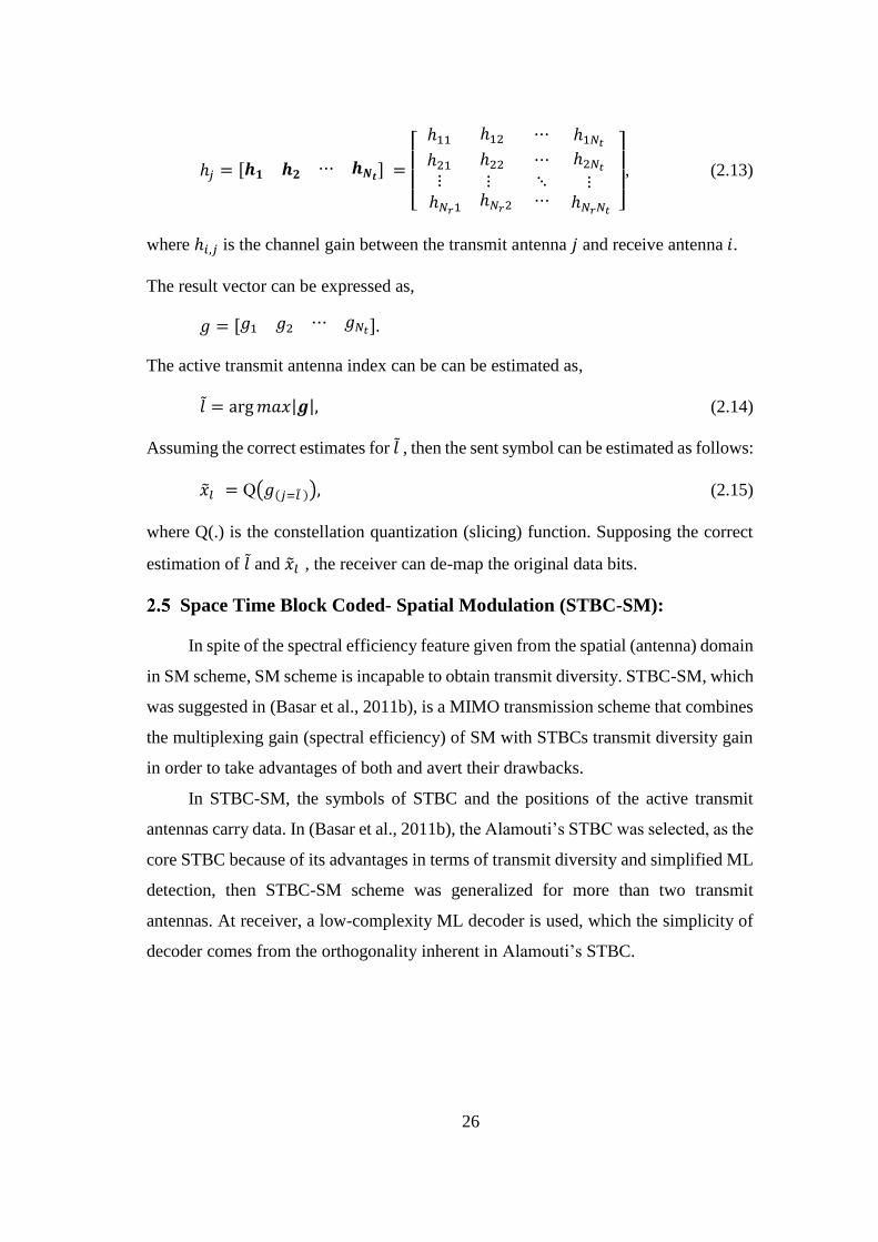
The mapping rule for 2 bits/s/Hz transmission is demonstrated by Table (2.2) for
codebooks of (2.16) and BPSK. The realization of any codeword is termed as a
transmission matrix. Each four input bits are split into two group, the first group (two
bits) are utilized to select the indices of the antenna pair 𝑙 whilst the second group (two
bits) selects the two BPSK symbol. If the system is generalized to 𝑀-ary signal
constellation, each codeword from the four codewords in (2.16) will have 𝑀2 different
realizations.
Figure (2.10): Block diagram of the STBC-SM transmitter
(Basar, Aygolu, Panayirci, & Poor, 2011b).
29
Table (2.2): STBC-SM mapping rule for 2 bits/s/Hz transmission using BPSK, 4
transmit antennas and Alamouti’s STBC (Basar et al., 2011b).
Input
Bits
Transmission
Matrices
Input
Bits
Transmission
Matrices
𝒳1
𝑙 = 0
0 0 0 0
0 0 0 1
0 0 1 0
0 0 1 1
[1‐1
11
00
00]
[11
‐11
00
00]
[‐1‐1
1‐1
00
00]
[‐11
‐1‐1
00
00]
𝒳2
𝑙 = 2
1 0 0 0
1 0 0 1
1 0 1 0
1 0 1 1
[00
1‐1
11
00] 𝑒𝑗𝜃
[00
11
‐1 1
00] 𝑒𝑗𝜃
[00
‐1‐1
1‐1
00] 𝑒𝑗𝜃
[00
‐1 1
‐1‐1
00] 𝑒𝑗𝜃
𝑙 = 1
0 1 0 0
0 1 0 1
0 1 1 0
0 1 1 1
[00
00
1‐1
11]
[00
00
11
‐11]
[00
00
‐1‐1
1‐1]
[00
00
‐11
‐1‐1]
𝑙 = 3
1 1 0 0
1 1 0 1
1 1 1 0
1 1 1 1
[11
00
00
1‐1] 𝑒𝑗𝜃
[‐11
00
00
11] 𝑒𝑗𝜃
[ 1‐1
00
00
‐1‐1] 𝑒𝑗𝜃
[‐1‐1
00
00
‐1 1] 𝑒𝑗𝜃
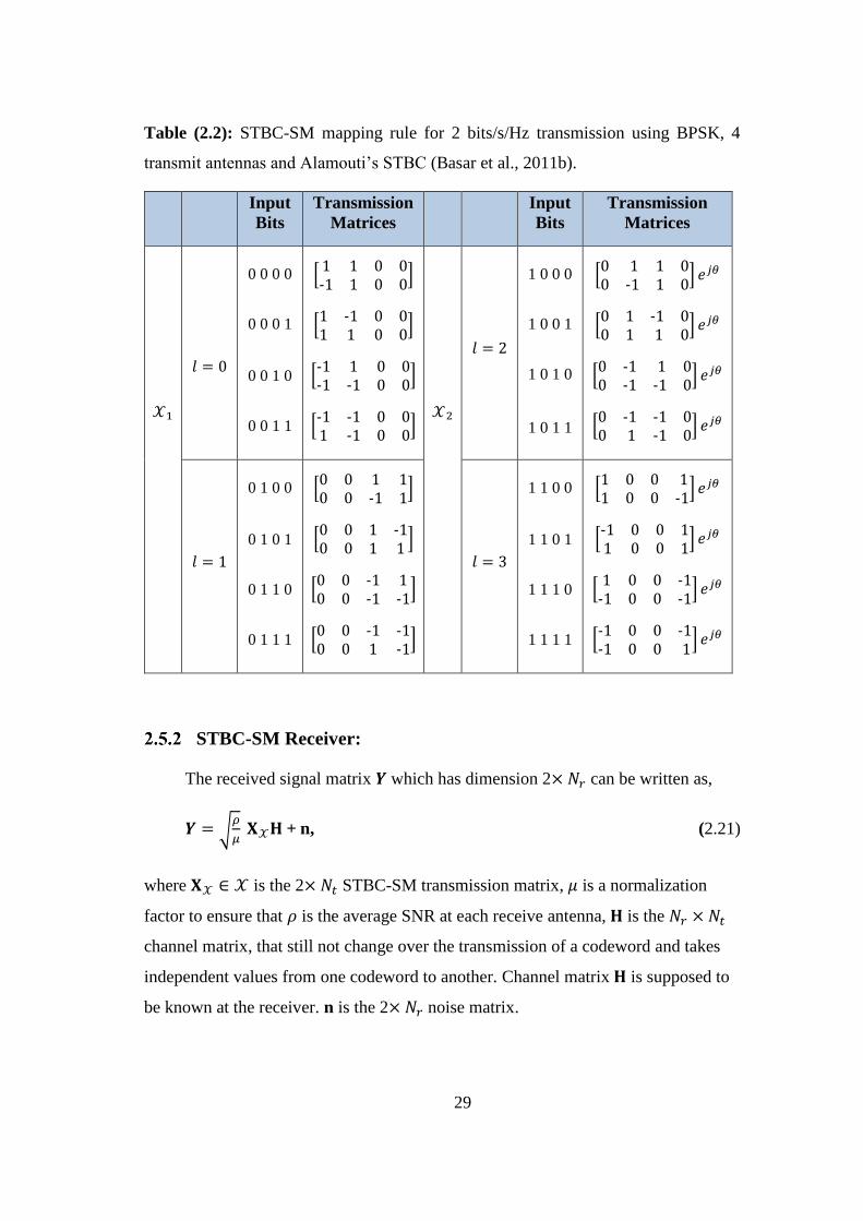
STBC-SM Receiver:
The received signal matrix 𝒀 which has dimension 2× 𝑁𝑟 can be written as,
𝒀 = √𝜌
𝜇 𝐗𝒳𝐇 + n, (2.21)
where 𝐗𝒳 ∈ 𝒳 is the 2× 𝑁𝑡 STBC-SM transmission matrix, 𝜇 is a normalization
factor to ensure that 𝜌 is the average SNR at each receive antenna, 𝐇 is the 𝑁𝑟 × 𝑁𝑡
channel matrix, that still not change over the transmission of a codeword and takes
independent values from one codeword to another. Channel matrix 𝐇 is supposed to
be known at the receiver. n is the 2× 𝑁𝑟 noise matrix.

30
Assume 𝑁𝑡 transmit antennas are used and the total number of STBC-SM
codewords is 𝑐, then for 𝑀-ary signal constellation we can construct 𝑐𝑀2 different
transmission matrices.
For ML decoder, we will search over all 𝑐𝑀2 transmission matrices and select
which one that minimizes the following metric:
�̃�𝒳 = arg min𝐗𝒳∈𝒳
‖ 𝒀 − √𝜌
𝜇 𝐗𝒳𝐇 ‖
2
. (2.22)
Because of the orthogonality of Alamouti’s STBC, the minimization of (2.22)
can be simplified. The decoder can evolve the embedded data symbol vector from
(2.21) and obtain the following equivalent channel model:
𝐲 = √𝜌
𝜇 𝓗𝒳 [
𝑠1𝑠2] + n, (2.23)
where 𝓗𝒳 is the 2𝑁𝑟 × 2 equivalent channel matrix of the Alamouti coded-SM
scheme, which has 𝑐 different realizations with respect to the STBC-SM codewords.
𝓗𝒳(𝑖, 𝑗, 𝜃) =
[ ℎ1,𝑖 𝜃 ℎ1,𝑗 𝜃
ℎ1,𝑗∗ 𝜃∗ −ℎ1,𝑖
∗ 𝜃∗
ℎ2,𝑖 𝜃 ℎ2,𝑗 𝜃
ℎ2,𝑗∗ 𝜃∗ −ℎ2,𝑖
∗ 𝜃∗
⋮ℎ𝑁𝑟,𝑖 𝜃 ℎ𝑁𝑟,𝑗 𝜃
ℎ𝑁𝑟,𝑗∗ 𝜃∗ −ℎ𝑁𝑟,𝑖
∗ 𝜃∗]
,
where 𝑖 and 𝑗 are the indices of the two Alamouti transmitting antennas and 𝜃 is the
optimized rotation angle that maximize 𝛿𝑚𝑖𝑛(𝒳) in (2.19). 𝐲 and n represent the
2𝑁𝑟 × 1 received signal and noise vectors, respectively. The columns of 𝓗𝒳 are
orthogonal to each other for all cases because of the orthogonality of Alamouti’s
STBC. Therefore, no ICI happens in STBC-SM scheme as in the SM case.
We have 𝑐 equivalent channel matrices 𝓗𝑙 , 0 ≤ 𝑙 ≤ 𝑐 − 1, and for the 𝑙𝑡ℎ
combination, the receiver determines the ML estimates of 𝑠1and 𝑠2 using the
decomposition as follows resulting from the orthogonality of ℎ𝑙,1 and ℎ𝑙,2:

31
s̃1,𝑙 = argmins1∈𝛾
‖ 𝒚 − √𝜌
𝜇 ℎ𝑙,1 s1 ‖
2
,
s̃2,𝑙 = argmins2∈𝛾
‖ 𝒚 − √𝜌
𝜇 ℎ𝑙,2 s2 ‖
2
, (2.24)
where 𝓗𝑙 = [ℎ𝑙,1 ℎ𝑙,2], 0 ≤ 𝑙 ≤ 𝑐 − 1 and ℎ𝑙,𝑗 , 𝑗 = 1,2, is a 2𝑁𝑟 × 1 column vector.
The associated minimum ML metrics 𝑚𝑙,1 and 𝑚𝑙,2 for 𝑠1and 𝑠2 are:
𝑚𝑙,1 = mins1∈𝛾
‖ 𝒚 − √𝜌
𝜇 ℎ𝑙,1 s1 ‖
2
,
𝑚𝑙,2 = mins2∈𝛾
‖ 𝒚 − √𝜌
𝜇 ℎ𝑙,2 s2 ‖
2
, (2.25)
The summation 𝑚𝑙 = 𝑚𝑙,1 +𝑚𝑙,2, 0 ≤ 𝑙 ≤ 𝑐 − 1 gives the total ML metric for the
𝑙𝑡ℎcombination. The receiver makes a decision by selecting the minimum antenna
combination metric as 𝑙 = argmin𝑙𝑚𝑙 for which (s̃1 , s̃2) = (s̃1,𝑙 , s̃2,𝑙). As result, the
total number of ML metric calculations in (2.22) is decreased from 𝑐𝑀2to 2𝑐𝑀,
yelding a linear decoding complexity (Basar et al., 2011b). Then the estimated symbols
(s̃1 , s̃2) and estimated antenna pairs 𝑙 are used to recover the input bits using
demapping process depending on the look-up table utilized at the transmitter.
The block diagram of STBC-SM receiver is illustrated in Figure (2.11),
Figure (2.11): Block diagram of STBC-SM receiver
(Basar et al., 2011b).

32
Simulation Results:
The simulation results for the STBC-SM with variable numbers of transmit
antennas and the comparison with many systems such as SM, V-BLAST, rate ¾
OSTBC for four transmit antennas and Alamoutiʼs STBC were presented in (Basar et
al., 2011b). The BER performance versus the average SNR per receive antenna for
these schemes was studied for different spectral efficiencies. All performance
comparisons are measured at a BER value of 10−5 and four receive antennas.
In Figure (2.12), the BER curves of STBC-SM (𝑁𝑡 = 4 and QPSK), OSTBC
(𝑁𝑡 = 4 and 16-QAM), Alamouti’s STBC (𝑁𝑡 = 4 and 8-QAM), SM (𝑁𝑡 = 4 and
BPSK) and V-BLAST (𝑁𝑡 = 3 and BPSK) are evaluated for 3 bits/s/Hz transmission,
respectively. STBC-SM exhibits a 2.8 dB, 3.4 dB, 3.8 dB and 5.1 dB SNR gains over
OSTBC, Alamouti’s STBC, SM and V-BLAST, respectively.
Figure (2.12): BER performance at 3 bits/s/Hz for STBC-SM, OSTBC, Alamouti’s
STBC, SM and V-BLAST schemes (Basar, Aygolu, Panayirci, & Poor, 2011b).

33
Super Orthogonal Space Time Trellis- Spatial Modulation (SOTC-
SM):
SOTC-SM is a new type of STTCs which was introduced in (Başar et al., 2012).
In SOTC-SM method, the set partitioning is applied on the super set of STBC-SM
codewords, then these codewords are assigned to the branches diverged from different
trellis states. The enhancement in the coding gain as well as getting the full diversity
order can be achieved by investing the advantages of STBC, SM and trellis codes.
Systematic construction methods and the simplified ML detection were presented for
the SOTC-SM method in (Başar et al., 2012).
The set partitioning operation for STBC-SM transmission
codewords:
For an orthogonal STBC-SM codeword 𝑿, the set partitioning is applied on the
realization matrices of the codeword 𝑿 to find subgroups like 𝑿𝑖 , 𝑿𝑖𝑗 or 𝑿𝒊𝑗𝑘, where
𝑖, 𝑗, 𝑘 ∈ {1 2}, with gradually larger minimum CGDs (Jafarkhani, 2005).
The minimum CGD of an STBC-SM codeword, considering that 𝐶𝑖 and 𝐶𝑗 are
the all possible realizations of this codeword, is evaluated as:
𝛿𝑚𝑖𝑛 = min𝐶𝑖 ,𝐶𝑗
𝑑𝑒𝑡(𝐶𝑖 − 𝐶𝑗)𝐻(𝐶𝑖 − 𝐶𝑗) (2.26)
Example: For Alamoutiʼs STBC and four transmit antennas, the STBC-SM codewords
are defined as,
𝑿𝑎=[ s1 s2 0 0‐s2* s1
* 0 0] , 𝑿𝑏=[
0 s1 s2 0
0 ‐s2* s1
* 0],
𝑿𝑐=[0 0 s1 s20 0 ‐s2
* s1*] , 𝑿
𝑑=[s1 0 0 s2‐s2* 0 0 s1
*], (2.27)
The set partitioning will be done for the four STBC-SM codewords in (2.27), the
codeword set in (2.27) also called super set. The set partitioning of the codeword 𝑿𝑎
with QPSK, 8-PSK and 16-QAM signal constellations is shown in Figure (2.13).

34
As shown in Figure (2.13), the index of the constellations symbol 𝑒𝑗(2𝜋/𝑀)(𝑎−1)
is indicated by 𝑎 ∈ {1 ,2, … ,𝑀}. As we move down to the lower levels of the tree, the
CGD increases. In the same manner, we can apply the set partitioning on remaining
three codewords (𝑿𝑏 , 𝑿𝑐 , 𝑿𝑑) that use different antenna combinations. After the set
partitioning process, the distinct STBC-SM codewords will be assigned to the
transions diverging from distinct states.
For 𝑚 bits/s/Hz transmission, there are 2𝑚𝑇branches outing from each state
when a 𝑇 × 𝑁𝑡 STBC is used, where 𝑇 is the number of channel uses and 𝑁𝑡 is the
number of transmit antennas, respectively. In (Başar et al., 2012), two different
construction methods for trellis code were introduced as follows:
1. For trellis code with 𝑆-states, we need 𝑆 distinct STBC-SM codewords. Each
codeword is assigned to only one individual state from the total number of states 𝑆.
The subsets resulting from the set partitioning for each codeword are assigned to
the branches diverging from the corresponding state.
2. For trellis code with 𝑆-states, we need 𝑆/2 different STBC-SM codewords and in a
systematic arrangement, the subsets of these codewords are assigned to the
branches emerging from different states.
Figure (2.13): STBC-SM codewords set partitioning for QPSK, 8-PSK and
16-QAM. Constellations (Başar et al., 2012).

35
𝑆 × 𝑆 state transition matrices for distinct numbers of states are illustrated in
table (2.3), with two construction techniques.
Table (2.3): Trellis state transition matrices for SOTC-SM schemes with subsets
assigned to parallel transitions (Başar et al., 2012).
State Matrix Construction
technique
2 [𝑿1𝑎 𝑿2
𝑎
𝑿1𝑏 𝑿2
𝑏] First
4
[ 𝑿11𝑎 𝑿12
𝑎
𝑿11𝑏 𝑿12
𝑏
𝑿11𝑐 𝑿12
𝑐
𝑿11𝑑 𝑿12
𝑑
𝑿21𝑎 𝑿22
𝑎
𝑿21𝑏 𝑿22
𝑏
𝑿21𝑐 𝑿22
𝑐
𝑿21𝑑 𝑿22
𝑑 ]
First
8
[ 𝑿11𝑎 𝑿12
𝑎
𝟎 𝟎𝑿11𝑐 𝑿12
𝑐
𝟎 𝟎
𝑿21𝑎 𝑿22
𝑎
𝟎 𝟎𝑿21𝑐 𝑿22
𝑐
𝟎 𝟎
𝟎 𝟎𝑿11𝑏 𝑿12
𝑏
𝟎 𝟎𝑿11𝑑 𝑿12
𝑑
𝟎 𝟎𝑿21𝑏 𝑿22
𝑏
𝟎 𝟎𝑿21𝑑 𝑿22
𝑑
𝑿21𝑎 𝑿22
𝑎
𝟎 𝟎𝑿21𝑐 𝑿22
𝑐
𝟎 𝟎
𝑿11𝑎 𝑿12
𝑎
𝟎 𝟎𝑿11𝑐 𝑿12
𝑐
𝟎 𝟎
𝟎 𝟎𝑿21𝑏 𝑿22
𝑏
𝟎 𝟎𝑿21𝑑 𝑿22
𝑑
𝟎 𝟎𝑿11𝑏 𝑿12
𝑏
𝟎 𝟎𝑿11𝑑 𝑿12
𝑑 ]
Second
8
[ 𝑿111𝑎 𝑿112
𝑎
𝑿111𝑏 𝑿112
𝑏
𝑿111𝑐 𝑿112
𝑐
𝑿111𝑑 𝑿112
𝑑
𝑿121𝑎 𝑿122
𝑎
𝑿121𝑏 𝑿122
𝑏
𝑿121𝑐 𝑿122
𝑐
𝑿121𝑑 𝑿122
𝑑
𝑿211𝑎 𝑿212
𝑎
𝑿211𝑏 𝑿212
𝑏
𝑿211𝑐 𝑿212
𝑐
𝑿211𝑑 𝑿212
𝑑
𝑿221𝑎 𝑿222
𝑎
𝑿221𝑏 𝑿222
𝑏
𝑿221𝑐 𝑿222
𝑐
𝑿221𝑑 𝑿222
𝑑
𝑿111𝑒 𝑿112
𝑒
𝑿111𝑓
𝑿112𝑓
𝑿111𝑔
𝑿112𝑔
𝑿111ℎ 𝑿112
ℎ
𝑿121𝑒 𝑿122
𝑒
𝑿121𝑓
𝑿122𝑓
𝑿121𝑔
𝑿122𝑔
𝑿121ℎ 𝑿122
ℎ
𝑿211𝑒 𝑿212
𝑒
𝑿211𝑓
𝑿212𝑓
𝑿211𝑔
𝑿212𝑔
𝑿211ℎ 𝑿212
ℎ
𝑿221𝑒 𝑿222
𝑒
𝑿221𝑓
𝑿222𝑓
𝑿221𝑔
𝑿222𝑔
𝑿221ℎ 𝑿222
ℎ ]
First
where the submatrix at the row 𝑖 and column 𝑗, 𝑖, 𝑗 = 1, . . . , 𝑆 refers to the subset
assigned to the parallel branches emerging from the state 𝑖 and merging to the state 𝑗.
The no transition between two states is represented by a zero matrix 𝟎, and (𝑿𝑎, 𝑿𝑏,
… , 𝑿ℎ) refer to the STBC-SM codewords which have different antenna combinations.

36
SOTC-SM Encoding:
For the case of Alamoutiʼs STBC, there are 22𝑚 branches emerging from each
state where 𝑚 = log2(𝑀). In SOTC-SM transmitter, a 2𝑚 input bits choose the
corresponding transition out of 22𝑚 transitions on the trellis diverging from a given
state. Each transition corresponds to the transmission of two symbols 𝑠1and 𝑠2 in two
symbol time durations from a pair of transmitting antennas which is determined by
STBC-SM codewords. Figure (2.14) demonstrates the trellis diagram of the 4-state
SOTC-SM scheme.
SOTC-SM Decoding:
The received signal matrix 𝒚 which has dimension 2× 𝑁𝑟 can be written as,
𝒚 = 𝑿𝒉 +n, (2.28)
where 𝑿 is the 2× 𝑁𝑡 transmission matrix, which is transmitted over two symbol time
durations. 𝒉 is the 𝑁𝑟 × 𝑁𝑡 channel matrix, that is supposed to be known at the
receiver, and n is the 2×𝑁𝑟 white Gaussian noise matrix.
The Viterbi decoder is used for ML decoding and it decides the most likely
transmitted path. At each state transition, the Viterbi decoder finds the most probably
transition with the minimum branch metric amongst all parallel branches (Başar et al.,
2012). Because of the orthogonality of Alamouti’s STBC, the total number of metric
Figure (2.14): Four-state SOCT-SM scheme (Başar, Aygölü,
Panayırcı, & Poor, 2012).

37
calculations can be decreased. The embedded data symbol vector can be extracted by
the decoder from Equation (2.28) and getting the following equivalent channel model:
𝐲𝒆𝒒 = 𝓗𝑖 [𝑠1𝑠2] +n (2.29)
where 𝓗𝑖 = [ℎ1𝑖 ℎ2
𝑖 ] is the 2𝑁𝑟 × 2 channel matrix of SOTC-SM and index 𝑖 ∈
{𝑎, 𝑏, 𝑐, … } determines the corresponding antenna combination. 𝐲 is the 2𝑁𝑟 × 1
received signal and n is 2𝑁𝑟 × 1 noise matrix. The ℎ1𝑖 and ℎ2
𝑖 are the columns of 𝓗𝑖
and they are orthogonal to each other for all cases, where the orthogonality is derived
from the Alamouti’s STBC.
The decision metric M𝑗𝑖(𝑠𝑗) for 𝑗 = 1,2 can separated as:
M𝑗𝑖(𝑠𝑗) = ‖ 𝐲𝒆𝒒 − ℎ𝑗
𝑖 s𝑗 ‖2 (2.30)
Then by calculating M1𝑖 (𝑠1) and M2
𝑖 (𝑠2) for all values of 𝑠1and 𝑠2 and reserving the
resulting metrics, and employing them for distinct subsets of the same partitioning
level, the decoder complexity is reduced significantly (Başar et al., 2012).
Simulation Results:
The error performance of the SOTC-SM scheme with different structures is
compared to the SOSTTCs, and the spatial modulation trellis code SM-TC error
performances.
SOSTTC is a systematically designed type of (STTCs) that merges the STBCs
with trellis codes using the concept of set partitioning in order to obtain coding gain
larger than the conventional STTCs with low decoding complexity (Jafarkhani &
Seshadri, 2003).
SM-TC is a new trellis code design for spatial modulation, that exploits coding
gain of trellis code for SM. In (Basar, Aygolu, Panayirci, & Poor, 2011a), in terms of
BER and frame error rate (FER) performance, it was shown that the SM-TC achieves
an important improvements than the STTCs with reduction in decoding complexity.
BER and FER performances versus the average SNR per receive antenna for
these schemes was evaluated and shown in Figure (2.15) and Figure (2.16) for different
numbers of trellis states and spectral efficiencies.

38
In Figure (2.15), a significant enhancement is accomplished by the SOTC-SM
scheme in comparison to the SM-TC scheme which uses the same number of transmit
antennas and the same number of states. The 4-state SOTC-SM scheme provides SNR
gains of 2.6 and 1.3 dB over the 4-state SM-TC scheme for 𝑁𝑟 =1 and 2, respectively,
whilst the 8-state SOTC-SM scheme provides SNR gains of 1.5 and 0.4 dB over the
8-state SM-TC scheme for 𝑁𝑟 =1 and 2, respectively.
In Figure (2.16), the FER performance of the SOTC-SM is better than the
FER performance of the SOSTTCs for the same number of active transmit antennas
during transmission. The 4-state SOTC-SM scheme provides SNR gains of 2.2 and
1.6 dB over the 4-state SOSTTC scheme for 𝑁𝑟 =1 and 2, respectively, whilst the 8-
state-I SOTC-SM scheme provides SNR gains of 2.1 and 1.7 dB over the 8-state
SOSTTC scheme for 𝑁𝑟 =1 and 2, respectively.
Figure (2.15): BER performance for 4- and 8-state SOTC-SM
and SM-TC schemes (2 bits/s/Hz) (Başar et al., 2012).

39
Antenna Selection (AS) for MIMO systems:
MIMO system with 𝑁𝑡 transmit antennas and 𝑁𝑟 receive antennas needs 𝑁𝑡 full
RF chains in the transmitter and 𝑁𝑟 complete RF chains in the receiver. Each transmit
antenna element needs an RF chain that consists of a digital-to analog converter, a
frequency up-converter and a power amplifier, and each receive antenna element
requires an RF chain that consists of a low noise amplifier, frequency down-converter
and analog-to-digital converter. Therefore, the complexity of MIMO system will
increase as well as the cost of implementation will also increase.
One effective way to decrease the number of RF chains is AS. It mitigates the
complexity of MIMO systems. The main goal of AS is to implement more antennas
than RF chains and use only a subset of them but maintaining the advantages of
MIMO. AS can be employed both in the transmitter and in the receiver.
In TAS, the best 𝐿𝑡 out of 𝑁𝑡 antennas are selected. Similarly, in RAS, the best
𝐿𝑟 out of 𝑁𝑟 antennas are selected. In MIMO systems, to apply TAS, we will select
some columns from the channel matrix. Similarly, to apply RAS, we will select some
rows from the channel matrix.
Figure (2.16): FER performance for 2-, 4- and 8-state SOTTC
schemes (3 bits/s/Hz) (Başar et al., 2012).

40
The block diagram of AS with MIMO systems is shown in Figure (2.17).
The RF switch is controlled by the selection criteria implemented at the receiver.
In TAS case, the receiver tells the transmitter which the indices of the 𝐿𝑡 out of 𝑁𝑡
transmit antennas to be utilized at each frame through an existing a limited feedback
link between the receiver and the transmitter. As only the indices of the selected
antennas are to be fed back, few bits are required. The main drawback of TAS is the
need of a new bandwidth and different frequency for the feedback link, but compared
to the benefits that can be achieved from the TAS (full diversity gain and full capacity)
with a low computational complexity and reduction in the hardware complexity, this
drawback can be overlooked.
The performance of AS has been discussed from several aspects like capacity
for spatial multiplexing systems, and diversity order and coding gain for STC systems.
For the variety of MIMO techniques, the AS achieves the full diversity inherent in the
system at the expense of a small loss in array gain in comparison to a full complexity
system (Tsoulos, 2006). Many AS algorithms have been developed in the last decade.
We can classify the AS algorithms into two main categories: the first is optimal AS
algorithms (high computational complexity), and the second is sub-optimal AS
algorithms (low computational complexity).
The optimal AS algorithm is the method that uses a comprehensive search of all
possible combinations to find the one group that provides the best SNR (for diversity)
or capacity (for spatial multiplexing). Therefore, the optimal AS algorithms require
high computational processes at any change in channel, which in turn leads to the
difficulty of implementing these algorithms practically (Molisch, Win, Choi, &
Winters, 2005)
Figure (2.17): Block diagram of AS with MIMO system (Tsoulos, 2006).

41
Since the optimal AS schemes suffer from practical limitations due to the high
computational complexity, we use the sub-optimal AS algorithms due to their lack of
computational complexity and ease of implementation.
In our thesis, we will focus on two sub-optimal AS Algorithms for DSM, STBC-
SM and SOTC-SM schemes. The first algorithm is capacity optimized AS (COAS)
and the second is AS based on Amplitude and Antenna Correlation (A-C-AS).
Capacity Optimized Antenna Selection (COAS):
COAS algorithm, also called norm-based antenna selection, is AS algorithm that
selects a sub group of antennas (𝐿𝑡 / 𝐿𝑟) which correspond to the maximum channel
amplitudes (columns or rows of channel matrix) from the total number of transmit
antennas 𝑁𝑡 or receive antennas 𝑁𝑟 . The results of many researches proved that the
COAS algorithm was capable of enhancing the error performance of variety MIMO
systems, whilst maintaining a very low computational complexity.
Transmit Antenna Selection (TAS) based on COAS:
Consider the channel matrix 𝐇 has a size of 𝑁𝑟 ×𝑁𝑡. The COAS algorithm can
be applied as following:
Step 1: Calculate the Frobenius norm of each column vector in the channel matrix 𝐇:
‖ℎ𝑖‖𝐹2 (2.31)
where 𝑖 ∈ [1: 𝑁𝑡]
Step 2: Arrange in descending order the column vectors of:
HA = [‖ℎ1‖𝐹2 ≥ ‖ℎ2‖𝐹
2 ≥ ⋯ ≥ ‖ℎ𝑁𝑡‖𝐹2] (2.32)
Step 3: Choose the highest 𝐿𝑡 channel gain vectors to form the 𝐿𝑡 × 𝑁𝑟 channel gain
matrix H𝑇𝑥_𝑠𝑒𝑙.
Receive Antenna Selection (RAS) based on COAS:
Step 1: Calculate the Frobenius norm of each row vector in matrix 𝐇:
‖ℎ𝑗‖𝐹2 (2.33)
where 𝑗 ∈ [1:𝑁𝑟]
Step 2: Arrange in descending order the row vectors of 𝐇:

42
HA = [‖ℎ1‖𝐹2 ≥ ‖ℎ2‖𝐹
2 ≥ ⋯ ≥ ‖ℎ𝑁𝑟‖𝐹2] (2.34)
Step 3: Choose the highest 𝐿𝑟 channel gain vectors to form the 𝑁𝑡 × 𝐿𝑟 channel gain
matrix H𝑅𝑥_𝑠𝑒𝑙.
Antenna selection based on Amplitude and Antenna Correlation
(A-C- AS) (Pillay & Xu, 2014):
A-C-AS is AS algorithm based on the combination of two selection criteria,
channel amplitude and antenna correlation. The correlation-based algorithm was
introduced in (Molisch et al., 2005). The principle behind correlation-based algorithm
is that a transmitter or receiver chooses one pair of two antennas who are most highly
correlated, then, the antenna with lower channel gain is rejected. The transmitter or the
receiver repeats selecting a pair and rejecting one antenna until there are 𝐿𝑡 or 𝐿𝑟
antennas remained, so that the remaining 𝐿𝑡 or 𝐿𝑟 antennas have the lowest correlation
and the largest channel gains as possible. TAS based on amplitude and antenna
correlation (A-C-TAS) was first suggested for SM by (Pillay & Xu, 2014). This
scheme selects 𝐿𝑡 + 1 transmit antennas from 𝑁𝑡 total transmit antennas that
correspond to the largest channel amplitudes then calculates the correlation for all
(Lt+12) pairs. The transmit antenna pair that corresponds to the highest correlation is
selected and the antenna that has smaller channel gains within the selected pair is
rejected. A-C-AS scheme has shown a significant improvement in BER at low
computational complexity. The smaller the correlation between transmit antennas, the
better the overall system performance (Zhou, Ge, & Lin, 2014) .
In A-C-TAS algorithm, where Lt ≥ 2, we will select 𝑁𝑐 = 𝐿𝑡 + 1 from 𝑁𝑡 total
transmit antennas that correspond to the maximum channel amplitudes, then the
correlation for all (𝑁𝑐2) pairs are calculated. The transmit antenna pair that corresponds
to the highest correlation is selected and the antenna that has smaller channel gains
within the selected pair is rejected. Similarly, we can apply A-C-AS algorithm at the
receiver side for Lr ≥ 2.

43
Transmit Antenna Selection (TAS) based on A-C (A-C-TAS):
Consider the channel 𝐇 has a size of 𝑁𝑟 ×𝑁𝑡. The A-C-TAS algorithm can be
applied as following,
Step 1: Calculate the Frobenius norm of each column vector in the channel matrix 𝐇:
‖ℎ𝑖‖𝐹2 (2.35)
where 𝑖 ∈ [1: 𝑁𝑡]
Step 2: Choose the 𝑁𝑐 = 𝐿𝑡 + 1 transmit antennas that correspond to the highest
channel amplitudes.
H𝑁𝑐 = [‖ℎ1‖𝐹2 ≥ ‖ℎ2‖𝐹
2 ≥ ⋯ ≥ ‖ℎ𝑁𝑐‖𝐹2] (2.36)
Step 3: Determine all possible enumerations of the channel gain vector pairs. The total
number of possible vector pairs is given by 𝑁𝐴 = (𝑁𝑐2) . Each pair will have the form
(ℎ𝑥 , ℎ𝑦).
Step 4: Calculate the angle of correlation θ between both vectors of a vector pair. For
each vector pair θ can be calculated as:
θ𝑧 = cos−1 (
|ℎ𝑥𝐻ℎ𝑦|
‖ℎ𝑥‖𝐹 ‖ℎ𝑦‖𝐹) (2.37)
where 𝑧 ∈ [1:𝑁𝐴]
The angle of correlation for each pair is stored in 𝐴θ:
𝐴θ = [θ1 θ2… θ𝑁𝐴]
Step 5: Choose the largest correlation pair which has the smallest angle and reject the
smaller of the two channel gain vectors. This forms the 𝐿𝑡 ×𝑁𝑟 channel gain matrix
H𝑇𝑥_𝑠𝑒𝑙.
Receive Antenna Selection (RAS) based on A-C (A-C-RAS):
Step 1: Calculate the Frobenius norm of each row vector in the channel matrix 𝐇
‖ℎ𝑗‖𝐹2 (2.38)
where 𝑗 ∈ [1:𝑁𝑟]
The steps from 2 to 5 are identical to the preceding TAS scheme. Then we can form
the 𝑁𝑡 × 𝐿𝑟 channel gain matrix H𝑅𝑥_𝑠𝑒𝑙.

44
Computational Complexity for the two AS algorithms:
We will evaluate the computational complexity for both AS algorithms in terms
of the number of real multiplcations (RM) and real addition (RA). Note that, a complex
multiplication is equivalent to 4 RM and 2 RA, ((a + jb) ∗ (c + jd) = (a ∗ c − b ∗ d) + j
(b ∗ c + a ∗ d)), while a complex addition is equivalent to 2 RA, ((a + jb) + (c + jd) =
(a + c) + j (b + d)).
Computational Complexity for COAS-TAS:
The required numbers of real operations to compute (2.30) is given by:
𝓒𝐂𝐎𝐀𝐒−𝐓𝐀𝐒 = 𝑁𝑡(8 𝑁𝑟 − 2) (2.39)
The Frobenius norm in (2.30) needs 𝑁𝑟 complex multiplication and (𝑁𝑟 − 1)
complex addition for each column vector in the channel matrix 𝐇. Then the total
number of real operations for each column equals,
𝑁𝑟 (4 RM + 2 RA) + (𝑁𝑟 − 1)(2 RA) + 1 RM = 𝑁𝑟 (4 RM) + 𝑁𝑟 (4 RA) – 2 RA =
(8 𝑁𝑟 – 2)
These operations are done 𝑁𝑡 times.
Computational Complexity for CO-RAS:
The required numbers of real operations to compute (2.32) is given by:
𝓒𝐂𝐎𝐀𝐒−𝐑𝐀𝐒 = 𝑁𝑟(8 𝑁𝑡 − 2) (2.40)
The Frobenius norm in (2.32) needs 𝑁𝑡 complex multiplication and (𝑁𝑡 − 1)
complex addition for each row vector in the channel matrix 𝐇. Then the total number
of real operations for each row equals,
𝑁𝑡 (4 RM + 2 RA) + (𝑁𝑡 − 1)(2 RA) + 1 RM = 𝑁𝑡 (4 RM) + 𝑁𝑡 (4 RA) – 2 RA =
(8 𝑁𝑡 – 2)
These operations are done 𝑁𝑟 times.

45
Computational Complexity for A-C-TAS:
The required numbers of real operations to compute (2.34) and (2.36) is given
by:
𝓒𝐀−𝐂−𝐓𝐀𝐒 = 𝑁𝑡(8 𝑁𝑟 − 2) + (𝑁𝑐2) (24 𝑁𝑟 –2) (2.41)
The Frobenius norm in (2.34) needs 𝑁𝑡(8 𝑁𝑟 – 2).
The numerator in (2.36) requires 𝑁𝑟 complex multiplication + (𝑁𝑟 − 1) complex
addition and 2 RM + 1 RA for evaluating the absolute value, so the total number of
real operations for numerator equals,
𝑁𝑟 (4 RM + 2 RA) + (𝑁𝑟 − 1)(2 RA) + 2 RM + 1 RA = 𝑁𝑟 (4 RM) + 𝑁𝑟 (4 RA) – 2
RA + 2 RM + 1 RA = (8 𝑁𝑟 + 1).
In the denumerator of (2.36), each Frobenius norm requires 𝑁𝑟 complex
multiplication, (𝑁𝑟 − 1) complex addition and the mulpication of the two norms
requires 1 RM, so the total number of real operations for denumerator equals,
2 (𝑁𝑟 (4 RM + 2 RA) + (𝑁𝑟 − 1)(2 RA)) + 1 RM = 𝑁𝑟 (8 RM) + 𝑁𝑟 (8 RA) – 4 RA
+ 1 RM = (16 𝑁𝑟 – 3)
So, the the total number of real operations in (2.36) equals (8 𝑁𝑟 +1) + (16 𝑁𝑟 – 3) =
(24 𝑁𝑟 – 2)
These operations are done (𝑁𝑐2) times.
Computational Complexity for A-C-RAS:
The required numbers of real operations to compute (2.37) and (2.36) is given
by:
𝓒𝐀−𝐂−𝐑𝐀𝐒 = 𝑁𝑟(8 𝑁𝑡 − 2) + (𝑁𝑐2) (24𝑁𝑡 − 2) (2.42)
The total number of real operations in (2.37) equals 𝑁𝑟 (8 𝑁𝑡 – 2).
The total number of real operations in (2.36) equals (8 𝑁𝑡+1) + (16 𝑁𝑡 – 3) = (24 𝑁𝑡 –
2). These operations are done (𝑁𝑐2) times.

46
Summary:
In this chapter, the main topics needed in this thesis were clarified and reviewed.
These topics include diversity, Space Time Coding, Space Time Trellis Coding
(STTC), Space Time Block Coding (STBC), Spatial Modulation (SM), Space Time
Block coded- Spatial Modulation (STBC-SM), Super Orthogonal Space Time Trellis-
Spatial Modulation (SOTC-SM), and Antenna Selection (AS) for MIMO system.

47
Chapter 3
Antenna Selection for
Double Spatial
Modulation (DSM)

48
Chapter 3
Antenna Selection for Double Spatial Modulation (DSM)
Introduction:
DSM is a new transmission technique which has been suggested for MIMO
communication systems. It was suggested to enhance the spectral efficiency of the
classical SM by raising the number of active transmitting antennas (Yigit & Basar,
2016). In this chapter and in order to get better performance for the DSM scheme, the
AS techniques are applied. The two sub-optimal AS algorithms COAS and A-C-AS,
which were mentioned in (chapter2, section 2.7.1and section 2.7.2), are applied to
DSM. MATLAB simulation results of the two sub-optimal AS algorithms with DSM
are presented.
Double Spatial Modulation (DSM):
In MIMO systems, spatial multiplexing method is used to cover the need of
higher data rates in wireless communications by employing all multiple transmitting
antennas in order to convey the data simultaneously.(Goldsmith, 2005)
The V-BLAST scheme is an example of spatial multiplexing method (Foschini,
1996). This transmission method achieves high data rate, but it suffers from ICI and
high complexity at receiver.
As it was mentioned in (chapter2, section 2.4), SM scheme overcomes on the
problem of ICI which is totally avoided, this results in a low receiver complexity.
Although the SM improved the spectral efficiency of the MIMO systems but did not
achieve the degree of improvement achieved by the V-BLAST scheme. Therefore, the
SM has been improved through several schemes such as double spatial modulation
(DSM) scheme in order to enchance the spectral efficiency of the classical SM (Yigit
& Basar, 2016).
In DSM scheme, a transmission vector is constructed by superpostion of two
independent SM transmission vectors. One of the information symbols is immediately
sent through its corresponding activated transmit antenna, whilst the second
information symbol is sent from the second actived antenna with rotation angle. This

49
rotation angle is optimized for M-QAM signal constellations to differentiate the two
distinct information symbols from each other in DSM transmission vector and
decrease the BER. The spectral efficiency of the classical SM is a half of the spectral
efficiency of the DSM scheme.
DSM Transmitter:
The input binary bits 𝑚 = log2(𝑁𝑡2𝑀2), which are the transmitted data at any
time instance, are split into two equal parts by a primary splitter, each part contains
log2(𝑁𝑡𝑀) bits, where 𝑁𝑡 and 𝑀 refer to the total number of transmitting antennas and
constellations size, respectively.
Each part selects its own information symbol and the position of active
transmitting antenna. In each part, the log2(𝑁𝑡𝑀) bits are split into two sets of bits
by a secondary splitter, the first set of bits, log2(𝑁𝑡), determines the location of an
active transmit antenna, whilst the second set of bits, log2(𝑀), determines the
corresponding transmit symbol from M-ary signal constellation.
The block diagram of DSM transmitter is illustrated in Figure (3.1),
The first active transmit antenna 𝑙1 is used to send the information symbol 𝑠1,
whilst the other active transmit antenna 𝑙2 is employed to send the information symbol
𝑠2 with rotation angle θ. The transmission vector 𝐬 of the DSM scheme, which has a
size 𝑁𝑡 × 1 can be given as,
𝒔 = {0 ⋯0 𝑠1⏟𝑙1
0 ⋯ 0 𝑠2 𝑒𝑗𝜃 ⏟ 𝑙2
0 ⋯0} (3.1)
Figure (3.1): Block diagram of DSM transmitter (Yigit & Basar, 2016).

50
Generally, the spectral efficiency of double spatial modulation DSM is given as
follow,
𝑚 = log2(𝑁𝑡2) + log2(𝑀
2) (3.2)
DSM Receiver:
The received vector 𝑦 , that has a dimension of 𝑁𝑟 × 1 , can be as,
𝑦 = 𝐇s + 𝐧
= 𝒉𝒍𝟏s1 + 𝒉𝒍𝟐s2𝑒𝑗𝜃 + 𝐧, (3.3)
where 𝐇 is the channel matrix that has a size of 𝑁𝑟 × 𝑁𝑡, 𝒉𝒍𝟏 and 𝒉𝒍𝟐denote the 𝑙1th
and 𝑙2th column vectors of H, respectively, and n is the 𝑁𝑟 × 1 white Gaussian noise
vector. ML detector is used to obtain the optimum BER performance for the DSM
scheme taking into account the CSI is fully known at the receiver side. ML detector
considers all potential realizations of the antenna indices 𝑙1 and 𝑙2 and M-QAM
constellation symbols s1 and s2 to determine the antenna postions 𝑙1 and 𝑙2 together
with the information symbols s̃1 and s̃2 by computing 𝑁𝑡2𝑀2 decision metrics and
select which one that minimizes the following metric,
(s̃1 , s̃2 , 𝑙1 , 𝑙2) = arg mins1 ,s2 ,𝑙1 ,𝑙2
‖𝑦 − (𝒉𝒍𝟏s1 + 𝒉𝒍𝟐s2𝑒𝑗𝜃)‖
2 (3.4)
The block diagram of DSM receiver is illustrated in Figure (3.2).
Figure (3.2): Block diagram of DSM receiver (Yigit & Basar, 2016).

51
Computational Complexity for DSM:
The required numbers of real operations to compute (3.4) is given by:
𝓒𝐃𝐌𝐒 = 22 𝑁𝑟 2log2(𝑀
2𝑁𝑡2) (3.5)
The ‖𝑦 − (𝒉𝒍𝟏s1 + 𝒉𝒍𝟐s2𝑒𝑗𝜃)‖
2 term in (3.4) needs 2 complex multiplication, 2
complex addition and evaluating the square needs another 1 complex multiplication.
Therefore, the total complex computational operations required are (3 complex
multiplication + 2 complex addition). Accordingly, the total real computational
operations required are 12 RM + 10 RA. These operations are done 𝑁𝑟 times and over
all possible transmitted vector combinations between transmit antennas and data
symbols 2log2(𝑀2𝑁𝑡
2).
Antenna Selection for DSM scheme:
We will apply the two AS algorithms in transmitter side, then in receiver side.
Transmit Antenna Selection (TAS) for DSM:
Consider the channel matrix 𝐇 has a size of 𝑁𝑟 ×𝑁𝑡. A best set of transmit
antennas 𝐿𝑡 are selected depending on one of the AS algorithms (COAS or A-C-AS)
and the channel matrix. The selected transmit antennas 𝐿𝑡 are used to convey the
transmission vector 𝐬 of the DSM. The block diagram of TAS for DSM and scheme is
illustrated in Figure (3.3).
Figure (3.3): The block diagram of TAS for DSM scheme.
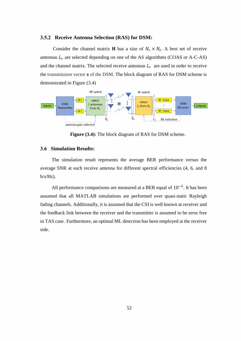
52
Receive Antenna Selection (RAS) for DSM:
Consider the channel matrix 𝐇 has a size of 𝑁𝑟 ×𝑁𝑡. A best set of receive
antennas 𝐿𝑟 are selected depending on one of the AS algorithms (COAS or A-C-AS)
and the channel matrix. The selected receive antennas 𝐿𝑟 are used in order to receive
the transmission vector 𝐬 of the DSM. The block diagram of RAS for DSM scheme is
demonstrated in Figure (3.4)
Simulation Results:
The simulation result represents the average BER performance versus the
average SNR at each receive antenna for different spectral efficiencies (4, 6, and 8
b/s/Hz).
All performance comparisons are measured at a BER equal of 10−5. It has been
assumed that all MATLAB simulations are performed over quasi-static Rayleigh
fading channels. Additionally, it is assumed that the CSI is well known at receiver and
the feedback link between the receiver and the transmitter is assumed to be error free
in TAS case. Furthermore, an optimal ML detection has been employed at the receiver
side.
Figure (3.4): The block diagram of RAS for DSM scheme.

53
Transmit Antenna Selection (TAS) for DSM:
Figure (3.5) shows the BER performance of the two sub-optimal TAS algorithms
(COAS and A-C-AS) on DSM with spectral efficiency 4 b/s/Hz, different numbers of
total transmit antennas 𝑁𝑡 and the selected transmit antennas 𝐿𝑡 equal 2. Both
algorithms have been compared to each other.
The performance of COAS-DSM and A-C-AS-DSM schemes outperform the
conventional DSM (BPSK, 𝑁𝑡 = 2) scheme with 1.5 dB and 4 dB SNR gains,
respectively, when 𝑁𝑡 = 4 . However, this gain can be further improved by increasing
𝑁𝑡. When 𝑁𝑡 is increased to 8, COAS-DSM and A-C-AS-DSM exhibit a 2.5 dB and
5.5 dB SNR gains over the classical DSM. Furthermore, at a BER of 10−5, A-C-AS-
DSM outperforms COAS-DSM by 2.5 dB and 3 dB SNR gains when 𝑁𝑡 = 4 and 8,
respectively.
It is noted that by increasing the value of 𝑁𝑡, the overall BER performance of
AS scheme will improve (BER decrease).
Figure (3.5): BER performance of TAS for DSM for 4 b/s/Hz and 𝑁𝑟 = 4.

54
Figure (3.6) illustrates the BER performance of the two sub-optimal TAS
algorithms (COAS and A-C-AS) on DSM with spectral efficiency 6 b/s/Hz, different
numbers of total transmit antennas 𝑁𝑡 and the selected transmit antennas 𝐿𝑡 equal 4.
Both algorithms have been compared to each other.
When 𝑁𝑡 = 6, the performance of COAS-DSM and A-C-AS-DSM schemes
surpasses the error performance of the conventional DSM (BPSK, 𝑁𝑡 = 4) scheme,
with an approximate SNR gain of 1.2 dB and 2.5 dB, respectively. Whilst 𝑁𝑡 is
increased to 8, COAS-DSM and A-C-AS-DSM have SNR gains of 1.8 dB and 3.3 dB
over the conventional DSM. At
At BER of 10−5, the A-C-AS-DSM outperforms COAS-DSM by 1.3 dB and
1.5 dB SNR gains when 𝑁𝑡 = 6 and 8, respectively.
It is important to note that the overall BER performance of AS scheme will
enhance (BER decrease) when the value of 𝑁𝑡 increases.
Figure (3.6): BER performance of TAS for DSM for 6 b/s/Hz and 𝑁𝑟 = 4.

55
Figure (3.7) depicts the behaviour of the two sub-optimal TAS algorithms
(COAS and A-C-AS) on DSM with spectral efficiency 8 b/s/Hz, total transmit antennas
𝑁𝑡 = 8 and the selected transmit antennas 𝐿𝑡 equal 4. Both algorithms have been
compared to each other.
As shown in Figure (3.7), a significant improvement is achieved by COAS-DSM
and A-C-AS-DSM schemes compared to the classical DSM which has the similar total
number of transmit antennas 𝑁𝑡 = 8 and the same spectral efficiency 8 b/s/Hz.
The COAS-DSM and A-C-AS-DSM schemes provides SNR gain of 0.6 dB and
1.8 dB over the conventional DSM, respectively. Accordingly, it can be said that the
COAS-DSM and A-C-AS-DSM schemes outperforms the conventional DSM scheme
provided both schemes have the identical spectral efficiency and the identical total
number of transmit antennas. Morever, at a BER of 10−5, the A-C-AS-DSM
outperforms COAS-DSM by 1.2 dB SNR gain. Also, the performance of COAS-DSM
and A-C-AS-DSM schemes outperform the conventional DSM (4-QAM, 𝑁𝑡 = 4)
scheme with 2.2 dB and 4 dB SNR gains, respectively.
Figure (3.7): BER performance of TAS for DSM for 8 bits/s/Hz and 𝑁𝑟 = 4.

56
Receive Antenna Selection (RAS) for DSM:
Figure (3.8), investigates the BER performance of the two sub-optimal RAS
algorithms (COAS and A-C-AS) on DSM scheme which has spectral efficiency 4
b/s/Hz, total receive antennas 𝑁𝑟 = 4 and the selected receive antennas 𝐿𝑟 equal 2.
Both algorithms have been compared to each other.
The performance of COAS-DSM and A-C-AS-DSM schemes shows an
improvement upon conventional DSM scheme (BPSK, 𝑁𝑟 = 2) with 3.6 dB and 8.6
dB, respectively, when 𝐿𝑟 = 2 selected from 𝑁𝑟 = 4.
At BER of 10−5, the A-C-AS-DSM outperforms COAS-DSM by 5 dB SNR gain.
The COAS-DSM and A-C-AS-DSM schemes are less hardware complexity
(two RF chains at receiver instead of 4 RF chains) than the conventional DSM ( 𝑁𝑟 =
4 with optimal ML decoder), furthermore, the two schemes are less computational
complexity compared to the conventional DSM (𝑁𝑟 = 4 with optimal ML decoder),
but the performance of COAS-DSM and A-C-AS-DSM are 9 dB and 4 dB SNR gains
worse, respectively.
Figure (3.8): BER performance of RAS for DSM for 4 b/s/Hz, 𝑁𝑡 = 2 and 𝑁𝑟 = 4.

57
Figure (3.9), illustrates the BER performance of the two sub-optimal RAS
algorithms (COAS and A-C-AS) on DSM scheme which has spectral efficiency 4
b/s/Hz, total receive antennas 𝑁𝑟 = 8 and the selected receive antennas 𝐿𝑟 equal 2.
Both of algorithms have been compared.
As shown in Figure (3.9), a considerable improvement is achieved by COAS-
DSM and A-C-AS-DSM schemes compared to the conventional DSM scheme (BPSK,
𝑁𝑟 = 2). The COAS-DSM and A-C-AS-DSM schemes provides SNR gain of 5 dB
and 10.8 dB SNR gains over the conventional DSM (BPSK, 𝑁𝑟 = 2), respectively.
At a BER of 10−5, the A-C-AS-DSM outperforms COAS-DSM by 5.8 dB SNR gain.
It is important to note that the COAS-DSM and A-C-AS-DSM schemes need
two RF chains at receiver instead of 8 RF chains, this makes the two schemes are
lower hardware complexity and computational complexity than the conventional
DSM (𝑁𝑟 = 8 with optimal ML decoder), but the performance of COAS-DSM and
A-C-AS-DSM are 14.3 dB and 8.7 dB SNR gains worse, respectively.
Figure (3.9): BER performance of RAS for DSM for 4 b/s/Hz 𝑁𝑡 = 2 and 𝑁𝑟 = 8.

58
The computational complexity of COAS-DSM and A-C-AS-DSM schemes
with 𝐿𝑟 = 2 can be calculated calculated using Equaions (2.40) for COAS, (2.42) for
A-C-AS and (3.5), and the computational complexity of DSM scheme with different
receive antennas 𝑁𝑟 = 2, 4 and 8 can be evaluated using Equaion (3.5), and the
computational complexities are shown in Table (3.1).
Table (3.1): The computational complexity of RAS for DSM scheme
Configuration Computational Complexity
(NO. of real operation) DSM (𝑁𝑟 = 2) 704
DSM (𝑁𝑟 = 4) 1408
DSM (𝑁𝑟 = 8) 2816
COAS-DSM (𝑁𝑟 = 4, 𝐿𝑟 = 2) 760
COAS-DSM (𝑁𝑟 = 8, 𝐿𝑟 = 2) 816
A-C-AS-DSM (𝑁𝑟 = 4, 𝐿𝑟 = 2) 898
A-C-AS-DSM (𝑁𝑟 = 8, 𝐿𝑟 = 2) 954
The computational complexity of COAS-DSM and A-C-AS-DSM schemes
represents 54 % and 63.8 % of the computational complexity of DSM (𝑁𝑟 = 4)
scheme, respectively, and 29 % and 33.9 % of the computational complexity of DSM
(𝑁𝑟 = 8) scheme, respectively.
As shown previously, in RAS for DSM scheme, it worth to note that there is a
trade-off between the performance and the (hardware and computational) complexity.
For a wireless communication system uses the DSM scheme with 𝑁𝑟 receive
antennas, we can say that the COAS-DSM and A-C-AS-DSM schemes achieved a
significant improvement in BER upon the conventional DSM scheme by a little
increasing in decoding computational complexity at the receiver without increasing
in the hardware implementation (RF chains), only increase the number of antennas
elements which have a cheap cost compared to the RF chain cost. But if we use the
full complexity system (𝑁𝑟 = 4 𝑜𝑟 8), it will give better results than COAS-DSM and
A-C-AS-DSM schemes, but with high increasing in the cost (4 or 8 RF chains) and
high increasing in computational complexity.

59
Summary:
In this chapter, two sub-optimal antenna selection algorithms for DSM scheme
were introduced. These algorithms are capable of improving the error performance of
the DSM transmission scheme, while it has very low computational complexity.
COAS-DSM scheme has lower computational complexity than A-C-AS-DSM
scheme because it uses the channel amplitude as the selection criterion only. In
contrast, the A-C-AS-DSM scheme uses channel amplitude and antenna correlation as
selection criteria. Therefore, COAS-DSM gives smaller improvement in BER
performance than A-C-AS-DSM scheme. In other word, there is a trade-off between
increasing computational complexity and improving error performance. TAS and RAS
for DSM scheme are studied.
60
Chapter 4
Antenna Selection for
STBC-SM and SOTC-SM.

61
Chapter 4
Antenna Selection for STBC-SM and SOTC-SM
4.1 Introduction:
STBC-SM and SOTC-SM are MIMO transmission schemes that offer
improvements in BER performance with an acceptable linear decoding complexity as
shown in (chapter2, section 2.5, section 2.6), respectively. The need to improve the
reliability (error performance) of the above two schemes still exists. One of the
methods used to improve performance is the application of AS techniques. Motivated
by this, this chapter applies the COAS algorithm for STBC-SM and SOTC-SM
schemes.
In this chapter, MATLAB simulation results of our different AS study cases for
STBC-SM and SOTC-SM are presented. For each case, the simulation result
represents the average BER performance versus the average SNR at each receive
antenna. All performance comparisons are measured at a BER equals 10−5. It has been
assumed that all MATLAB simulations are performed over quasi-static Rayleigh
fading channels. Additionally, supposing that CSI is well known at receiver.
Furthermore, optimal ML detection has been employed. Alamouti scheme is used with
STBC-SM and SOTC-SM.
Antenna Selection for STBC-SM scheme:
We will apply the two AS algorithms in transmitter side, then in receiver side.
Transmit Antenna Selection (TAS) for STBC-SM scheme:
Consider the channel matrix 𝐇 has size 𝑁𝑟 × 𝑁𝑡. A best set of transmit antennas
𝐿𝑡 are selected depending on the AS algorithm (COAS) and the channel matrix. The
selected transmit antennas 𝐿𝑡 are used by STBC-SM transmitter to convey the symbols

62
of the codeword (transmission matrix). The block diagram of TAS for STBC-SM
scheme is demonstrated in Figure (4.1).
Encoding:
The (log2 𝑐 + 2 log2𝑀) bits are encoded by STBC-SM encoder, the first part
of summation, (log2 𝑐) bits, selects the indices of the two active transmit antennas
from the selected transmit antennas 𝐿𝑡, whilst the remaining part of summation,
(2 log2𝑀) bits, chooses the two symbols (𝑠1, 𝑠2),which are sent from the two selected
antennas in two symbol time durations.
Decoding:
At receiver with total receive antennas 𝑁𝑟, a low-complexity ML decoder is used
to estimate the antenna pairs and the sent symbols utilizing equations (2.23) and (2.24).
Depending on the look-up table utilized at the transmitter, the estimated symbols
(s̃1 , s̃2) and estimated antenna pairs 𝑙 are used to recover the input bits using de-
mapping process.
Receive Antenna Selection (RAS) for STBC-SM scheme:
Consider the channel matrix 𝐇 has size 𝑁𝑟 × 𝑁𝑡. A best set of receive antennas 𝐿𝑟 are
selected depending on the AS algorithm (COAS) and the channel matrix. The selected receive
antennas 𝐿𝑟 are used in order to receive the sent codewords from STBC-SM transmitter. In
Figure (4.2), the block diagram of RAS for STBC- SM scheme is shown.
Figure (4.1): The block diagram of TAS with STBC-SM scheme.

63
Encoding:
Similar to section (4.1.1.2), the same encoding process is used, but we select the
pair of antennas from 𝑁𝑡 instead of 𝐿𝑡 transmit antennas.
Decoding:
Similar to section (4.1.1.3), the same decoding process is used, but we select the
selected receive antennas 𝐿𝑟 instead of the all number of receive antennas 𝑁𝑟.
Simulation Results:
In our study cases of AS for STBC-SM, The STBC-SM (𝑁𝑡 = 4 transmit
antennas, Alamoutiʼs STBC and QPSK) is used as a basic system for all cases. The
spectral efficiency (m) = 3 bits/sec/Hz is given by Equation (2.19). The STBC-SM
codewords for 4 transmit antennas and Alamoutiʼs STBC c= ⌊(42)⌋2p=4 are shown in
(4.1),
𝒳1 = {𝐗11 , 𝐗12}= { [ s1‐s2*
s2s1*00
00] , [00
00
s1‐s2*
s2s1*] },
𝒳2 = {𝐗21 , 𝐗22}= { [00
s1‐s2*
s2s1*00] , [s2s1*00
00
s1‐s2*] } 𝑒
𝑗𝜃2 (4.1)
The optimized value of 𝜃2 ,which maximizes the CGD amongst all codewords
of STBC-SM, is 0.61 rad (Basar et al., 2011b).
Figure (4.2): The block diagram of RAS with STBC-SM scheme.

64
Simulation results of TAS for STBC-SM:
Figure (4.3) demonstrates the BER performance of the sub-optimal AS
algorithm (COAS) on STBC-SM (QPSK, 𝑁𝑡 = 6 then 8 ) when the number of selected
transmit antennas is 𝐿𝑡 = 4. The results have been compared with the classical STBC-
SM (QPSK, 𝑁𝑡 = 4).
The performance of COAS-STBC-SM scheme outperforms the conventional
STBC- SM (QPSK, 𝑁𝑡 = 4) with 3 dB SNR gain, when 𝑁𝑡 = 6 . However, this gain
can be further improved by increasing 𝑁𝑡. When 𝑁𝑡 is increased to 8, COAS-STBC-
SM exhibits 3.8 dB SNR gain over the conventional STBC-SM (QPSK, 𝑁𝑡 = 4). It is
noted that by increasing the value of 𝑁𝑡, the overall BER performance of AS scheme
will improve (BER decrease) slightly.
Figure (4.3): BER performance of TAS for STBC-SM (3 bits/s/Hz) for 𝑁𝑡 = 4
and 𝑁𝑟=1.

65
Figure (4.4) depicts the behaviour of the sub-optimal AS algorithm (COAS) on
STBC-SM (QPSK, 𝑁𝑡 = 8 ) when the number of selected transmit antennas is 𝐿𝑡 = 4.
The results have been compared with classical STBC-SM (BPSK, 𝑁𝑡 = 8), both
systems are similar in the number of transmitting antennas 𝑁𝑡 = 8 as well as the
spectral efficiency (3 bits/s/Hz).
The codewords of STBC-SM with 8 transmitting antennas and Alamoutiʼs STBC
c= ⌊(82)⌋2p=16 are shown in (4.2).
𝒳1 = {𝐗11 , 𝐗12 , 𝐗13 , 𝐗14}=
{
[ s1‐s2*
s2s1*00
00
00
00
00
00] ,
[00
00
s1‐s2*
s2s1*00
00
00
00] ,
[00
00
00
00
s1‐s2*
s2s1*00
00] ,
[00
00
00
00
00
00
s1‐s2*
s2s1*] }
,
𝒳2 = {𝐗21 , 𝐗22 , 𝐗23 , 𝐗24}=
{
[00
s1‐s2*
s2s1*00
00
00
00
00] ,
[00
00
00
s1‐s2*
s2s1*00
00
00] ,
[00
00
00
00
00
s1‐s2*
s2s1*00] ,
[s2s1*00
00
00
00
00
00
s1‐s2*] }
𝑒𝑗𝜃2 ,
𝒳3 = {𝐗31 , 𝐗32 , 𝐗33 , 𝐗34}=
{
[ s1‐s2*00
s2s1*00
00
00
00
00] ,
[00
s1‐s2*00
s2s1*00
00
00
00] ,
[00
00
00
00
s1‐s2*00
s2s1*00] ,
[00
00
00
00
00
s1‐s2*00
s2s1*] }
𝑒𝑗𝜃3 ,
𝒳4 = {𝐗41 , 𝐗42 , 𝐗43 , 𝐗44}=
{
[ s1‐s2*00
00
00
s2s1*00
00
00] ,
[00
s1‐s2*00
00
00
s2s1*00
00] ,
[00
00
s1‐s2*00
00
00
s2s1*00] ,
[00
00
00
s1‐s2*00
00
00
s2s1*] }
𝑒𝑗𝜃4, (4.2)

66
The optimized values of 𝜃2, 𝜃3, and 𝜃4, which maximize the coding gain distance
CGD amongst all codewords of STBC-SM, are 𝜋 8⁄ , 𝜋 4⁄ and 3𝜋 8⁄ (Basar et al.,
2011b).
As shown in Figure (4.4), a remarkable enhancement is obtained by the COAS-
STBC-SM scheme in comparison to the STBC-SM (BPSK, 𝑁𝑡 = 8) scheme where
both systems are identical in the total number of transmitting antennas as well as the
spectral efficiencies of both are identical.
The COAS-STBC-SM method provides a 2.6 dB SNR gain over the STBC-SM
(BPSK, 𝑁𝑡 = 8). Accordingly, it can be said that the COAS-STBC-SM scheme
outperforms the classical STBC-SM scheme provided both schemes have identical
spectral efficiency, additionally, both have the same number of total transmitting
antennas.
Figure (4.4): BER performance of TAS for STBC-SM (3 bits/s/Hz) for 𝑁𝑡 = 8
and 𝑁𝑟 = 1.

67
Simulation results of RAS for STBC-SM:
Figure (4.5), investigates the BER performance of the sub-optimal AS algorithm
(COAS) on STBC-SM (QPSK, 𝑁𝑟 = 2 then 4) when the number of selected receive
antennas is 𝐿𝑟 = 1. The results have been compared with the classical STBC-SM
(QPSK, 𝑁𝑟 = 1).
The performance of COAS-STBC-SM scheme shows an improvement upon the
conventional STBC-SM (QPSK, 𝑁𝑟 = 1) scheme with 2.5 dB SNR gain, when
𝑁𝑟 = 2. However, this gain can be further improved by increasing 𝑁𝑟. When 𝑁𝑟 is
increased to 4, COAS-STBC-SM scheme exhibits 3.5 dB SNR gain over the
conventional STBC-SM (QPSK, 𝑁𝑟 = 1) scheme.
The COAS-STBC-SM scheme is less decoding and hardware complexity (one
RF chain at receiver) than the conventional STBC-SM (𝑁𝑟 = 2 or 4 with optimal ML
decoder but the performance of COAS-SOTC-SM is 12 dB and 18 dB SNR gains
worse, respectively.
Figure (4.5): BER performance of RAS with 3 bits/s/Hz STBC-SM and 𝑁𝑡 = 4.

68
Antenna Selection for SOTC scheme:
We will apply the two AS algorithms in transmitter side, then in receiver side.
Transmit Antenna Selection (TAS) for SOTC-SM:
Consider the channel matrix 𝐇 has a size of 𝑁𝑟 ×𝑁𝑡. A best set of transmit
antennas 𝐿𝑡 are selected depending on the AS algorithm (COAS) and the channel
matrix. The selected transmit antennas 𝐿𝑡 are used by SOTC-SM transmitter to convey
the symbols of the STBC-SM codeword (transmission matrix) from a given state. In
Figure (4.6), the block diagram of TAS for SOTC-SM scheme is demonstrated.
Encoding:
For SOTC-SM (𝐿𝑡, Alamouti’s STBC, 𝑀-PSK or 𝑀-QAM modulation, 𝑆
states), there are 22𝑚 branches originating from each state, where 𝑚 = log2(𝑀) is the
spectral efficiency. At a given state on trellis, one branch out of 22𝑚 branches
diverging from this state has been selected utilizing 2𝑚 input bits. Selection of the
branch corresponds to select one of the STBC-SM codewords, which is associated with
this branch, the chosen codeword transmits two symbols through two active
transmitting antennas, which are chosen from 𝐿𝑡 transmit antennas, over two symbol
time periods.
Decoding:
For each two consecutive symbol time durations, the Viterbi decoder is used for
ML decoding and it decides the most likely transmitted path. At each state transition,
the Viterbi decoder finds the most probably transition with the minimum branch metric
amongst all parallel branches using Equation (2.29).
Figure (4.6): The block diagram of TAS for SOTC-SM scheme.

69
Receive Antenna Selection (RAS) for SOTC-SM:
Consider the channel matrix 𝐇 has a size of 𝑁𝑟 ×𝑁𝑡. A best set of receive
antennas 𝐿𝑟 are selected depending on the AS algorithm (COAS) and the channel
matrix. The selected receive antennas 𝐿𝑟 are used in order to receive the sent STBC-
SM codeword from SOTC-SM transmitter. In Figure (4.7), the block diagram of RAS
for SOTC-SM scheme is illustrated.
Encoding:
Similar to section (4.2.1.2), the same encoding process is used, but we select the
pair of antennas from 𝑁𝑡 instead of 𝐿𝑡 transmit antennas.
Decoding:
Similar to section (4.2.1.3), the same encoding process is used, but we use the
selected receive antennas 𝐿𝑟 instead of the all receive antennas 𝑁𝑟.
Simulation Results:
In our study cases of AS for SOTC-SM, The STBC-SM (𝑁𝑡 = 4 transmit
antennas, Alamoutiʼs STBC and QPSK) is used as a basic system for SOTC-SM in all
cases. The STBC-SM codewords for 4 transmit antennas and Alamoutiʼs STBC
c= ⌊(42)⌋2p=4 are shown in (4.3)
𝑿𝑎 = [ s1
-s2*
s2
s1*00
00] , 𝑿𝑏 = [
00
00
s1
-s2*
s2
s1*],
𝑿𝑐 = [00
s1
-s2*
s2
s1*00] , 𝑿𝑑 = [
s2
s1*00
00
s1
-s2*]. (4.3)
Figure (4.7): The block diagram for RAS with SOTC-SM scheme.

70
The set partitioning process is applied for all STBC-SM codewords in (4.3). the
set partitioning of the codeword 𝑿𝑎 is demonstrated in Figure (4.8).
In the same manner, the set partitioning for the (𝑿𝑏 , 𝑿𝑐, 𝑿𝑑) codewords can be
obtained. After the set partitioning process, the distinct STBC-SM codewords will be
assigned to the branches outed from distinct states. As previously shown in (chapter 2,
section 2.6), there are two unlike trellis code structure methods for SOTC-SM. In our
study, according to the first construction (FC) and second construction (SC) methods,
the four codewords in (4.3) are mapped to the branches of the trellis as demonstrated
in Figure (4.9) and Figure (4.10).
Figure (4.8): The set partitioning of the 𝑿𝑎 STBC-SM codeword for QPSK.
Figure (4.9): A 4-states-first construction SOTC-SM scheme
(Başar et al., 2012).

71
Figure (4.10): An 8-states-second construction SOCT-SM scheme.

72
Simulation results of TAS for SOTC-SM:
Figure (4.11) demonstrates the BER performance of the sub-optimal AS
algorithm (COAS) on SOTC-SM (QPSK, 𝑁𝑡 = 6 then 8, 4 states, FC) when the
number of the selected transmit antennas is 𝐿𝑡 = 4.
The results have been compared with the classical SOTC-SM (QPSK, 𝑁𝑡 = 4, 4
states, FC)
The performance of COAS-SOTC-SM scheme outperform the conventional
SOTC-SM (QPSK, 𝑁𝑡 = 4, 4 states, FC) with 7.2 dB SNR gain, when 𝑁𝑡 = 6 .
However, this gain can be further improved by increasing 𝑁𝑡. When 𝑁𝑡 is increased to
8, COAS-SOTC-SM scheme exhibits 10 dB SNR gain over the conventional SOTC-
SM (QPSK, 𝑁𝑡 = 4, 4 states, FC).
Figure (4.11): BER performance of TAS for SOTC-SM (2 bits/s/Hz) for 4
states, FC and 𝑁𝑟=1.

73
Figure (4.12) shows the BER performance of the two preceding methods but for
8 states SC.
The performance of COAS-SOTC-SM scheme outperform the conventional
SOTC-SM (QPSK, 𝑁𝑡 = 4, 8 states, SC) scheme with 7.5 dB and 10 dB SNR gains
when 𝑁𝑡 = 6 and 8, respectively. It is noted that the increment in the number of 𝑁𝑡
enhances the overall BER performance of AS schemes (BER decrease).
Figure (4.12): BER performance of TAS for SOTC-SM (2 bits/s/Hz) for 8 states,
SC and 𝑁𝑟 = 1.

74
Figure (4.13) depicts the behaviour of the sub-optimal AS algorithm (COAS) on
SOTC-SM (QPSK, 𝑁𝑡 = 6, 4 states FC and 8 states SC) when the number of selected
transmit antennas is 𝐿𝑡 = 4. The results have been compared with the conventional
SOTC-SM (QPSK, 𝑁𝑡 = 6, 8 states, FC), three systems are similar in the total number
of transmit antennas 𝑁𝑡= 6 as well as they have the same spectral efficiency (2
bits/s/Hz).
The performance of COAS-SOTC-SM scheme (4 states FC and 8 states SC)
outperform SOTC-SM (QPSK, 𝑁𝑡 = 6, 8 states, FC) with 4.3 dB and 5.5 dB SNR
gains, respectively.
It is worth mentioning that the total real computational operations required for
simplified decoding of COAS-SOTC-SM (4 states FC or 8 states SC) is 64 real
multiplications +48-real additions plus the TAS-COAS real operations (30-real
multiplications +12-real additions) given by Equation (2.38). In contrast, the total real
Figure (4.13): BER performance of TAS for SOTC-SM (2 bits/s/Hz) for 𝑁𝑡 = 6
and 𝑁𝑟 = 1.

75
computational operations required for simplified decoding of SOTC-SM ( 8 states, FC)
is 112 real multiplications +184-real additions (Başar et al., 2012).
Therefore, COAS-SOTC-SM does not only improve the BER performance of
SOTC-SM scheme but it reduces the decoding complexity as shown in the previous
case.
The STBC-SM codewords for 6 transmit antennas and Alamoutiʼs STBC
c= ⌊(62)⌋2p=8, are shown in (4.4).
𝑿𝑎 = [ s1‐s2*
s2s1*00
00
00
00] , 𝑿𝑏 = [
00
00
s1‐s2*
s2s1*00
00],
𝑿𝑐 = [00
00
00
00
s1‐s2*
s2s1*] , 𝑿
𝑑 = [00
s1‐s2*
s2s1*00
00
00],
𝑿𝑒 = [00
00
00
s1‐s2*
s2s1*00] , 𝑿𝑓 = [
s1‐s2*00
00
00
00
s2s1*],
𝑿𝑔 = [ s1‐s2*00
s2s1*00
00
00], 𝑿ℎ = [
00
s1‐s2*00
s2s1*00
00]. (4.4)
After the set patriating of all codewords in (4.4), The eight codewords in (4.4)
are mapped to the branches of the trellis using the first structure method as illustrated
in Figure (4.14).
Figure (4.14): An 8-states-first construction SOCT-SM scheme
(Başar et al., 2012).

76
Simulation results of RAS for SOTC-SM:
Figure (4.15), investigates the BER performance of applying the sub-optimal
AS algorithm (COAS) on SOTC-SM (QPSK, 𝑁𝑟 = 2, 4 states, FC) scheme when the
number of selected receive antennas is 𝐿𝑟 = 1. The results have been compared with
the classical SOTC-SM (QPSK, 𝑁𝑟 = 1, 4 states, FC).
The performance of COAS-SOTC-SM scheme outperform SOTC-SM (QPSK,
𝑁𝑟 = 1, 4 states, FC) with 2 dB SNR gain.
Figure (4.15): BER performance of RAS for SOTC-SM (2 bits/s/Hz) for 4 states
and 𝑁𝑡 = 4.

77
Figure (4.16), investigates the BER performance of the two preceding schemes
but for 8 states SC.
The performance of COAS-SOTC-SM scheme outperform SOTC-SM (QPSK,
𝑁𝑟 = 1, 8 states, SC) with 2 dB SNR gain.
It is important to note that the COAS-SOTC-SM (4-state FC or 8-state SC)
scheme needs one RF chain at receiver instead of 2 RF chains, this makes the COAS-
SOTC-SM scheme is lower hardware complexity than the conventional SOTC-SM
(𝑁𝑟 = 2 with optimal ML decoder), moreover, the COAS-SOTC-SM scheme is less
computational complexity compared to the conventional SOTC-SM (𝑁𝑟 = 2 with
optimal ML decoder), but the performance of COAS-SOTC-SM (4-state FC or 8-
state SC) is 8 dB SNR gain worse.
Figure (4.16): BER performance of RAS for SOTC-SM (2 bits/s/Hz) for 8 states
and 𝑁𝑡 = 4

78
Performance Analysis of applying antenna selection on STBC-SM
and SOTC-SM schemes:
Assume 𝑃(𝐗𝑖 → 𝐗𝑗|𝐇) is the conditional pairwise error probability (PEP) of
decoding STBC-SM matrix 𝐗𝑗 given that the STBC-SM matrix 𝐗𝑖 is sent for the given
channel 𝐇, where 𝑖 ≠ 𝑗. The upper bound for the conditional pairwise error
probability (PEP) of STBC-SM scheme is calculated as follows (Cho et al., 2010):
𝑃(𝐗𝑖 → 𝐗𝑗|𝐇) = Q(√𝜌‖𝐇 𝐄𝑖,𝑗‖𝐹
2
2𝑁𝑡) ≤ exp(−
𝜌‖𝐇 𝐄𝑖,𝑗‖𝐹2
4𝑁𝑡), (4.5)
where 𝜌 is the average SNR at each receive antenna, 𝐄𝑖,𝑗 is the error matrix (𝐗𝑖 − 𝐗𝑗)
and 𝑁𝑡 is the total trnamit antennas.
When AS algorithms are used with STBC-SM (TAS / RAS), 𝐿𝑡 antennas have
been selected from the total number of transmit antennas 𝑁𝑡 which correspond to select
𝐿𝑡 columns from the channel matrix 𝐇, or 𝐿𝑟 antennas have been selected from the
total number of receive antennas 𝑁𝑟 which correspond to select 𝐿𝑟 rows from the
channel matrix 𝐇. According to the selected channel 𝐇𝑠𝑒𝑙 matrix (𝐇𝑁𝑟×𝐿𝑡 or 𝐇𝐿𝑟×𝑁𝑡 ),
the conditional PEP of STBC-SM scheme is given as:
𝑃(𝐗𝑖 → 𝐗𝑗|𝐇𝑠𝑒𝑙) = Q(√𝜌‖𝐇𝑠𝑒𝑙 𝐄𝑖,𝑗‖𝐹
2
2𝑁𝑡) ≤ exp (−
𝜌‖𝐇𝑠𝑒𝑙 𝐄𝑖,𝑗‖𝐹2
4𝑁𝑡), (4.6)
Note that, the minimization of the upper bound occurs when we maximize the
term ‖𝐇𝑠𝑒𝑙 𝐄𝑖,𝑗‖𝐹2 in equation (4.6). Therefore, the selected antennas (𝐿𝑡 or 𝐿𝑟) should
be selected to maximize the term ‖𝐇𝑠𝑒𝑙 𝐄𝑖,𝑗‖𝐹2
,that is,
(A1,A2,…,ALt / Lr) = arg maxA1,A2,…,ALt / Lr∈ S
‖H(A1,A2,…,ALt / Lr) Ei,j‖
F
2
,
= arg maxA1,A2,…,ALt / Lr∈ S
tr [H(A1,A2,…,ALt / Lr) Ei,jEi,j
𝐻H(A1,A2,…,ALt / Lr)𝐻 ] ,
= arg maxA1,A2,…,ALt / Lr∈ S
tr [H(A1,A2,…,ALt / Lr) H(A1,A2,…,ALt / Lr)𝐻 ] ,
79
= arg maxA1,A2,…,ALt / Lr∈ S
‖H(A1,A2,…,ALt / Lr)‖F
2
, (4.7)
where S = (Nt
Lt) or (
Nr
Lr) is the group of all potential antenna compositions where
Lt or Lr is the selected antennas.
We eliminate the error matrix term in equation (4.7) because of the error matrix
has property Ei, jEi, j𝐻 = 𝜶𝐈 , due to the orthogonality of alamouti code (OSTBC),
where 𝜶 is constant.
As shown above, in order to minimize the error rate in equation (4.6), the highest
norms of channel matrix 𝐇 (columns/rows) are chosen to produce 𝐇𝑠𝑒𝑙 matrix, which
reward the choice of the antennas group that achieve the highest SNR at reciver. This
has been demonstrated when we used the COAS algorithm with STBC-SM and SOTC-
SM schems, the COAS algorithm gave better results than the other sub-optimal AS
algorithms such as A-C-AS. Furthermore, in (Basar et al., 2011b) and (Jorswieck &
Sezgin, 2004), it was provern that the Alamouti code and STBC-SM are very robust
against channel correlation and more robust against channel correlation than the
classical spatial modulation (SM).
Finally, we can say that the STBC-SM and SOTC-SM schemes do not need a
complicated AS algorithm in order to improve its performance, just we can use the low
complexity AS algorithm based on maximum norm (COAS) which acheived better
results compard to the other sub-optimal algorithms.
Summary:
In this chapter, MATLAB simulation results of AS for STBC-SM and SOTC-
SM are introduced. TAS and RAS for STBC-SM and SOTC-SM schemes were
studied. The simulation results show an important enhancement in BER performance
when we use the sub-optimal AS algorithm (COAS) with STBC-SM and SOTC-SM
schemes compared to the classical STBC-SM and SOTC-SM schemes.
The sub-optimal AS algorithm (COAS) gave better performance with SOTC-
SM scheme than the performance it gave with STBC-SM scheme at same spectral

80
efficiency and this is due to the additional coding gain resulting from the trellis code
in SOTC-SM scheme.
In TAS for STBC-SM and SOTC-SM, the simulation results show that the use
of COAS with both schemes improves the BER performance by adding a little
computational complexity and increasing the number of antennas elements which have
a cheap cost. Morever, for the same number of transmit antennas and the same spectral
efficiency, the simulation results show that without increasing in the hardware
implementation (antenna elements) the use of COAS with both schemes improves the
BER performance of them with a little increasing in the computational complexity
only in STBC-SM scheme, but it provides a reduction in the decoding complexity with
SOTC-SM compared to the classical SOTC-SM.

81
Chapter 5
Conclusion and Future
Works

82
Chapter 5
Conclusion and Future Works
Conclusion:
Many studies and researches have proved that the error performance of MIMO
systems can get better by applying AS. This concept was verified in this thesis by
applying two sub-optimal AS algorithms to DSM, STBC-SM and SOTC-SM schemes
since the optimal AS techniques suffer from severely high computational complexity
which was mitigated using sub-optimal AS techniques.
COAS-DSM, A-C-AS-DSM, COAS-STBC-SM and COAS-SOTC-SM were
implemented as sub-optimal AS algorithms. TAS and RAS for three schemes were
studied. The BER performance of the proposed algorithms were analyzed and
simulated using MATLAB program.
In TAS for three schemes, the simulation results show that the use of Both AS
alogrithms with three tramsmission methods improves the BER performance of them
by adding a little computational complexity and increasing the number of antennas
elements which its cost is cheap. Morever, for the same number of transmit antennas
and for the same spectral efficiency, the simulation results show that without increase
in the hardware implementation (antenna elements), the use of COAS with STBC-SM
and DSM schemes and A-C-AS with DSM scheme improves the BER performance of
the STBC-SM and DSM schemes with a little increase in a computational complexity,
in contrast, the use of COAS with SOTC-SM schemes is not only improved the BER
performance of SOTC-SM scheme but it provides a reduction in the decoding
complexity compared to the classical SOTC-SM.
In RAS for three schemes, it worth to note that there is a trade-off between the
performance and the complexity (hardware and computational). For a wireless
communication system uses one of the three schemes with 𝑁𝑟 receive antennas, we
can say that the use of COAS with three schemes and A-C-AS with DSM scheme
achieves a significant improvement in BER upon the three conventional schemes by a
little increasing in decoding computational complexity at the receiver without
increasing in the hardware implementation (RF chains), only increase the number of

83
antennas elements which have a cheap cost compared to the RF chain cost. But if we
use the full complexity system (total receive antennas 𝑁𝑟 and 𝑁𝑟 RF chains), it will
give better results but with increased in cost and size (need 𝑁𝑟 RF chains) and
increased in computational complexity.
The desired objectives of the thesis are achieved by introducing a study about
the performance of applying two sub-optimal AS (COAS and A-C-AS) algorithms on
DSM, STBC-SM and SOTC-SM schemes and enhancing the error performance of the
three schemes with a low increase in computational complexity and the hardware
complexity.
Future Works:
Investigating the performance of using TAS algorithms in DSM, STBC-SM
and SOTC-SM schemes depending on the error feedback channel.
Study the performance of AS algorithms on DSM, STBC-SM and SOTC-SM
schemes over fast fading channels.
Feasibility study for the application of AS algorithms at both end (TRAS) on
DSM, STBC-SM and SOTC-SM schemes.
Applying the AS techniques on generalized spatial modulation (GSM) and
enhanced spatial modulation (ESM) schemes then study the BER performance.

84
The Reference List
Alamouti, S. M. (1998). A simple transmit diversity technique for wireless
communications. IEEE Journal on selected areas in
communications, 16(8), 1451-1458.
Amin, M. R., & Trapasiya, S. D. (2012). Space time coding scheme for
MIMO system-literature survey. Procedia engineering, 38, 3509-
3517.
Basar, E., Aygolu, U., Panayirci, E., & Poor, H. V. (2011a). New trellis
code design for spatial modulation. IEEE Transactions on Wireless
Communications, 10(8), 2670-2680.
Basar, E., Aygolu, U., Panayirci, E., & Poor, H. V. (2011b). Space-time
block coded spatial modulation. IEEE Transactions on
Communications, 59(3), 823-832.
Başar, E., Aygölü, Ü., Panayırcı, E., & Poor, H. V. (2012). Super-
orthogonal trellis-coded spatial modulation. IET Communications,
6(17), 2922-2932.
Chau, Y. A., & Yu, S.-H. (2001). Space modulation on wireless fading
channels. Paper presented at the Vehicular Technology Conference,
2001. VTC 2001 Fall. IEEE VTS 54th.
Chen, Z., Vucetic, B., & Yuan, J. (2003). Space-time trellis codes with
transmit antenna selection. Electronics letters, 39(11), 854-855.
Chen, Z., Yuan, J., Vucetic, B., & Zhou, Z. (2003). Performance of
Alamouti scheme with transmit antenna selection. Electronics
Letters, 39(23), 1666-1668.
Cheng, C.-C., Sari, H., Sezginer, S., & Su, Y. T. (2015). Enhanced spatial
modulation with multiple signal constellations. IEEE Transactions
on Communications, 63(6), 2237-2248.

85
Cho, Y. S., Kim, J., Yang, W. Y., & Kang, C. G. (2010). MIMO-OFDM
wireless communications with MATLAB: John Wiley & Sons.
Coşkun, A. F., Kucur, O., & Altunbaş, İ. (2012). Performance analysis of
space-time block codes with transmit antenna selection in
Nakagami-m fading channels. Wireless Personal Communications,
67(3), 557-571.
Di Renzo, M., Haas, H., Ghrayeb, A., Sugiura, S., & Hanzo, L. (2014).
Spatial modulation for generalized MIMO: Challenges,
opportunities, and implementation. Proceedings of the IEEE,
102(1), 56-103.
Foschini, G. J. (1996). Layered space‐time architecture for wireless
communication in a fading environment when using multi‐
element antennas. Bell labs technical journal, 1(2), 41-59.
Goldsmith, A. (2005). Wireless communications: Cambridge university
press.
Gore, D., & Paulraj, A. (2001). Space-time block coding with optimal
antenna selection. Paper presented at the Acoustics, Speech, and
Signal Processing, 2001. Proceedings.(ICASSP'01). 2001 IEEE
International Conference on.
Gore, D. A., Nabar, R. U., & Paulraj, A. (2000). Selecting an optimal set
of transmit antennas for a low rank matrix channel. Paper presented
at the Acoustics, Speech, and Signal Processing, 2000. ICASSP'00.
Proceedings. 2000 IEEE International Conference on.
Gore, D. A., & Paulraj, A. J. (2002). MIMO antenna subset selection with
space-time coding. IEEE Transactions on signal processing,
50(10), 2580-2588.

86
Haas, H., Costa, E., & Schulz, E. (2002). Increasing spectral efficiency by
data multiplexing using antenna arrays. Paper presented at the
Personal, Indoor and Mobile Radio Communications, 2002. The
13th IEEE International Symposium on.
Heath, R. W., Sandhu, S., & Paulraj, A. (2001). Antenna selection for
spatial multiplexing systems with linear receivers. IEEE
Communications letters, 5(4), 142-144.
Jafarkhani, H. (2005). Space-time coding: theory and practice: Cambridge
university press.
Jafarkhani, H., & Seshadri, N. (2003). Super-orthogonal space-time trellis
codes. IEEE Transactions on Information Theory, 49(4), 937-950.
Jankiraman, M. (2004). Space-time codes and MIMO systems: Artech
House.
Jeganathan, J., Ghrayeb, A., Szczecinski, L., & Ceron, A. (2009). Space
shift keying modulation for MIMO channels. IEEE Transactions on
Wireless Communications, 8(7), 3692-3703.
Jorswieck, E. A., & Sezgin, A. (2004). Impact of spatial correlation on the
performance of orthogonal space-time block codes. IEEE
Communications Letters, 8(1), 21-23.
Kaiser, T. (2005). Smart Antennas: State of the Art (Vol. 3): Hindawi
Publishing Corporation.
Li, X., & Wang, L. (2014). High rate space-time block coded spatial
modulation with cyclic structure. IEEE Communications Letters,
18(4), 532-535.
Mesleh, R., Haas, H., Ahn, C. W., & Yun, S. (2006). Spatial modulation-
a new low complexity spectral efficiency enhancing technique.

87
Paper presented at the Communications and Networking in China,
2006. ChinaCom'06. First International Conference on.
Mesleh, R., Ikki, S. S., & Aggoune, H. M. (2015). Quadrature spatial
modulation. IEEE Transactions on Vehicular Technology, 64(6),
2738-2742.
Mesleh, R. Y., Haas, H., Sinanovic, S., Ahn, C. W., & Yun, S. (2008).
Spatial modulation. IEEE Transactions on Vehicular Technology,
57(4), 2228-2241.
Molisch, A. F., Win, M. Z., Choi, Y.-S., & Winters, J. H. (2005). Capacity
of MIMO systems with antenna selection. IEEE Transactions on
Wireless Communications, 4(4), 1759-1772.
Naidu, S. (2016). Transmit Antenna Selection Algorithms for Quadrature
Spatial Modulation. University of KwaZulu-Natal, Durban,
Pillay, N., & Xu, H. (2014). Low-complexity detection and transmit
antenna selection for spatial modulation. In: SAIEE.
Rajashekar, R., Hari, K., Giridhar, K., & Hanzo, L. (2013). Performance
analysis of antenna selection algorithms in spatial modulation
systems with imperfect CSIR. Paper presented at the Wireless
Conference (EW), Proceedings of the 2013 19th European.
Rajashekar, R., Hari, K., & Hanzo, L. (2013a). Antenna selection in spatial
modulation systems. IEEE Communications Letters, 17(3), 521-
524.
Rajashekar, R., Hari, K., & Hanzo, L. (2013b). Spatial modulation aided
zero-padded single carrier transmission for dispersive channels.
IEEE Transactions on Communications, 61(6), 2318-2329.

88
Rajashekar, R., Hari, K., & Hanzo, L. (2017). Transmit Antenna Subset
Selection in Spatial Modulation Relying on a Realistic Error-
Infested Feedback Channel. IEEE Access.
Sun, Z., Xiao, Y., Yang, P., Li, S., & Xiang, W. (2017). Transmit antenna
selection schemes for spatial modulation systems: Search
complexity reduction and large-scale MIMO applications. IEEE
Transactions on Vehicular Technology, 66(9), 8010-8021.
Tarokh, V., Jafarkhani, H., & Calderbank, A. R. (1999). Space-time block
codes from orthogonal designs. IEEE Transactions on information
theory, 45(5), 1456-1467.
Tarokh, V., Seshadri, N., & Calderbank, A. R. (1998). Space-time codes
for high data rate wireless communication: Performance criterion
and code construction. IEEE transactions on information theory,
44(2), 744-765.
Tsoulos, G. (2006). MIMO system technology for wireless
communications: CRC press.
Vo, B. T., Nguyen, H. H., & Quoc-Tuan, N. (2015). High-rate space-time
block coded spatial modulation. Paper presented at the Advanced
Technologies for Communications (ATC), 2015 International
Conference on.
Vucetic, B., & Yuan, J. (2003). Space-time coding: John Wiley & Sons.
Yadav, N., Kumar, N., & Rathi, N. Performance Analysis of Space-Time
Trellis Coding (STTC) based on Maximal Ratio Combining and
Equal Gain Combining diversity Techniques.
Yang, P., Xiao, Y., Li, L., Tang, Q., Yu, Y., & Li, S. (2012). Link
adaptation for spatial modulation with limited feedback. IEEE
Transactions on Vehicular Technology, 61(8), 3808-3813.

89
Yang, Y., & Jiao, B. (2008). Information-guided channel-hopping for high
data rate wireless communication. IEEE Communications Letters,
12(4).
Yigit, Z., & Basar, E. (2016). Double spatial modulation: A high-rate
index modulation scheme for MIMO systems. Paper presented at the
Wireless Communication Systems (ISWCS), 2016 International
Symposium on.
Zhou, Z., Ge, N., & Lin, X. (2014). Reduced-complexity antenna selection
schemes in spatial modulation. IEEE Communications Letters,
18(1), 14-17.