Performance Evaluation of Video Streaming over Multi-hop Wireless

Performance Evaluation of Video Streaming over Multi-hopWireless Local Area Networks

by

Deer Li

BEng, Tsinghua University, 1999MEng, University of Electronic Science and Technology of China, 2002

A Thesis Submitted in Partial Fulfillment of theRequirements for the Degree of

Master of Science

in the Department of Computer Science

c© Deer Li, 2008

University of Victoria

All rights reserved. This thesis may not be reproduced in whole or in part byphotocopy or other means, without the permission of the author.

ii

Performance Evaluation of Video Streaming over Multi-hopWireless Local Area Networks

by

Deer Li

BEng, Tsinghua University, 1999MEng, University of Electronic Science and Technology of China, 2002

Supervisory Committee

Dr. Jianping Pan, Supervisor (Department of Computer Science)

Dr. Sudhakar Ganti, Department Member (Department of Computer Science)

Dr. Mantis Cheng, Department Member (Department of Computer Science)

Dr. Xiaodai Dong, External Examiner (Department of Electrical & Computer Engineering)

iii

Supervisory Committee

Dr. Jianping Pan, Supervisor (Department of Computer Science)

Dr. Sudhakar Ganti, Department Member (Department of Computer Science)

Dr. Mantis Cheng, Department Member (Department of Computer Science)

Dr. Xiaodai Dong, External Examiner (Department of Electrical & Computer Engineering)

Abstract

Internet Protocol Television (IPTV) has become the application that drives the

Internet to a new height. However, challenges still remain in IPTV in-home distribu-

tion. The high-quality video streaming in IPTV services demands home networks to

deliver video streaming packets with stringent Quality-of-Service (QoS) requirements.

Currently, most service providers recommend Ethernet-based broadband home net-

works for IPTV. However, many existing houses are not wired with Ethernet cables

and the rewiring cost is prohibitively expensive. Therefore, wireless solutions are

preferred if their performance can meet the requirements. IEEE 802.11 wireless local

area networks (WLANs) are pervasively adopted in home networks for their flexi-

bility and affordability. However, through our experiments in the real environment,

we found that the conventional single-hop infrastructure mode WLANs have very

limited capacity and coverage in a typical in-door environment due to high atten-

uation and interference. The single-hop wireless networks cannot provide support

iv

for high-quality video streaming to the entire house. Multi-hop wireless networks

are therefore used to extend the coverage. Contrary to the common believes that

adding relay routers in the same wireless channel should reduce the throughput, our

experiment, analysis and simulation results show that the multi-hop IEEE 802.11

WLANs can improve both the capacity and coverage in certain scenarios, and suffi-

ciently support high-quality video streaming in a typical house. In this research, we

analyzed and evaluated the performance of H.264-based video streaming over multi-

hop wireless networks. Our analysis and simulation results reveal a wide spectrum of

coverage-capacity tradeoff of multi-hop wireless networks in generic scenarios. More-

over, we discuss the methods of how to further improve video streaming performance.

This research provides the guidance on how to achieve the optimal balance for a given

scenario, which is of great importance when deploying end-to-end IPTV services with

QoS guarantee.

v

Table of Contents

Supervisory Committee ii

Abstract iii

Table of Contents v

List of Tables vii

List of Figures viii

List of Symbols x

Acknowledgements xi

1 Introduction 1

2 Background and Related Work 6

2.1 IPTV In-Home Distribution . . . . . . . . . . . . . . . . . . . . . . . 6

2.2 Related Work . . . . . . . . . . . . . . . . . . . . . . . . . . . . . . . 10

3 Video Streaming over Multi-hop Wireless Testbed Experimentation 13

3.1 Multi-hop Wireless Testbed . . . . . . . . . . . . . . . . . . . . . . . 14

3.2 Wireless Link Characterization . . . . . . . . . . . . . . . . . . . . . 18

3.3 Video Streaming Performance Evaluation . . . . . . . . . . . . . . . . 23

3.4 Summary . . . . . . . . . . . . . . . . . . . . . . . . . . . . . . . . . 27

vi

4 Throughput Analysis of Multi-hop Wireless Networks 28

4.1 The Markov Chain Model . . . . . . . . . . . . . . . . . . . . . . . . 29

4.2 System Throughput Analysis . . . . . . . . . . . . . . . . . . . . . . 38

4.3 Transmission Time . . . . . . . . . . . . . . . . . . . . . . . . . . . . 40

5 Video Streaming over Multi-hop Wireless Networks Simulation 42

5.1 Throughput Evaluation of Multi-hop Wireless Networks . . . . . . . . 42

5.2 Performance Evaluation of Video Streaming over Multi-hop Wireless

Networks . . . . . . . . . . . . . . . . . . . . . . . . . . . . . . . . . . 48

5.3 Performance Evaluation in General Scenarios . . . . . . . . . . . . . . 55

5.4 Summary . . . . . . . . . . . . . . . . . . . . . . . . . . . . . . . . . 58

6 Further Discussions 60

6.1 Rate Control for Video Traffic . . . . . . . . . . . . . . . . . . . . . . 60

6.2 Impact of Transmission Interface Queue Size . . . . . . . . . . . . . . 65

7 Conclusions and Future Work 69

vii

List of Tables

3.1 Statistics of the sample video . . . . . . . . . . . . . . . . . . . . . . 18

5.1 PER at different transmitter-receiver separations . . . . . . . . . . . 43

5.2 IEEE 802.11 parameters used in the analytical calculation . . . . . . 43

5.3 Calculated saturated throughput for an 18 m source-destination sepa-

ration in the 1-hop, 2-hop and 3-hop scenarios . . . . . . . . . . . . . 44

5.4 The 802.11 PHY and MAC parameters used in the wireless simulation 46

viii

List of Figures

3.1 The location of the routers in the multi-hop wireless testbed. . . . . 14

3.2 The link topology of the multi-hop wireless testbed. . . . . . . . . . . 15

3.3 Frame size of the sample video stream. . . . . . . . . . . . . . . . . . 17

3.4 Average received SNR with different TxPower. . . . . . . . . . . . . . 19

3.5 Packet loss ratio over single-hop links. . . . . . . . . . . . . . . . . . 20

3.6 Packet loss ratio over multi-hop links. . . . . . . . . . . . . . . . . . . 21

3.7 One-way packet delay over single-hop links. . . . . . . . . . . . . . . 22

3.8 One-way packet delay over multi-hop links. . . . . . . . . . . . . . . . 22

3.9 The frame loss ratio of a single video stream in the single-hop and

multi-hop scenarios. . . . . . . . . . . . . . . . . . . . . . . . . . . . . 24

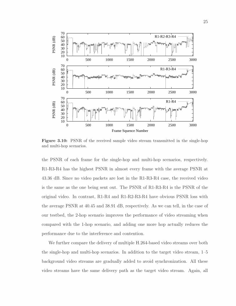
3.10 PSNR of the received sample video stream transmitted in the single-

hop and multi-hop scenarios. . . . . . . . . . . . . . . . . . . . . . . . 25

3.11 Average PSNR of the target video stream with multiple concurrent

video streams in the single-hop and multi-hop scenarios. . . . . . . . 26

4.1 The two-dimensional discrete time Markov chain with unsaturated

traffic, retry limit and post backoff stage in non-ideal channel condition. 30

5.1 Throughput vs. offered load by calculation and simulation. . . . . . . 46

5.2 The maximum achieved throughput with increased source-destination

separations. . . . . . . . . . . . . . . . . . . . . . . . . . . . . . . . . 47

ix

5.3 The PLRI of the first video stream with multiple concurrent video

streams in the single-hop and multi-hop scenarios. . . . . . . . . . . . 50

5.4 The average PSNR of the first video stream with multiple concurrent

video streams in the single-hop and multi-hop scenarios. . . . . . . . 52

5.5 The average frame delay of the first video stream with multiple con-

current video streams in the single-hop and multi-hop scenarios. . . . 53

5.6 The maximum accumulated frame jitter of the first video stream with

multiple video streams in the single-hop and multi-hop scenarios. . . 54

5.7 A general topology for 2-hop scenario. Two video clients (D1 and D2)

are x meters away from each other and 18 meters away from the source

router (S). The relay router (R) is at the center of the triangle (D1,

S, D2). . . . . . . . . . . . . . . . . . . . . . . . . . . . . . . . . . . 55

5.8 Average PSNR in the 2-hop scenario with the increased distance (x)

between the two video clients (D1 and D2). . . . . . . . . . . . . . . 56

6.1 Video streaming data rate: without rate control, with GOP-based rate

control, and with MW-based rate control (window size: 12 frames). . 61

6.2 The PLRI of the first video stream with multiple video streams.

(GOP-base smoothing vs. without smoothing) . . . . . . . . . . . . . 62

6.3 The average PSNR of the first video stream in multiple video streams.

(GOP-base smoothing vs. without smoothing) . . . . . . . . . . . . . 63

6.4 The PLRI of the first video stream with multiple video streams: 2

streams (1-hop), 5 streams (2-hop) and 4 streams (3-hop). The inter-

face queue buffer size increases from 192 KB to 1536 KB. . . . . . . . 66

6.5 The average frame delay of the first video stream with multiple video

streams: 2 streams (1-hop), 5 streams (2-hop) and 4 streams (3-hop).

The interface queue buffer size increases from 192 KB to 1536 KB. . . 67

x

List of Symbols

τ Per station transmission probability in a generic time slot

p Equivalent packet transmission failure probability

pc Packet collision probability

pe Transmission error probability

(i, k) Backoff counter state

Wi Contention window size

r Maximum backoff stage

q Probability of at least one packet awaiting in transmission queue

after a packet is sent out or dropped

Pi Probability of the channel is sensed idle in the post backoff stage

Tc Average channel time spent when a packet collision occurs

Ts Average channel time of a successful transmission

Te Average channel time spent when a packet transmission error occurs

S System throughput

xi

Acknowledgements

I wish to acknowledge the individuals who have helped guide my research during

the last one year. I recognize my wonderful supervisor, Dr. Jianping Pan, for his end-

less support, valuable guidance and encouragement throughout my whole graduate

study.

I wish to thank my thesis committee members: Dr. Sudhakar Ganti and Dr. Man-

tis Cheng for their valuable suggestions and encouragement.

Lastly, I wish to thank my family and friends. Without them, I would never go

this far.

xii

To my dear wife, Julia

1

Chapter 1

Introduction

Internet Protocol Television (IPTV) has attracted a lot of attention recently from

both academia and industry. It is believed that IPTV is going to be the next “killer”

application on the Internet in the near future. Internet service providers have high

expections on the large revenue that IPTV services can potentially generate. In fact,

many service providers are competing with time and each other to upgrade their

backbone and access networks, and sign up early subscribers [1].

As one of its attractive features, IPTV allows high definition television (HDTV)

programs to be delivered through the broadband access networks to the subscribers’

doorsteps. New high-speed communication technologies such as Wavelength Division

Multiplexing (WDM), Digital Subscriber Line (DSL), Hybrid Fiber-Coaxial (HFC)

and Fiber-To-The-Premise (FTTP), make the core and access networks no longer the

bottleneck of the end-to-end IPTV service delivery. Meanwhile, distributing IPTV

signals to each room in a house imposes a new challenge, since most current home

networks cannot meet the stringent quality-of-service (QoS) requirements of high-

quality video streaming in IPTV services [1].

As one of the traditional solutions, Ethernet is the currently preferred technology

for IPTV in-home distribution. Many commercial buildings and new houses are

Ethernet ready through Structured Wiring. However, for the vast majority of the

2

existing houses, Structured Wiring is not available. Rewiring costs turn out to be

prohibitively expensive and running Ethernet cable along hallway corners or even

outside the building could be awkward. There are several industry groups prompting

“no-new-wires” technologies to transport data and video over the existing household

cableline, phoneline and powerline plants [2]. However, the achievable performance

and availability of these technologies still need to be determined. Therefore, wireless

technologies, particularly IEEE 802.11-based ones, become the first choice by many

consumers for home networks.

IEEE 802.11 wireless local area network (WLAN) [3] has been adopted pervasively

in home networks due to its flexibility and affordability. The current main-stream

wireless home routers have embedded wireless Access Points (APs) supporting one

or several modes of IEEE 802.11a/b/g. Most portable computers come with wireless

hardware by default. People are becoming accustomed to turning on their laptop

computers and connecting to the wireless networks at home/work. Likely, IEEE

802.11 WLAN will be the preferred home network technology for IPTV services if it

can meet the service requirements of high-quality video streaming.

A common IEEE 802.11 wireless home network consists of a single wireless router

and multiple clients, the so-called single-hop wireless network. The router connects

to the service provider’s network by cable, and relays the data traffic to the clients

through wireless links. Ideally, IEEE 802.11b can support data rate up to 11 Mbps

and 802.11a/g up to 54 Mbps, which appears to be sufficient for IPTV services. How-

ever, the performance and coverage of a single-hop wireless network are significantly

affected by environmental factors. On the path from the transmitter to the receiver,

wireless signals are heavily attenuated and reflected by floors, walls, furniture and

moving objects such as people and pets. Therefore, the coverage of single-hop WLANs

in reality is more limited than in an ideal environment. Our experiment results show

that a single wireless router can only support high data rate in a limited range, which

3

is not sufficient to cover a typical house in North America. In addition, IEEE 802.11

devices are interfered by cordless phones, microwaves and other appliances working in

the same unlicensed frequency bands. Due to those uncertainties, thus far consumers

and service providers have rarely adopted WLAN for IPTV in-home distribution.

Two major approaches have been adopted to address the coverage issue. The first

approach is to increase the transmission power (TxPower) of the AP. However, when

the TxPower level is above a certain threshold, the noise level increases faster than the

received signal level does. As a result, further increasing the TxPower deteriorates the

received Signal-to-Noise Ratio (SNR) and diminishes the coverage. Moreover, a high

TxPower causes more interference to neighbours’ wireless devices and brings potential

wireless security problems as well. The second approach is to use multi-hop wireless

networks. In IEEE 802.11 WLANs, a common multi-hop wireless implementation is

the “Wireless Distribution System” (WDS). It interconnects multiple APs wirelessly

to relay IEEE 802.11 MAC frames. The performance of multi-hop wireless networks

is still not well studied in real environment. It is commonly believed that multi-hop

wireless networks trade off the achievable throughput to increasing the coverage, since

adding more relays in the same wireless channel increases the link contention.

Through the measurement on a multi-hop wireless testbed, we have found that

in contrast to the common belief, the tradeoff between coverage and capacity is far

from trivial. Modern wireless communication technologies such as IEEE 802.11g

usually support multiple transmission data rates (TxRate). When adding a relay,

link contention will increase, but links may be able to transmit at a higher TxRate

because the received signal quality is improved at the same time. The balance between

the increased contention and the increased TxRate is subtle. Therefore, it is possible

to improve both coverage and throughput at the same time for certain scenarios.

In this research, we first identified the needs for multi-hop wireless networks in

IPTV in-home distribution through experimentation on a multi-hop wireless testbed.

4

To emulate the multi-hop wireless networks in a household environment, we have built

an IEEE 802.11g WDS-based multi-hop wireless testbed. We evaluated the physical

and link layer performance as well as the performance of high-definition (HD) format

video streaming in different multi-hop scenarios. Through the experiment results,

we found that multi-hop wireless networks can increase the coverage and support

high-quality video streaming for IPTV services in a balanced manner.

Furthermore, to extend the research to generic scenarios, we used both perfor-

mance analysis and network simulation approaches to study the throughput and video

streaming performance of multi-hop wireless networks. We extended the discrete time

Markov chain model in [4] to analyze the throughput of IEEE 802.11 multi-hop wire-

less networks in both saturated and unsaturated traffic conditions. As an extension

to the existing models, our proposed model considers transmission errors, the post

backoff stage as well as the retry limits. It can better capture the characteristics

in a real household environment. From the throughput analysis, we ascertained the

guideline of how the multi-hop wireless networks should be deployed.

Afterwards, we built a model for network simulation. In the simulation, we

applied a Signal-Interference-to-Noise Ratio (SINR) based multi-rate extension [5]

to the Network Simulator version 2 (ns-2 ) [6] and integrated the simulator with

our video performance evaluation tool. Using this extended tool, we evaluated the

application-oriented performance metrics such as Peak Signal-to-Noise Ratio (PSNR)

and frame delay/jitter for video streaming over multiple hops and with multiple

streams. The simulation results further validate the measurement observation we

had on the testbed, and give an insight on the intrinsic tradeoff between coverage

and capacity. Our research also provides some guidance on how to achieve the optimal

balance for a given scenario.

The contributions of this thesis have three aspects. First, we built a multi-hop

wireless testbed based on existing technology to identify the research problem. It

5

shows that our research is practical and challenging. Second, our analytical model

and simulation model extend the existing work, and better capture the characteristics

of IEEE 802.11g wireless networks in a household environment with high attenuation

and interference. Our models are suitable for the research on video streaming over

wireless networks, especially for H.264-based HDTV in-home distribution over IEEE

802.11 WDS. Third, our analysis and simulation results reveal a wide spectrum of

the coverage-capacity tradoff and help identify how to achieve the best possible bal-

ance. We believe this work is of particular importance for service providers that are

deploying IPTV services.

The rest of the thesis is organized as follows. In Chapter 2, we review the cur-

rent state-of-the-art approaches in IPTV in-home distribution, and summarize the

related work on throughput analysis of IEEE 802.11 WLAN and video streaming

over wireless networks. In Chapter 3, we present our multi-hop wireless testbed and

video streaming experimentation. In Chapter 4, we present our analytical model and

the detailed throughput analysis method. In Chapter 5, we first validate our analyt-

ical and simulation models by calculation and ns-2 simulation, then we evaluate and

compare the performance of video streaming over single-hop and multi-hop wireless

scenarios in simulation. In Chapter 6, we discuss the ways to further improve video

streaming quality, followed by conclusions in Chapter 7.

6

Chapter 2

Background and Related Work

In this chapter, we first give the background of current IPTV in-home distribution

solutions and H.264-based video streaming. After that, we review the existing work

on performance analysis of IEEE 802.11 WLANs and video streaming over wireless

networks.

2.1 IPTV In-Home Distribution

With the advance of the telecommunication technologies in both backbone and access

networks, it is now possible to deliver IPTV services to the doorstep of subscribers.

How to deliver IPTV signals with stringent QoS requirements to one or more TV sets

throughout the house becomes a challenge for current home networks [1]. Ethernet

is the preferred LAN technology, but many existing houses need rewiring Ethernet

cables. Rewiring has been cited as one major barrier to a large-scale, profitable

IPTV market because of the high cost and inconvenience. Both customers and ser-

vice providers are looking at other alternatives such as “no-new-wires” and wireless

solutions.

2.1.1 No-new-wires Solutions

The so-called “no-new-wires” technologies, which reuse the existing household cable-

line, phoneline and powerline plants for high speed data communications, have been

7

prompted by several industry groups in the recent years [2]. The newest standards

such as MoCA 1.0 [7], HPNA 3.1 [8] and HPAV [9], all claim to support raw data rate

well above 100 Mbps, but several practical issues still remain. First, the availability

and achievable throughput of these technologies are quite limited in reality. Second,

even if there are “no-new-wires” outlets in a room, they may not be located within

a convenient distance to the TV set. Third, due to the broadcast and half-duplex

nature of these wires, spatial reuse is not possible throughout a house. Lastly, some

wire plants are actually shared by the entire neighborhood, which adds additional

security concerns. For these reasons, many consumers prefer wireless solutions for

the flexibility and mobility.

2.1.2 Wireless Solutions

So far, IEEE 802.11 b/g WLAN is the pervasive wireless solution and has been widely

deployed at home/offices. Other emerging high-speed wireless technologies such as

IEEE 802.11n can provide raw data rate up to 540 Mbps; Ultra-Wide-Band (UWB)

can go up to several hundred Mbps and even Gbps within 10 m [10]; Millimeter Wave

(mmWave) is expected to deliver 1–10 Gbps within a short line-of-sight range [11].

All these new technologies can support a high data rate within a short distance in

an ideal environment. However, the wireless channel condition in a typical household

environment is far from ideal. The signal quality is significantly impaired by obstacles,

fading and interference from other wireless devices. Single-hop wireless networks can

only provide limited coverage and throughput when compared with their theoretical

limits. Therefore, it is necessary to adopt multi-hop wireless networks to increase the

coverage without compromising the performance too much.

2.1.3 Multi-hop Wireless Solutions

For IEEE 802.11 WLAN, the popular multi-hop wireless implementation is the so-

called “Wireless Distribution System” (WDS). A WDS is a system that enables the

8

interconnection of APs wirelessly. WDS systems are implemented using the four-

address IEEE 802.11 frame format defined in [3]. So far, two major categories of

WDS, the static WDS and dynamic WDS, are available in the wireless home router

market. With the static WDS, the WDS links are manually configured on each AP

and recorded in an internal WDS link table. The relay AP uses the fourth address in

the MAC frame to find the path to the destination. Different from the static WDS,

the dynamic WDS allows an AP to automatically learn about other WDS-capable

APs in the vicinity. In our research, we only used the static WDS for its easiness of

controlling the traffic delivery path.

WDS is generally used to increase the coverage of an IEEE 802.11 LAN. It allows

a wireless station to associate with the AP of the best signal quality. For example, if

an AP is deployed on the ground floor to relay the traffic from the home gateway in

the basement, a wireless station on the second floor can associate with the relay AP

rather than the home gateway in the basement to get a better signal quality. However,

in order to provide seamless roaming and allow APs to reach each other wirelessly,

APs and stations in a WDS have to use the same wireless channel. This increases the

interference and media access contention due to the shared half-duplex nature of the

wireless media. It is commonly believed that although WDS can increase wireless

coverage, it only offers a fraction of bandwidth to wireless stations.

2.1.4 H.264-based Video Streaming

Recently, the H.264 standard has been adopted for HD format video streaming by

IPTV service providers for its high efficiency in video compression. H.264, also known

as MPEG-4 Part 10 Advanced Video Coding (AVC), is the newest video coding stan-

dard developed by the joint effort of ITU-T and ISO MPEG committee [12]. Its latest

achievement is the H.264 with Fidelity Range Extensions (FRExt) amendment [13].

With the advanced prediction, compression and encoding techniques, this newly de-

veloped H.264 standard typically achieves the same reproduction quality at half or

9

even less of the data rate required by the MPEG-2 encoders [14, 15]. For example, a

single MPEG-2 encoded HDTV channel has an average data rate of 12 Mbps. The

same channel encoded by the H.264 encoders only has an average data rate of 5–

6 Mbps. However, the data rate of the H.264 encoded video has significantly higher

peak-to-average ratio than that of either the MPEG-2 or MPEG-4 Part 2 encoded

ones [16].

The high traffic variation of H.264-based video stream introduces new challenges

for the IPTV in-home distribution networks as well. It is very difficult to allocate

network resources efficiently. Allocating at the average rate will cause excessive packet

delay and loss. Alternatively, allocating at the peak rate will greatly reduce the

number of video streams that can be supported. Furthermore, the high efficiency

coding makes the compressed video streams less tolerant to packet loss and delay.

The frame correlation makes packet loss and delay alone not sufficient to describe the

quality degradation because packet loss in key frames can affect multiple follow-on

frames.

In summary, the IPTV in-home distribution, especially the wireless solution, is

still a challenging problem. Conventional single-hop wireless networks are limited

by their coverage, and cannot provide IPTV support to an entire house. Multi-

hop wireless networks such as WDS networks, can increase the coverage but the

performance is still not well understood. Moreover, high efficiency video compression

standards such as H.264, can reduce the bandwidth requirement, but bring other

challenges for the in-home distribution networks as well. Therefore, we focus on

H.264-based video streaming over multi-hop wireless networks in this research.

10

2.2 Related Work

2.2.1 Throughput Analysis of Wireless Networks

The throughput of distributed coordination function (DCF) for IEEE 802.11 Media

Access Control (MAC) [3] has been extensively studied in the literature. We sum-

marize the most related existing work as follows. In his seminal paper [4], Bianchi

proposed a two-dimensional discrete time Markov chain model to analyze the satu-

rated throughput of DCF in ideal channels. This model relies on the assumption that

the packet collision probability is constant and independent of previous transmission

attempts. In order to simplify the analysis, this model assumes unlimited retries

and ignores the post backoff behaviour of IEEE 802.11 DCF. Malone et al. extended

Bianchi’s model to the case of unsaturated traffic conditions in [17]. This model takes

the post backoff behaviour into consideration. However, the authors assumed an ideal

channel condition and unlimited retries as well. In [18], Daneshgaran et al. proposed

another extended model to consider the non-ideal channel condition and unsaturated

traffic. The authors assumed that the transmission error and packet collisions are

independent, so they used an equivalent probability of failed transmission to replace

the collision probability p in Bianchi’s model. The post backoff stage is simplified

with a single idle state and unlimited retries are assumed as well.

All the above approaches have some simplifications when modeling the IEEE

802.11 DCF, so they are not realistic enough to capture the characteristics of IPTV

in-home distribution. First, wireless networks in a household environment do not

have ideal channel conditions. They are subject to channel errors caused by many

environmental factors. Second, wireless home networks usually work in unsaturated

mode since the number of wireless nodes in a house is typically limited. Third, the

retry limit parameter and the post backoff behaviour in DCF have impacts on the

throughput, packet delay and jitter. It is necessary to take the retry limit and the

11

post backoff process into consideration. For these reasons, we propose an extended

Markov model to study the throughput in non-ideal channels with unsaturated traffic

conditions. Both the retry limit and the post backoff behaviour are taken into account

in the model.

Other related work extended Bianchi’s model to capture the QoS enhancement

features proposed in IEEE 802.11e standard [19]. In [20], the authors used multiple

queues with different contention characteristics in IEEE 802.11e with QoS provision-

ing. In [21], the authors proposed a Markov chain model for the Enhanced Distributed

Channel Access (EDCA) in IEEE 802.11e. New features, such as virtual collision,

arbitration interframe spaces (AIFS), and different contention windows for virtual

queues, are taken into account. The authors also presented methods to analyze the

average packet delay and the throughput of the traffic with differentiated services.

However, both these models assumed an ideal channel condition.

2.2.2 Video Streaming Over Wireless Networks

Video streaming over wireless networks has received intensive attention in recent

years. Here, we list the most relevant work. On the performance evaluation side,

[22,23] focused on video streaming over existing IEEE 802.11 wireless networks with

different encoding schemes, background traffic, packet size and so on, and proposed

the optimal encoding and MAC layer parameters for certain scenarios. On the per-

formance improvement side, [24] used application-level approaches to deal with high

packet loss and delay variation in wireless networks, such as retransmission and For-

ward Error Control (FEC). In [25], the authors proposed cross-layer architecture

approaches to map application-level video characteristics such as frame types, to net-

work and MAC layer parameters such as TxRate, retry limit, and so on, as well as

IEEE 802.11e priorities. However, most existing work focuses on single-hop scenarios

using IEEE 802.11b. For HD format IPTV in-home distribution, the coverage and

throughput of a single wireless router is quite limited. To deliver multiple high-quality

12

video streams across a house, it is advantageous to use multi-hop IEEE 802.11g net-

works with higher and more flexible TxRate.

Compared with the existing work, our research is different in three aspects.

Firstly, our research scenario targeted multi-hop IEEE 802.11 WLAN instead of the

single-hop wireless scenario adopted in the articles referenced. Secondly, most ex-

isting work only employed IEEE 802.11b based simulation, whereas we adopt both

experimentation and simulation approaches in IEEE 802.11g mode. IEEE 802.11g

standard supports higher raw rates than IEEE 802.11b and uses different modulation

schemes, which have very different characteristics [26, 27]. Thirdly, we evaluated the

performance of H.264-based video streaming at the application level as well as the

packet level. For these reasons, our research is more realistic and up-to-date.

13

Chapter 3

Video Streaming over Multi-hop Wireless

Testbed Experimentation

As discussed in Chapter 1 and Chapter 2, delivering video packets with stringent QoS

requirements over IEEE 802.11 wireless networks is very challenging. In a household

environment, the link quality drops quickly when the distance between the transmit-

ter and the receiver increases due to the high attenuation and interference. Since

IEEE 802.11 b/g devices support multiple TxRate modes for different link qualities,

the single-hop wireless link can work at a low TxRate mode when the received signal

quality is poor. By adding a relay, the multi-hop wireless link reduces the distance

between the transmitter and the receiver, so the received signal quality is improved,

and the wireless nodes can work at a high TxRate. Although the multi-hop link

has more link contention, it can achieve a better performance than the single-hop

link because of the higher TxRate in certain scenarios. Motivated by this idea, we

built a WDS-based multi-hop wireless testbed to emulate a typical wireless home

network. Through the evaluation of both the link layer performance and the video

streaming performance, we discovered that it is possible to increase the coverage and

performance at the same time, which allows the high-quality video streaming to be

delivered in multiple hops across the house.

14

R1R4 R2

R3

Figure 3.1: The location of the routers in the multi-hop wireless testbed.

In the rest of this chapter, we first present our multi-hop wireless testbed and

video streaming evaluation framework in Section 3.1. We then show the channel

characteristics of our testing environment and the link performance in Section 3.2.

Finally, we evaluate the video streaming performance in the 1-hop, 2-hop and 3-hop

scenarios in Section 3.3.

3.1 Multi-hop Wireless Testbed

3.1.1 Testbed Configuration

Our multimedia over multi-hop wireless testbed is built with a popular type of IEEE

802.11g wireless home router, Linksys WRT54GL. This router has a 200 MHz MIPS

CPU, 16 MB RAM and 4 MB flash memory as storage. We installed a Linux-

compatible open source firmware, OpenWrt [28], in the router. This firmware provides

WDS support and many advanced control capabilities. The router has a Broadcom-

based wireless chipset, and its device driver can set the wireless TxPower within a

certain range and can choose a particular TxRate as well.

Figure 3.1 shows the location of the four wireless routers (R1, R2, R3 and R4)

in our testbed. The routers are deployed in a linear topology with exponentially

increased spacing. R1 and R2 are in the same room without obstacles. R2 and R3

are separated by three walls, while R3 and R4 have a doubled distance with the same

number of walls in between. We use R1 as the video source and R4 as the video

destination, and the overall distance between them is about 33 m. Each router is at

a location least affected by uncontrollable factors such as moving objects.

15

Figure 3.2: The link topology of the multi-hop wireless testbed.

Figure 3.2 shows the link topology of the testbed. For the wireless links, we employ

the static WDS configuration and static routing scheme on the source and relay

routers (R1, R2 and R3) to control the delivery path of the packets. By enabling the

radio of R2 and R3 and by changing WDS link table and static routes accordingly, we

are able to create the 1-hop, 2-hop and 3-hop scenarios. To minimize the interference

from other wireless devices, we choose an unused non-overlapping radio channel in

our building. As show in the figure, each router in the testbed has a direct Fast

Ethernet link connected to an Ethernet switch for control purpose. Since the achieved

throughput of the Ethernet links is much more than that of the wireless links and

the packet delay of the Ethernet links is low and stable, these control links will not

become the bottleneck in the testbed. Moreover, the video streaming server and

client computers are connected to R1 and R4 respectively through Fast Ethernet

links. For the same reason, the Ethernet links are not the bottleneck either.

16

3.1.2 Video Evaluation Framework

For video streaming evaluation, we use a video performance evaluation tool, Evalvid [29]

in our experiment. This tool provides a set of programs for analyzing video trace files

and calculating the video performance metrics including packet loss ratio, frame delay

and jitter, and frame PSNR. As an objective video quality metric, PSNR estimates

the quality of a reconstructed frame compared with an original frame. Reconstructed

frames with higher PSNRs are perceived better. Typical PSNR values range between

20 and 40 dB. Generally, when the PSNR difference of the same picture in two videos

is more than 0.5 dB, the perceptual difference would be visible [30]. Subjective video

quality metrics such as the Mean Opinion Score (MOS) can be obtained from the

PSNR as well. It has been cited that the MOS is correlated to the average PSNR.

When the average PSNR is greater than 37 dB, the MOS is 5 (excellent) [31]. From

our video evaluation results, we have found that the received video is judged as good

quality (MOS ≥ 4) when the average PSNR is greater than 36 dB. Therefore, in

the thesis, we use the average PSNR of 36 dB as the threshold for acceptable video

quality.

The process of evaluating a specific video is as follows. We first encode the raw

video source in H.264 format. Next, the H.264 video is hinted and sent from the source

to the destination through the target network. At the mean time, two tcpdump [32]

processes are started at both the source and destination sides to capture the sending

and receiving events of the video packets. These events are recorded in the trace file

with a unique sequence number and a timestamp. Besides the video packet traces,

the video frame trace, including the frame type and frame size, are also recorded at

the source. After the video stream is finished, the Evalvid analyzes the three trace

files, and then obtains the packet loss ratio, frame delay and jitter. Furthermore, the

evaluation program reconstructs the received video by removing the video content

in the lost packets from the original video. Finally, the received H.264-based video

17

0

0.02

0.04

0.06

0.08

0.1

0.12

0.14

0.16

0 500 1000 1500 2000 2500 3000

Fra

me

Siz

e (M

B)

Frame Sequence Number

0

0.02

0.04

0.06

0.08

0.1

0.12

0.14

0.16

0 500 1000 1500 2000 2500 3000

Fra

me

Siz

e (M

B)

Frame Sequence Number

Figure 3.3: Frame size of the sample video stream.

is decoded and Evalvid compares the received video and the original video frame by

frame, and then calculates the frame PSNR.

In our experiment and simulation, we use a two-minute SONY HD camera demo

video clip as the sample video source. It has 1,280 x 720 pixels resolution at 24

frame per second. The video is encoded by the H.264 reference encoder [33]. The

average data rate and peak data rate of the video stream traffic are around 2.0 Mbps

and 32.0 Mbps, respectively. Generally, H.264-based videos are patterned as a group

of pictures (GOP). Each GOP has a fixed structure, including one I-frame, several

P-frames and a certain number of B-frames between I and P-frames. The GOP

structure of our sample video is “IBBPBBPBBPBB.” Table 3.1 lists the important

characteristics of this video stream. The video frame size is shown in Figure 3.3.

18

Table 3.1: Statistics of the sample video

Parameter Value

Picture resolution 1,280 x 720 pixelsFrame refresh rate 24 frame/secTotal frames 3,016Number of I-frames 252Number of P-frames 754Number of B-frames 2,010Avg. I-frame size 31,992 bytesAvg. P-frame size 23,463 bytesAvg. B-frame size 2,623 bytesGOP size 12 framesGOP structure IBBPBBPBBPBBTotal packets 22,848

3.2 Wireless Link Characterization

3.2.1 Channel Characterization

First, we evaluate the received SNR between all four routers. We read the received

signal power level and noise level (in dBm) measured by the wireless chip directly

from the device driver. The received SNR in dB can be obtained by subtracting the

noise level from the received signal power level. In order to eliminate the potential

interference from other wireless devices, our measurement was conducted in late

nights when few people were using the wireless devices. In this way, the measurement

provides the basic condition of the wireless links in our testbed.

As shown in Figure 3.4, at a given TxPower, the received SNR decreases with

the increased distance between the transmitter and receiver as well as the number of

walls due to signal attenuation. On average, the SNR of R1-R3 is about 10 dB lower

than that of R1-R2, and is about 20 dB higher than that of R1-R4, which indicates

a high attenuation level by walls.

In general, the received SNR increases with the increased TxPower, although the

19

0

5

10

15

20

25

30

35

40

45

50

55

8 10 12 14 16 18 20

SNR

(dB

)

TxPower (dBm)

R1-R2R1-R3R1-R4R2-R3R3-R4

Figure 3.4: Average received SNR with different TxPower.

growth rate varies for different links. For R1-R2, which are in the same room and

have no obstacles in-between, there is an optimal TxPower level around 18 dBm,

where the received SNR is maximized. 18 dBm actually is the recommended power

setting for this router and is the default value in many wireless home router firmwares.

Further increasing TxPower raises the noise level for R1-R2 as well and results the

decrease of received SNR, although increased TxPower does increase the SNR for

other router pairs. For the results in the next section, we use the default 18 dBm

TxPower setting for all routers.

3.2.2 Link Layer Performance

Next, we measure the link properties such as loss and delay for the single-hop link (R1-

R4) and multi-hop links (R1-R3-R4 and R1-R2-R3-R4). A probe packet of 64 bytes,

the minimal Ethernet frame size, is sent from R1, potentially going through R2 and

R3 for multi-hop links, and echoed by R4. The echo packet returns to R1 through the

20

0

20

40

60

80

100

1 2 5.5 6 9 11 12 18 24 36 48 54

Pack

et L

oss

Rat

io (

%)

TxRate (Mbps)

R1-R2R1-R3R1-R4

Figure 3.5: Packet loss ratio over single-hop links.

control link. Packets are sequenced and timestamped, so packet loss ratio (PLR) and

round-trip time (RTT) can be calculated. PLR and RTT are good indicators of link

loss and delay, respectively. Moreover, since the return link (switched Fast Ethernet)

is very stable and has no extra traffic, the one-way delay (OWD) of the wireless links

can be obtained by subtracting the average packet delay of the control links from the

RTT that we measured. In order to establish a baseline, MAC retransmission is not

used (unless otherwise stated) and there is no MAC contention introduced by this

single over-the-air packet in this test. The results shown below are averaged from 20

runs of tests, each of which has 100 probe packets.

As shown in Figure 3.5, the PLR increases while the TxRate increases in general.

This is because that at a given SNR, a higher TxRate implies a higher bit error rate

(BER), which results more packet loss. R1-R2 and R1-R3 have similar link loss, since

the SNR of both links are sufficiently high to support even 54 Mbps. For R1-R4, due

to a low SNR shown in Figure 3.4, it suffers a high PLR (> 30%). Moreover, all

21

0

20

40

60

80

100

1 2 5.5 6 9 11 12 18 24 36 48 54

Pack

et L

oss

Rat

io (

%)

TxRate (Mbps)

R1-R2-R3-R4R1-R3-R4

R1-R4R1-R4 (w/ retry)

Figure 3.6: Packet loss ratio over multi-hop links.

IEEE 802.11g mode TxRates (6, 9, 12, 18, 24, 36, 48, and 54 Mbps) using OFDM

modulation suffer a much higher PLR than all IEEE 802.11b mode TxRates (1, 2,

5.5, and 11 Mbps) using CCK modulation, since the SNR for each OFDM sub-carrier

is very low in this case.

As shown in Figure 3.6, the multi-hop links (R1-R3-R4 and R1-R2-R3-R4) have

much lower PLR than that of the single-hop link (R1-R4) for all TxRates since the

received SNR at each hop is sufficiently high. For comparison, the PLR of R1-R3-R4

is higher than that of R1-R3 and R3-R4 individually, since its packets travel over the

air twice, but is lower than the sum of that of R1-R3 and R3-R4. We also measure

the scenario for all links with MAC retransmission: the PLR for all multi-hop links

is 0, and that for R1-R4 with retry is still quite high.

For link delay, in this test it only includes transmission, propagation and process-

ing delay, since there is no MAC contention and queuing delay involved. As shown in

Figure 3.7, normally, longer links have higher propagation delay, and higher TxRate

22

0

0.5

1

1.5

2

2.5

3

3.5

4

1 2 5.5 6 9 11 12 18 24 36 48 54

Del

ay (

ms)

TxRate (Mbps)

R1-R2R1-R3R1-R4

Figure 3.7: One-way packet delay over single-hop links.

0

0.5

1

1.5

2

2.5

3

3.5

4

1 2 5.5 6 9 11 12 18 24 36 48 54

Del

ay (

ms)

TxRate (Mbps)

R1-R2-R3-R4R1-R3-R4

R1-R4R1-R4 (w/ retry)

Figure 3.8: One-way packet delay over multi-hop links.

23

leads to lower transmission delay for packets of the same size. Nevertheless, when the

SNR is sufficiently high for R1-R2 and R1-R3, OFDM is efficient with low processing

delay at 6 and 9 Mbps. The resultant delay is even lower than that at 11 Mbps with

CCK modulation. The delay of multi-hop links is shown in Figure 3.8. In general, the

multi-hop links, as their packets go over the air more than once, have longer link delay

than the single-hop links do. Due to the low SNR in each sub-carrier, R1-R4 suffers

high processing delay with OFDM modulation. But when the SNR is sufficiently

high for R1-R3-R4 and R1-R2-R3-R4, OFDM is efficient with low processing delay

at 6 and 9 Mbps, and the resultant delay is even lower than that at 11 Mbps with

CCK modulation. R1-R3 and R3-R4 show similar behaviors. When MAC retrans-

mission is enabled for R1-R4, the delay is increased greatly due to multiple attempts

of retransmission.

Through Figure 3.6 and Figure 3.8, we have found that R1-R2-R3-R4 does not

further reduce link loss when compared with R1-R3-R4, but it does increase delay

considerably. This suggests whether to add an extra relay router should be balanced

between the packet loss to be reduced and the delay to be increased.

3.3 Video Streaming Performance Evaluation

3.3.1 Methodology

We then evaluate the application properties, such as frame loss and PSNR, for H.264-

based video streaming over the multi-hop wireless scenarios. The sample video

streams are sent out from the video server to R1, then potentially go through R2

and R3 for multi-hop scenarios, arrive at R4 and are finally forwarded to the video

client through the Fast Ethernet link. By using the video evaluation methodology

introduced in Section 3.1.2, we obtain the frame loss ratio (FLR), frame delay/jitter,

and frame PSNR. In this test, we set the MAC retry limit to 7, the default value

of the firmware. MAC contention is possible in this test since multiple transmitters

24

0

10

20

30

40

50

60

70

80

90

100

2 5.5 6 9 11 12 18 24 36 48 54

Fram

e L

ose

Rat

io (

%)

TxRate (Mbps)

R1-R2-R3-R4R1-R3-R4

R1-R4

Figure 3.9: The frame loss ratio of a single video stream in the single-hop and multi-hopscenarios.

may compete for the shared channel.

3.3.2 Performance Evaluation

As shown in Figure 3.9, R1-R4 has a higher FLR when the TxRate is above 12 Mbps

due to the lower SNR, but it has an FLR lower than that of either R1-R2-R3-R4 or

R1-R3-R4 when TxRate is below 11 Mbps. This is because that TxRate has been

fixed in this test and multi-hop links sharing the same channel have severe contention

when the TxRate is low and packet air time is long. When TxRate increases, packet

air time reduces and link contention becomes less obvious, which leads to a lower FLR

for multi-hop scenarios. In fact, multi-hop scenarios can sustain higher TxRates due

to the higher SNR.

We further compare the received video quality of the single-hop scenario and that

of the multi-hop scenarios. In order to show the best case of each scenario, we set auto

TxRate for all routers to make them work at the optimal mode. Figure 3.10 shows

25

10 20 30 40 50 60 70

0 500 1000 1500 2000 2500 3000

PSN

R (

dB) R1-R2-R3-R4

10 20 30 40 50 60 70

0 500 1000 1500 2000 2500 3000

PSN

R (

dB) R1-R3-R4

10 20 30 40 50 60 70

0 500 1000 1500 2000 2500 3000

PSN

R (

dB)

Frame Squence Number

R1-R4

Figure 3.10: PSNR of the received sample video stream transmitted in the single-hopand multi-hop scenarios.

the PSNR of each frame for the single-hop and multi-hop scenarios, respectively.

R1-R3-R4 has the highest PSNR in almost every frame with the average PSNR at

43.36 dB. Since no video packets are lost in the R1-R3-R4 case, the received video

is the same as the one being sent out. The PSNR of R1-R3-R4 is the PSNR of the

original video. In contrast, R1-R4 and R1-R2-R3-R4 have obvious PSNR loss with

the average PSNR at 40.45 and 38.91 dB, respectively. As we can tell, in the case of

our testbed, the 2-hop scenario improves the performance of video streaming when

compared with the 1-hop scenario, and adding one more hop actually reduces the

performance due to the interference and contention.

We further compare the delivery of multiple H.264-based video streams over both

the single-hop and multi-hop scenarios. In addition to the target video stream, 1–5

background video streams are gradually added to avoid synchronization. All these

video streams have the same delivery path as the target video stream. Again, all

26

10

15

20

25

30

35

40

45

50

1 2 3 4 5 6

Ave

rage

PSN

R (

dB)

Number of Video Streams

R1-R2-R3-R4R1-R3-R4

R1-R4

Figure 3.11: Average PSNR of the target video stream with multiple concurrent videostreams in the single-hop and multi-hop scenarios.

routers employ MAC retransmission and auto TxRate to adapt to wireless channel

condition in this test.

Figure 3.11 shows the average PSNR of the target video stream with different num-

ber of concurrent video streams for R1-R4, R1-R3-R4 and R1-R2-R3-R4. All three

scenarios have quality degradation when the number of streams increases. However,

the 2-hop scenario can support more video streams at higher PSNR than both the

1-hop and 3-hop scenario. The 1-hop scenario has the lowest PSNR due to the fact

of low SNR and the existence of background traffic. The 3-hop scenario initially can

maintain an acceptable PSNR, but drops very quickly when there are more than three

streams. Only the 2-hop scenario can support up to five streams with little quality

degradation, but its PSNR decreases when the number of stream is more than four.

27

3.4 Summary

In this chapter, we have presented our IEEE 802.11 WDS-based multi-hop wireless

testbed, which emulates a typical in-door environment. Through the wireless channel

and link performance measurements, we have identified that the traditional single-

hop infrastructure mode IEEE 802.11g WLANs can only provide limited capacity

and coverage in an in-door environment due to the high signal attenuation. In con-

trast, the multi-hop wireless networks increase both the coverage and capacity since

the multi-hop links greatly improve the received signal quality and work at high

TxRates. However, the excessively increased link contention will reduce the achiev-

able throughput. Further, we have evaluated the performance of H.264-based video

streaming over the 1-hop, 2-hop and 3-hop scenarios. Our experiment results reveal

that the multi-hop wireless network can provide better quality in video streaming

services than the single-hop one in a typical in-door environment, but the SNR im-

provement and link contention should be balanced. Admittedly, the experimentation

on the specific testbed is only a case study. Later, we use analytical model and

network simulation to study this problem in general scenarios.

28

Chapter 4

Throughput Analysis of Multi-hop

Wireless Networks

From the testbed experiments, we have found that the performance of video streaming

highly correlates to the achievable throughput. In this section, we first present a

two-dimensional discrete time Markov chain to model the behaviour of IEEE 802.11

backoff counter. After that, we use this model to evaluate the throughput of multi-

hop wireless networks.

Our throughput analysis only focuses on the IEEE 802.11 networks with the DCF

MAC access method. This is because most IEEE 802.11 networks in reality operate

in DCF mode. In addition, the other two MAC access methods—point coordination

function (PCF) and hybrid coordination function (HCF), are not well supported by

the majority of vendors due to the complexity and performance issues.

Our model extends the work proposed in [4] and [17] in three aspects. First, our

model focuses on unsaturated traffic condition in non-ideal channels. Second, it takes

the retry limit into consideration. Finally, it models the post backoff behaviour of

IEEE 802.11 DCF. Compared to the models in [4] and [17], this model is more realistic

to capture the characteristics of video streaming over IEEE 802.11g networks.

The rest of this chapter is is structured as follows. First, we present our proposed

29

model and then derive the variables of our interests. Finally, we show how to analyze

the saturated and unsaturated throughput of a multi-hop wireless network.

4.1 The Markov Chain Model

We hold the same fundamental assumption as in [4] that packets collide at each

transmission attempt with a constant and independent probability pc. We also as-

sume that the transmission errors caused by channel impairments are independent of

packet collisions. To simplify the analysis in this study, we assume that all packets

have the same size and the transmission error probability is a constant denoted by

pe. It is intuitive that transmission errors are independent of packet collisions. We

define an equivalent transmission failure probability p as follows.

p = 1 − (1 − pe)(1 − pc) = pc + pe − pcpe (4.1)

Following the approach in [4], we model the value of the backoff counter of a

wireless node by two stochastic processes denoted by (i, k). Process i is the backoff

stage from [0, r] where r is the maximum backoff stage. Process k is the value of the

current backoff counter ranged from [0, Wi − 1]. Wi is the Contention Window (CW)

size at backoff stage i. The state transition process is shown in Figure 4.1.

First, we present the state transition for the backoff stages from 0 to r − 1.

As shown in Figure 4.1, a node at backoff stage i freezes its backoff counter when

the medium is sensed busy. When the medium is idle, the node decrements the

counter by 1 in a fixed time slot. When the counter value reaches 0, the node will

attempt to transmit a packet. If the transmission fails with probability p due to either

transmission error or packet collision, the backoff counter state will move to stage

i+1 and a random backoff counter value will be uniformly chosen from [0, Wi+1 − 1].

If the transmission succeeds, the state will return to stage 0 with probability q. q is

the probability that there is at least one packet awaiting in the transmission queue

30

−1,W0−1−1,W0−2qPip

qPi(1−p)

(1−p)(1−q)

(1−p)(1−q)

1−q 1−q 1−q

(1−p)(1−q)

1−q

(1−p)(1−q)

1−q

q

q qq

1 1 1 1

1 1 1

1 1 1

p

p

p

p

0, W − 20 00, W −1

1

i, W −4i1 1

1 1111

1 1 1 1 1

1 11, W −3 1, W −2 1, W−1

i i, W −2ii, W −3 i, W −1i

m, W −5m m, W −4m m, W −3m m, W −2m m, W −1m

r, W −1rr, W −2rr,W −3rr, W −4rr, W −5rr, 0 r, 1

m, 1m, 0

1

1

1

i, 1

1, 11, 0

i, 0

0, 10, 0

−1, 1−1, 0

(1−p)q

(1−p)q

(1−p)q

(1−p)q

iq(1−P )

Figure 4.1: The two-dimensional discrete time Markov chain with unsaturated traffic,retry limit and post backoff stage in non-ideal channel condition.

of the node. The state transition probabilities are given as follows.

P [(i, k − 1)|(i, k)] = 1 0 < i ≤ r, 0 < k ≤ Wi − 1

P [(0, k)|(i, 0)] = (1−p)qWo

0 ≤ i < r, 0 ≤ k ≤ W0 − 1

P [(i, k)|(i − 1, 0)] = p

Wi

0 < i ≤ r, 0 ≤ k ≤ Wi − 1

Next, we show the state transition in the post backoff stage. The node starts a

backoff process immediately after a successful transmission even when its transmission

queue is empty. This behaviour is called post backoff. We use (−1, ∗) to denote the

post backoff states. A random value is chosen uniformly from [0,W0 − 1] for the

backoff counter when a post backoff process starts. During the period while the

backoff counter decrements to 0, if a packet arrives with probability q, the node will

move to the backoff stage 0 and inherit the current value of the backoff counter for the

regular backoff process. If the value of the counter is already 0 when a packet arrives

31

and the medium is idle, the node will transmit the packet immediately. In unsaturated

traffic condition, there is not always a packet awaiting in the transmission queue. The

post backoff behaviour reduces the packet delay and increases the throughput. The

related state transition probabilities are given as follows.

P [(−1, k − 1)|(−1, k)] = 1 − q 0 < k ≤ W0 − 1

P [(0, k − 1)|(−1, k)] = q 0 < k ≤ W0 − 1

P [(−1, k)|(i, 0)] = (1−p)(1−q)W0

0 ≤ i < r, 0 ≤ k ≤ W0 − 1

P [(−1, 0)|(−1, 0)] = 1 − q + qPi(1−p)W0

P [(−1, k)|(−1, 0)] = qPi(1−p)W0

0 < k ≤ W0 − 1

P [(1, k)|(−1, 0)] = qpPi

W1

0 ≤ k ≤ W1 − 1

P [(0, k)|(−1, 0)] = q(1−Pi)W0

0 ≤ k ≤ W0 − 1

Now, we show how the retry limit is incorporated in the backoff counter state

transition. In IEEE 802.11 standard, the station maintains a retry counter to record

the number of retransmissions that a packet has experienced. When the retry counter

reaches the retry limit, the station will drop the current packet to avoid excessive

delay for the other packets in the transmission queue. The node resets the retry

counter when it starts to transmit a new packet. We define the maximum backoff

stage r as the last backoff stage before the retry counter reaches the limit. When the

backoff counter state is (r, 0), it moves to (−1, ∗) with probability 1 − q if no packet

is in the transmission queue; otherwise, the state moves to (0, ∗). The related state

transition probabilities are given as follows.

P [(−1, k)|(r, 0)] = 1−q

W0

0 ≤ k ≤ W0 − 1

P [(0, k)|(r, 0)] = q

W0

0 ≤ k ≤ W0 − 1

32

Notice that there are two different cases when the retry limit is considered in

the model. The maximum backoff stage r is determined by the retry limit but the

maximum contention window Wm is determined by the IEEE 802.11 MAC parameter

CWmax. The contention window increases exponentially when the backoff stage is

less than m. When the contention window reaches Wm, it will not increase anymore.

Therefore, we have the following relations:

Wi =

2iW0 i ≤ m

2mW0 i > m

In order to analyze the throughput, we need to know τ , the per station trans-

mission probability in a generic time slot. Here, we show the derivation process of

obtaining τ . The steady state probability of the backoff counter state is denoted by

b(i, k).

First, we deal with the b(−1, ∗) chain. Notice that all b(i, 0) when i ≥ 1 have the

following recursive relation:

b(i, 0) = pb(i − 1, 0) = pi−1b(1, 0) 1 < i ≤ r (4.2)

If a packet transmission fails at state (0, 0) or (−1, 0), the state moves to stage 1.

So, we have b(1, 0) as:

b(1, 0) = pb(0, 0) + qpPib(−1, 0) (4.3)

33

Notice that b(−1,W0 − 1) could be obtained as:

b(−1,W0 − 1) =qPi(1 − p)

W0b(−1, 0) +

(1 − q)(1 − p)

W0[r−1∑

i=1

b(i, 0) + b(0, 0)] +1 − q

W0b(r, 0)

=qPi(1 − p)

W0b(−1, 0) +

(1 − q)(b(0, 0) + qpPib(−1, 0))

W0

=1 − q

W0

b(0, 0) +qPi(1 − qp)

W0

b(−1, 0)

(4.4)

Notice that the recursive relation in (−1, k) when 0 < k < W0 − 1

b(−1, k) = (1 − q)b(−1, k + 1) + b(−1, W0 − 1) 0 < k < W0 − 1 (4.5)

After iterating (4.5), we obtain:

b(−1, k) =W0−k−1

∑

i=0

(1 − q)ib(−1, W0 − 1) 0 < k ≤ W0 − 1 (4.6)

(−1, 0) is different from the other states at stage −1, since the node could be idle

at the next time slot with probability 1 − q. b(−1, 0) can be written as:

b(−1, 0) = (1 − q)b(−1, 1) + b(−1, W0 − 1) + (1 − q)b(−1, 0) (4.7)

By putting the (4.6) and (4.7) together, we obtain:

b(−1, W0 − 1) =q2

1 − (1 − q)W0

b(−1, 0) (4.8)

By putting (4.4) and (4.8) together, we obtain b(0, 0) as:

b(0, 0) =

[

q2W0

1 − (1 − q)W0

− qPi(1 − qp)

]

b(−1, 0)

1 − q(4.9)

34

The sum of the probabilities of all states of stage −1 is:

W0−1∑

k=0

b(−1, k) =W0−1∑

k=1

W0−1−k∑

i=0

(1 − q)ib(−1, W0 − 1) + b(−1, 0)

= b(−1, W0 − 1)W0−1∑

k=1

1 − (1 − q)W0−k

q+ b(−1, 0)

=qw0 − 1 + (1 − q)W0

q2b(−1, W0 − 1) + b(−1, 0)

(4.10)

Next, we deal with the b(0, ∗) chain. The recursive relation between two consec-

utive states at stage 0, when 0 ≤ k < W0 − 1, is:

b(0, k) = b(0, k + 1) + qb(−1, k + 1) + b(0, W0 − 1)

From the state transition, the state (0, W0 − 1) has the following relation:

b(0, W0 − 1) =q(1 − p)

W0[r−1∑

i=1

b(i, 0) + b(0, 0)] +q

W0b(r, 0) +

q(1 − Pi)

W0b(−1, 0)

=q

W0b(0, 0) +

q

W0(qpPi + 1 − Pi)b(−1, 0)

(4.11)

The sum of the probabilities of all the states of stage 0 can be written as:

W0−1∑

k=0

b(0, k) =W0−2∑

k=0

b(0, k) + b(0,W0 − 1)

=W 2

0 + W0

2b(0,W0 − 1) +

q2(W 20 + W0) − 2q(W0 + 1) − 2(1 − q)W0+1 + 2

2q2b(−1,W0 − 1)

(4.12)

For the other chains, notice that the positive states in stage i when i ≥ 1 can be

written as:

b(i, k) =Wi − k

Wi

pb(0, 0) + pqPib(−1, 0) i = 1

pi−1b(1, 0) 1 < i ≤ r

(4.13)

35

(4.13) can be rewritten as:

b(i, k) =Wi − k

Wi

pi−1b(1, 0) 1 ≤ i ≤ r (4.14)

.

Sum all the probabilities of states from stage 1 to stage r, when r ≤ m, we have:

r∑

i=1

Wi−1∑

k=0

b(i, k) = b(1, 0)r

∑

i=1

Wi−1∑

k=0

Wi − k

Wi

pi−1

= b(1, 0)r

∑

i=1

pi−1 2iW0 + 1

2

=2W0(1 − (2p)r)(1 − p) + (1 − 2p)(1 − pr)

2(1 − 2p)(1 − p)b(1, 0)

(4.15)

and when r > m, we have:

r∑

i=1

Wi−1∑

k=0

b(i, k) = b(1, 0)m

∑

i=1

Wi−1∑

k=0

Wi − k

Wi

pi−1 + b(1, 0)r

∑

i=m+1

Wm−1∑

k=0

Wm − k

Wm

pi−1

=2W0(1 − (2p)m)(1 − p) + (1 − 2p)(1 − pm)

2(1 − 2p)(1 − p)b(1, 0) +

(2mW0 + 1)(pm − pr)

2(1 − p)b(1, 0)

=2W0(1 − (2p)m)(1 − p) + (1 − 2p)(1 − pr) + 2mW0(p

m − pr)(1 − 2p)

2(1 − 2p)(1 − p)b(1, 0)

(4.16)

Put (4.10), (4.12), and (4.15) or (4.16) together, use the normalization condition,

and we have:

36

when r ≤ m:

1 =r

∑

i=1

Wi−1∑

k=0

b(i, k) +W0−1∑

k=0

b(0, k) +W0−1∑

k=0

b(−1, k)

=2W0(1 − (2p)r)(1 − p) + (1 − 2p)(1 − pr)

2(1 − 2p)(1 − p)b(1, 0)

+W 2

0 + W0

2b(0,W0 − 1) +

q2(W 20 + W0) − 2q(W0 + 1) − 2(1 − q)W0+1 + 2

2q2b(−1,W0 − 1)

+qw0 − 1 + (1 − q)W0

q2b(−1,W0 − 1) + b(−1, 0)

=2W0(1 − (2p)r)(1 − p) + (1 − 2p)(1 − pr)

2(1 − 2p)(1 − p)b(1, 0)

+W 2

0 + W0

2b(0,W0 − 1) +

q(W 20 + W0) − 2 + 2(1 − q)W0

2qb(−1, W0 − 1) + b(−1, 0)

=2W0(1 − (2p)r)(1 − p) + (1 − 2p)(1 − pr)

2(1 − 2p)(1 − p)b(1, 0) +

q(W0 + 1)

2b(0, 0)

+q(W0 + 1)

2(qpPi + 1 − Pi)b(−1, 0) +

q2(W 20 + W0) − 2q + 2q(1 − q)W0

2(1 − (1 − q)W0)b(−1, 0) + b(−1, 0)

(4.17)


1 =r

∑

i=1

Wi−1∑

k=0

b(i, k) +W0−1∑

k=0

b(0, k) +W0−1∑

k=0

b(−1, k)

=2W0(1 − (2p)m)(1 − p) + (1 − 2p)(1 − pr) + 2mW0(p

m − pr)(1 − 2p)

2(1 − 2p)(1 − p)b(1, 0)+

+W 2

0 + W0

2b(0,W0 − 1) +

q2(W 20 + W0) − 2q(W0 + 1) − 2(1 − q)W0+1 + 2

2q2b(−1, W0 − 1)

+qw0 − 1 + (1 − q)W0

q2b(−1,W0 − 1) + b(−1, 0)

=2W0(1 − (2p)m)(1 − p) + (1 − 2p)(1 − pr) + 2mW0(p

m − pr)(1 − 2p)

2(1 − 2p)(1 − p)b(1, 0)+

+q(W0 + 1)

2b(0, 0) +

q(W0 + 1)

2(qpPi + 1 − Pi)b(−1, 0)

+q2(W 2

0 + W0) − 2q + 2q(1 − q)W0

2(1 − (1 − q)W0)b(−1, 0) + b(−1, 0)

(4.18)

Since a node attempts to transmit when the backoff counter value reaches zero,

37

the per station transmission probability is the sum of the probabilities of the states

when the value of the backoff counter is 0. So we have:

τ =r

∑

i=0

b(i, 0) + qPib(−1, 0)

=1 − pr

1 − pb(1, 0) + b(0, 0) + qPib(−1, 0)

(4.19)

For a particular time slot, packets collision occurs when at least two stations

attempt to transmit. The conditional collision probability pc can be written as follows.

pc = 1 − (1 − τ)n−1 (4.20)

By plugging in pc into (4.1), we obtain:

p = 1 − (1 − pe)(1 − τ)n−1 (4.21)

Pi is the probability that the channel is sensed idle when a packet arrives in the

(−1, 0) state, i.e. the other n − 1 nodes defer transmission in this time slot. So, we

have:

Pi = (1 − τ)n−1 =1 − p

1 − pe

(4.22)

Now, we have six independent equations (4.19), (4.21), (4.9), (4.3), (4.22) and

(4.17) when r ≤ m or (4.18) when r > m and six variables . We can solve the

equation set and obtain τ and p by numerical method. The equation set in two

different cases is given as follows:

38

When r ≤ m, we have:

0 = 1−pr

1−pb(1, 0) + b(0, 0) + qPib(−1, 0) − τ

0 = 1 − (1 − pe)(1 − τ)n−1 − p

0 = pb(0, 0) + qpPib(−1, 0) − b(1, 0)

0 = [q2W0 − qPi(1 − qp)(1 − (1 − q)W0)]b(−1, 0) − (1 − q)[1 − (1 − q)W0 ]b(0, 0)

0 = 1−p1−pe

− Pi

0 = 2W0(1−(2p)r)(1−p)+(1−2p)(1−pr)2(1−2p)(1−p) b(1, 0) + q(W0+1)

2 b(0, 0)

+q(W0+1)2 (qpPi + 1 − Pi)b(−1, 0) +

q2(W 2

0+W0)−2q+2q(1−q)W0

2(1−(1−q)W0)b(−1, 0) + b(−1, 0) − 1


0 = 1−pr

1−pb(1, 0) + b(0, 0) + qPib(−1, 0) − τ

0 = 1 − (1 − pe)(1 − τ)n−1 − p

0 = pb(0, 0) + qpPib(−1, 0) − b(1, 0)

0 = [q2W0 − qPi(1 − qp)(1 − (1 − q)W0)]b(−1, 0) − (1 − q)[1 − (1 − q)W0 ]b(0, 0)

0 = 1−p1−pe

− Pi

0 = 2W0(1−(2p)m)(1−p)+(1−2p)(1−pr)+2mW0(pm−pr)(1−2p)

2(1−2p)(1−p) b(1, 0)+

+q(W0+1)2 b(0, 0) + q(W0+1)

2 (qpPi + 1 − Pi)b(−1, 0)

+q2(W 2

0+W0)−2q+2q(1−q)W0

2(1−(1−q)W0)b(−1, 0) + b(−1, 0) − 1

4.2 System Throughput Analysis

In this section, we show how we derive the system throughput S. First, we need to

know the transmission probability in a time slot. Let Ptr be the probability that at

least one node in an n-node wireless network attempts to transmit a packet in a given

39

time slot. Since the probability of no node attempting transmission is (1 − τ )n, Ptr

can be written as:

Ptr = 1 − (1 − τ )n (4.23)

Since we do not consider the situation that the traffic load is 0, the τ will not be 0.

Therefore, Ptr cannot be 0.

Next, we define Ps as the collision-free transmission probability on the condition

that at least one node attempts to transmit. A node can transmit without collision

in a particular time slot if and only if the other n−1 nodes defer transmission. Then,

we obtain Ps as follows:

Ps =n· τ · (1 − τ)n−1

Ptr

(4.24)

The system throughput S is defined as the fraction of time that the channel is

used to successfully transmit payload bits. Let E[PL] be the expected channel time

for transmitting the payload. We have the system throughput equation:

S =PtrPs(1 − pe)E[PL]

(1 − Ptr)σ + Ptr(1 − Ps)Tc + PtrPs(1 − pe)Ts + PtrPspeTe

(4.25)

In (4.25), Tc is the average channel time that the medium is sensed busy due

to packet collision. Te is the average channel time that the medium is sensed busy

when a transmission error occurs. Ts is the average channel time for a successful

transmission. σ is the slot time defined in IEEE 802.11 standard [3].

The system throughput of an n-hop wireless network (assume the extra destination

node does not send out any traffic), is equivalent to an n-node wireless network in

which every node has outgoing traffic. The achieved throughput from the source to

the destination is S/n because every packet has to be transmitted for n times before

it arrives at the destination.

40

4.3 Transmission Time

In order to calculate the throughput, we need to obtain the channel time for a packet

transmission in three cases: successful transmission (Ts), packet collision (Tc) and

transmission error (Te).

The Ts includes the channel time for the data packet transmission, a SIFS time

between the data and acknowledgment(ACK), ACK packet transmission and a DIFS

time before the nodes start the next backoff process. SIFS and DIFS are the

parameters defined in IEEE 802.11 standard.

Ts = Tdata + SIFS + TACK + DIFS (4.26)

Tdata is the channel time that the transmitter spends to transmit the whole data

packet including the PHY overhead over the air. For IEEE 802.11g ERP-OFDM

mode, Tdata can be calculated by Equation (42) in [26]. The time for transmitting an

IEEE 802.11 acknowledgment (ACK) control frame (TACK), can be obtained using the

same equation as Tdata except that the TxRate must be one of the basic TxRates.

In our simulation and experimentation, we apply IEEE 802.11g ERP-OFDM-only

modes for all wireless nodes. The basic data rate set is 6, 12 and 24 Mbps. All ACK

packets are transmitted at the lowest basic TxRate (6 Mbps) in order to make sure

all wireless nodes in the network receive ACK properly.

The transmitting node starts a timer to wait for ACK. When a packet collision

or transmission error happens, this node will not receive ACK packet properly but

receive an ACK timeout event generated by the timer after a TACKTimeout time.

Afterwards, this node starts to sense the channel again after a DIFS time. For

those nodes that are not transmitting, they start a timer when the PHY indicates

the medium is idle after detecting the erroneous frame. They wait until the timer

expires after an EIFS time. The EIFS is derived from the SIFS, DIFS and the

41

length of time to transmit an ACK at the lowest basic TxRate (T ′

ACK).

EIFS = SIFS + T ′

ACK + DIFS (4.27)

IEEE 802.11 standard does not specify the value of TACKTimeout, which is usually

chosen by wireless device vendors. A typical value of TACKTimeout includes the length

of time to transmit an ACK control frame at the lowest basic TxRate (T ′

ACK), a

SIFS time, and the two-way propagation delay. Since our target environment is

a typical house, the propagation delay is negligible for such a short distance when

compared with the other two components. Therefore, we neglect the propagation

delay in our calculation and simulation.

TACKTimeout = SIFS + T ′

ACK (4.28)

Since the EIFS equals to the sum of TACKTimeout and DIFS in this definition,

we can write Tc and Te as:

Tc = Tdata + TACKTimeout + DIFS

Te = Tdata + TACKTimeout + DIFS

(4.29)

42

Chapter 5

Video Streaming over Multi-hop Wireless

Networks Simulation

In this chapter, we evaluate the performance of video streaming over multi-hop wire-

less networks through analytical calculation and network simulation. We first validate

our analytical and simulation models with throughput evaluation in both saturated

and unsaturated cases. Afterwards, we focus on the video streaming performance

evaluation in multi-hop scenarios through simulation. Finally, we show that our

research can be extended to general scenarios.

5.1 Throughput Evaluation of Multi-hop Wireless

Networks

5.1.1 Throughput Analysis

We first calculate the saturated throughput following our analytical model. We use

a Log-Normal shadowing model with path loss exponent of 5 to emulate an in-door,

non-line-of-sight environment for IPTV in-home distribution. Table 5.1 lists the

Packet Error Rate (PER) at 6, 9 and 18 m from the transmitter with packet size

1500 bytes and SNR 31, 22 and 7 dB, respectively. For a typical house in North

America, 18 m is the maximum distance from the home gateway to the wireless

43

Table 5.1: PER at different transmitter-receiver separations

TxRate (Mbps) 6 12 18 24 36 48 54

PER (%) at 6 m 0 0 0 0 0 0 0.04

PER (%) at 9 m 0 0 0 0 0.168 0.563 6.29PER (%) at 18 m 0.145 2.70 51.9 100 100 100 100

Table 5.2: IEEE 802.11 parameters used in the analytical calculation

Parameter Value

Slot time(σ) 9 µsSIFS 10 µsDIFS 28 µsPHY overhead 26 µsW0 16Wm 1024Packet size 1500 bytesPayload 1460 bytes

clients and is of our most interest since this distance shows the bound of achievable

performance. As shown in Table 5.1, the PER increases with TxRate since a modu-

lation and coding scheme with higher data rate requires a higher SNR. In addition,

the increases of PER are not linear to the increases of TxRate. For example, PER

increases more than 10 times from 48 to 54 Mbps at 9 m and even more from 12 to

18 Mbps at 18 m, while the TxRate increases only 12.5% to 50%.

We solved the equation set given in Section 4.1 by numerical method to obtain the

τ and p. By applying the IEEE 802.11 parameters listed in Table 5.2, we calculated

the Ts, Tc and Te. After that, the saturated throughput was obtained from Equa-

tion (4.25). The Table 5.3 shows the saturated throughput for multi-hop wireless

scenarios at an 18 m source-destination separation.

As shown in Table 5.3, the tradeoff of the saturated throughput between the

increased TxRate and the PER is obvious. When the increase of PER is moderate,

44

Table 5.3: Calculated saturated throughput for an 18 m source-destination separation inthe 1-hop, 2-hop and 3-hop scenarios

TxRate (Mbps) 6 12 18 24 36 48 54

1-hop throughput (Mbps) 5.26 9.71 5.03 0 0 0 02-hop throughput (Mbps) 2.53 4.72 6.67 8.35 11.22 13.45 10.923-hop throughput (Mbps) 1.62 3.04 4.30 5.40 7.32 8.85 9.61

the increased TxRate will reduce the transmission time of each packet and increase

saturated throughput. For instance, when TxRate increases from 6 to 12 Mbps in the

1-hop scenario, the saturated throughput increases from 5.26 to 9.71 Mbps. However,

an excessive PER increase with a higher TxRate can reduce saturated throughput

considerably due to more failed transmission attempts and dropped packets. For

example, when TxRate increases from 12 to 18 Mbps in the 1-hop scenario and from

48 to 54 Mbps in the 2-hop scenario, the saturated throughput drops from 9.71 to

5.03 Mbps and from 13.45 to 10.92 Mbps, respectively. For this reason, it is only

meaningful to use a higher TxRate when the increase of PER is moderate. Therefore,

in the following sections, we only focus on the best TxRates, which are 12, 48 and

54 Mbps for the 1-hop, 2-hop and 3-hop scenarios, respectively.

5.1.2 Simulation Methodology

We used ns-2 version 2.31 with the dei80211mr extension [5] for simulation. Ns-2 has

a basic wireless simulation module for IEEE 802.11 PHY and MAC layers. In order

to better capture the realistic wireless channel properties and advanced IEEE 802.11g

features such as ERP-OFDM PHY, we applied the dei80211mr extension to ns-2.

The extended simulator employs a Signal-to-Interference-and-Noise Ratio (SINR)

based packet-level error model instead of the original threshold-based model in ns-2.

In this model, each 802.11 packet is evaluated individually with the received signal

power level, noise level and interference power level, as well as packet capture effect.

45

Afterwards, the SINR of this packet is calculated and used for finding the packet

error probability from a pre-defined PER-SNR table. When a collision happens,

the colliding packets are treated as interference at the receiver side. We found that

the ns-2 with dei80211mr extension gave a close approximation to the performance

observed on our wireless testbed.

For the simulation, a linear topology is used in the multi-hop scenarios. Mul-

tiple relay routers are evenly distributed between the video source (e.g., residential

gateway) and the destination (e.g., set-top boxes). Wireless packets are transmitted

through the relay routers sequentially. Since ns-2 wireless simulation module only

provides ad hoc routing protocols to determine packet the delivery path, we adopted

the NOAH [34] extension for static routing scheme for our specific topology. Again,

to emulate a typical household environment, we used the Log-Normal shadowing

model with path loss exponent of 5 and the maximum SNR variation of 7 dB for

the wireless signal propagation. The IEEE 802.11 PHY and MAC parameters in the

simulation, listed in Table 5.4, are the same as those used in the testbed experiments.

In order to reduce the PHY and MAC compatibility overhead, only IEEE 802.11g

OFDM mode is used. The TxRate set is 6, 12, 18, 24, 36, 48 and 54 Mbps (9 Mbps

is excluded since it is always worse than 12 Mbps with the same SNR due to modu-

lation reasons). A Constant Bit Rate (CBR) traffic generator is used in simulation

to produce the offered load. We set the packet size of the CBR traffic to 1500 bytes

to represent the majority of the video packets. By adjusting the packet interarrival

time, we can obtain different CBR traffic rates.

5.1.3 Throughput Evaluation

In this section, we validate our analytical and simulation models with throughput

evaluation in both saturated and unsaturated cases. For the reason discussed in Sec-

tion 5.1.1, we chose an 18 m source-destination separation. In Figure 5.1, we use lines

to represent the achieved throughput from the model calculation, and use connected

46

Table 5.4: The 802.11 PHY and MAC parameters used in the wireless simulation

Parameter Value

Channel Frequency 2.412GHzTxPower 18 dBmRx Antanna Gain (Gr) 1Tx Antanna Gain (Gt) 1System Loss (L) 1Noise level -92 dBmPHY overhead 26 µsSlot time 9 µsRetry limit 7RTS Threshold 2347 bytesSIFS 10 µsDIFS 28 µsCWmin 16CWmax 1024

0

2

4

6

8

10

12

14

0 5 10 15 20

Thr

ough

put (

Mbp

s)

Offered Load (Mbps)

1-hop model1-hop sim (d=0)1-hop sim (d=7)



Figure 5.1: Throughput vs. offered load by calculation and simulation.

47

0

5

10

15

20

25

3 9 15 21 27 33 39 45 51 57

Max

imum

Ach

ieve

d T

hrou

ghpu

t (M

bps)

Distance (meter)

1-hop sim2-hop sim3-hop sim

Figure 5.2: The maximum achieved throughput with increased source-destination sepa-rations.

points to represent the average achieved throughput in 20 runs from simulation. We

show two groups of simulation results with 0 and 7 dB SNR deviation in the shad-

owing model. The achieved throughput increases linearly with the increased offered

load until the network is saturated. The achieved throughput from simulation for

all scenarios with 0 dB SNR deviation matches closely to the values predicted by

the analytical calculation. This shows the validity of our analytical model. However,

the achieved throughput is affected by a high SNR variation. This is especially true

for the 1-hop scenario where the average SNR is only 7 dB. For 2-hop and 3-hop

scenarios with a higher average SNR, the performance is much less affected by the

SNR variation. This also shows the efficacy of our analytical model. In a household

environment, signal quality varies quite often due to various obstacles. Therefore, we

only present the simulation results with 7 dB SNR deviation for all scenarios in the

following sections.

48

To give a big picture on how the source-destination separation affects the perfor-

mance, we show the maximum achievable throughput with the best possible TxRate

and the highest SNR variation (7 dB) in Figure 5.2. In general, when the source-

destination distance increases, the saturated throughput decreases in all three scenar-

ios. However, the throughput drop has different behaviors. The saturated throughput

in 1-hop scenario drops much faster than that in 2-hop or 3-hop scenarios when the

distance increases. In order to achieve the highest possible throughput, the choice

for multi-hop scenario is different at different distances. When the source-destination

separation is small (e.g. lower than 12 m), there is no need to introduce any wireless

relay routers. This is because the SNR for 1-hop is high enough to support a higher

TxRate at low PER, whereas multi-hop scenarios are dominantly constrained by link

contention. Between 12 and 15 m distance, the 2-hop scenario achieves a higher satu-

rated throughput than the 1-hop scenario, while the 1-hop scenario achieves a higher

saturated throughput than the 3-hop scenario due to the heavier link contention in

the 3-hop scenario. Only when the distance is greater than 24 m, the 3-hop scenario

achieves a higher saturated throughput than both the 1-hop and 2-hop scenarios.

In summary, through the analytical calculation and simulation, we have observed

the tradeoff of throughput performance between signal quality and link contention.

From the analysis result, we have found that the optimal TxRates are 12, 48 and

54 Mbps for the 1-hop, 2-hop and 3-hop scenarios at a typical 18 m source-destination

separation distance.

5.2 Performance Evaluation of Video Streaming over

Multi-hop Wireless Networks

In this section, we evaluate the performance of video streaming over multi-hop wire-

less networks by ns-2 simulation. Video flows, particularly those compressed by H.264

encoders, have high burstiness and generate Variable Bit Rate (VBR) traffic. In the

49

previous section, we have seen the achieved throughput for multi-hop wireless net-

works in the multi-hop scenarios. In addition to throughput, video streaming is also

sensitive to netwok delay and jitter. Therefore, in this section, we focus on PSNR,

an objective video quality metric, and frame delay and jitter for video performance

evaluation.

5.2.1 Methodology

For the video streaming simulation, we use ns-2 with the dei80211mr extension.

To produce the video streams in the simulation, we have developed a trace-driven

traffic generator, which takes the standard video trace as input. The video traces

can be obtained from the trace library [35], or extracted from the sender trace file

in Evalvid [29], which is also the method in our simulation. For video performance

evaluation, we adopt the same methodology presented in Section 3.1.2. In order

to bridge ns-2 and Evalvid, we have developed a set of programs to convert the

simulation traces to tcpdump [32] format traces.

We use the same IEEE 802.11 parameters and propagation model in the through-

put simulation. In order to capture the high attenuation and shadowing property of

the wireless channel in a typical household environment, we choose the high SNR vari-

ation (7 dB) in the simulation. To emulate a typical wireless home router, we set the

transmission interface queue length at 1024 KByte. The same sample video source, as

being used in the experiment, is used for video streaming simulation. Again, the aver-

age data rate and peak date rate of the video stream traffic are around 2.0 Mbps and

32.0 Mbps, respectively. When there are multiple video streams in the simulation, a

random inter-arrival time is uniformly chosen from 4.5 to 5.5 seconds to avoid frame

synchronization. The video streaming traffic uses UDP/RTP as the transport layer

protocol. The overhead of IP, UDP and RTP are 20, 8 and 12 bytes, respectively.

Again, all the performance results are the average of 20 runs from simulation.

50

0

10

20

30

40

50

60

70

1 2 3 4 5 6

PLR

I (%

)


1-hop2-hop3-hop

Figure 5.3: The PLRI of the first video stream with multiple concurrent video streamsin the single-hop and multi-hop scenarios.

5.2.2 Performance Evaluation

We evaluate the video streaming performance with multiple concurrent video streams.

In the throughput evaluation, we have shown that the achievable throughput for the 1-

hop, 2-hop and 3-hop scenarios are about 5 Mbps, 10 Mbps and 9 Mbps, respectively.

As the average data rate of the sample video streaming traffic is about 2 Mbps,

ideally, the multi-hop scenario can support up to five concurrent video streams. In

order to test the maximum capacity of the multi-hop scenarios, up to six streams

were evaluated. From the simulation, we find that the video quality of each single

stream in multiple streams is statistically equivalent. Therefore, we only present the

results of the first video stream of the multiple streams in the following sections.

51

Packet Loss Ratio

Figure 5.3 shows the I-frame packet loss ratio (PLRI) of the video stream of our

interest. I-frames are of the most importance in all three types of frames since the

decoder uses the content in I-frame to decode the P-frame and B-frames in the same

GOP. If the content is lost in the I-frame, the error will be propagated to all the

other frames in the same GOP. Packet loss in a P-frame or B-frame only affects a

few neighbour pictures or just itself, and the impact to the video quality can be

minimized by the H.264 error concealment algorithm. Therefore, the PLRI is an

important metric for video quality. According to our experience in the simulation,

when PLRI is above 5%, the PSNR of received video is usually less than 36 dB,

and the perceptual quality is poor. The maximum number of supported concurrent

video streams for the 1-hop, 2-hop and 3-hop scenarios are 2, 4 and 3, respectively.

Due to the high burstiness of the H.264-based video, packets are dropped due to

the transmission interface queue overflow when a large frame arrives. It implies that

certain rate control mechanisms can alleviate the burstiness, and reduce the packet

loss. In addition, the variances of PLRI increases when the number of streams

increases. This is because multiple video streams are started with random separation

time, the shape of aggregated traffic could randomly be more bursty or smooth. This

implies that the router needs a larger buffer to absorb the burstiness in the worst

case scenario.

PSNR

As an objective video quality metric, PSNR reflects the fidelity of the reconstructed

video. A higher PSNR indicates that the received video has a higher quality. Fig-

ure 5.4 shows the average PSNR of the target video stream with or without other

video streams in background.

As shown in Figure 5.4, the average PSNR decreases when the number of concur-

52

0

5

10

15

20

25

30

35

40

45

1 2 3 4 5 6

Ave

rage

PSN

R (

dB)


1-hop2-hop3-hop

Figure 5.4: The average PSNR of the first video stream with multiple concurrent videostreams in the single-hop and multi-hop scenarios.

rent video streams increases, because the increased contention for wireless channel

and transmission interface queue results more dropped video packets during trans-

mission. The 2-hop scenario can support more video streams with good quality than

the 1-hop and 3-hop scenarios due to a reasonable link contention and a high TxRate.

As the achievable throughput for the 2-hop scenario is up to 10 Mbps and the aver-

age video data rate is around 2 Mbps, this scenario can ideally serve up to five video

streams. However, the 2-hop scenario in both simulation and experimentation can

only support up to four concurrent video streams with acceptable video quality due

to the high burstiness in the H.264-based video. The 3-hop scenario can support up

to 3 streams with a slightly lower quality than the 2-hop scenario. The 3-hop scenario

in simulation has a better performance than that we have seen in experimentation

since the evenly spacing topology in simulation achieves a higher average SNR than

the exponential spacing topology in the experimentation. The 1-hop scenario can

53

0

0.1

0.2

0.3

0.4

0.5

0.6

0.7

0.8

0.9

1

1 2 3 4 5 6

Ave

rage

Fra

me

Del

ay (

seco

nd)


1-hop2-hop3-hop

Figure 5.5: The average frame delay of the first video stream with multiple concurrentvideo streams in the single-hop and multi-hop scenarios.

support only two streams with acceptable quality (36 dB) due to the low TxRate

and high packet loss ratio.

Frame Delay

Figure 5.5 shows the video frame delay for different multi-hop scenarios with multiple

concurrent video streams. With more video streams competing for wireless channel

and transmission interface queue, both frame jitter and delay will increase. Never-

theless, the delay increase of the 2-hop scenario is slower than the 3-hop scenarios.

This is because the TxRate of the 2-hop scenario is only slightly lower than that in

the 3-hop scenario, but the video traffic in the 3-hop scenario has to go over the air

one more time before arriving at the destination. Although video traffic goes over

the air just once in the 1-hop scenario, it has higher average frame delay since the

transmitter works at a much lower TxRate and is more likely to suffer transmission

error due to a lower SNR and more retransmission attempts. For this reason, both

54

0

0.2

0.4

0.6

0.8

1

1.2

1.4

1.6

1.8

1 2 3 4 5 6

Max

. Acc

umul

ated

Fra

me

Jitte

r (s

econ

d)


1-hop2-hop3-hop

Figure 5.6: The maximum accumulated frame jitter of the first video stream with multiplevideo streams in the single-hop and multi-hop scenarios.

the 1-hop and the 3-hop scenarios suffer much higher frame delay, which reduces

interactiveness for some types of IPTV programming. Notice that the average frame

delay in the 1-hop scenario decreases after the number of concurrent streams goes

above 3. In that case, the average frame delay is skewed because most packets are

dropped and the delay of dropped packets cannot be counted meaningfully.

Frame Jitter

In addition, frame jitter is also important for video streaming. The maximum accu-

mulated frame jitter determines the minimum initial buffering time and buffer size

required to support video streaming without running into buffer outage or playback

frozen situations. In general, lower frame delay and jitter leads to a better video

streaming experience. Figure 5.6 shows the maximum accumulated frame jitter of

the first video stream that is mixed with other concurrent video streams. The 2-hop

and the 3-hop scenarios have considerably lower frame jitter when compared with

55

��

��

��

��S

18m

D1

D2

R

18m

dM

r

x

Figure 5.7: A general topology for 2-hop scenario. Two video clients (D1 and D2) arex meters away from each other and 18 meters away from the source router (S). The relayrouter (R) is at the center of the triangle (D1, S, D2).

the 1-hop scenario, because of the reasonable link contention and higher TxRate

supported by higher SNR. In addition, once the number of concurrent flows reaches a

certain level, the maximum frame jitter does not increase any further. Since the jitter

of lost packets cannot be counted, when the packet loss ratio is high, the maximum

accumulated jitter tends to be saturated. Due to the high burstiness in H.264-based

video streams, a lower frame jitter can reduce the playback buffer requirement con-

siderably, which is particularly important for mobile devices.

5.3 Performance Evaluation in General Scenarios

So far, we have seen that the 2-hop scenario can achieve better video streaming

performance than the 1-hop scenario in a linear topology, i.e., the routers and the

video clients are located along a straight line. However, most topologies are not linear

in general scenarios. In this section, we show that our research can be extended to

multiple video clients and non-linear topology scenarios as well.

Since the 1-hop scenario can support up to two video streams at an 18 m source-

destination separation, we create a two video clients scenario to compare the per-

56

35

36

37

38

39

40

41

42

43

44

45

12 14 16 18 20 22 24

Ave

rage

PSN

R (

dB)

X (m)

2 streams3 streams

2 streams (1-hop)

Figure 5.8: Average PSNR in the 2-hop scenario with the increased distance (x) betweenthe two video clients (D1 and D2).

formance of the 1-hop and 2-hop scenarios. Let us consider the topology shown in

Figure 5.7. Suppose the source router (S) is located at a corner of a house. The two

video clients (D1 and D2) are in different rooms, both of them are 18 m away from

S. The distance between D1 and D2 is denoted by x. The triangle (D1, S, D2) is

an isosceles triangle with the base x. We set the relay router (R) on the median line

of (D1, S,D2) where it has equal distances to both clients. Let d denote the distance

between R and S, and r denote the distance between R and either of the clients (D1

or D2). It is easy to prove that when the altitude of (D1, S, D2) is less than x2, there

exists a point on the median line from where the distances to all three vertexes are

equal, i.e., d = r. We use this point as the location for R. Apparently, when x is

0, the topology reduces to a linear topology. When x increases, R moves toward M

and d increases. In this situation, since the length of the 2-hop wireless path (d + r)

increases, the performance of the 2-hop wireless network will drop. In order to show

57

how the 2-hop scenario will perform when the two clients are separated, we evaluated

the video streaming performance with increased x from 12 to 24 m. When x is less

than 12 m, the 2-hop wireless path (d + r) is close to 18 m, and the performance is

similar to the linear topology shown in Figure 5.4. For a typical house, the maximum

distance between any two points is less than 24 m. Therefore, x in the range of 12

to 24 m is of our interest.

As shown in Figure 5.8, the average PSNR decreases when x increases in general.

For the two video streams case, the 2-hop scenario achieves an average PSNR greater

than 40 dB even when x is 24 m. As a comparison, the 1-hop scenario can only

achieves an average PSNR of 36 dB in the same case. The 2-hop scenario can increase

the average PSNR by at least 4 dB when compared with the 1-hop scenario. This is

a great improvement of video quality. In addition, as shown in Figure 5.8, the 2-hop

scenario still achieves an average PSNR of more than 37 dB when x increases from

12 to 24 m when the number of streams increases to three. In other words, the 2-hop

wireless scenario can support another video client, which is located inside the sector

area of (D1, S, D2).

In summary, the above simulation results show the video streaming performance

of the 2-hop scenario in a two-dimension case with scattered video clients. With the

same maximum source-destination distance (18 m), the 2-hop scenario can support

more than two video clients and provide better video streaming quality than the

1-hop scenario even when the clients are scattered in a wide area. Indeed, the 2-

hop scenario can significantly improve both coverage and performance for a typical

house. Moreover, in our simulations, the distance from the source to the relay and

the distance from the relay to the destination are set to be equal. But in reality, we

may not be able to find a location where the relay can have equal distances to both

the source and the destination. In this situation, we can adjust the TxPower of the

relay or the source routers to keep the received SNR the same, which has the same

58

performance as what we have shown before.

5.4 Summary

In this chapter, we have investigated the performance of H.264-based video streaming

over multi-hop wireless networks by network simulation. In order to better capture

the IEEE 802.11g features in a real environment, we applied an SINR-based IEEE

802.11 wireless extension to ns-2. Extensive simulations have been done on the video

streaming over multi-hop wireless networks.

Our simulation results further confirm the observation we had from our testbed

experiments. Both the experimentation and simulation results show that the 2-

hop scenario can sufficiently support up to four HD format video streams with high

quality, and the 1-hop scenario can only support one stream. We adopted the same

IEEE 802.11g parameters in both the simulation and experimentation. Although

the source-destination separation in the testbed (33 m) is longer than that in the

simulation (18 m), the received SNR of the 1-hop and 2-hop scenarios are similar in

both simulation and experimentation. The signal attenuation in the experiments is

less than that in a typical household environment because there are only few obstacles

(interior walls) between the routers in our testbed. However, since the performance

of the wireless links is mainly determined by the SNR, our simulation results and

experimentation results are comparable. The result of the 3-hop scenario in the

experiments is worse than that in the simulation. This is because that unlike the

evenly spaced routers in the simulation, the routers in the testbed are distributed

with exponentially increased spacing due to the physical constraints, and the SNR of

the longest link is not improved after the second relay router is added in.

Using the results shown in this chapter, we can formulate a few guidelines to

achieve an optimal balance of capacity and coverage. First, if adding a relay router

can considerably improve the TxRate with an acceptable PER, the overall capacity

59

can be improved, although the link contention is increased as well. Second, in the case

of our most interest (i.e., 18 m source-destination separation for IPTV in-home distri-

bution), the 2-hop scenario achieves both the highest saturated throughput and the

best video performance. From the saturated throughput results, it is clear that there

is no need to go to 4-hop. The 3-hop scenario only achieves a higher throughput than

the 2-hop one when the source-destination separation is greater than 24 m. When the

source-destination separation is less than 12 m, there is no need to deploy multi-hop

wireless networks since the single-hop wireless networks already have better perfor-

mance. Finally, the multi-hop wireless networks are more advantageous for video

streaming applications than the single-hop ones when their achievable throughput

are similar. The high burstiness of video traffic causes lots of packets to be dropped

in the transmission interface queue, even when the aggregated data rate is far less

than the expected saturated throughput. Since the multi-hop scenarios, especially

the 2-hop scenario, have much lower delay than the 1-hop scenario as shown in Fig-

ure 5.5, the backlog of the transmission queue is much smaller, so fewer packets will

be dropped due to buffer overflow.

60

Chapter 6

Further Discussions

In this chapter, we discuss how to further improve the video streaming performance.

We have observed in the simulation that many video packets are dropped at the

routers’ transmission interface queue due to the buffer overflow. The cause of this

problem is the high burstiness of H.264-based video traffic. Generally, there are two

approaches to address this issue. One approach is to smooth the video traffic by some

rate control mechanism. The other approach is to increase the buffer size to absorb

more traffic burst.

In the following sections, we first present our rate control schemes and show their

effectiveness of improving the video streaming performance in multi-hop wireless

scenarios. Afterwards, we evaluate the impact of transmission queue buffer size.

6.1 Rate Control for Video Traffic

In the previous simulation, we have observed that many video packets are dropped

at the transmission queue due to the buffer overflow. Meanwhile, the average queue

length is below the queue limit. This is because the H.264-based video traffic is highly

bursty. Generally, H.264-based video has three frame types: I-frame, P-frame and

B-frame. I-frames are larger in size than the other two types since they are encoded

without reference to any frames. P-frames use some prior frames as reference, and

typically require fewer bits than I-frames do. B-frames are bi-directional predicted

61

0 5

10 15 20 25 30

0 20 40 60 80 100 120

Dat

a R

ate

(Mbp

s)

without smoothing

0 5

10 15 20 25 30

0 20 40 60 80 100 120

Dat

a R

ate

(Mbp

s)

with GOP-based smoothing

0 5

10 15 20 25 30

0 20 40 60 80 100 120

Dat

a R

ate

(Mbp

s)

Time (second)

with MW-based smoothing

Figure 6.1: Video streaming data rate: without rate control, with GOP-based rate control,and with MW-based rate control (window size: 12 frames).

frames. They are usually much smaller than either I-frames or P-frames. For instance,

the average size of I-frames and P-frames in our sample video are 31 KB and 23 KB,

either of which are more than 9 times of an average B-frame (2.6 KB). In our sample

video, the GOP structure is “IBBPBBPBBPBB”. Since the frame interarrival time

is a constant, the video traffic data rate varies drastically when different types of

frames arrives within a GOP period. The data rate of our sample video is shown in

the top subfigure of Figure 6.1. The peak rate is around 32 Mbps, which is 16 times

of the average rate, 2 Mbps. Therefore, when a big I-frame arrives, the transmission

interface queue will quickly reach the limit and drop the rest packets of the frame.

To reduce the burstiness of video traffic, we propose two video traffic rate control

schemes: the GOP-based rate control and the Moving Window (MW) based rate

control. Both schemes use an averaging window, which contains multiple frames,

and send the packets with the average data rate in the window. The GOP-based

62

0

10

20

30

40

50

60

70

1 2 3 4 5 6

PLR

I (%

)


1-hop without smoothing1-hop with GOP-based smoothing



Figure 6.2: The PLRI of the first video stream with multiple video streams. (GOP-basesmoothing vs. without smoothing)

rate control scheme uses a fixed window size of the GOP size. After sending out

all the frames of a GOP, the window moves to the next GOP. Unlike the GOP-

based scheme, the MW-based rate control uses a sliding window. The window moves

forward to the next frame after a frame is sent out. In general, the larger the window

size, the smoother the video traffic and the longer the smoothing delay as well. As

shown in the middle and bottom subfigures of Figure 6.1, both schemes can effectively

reduce the burstiness of the sample H.264-based video traffic. The peak data rate is

reduced to 7 Mbps, less than 25% of that of the traffic without smoothing. Notice

that the traffic with MW-based smoothing has a similar shape as the one with the

GOP-based smoothing when the MW-based scheme uses the same window size as the

GOP-based scheme does. Although further increasing the window size can achieve

a smoother traffic, it increases the smoothing delay as well. When the window size

is the GOP size, we have a good balance of the smoothing delay and the traffic

63

0

5

10

15

20

25

30

35

40

45

1 2 3 4 5 6

Ave

rage

PSN

R (

dB)





Figure 6.3: The average PSNR of the first video stream in multiple video streams. (GOP-base smoothing vs. without smoothing)

burstiness. Therefore, we only show the evaluation of the GOP-based rate control in

the following.

We compare the PLRI of video streaming in the 2-hop scenario with and without

GOP-based rate control. As shown in Figure 6.2, the PLRI is reduced after the

traffic is smoothed by GOP-based rate control, especially when there are more than

two video streams. This is because the sending time of the large frames in a GOP

is increased by reducing the sending time of the small frames, so the transmitter has

more time to serve the packets in the queue. As the queue length becomes more

stable, the probability of queue overflow decreases, so fewer packets are dropped.

As shown in Figure 6.3, the PSNR of the received video is not improved as much

as the decrease of PLRI after applying GOP-based rate control. To explain this

observation, we need to know the different importance of the packets in a video

frame. In HD format H.264-based video, the I and P-frames are often segmented to

64

multiple UDP packets since the size of the frame exceeds the maximum segment size

(MSS). For instance, in our sample video, the average number of packets of an I-frame

is more than 16 (MSS: 1472 bytes). The first packet of a frame is more important than

the other packets as it contains the video encoding control information. Dropping

the first packet of a frame causes the decoder to drop the entire frame. In the video

traffic without smoothing, since the interarrival time between the last B-frame in a

GOP and the first I-frame in the next GOP is longer than that in the traffic with

GOP-based smoothing, the transmitter has more time to consume the queue before

the first packet of the I-frame arrives. For this reason, the first packets of I-frames

in the traffic without smoothing are more likely to be accepted by the interface

queue than in the traffic with smoothing. For example, the average PSNRs for the

2-hop scenario with four video streams are 39.23 dB (with smoothing) and 39.57 dB

(without smoothing). Although the PLRI (with smoothing) is 2.9% less than the

PLRI (without smoothing) of 3.9%, the number of first packet dropped are five

(with smoothing) to zero (without smoothing). Consequently, for the traffic with

smoothing, the video quality improvement by losing fewer packets is offset by losing

relatively more important packets. Therefore, the PSNR improvement by the GOP-

based rate control is not as much as the reduction of the PLRI .

To address the effect of losing important packets in the rate control scheme, one

approach is to tag the video packet with different priorities and assign low drop-

ping probability to high priority packets. This strategy requires the router to know

the packet type from the RTP header and map it to different priorities in the link

layer. Certain cross-layer schemes are necessary to achieve this goal. Another simi-

lar approach is to let the video source send packets of different priorities in different

flows. The routers drop the packets in the high priority flows with a lower probability.

This strategy needs routers to support flow classification and priority-based dropping

policy. The time synchronization between different flows should be addressed as well.

65

Rate control mechanisms are necessary for reducing the performance variation

of video streaming and to meet the hardware requirements. Without rate control,

when multiple video streams are randomly multiplexed together, the burstiness of

the aggregated video traffic is uncertain. For instance, in our sample video, the peak

rate of four multiplexed video streams can reach 120 Mbps if the peak of each stream

overlaps. This aggregated data rate is far more than 54 Mbps, the highest TxRate

of IEEE 802.11g. Although the aggregated traffic could be smoothed naturally if the

peak of a stream overlaps with the valley of another stream when the timing is right,

the uncertainty makes the video streaming performance varies greatly from time to

time. In comparison, with rate control, even when four video streams are multiplexed

together in the worst case, the peak data rate of the aggregated traffic is less than

30 Mbps. As shown in both Figure 6.2 and Figure 6.3, the variation of the PSNR and

the PLRI in the traffic with rate control is significantly lower than those in the traffic

without smoothing when there are multiple streams. The variation of performance

is of great importance for choosing parameters such as buffer size in router design.

6.2 Impact of Transmission Interface Queue Size

In this section, we discuss the effectiveness of improving video streaming performance

by increasing the transmission interface queue buffer. Increasing the transmission

queue buffer size can reduce the packet loss ratio, but also increase the packet delay.

Both the packet loss and delay have significant impact on video quality. Therefore,

the buffer size should be chosen with the balance of these two factors. Besides, larger

buffer size causes higher hardware cost and more energy consumption.

We evaluate the video streaming performance with the transmission queue buffer

size increased from 192 KB to 1536 KB. In order to demonstrate the improvement,

we choose two, five and four concurrent video streams for the 1-hop, 2-hop and 3-hop

scenarios, respectively. The video traffic in the simulation is smoothed by the GOP-

66

0

2

4

6

8

10

12

192 384 768 1024 1152 1536

PLR

I (%

)

Interface Queue Size (KB)

1-hop (2)2-hop (5)3-hop (4)

Figure 6.4: The PLRI of the first video stream with multiple video streams: 2 streams(1-hop), 5 streams (2-hop) and 4 streams (3-hop). The interface queue buffer size increasesfrom 192 KB to 1536 KB.

based rate control scheme to minimize the traffic data rate variation. As the average

data rate of the video stream is about 2 Mbps, each of the three cases has the average

aggregated traffic data rate close to their saturated throughputs (5.03 Mbps for the

1-hop, 10.92 Mbps for the 2-hop, and 9.40 Mbps for the 3-hop scenario). Therefore,

the transmission interface queue is more likely to overflow in these cases.

As shown in Figure 6.4, the PLRI in all three scenarios decreases when the buffer

size increases, but the decreasing rates are different. The PLRI in the 1-hop scenario

decreases from 11.1% to 3.4%, but only from 10.9% to 7.8% in the 2-hop scenario

and from 9.2% to 5.27% in the 3-hop scenario. As shown in Figure 6.5, the average

packet delay increases linearly with the increase of buffer size. Although the 1-hop

scenario achieves the highest margin of PLRI improvement, the increase of frame

delay is also higher than the other two scenarios.

From the above results, we can tell that the transmission queue buffer size should

67

0

0.1

0.2

0.3

0.4

0.5

0.6

0.7

192 384 768 1024 1152 1536

Ave

rage

Fra

me

Del

ay (

seco

nd)

Interface Queue Size (KB)

1-hop (2)2-hop (5)3-hop (4)

Figure 6.5: The average frame delay of the first video stream with multiple video streams:2 streams (1-hop), 5 streams (2-hop) and 4 streams (3-hop). The interface queue buffersize increases from 192 KB to 1536 KB.

68

be carefully chosen with the balance of packet loss ratio and frame delay. For multi-

hop scenarios, the margin of improvement by increasing buffer size is limited. In

addition, the transmission queue buffer is determined by the hardware, so the end

users do not have choice to change the buffer size. Therefore, to improve the video

streaming performance by increasing transmission queue buffer is not practical in

most situations.

69

Chapter 7

Conclusions and Future Work

High-quality video streaming is of great importance for IPTV services. Through the

experiments on our multi-hop wireless testbed, we have found that the commonly

deployed single-hop IEEE 802.11b/g WLANs only have limited throughput and cov-

erage due to the high attenuation and interference in a household environment. For

this reason, the single-hop IEEE 802.11 WLANs cannot sufficiently support high-

quality video streaming across a typical house. It is commonly believed that the

multi-hop wireless networks increase the coverage but has to reduce the achievable

throughput. Nevertheless, we have found that the tradeoff between capacity and

coverage is far from trivial. Although adding a relay increases the link contention,

the improved signal quality makes the link work at a higher TxRate and the link pos-

sibly achieves a better performance. To identify this problem, we built a WDS-based

multi-hop wireless testbed and conducted H.264-based video streaming performance

evaluation over different multi-hop wireless scenarios. From the measurement and

performance evaluation results, we have found that the multi-hop wireless networks

can improve both coverage and video streaming performance at the same time for

certain scenarios.

We futher investigated H.264-based video streaming over multi-hop IEEE 802.11g

wireless networks through throughput analysis and network simulation. A two-

70

dimensional Markov chain model has been proposed to consider transmission error,

retry limit and post backoff in both saturated and unsaturated traffic conditions. Our

model captures the characteristics of IEEE 802.11 DCF in a household environment.

By using this model for throughput analysis, we established a baseline for our video

streaming simulation. In the simulation, we used an SINR-based extension to ns-2

to better capture the IEEE 802.11g features in a real environment. Extensive simu-

lations have been done on the video streaming performance over multi-hop wireless

scenarios. The simulation results show the limitation of the traditional single-hop

wireless networks for video streaming, and reveal the tradeoff between coverage and

capacity of multi-hop wireless networks. To further improve the video streaming per-

formance, we proposed two rate control schemes to reduce the high burstiness in the

H.264-based video traffic. Our simulation results show the video quality can be im-

proved in certain scenarios after the rate control schemes are applied. We believe this

work is of particular importance for the service providers who are deploying IPTV

services.

Other contributions of the thesis research are summarized as follows:

• We have built a multimedia over multi-hop wireless network testbed, and have

established the wireless link performance measurement and video streaming

evaluation framework. This testbed and framework can be extended to other

wireless communication technologies such as UWB, IEEE 802.11n and etc.

• We have developed a video traffic generator module for ns-2. This module takes

standard video trace files as input, so it can be used in other video streaming

simulations as well.

• We have developed a set of programs to integrate ns-2 and Evalvid. Our simu-

lation and evaluation framework can be applied to video streaming performance

studies over other types of communication networks.

71

Our current research work has led us to some issues that need to be further

explored. We list some of them as follows.

• The issue of how to reduce the loss ratio of important packets: As

discussed in Section 6.1, the first packets of I-frames have a higher drop prob-

ability in the smoothed traffic than in the unsmoothed traffic. One potential

solution is to use priority-base packet dropping policy. This solution needs to

tag the packets of high importance with high priority and let the transmission

queue drop the high priority packets with low probability. Another potential

solution is to send multiple copies of important packets. The questions of how

and when to send the redundant packets need to be further studied. Many

unsolved issues need to be address in both solutions.

• Auto rate adaptation in multi-hop wireless scenarios: In the simula-

tion, we used fixed TxRates for all scenarios. However, the link quality in

reality varies in different time periods. It is advantageous to use certain rate

adaption mechanisms to make the routers and video clients work at an opti-

mal TxRate. The future work is to study the rate adaptation mechanisms in

multi-hop wireless scenarios.

• Heterogeneous traffic: In our simulation, we assumed the wireless home

network is only for IPTV distribution purpose and the video clients do not send

our data packets. However, the wireless home networks in reality serve not only

for video streaming, but also for other types of traffic such as data and voice.

And the wireless clients send out data packets as well. Those add concerns for

complex traffic pattern and increased link contention. Our future work is to

study the video streaming performance in heterogeneous traffic conditions with

mixed data and voice flows.

72

Bibliography

[1] K. Kerpez, D. Waring, G. Lapiotis, J. Lyles, and R. Vaidyanathan, “IPTV

service assurance,” Communications Magazine, IEEE, vol. 44, no. 9, pp. 166–

172, 2006.

[2] T. Zahariadis, K. Pramataris, and N. Zervos, “A comparison of competing broad-

band in-home technologies,” Electronics & Communication Engineering Journal,

vol. 14, no. 4, pp. 133–142, 2002.

[3] IEEE 802.11 Working Group, IEEE Std. 802.11-1999, Part 11: Wireless LAN

Medium Access Control(MAC) and Physical Layer(PHY) specifications, IEEE

Std., 1999.

[4] G. Bianchi, “Performance analysis of the IEEE 802.11 distributed coordination-

function,” Selected Areas in Communications, IEEE Journal on, vol. 18, no. 3,

pp. 535–547, 2000.

[5] “Dei802.11mr library for ns-2.” [Online]. Available:

http://www.dei.unipd.it/wdyn/?IDsezione=5091

[6] “The Network Simulator – ns-2.” [Online]. Available:

http://www.isi.edu/nsnam/ns/

[7] “MoCA: Multimedia over Coax Alliance.” [Online]. Available:

http://mocalliance.org

73

[8] “HomePNA.” [Online]. Available: http://homepna.org

[9] “HPPA: HomePlug Powerline Alliance.” [Online]. Available:

http://homeplug.org

[10] Wimedia Alliance, High Rate Ultra Wideband PHY and MAC Standard, 1st

Edition, Dec. 2005.

[11] IEEE 802.15 Working Group, “IEEE 802.15 WPAN Millime-

ter Wave Alternative PHY,” Nov. 2004. [Online]. Available:

http://www.ieee802.org/15/pub/TG3c.html

[12] ITU.T/ISO, ISO/IEC 14496-10:2005: Coding of audio–visual objects – Part 10:

Advanced Video Coding, International Organization for Standardization (ISO)

Std., 2005.

[13] D. Marpe, T. Wiegand, and G. Sullivan, “Standards report-The H. 264/MPEG4

advanced video coding standard and its applications,” Communications Maga-

zine, IEEE, vol. 44, no. 8, pp. 134–143, 2006.

[14] D. Marpe, T. Wiegand, and S. Gordon, “H.264/MPEG4-AVC Fidelity Range

Extensions: Tools, Profiles, Performance, and Application Areas,” Image Pro-

cessing, 2005. ICIP 2005. IEEE International Conference on, vol. 1, 2005.

[15] J. Ostermann, J. Bormans, P. List, D. Marpe, M. Narroschke, F. Pereira,

T. Stockhammer, and T. Wedi, “Video coding with H.264/AVC: tools, per-

formance, and complexity,” Circuits and Systems Magazine, IEEE, vol. 4, no. 1,

pp. 7–28, 2004.

[16] G. Van der Auwera, P. David, and M. Reisslein, “Traffic Characteristics of

H.264/AVC Variable Bit Rate Video.”

74

[17] D. Malone, K. Duffy, and D. Leith, “Modeling the 802.11 distributed coordina-

tion function in nonsaturated heterogeneous conditions,” IEEE/ACM Transac-

tions on Networking (TON), vol. 15, no. 1, pp. 159–172, 2007.

[18] F. Daneshgaran, M. Laddomada, F. Mesiti, and M. Mondin, “Unsaturated

Throughput Analysis of IEEE 802.11 in Presence of Non Ideal Transmission

Channel and Capture Effects,” to appear on IEEE Trans. on Wireless Commu-

nications, 2008.

[19] IEEE 802.11 Working Group, IEEE Std. 802.11e-2005, Amendment 8: Media

Access Control (MAC) Quality of Service Enhancements, IEEE Std., 2005.

[20] J. Robinson and T. Randhawa, “Saturation throughput analysis of IEEE 802.11e

enhanced distributed coordination function,” Selected Areas in Communications,

IEEE Journal on, vol. 22, no. 5, pp. 917–928, 2004.

[21] Z. Kong, D. Tsang, B. Bensaou, and D. Gao, “Performance analysis of IEEE

802.11e contention-based channel access,” Selected Areas in Communications,

IEEE Journal on, vol. 22, no. 10, pp. 2095–2106, 2004.

[22] N. Cranley and M. Davis, “Performance evaluation of video streaming with

background traffic over IEEE 802.11 WLAN networks,” Proceedings of the 1st

ACM Workshop on Wireless Multimedia Networking and Performance Modeling,

pp. 131–139, 2005.

[23] P. Ikkurthy and M. Labrador, “Characterization of mpeg-4 traffic over ieee

802.11b wireless lans,” Proceedings LCN 2002. 27th Annual IEEE Conference

on Local Computer Networks, pp. 421–427, 2002.

[24] A. Majumda, D. Sachs, I. Kozintsev, K. Ramchandran, and M. Yeung, “Mul-

ticast and unicast real-time video streaming over wireless LANs,” Circuits and

75

Systems for Video Technology, IEEE Transactions on, vol. 12, no. 6, pp. 524–

534, 2002.

[25] E. Setton, T. Yoo, X. Zhu, A. Goldsmith, and B. Girod, “Cross-layer design

of ad hoc networks for real-time video streaming,” Wireless Communications,

IEEE [see also IEEE Personal Communications], vol. 12, no. 4, pp. 59–65, 2005.

[26] IEEE 802.11 Working Group, IEEE Std. 802.11g-2003: Further Higher Data

Rate Extension in the 2.4 GHz band, IEEE Std., 2003.

[27] IEEE 802.11 Working Group, IEEE Std. 802.11b-1999: Higher Speed Physical

Layer Extension in the 2.4GHz band, IEEE Std., 1999.

[28] “OpenWrt – open source router firmware project.” [Online]. Available:

http://www.openwrt.org

[29] J. Klaue, B. Rathke, and A. Wolisz, “Evalvid – a framework for video transmis-

sion and quality evaluation.” [Online]. Available:

http://www.tkn.tu-berlin.de/research/evalvid/

[30] A. Netravali and B. Haskell, Digital Pictures: Representation, Compression, and

Standards. Plenum Pub Corp, 1995.

[31] J. Gross, J. Klaue, H. Karl, and A. Wolisz, “Cross-layer optimization of OFDM

transmission systems for MPEG-4 video streaming,” Computer Communica-

tions, vol. 27, no. 11, pp. 1044–1055, 2004

[32] “TCPDUMP – dump traffic on a network.” [Online]. Available:

http://www.tcpdump.org

[33] “H.264/AVC Software Coordination.” [Online]. Available:

http://iphome.hhi.de/suehring/tml/

76

[34] “NO Ad-Hoc Routing Agent (NOAH).” [Online]. Available:

http://icapeople.epfl.ch/widmer/uwb/ns-2/noah/

[35] “Trace Files and Statistics: H.264/AVC High Definition Video Trace Library.”

[Online]. Available: http://trace.eas.asu.edu/hd/index.html

77

Deer Li

EDUCATION

MSc U. of Victoria; Victoria, BC, Canada 09/2006–Present

MEng U. of Electronic Sci. & Tech. of China; Chengdu, China 09/1999–06/2002

BEng Tsinghua University; Beijing, China 09/1994–06/1999

PUBLICATIONS

• D. Li and J. Pan, “Evaluating MPEG-4 AVC video streaming over IEEE 802.11

wireless distribution system”, WCNC 2008, IEEE, 2008.

SUBMITTED PAPER

• D. Li and J. Pan, “Performance Analysis and Evaluation of H.264 Video Stream-

ing over Multi-hop Wireless Networks”, Globecom 2008, IEEE, 2008

PROFESSIONAL AFFILIATION

• Student member of IEEE and IEEE Communications Society

University of Victoria

Partial Copyright License

I hereby grant the right to lend my thesis to users of the University of Victoria

Library, and to make single copies only for such users or in response to a request

from the Library of any other university, or similar institution, on its behalf or for

one of its users. I further agree that permission for extensive copying of this thesis for

scholarly purposes may be granted by me or a member of the University designated

by me. It is understood that copying or publication of this thesis for financial gain

shall not be allowed without my written permission.

Title of Thesis: Performance Evaluation of Video Streaming over Multi-hop Wireless

Local Area Networks.

Author:

Deer Li

June 1, 2008

Documents

Performance Evaluation of Video Streaming over Multi-hop Wireless