Embed Size (px)
Citation preview

Performance Characterization and Cost Assessment of an Iron Hybrid
Flow Battery
James A. Mellentine M.Sc. Candidate
Energy Systems & Policy Specialization
Thesis Supervisor: Dr. Robert F. Savinell
Specialization Coordinators: Dr. Páll Jensson, Dr. Björn Gunnarsson


i
Performance Characterization and Cost Assessment of an Iron Hybrid Flow Battery by James A. Mellentine Submitted to the University of Iceland and the University of Akureyri On 28 January 2011 in partial fulfillment of the requirements for the degree of Master of Science in Energy Systems & Policy
Abstract Electrolyte solutions are a large percentage of the total cost of commercial flow battery systems. Decreasing the cost of the electrolyte has the potential to lower flow battery system costs. In this study, a design and corresponding cost model is developed for a 10 kW/20 kWh flow battery that uses an all-iron based electrolyte with a nominal open-circuit voltage of 1.2 V. Electrolyte costs for large-scale production of this battery are estimated to be 23 cents per liter (88 cents per gallon). Expected system costs are $1492/kW and $715/kWh for a production of 1000 units per year. A hypothetical scaled-up system is analyzed in a simulated area regulation application for one year of operations. Parallel studies were conducted on a small 50 cm2 cell with current densities from 20 mA/cm2 to 80 mA/cm2, and charge densities of 50 mA-hr/cm2 to 100 mA-hr/cm2. Symmetric electrolyte tests show reversible and repeatable reaction behavior on the positive electrode, with reactant utilization up to 67%. The iron flow battery can function with a microporous membrane, although electrolyte crossover problems were identified and the best results were achieved with a non-porous Nafion membrane. 56% energy efficiency was achieved at a current density of 50 mA/cm2. Coulombic efficiencies as high as 91% and voltaic efficiencies as high as 76% were observed. Thesis Supervisor: Dr. Robert F. Savinell Title: George S. Dively Professor of Engineering

ii
Acknowledgements Greatest appreciation goes to Professor Savinell. First for hosting my research project, but also for taking the time to always be available for questions and for taking the time to explain the details. Your feedback and suggestions on this project and report were invaluable. Thank you to Professor Wainwright for introducing me to the lab and equipment and for helping to understand the intricacies of the electrochemical reactions involved in this research. Mirko Antloga, thank you for your quick assembly of the test bench and equipment. And your apparent knowledge of everything and everyone on campus was extremely helpful. Christopher Wood, the battery control system you developed for the testing station saved much time and allowed me to collect more data than I otherwise would have. Thank you. Thank you to Chuck Tanzola and Dan Judy at InnoVentures for taking the time to lend your expertise – your help with the cost estimates of this flow battery was essential and appreciated. A huge Takk Fyrir to the RES faculty and staff for everything that you have done for this class. Bjorn, your passion and commitment to the program were always apparent. Sigrun Loa, your miraculous ability to handle all requests and logistics were appreciated by all. David and Guðjón, your hard work and dedication were also appreciated. A personal thank you to my wife, Latha, for putting up with all the months apart and then the long nights and weekends while I finished this project. Your constant encouragement and patience is amazing. And of course, Mom and Dad, for always encouraging me and being there when I need it.

iii
Table of Contents Abstract .................................................................................................................................................................... i Acknowledgements .......................................................................................................................................... ii List of Figures ....................................................................................................................................................... v List of Tables ....................................................................................................................................................... ix Chapter 1: Introduction .................................................................................................................................. 1 1.1 Grid Energy Storage Technologies ................................................................................................ 1 1.1.1 Storage Performance Comparison ........................................................................................ 2 1.1.2 Cost Comparison ........................................................................................................................... 3 1.1.3 Grid Storage Applications ......................................................................................................... 5 1.2 Flow Battery Technology ................................................................................................................... 7 1.2.1 System Components .................................................................................................................... 8 1.2.2 Flow Battery System Costs ....................................................................................................... 9 1.2.3 Current Applications ................................................................................................................. 12 1.3 Thesis Objective ................................................................................................................................... 13 Chapter 2: Literature Review ..................................................................................................................... 17 2.1 Recent Electrolyte Research ........................................................................................................... 17 2.1.1 Vanadium-based Electrolytes ............................................................................................... 17 2.1.2 Zinc-Bromine Hybrid ................................................................................................................ 20 2.1.3 Other electrolyte research ...................................................................................................... 21 2.2 Thesis Contribution ............................................................................................................................ 24 Chapter 3: Cost Analysis of Iron Hybrid Flow Battery .................................................................... 27 3.1 Design Approach and Results ........................................................................................................ 27 3.2 Component Cost Estimation Methodology and Results ..................................................... 33 3.3 System Cost Calculation ................................................................................................................... 38 3.4 Sensitivity Analysis ............................................................................................................................ 41 3.5 Comparison to Other Technologies ............................................................................................. 45 Chapter 4: Performance in an Area Regulation Application ......................................................... 49 4.1 Methodology and Application Selection .................................................................................... 49 4.2 Project Assumptions .......................................................................................................................... 50 4.3 Performance Results .......................................................................................................................... 52 Chapter 5: Laboratory Performance of an Iron Hybrid Flow Battery ...................................... 59 5.1 Laboratory & Equipment ................................................................................................................. 59 5.1.1 The Test Station .......................................................................................................................... 59
iv
5.1.2 The Single-Cell Battery Assembly ....................................................................................... 61 5.1.3 Electrolyte Solutions ................................................................................................................. 63 5.2 Data Collection Methodology ......................................................................................................... 63 5.2.1 Electrolyte Preparation ............................................................................................................ 63 5.2.2 Cycling the Battery ..................................................................................................................... 64 5.2.3 Performance Calculations ....................................................................................................... 67 5.3 Experimental Results ........................................................................................................................ 69 5.3.1 Electrolyte Solution Data ........................................................................................................ 69 5.3.2 Symmetric Electrolyte Tests .................................................................................................. 70 5.3.3 Iron Hybrid Flow Cell Performance .................................................................................... 81 5.3.4 Comparison with Cost Model Assumptions .................................................................... 95 Chapter 6: Conclusions ................................................................................................................................. 99 6.1 Design and Cost of an Iron Hybrid Flow Battery ................................................................... 99 6.2 Simulation of a Large Iron Hybrid Flow Battery System ................................................ 101 6.3 Actual Performance of a Small Iron Hybrid Flow Battery .............................................. 102 6.4 Suggestions for Future Research ............................................................................................... 103 Appendix A ...................................................................................................................................................... 106 Appendix B ...................................................................................................................................................... 110 Appendix C ...................................................................................................................................................... 118 Works Cited ..................................................................................................................................................... 119

v
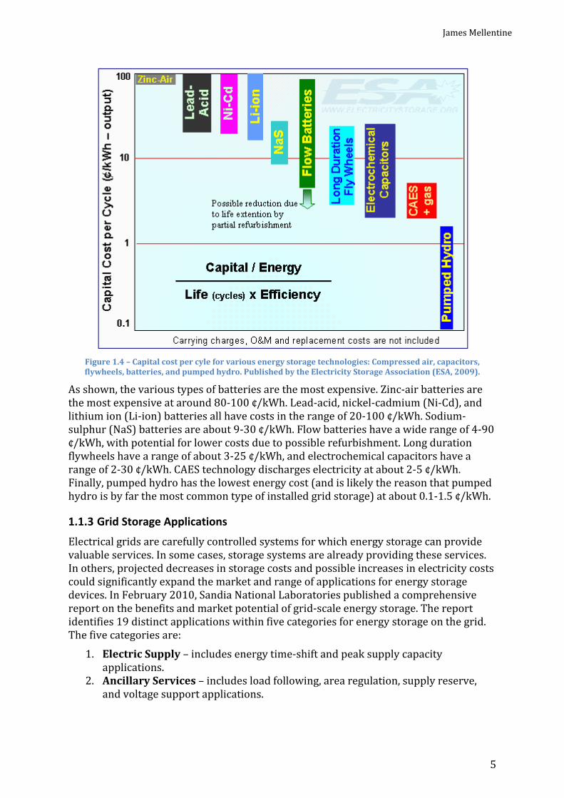
List of Figures Figure 1.1 – System ratings of various energy storage technologies: Compressed air, capacitors, flywheels, batteries, and pumped hydro. Published by the Electricity Storage Association (ESA, 2009). .................................................................................................................................................................................... 2 Figure 1.2 – Specific energy and specific power of various energy storage technologies: Capacitors, flywheels, batteries, and fuel cells. Published by The Electropaedia (The Electropaedia, 2005). ...................................................................................................................................................... 3 Figure 1.3 – Cost per kW and per kWh for various energy storage technologies: Compressed air, capacitors, flywheels, batteries, and pumped hydro. Published by the Electricity Storage Association (ESA, 2009). ................................................................................................................................................ 4 Figure 1.4 – Capital cost per cyle for various energy storage technologies: Compressed air, capacitors, flywheels, batteries, and pumped hydro. Published by the Electricity Storage Association (ESA, 2009). ................................................................................................................................................ 5 Figure 1.5 – The benefits and maximum market potential for each of the 19 applications identified for grid-scale storage in the Sandia report (Eyer & Corey, 2010). .......................................... 7 Figure 1.6 – Diagram of an iron hybrid flow battery including system components and electrochemical reactions. ............................................................................................................................................ 8 Figure 1.7 – Cost breakdown of a 2 kW, 30 kWh vanadium redox flow battery system, based on a manufacturing volume of 1700 units. The vanadium pentoxide (V2O5) is by far the largest component cost at 43%. (Joerissen, Garche, Fabjan, & Tomazic, 2004). ................................................ 10 Figure 1.8 – Cost breakdown of a 2 kW, 300 kWh vanadium redox flow battery system, based on a manufacturing volume of 1700 units. The vanadium pentoxide (V2O5) is by far the largest component cost at 81%. (Joerissen, Garche, Fabjan, & Tomazic, 2004). ................................................ 10 Figure 1.9 – The average market price for vanadium pentoxide from 2005 to present shows its volatile and relatively expensive nature (USGS, 2010) (MinorMetals.com, 2010). ........................... 11 Figure 1.10 – The daily load profile of the rural feeder line in Castle Valley Utah. The pink solid line shows the normal line load without energy storage. The blue dashed line shows the line load with the vanadium flow battery installed – it shaves the peak to be within the capacity limit of the electricity lines, thus allowing for continued demand increase while deferring expensive infrastructure upgrades (Kuntz, 2005). ............................................................................................................... 13 Figure 2.1 – Bifunctional redox flow battery concept (Wen Y. H., Cheng, Ma, & Yang, 2008). ...... 24 Figure 2.2 – The open circuit voltage of the iron hybrid flow battery versus state of charge. ...... 26 Figure 3.1 – Pressure drop measurements versus linear flow rate for different felt thicknesses. This figure is from a study published in the Journal of Industrial & Engineering Chemistry Research (Gonzalez-Garcia, Montiel, Aldaz, Conesa, Perez, & Codina, 1998)....................................... 31 Figure 3.2 – An example distribution of component prices. The x-axis is the estimated component price, and the y-axis is the probability of each price being the real price. Price “a” is an optimistic (low) price, Price “m” is the most likely price (highest probability), and Price “b” is a pessimistic (high) price. .......................................................................................................................................... 39 Figure 3.3 – Individual component costs as a percent of total system cost for a 10 kW, 20.9 kWh iron hybrid flow battery system. The largest costs of the system are the activated felt, bipolar plates, and flow frames. The cost of electrolyte and preparation is about 3% of the total cost. .. 41 Figure 3.4 – The sensitivity of the system cost per kW based on the variation of each expected component price is shown. The unit price of the activated felt, bipolar plates, and flow frames are shown to have the greatest impact on cost per kW. Other unit prices have only a slight effect. ............................................................................................................................................................................................... 42

vi
Figure 3.5 - The sensitivity of the system cost per kWh based on the variation of each expected component price is shown. The unit price of the activated felt, bipolar plates, and flow frames are shown to have the greatest impact on cost per kWh. Other unit prices have only a slight effect. ................................................................................................................................................................................... 43 Figure 3.6 – The sensitivity of the system cost per kW based on the variation of four performance factors is shown. The improvement of the current density and voltaic efficiency are shown to have the greatest impact on cost per kW. An increasing iron concentration would have only a slight impact on cost, while an increase in plating density would actually increase the cost per kW slightly due to increased electrolyte volume. .................................................................................... 44 Figure 3.7 - The sensitivity of the system cost per kWh based on the variation of five performance factors is shown. The improvement of the plating density, coulombic efficiency, and voltaic efficiency are shown to have the greatest impact on cost per kWh. An increasing iron concentration would have only a slight impact on cost, while an increase in current density would actually increase the cost per kWh slightly due to decreased active area available for plating. ................................................................................................................................................................................ 45 Figure 3.8 – the per kW and per kWh costs for the iron hybrid flow battery are compared to the vanadium redox flow battery, zinc bromine hybrid flow battery, and other energy storage systems. ............................................................................................................................................................................. 47 Figure 4.1 – Visual example of how area regulation services are applied to the load curve. This diagram comes from a study by Sandia National Laboratory (Eyer & Corey, 2010). ....................... 50 Figure 4.2 – The amount of up and down regulation capacity purchased by CAISO in 2008, per hour (CAISO, 2009). ...................................................................................................................................................... 52 Figure 4.3 – The purchase price paid for 1 MW of up regulation capacity per hour in 2008 (CAISO, 2009). ................................................................................................................................................................. 53 Figure 4.4 – The purchase price paid for 1 MW of down regulation capacity per hour in 2008 (CAISO, 2009). ................................................................................................................................................................. 53 Figure 4.5 – The state of charge of an iron hybrid flow battery over the course of a year in an area regulation application. The average state of charge is 41.4%. ......................................................... 55 Figure 4.6 – Distribution of annual area regulation revenue received by a 2 MW iron hybrid flow battery, based on 1000 simulations of random charge/discharge operations per hour. ............... 56 Figure 4.7 – Distribution of net revenue minus energy costs received by a 2 MW iron hybrid flow battery operating at 64% energy efficiency, based on 1000 simulations of random charge/discharge operations per hour. ............................................................................................................... 56 Figure 4.8 – Distribution of net revenue minus energy costs received by a 2 MW iron hybrid flow battery operating at 75% energy efficiency, based on 1000 simulations of random charge/discharge operations per hour. ............................................................................................................... 57 Figure 5.1 – A schematic diagram of the lab station used for the performance testing of an iron hybrid flow battery. ...................................................................................................................................................... 59 Figure 5.2 – Photograph of 50 cm2 cell used for experiments. The left photo is the assembled cell with all layers. The smaller right-side photos are cross-sectional views of each layer. The numbered labels correspond to: 1) Flow block, 2) Non-conducting Teflon layer, 3) Gold-plated copper conductor, 4) Grafoil layer 5) Graphite electrode, 6) PVC spacer & activated felt layer, 7) Membrane, 8) Negative electrolyte inlet, and 9) Positive electrolyte outlet. ....................................... 61 Figure 5.3 – Data from cycle 69 is shown as the noisy raw data (blue line) and as the smoothed data (red line). The smoothed data has had a median filter algorithm applied with a window size of 121. ................................................................................................................................................................................. 67

vii
Figure 5.4 – The estimated electrolyte crossover rate observed during symmetric cell tests using the microporous membrane. Positive rates indicate electrolyte transfer from the rear tank to the front tanks. Negative rates indicate the opposite, electrolyte transferring from the front tank to the rear tank. ................................................................................................................................................................... 71 Figure 5.5 – Theoretical open circuit (equilibrium) potential of the symmetric cell. ....................... 72 Figure 5.6 – Voltage curves from the symmetric cell cycles 1-7 using the Celgard 5550 PP membrane and NH4Cl as the supporting electrolyte salt, and a current density of 50 mA/cm2. . 72 Figure 5.7 – A zoomed view of the voltage curves from cycles 2, 3, 5, 6, and 7. The voltage behavior shows consistency and repeatability through about 150 minutes at 50 mA/cm2. ......... 73 Figure 5.8 – Voltage curves from the symmetric cell cycles 8-13 using the Celgard 5550 PP membrane and NH4Cl as the supporting electrolyte salt, and a current density of 100 mA/cm2.74 Figure 5.9 - A zoomed view of the voltage curves from cycles 8-13. The voltage behavior shows consistency and repeatability through about 75 minutes at 100 mA/cm2. .......................................... 75 Figure 5.10 - Voltage curves from symmetric cell cycles 31-38 using the Nafion 1135 membrane and NH4Cl as the supporting electrolyte salt. The current density was 50 mA/cm2. Marked deterioration in performance was observed starting with cycle 34. ....................................................... 76 Figure 5.11 - Voltage curves from symmetric cell cycles 39-44 using the Nafion 1035 membrane and NaCl as the supporting electrolyte salt. The current density was 50 mA/cm2. Voltage behavior was steady and repeatable. .................................................................................................................... 77 Figure 5.12 - Voltage curves from symmetric cell cycles 45-50 using the Nafion 1035 membrane and NaCl as the supporting electrolyte salt. The current density was 100 mA/cm2. Voltage behavior was steady and repeatable. .................................................................................................................... 78 Figure 5.13 - Voltage curves from symmetric cell cycles 51-56 using the Nafion 1035 membrane and NaCl as the supporting electrolyte salt. The current density was 200 mA/cm2. Voltage behavior was steady and repeatable. .................................................................................................................... 79 Figure 5.14 - Voltage curves from symmetric cell cycles 57-62 using the Nafion 1035 membrane and NaCl as the supporting electrolyte salt. The current density was 300 mA/cm2. Voltage behavior was steady and repeatable. .................................................................................................................... 80 Figure 5.15 - Voltage curves from symmetric cell cycles 63-68 using the Nafion 1035 membrane and NaCl as the supporting electrolyte salt. The current density was 400 mA/cm2. Voltage behavior was steady and repeatable. .................................................................................................................... 80 Figure 5.16 - Voltage curves from cycles 69 & 70 using the Nafion 1035 membrane and NaCl as the supporting electrolyte salt. The current density was 20 mA/cm2 and the plating density was 50 mA-hr/cm2. The voltage curves show similar shapes, with cycle 70 showing a longer discharge time. ................................................................................................................................................................ 82 Figure 5.17 - Voltage curves from cycles 71 & 72 using the Nafion 1035 membrane and NaCl as the supporting electrolyte salt. The current density was 20 mA/cm2 and the attempted plating density was 100 mA-hr/cm2. A plating density of only 61.3 mA-hr/cm2 was reached on cycle 71 before the upper voltage limit was reached. ...................................................................................................... 83 Figure 5.18 – Calculated efficiencies for cycles 69-72. Voltaic efficiency values declined through the 4 cycles from 76.4% to 66.4%. The coulombic efficiency showed less consistency, starting at 43.0%, rising to as much as 86.5%, and then falling again to 70.7%. Energy efficiencies showed a similar pattern, 32.9% and 63.5% being the lowest and highest values, respectively. ................... 83 Figure 5.19 – Voltage curves from cycles 73-74 and 89-90 using the Nafion 1035 membrane and NaCl as the supporting electrolyte salt. The current density was 35 mA/cm2 and the plating density was 50 mA-hr/cm2. ....................................................................................................................................... 85

viii
Figure 5.20 – Voltage curves from cycles 91 and 92 using the Nafion 1035 membrane and NaCl as the supporting electrolyte salt. The current density was 35 mA/cm2 and the plating density was 100 mA-hr/cm2. .................................................................................................................................................... 85 Figure 5.21 – Calculated efficiencies for cycles 73-74 and 89-92. Overall, efficiencies were relatively low on cycles 73-74. Efficiencies increased with the introduction of a new electrolyte and membrane in cycle 89, and then declined significantly with higher plating densities of cycle 91 and 92. ......................................................................................................................................................................... 86 Figure 5.22 – Voltage curves from cycles 82-83 using the Nafion 1135 membrane and NaCl as the supporting electrolyte salt. The current density was 50 mA/cm2 and the plating density was 50 mA-hr/cm2. ................................................................................................................................................................ 87 Figure 5.23 – Voltage curves from cycles 84-85 using the Nafion 1135 membrane and NaCl as the supporting electrolyte salt. The current density was 50 mA/cm2 and the plating density was an attempted 100 mA-hr/cm2. Cycle 85 did not achieve this plating density due to prematurely reaching preset voltage limits. ................................................................................................................................. 87 Figure 5.24 – Calculated efficiencies for cycles 82-85. Voltaic efficiency values declined through the 4 cycles from 68.2% to 41.5%. The coulombic efficiencies were 69.6% and 88.9% at the lower plating density and 54.2% at the higher plating density, while the final shorter cycle was 95.7%. Energy efficiencies showed a similar pattern, 47.5% and 54.1% in the first two cycles and 26.1% in cycle 84, and finally 39.7% in the short cycle 85. ................................................................ 88 Figure 5.25 – Voltage curves from cycles 93 and 94 using the Nafion 1035 membrane and NaCl as the supporting electrolyte salt. The current density was 65 mA/cm2 and the plating density was 50 mA-hr/cm2. ....................................................................................................................................................... 89 Figure 5.26 – Voltage curves from cycles 95 and 96 using the Nafion 1035 membrane and NaCl as the supporting electrolyte salt. The current density was 65 mA/cm2 and the plating density was 100 mA-hr/cm2. .................................................................................................................................................... 90 Figure 5.27 – The efficiencies calculated from this set of data are much more consistent over 4 consecutive cycles than with other cycles, even if the overall performance is lower. This may be due to avoidance of buildup on the membrane with the addition of an inert (PP) felt material in the cell. ............................................................................................................................................................................... 90 Figure 5.28 – Voltage curve from cycle 97 using the Nafion 1035 membrane and NaCl as the supporting electrolyte salt. The current density was 80 mA/cm2 on charge and 50 mA/cm2 on discharge. The plating density was 50 mA-hr/cm2. ........................................................................................ 91 Figure 5.29 – Voltage curve from cycle 98 using the Nafion 1035 membrane and NaCl as the supporting electrolyte salt. The current density was 50 mA/cm2 on charge and 20 mA/cm2 on discharge. The plating density was 100 mA-hr/cm2. ..................................................................................... 92 Figure 5.30 – Calculated power densities for charge and discharge cycles for varying current densities discussed in this chapter. ........................................................................................................................ 93 Figure 5.31 – Calculated energy densities based on volume and mass for charge and discharge cycles for varying current densities discussed in this chapter. .................................................................. 93
ix
List of Tables Table 1.1 - Descriptions and examples of the primary grid storage technologies ................................ 1 Table 1.2 – Possible applications for grid-scale energy storage, along with power and discharge time requirements. Data sourced from a Sandia National Laboratories report (Eyer & Corey, 2010). .................................................................................................................................................................................... 6 Table 3.1 – Assumed system and performance characteristics of an iron hybrid flow battery system. Subsequent system design and performance characteristics were calculated from these assumptions. .................................................................................................................................................................... 27 Table 3.2 – Calculated system and performance characteristics for a 10 kW/20.9 kWh iron flow battery system. ............................................................................................................................................................... 33 Table 3.3 – A summarized list of components considered for the cost estimation of an iron hybrid flow battery. The annual quantity of each component is presented based on a production of 1000 units/year. The pessimistic, most likely, and optimistic unit costs are shown for each component. ....................................................................................................................................................................... 38 Table 3.4 – For each component of the iron hybrid flow battery system, the calculated values of expected cost, standard deviation, and variance are shown. These values are based on the Three Point Estimation method. ........................................................................................................................................... 40 Table 4.1 – After removing several applications from Table 1.2 based on discharge time requirements, this is a list of possible applications for an iron hybrid flow battery, Data sourced from a Sandia National Laboratories report (Eyer & Corey, 2010). ......................................................... 49 Table 4.2 – A summary of assumptions made for the performance analysis of an iron hybrid flow battery in an area regulation application. ........................................................................................................... 52 Table 4.3 – Summary of calculated performance metrics for a 2 MW iron hybrid flow battery performing in a hypothetical area regulation application at 55% energy efficiency. ....................... 57 Table 5.1 – The general physical properties of the six membrane separator materials that were used in the course of experiments with an iron hybrid flow battery (Celgard, 2010) (Daramic, 2000). ................................................................................................................................................................................. 63 Table 5.2 – The cycles are shown for the symmetric cell tests, along with current density and pump flow rate for each cycle. Cycles 1-13 were conducted with microporous membrane. Cycles 31-68 were conducted with Nafion membrane. ............................................................................................... 65 Table 5.3 – Cycle numbers for cell performance testing, along with charge current density, discharge current density, pump flow rate, intended plating density (which was not always achieved during the tests), and the charge/discharge time limits entered into the VI control panel. ................................................................................................................................................................................... 66 Table 5.4 – Electrolyte solution properties used in this study, and the battery cycles in which each was used. Included are the total volume and mass of the electrolyte batch, along with the concentration of each chemical used and the recorded pH. Note the total volume is the combined volume of both positive and negative electrolytes. For batches 12-15, this was split as a 2:1 ratio between positive and negative tanks. ............................................................................................. 70 Table 5.5 – A summary of measured data and calculated performance values for the cycles discussed in this section. ............................................................................................................................................ 94 Table 5.6 – A summary of the primary assumed performance values compared to the actual observed performance values for an iron hybrid flow battery. ................................................................. 95 Table 6.1 – Summary of assumed and calculated design parameters for the 10 kW modular iron hybrid flow battery. ...................................................................................................................................................... 99

x
Table 6.2 – Summary of components of an iron hybrid flow battery system, along with annual required quantities and estimated unit costs assuming 1000 units of annual production. ......... 100 Table 6.3 – Summary of assumed and calculated simulation parameters for a 2 MW iron hybrid flow battery system performing an area regulation application. ............................................................ 101 Table 6.4 – Summary of maximum and average observed performance characteristics of the single-cell 50 cm2 iron hybrid flow battery. ..................................................................................................... 103

James Mellentine
1
Chapter 1: Introduction Worldwide electrical grid storage capacity is estimated at 128 GW, less than 3% of total grid capacity. ABI Research expects that to grow to 150 GW by 2015 (ABI Research, 2010). According to a recent report published by Sandia National Laboratories “electric energy storage is poised to become an important element of the electricity infrastructure of the future” and details several value propositions. The Sandia report also notes major challenges to implementation, among them the relatively high cost of storage relative to the benefits (Eyer & Corey, 2010). This chapter introduces the topic of this thesis. The following sections begin with a comparison of various grid storage options, while highlighting the performance and cost characteristics of flow batteries. An introduction to flow battery technology is presented along with a description of the iron-based electrolyte that is the subject of this thesis. The chapter concludes with a description of the thesis objective. 1.1 Grid Energy Storage Technologies There are seven primary categories of electricity storage technology: pumped hydropower, compressed air energy storage (CAES), electrochemical batteries, capacitors, flywheels, superconducting magnetic energy storage (SMES), and thermal energy storage. A short description of each of these technologies along with an example is shown in Table 1.1. Table 1.1 - Descriptions and examples of the primary grid storage technologies
Technology Description Example
Pumped Hydro Turbines are used to pump water from a lower water reservoir to a higher reservoir during off-peak periods. The water is then released back through the turbines to the lower reservoir to generate electricity during peak periods.
Goldisthal, Germany; 1060 MW/7500 MWh (Beyer, 2007) CAES During off-peak periods, low-price electricity is used to compress air into large geological cavities. The compressed air is then released as an input into a natural gas peaking plant during peak demand.
McIntosh, Alabama; 110 MW peak/26 hours storage (Daniel, 2009) Battery Electrical energy is converted into chemical energy through a chemical reaction, which is then reversed during discharge of the battery. Castle Valley, Utah; 250 kW/2 MWh (EPRI, 2007)
Capacitor Electrical energy is stored as a physical charge on opposing electrodes, allowing for rapid charge & discharge. Maxwell Technologies; bridge power for telecommunications backup (Maxwell Technologies) Flywheel Electricity is used to spin a flywheel at very high speed with very low frictional losses. When needed, the flywheel spins a generator to put electricity back into the grid. Stephenstown, NY; 20 MW (Beacon Power, 2010)
SMES Electricity is stored as energy in a magnetic field, typically with superconducting metals at very low temperatures. Northern Wisconsin; Grid Stability, 2 MW (American Superconductor) Thermal Heat energy stored in a solid, liquid, or gas material can be used to generate electricity directly through a thermocouple or indirectly through the conventional Rankine cycle. Southern Spain; 50 MW/375 MWh (Solar Millennium, 2008)

Chapter 1: Introduction
2
1.1.1 Storage Performance Comparison Each energy storage technology varies in terms of power and energy capacity. These capacities are key indicators of what applications a storage medium might be able to fulfill. For example, a low-power & high-energy storage device (i.e. longer discharge time) might be appropriate for on-site auxiliary or supplementary power, whereas a high-power & low-energy storage device (i.e. shorter discharge time) might be more appropriate for grid-scale power quality regulation. Based on data from installed storage systems as of November 2008, the Electricity Storage Association created a graph that compares the power capacity and discharge time of various technologies, as shown in Figure 1.1 (ESA, 2009).
Figure 1.1 – System ratings of various energy storage technologies: Compressed air, capacitors, flywheels,
batteries, and pumped hydro. Published by the Electricity Storage Association (ESA, 2009). As shown in the logarithmic graph, pumped hydropower generally has relatively high power (~400 MW-2000 MW) and discharge time (~20 hr-100 hr) capacities when compared to other storage technologies. Compressed air systems generally have less power (~2 MW-300 MW) and discharge time (~2 hr-30 hr) capacities than pumped hydro, but more than other technologies. Batteries have a wide range of performance ratings depending on the specific technology and electrolyte chemistry, with installed systems having power ranges of anywhere from ~7 kW-80 MW and discharge times of a few seconds to 20 hours. Flywheel storage performance lies within the bounds of battery performance, in the mid-range of power (~0.1 MW-10 MW) and the low end of discharge time (a few seconds to almost an hour. Finally, capacitor storage systems have the lowest relative discharge time (fractions of a second to a few seconds) and mid-range power (~0.7 MW-3 MW).

James Mellentine
3
Energy storage can also be characterized by energy and power density. Large and heavy storage options are generally relegated to stationary applications such as grid storage, while smaller and lighter storage options may be attractive for non-stationary uses such as transportation. Figure 1.2 shows a graph of specific energy (Wh/kg) vs. specific power (W/kg) of various energy storage technologies (The Electropaedia, 2005).
Figure 1.2 – Specific energy and specific power of various energy storage technologies: Capacitors, flywheels,
batteries, and fuel cells. Published by The Electropaedia (The Electropaedia, 2005). As shown in the logarithmic graph, fuel cells are the most energy dense (~50 Wh/kg -300 Wh/kg) and least power dense (~1 W/kg - 60 W/kg) of the technologies shown. Batteries have the second highest specific energy (~5 Wh/kg – 60 Wh/kg) and second lowest specific power (~2 W/kg – 60 W/kg). Flywheels have a small mid-range specific energy (~4 Wh/kg – 30 Wh/kg) and specific power (~0.1 kW/kg – 5 kW/kg). Double-layer capacitors have a wide mid-range specific energy (~0.8 Wh/kg – 5 Wh/kg) and specific power (~3 W/kg – 60 kW/kg). SMES has the smallest range of specific energy (~0.1 Wh/kg – 0.4 Wh/kg) and specific power (~0.5 kW/kg – 4 kW/kg). Finally, standard capacitors are the least energy dense (~0.02 Wh/kg – 0.09 Wh/kg) and most power dense (~3 kW/kg – 10 MW/kg) of the technologies shown. 1.1.2 Cost Comparison The cost of energy storage on a per kW and per kWh basis is a key consideration for customers. Except for pumped hydropower, grid-scale storage has traditionally been more costly than the marginal cost of peak generation. This is why we have “peaking plants” instead of “peaking storage” to provide electricity for the small fraction of the time when demand is highest. Based on 2002 market data and projections for the near future, the ESA compiled and graphed energy storage cost data, shown in Figure 1.3. This figure shows a graph of capital cost per unit power ($/kW) vs. capital cost per unit energy ($/kWh) for a variety of energy storage technologies (ESA, 2009).

Chapter 1: Introduction
4
Figure 1.3 – Cost per kW and per kWh for various energy storage technologies: Compressed air, capacitors,
flywheels, batteries, and pumped hydro. Published by the Electricity Storage Association (ESA, 2009). This logarithmic graph shows that costs vary widely. High-power electrochemical capacitors have the highest per kWh cost (~$4000/kWh - $10,000/kWh) and the lowest per kW cost (~$100/kW - $450/kW). High-power flywheels have the second highest per kWh cost (~$2500/kWh - $4500/kWh) and a low per kW cost (~$200/kW - $600/kW). Long-duration flywheels are slightly lower in energy cost (~$1000/kWh - $3000/kWh), but are the highest power cost (~$3000/kW - $10,000/kW). Excluding the metal-air outlier, batteries have a wide mid-range cost for both energy (~$100/kWh - $2500/kWh) and power (~$350/kW - $5000/kW). Long-duration electrochemical capacitors also have a mid-range energy cost (~$100/kWh - $250/kWh), but a low-end power cost (~$250/kW - $500/kW). Pumped hydro storage has one of the lowest per kWh cost (~$40/kWh - $200/kWh) and a mid-range per kW cost (~$500/kW - $1500/kW). Finally, CAES has a similarly low energy cost (~$30/kWh - $100/kWh) and a low power cost (~$450/kW - $1000/kW). For applications that involve frequent charge & discharge cycles, it is helpful to evaluate the cost of energy storage on a per-kWh and per-cycle basis. This essentially takes the overall cost per kWh (presented in Figure 1.3) and divides it by the number of expected life cycles and the round-trip energy efficiency of the technology. This can be considered the equivalent to the levelized cost of electricity that is calculated for electricity generation technologies. For the same storage technologies as above, the ESA calculated the capital cost per cycle ($/kWh/cycle), shown in Figure 1.4. Note that carrying charges, operations and maintenance (O & M) costs, and replacement costs are not included in this data.
James Mellentine
5
Figure 1.4 – Capital cost per cyle for various energy storage technologies: Compressed air, capacitors, flywheels, batteries, and pumped hydro. Published by the Electricity Storage Association (ESA, 2009). As shown, the various types of batteries are the most expensive. Zinc-air batteries are the most expensive at around 80-100 ¢/kWh. Lead-acid, nickel-cadmium (Ni-Cd), and lithium ion (Li-ion) batteries all have costs in the range of 20-100 ¢/kWh. Sodium-sulphur (NaS) batteries are about 9-30 ¢/kWh. Flow batteries have a wide range of 4-90 ¢/kWh, with potential for lower costs due to possible refurbishment. Long duration flywheels have a range of about 3-25 ¢/kWh, and electrochemical capacitors have a range of 2-30 ¢/kWh. CAES technology discharges electricity at about 2-5 ¢/kWh. Finally, pumped hydro has the lowest energy cost (and is likely the reason that pumped hydro is by far the most common type of installed grid storage) at about 0.1-1.5 ¢/kWh.
1.1.3 Grid Storage Applications Electrical grids are carefully controlled systems for which energy storage can provide valuable services. In some cases, storage systems are already providing these services. In others, projected decreases in storage costs and possible increases in electricity costs could significantly expand the market and range of applications for energy storage devices. In February 2010, Sandia National Laboratories published a comprehensive report on the benefits and market potential of grid-scale energy storage. The report identifies 19 distinct applications within five categories for energy storage on the grid. The five categories are: 1. Electric Supply – includes energy time-shift and peak supply capacity applications. 2. Ancillary Services – includes load following, area regulation, supply reserve, and voltage support applications.

Chapter 1: Introduction
6
3. Grid System – includes transmission support, transmission congestion relief, transmission and distribution (T & D) upgrade deferral, and substation on-site power applications. 4. End User/Utility Customer – includes time-of-use cost management, demand charge management, electric service reliability, and power quality applications. 5. Renewables Integration – includes renewable energy time-shift, capacity firming, and wind generation grid integration applications. Each application has different power and discharge time requirements. Table 1.2 summarizes these requirements as specified by the Sandia report (Eyer & Corey, 2010). Table 1.2 – Possible applications for grid-scale energy storage, along with power and discharge time requirements. Data sourced from a Sandia National Laboratories report (Eyer & Corey, 2010).
Application Power Discharge Time # Description Low High Low High 1 Electric Energy Time Shift 1 MW 500 MW 2 hr. 8 hr. 2 Electric Supply Capacity 1 MW 500 MW 4 hr. 6 hr. 3 Load Following 1 MW 500 MW 2 hr. 4 hr. 4 Area Regulation 1 MW 40 MW 15 min. 30 min.5 Electric Supply Reserve Capacity 1 MW 500 MW 1 hr. 2 hr. 6 Voltage Support 1 MW 10 MW 15 min. 1 hr. 7 Transmission Support 10 MW 100 MW 2 sec. 5 sec. 8 Transmission Congestion Relief 1 MW 100 MW 3 hr. 6 hr. 9.1 Transmission & Distribution Upgrade (50th Percentile) 250 kW 5 MW 3 hr. 6 hr. 9.2 Transmission & Distribution Upgrade (90th Percentile) 250 kW 2 MW 3 hr. 6 hr. 10 Substation On-site Power 1.5 kW 5 kW 8 hr. 16 hr. 11 Time-of-use Energy Cost Management 1 kW 1 MW 4 hr. 6 hr. 12 Demand Charge Management 50 kW 10 MW 5 hr. 11 hr. 13 Electric Service Reliability 0.2 kW 10 MW 5 min. 1 hr. 14 Electric Service Power Quality 0.2 kW 10 MW 10 sec. 1 min. 15 Renewable Energy Time-shift 1 kW 500 MW 3 hr. 5 hr. 16 Renewables Capacity Firming 1 kW 500 MW 2 hr. 4 hr. 17.1 Wind Generation Grid Integration, Short Duration 0.2 kW 500 MW 10 sec. 15 min.
17.2 Wind Generation Grid Integration, Long Duration 0.2 kW 500 MW 1 hr. 6 hr. The Sandia report also includes a market analysis for each application. The report quantifies the potential monetary benefit (in $/kW) over the next 10 years as well as the maximum market potential (in MW) over the next 10 years. In theory, a storage system that costs less to produce than the proposed monetary benefit would save the

James Mellentine
7
customer money, and thereby creates a market opportunity. Figure 1.5 shows a graph of the potential monetary benefit and maximum market potential for each storage application identified (Eyer & Corey, 2010).
Figure 1.5 – The benefits and maximum market potential for each of the 19 applications identified for grid-
scale storage in the Sandia report (Eyer & Corey, 2010).
1.2 Flow Battery Technology A flow battery is a rechargeable battery that uses electrolytes moving (“flowing”) through an electrochemical cell to convert chemical energy from the electrolyte into electricity (and vice versa when charging). The electrolytes used in flow batteries are generally composed of ionized metal salts in an acidic solution. Some of the most commonly used elements in commercial flow battery systems are zinc, bromine, and vanadium. Unlike a traditional battery, the electrodes do not take part in the reactions, and the actual cell where the electrochemical reactions take place is small. The electrolytes are stored in large external tanks and are pumped through each side of the cell according to the charge/discharge current applied. Like traditional batteries, cells are “stacked” together in a flow battery system to achieve the desired power output. Since the electrolyte is stored externally, the amount energy that can be stored by a flow battery is largely determined by the solubility of the chemicals and the size of the tanks and the latter can be easily scaled by changing the size of the tanks. In the case of a hybrid flow battery, the subject of this study, energy capacity is also limited by the amount of metal that can be plated onto the electrode, so the electrode surface area also

Chapter 1: Introduction
8
affects the energy capacity of a hybrid flow battery. Flow battery system components and costs are discussed further in this section. 1.2.1 System Components Figure 1.6 shows a conceptual diagram of a basic single-cell flow battery (in this case the iron hybrid flow battery that is the subject of this study), with labels for the various components of the system.
Figure 1.6 – Diagram of an iron hybrid flow battery including system components and electrochemical
reactions. The two electrolyte storage tanks are represented as cylinders on the sides of the diagram. The tank on the negative electrode holds ferrous chloride (FeCl2) in solution, and the positive tank holds a mixture of ferrous chloride and ferric chloride (FeCl3) in solution, with proportions depending on the state of charge. The components and preparation method of the electrolyte can significantly impact the overall cost of the flow battery. Low cost raw materials and low-cost electrolyte preparation methods are desirable. There are pumps on each side of the cell, shown on the bottom of the diagram. These pumps force the fluid electrolytes through the cell. In order to achieve steady and controllable performance from the battery, the pump speeds are generally set at a rate that is a multiple stoichiometric rate of reaction of the cell. A negative effect of the pumps is that they create a parasitic load on the battery, reducing the overall efficiency. The cell structure is enclosed by bipolar plates. Bipolar plates serve a dual purpose as both structural support and conductor. In the case of stacked cells, the bipolar plates are in between each cell and serve as both a cathode for one cell and an anode for the other. These plates also conduct waste heat out of the cell. Important properties of the bipolar plates are strength, electronic conductivity, separation of electrolytes, corrosion resistance, and inexpensive manufacturing. Inside the cell and next to the bipolar plate on each side is an electrode. In the case of the subject iron flow battery, the electrodes are graphite. The electrodes do not take place in the electrochemical reactions, but they provide a surface on which it can take
James Mellentine
9
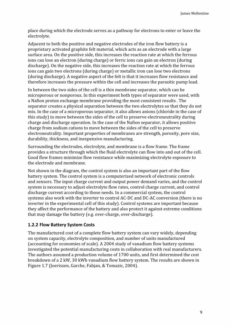
place during which the electrode serves as a pathway for electrons to enter or leave the electrolyte. Adjacent to both the positive and negative electrodes of the iron flow battery is a proprietary activated graphite felt material, which acts as an electrode with a large surface area. On the positive side, this increases the reaction rate at which the ferrous ions can lose an electron (during charge) or ferric ions can gain an electron (during discharge). On the negative side, this increases the reaction rate at which the ferrous ions can gain two electrons (during charge) or metallic iron can lose two electrons (during discharge). A negative aspect of the felt is that it increases flow resistance and therefore increases the pressure within the cell and increases the parasitic pump load. In between the two sides of the cell is a thin membrane separator, which can be microporous or nonporous. In this experiment both types of separator were used, with a Nafion proton exchange membrane providing the most consistent results . The separator creates a physical separation between the two electrolytes so that they do not mix. In the case of a microporous separator, it also allows anions (chloride in the case of this study) to move between the sides of the cell to preserve electroneutrality during charge and discharge operation. In the case of the Nafion separator, it allows positive charge from sodium cations to move between the sides of the cell to preserve electroneutrality. Important properties of membranes are strength, porosity, pore size, durability, thickness, and inexpensive manufacturing. Surrounding the electrodes, electrolyte, and membrane is a flow frame. The frame provides a structure through which the fluid electrolyte can flow into and out of the cell. Good flow frames minimize flow resistance while maximizing electrolyte exposure to the electrode and membrane. Not shown in the diagram, the control system is also an important part of the flow battery system. The control system is a computerized network of electronic controls and sensors. The input charge current and output power demand varies, and the control system is necessary to adjust electrolyte flow rates, control charge current, and control discharge current according to those needs. In a commercial system, the control systems also work with the inverter to control AC-DC and DC-AC conversion (there is no inverter in the experimental cell of this study). Control systems are important because they affect the performance of the battery and also protect it against extreme conditions that may damage the battery (e.g. over-charge, over-discharge). 1.2.2 Flow Battery System Costs The manufactured cost of a complete flow battery system can vary widely, depending on system capacity, electrolyte composition, and number of units manufactured (accounting for economies of scale). A 2004 study of vanadium flow battery systems investigated the potential manufacturing costs in collaboration with real manufacturers. The authors assumed a production volume of 1700 units, and first determined the cost breakdown of a 2 kW, 30 kWh vanadium flow battery system. The results are shown in Figure 1.7 (Joerissen, Garche, Fabjan, & Tomazic, 2004).
Chapter 1: Introduction
10
Figure 1.7 – Cost breakdown of a 2 kW, 30 kWh vanadium redox flow battery system, based on a
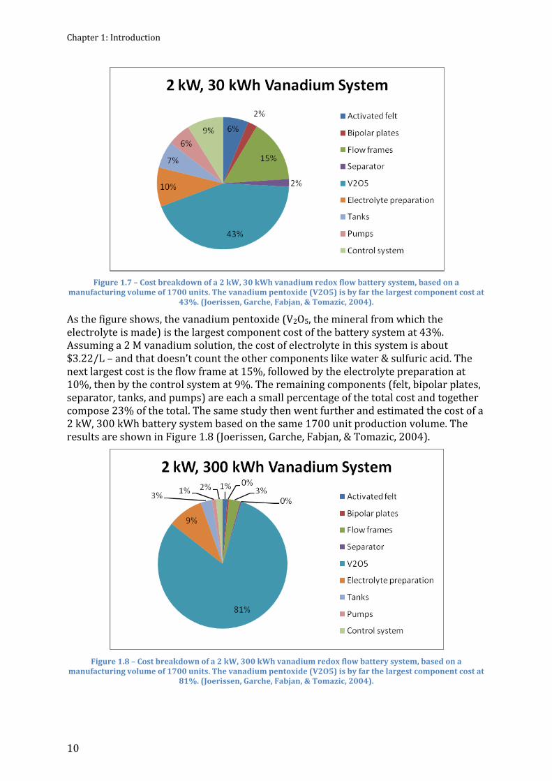
manufacturing volume of 1700 units. The vanadium pentoxide (V2O5) is by far the largest component cost at 43%. (Joerissen, Garche, Fabjan, & Tomazic, 2004). As the figure shows, the vanadium pentoxide (V2O5, the mineral from which the electrolyte is made) is the largest component cost of the battery system at 43%. Assuming a 2 M vanadium solution, the cost of electrolyte in this system is about $3.22/L – and that doesn’t count the other components like water & sulfuric acid. The next largest cost is the flow frame at 15%, followed by the electrolyte preparation at 10%, then by the control system at 9%. The remaining components (felt, bipolar plates, separator, tanks, and pumps) are each a small percentage of the total cost and together compose 23% of the total. The same study then went further and estimated the cost of a 2 kW, 300 kWh battery system based on the same 1700 unit production volume. The results are shown in Figure 1.8 (Joerissen, Garche, Fabjan, & Tomazic, 2004).
Figure 1.8 – Cost breakdown of a 2 kW, 300 kWh vanadium redox flow battery system, based on a
manufacturing volume of 1700 units. The vanadium pentoxide (V2O5) is by far the largest component cost at 81%. (Joerissen, Garche, Fabjan, & Tomazic, 2004).

James Mellentine
11
In this system, it is clear that the dominating cost of the system is from the vanadium pentoxide at 81% of the total cost. Assuming a 2 M vanadium solution, the cost of electrolyte in this system is the same as above, $3.22/L, not counting water & sulfuric acid. The next highest cost comes from the electrolyte preparation at 9%. All other battery components together compose 10% of the total cost (Joerissen, Garche, Fabjan, & Tomazic, 2004). As the energy capacity of the battery increases, more electrolyte is needed and more V2O5 is required. As shown in this example, the electrolyte is clearly the most important driver behind the cost of the vanadium flow battery. If a similar flow battery could be manufactured with a less expensive electrolyte, then the overall cost of the battery could be significantly decreased. To get a sense of how much the cost of electrolyte source-minerals vary, a simple resource assessment and market survey follows for the minerals used in the primary commercial flow battery chemistries – zinc-bromine and vanadium – and for the iron chemistry that is the subject of this study. Relatively rare, vanadium has a global resource of 63 million metric tons, with the vast majority of vanadium pentoxide (V2O5) mines in China, Russia, and South Africa (USGS, 2010). 100% of V2O5 used in the United States is imported - about 2534 metric tons in 2009. Most vanadium (94%) is used in metallurgy as an alloying agent for iron and steel (USGS, 2010). Like many commodities, Figure 1.9 shows the price of V2O5 can vary widely.
Figure 1.9 – The average market price for vanadium pentoxide from 2005 to present shows its volatile and
relatively expensive nature (USGS, 2010) (MinorMetals.com, 2010). Zinc bromide (ZnBr2) is composed of two elements, zinc and bromine. Zinc has a global resource of 1.9 billion metric tons. Bromine is mainly found in seawater, salt lakes, and underground brines near petroleum deposits, with a theoretical (but impractical) global resource size of 100 trillion metric tons (USGS, 2010). ZnBr2 is generally prepared by reacting barium bromide with zinc sulfate (BaBr2 + ZnSO4 → BaSO4 + ZnBr2) or by reacting hydrogen bromide with zinc metal (Zn + 2HBr → ZnBr2 + H2). Besides the zinc-bromine flow battery, the aqueous solution can also be used as a radiation shield (Patnaik, 2003). The author did not find historical market prices for zinc bromide, but
Chapter 1: Introduction
12
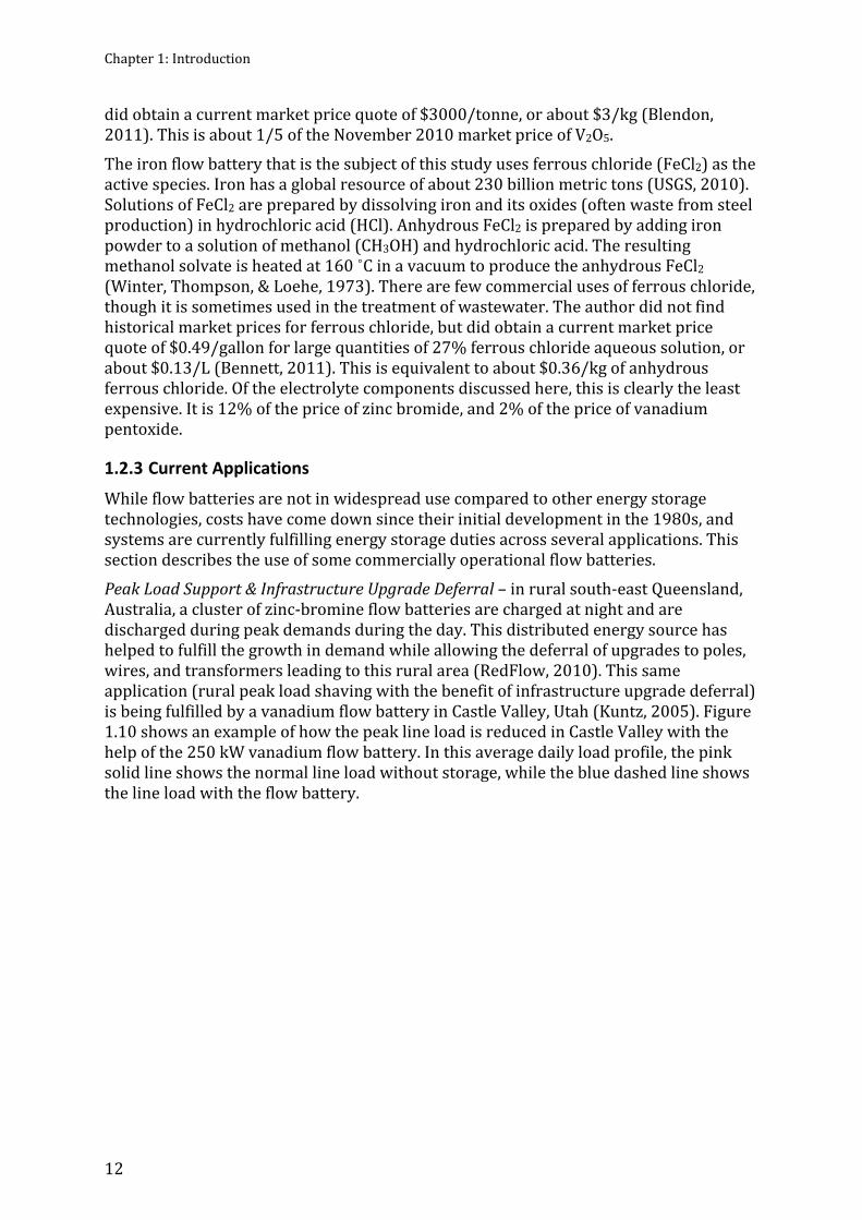
did obtain a current market price quote of $3000/tonne, or about $3/kg (Blendon, 2011). This is about 1/5 of the November 2010 market price of V2O5. The iron flow battery that is the subject of this study uses ferrous chloride (FeCl2) as the active species. Iron has a global resource of about 230 billion metric tons (USGS, 2010). Solutions of FeCl2 are prepared by dissolving iron and its oxides (often waste from steel production) in hydrochloric acid (HCl). Anhydrous FeCl2 is prepared by adding iron powder to a solution of methanol (CH3OH) and hydrochloric acid. The resulting methanol solvate is heated at 160 ˚C in a vacuum to produce the anhydrous FeCl2 (Winter, Thompson, & Loehe, 1973). There are few commercial uses of ferrous chloride, though it is sometimes used in the treatment of wastewater. The author did not find historical market prices for ferrous chloride, but did obtain a current market price quote of $0.49/gallon for large quantities of 27% ferrous chloride aqueous solution, or about $0.13/L (Bennett, 2011). This is equivalent to about $0.36/kg of anhydrous ferrous chloride. Of the electrolyte components discussed here, this is clearly the least expensive. It is 12% of the price of zinc bromide, and 2% of the price of vanadium pentoxide. 1.2.3 Current Applications While flow batteries are not in widespread use compared to other energy storage technologies, costs have come down since their initial development in the 1980s, and systems are currently fulfilling energy storage duties across several applications. This section describes the use of some commercially operational flow batteries. Peak Load Support & Infrastructure Upgrade Deferral – in rural south-east Queensland, Australia, a cluster of zinc-bromine flow batteries are charged at night and are discharged during peak demands during the day. This distributed energy source has helped to fulfill the growth in demand while allowing the deferral of upgrades to poles, wires, and transformers leading to this rural area (RedFlow, 2010). This same application (rural peak load shaving with the benefit of infrastructure upgrade deferral) is being fulfilled by a vanadium flow battery in Castle Valley, Utah (Kuntz, 2005). Figure 1.10 shows an example of how the peak line load is reduced in Castle Valley with the help of the 250 kW vanadium flow battery. In this average daily load profile, the pink solid line shows the normal line load without storage, while the blue dashed line shows the line load with the flow battery.
James Mellentine
13
Figure 1.10 – The daily load profile of the rural feeder line in Castle Valley Utah. The pink solid line shows the
normal line load without energy storage. The blue dashed line shows the line load with the vanadium flow battery installed – it shaves the peak to be within the capacity limit of the electricity lines, thus allowing for
continued demand increase while deferring expensive infrastructure upgrades (Kuntz, 2005).
Backup Power and Cost Reduction – Pualani Manor is a mid-rise apartment building in Honolulu, Hawaii that is using a zinc bromine flow battery as a backup electricity source for their elevator as well as a reduction of electricity costs via utility incentives. Electricity is very expensive in Hawaii, and the utility pays a monetary incentive for renewable energy generation during peak loads, so in addition to serving as backup power, the building discharges the battery daily during peak loads to maximize overall energy savings and its return on investment (ZBB Energy, 2010). Wind Energy Grid Integration – On Hokkaido Island, Japan, a 4 MW/6 MWh vanadium flow battery system is paired to a 32 MW wind farm. The battery helps match power supply and demand curves under varying weather conditions, significantly increasing the output (and profit) of the wind farm operator (Prudent Energy). Uninterruptible Power Supply (UPS) – In India, small 2 kW/8 kWh iron chromium flow batteries are serving as backup power supplies to cell phone towers. In developing countries like India, where power supplies are not as reliable, this is an important function to keep cell phone networks functioning (NASA, 2010). This concept can be applied to other uses as well, such as traffic lights, hospitals, or critical industrial processes. 1.3 Thesis Objective It has been shown in a previous study that an iron hybrid flow battery is feasible, with 50% energy efficiency and 50 mW/cm2 power density achieved (Hruska & Savinell, 1981). There have recently been research efforts to identify new electrolyte ligands which could improve the overall performance of the battery (Wainwright, 2010).

Chapter 1: Introduction
14
The first objective of this thesis was to collaborate with experts at InnoVentures Incorporated to develop an appropriate stack design based on estimated performance characteristics of an iron flow battery and power & energy capacity requirements. InnoVentures is a company that designs and manufactures fuel cell and flow battery equipment, and they often collaborate with researchers at CWRU. The designed system component costs were also estimated in collaboration with InnoVentures. Some component price estimates were also received from Brenntag Group, Den Hartog Industries, and Daramic. The most likely, pessimistic, and optimistic prices were obtained for the following battery components: • Activated felt • Bipolar plates • Flow frames • Separator • Electrolyte material • Electrolyte preparation • Tanks • Pumps • Control/Management system A total estimated system cost was obtained for the proposed stack design based on the component price estimates. This cost was used to calculate the system cost on a per-kW and per-kWh basis. These costs were then compared to other flow battery chemistries such as zinc-bromine and vanadium as available in the literature. A sensitivity analysis was performed on the individual components listed above to determine which have the greatest impact on the stack price. The components shown to be the most sensitive were used in a Monte Carlo simulation to provide a more robust indication of the estimated cost of the designed stack. A sensitivity analysis was also performed on the estimated performance characteristics of the battery, providing an indication of how much the cost of the system can be lowered based on targeted performance increases. The second objective of this thesis was to match the designed to a specific application and to analyze performance. Chapter 4 outlines the performance of a scaled-up battery in an area regulation application. Using area regulation data from the California Independent Service Operator (CAISO), an analysis of the battery’s performance through a one-year period was conducted. The battery’s availability to provide service, the state of charge in each hour of the year, and the battery’s estimated revenue and costs during the operations were determined. The final objective of this thesis was to characterize the performance of a single-cell iron hybrid flow battery in the laboratory using a suggested electrolyte chemistry that was anticipated to result in performance improvements. The chlorides of iron were used in this study, since they have been shown to exhibit low resistivity in the concentration range of 0.8-3.9 M while pH changes are moderate within the same concentration range (Hruska & Savinell, 1981). The same referenced study has also shown that adding ammonium chloride (NH4Cl) to aqueous FeCl2 further reduces the resistivity of the electrolyte while improving plating characteristics. Based on the guidance of a faculty researcher, boric acid (H3BO3) was also added to the electrolyte as a ligand to hinder hydrogen evolution on charge (which lowers energy efficiency and affects electrolyte pH). Initial experiments with the microporous membrane used an electrolyte solution of 0.65 M FeCl2 and 1 M NH4Cl on the negative side, and an electrolyte solution of 0.65 M

James Mellentine
15
FeCl2, 1 M NH4Cl, and 1 M H3BO3. This was eventually changed such that the 1 M H3BO3 was on both sides of the cell. Later experiments with the Nafion membrane used an electrolyte solution of 1 M FeCl2, 1 M NaCl, and 1 M H3BO3. The NaCl replaced the NH4Cl as the supporting electrolyte due to the latter’s apparent incompatibility with Nafion. A 50 cm2 single cell test station was assembled in the laboratory at Case Western Reserve University (CWRU). This station, with the above electrolyte, was used for this study. The test station is fully automated for charge and discharge functions. The station is connected to a computer running LabVIEW software, with a virtual interface (VI) and control system developed by other researchers in the lab (National Instruments, 2010). This commonly-used laboratory software displayed and recorded measurements. The data collected from this lab setup was used to characterize the performance of the cell. Later in this report, the performance data is compared to other flow battery chemistries such as zinc-bromine and vanadium. The data was also compared to the estimated performance data used in the economic model above, highlighting areas that need improvement. In summary, the iron hybrid flow battery has the potential to be a lower cost large-scale energy storage solution. The objectives of this thesis are to develop an iron flow battery system cost using estimated performance characteristics, perform an analysis of the flow battery in a hypothetical application, and document preliminary performance data of a single-cell iron flow battery in the laboratory.

Chapter 1: Introduction
16

James Mellentine
17
Chapter 2: Literature Review Flow battery technology was originally developed in the mid-1970s (Thaller, 1976). Since then, research has focus on various electrolyte chemistries. Since flow battery systems are generally characterized by relatively low energy density compared with other energy storage technologies, stationary uses have been the primary focus for practical application. While not in widespread use, zinc-bromine hybrid flow batteries are the most commonly used type of flow battery in the United States (Roselund, 2010). Vanadium redox flow battery chemistry has been the subject of much recent flow battery research. The performance of an all-iron hybrid flow battery has previously been investigated, but no further research and development has occurred (Hruska & Savinell, 1981). In 2006, UK and Spanish researchers published a widely-cited review of current redox flow battery technology, and this literature review will not attempt to overlap that work (Ponce de Leon, Frias-Ferrer, Gonzalez-Garcia, Szanto, & Walsh, 2006). Instead, this chapter will focus on research that has been published since then. The areas of published research can be divided into primary areas of electrolyte improvements, membrane improvements, and electrode improvements. This review will focus on the various electrolytes that have been recently studied. The chapter concludes with a description of how the iron hybrid flow battery that is the subject of this study contributes to the field of flow battery research. 2.1 Recent Electrolyte Research Flow batteries in the traditional sense have all electroactive species dissolved in the electrolyte, whereas hybrid flow batteries have at least one species that can exist in a solid state (usually deposited or plated onto an electrode). The primary difference in these flow battery types besides the aqueous vs. solid distinction is that the hybrid flow battery energy capacity is limited by the amount of metal that can be plated onto the electrode. 2.1.1 Vanadium-based Electrolytes Development of vanadium redox flow batteries began in 1985 at the University of New South Wales (UNSW) in Australia, with a patent granted in 1986 (UNSW, 2010). These batteries generally have electrolyte composed of vanadyl sulfate (VOSO4) – which is derived from vanadium pentoxide (V2O5) – dissolved in sulfuric acid (H2SO4) on both sides of the cell. In an ambient temperature range, VOSO4 concentrations of up to 2M can be achieved. From this reaction, two primary cations exist in solution: VO2+ and V3+. When the battery is charged, the VO2+ ions on the positive side lose an electron and form VO2+. Meanwhile, the V3+ ions on the negative side gain those electrons and are reduced to V2+. To preserve electroneutrality, hydronium ions (H3O+) travel across the membrane separator in the same direction as the electrons. A summary of these reactions are presented below:

Chapter 2: Literature Review
18
Positive side charge: VO2+ + H2O → VO2+ + 2H++2e- Negative side charge: V3+ + e- → V2+ Positive side discharge: VO2++2H++2e- → VO2++H2O Negative side discharge: V2+ → V3+ + e- The standard cell potential of the discharge reaction is 1.26 V @ 25 ˚C, but in actual cell conditions, the open-circuit voltage is around 1.6 V at 100% state of charge (SOC) and around 1.4 V at 50% SOC – thus 1.4V is the generally assumed nominal voltage for vanadium redox batteries (EPRI, 2007). Specific energies of up to 35 Wh/kg can be achieved with vanadium redox batteries according to UNSW (Skyllas-Kazacos, 2010). A representative from the former VRB Systems, a now-bankrupt manufacturer of vanadium redox batteries, claims usable energy densities of 20-30 Wh/L (about 31-47 Wh/kg assuming 2 M vanadyl sulfate and 2.5 M sulfuric acid concentrations) (EPRI, 2007). Therefore, a 20 kWh system (a similar energy capacity as the iron hybrid flow battery in this paper) would require about 660-1000 liters of electrolyte, evenly split between a positive and negative tank. Vanadium redox batteries achieve a power density of approximately 65 mW/cm2 while operating at a current density of 50 mA/cm2. Operational current densities above 100 mA/cm2 are not practical (EPRI, 2007). Round-trip DC-to-DC energy efficiencies of over 80% have been achieved in production systems (Skyllas-Kazacos, 2010). One area of research for the vanadium battery (and a common goal for most battery technologies) is focused on increasing the energy density. Most commercial vanadium systems run at or below a vanadium concentration of 2 M due to solubility limits in sulfuric acid solutions. Increasing the solubility of vanadium ions in the electrolyte will effectively increase the energy density of the system. An example of this research is a study from UNSW that shows a stable concentration of 4 M vanadyl sulfate can be achieved in a 3 M sulfuric acid solution with the addition of sodium hexametaphosphate(Skyllas-Kazacos, Peng, & Cheng, 1999). The same research group has also developed a so-called “Generation 2” vanadium redox battery that rely on a different electrolyte composition with different redox couples – vanadium trichloride in hydrochloric acid solution on the negative side and sodium bromide in hydrochloric acid solution on the positive side – that also allows vanadium concentrations up to 4 M due to the higher solubility of hydrochloric acid (Skyllas-Kazacos, 2003). UNSW has demonstrated a Generation 2 vanadium bromide cell using a 3 M vanadium bromide electrolyte with the successful prevention of bromine vapor formation using complexing agents. Current studies of this cell have about twice the energy density of the original vanadium redox flow battery (Skyllas-Kazacos, Kazacos, Poon, & Verseema, 2010). Though the vanadium electrolytes have been researched extensively, there has been little information on the thermodynamic properties and behavior of the electrolyte. This information could be helpful to better understand the reactions that occur within the cell and to serve as a basis for incremental performance improvements. A series of research efforts in China have aimed to fill this gap in knowledge by experimentally providing the data for molar enthalpies and entropies of vanadium electrolyte solutions. Ye et al have determined the low-temperature heat capacities of VOSO4•2.63H2O for a range of temperatures, along with calculating the molar enthalpy and entropy of

James Mellentine
19
dehydration (Ye, Liu, Di, Yan, Zeng, & Yang, 2010). Participants of the same group have also estimated the standard molar enthalpies of vanadyl sulfate in both water and sulfuric acid, with data indicating that the energy state of VOSO4 in sulfuric acid is higher than in water (Ye, Xue, Liu, Xu, Yan, & Yang, 2010). A research group in the UK has focused their research efforts toward modeling various aspects of the vanadium redox flow battery system. First, a two-dimensional model was developed using conservation of mass, charge, and momentum principles. The model was validated against experimental data found to be in good agreement. It could be used to study various performance effects from variations in concentration, flow rate, and electrode properties (Shah, Watt-Smith, & Walsh, 2008). In another study, the model was used to show how operating temperature affects performance. It found that without including heat dissipation techniques, temperatures could quickly rise to harmful levels, especially as loads increase. The model also found that localized regions of high temperature within the cell can develop due to non-uniform reactivity, which can be avoided with an increased electrolyte flow rate (Al-Fetlawi, Shah, & Walsh, 2009). The same research group has also developed models for the gas evolution process in vanadium redox electrolytes. Understanding the mechanisms and behavior of gas evolution could help decrease the occurrence of the behavior and thus increase the efficiency of batteries. Again, conservation equations of mass, charge, and momentum were used to develop a model for hydrogen evolution on the negative side of the vanadium redox battery. The resulting model was compared to experimental data and shown to be in good agreement. One result from this data was the finding that the presence of bubbles in the cell does not have as much effect on performance as the loss of current required to evolve the hydrogen. Another finding was that an increased flow rate at an increased current density could be used to minimize the increase in gas volume within the cell (Shah, Al-Fetlawi, & Walsh, Dynamic modelling of hydrogen evolution effects in the all-vanadium redox flow battery, 2010). A similar model for oxygen evolution on the positive side of the cell was created, again with good agreement with experimental data. The model shows a range oxygen volume fraction range of 2%-13%, resulting in a drop in charge efficiency of 5%-10%. The volume fraction decreases with increasing flow rate. Volume fraction is also highly dependent on bubble diameter, with a larger bubble diameter resulting in a decreased volume fraction (due to greater buoyancy). The evolution of oxygen was also shown to depend highly on temperature in a positively correlated relationship. The cell efficiency is significantly decreased with an increase in cell temperature (Al-Fetlawi, Shah, & Walsh, Modelling the effects of oxygen evolution in the all-vanadium redox flow battery, 2010). A research group at the Pacific Northwest National Laboratory (PNNL) has used nuclear magnetic resonance spectroscopy to observe the structure of vanadium (IV) species. They have shown that the vanadyl ion is stable in vanadium concentrations from 0.1 M to 3 M within a large temperature range. The vanadyl ion is also surrounded by sulfate ions in solution. Further, the vanadyl ion becomes less mobile as vanadium or sulfate concentration increases. The spectroscopy results also show that an increase in sulfate concentration increases the probability of water exchange (Vijayakumar, et al., 2010). Other research with non-aqueous vanadium electrolytes has been conducted. A collaborative study between US and China universities has shown preliminary voltammetric data for a cell that used an electrolyte on both sides of cell composed of
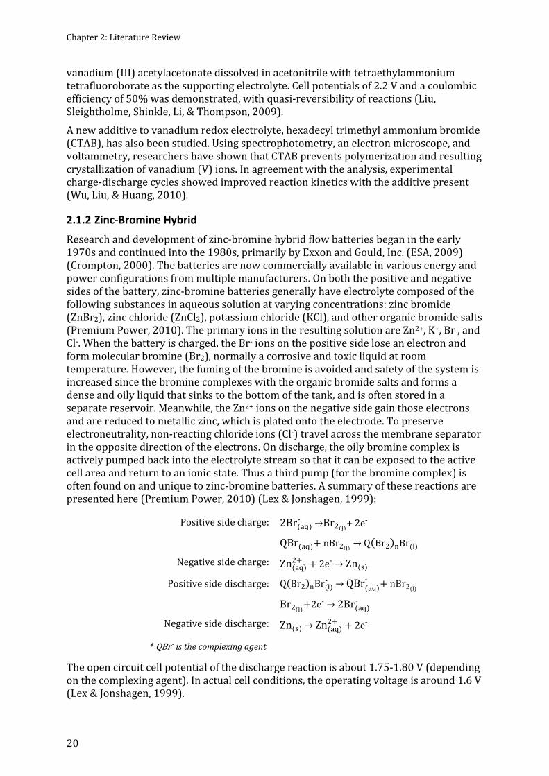
Chapter 2: Literature Review
20
vanadium (III) acetylacetonate dissolved in acetonitrile with tetraethylammonium tetrafluoroborate as the supporting electrolyte. Cell potentials of 2.2 V and a coulombic efficiency of 50% was demonstrated, with quasi-reversibility of reactions (Liu, Sleightholme, Shinkle, Li, & Thompson, 2009). A new additive to vanadium redox electrolyte, hexadecyl trimethyl ammonium bromide (CTAB), has also been studied. Using spectrophotometry, an electron microscope, and voltammetry, researchers have shown that CTAB prevents polymerization and resulting crystallization of vanadium (V) ions. In agreement with the analysis, experimental charge-discharge cycles showed improved reaction kinetics with the additive present (Wu, Liu, & Huang, 2010). 2.1.2 Zinc-Bromine Hybrid Research and development of zinc-bromine hybrid flow batteries began in the early 1970s and continued into the 1980s, primarily by Exxon and Gould, Inc. (ESA, 2009) (Crompton, 2000). The batteries are now commercially available in various energy and power configurations from multiple manufacturers. On both the positive and negative sides of the battery, zinc-bromine batteries generally have electrolyte composed of the following substances in aqueous solution at varying concentrations: zinc bromide (ZnBr2), zinc chloride (ZnCl2), potassium chloride (KCl), and other organic bromide salts (Premium Power, 2010). The primary ions in the resulting solution are Zn2+, K+, Br-, and Cl-. When the battery is charged, the Br- ions on the positive side lose an electron and form molecular bromine (Br2), normally a corrosive and toxic liquid at room temperature. However, the fuming of the bromine is avoided and safety of the system is increased since the bromine complexes with the organic bromide salts and forms a dense and oily liquid that sinks to the bottom of the tank, and is often stored in a separate reservoir. Meanwhile, the Zn2+ ions on the negative side gain those electrons and are reduced to metallic zinc, which is plated onto the electrode. To preserve electroneutrality, non-reacting chloride ions (Cl-) travel across the membrane separator in the opposite direction of the electrons. On discharge, the oily bromine complex is actively pumped back into the electrolyte stream so that it can be exposed to the active cell area and return to an ionic state. Thus a third pump (for the bromine complex) is often found on and unique to zinc-bromine batteries. A summary of these reactions are presented here (Premium Power, 2010) (Lex & Jonshagen, 1999): Positive side charge: 2Br(aq)- →Br2(l)+ 2e- QBr(aq)- + nBr2(l) → Q(Br2)nBr(l)- Negative side charge: Zn(aq)2+ + 2e- → Zn(s) Positive side discharge: Q(Br2)nBr(l)- → QBr(aq)- + nBr2(l) Br2(l)+2e- → 2Br(aq)- Negative side discharge: Zn(s) → Zn(aq)2+ + 2e-
* QBr- is the complexing agent The open circuit cell potential of the discharge reaction is about 1.75-1.80 V (depending on the complexing agent). In actual cell conditions, the operating voltage is around 1.6 V (Lex & Jonshagen, 1999).

James Mellentine
21
Specific energies of 75-85 Wh/kg are claimed by ZBB Energy, a US-based manufacturer of zinc-bromine battery systems (ZBB Energy, 2010). Practical energy densities of up to 50 Wh/L can be achieved (Crompton, 2000). Therefore, a 20 kWh system (a similar energy capacity as the iron hybrid flow battery design proposed in this study) would require about 400 liters of electrolyte, evenly split between a positive and negative tank. Zinc-bromine batteries achieve a power density of approximately 60 mW/cm2 while operating at a current density of 37.5 mA/cm2 (Leo, 1989). Round-trip DC-to-DC energy efficiency of about 75% is typical (ESA, 2009). Since Ponce de Leon’s technology review in 2006, very little published research has focused on the zinc-bromine flow battery. However, some research has focused on the deposition of zinc and with other zinc-based electrolytes. A new zinc-air flow battery has been proposed by researchers in China. A single liquid electrode flows through a cell that has a negative electrode on one side (where zinc is plated/stripped) and an oxygen composite electrode on the other side, which has a dual-layer that is exposed to the atmosphere. When atmospheric oxygen comes into contact with the nano-structured nickel hydroxide membrane, nickel oxyhydroxide and water are formed. On the higher-temperature liquid side of the membrane, the nickel oxyhydroxide reduces back to nickel hydroxide and oxygen gas is formed. At the same time, zinc hydroxide ion accepts electrons, forming metallic zinc onto the electrode, and water in the solution. 150 charge-discharge cycles at a current density of 20 mA/cm2 and a plating density of 50 mA-hr/cm2 showed an average discharge voltage of 1.32 V and an average energy efficiency of 72.2% (Pan, et al., 2009). A zinc-nickel flow battery with similar chemistry of the zinc-air battery has been demonstrated by the same group. The single electrolyte is concentrated zinc oxide dissolved in potassium hydroxide or sodium hydroxide solution. The electrolyte is pumped through a membrane-less cell with a positive electrode composed of nickel hydroxide and a negative electrode composed of an inert metal substrate. On the positive side, nickel hydroxide is oxidized to nickel oxyhydroxide while zinc metal plates onto the positive electrode. 1000 cycles were conducted with a current density of 10 mA/cm2 and plating density of 20 mA-hr/cm2, resulting in an average energy efficiency of 86% (Cheng, Zhang, Yang, Wen, Cao, & Wang, 2007). When zinc deposits onto an electrode, it can form an undesirable spongy structure. Researchers have studied additives (lead oxide and sodium tungstate) that eliminated or reduced the formation of the spongy structure. Optimal concentrations of 0.6M Na2WO4 or 10-4 to 10-3 M PbO were determined and experimentally tested in a zinc-air flow battery, with 60% energy efficiency achieved (Wen Y.-h. , Cheng, Zhang, Yan, & Yang, 2009). 2.1.3 Other electrolyte research Several research groups are also focused on developing new and novel electrolyte chemistries for flow batteries. At the University of Manchester, researchers focused on finding electrolytes which could be the same on both sides to avoid crossover problems and which offer fast kinetics and good solubility. Ruthenium acetylacetonate in acetonitrile and tris(2,2’-bipyridine) iron (II) perchlorate in acetonitrile were briefly tested and reported. In

Chapter 2: Literature Review
22
limited charge-discharge tests, the former achieved an energy efficiency of 74%, while the latter achieved only 6% (Chakrabarti, Dryfe, & Roberts, 2007). Another team at the University of Manchester teamed up with Regenesys Technologies to create a one-dimensional model for a bromide-polysulfide redox flow battery. Using the Butler-Volmer equation and mass transfer principles, they were able to create a model that predicted concentration and current variation within the electrodes, as well as predict energy efficiency and power density. A pilot-scale stack was cycled 17 times at current densities of 40 mA/cm2 and 60 mA/cm2 to make sure the actual data agreed with the model. The model was useful in finding that overpotentials at the bromide electrode were limiting the performance, and that electrolyte conditions were very sensitive to self-discharge and electro-osmotic forces (Scamman, Reade, & Roberts, Numerical modelling of a bromide-polysulphide redox flow battery, Part 1: Modelling approach and validation for a pilot-scale system, 2009). The same model was then combined with a cost model to predict the technical and economic performance of 15 MW/120 MWh storage plant. The model predicted the system would have an energy efficiency of 64% and operate at a net loss (Scamman, Reade, & Roberts, 2009). A research group at the University of Southampton has continued to advance the technology of the lead-acid flow battery that they previously proposed. This flow battery is a single-flow membrane-less battery that, during charge, deposits lead dioxide onto the positive electrode and lead onto the negative electrode. One focus of research was to find additives to improve the quality of deposits of lead onto the negative electrode. The researchers found that a good additive was 5 mM of hexadecyltrimethylammonium cation to 1.2 M of lead dissolved in methanesulfonic acid (Pletcher, Zhou, Kear, Low, Walsh, & Wills, A novel flow battery—A lead-acid battery based on an electrolyte with soluble lead (II). V: Studies of the lead negative electrode, 2008). Regarding the deposition of lead oxide onto the negative electrode, the limiting current density was determined to be about 100 mA/cm2, above with internal stress fractures the deposited lead oxide. However, other limiting factors such as oxygen evolution and overpotential require a lower current density, so the deposit of lead oxide would not be an issue for their recommended operational range of 20 mA/cm2 to 80 mA/cm2 (Pletcher, Zhou, Kear, Low, Walsh, & Wills, 2008). Possible failure modes of the battery have been identified as lead dendrites or lead dioxide creep that cause electrical shorts, or lead dioxide sludge that could clog the plenum inlet (Wills, Collins, Stratton-Campbell, Low, Pletcher, & Walsh, 2010). Further detailed studies on lead dioxide reduction revealed that operating the battery at less than 0.3 M lead is not recommended (Li, Pletcher, & Walsh, 2009). Due to a coulombic efficiency less than 100%, some deposits remained on the electrodes after each cycle. The leftover deposit gradually built up and over the course of 20 cycles, the performance was demonstrated to significantly degrade (Collins, et al., 2010). The periodic addition of hydrogen peroxide into the electrolyte was shown to completely re-dissolve the built-up deposits and restore the performance of the battery (Collins, et al., 2010). The latest published work on the battery is the development of a model for the battery which incorporates charge and mass transport principles along with surface electrode reactions. The model predictions were compared to experimental data and found to be in good agreement. Further enhancements to the model are stated to be underway (Shah, Li, Wills, & Walsh, 2010). A similar single-flow battery has been developed by a collaboration of Universities in China. The battery has a concentration of 0.6 M copper sulfate in 2 M sulfuric acid. On

James Mellentine
23
charge, lead dioxide is deposited onto the positive electrode, and copper is deposited onto the negative electrode. Good performance has been demonstrated on a 24 cm2 cell through 450 charge-discharge cycles using a current density of 40 mA/cm2. The discharge voltage is 1.29 V, with an average energy efficiency of 83% reported (Pan, Sun, Cheng, Wen, Yang, & Wan, 2008). Researchers at the University of Michigan and Tianjin University have investigated the possibility of using a non-aqueous chromium acetylacetonate electrolyte. They prepared a solution containing 0.05 M chromium acetylacetonate (Cr(acac)3) and 0.5 M tetrafluoroborate in acetonitrile. Using cyclic voltammetry, the researchers demonstrated that the chromium complex can be both oxidized +1 and +2 states and reduced to -1 and -2 states. The researchers estimate the cell potential at 3.4 V. However, initial energy efficiencies were quite low at 22% (Liu, Shinkle, Li, Monroe, Thompson, & Sleightholme, 2010). Research has also been demonstrated for organic compounds, with the intent of bringing down costs by avoiding metal-based electrolytes. Tiron, an organic compound that has typically been used as a chelator or indicator in chemical experiments, was demonstrated to be suitable as a flow battery electrolyte. An electrolyte solution containing 0.05 M tiron in 1 M potassium chloride (aqueous) was tested using cyclic voltammetry, using a range of adjusted pH. It was found that the reactions of tiron are best below a pH of 4, with reactions showing quasi-reversibility and fast electrode kinetics. The electrolyte was also pumped through a flow battery cell with a current density of 10 mA/cm2 and Nafion membrane. An average energy efficiency of 82% was demonstrated (Xu Y. , Wen, Cheng, Cao, & Yang, 2010). The same research group has investigated a single-flow battery with an organic compound as the positive electrode and cadmium as the electrolyte. The single-flow cell used a copper negative electrode, onto with cadmium plates during charge. The positive electrode was made of chloranil mixed with carbon black and a Teflon binder. The electrolyte was 0.5 M cadmium sulfate and 1 M ammonium sulfate in 0.5 M sulfuric acid. On charge, the chloranil in the positive electrode oxidizes to chloranilic acid. The small experimental battery was cycled 100 times at 10 mA/cm2, showing an average energy efficiency of 82% (Xu Y. , Wen, Cheng, Cao, & Yang, 2009). A study from South Africa has found that pentetic acid is an effective ligand for a cerium (IV)-based electrolyte. Using cyclic voltammetry and platinum electrodes, it was demonstrated that the electron transfer rate of the cerium (IV) – pentetic acid complex is faster than uncomplexed cerium (IV), with k values between 1.6-3.1 × 10⁻⁴ cm/s. The research suggests that this electrolyte could be used on the positive side of a redox flow battery to provide high voltaic efficiency (Modiba & Crouch, 2008). While an all-uranium redox flow battery has previously been demonstrated, little recent published research moves the technology forward, likely due to the safety hazards of having a radioactive electrolyte. However, a Japan-based research group has investigated the use of ligands in uranium redox reactions. Using tetraketones complexed with uranium, the researchers showed that electron transfer between uranium (VI)/uranium (V) is significantly improved, while the reversibility of the uranium (IV)/uranium (III) reaction is also improved (Yamamura, et al., 2007). A novel concept of a redox flow battery combined with commercial production of organic material has also been proposed. Figure 2.1 shows a diagram of the proposed bifunctional redox flow battery. Essentially, a traditional redox couple electrolyte

Chapter 2: Literature Review
24
(vanadium in this case)is pumped through two cells. On charge, organic materials enter the cell and exit as some generic organic product, while charge is stored on the other side of the cell in the redox couple. On discharge, the redox couple is exposed to oxygen in the second cell to provide energy. In the study, organic electrolyte was 1 M glyoxal in 3 M HCl, while the redox electrolyte was 2 M vanadium (III) in 3 M sulfuric acid. Some enhancements were made to a Nafion membrane to prevent the crossover of vanadium into the organic electrolyte. The charge voltage was demonstrated to be around 2.3 V, with low current efficiencies due to the synthesis of organic product. The battery was discharged for 20 hours at 20 mA/cm2, showing that the concept is feasible even though more research is required to improve performance (Wen Y. H., Cheng, Ma, & Yang, 2008).
Figure 2.1 – Bifunctional redox flow battery concept (Wen Y. H., Cheng, Ma, & Yang, 2008).
2.2 Thesis Contribution An iron hybrid flow battery was originally proposed and demonstrated by the thesis supervisor in 1980 (Hruska & Savinell, 1981). In the referenced study, the battery was charged and discharged 100 times at a current density of 60 mA/cm2, through a 100 cm2 cell. The battery was demonstrated to have a maximum energy efficiency of 50%, with a power density of 50 mW/cm2. Since then, no published research has been found that furthered the research. The proposed battery uses a ferrous chloride salt in aqueous solution with ammonium chloride as the supporting electrolyte. On the negative side of the battery, ferrous ions are reduced during charge, plating as iron metal onto a graphite electrode. On the positive side of the battery, ferrous ions are oxidized to ferric ions during charge, remaining in solution. These reactions are the opposite upon discharge. To preserve electroneutrality, chloride ions (Cl-) travel across the microporous membrane separator in the opposite direction as the electrons. A summary of the charge and discharge reactions along with standard potentials are presented here: EO Positive side charge: Fe2+ → Fe3++e- -0.77 V Negative side charge: Fe2+ +2e- → Fe(s) +0.41 V Net charge reaction: 2Fe2+ + e- → Fe3+ + Fe(s) -1.18 V Positive side discharge: Fe3++e- → Fe2+ +0.77 V Negative side discharge: Fe(s) → Fe2+ + 2e- -0.41 V Net discharge reaction: Fe3+ + Fe(s) → 2Fe2+ + e- +1.18 V

James Mellentine
25
It is important to note that the open circuit voltage of a flow battery changes according to the state of charge due to changes in reactant concentration. For the iron hybrid flow battery that is the subject of this study, the open circuit potential can be expressed in terms of the Nernst equation as follows: = − [ 2+] [ 2+]0.5[ 3+] Where: VOC = open circuit voltage of the cell VO = standard cell potential R = universal gas constant T = cell temperature F = Faraday constant [Fe2+]P = concentration of ferrous ion in the positive half-cell [Fe3+]P = concentration of ferric ion in the positive half-cell [Fe2+]N = concentration of ferrous ion in the negative half-cell The change in open circuit voltage can be graphed as a function of state of charge if the concentration values are expressed in terms of the state of charge. The state of charge (SOC) can be expressed as the concentration of ferric ions divided by the concentration of ferrous ions at a 0% SOC (referring to the positive side reaction): = 0 Rearranging the equation, the concentration of ferric ion on the positive side is: [ 3+] = × [ 2+]0 Next we consider that the ferrous ion concentration is directly proportional to the starting ferrous ion concentration at 0% SOC and the state of discharge (1 – SOC): [ 2+] = [ 2+]0(1 − ) Similarly on the negative side of the cell, the ferrous ion concentration can be expressed in terms of state of charge: 1 − = 0 [ 2+] = [ 2+]0 (1 − ) Now, all of the solved concentration values are plugged into the Nernst equation above to get the open circuit voltage in terms of SOC. = − ([ 2+]0 )0.5(1 − )1.5 A graph of the open circuit voltage versus state of charge is shown in Figure 2.2.

Chapter 2: Literature Review
26
Figure 2.2 – The open circuit voltage of the iron hybrid flow battery versus state of charge. The promise of an iron hybrid flow battery is not necessarily in superior efficiency or energy density compared to other flow battery technologies, but in its potential to significantly lower the cost of energy storage. An iron-based electrolyte that isn’t as efficient as a vanadium system might still outperform it economically. In an effort to revive research efforts surrounding the concept, another research faculty member at CWRU has recently studied various ligands that may have potential to improve the performance of the iron hybrid flow battery (Wainwright, 2010). One of the more promising ligands, boric acid, was chosen for further investigation in this study in order to characterize its performance in repeated cycles in a laboratory cell. The iron flow battery in this study has an electrolyte composed of 1M ferrous chloride (FeCl2), 1M sodium chloride (NaCl), and 0.7 M – 1 M boric acid (H3BO3) dissolved in de-ionized water. In parallel to the laboratory investigations, some initial performance assumptions were made in order to develop a cost model for such a battery. A demonstrated low cost to manufacture such a device could spur additional interest and result in research efforts to improve the technology. The cost model could also help a potential manufacturer to decide if there is a possible business case and identify components that could help drive costs lower. The results of this study will contribute to flow battery research by demonstrating the performance of a little-studied chemistry using a new ligand. It will also demonstrate a realistic cost of production of such a device, along with its performance in a hypothetical area regulation application.

James Mellentine
27
Chapter 3: Cost Analysis of Iron Hybrid Flow Battery A flow battery electrolyte composed of inexpensive chemicals could decrease the cost of the flow battery system, as shown previously in this paper. This chapter aims to estimate the cost of a flow battery system using an iron-based electrolyte. From this estimate, cost on a per-kW and per-kWh was calculated and compared with other technologies. The system cost was completed by considering the costs of its individual components. To determine the size and design of the individual components, assumed performance characteristics of the battery were used to calculate other system characteristics. Optimistic, most-likely, and pessimistic price estimates were provided by InnoVentures and other companies. A three-point analysis was then conducted using a triangular distribution to determine an “expected” system cost. Sensitivity analyses were also performed to determine the primary drivers of system cost. System costs were also compared to other energy storage technologies. 3.1 Design Approach and Results The iron hybrid flow battery system design was based on the following assumed system and performance characteristics. Table 3.1 – Assumed system and performance characteristics of an iron hybrid flow battery system. Subsequent system design and performance characteristics were calculated from these assumptions.
System/Performance Characteristic Value System/Performance
Characteristic Value
Power capacity 10 kW Annual production 1000 units Current density 50 mA/cm2 Cell thickness 0.318 cm Nominal cell voltage 1.2 V Cell height/width 49.21 cm/ 60.96 cm Maximum plating density 100 mA-hr/cm2 Electrode area 3000 cm2 Coulombic efficiency 85% Parasitic loss 6% Voltaic efficiency 65% Inverter loss 6%
Electrolyte composition 1M FeCl2; 1M H3BO3; 1M NH4Cl in de-ionized water Operating Temperature 40 ˚C The current density, nominal cell voltage, maximum plating density, and efficiency values were chosen as reasonable estimates based on the thesis supervisor’s previous study, as well as parallel experimental results in the lab that will be discussed later (Hruska & Savinell, 1981). The electrolyte composition was suggested by other research faculty (Wainwright, 2010). The operating temperature was selected to be sufficiently high enough to keep 1 M boric acid in solution. At 40 ˚C, boric acid has a maximum solubility of 1.4 M (Incide Technologies, 2006). The power capacity, electrode area, cell thickness, and annual production values were suggested by InnoVentures. The parasitic

Chapter 3: Cost Analysis of Iron Hybrid Flow Battery
28
and inverter loss estimates were based on values used in other studies (Witmer, 2008) (Chahwan, Abbey, & Joos, 2007). The first performance characteristic calculated from these assumed values was power density. The following formula shows the power density calculation. This assumes that the voltaic efficiency is symmetrical for charge and discharge, thus the voltaic efficiency for discharge only is the square root of the overall voltaic efficiency. = × × = 50 × 1.2 × √. 65 = The electrode area of 3000 cm2 was chosen because this is the largest electrode area that InnoVentures currently manufactures, so costs are well known. Based on the power density and the electrode area, the nominal power per cell were calculated as follows: − = × − = 48 × 3000 = . / Next, the number of cells in the stack can be calculated based on the stack power capacity, parasitic and inverter losses, and power per-cell. = × (1 + + ) − = 10 × (1 + 0.06 + 0.06)0.1451 / = The number of cells was rounded up to the next whole number since there are not fractions of cells in the design. Once the number of cells was known, I referenced a NASA study to estimate the shunt current losses in the system. The study specifically developed a model to calculate shunt current losses in electrochemical stacks using a similar electrolyte. A stack of 80 cells, for example, would have a power loss of around 10 W, while a stack of 120 cells would have a power loss of around 20 W (Prokopius, 1976). Since the number of cells is 75, a shunt loss of 10 W was chosen as a conservative estimate. Once determined, this small shunt loss was then incorporated into the number-of-cells calculation above (with the parasitic and inverter losses) to ensure that the system power was capable of overcoming the loss. = 10 × (1 + 0.06 + 0.06) + 10 W0.1451 / = Once the number of cells was known, it was multiplied by the nominal cell voltage and voltaic efficiency to get the stack voltage: = × × = (1.2 × √. 65) × 78 = . When combined with the iron ion concentration, electrode area, plating density, and Faraday constant, the number of cells can also be used to determine the volume of negative electrolyte required, according to the following equation:
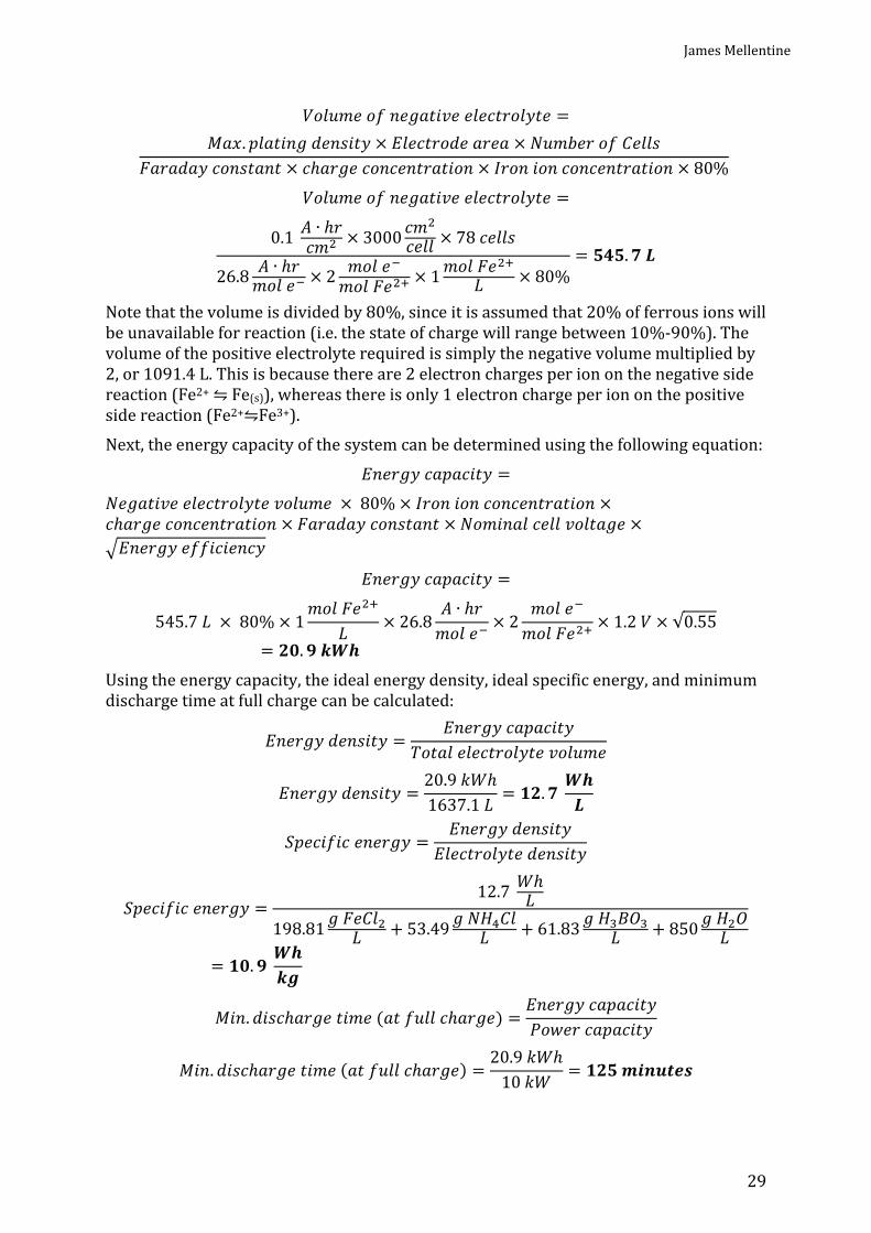
James Mellentine
29
= . × × × ℎ × × 80% = 0.1 ∙ ℎ × 3000 × 78 26.8 ∙ ℎ × 2 × 1 × 80% = . Note that the volume is divided by 80%, since it is assumed that 20% of ferrous ions will be unavailable for reaction (i.e. the state of charge will range between 10%-90%). The volume of the positive electrolyte required is simply the negative volume multiplied by 2, or 1091.4 L. This is because there are 2 electron charges per ion on the negative side reaction (Fe2+ ⇋ Fe(s)), whereas there is only 1 electron charge per ion on the positive side reaction (Fe2+⇋Fe3+). Next, the energy capacity of the system can be determined using the following equation: = × 80% × ×ℎ × × × = 545.7 × 80% × 1 × 26.8 ∙ ℎ × 2 × 1.2 × √0.55= . Using the energy capacity, the ideal energy density, ideal specific energy, and minimum discharge time at full charge can be calculated: =
= 20.9 ℎ1637.1 = . = = 12.7 ℎ198.81 + 53.49 + 61.83 + 850 = .
. ℎ ( ℎ ) = . ℎ ( ℎ ) = 20.9 ℎ10 =

Chapter 3: Cost Analysis of Iron Hybrid Flow Battery
30
The electrolyte pumps are assumed to pump at one and a half times the stoichiometric flow rate. The maximum flow rate will occur on the positive side when only 10% of ions remain unreacted. The following is the calculation for the required pump flow rate: . = × × × ℎ × × 10% . = 0.050 × 3000 × 78 26.8 ∙ ℎ × 1 × 1 × 10% × 1.5
= 6548 ℎ = . = Using this flow rate, the linear velocity of the electrolyte through the cell can be calculated. The flow rate is divided by the number of cells to get the flow rate per-cell, and then divided by the area normal to the direction of flow (product of cell width and thickness). = × ℎ × ℎ = 181978 × 60.96 × 0.318 = . Next, the felt compression is calculated. From the specifications sheet of Sigracell GFA5 graphite felt (produced by GSL Group), the graphite has a thickness of 5 mm (SGL Group, 2010). Against the assumed cell thickness of 3.18 mm, this represents a compression of 63.6%. This compression, along with the linear velocity of the electrolyte, was used to estimate the maximum pressure drop across the cell. Figure 3.1 shows data from a study related to a similar electrolyte flowing through a single cell with graphite felt (Gonzalez-Garcia, Montiel, Aldaz, Conesa, Perez, & Codina, 1998). In this study, the team used varying felt thicknesses inside of an 8 mm cell gap, and measured the pressure drop across the inlet and outlet of the cell. Figure 3.1 shows the linear electrolyte velocity in m/s along the x-axis and the pressure drop in Pascals (N/m2) along the y-axis. The various curves represent the different felt thicknesses, ranging from an empty cell to a felt thickness of 13 mm, which is equivalent to a compression of 61.5%, which is very close to the felt compression in the designed system in this study. At a maximum flow velocity of 1.2 cm/s, the measured pressure drop for the 13 mm felt was about 28,000 N/m2. However, this pressure drop must be adjusted upward to account for the fact that their cell height was only 12 cm. First, the pressure drop from only the felt was determined by subtracting the pressure drop from the empty cell at the same velocity. ∆ = ∆ + ∆ ∆ = 28,000 − 4800 2 = , The pressure increase was assumed to be linear with the height of the cell, so the pressure drop from the felt was multiplied by the ratio of heights.
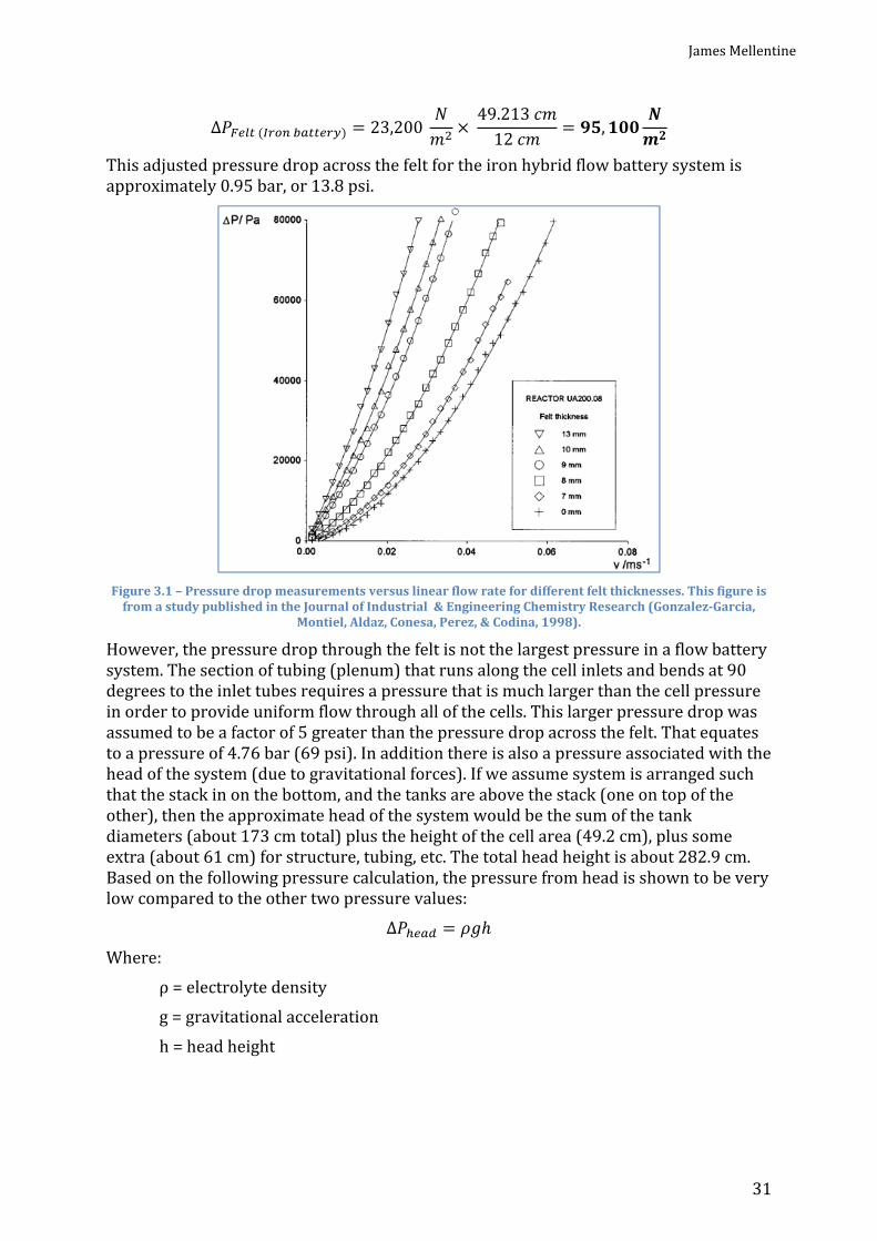
James Mellentine
31
∆ ( ) = 23,200 × 49.213 12 = , This adjusted pressure drop across the felt for the iron hybrid flow battery system is approximately 0.95 bar, or 13.8 psi.
Figure 3.1 – Pressure drop measurements versus linear flow rate for different felt thicknesses. This figure is
from a study published in the Journal of Industrial & Engineering Chemistry Research (Gonzalez-Garcia, Montiel, Aldaz, Conesa, Perez, & Codina, 1998). However, the pressure drop through the felt is not the largest pressure in a flow battery system. The section of tubing (plenum) that runs along the cell inlets and bends at 90 degrees to the inlet tubes requires a pressure that is much larger than the cell pressure in order to provide uniform flow through all of the cells. This larger pressure drop was assumed to be a factor of 5 greater than the pressure drop across the felt. That equates to a pressure of 4.76 bar (69 psi). In addition there is also a pressure associated with the head of the system (due to gravitational forces). If we assume system is arranged such that the stack in on the bottom, and the tanks are above the stack (one on top of the other), then the approximate head of the system would be the sum of the tank diameters (about 173 cm total) plus the height of the cell area (49.2 cm), plus some extra (about 61 cm) for structure, tubing, etc. The total head height is about 282.9 cm. Based on the following pressure calculation, the pressure from head is shown to be very low compared to the other two pressure values: ∆ = ℎ Where: ρ = electrolyte density g = gravitational acceleration h = head height

Chapter 3: Cost Analysis of Iron Hybrid Flow Battery
32
∆ = 198.81 + 53.49 + 61.83 + 851.5 9.81 (0.2829 ) = 32,391 = . = . The maximum total system pressure drop is estimated to be the sum of the three pressures: ∆ = ∆ + ∆ + ∆ = 0.95 + 4.76 + 0.3239 = . = . However, the pump flow rate is generally varied according to the stoichiometric reaction rate, or state of charge. The pump will not always run at the maximum rate. In chapter 4, the operations of the iron flow battery system is explored in an area regulation application. It was found that the average state of charge in that application is about 41.4%. Using the same equations as above, the average linear velocity of the electrolyte was calculated.
. = 0.050 × 3000 × 78 26.8 ∙ ℎ × 1 × 1 × 41.4% × 1.5= 1582 ℎ = . =
. = 43978 × 60.96 × 0.318 = . By using the same data in Figure 3.1, the pressure drop across the felt was estimated to be 5833 N/m2. Adjusting for same height ratio gives a ΔPfelt(avg) = 23,923 N/m2 = 0.239 bar = 3.47 psi. Multiplying this by five for the pressure drop across the inlet pipe results in a pressure drop across the inlet ΔPinlet(avg) = 119,600 N/m2 = 1.196 bar = 17.3 psi. Adding the pressure drop against the felt, the pressure drop across the inlet, and the same head pressure gives the average total pressure of the system. = 0.239 + 1.196 + 0.3239 = . = . As a check against the assumed parasitic losses, the pump power at this pressure level was calculated as a product of the total pressure and flow rate, divided by an assumed efficiency of 80%. = ( ) × ( )80% = 1.759 × 10 × (0.439 × 10 )80% = 96.5 Dividing the pump power by the total battery power of 10,000 W yields a parasitic loss of about 1.0% on the positive side pump. Since the pump on the negative side of the cell would run at half the speed and thus has approximately half the pressure drop (since there are two electrons per mole in the reaction instead of one on the positive side), an additional 25 W was added, bringing the total estimated parasitic loss to 1.25%, which

James Mellentine
33
is less than a quarter of the assumed 6% loss above. So that assumption is quite conservative. Table 3.2 shows consolidated results of calculated performance characteristics of the designed system: Table 3.2 – Calculated system and performance characteristics for a 10 kW/20.9 kWh iron flow battery system.
System/Performance Characteristic
Value System/Performance Characteristic
Value
Power density 48 mW/cm2 Energy capacity 20.9 kWh Power per-cell 145.1 W Energy density 12.7 Wh/L Number of cells 78 Specific energy 10.9 Wh/kg Stack voltage 75.5 V Minimum discharge time at full charge 125 minutes Electrolyte volume (Negative/Positive/Total) 545.7 L/1091.4 L/1637.1 L Shunt loss 10 W
Pump flow rate 109.1 L/min Average internal pressure 1.76 bar 3.2 Component Cost Estimation Methodology and Results With the size and performance characteristics of the stack calculated, the next step in the design process is to calculate how much of each component is needed for an annual production estimate of 1000 units, and then obtain price estimates for each component. The activated graphite felt will go on both sides of the cell, and thus two times the active area will be needed for each system. . = 0.6 × 78 × 1000 = , A manufacturer could purchase that amount of felt for an estimated price of $90/m2 for 0.635 cm thick felt. An optimistic price is $80/m2 and a pessimistic price is $100/m2 (Tanzola, 2010). A system with 78 cells will need 77 bipolar plates and 2 end-of-stack electrodes. For simplicity, this study assumes 79 bipolar plates for each stack since the composition and size is so similar to the end-of-stack electrodes. = 79 × 1000 = , A manufacturer could purchase that number of 0.3 m2 bipolar plates for an estimated price of $50/plate. This assumes a standard molded manufacture. An optimistic price is $35/plate and a pessimistic price is $55/plate (Tanzola, 2010). Regarding flow frames, the assumed design is one in which a single flow frame contains flow channels for both of the adjacent cells. The flow frame is a 2-piece assembly, but considered 1 part. A system with 78 cells will need 79 flow frames.

Chapter 3: Cost Analysis of Iron Hybrid Flow Battery
34
= 79 × 1000 = , A manufacturer could purchase that number of flow frames for an estimated price of $32/frame. This assumes an injection-molded polymer material in a 2-part assembly. An optimistic price is $25/frame and a pessimistic price is $60/frame (Tanzola, 2010). Each cell requires a gasket to seal the system. For this system, a Viton rubber o-ring gasket could be molded to match the contour of the frame. A system with 78 cells will need 154 gaskets (2 for each of the 76 internal cells and 1 each for the 2 end cells). = 154 × 1000 = , A manufacturer could purchase that number of gaskets for an estimated price of $2/gasket. An optimistic price is $1/gasket and a pessimistic price is $2.50/gasket (Tanzola, 2010). Two gold-plated copper collectors are needed for each unit. = 2 × 1000 = , The price of this product depends highly on the current market price of copper. Currently, a manufacturer could purchase that number of collector plates for an estimated price of $125/plate, with a pessimistic price of $150/plate (Tanzola, 2010). An optimistic price was calculated by taking the 2010 average market price of copper ($3.42/lb) and gold ($1224.53/troy ounce) and adding a 25% manufacturing cost (BNA, 2010) (Austin Gold Information Network, 2011). If we assume a copper thickness of 1/16 inch (0.15875 cm), and the area is the active area plus a 1 cm band around the outside (3224.4 cm2 total), we know that each plate contains 4.58 kg of copper. At the 2010 average market price of $3.42/lb, that is $34.46 per plate. If we assume that one side of the plate is electroplated with a standard 0.175 microns of gold, each plate will have 1.09 g, which has a cost of $42.91 at the market price noted above. Taking the sum of the copper and gold and adding 25% for manufacturing yields a total plate cost of $96.63. This is considered the optimistic cost for this part. Similarly, two aluminum end plates are needed for each unit. = 2 × 1000 = , The price of this product depends highly on the current market price of aluminum. Currently, a manufacturer could purchase that number of end plates for an estimated price of $175/plate, with a pessimistic price of $192.50/plate (Tanzola, 2010). Similar to the copper collector plate, an optimistic price was calculated by taking the 2010 average market price of aluminum ($2173.01/tonne) and adding a 25% manufacturing cost (Index Mundi, 2011). Assuming an aluminum thickness of 3 cm, and the area is extended 3 cm beyond the flow frames on each side (3921.4 cm2 total), then each plate contains 31.76 kg of aluminum. At the 2010 average market price of $2173.01/tonne, that is $69.02 per plate. Adding 25% for manufacturing yields a total plate cost of $86.28. This is considered the optimistic cost for this part.

James Mellentine
35
In this system, long stainless steel bolts will go through the aluminum end plates to compress the cells together. Three bolts will be on each edge, with a total of twelve bolts per unit. = 3 × 4 × 1000 = , A manufacturer could purchase that number of bolts for an estimated price of $12.50/bolt. An optimistic price is $10/bolt and a pessimistic price is $15/bolt (Tanzola, 2010). Each unit will require a series of polyvinyl chloride (PVC) plumbing parts and connections, including pipes, valves, joints, and end plates. This study will consider all of these pieces as 1 “set” per unit. = 1 × 1000 = , An estimated wholesale price of $150/set was provided by InnoVentures. An optimistic price is $100/set and a pessimistic price is $200/set (Tanzola, 2010). Each cell requires a membrane separator. The separator area is slightly larger than the active area. Assuming a 1 cm border around the active area, this adds 218.4 cm2 to each cell. This cost model assumes a microporous separator that was also used during parallel experiments – the DP-34-14 by Daramic (polyethylene microporous material). . = (0.3 + .02184) × 78 × 1000 = , To produce custom-size sheet lengths to accommodate this system, a representative from Daramic provided an estimated price of $4.35/m2, with an optimistic price of $3.50/m2 and a pessimistic price of $5/m2 (Roe, 2010). However, in laboratory testing (detailed in a later chapter), a significant amount of electrolyte crossover was observed when using microporous membranes. A non-porous ion exchange membrane was able to prevent this behavior. In order to solve this problem in a commercial system, it may be necessary to reduce the porosity of the microporous membrane, or enhance it in some other way that drastically increases its cost. The thesis supervisor suggested a pessimistic price of $80/m2 to account for this potential modification. Next, the electrolyte components were estimated. The electrolyte composition is the same on both the negative and positive side of the battery, and the total electrolyte volume per unit is approximately 1638 L. For the ferrous chloride, ammonium chloride, and boric acid, the annual amounts were calculated as follows: = ℎ × ℎ × 1638 × 1000
= 1 × 126.75 × 1638 × 1000 = , = 1 × 53.49 × 1638 × 1000 = ,
= 1 × 61.83 × 1638 × 1000 = ,

Chapter 3: Cost Analysis of Iron Hybrid Flow Battery
36
After contacting several chemical companies, a representative from Brenntag Group was able to provide estimates for the ammonium chloride and the boric acid. For ammonium chloride, the estimated cost is $1.06/kg, with an optimistic price of $0.86/kg and a pessimistic price of $1.12/kg. For boric acid, the estimated price is $1.96/kg, with an optimistic price of $1.63/kg and a pessimistic price of $2.09/kg (Battaglia, 2011). A representative from PVS Chemicals was able to provide price estimates for large quantities of 27% ferrous chloride solution. The specific gravity of the solution is 1.325. The amount of solution equivalent to the annual mass requirement was calculated: ( % )= 207,617 27 100 × (1.325 × 998.2) × 1000= ,
This is equivalent to 153,603 gallons per year. Since the solution is delivered via 4000-gallon tanker truck, about 38 full deliveries per year would be required. At this volume, PVS chemicals estimated a price between $0.30 to $0.68 per gallon, with an average of $0.49 per gallon (Bennett, 2011). Regarding the de-ionized water in which the other chemicals are dissolved, parallel experiments showed that about 850 mL of water were needed per liter of electrolyte solution. However, in a commercial system the ferrous chloride solution would be further diluted with water while the other chemicals are added. The volume of additional water was calculated to be 92% of the total volume of solution minus the volume of the ferrous chloride solution: = 1638 × 92% × 1000 − 581,386 = , Price information for de-ionized water is also difficult to find. The primary options are to have it delivered in large tanks or to produce it on-site using water purification systems. Mike Konrad, CEO of Aqueous Technologies, estimates that the average cost of de-ionized water is about 6 cents per gallon, or about 1.6 cents per liter (Konrad, 2009). In the absence of an optimistic quote, this price was also used. As a pessimistic quote, I used the price for delivered water from Brenntag, 23.8 cents per liter (Battaglia, 2011). Adding the most likely prices of all the chemicals together and dividing by the volume of electrolyte to be produced, the most likely cost of electrolyte was determined to be 23.3 cents per liter, or 88.1 cents per gallon. = (581,386 × $0.129/ ) + (87,617 × $1.06/ ) + (101,278 × $1.96/ ) + (925,574 × $0.016/ )1,638,000 = $ . = $ . /⁄ A small amount of labor will be needed to produce the electrolyte, but it is a much simpler process compared to vanadium redox systems. The chemicals can literally be measured and poured into the water and mixed for a short period until it is dissolved completely. The author has completed this task in the lab many times, and it would not be very different in a commercial setting. The author estimates that large batches of

James Mellentine
37
electrolyte could be mixed twice per week and divided among the manufactured units, with a single batch fulfilling the needs of 10 units. ℎ = 1000 10 ℎ =
Assuming a labor cost of $50/person-hour and preparation time of 2 hours per batch, the cost for electrolyte preparation per-batch was estimated at $100, with an optimistic cost of $50 (1 hour) and a pessimistic price of $150 (3 hours). Each unit will have 1 large tank for the positive electrolyte and 1 smaller tank for the negative electrolyte, or 1000 tanks of each size per year. A distributor for Den Hartog Industries provided an estimate of $109.76 for a 150-gallon (568-liter) medium density polyethylene (MDPE) tank, with the same price as the optimistic estimate and $126.04 as the pessimistic estimate. An estimate of $167.21 was provided for a 300-gallon (1136-liter) MDPE tank, with the same price as the optimistic estimate and $192.01 as the pessimistic estimate (Samuelson, 2011). Next, two pumps per unit will be required to pump the electrolyte through the cell. To resist corrosion from the electrolyte and to avoid taking part in the reaction, the parts exposed to the electrolyte would need to be non-metallic. InnoVentures recommends using a small centrifugal pump with polymer/ceramic inner lining. A price estimate for such a pump that can handle the flow rate and pressure calculated above is about $200. An optimistic price is $100, with a pessimistic price of $300 (Tanzola, 2010). Finally, a control system is needed to regulate the operations of the battery. Prices for this can vary widely depending on whether the circuit board is custom made or off-the-shelf. An estimate of $600/unit was used, with an optimistic price of $100 if a small simple circuit board were custom made. A pessimistic price is $800 (Tanzola, 2010). Table 3.3 summarizes the quantities and prices for each of the components mentioned in this section.
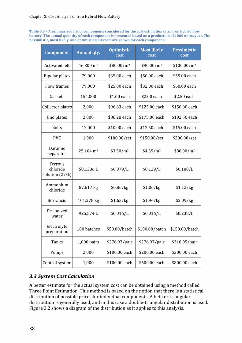
Chapter 3: Cost Analysis of Iron Hybrid Flow Battery
38
Table 3.3 – A summarized list of components considered for the cost estimation of an iron hybrid flow battery. The annual quantity of each component is presented based on a production of 1000 units/year. The pessimistic, most likely, and optimistic unit costs are shown for each component.
Component Annual qty. Optimistic cost
Most likely cost
Pessimistic cost Activated felt 46,800 m2 $80.00/m2 $90.00/m2 $100.00/m2 Bipolar plates 79,000 $35.00 each $50.00 each $55.00 each Flow frames 79,000 $25.00 each $32.00 each $60.00 each Gaskets 154,000 $1.00 each $2.00 each $2.50 each Collector plates 2,000 $96.63 each $125.00 each $150.00 each End plates 2,000 $86.28 each $175.00 each $192.50 each Bolts 12,000 $10.00 each $12.50 each $15.00 each PVC 1,000 $100.00/set $150.00/set $200.00/set Daramic separator 25,104 m2 $3.50/m2 $4.35/m2 $80.00/m2
Ferrous chloride solution (27%) 581,386 L $0.079/L $0.129/L $0.180/L Ammonium chloride 87,617 kg $0.86/kg $1.06/kg $1.12/kg Boric acid 101,278 kg $1.63/kg $1.96/kg $2.09/kg De-ionized water 925,574 L $0.016/L $0.016/L $0.238/L Electrolyte preparation 100 batches $50.00/batch $100.00/batch $150.00/batch
Tanks 1,000 pairs $276.97/pair $276.97/pair $318.05/pair Pumps 2,000 $100.00 each $200.00 each $300.00 each Control system 1,000 $100.00 each $600.00 each $800.00 each 3.3 System Cost Calculation A better estimate for the actual system cost can be obtained using a method called Three Point Estimation. This method is based on the notion that there is a statistical distribution of possible prices for individual components. A beta or triangular distribution is generally used, and in this case a double-triangular distribution is used. Figure 3.2 shows a diagram of the distribution as it applies to this analysis.

James Mellentine
39
Figure 3.2 – An example distribution of component prices. The x-axis is the estimated component price, and the y-axis is the probability of each price being the real price. Price “a” is an optimistic (low) price, Price “m”
is the most likely price (highest probability), and Price “b” is a pessimistic (high) price. For each component a weighted average, or “expected” cost, and a standard deviation can be calculated using the following formulas governing double-triangular distribution (Lehmann, 2008). = ( + 4 + )6 = ( − )6 First, the expected cost and standard deviation of the activated felt was calculated per battery system. From the price estimates in the previous section, = 46.8 × $80 = $3,744
= 46.8 × $90 = $4,212 = 46.8 × $100 = $4,680
= (3744 + 4(4212) + 4680)6 = $ , = (4500 − 3600)6 = $ Next, a variance value is calculated for each component, which is equal to the square of the standard deviation. So, for the activated felt component: = (150) = , These calculations were repeated for each component. The expected cost, standard deviation, and variance for each component are shown in Table 3.4, along with the sum of the expected cost and variance values.

Chapter 3: Cost Analysis of Iron Hybrid Flow Battery
40
Table 3.4 – For each component of the iron hybrid flow battery system, the calculated values of expected cost, standard deviation, and variance are shown. These values are based on the Three Point Estimation method.
Component Expected Cost Standard Deviation Variance Activated felt $4,212.00 $156.00 24,336.00 Bipolar plates $3,818.33 $263.33 69,344.44 Flow frames $2,804.50 $460.83 212,367.36 Gaskets $295.17 $38.50 1,482.25 Collector plates $248.88 $17.79 316.47 End plates $326.26 $35.41 1,253.70 Bolts $150.00 $10.00 100.00 PVC $150.00 $16.67 277.78 Daramic separator $422.93 $320.66 102,823.56 Ferrous chloride solution, 27% $75.27 $9.73 94.64
Ammonium chloride $90.72 $3.78 14.31 Boric acid $195.40 $7.82 61.09 De-ionized water $73.57 $51.50 2,652.10 Electrolyte preparation $10.00 $1.67 2.78 Tanks $283.82 $6.85 46.88 Pumps $400.00 $66.67 4,444.44 Control system $550.00 $116.67 13,611.11 Total $14,082.18 - 431,748.87 From this data, we see that the total expected cost of the 10 kW, 20.9 kWh system is $14,082. The breakdown of system costs are shown in Figure 3.3. Unlike the vanadium redox battery cost breakdown shown in Chapter 1, the electrolyte and preparation are only a very small percent (~ 3%) of the total expected system cost. The largest costs for the system are the activated felt, bipolar plates, and flow frames – 30%, 27%, and 20%, respectively.

James Mellentine
41
Figure 3.3 – Individual component costs as a percent of total system cost for a 10 kW, 20.9 kWh iron hybrid
flow battery system. The largest costs of the system are the activated felt, bipolar plates, and flow frames. The cost of electrolyte and preparation is about 3% of the total cost. The next goal of the three point estimation method is to determine the maximum cost of the system with a specific confidence level. The first step to achieve this is to calculate the standard deviation of the total variance by taking the square root of the total variance value (calculated in the table above). . . = 431,748.87 = $ . Next, a decision was made on what the confidence level would be. For this project, it is desirable to have a reasonably high level of confidence in the cost of the system. However, it is not necessary to have absolute certainty. The author chose a confidence level of 90%. In a normal statistical distribution, 90% represents about 1.282 standard deviations (also known as a Z-value). To estimate the maximum cost of the system with a 90% confidence level, the Z-value is multiplied by the standard deviation of the variance, and the resulting product is added to the total expected cost. % = $14,082.18 + ($657.08 × 1.282) = $ , . This result means that the battery system can be built for $14,924 or less with 90% confidence. Dividing that cost by the power rating of 10 kW gives the cost per kW, or $1492/kW. Dividing the total cost by the energy rating of 20.9 kWh gives the cost per kWh, or $715/kWh.
3.4 Sensitivity Analysis For the manufacturer of such a battery system, it may be interesting to know what the major cost drivers are. Which component prices have the largest effect on the cost per kW and cost per kWh? Which performance factors have the largest effect on the cost per kW and cost per kWh? This information can help to focus research and development or component acquisition strategies to drive down the cost of the system.

Chapter 3: Cost Analysis of Iron Hybrid Flow Battery
42
To calculate this information, the data table functionality in Microsoft Excel was used. Refer to Appendix A for the complete cost model spreadsheet that includes these data table calculations. For each component, the unit price was varied from -50% to 50% of the expected cost (Table 3.4) and the resulting cost per kW and per kWh with 90% confidence was re-calculated to determine the effect of varying the unit price. The result of this analysis on cost per kW is shown in Figure 3.4. The graph shows the percent variation in expected component price on the x-axis, and the resulting system cost per kW (with 90% confidence) on the y-axis. A clear conclusion from this graph is that the unit prices of the activated felt, the bipolar plates, and the flow frames have the greatest effect on the total system cost (+/- $160/kW-$220/kW). The other component prices have only a slight effect (less than +/- $30/kW) on the total price. This is not necessarily a surprising result since the same three components make up the largest share of the total system cost. To drive down the price of this system, efforts should be focused on lowering cost of the felt, bipolar plates, and flow frame.
Figure 3.4 – The sensitivity of the system cost per kW based on the variation of each expected component price is shown. The unit price of the activated felt, bipolar plates, and flow frames are shown to have the
greatest impact on cost per kW. Other unit prices have only a slight effect. The result of this analysis on cost per kWh is shown in Figure 3.4. The graph shows the percent variation in expected component price on the x-axis, and the resulting system cost per kWh (with 90% confidence) on the y-axis. The same conclusion can be drawn from this graph - the unit prices of the activated felt, the bipolar plates, and the flow frames have the greatest effect on the system cost per kWh (+/- $80/kWh-$105/kWh). The other component prices have only a slight effect (less than +/- $15/kWh) on the total price. This is not necessarily a surprising result since the same three components

James Mellentine
43
make up the largest share of the total system cost. To drive down the price of this system, efforts should be focused on lowering cost of the felt, bipolar plates, and flow frame.
Figure 3.5 - The sensitivity of the system cost per kWh based on the variation of each expected component
price is shown. The unit price of the activated felt, bipolar plates, and flow frames are shown to have the greatest impact on cost per kWh. Other unit prices have only a slight effect. For evaluating performance characteristic values against total system price, five values were chosen that have the potential to be improved through research and development: current density, iron concentration, plating density, voltaic efficiency, and coulombic efficiency. For each of these performance characteristics, the performance was varied from -50% to 50% of the assumed value (Table 3.1) and the resulting system cost per kW and per kWh with 90% confidence was re-calculated to determine the effect of varying the performance. The result of this analysis per kW is shown in Figure 3.6. Note that coulombic efficiency is not included on this graph since it only effects energy capacity and not power capacity, therefore it has no effect on cost per kW. The graph shows the percent variation in performance on the x-axis, and the resulting system cost per kW (with 90% confidence) on the y-axis. A clear conclusion from this graph is that the variation in current density and voltaic efficiency has the greatest effect on the cost per kW. An increase in the current density of 20% (to 60 mA/cm2) would lower the total system cost by over $200/kW. An increase of 40% in voltaic efficiency (to 91%) would achieve a similar result. However, this is approaching (or exceeds) the practical limit of the voltaic efficiency since some overvoltage is necessary to operate the battery. Increasing the iron concentration in the electrolyte by 50% (to 1.5 M) would decrease the cost of the battery by only about $12/kW. This makes sense considering the cost of the electrolyte is such a low percent of the cost of the entire system, so decreasing the

Chapter 3: Cost Analysis of Iron Hybrid Flow Battery
44
volume would not have much effect. An increase in plating density would slightly increase the cost of the battery on a per kW basis. The plating density affects energy capacity only and does not affect power capacity. Increasing the plating capacity serves only to increase the energy capacity, and thus increase the required electrolyte volume and the overall cost per kW. However, plating capacity does decrease cost on a per kWh basis as shown later. To drive down the price of this system on a per kW basis, efforts should be focused on increasing the maximum operating current density, with a secondary focus on increasing the voltaic efficiency (to the extent possible).
Figure 3.6 – The sensitivity of the system cost per kW based on the variation of four performance factors is
shown. The improvement of the current density and voltaic efficiency are shown to have the greatest impact on cost per kW. An increasing iron concentration would have only a slight impact on cost, while an increase
in plating density would actually increase the cost per kW slightly due to increased electrolyte volume. The result of this analysis per kWh is shown in Figure 3.7. The graph shows the percent variation in performance on the x-axis, and the resulting system cost per kWh (with 90% confidence) on the y-axis. A clear conclusion from this graph is that the variation in plating density, voltaic efficiency, and coulombic efficiency has the greatest effect on the cost per kWh. An increase in the plating density of 50% (to 150 mA-hr/cm2) would lower the system cost by over $225/kWh. An increase of 17% in coulombic efficiency (to 99.5%) would lower the system cost by about $60/kWh. Increasing the voltaic efficiency by 20% (to 78%) would have a similar effect. Increasing the iron concentration in the electrolyte by 50% (to 1.5 M) would decrease the cost of the battery by only about $5/kWh. An increase in current density would slightly increase the cost of the battery on a per kWh basis. The increased current density would decrease the required active area and in effect reduce the overall electrode area that is available for plating. This would in turn decrease the energy capacity of the battery, and
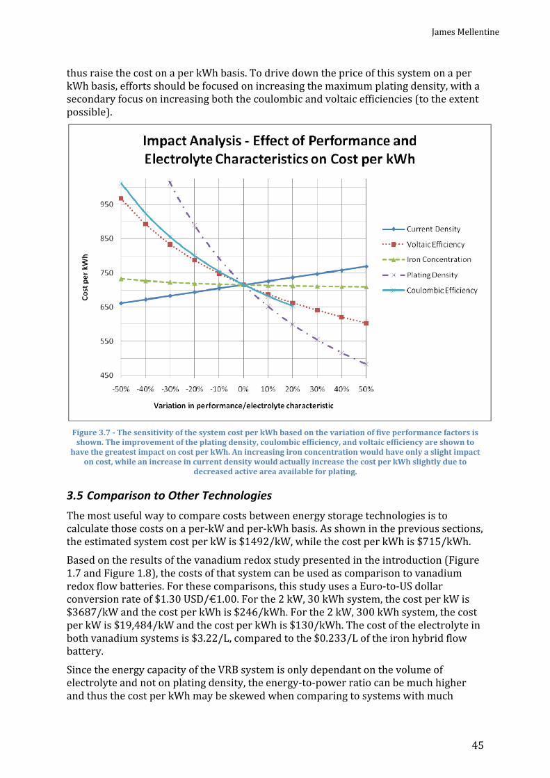
James Mellentine
45
thus raise the cost on a per kWh basis. To drive down the price of this system on a per kWh basis, efforts should be focused on increasing the maximum plating density, with a secondary focus on increasing both the coulombic and voltaic efficiencies (to the extent possible).
Figure 3.7 - The sensitivity of the system cost per kWh based on the variation of five performance factors is
shown. The improvement of the plating density, coulombic efficiency, and voltaic efficiency are shown to have the greatest impact on cost per kWh. An increasing iron concentration would have only a slight impact
on cost, while an increase in current density would actually increase the cost per kWh slightly due to decreased active area available for plating.
3.5 Comparison to Other Technologies The most useful way to compare costs between energy storage technologies is to calculate those costs on a per-kW and per-kWh basis. As shown in the previous sections, the estimated system cost per kW is $1492/kW, while the cost per kWh is $715/kWh. Based on the results of the vanadium redox study presented in the introduction (Figure 1.7 and Figure 1.8), the costs of that system can be used as comparison to vanadium redox flow batteries. For these comparisons, this study uses a Euro-to-US dollar conversion rate of $1.30 USD/€1.00. For the 2 kW, 30 kWh system, the cost per kW is $3687/kW and the cost per kWh is $246/kWh. For the 2 kW, 300 kWh system, the cost per kW is $19,484/kW and the cost per kWh is $130/kWh. The cost of the electrolyte in both vanadium systems is $3.22/L, compared to the $0.233/L of the iron hybrid flow battery. Since the energy capacity of the VRB system is only dependant on the volume of electrolyte and not on plating density, the energy-to-power ratio can be much higher and thus the cost per kWh may be skewed when comparing to systems with much

Chapter 3: Cost Analysis of Iron Hybrid Flow Battery
46
higher energy capacity. So in addition to comparing to the systems in the study, an “adjusted” vanadium system cost was calculated based on scaling down the volume of electrolyte such that the energy capacity was 4 kWh, roughly the same energy-to-power ratio as the iron hybrid flow battery designed in this study. To scale down the 30 kWh system to 4 kWh, the amount of vanadium pentoxide was also scaled down by the same ratio. = €2448 × 430 = € . = €5673 − €2448 + €326.4 = € . In this adjusted case with the same energy-to-power ratio, the vanadium system cost is $2308/kW and $1154/kWh. Comparisons to zinc-bromine flow batteries can be made based on published cost estimates on the website of ZBB Energy, one of the largest manufacturers of zinc bromine systems. According to a presentation on their website, they can manufacture their current systems at a cost of $800/kWh (ZBB Energy). Since the energy-to-power ratio of their main product is 2:1, that equates to a price of $1600/kW. The energy- and power-specific prices of the iron hybrid flow battery are compared to the vanadium redox, zinc bromine, and other technologies in Figure 3.8. On a per-kW basis, the proposed iron hybrid flow battery costs less than all of the other flow battery systems, but still much higher than the lowest costs of other energy storage technologies as previously depicted in Figure 1.3. On a per-kWh basis, the proposed iron hybrid flow battery has a lower cost than the commercial zinc bromine system and the “adjusted” vanadium flow battery system. However, the vanadium redox systems with a higher energy capacity have a much lower cost per kWh. This is due to the inherent limitations on the energy-to-power ratio of the iron hybrid flow battery. The per-kWh cost is much less than electrochemical capacitors and flywheels, but much higher than long-duration electrochemical capacitors, pumped hydro, and CAES.

James Mellentine
47
Figure 3.8 – the per kW and per kWh costs for the iron hybrid flow battery are compared to the vanadium
redox flow battery, zinc bromine hybrid flow battery, and other energy storage systems.

Chapter 3: Cost Analysis of Iron Hybrid Flow Battery
48

James Mellentine
49
Chapter 4: Performance in an Area Regulation Application This chapter proposes an application for the iron hybrid flow battery system designed in Chapter 3, and analyzes its performance in the application. The following sections discuss the methodology for selecting an appropriate application, operating assumptions, and performance results. 4.1 Methodology and Application Selection An introduction to possible large-scale grid storage applications was presented above in section 1.1.3. Most of those applications can be eliminated for an iron hybrid flow battery based on discharge time alone. As determine in Chapter 3, the maximum discharge time for this battery is about 2 hours. Most of the applications listed in Table 1.2 require a minimum discharge time of 2 hours or more. Eliminating these applications results in the list presented in Table 4.1. The transmission support application was also eliminated due to the extremely short discharge time requirement. The response time of this system has not been studied and it is not clear if it could be ready to operate within the second-or-less timescale that would be required. Table 4.1 – After removing several applications from Table 1.2 based on discharge time requirements, this is a list of possible applications for an iron hybrid flow battery, Data sourced from a Sandia National Laboratories report (Eyer & Corey, 2010).
Application Power Discharge Time # Description Low High Low High 4 Area Regulation 1 MW 40 MW 15 min. 30 min.5 Electric Supply Reserve Capacity 1 MW 500 MW 1 hr. 2 hr. 6 Voltage Support 1 MW 10 MW 15 min. 1 hr. 13 Electric Service Reliability 0.2 kW 10 MW 5 min. 1 hr. 14 Electric Service Power Quality 0.2 kW 10 MW 10 sec. 1 min. 17.1 Wind Generation Grid Integration, Short Duration 0.2 kW 500 MW 10 sec. 15 min.17.2 Wind Generation Grid Integration, Long Duration 0.2 kW 500 MW 1 hr. 6 hr. Of the remaining applications, the one with the highest benefit ($/kW) is area regulation. In the Sandia study, the estimated benefit for area regulation was calculated to be $785/kW - $2010/kW, based on a 10-year system lifetime, 2.5% price escalation rate, and 10% discount rate (Eyer & Corey, 2010). Therefore, area regulation was selected as a basis for analyzing the performance of the proposed iron hybrid flow battery system1. (See footnote at end of chapter). Note that the estimated market for area regulation is significantly lower than the market for other applications, with an estimated United States market potential of 1012 MW over the next 10 years – or about 101 MW of capacity per year. In terms of the annual production volumes estimated in Chapter 3, this is still a large market. The proposed production of 1000 units with 10 kW capacity is equal to 10 MW per year. This is only 10% of the smallest market grid storage application market, leaving considerable room for growth and competition. The typical storage capacity for a single facility is between 1 MW and 40 MW, so a 10 kW unit is obviously too small. So for this application, it is proposed that a number of these units will be connected in series as modules that compose a larger unit. A

Chapter 4: Performance in an Area Regulation Application
50
somewhat arbitrary size of 2 MW was selected for this study, which would be composed of 200 modular 10 kW units. This same modular approach is used by other flow battery companies such as ZBB Energy. For this analysis, area regulation data was obtained from the California Independent Service Operator (CAISO). They publish the amount of area regulation capacity purchased per hour, along with the price paid for the service. This data was aggregated for the year of 2008 (the latest full year available). Next, a set of operating assumptions was made based on the case study presented in the Sandia study (discussed in the next section). The battery state of charge was then calculated for each hour of the year based on the charge and discharge usage. The total number of cycles per year was calculated, along with the average state of charge, the total area regulation revenue, and the energy costs and sales associated with charge and discharge operations. 4.2 Project Assumptions Area regulation is an ancillary grid service that matches grid capacity with consumer demand in real time. To maintain grid voltage and frequency values within preset limits, the power capacity of the grid must be closely matched to the actual grid demand at any given time. For example, if 100 people in a city simultaneously turn on or shut off a 100 W light bulb, the capacity demand would instantly go up or down by 10 kW. In addition to normal grid energy capacity, the regional grid operator must pay for area regulation services that can respond to this real-time demand change by ramping up and down. “Up Regulation” is the term used to describe the regulation service that adds capacity to the grid. “Down Regulation” is the term used to describe the regulation service that removes capacity from the grid. Figure 4.1 shows how area regulation service helps regulate the real-time grid capacity (Eyer & Corey, 2010).
Figure 4.1 – Visual example of how area regulation services are applied to the load curve. This diagram comes
from a study by Sandia National Laboratory (Eyer & Corey, 2010). Traditionally, area regulation has been provided by automatically-controlled power plants that have the ability to quickly ramp up and down, such as gas turbines. Energy storage can also fulfill this application by absorbing energy for down regulation or discharging for up regulation. If the battery is fully charged, it can only be available for up regulation. Likewise, if the battery is fully discharged, it can only be available for down regulation.

James Mellentine
51
A grid operator pays on a MW-per-hour basis for available capacity when it comes to area regulation, even if the capacity is never used. The amount paid for an hour of availability usually depends on a market-based bidding approach, where plant operators submit bids each hour (in an hour-ahead market) to provide the service. This is the approach used in California. This can be different in other markets, depending on how the electrical grid is regulated in a particular market. Also, a regulation facility is not always used during the time in which it is paid to be available. A regulation plant or battery can receive revenue for an hour of available capacity even if no service is provided during that hour. It should also be noted that a battery providing these services must purchase and sell the energy it used at the market rate. For example, the energy absorbed during down regulation must be purchased. The energy discharged during up regulation is sold at the same rate (assuming no time-of-use pricing structure). Since no storage technology is 100% efficient, more energy is always purchased than is sold, representing a net cost to the battery operator. A lower efficiency represents a larger cost. The cost also increases with the amount of regulation provided. According to the Sandia report, the discharge time required for providing area regulation service ranges from 15 to 30 minutes (Eyer & Corey, 2010). This analysis assumes that the battery provides up regulation or down regulation for 30 minutes during each hour that it is available, and that the battery operator receives the market price revenue for each hour that it is available. Since it is not known whether charge or discharge services will be needed, this was determined by a binary random number generator (0 = up regulation, 1 = down regulation). If the battery state of charge was above the threshold where it could not provide 30 minutes of down regulation, it was only made available for up regulation and only received the revenue for that service during that hour. Likewise, if the battery state of charge was below the threshold where it could not provide 30 minutes of up regulation, it was only made available for down regulation and only received the revenue for that service during that hour. The battery operating condition assumptions were consistent with the cost model assumptions. The state of charge was limited to operating between 10% and 90%. The round-trip energy efficiency of the battery was assumed to be 55%, while the parasitic and inverter losses were assumed to be 12%. The market price of up and down area regulation services were obtained from the California ISO website for each hour in 2008 (CAISO, 2009). This data was consolidated into a spreadsheet for this analysis. When the total revenues were calculated, they were multiplied by 3 years of 2.5% price escalation, consistent with the escalation rate used in the Sandia report. The energy purchase and sales rate used was $163.3/MWh, which was the commercial electricity rate in California as of September 2010 (EIA, 2011). Table 4.2 shows a summary of the assumptions for the analysis of an iron hybrid flow battery system in an area regulation application.
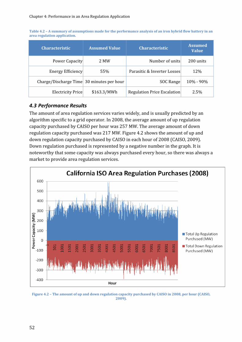
Chapter 4: Performance in an Area Regulation Application
52
Table 4.2 – A summary of assumptions made for the performance analysis of an iron hybrid flow battery in an area regulation application.
Characteristic Assumed Value Characteristic Assumed Value Power Capacity 2 MW Number of units 200 units Energy Efficiency 55% Parasitic & Inverter Losses 12% Charge/Discharge Time 30 minutes per hour SOC Range 10% - 90% Electricity Price $163.3/MWh Regulation Price Escalation 2.5%
4.3 Performance Results The amount of area regulation services varies widely, and is usually predicted by an algorithm specific to a grid operator. In 2008, the average amount of up regulation capacity purchased by CAISO per hour was 257 MW. The average amount of down regulation capacity purchased was 217 MW. Figure 4.2 shows the amount of up and down regulation capacity purchased by CAISO in each hour of 2008 (CAISO, 2009). Down regulation purchased is represented by a negative number in the graph. It is noteworthy that some capacity was always purchased every hour, so there was always a market to provide area regulation services.
Figure 4.2 – The amount of up and down regulation capacity purchased by CAISO in 2008, per hour (CAISO,
2009).
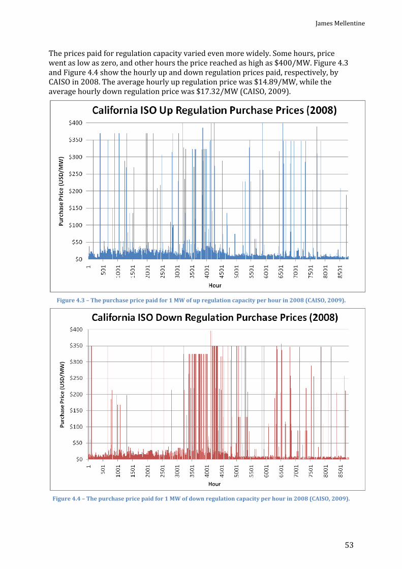
James Mellentine
53
The prices paid for regulation capacity varied even more widely. Some hours, price went as low as zero, and other hours the price reached as high as $400/MW. Figure 4.3 and Figure 4.4 show the hourly up and down regulation prices paid, respectively, by CAISO in 2008. The average hourly up regulation price was $14.89/MW, while the average hourly down regulation price was $17.32/MW (CAISO, 2009).
Figure 4.3 – The purchase price paid for 1 MW of up regulation capacity per hour in 2008 (CAISO, 2009).
Figure 4.4 – The purchase price paid for 1 MW of down regulation capacity per hour in 2008 (CAISO, 2009).
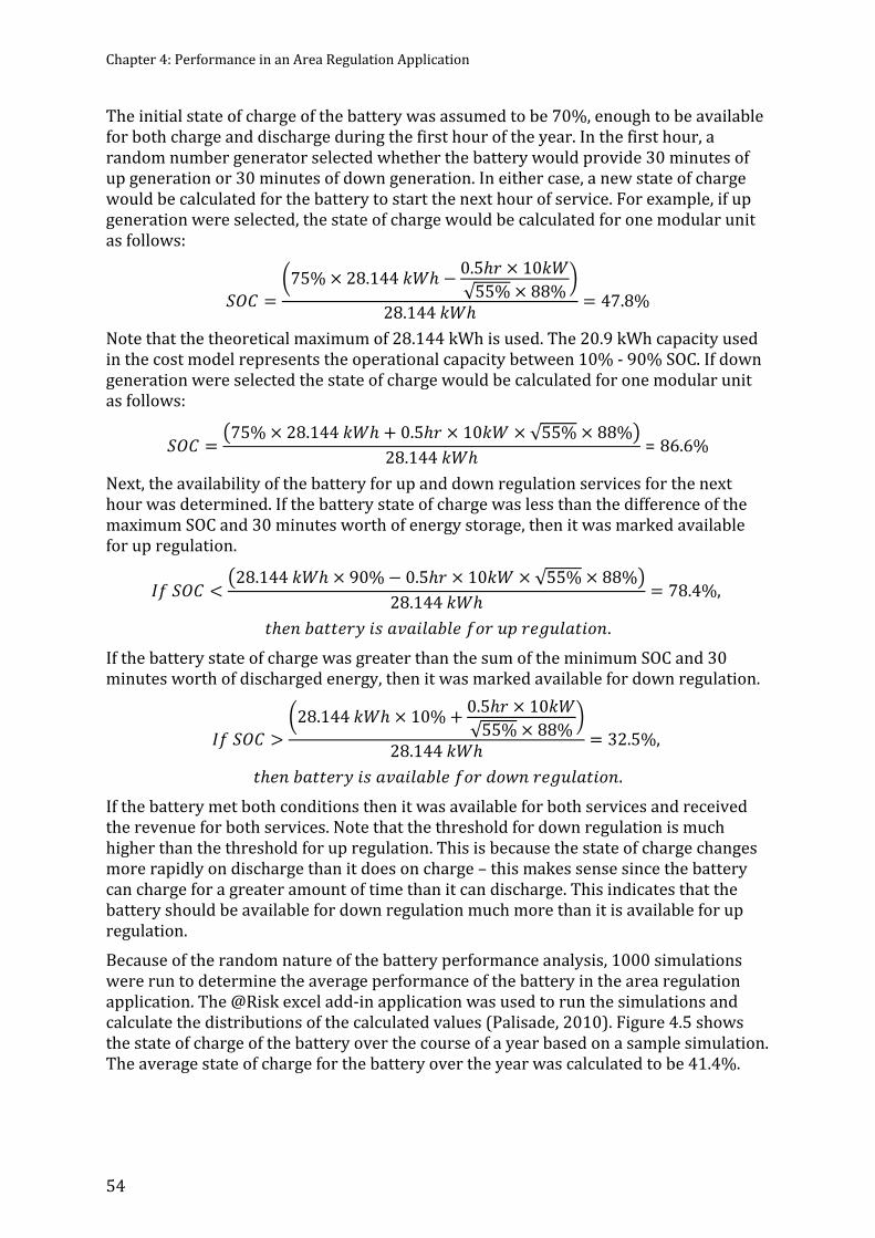
Chapter 4: Performance in an Area Regulation Application
54
The initial state of charge of the battery was assumed to be 70%, enough to be available for both charge and discharge during the first hour of the year. In the first hour, a random number generator selected whether the battery would provide 30 minutes of up generation or 30 minutes of down generation. In either case, a new state of charge would be calculated for the battery to start the next hour of service. For example, if up generation were selected, the state of charge would be calculated for one modular unit as follows: = 75% × 28.144 ℎ − 0.5ℎ × 10√55% × 88%28.144 ℎ = 47.8% Note that the theoretical maximum of 28.144 kWh is used. The 20.9 kWh capacity used in the cost model represents the operational capacity between 10% - 90% SOC. If down generation were selected the state of charge would be calculated for one modular unit as follows: = 75% × 28.144 ℎ + 0.5ℎ × 10 × √55% × 88%28.144 ℎ = 86.6% Next, the availability of the battery for up and down regulation services for the next hour was determined. If the battery state of charge was less than the difference of the maximum SOC and 30 minutes worth of energy storage, then it was marked available for up regulation. < 28.144 ℎ × 90% − 0.5ℎ × 10 × √55% × 88%28.144 ℎ = 78.4%, ℎ . If the battery state of charge was greater than the sum of the minimum SOC and 30 minutes worth of discharged energy, then it was marked available for down regulation.
> 28.144 ℎ × 10% + 0.5ℎ × 10√55% × 88%28.144 ℎ = 32.5%, ℎ . If the battery met both conditions then it was available for both services and received the revenue for both services. Note that the threshold for down regulation is much higher than the threshold for up regulation. This is because the state of charge changes more rapidly on discharge than it does on charge – this makes sense since the battery can charge for a greater amount of time than it can discharge. This indicates that the battery should be available for down regulation much more than it is available for up regulation. Because of the random nature of the battery performance analysis, 1000 simulations were run to determine the average performance of the battery in the area regulation application. The @Risk excel add-in application was used to run the simulations and calculate the distributions of the calculated values (Palisade, 2010). Figure 4.5 shows the state of charge of the battery over the course of a year based on a sample simulation. The average state of charge for the battery over the year was calculated to be 41.4%.

James Mellentine
55
Figure 4.5 – The state of charge of an iron hybrid flow battery over the course of a year in an area regulation
application. The average state of charge is 41.4%. The total number of charge & discharge cycles for the year was calculated by first calculating the amount of change in the SOC for each hour, and then summing the total percent change over the year. This quantity was divided by two to represent one full charge and discharge in a cycle. The average total number of cycles in a year was 714, which equals about 2 full cycles per day. The battery was available for up regulation 56.7% of the hours, while it was available for down regulation 96.9% of the hours. This result is in line with the expectations noted above. During the course of providing regulation services, the battery consumed an average of 6159 MWh from the grid, and sold back 2625 MWh. Based on 1000 simulations, the revenue generated from being available for regulation service was an average of $478,843. The distribution of revenues is presented in Figure 4.6. 90% of revenues fell between $472,280 and $485,604. If the battery were available 100% of all hours of the year, the maximum possible revenue was $609,441. The sales from the energy sold into the grid totaled $428,499, which when added to the revenue from regulation services equals an average total annual revenue of $907,342. However, the cost of the 6159 MWh purchased from the grid to provide those energy services was $1,005,928. When subtracted from the revenue, this represents a loss of $98,586/year. This doesn’t include maintenance costs and loan payments for the financing of such an installation, which would put the financial results further in the red. Also not considered in this analysis is the degradation in battery performance that is likely to happen over the life of the battery system. As the efficiencies dropped, the financial losses would get worse each year.
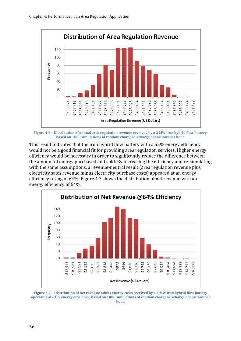
Chapter 4: Performance in an Area Regulation Application
56
Figure 4.6 – Distribution of annual area regulation revenue received by a 2 MW iron hybrid flow battery,
based on 1000 simulations of random charge/discharge operations per hour. This result indicates that the iron hybrid flow battery with a 55% energy efficiency would not be a good financial fit for providing area regulation services. Higher energy efficiency would be necessary in order to significantly reduce the difference between the amount of energy purchased and sold. By increasing the efficiency and re-simulating with the same assumptions, a revenue-neutral result (area regulation revenue plus electricity sales revenue minus electricity purchase costs) appeared at an energy efficiency rating of 64%. Figure 4.7 shows the distribution of net revenue with an energy efficiency of 64%.
Figure 4.7 – Distribution of net revenue minus energy costs received by a 2 MW iron hybrid flow battery
operating at 64% energy efficiency, based on 1000 simulations of random charge/discharge operations per hour.

James Mellentine
57
As the energy efficiency was increased further, the revenue increased accordingly. At an energy efficiency of 75%, the 2 MW iron hybrid flow battery would generate an average of $100,761 in net revenue per year. The distribution of net revenue for this scenario is shown in Figure 4.8. This energy efficiency level could serve as a future research target for the iron hybrid flow battery.
Figure 4.8 – Distribution of net revenue minus energy costs received by a 2 MW iron hybrid flow battery
operating at 75% energy efficiency, based on 1000 simulations of random charge/discharge operations per hour. A summary of performance results for the assumed 55% energy efficiency are presented in Table 4.3.
Table 4.3 – Summary of calculated performance metrics for a 2 MW iron hybrid flow battery performing in a hypothetical area regulation application at 55% energy efficiency.
Performance Characteristic Value Performance Characteristic Value Average up regulation price $14.89 Average SOC 41.4% Average down regulation price $17.32 Number cycles per year 714 Maximum possible revenue $609,441 Number cycles per day 2.0 Revenue earned from regulation $478,843 Up regulation availability 56.7%
Revenue earned from electricity sales $428,499 Down regulation availability 96.9% Cost of electricity purchased $1,005,928 Total electricity purchased 6159 MWh Net annual revenue -$98,586 Total electricity sold 2625 MWh

Chapter 4: Performance in an Area Regulation Application
58
1
1 In hindsight, the area regulation application may not have been the best choice to demonstrate financial viability of the iron hybrid flow battery. The authors of the referenced Sandia report somewhat arbitrarily doubled the monetary benefit of this application, which seems to have little/no basis for real operations in current markets. Thus, I did not make this same doubling assumption in my analysis. It is recommended that future work include analysis of the battery in other applications.

James Mellentine
59
Chapter 5: Laboratory Performance of an Iron Hybrid Flow Battery As a parallel effort to the design and cost model performed in an earlier chapter, a single-cell iron hybrid flow battery was cycled in the lab to measure its performance at varying current densities and plating densities. The details of the experiments, results, and comparisons with the assumed performance values in the cost model are described in this chapter. 5.1 Laboratory & Equipment This section describes the details of the lab station equipment and setup, the battery cell assembly, and electrolyte solution information. 5.1.1 The Test Station The lab station was located in the basement of the A.W. Smith building on the campus of Case Western Reserve University. It was a near-replica of other flow battery experimental stations used in the lab (the main difference being that the cell and tanks were placed inside an oven). Figure 5.1 shows a schematic of the lab station.
Figure 5.1 – A schematic diagram of the lab station used for the performance testing of an iron hybrid flow battery. Starting in the upper left corner of the diagram, there is a nitrogen tank. The purpose of the nitrogen is to provide a blanket of non-reactive gas over the electrolyte in an effort to prevent the oxidation of iron plate and ferrous ions. A tube from the nitrogen tank fed through a set of Porter Instruments F65 flow meters and into the tanks. The tank regulator valve was set at 20 psi (1.4 bar) and the flow meters were kept between 70-110 cm3/min – on the model A-125-5 used, this meant the float level was kept between 20 mm and 30 mm out of a maximum 65 mm (Porter, 2005). The nitrogen feed tube extended to the bottom of the electrolyte tanks and bubbled to the surface, providing a

Chapter 5: Laboratory Performance of an Iron Hybrid Flow Battery
60
continuous blanket over the electrolyte. The tank lids were not sealed tightly in order to provide a vent for the gases and avoid pressure build-up. Inside the oven, the battery cell and two tanks were stored at elevated temperatures to prevent precipitation of boric acid. For the initial tests using 1 M boric acid, the oven temperature was set to 60 ˚C. Later, the oven temperature was decreased to 45 ˚C in order to avoid deformation in the cell components. The oven temperature was controlled by a Cole Parmer temperature controller which measured the internal temperature with a thermocouple. Inside the oven, two 1-liter Nalgene polypropylene bottles were used as electrolyte tanks. According to the manufacturer these have a maximum service temperature of 104 ˚C (Nalgene Labware). The screw-top lids of the tanks have three ports that connect to tubes – one for the nitrogen feed described above, and one each for the electrolyte outlet and return. Also inside the oven was the battery cell. The battery is composed of several layers and will be shown in detail later in this chapter. Each side of the battery has an inlet and outlet for the electrolyte. As shown in the schematic, each side of the cell has a tube running from the tank outlet, through the pump, and to the battery inlet. Then another tube runs from the battery outlet to the tank return port. The latter tube between the battery outlet and the tank return was clear plastic, the purpose of which was to have the ability to observe gas evolution from the active cell area. Outside and above the oven, the electrolyte was pumped through each side of the cell using a Masterflex L/S peristaltic pump (model 77800-60). One drive motor powered two pumping attachments, one for each side of the cell. Thus each side of the cell had similar flow rates at any given time. The electrolyte was pumped through 17mm-diameter Masterflex Norprene tubing, which is rated up to 135 ˚C and has good resistance to acids (Masterflex). Moving to the right side of the schematic diagram, there was a desktop computer running LabVIEW software (National Instruments, 2010). Another researcher in the lab had previously developed a virtual interface (VI) control panel which was used in this study. The software was able to automatically control the power supply and load currents, switching functions between the power supply and load, and the pump flow rate. The VI also used time and voltage limits input by the user to automatically switch between charge and discharge (switching between the power supply and load). The VI also interfaced with a data acquisition unit that recorded voltage and current readings once per second and wrote the data to a text data file. As shown in the diagram, the computer was connected to pump and switch controls along with a data acquisition unit. The pump and switch controls were essentially a breadboard spliced with an integrated circuit board which was connected to the computer via a universal serial bus (USB) port. The controls were connected to the two-way switching unit that switched between the power supply and load. They were also connected to the pump via a data cable to control the pump flow rate. The data acquisition unit was an Agilent Technologies 34970A. One set of electrical leads traversed from the battery terminals to the data acquisition unit to supply voltage readings. Another set of electrical leads traversed from the shunt to the data acquisition unit to supply current readings. These readings were taken once per second during charge and discharge and recorded in a text file.

James Mellentine
61
To the left of the computer in the schematic diagram is the power supply and electronic load. The power supply was an Amrel SPS20-60-0020. This was used to provide current to the battery during charge operations. The electronic load was originally an Amrel FEL60-1, but was later switched to an Amrel ZVL200-150-40L in an effort to obtain lower discharge voltages. The positive and negative cables from both the power supply and load were connected to the two-way switch, with one each positive and negative cable from the switch being connected to the battery terminals. This allowed an easy transition between charge and discharge operations without manually switching cables back and forth. On the negative cable running from the switch to the battery was a shunt rated up to 20 A at 50 mV, which equates to a resistance of 2.5 mΩ. The known resistance of this shunt was used to measure the current using leads connected to the data acquisition unit. 5.1.2 The Single-Cell Battery Assembly The battery cell itself was composed of several layers. The layers are shown in Figure 5.2.
Figure 5.2 – Photograph of 50 cm2 cell used for experiments. The left photo is the assembled cell with all
layers. The smaller right-side photos are cross-sectional views of each layer. The numbered labels correspond to: 1) Flow block, 2) Non-conducting Teflon layer, 3) Gold-plated copper conductor, 4) Grafoil
layer 5) Graphite electrode, 6) PVC spacer & activated felt layer, 7) Membrane, 8) Negative electrolyte inlet, and 9) Positive electrolyte outlet. Layer 1 was a thick polyvinylchloride (PVC) flow block. This block has inlet and outlet ports for the flowing electrolyte. Layer 2 was a thin and flexible Teflon layer that provides a compressible “seat” for the copper collector plate. Note that this layer has holes aligned with the flow holes (lower left and upper right corners) to allow electrolyte to flow through. Layer 3 was the gold-plated copper collector plate, with a terminal protruding upward. This plate also has holes aligned with the flow. To provide a good seal around this flow, small Viton rubber gaskets are fitted into each of the holes in the copper plate (the figure is shown with the rubber gaskets in place).
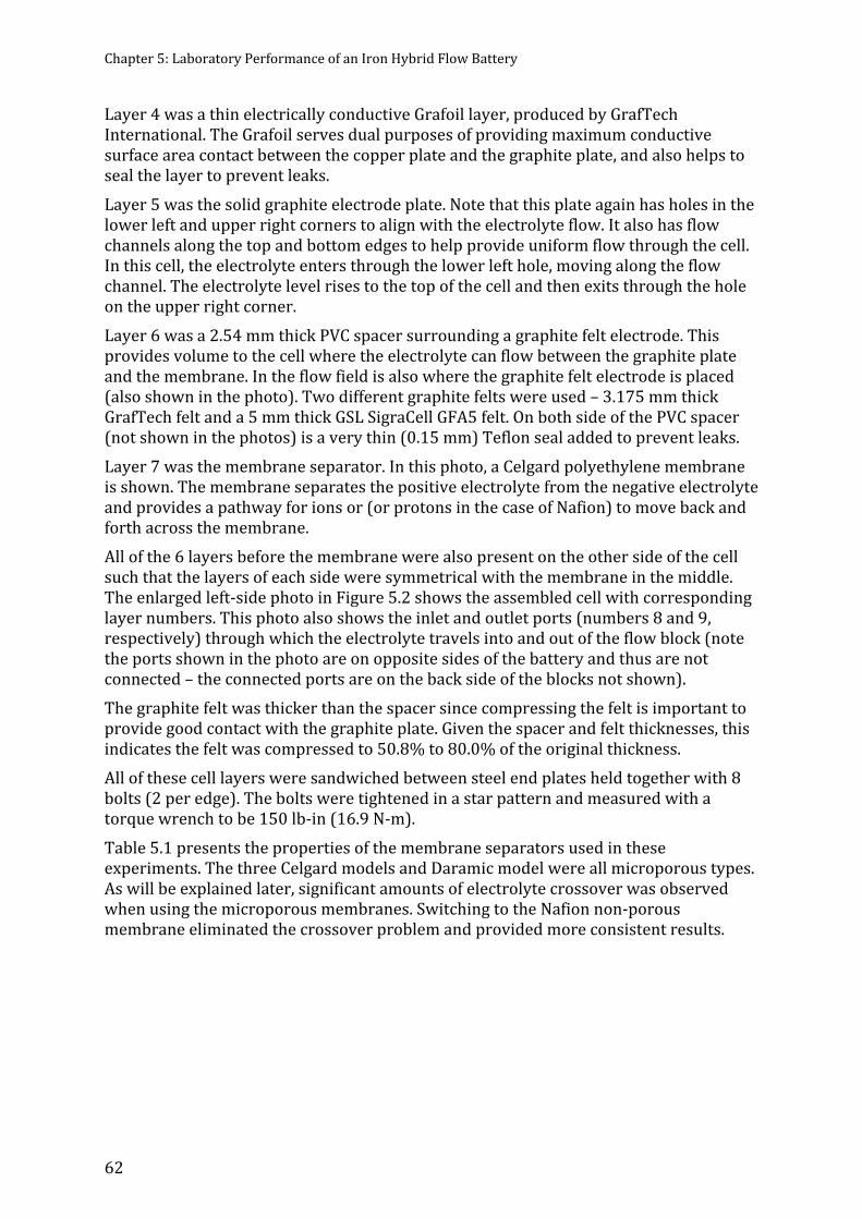
Chapter 5: Laboratory Performance of an Iron Hybrid Flow Battery
62
Layer 4 was a thin electrically conductive Grafoil layer, produced by GrafTech International. The Grafoil serves dual purposes of providing maximum conductive surface area contact between the copper plate and the graphite plate, and also helps to seal the layer to prevent leaks. Layer 5 was the solid graphite electrode plate. Note that this plate again has holes in the lower left and upper right corners to align with the electrolyte flow. It also has flow channels along the top and bottom edges to help provide uniform flow through the cell. In this cell, the electrolyte enters through the lower left hole, moving along the flow channel. The electrolyte level rises to the top of the cell and then exits through the hole on the upper right corner. Layer 6 was a 2.54 mm thick PVC spacer surrounding a graphite felt electrode. This provides volume to the cell where the electrolyte can flow between the graphite plate and the membrane. In the flow field is also where the graphite felt electrode is placed (also shown in the photo). Two different graphite felts were used – 3.175 mm thick GrafTech felt and a 5 mm thick GSL SigraCell GFA5 felt. On both side of the PVC spacer (not shown in the photos) is a very thin (0.15 mm) Teflon seal added to prevent leaks. Layer 7 was the membrane separator. In this photo, a Celgard polyethylene membrane is shown. The membrane separates the positive electrolyte from the negative electrolyte and provides a pathway for ions or (or protons in the case of Nafion) to move back and forth across the membrane. All of the 6 layers before the membrane were also present on the other side of the cell such that the layers of each side were symmetrical with the membrane in the middle. The enlarged left-side photo in Figure 5.2 shows the assembled cell with corresponding layer numbers. This photo also shows the inlet and outlet ports (numbers 8 and 9, respectively) through which the electrolyte travels into and out of the flow block (note the ports shown in the photo are on opposite sides of the battery and thus are not connected – the connected ports are on the back side of the blocks not shown). The graphite felt was thicker than the spacer since compressing the felt is important to provide good contact with the graphite plate. Given the spacer and felt thicknesses, this indicates the felt was compressed to 50.8% to 80.0% of the original thickness. All of these cell layers were sandwiched between steel end plates held together with 8 bolts (2 per edge). The bolts were tightened in a star pattern and measured with a torque wrench to be 150 lb-in (16.9 N-m). Table 5.1 presents the properties of the membrane separators used in these experiments. The three Celgard models and Daramic model were all microporous types. As will be explained later, significant amounts of electrolyte crossover was observed when using the microporous membranes. Switching to the Nafion non-porous membrane eliminated the crossover problem and provided more consistent results.

James Mellentine
63
Table 5.1 – The general physical properties of the six membrane separator materials that were used in the course of experiments with an iron hybrid flow battery (Celgard, 2010) (Daramic, 2000).
Separator Material Thickness Porosity Pore Size
Gurley Porosity
Puncture Strength Celgard 3401 Monolayer Polypropylene 25 μm 41% 0.043 μm 620 seconds 450 g
Celgard 3501 Monolayer Polypropylene 25 μm 55% 0.064 μm 200 seconds 335 g Celgard 5550 Monolayer Polypropylene laminated to non-woven fabric 110 μm with laminate, 25 μm without laminate 55% 0.064 μm 200 seconds 335 g Daramic Polyethylene with amorphous silica 254 μm 58% (no data) (no data) 7.5 N Nafion 1035 Sulfonated tetrafluoroethylene 0.009 cm (dry) 0% 0 N/A (no data) Nafion 1135 Sulfonated tetrafluoroethylene 0.018 cm (dry) 0% 0 N/A (no data)
5.1.3 Electrolyte Solutions The electrolyte solutions used in these experiments were prepared using nanopure de-ionized (DI) water measuring 18.2 MΩ-cm resistance. All other chemicals were ACS-grade or higher. Electrolytes were prepared in standard laboratory glassware. Chemicals were weighed in weighing dishes on digital scales. Solutions were mixed and heated on heated magnetic stirring plates. Acidity measurements were taken for each electrolyte solution using a digital pH meter. Details on electrolyte preparation are included in the next section. 5.2 Data Collection Methodology This section describes the method for preparing electrolyte, cycling the battery, and calculating results. 5.2.1 Electrolyte Preparation Electrolyte solutions were prepared by first heating DI water to about 50-60 ˚C in a volumetric flask about 2/3 full on a heated magnetic stirrer. Once sufficiently heated, the boric acid was weighed on a digital scale and added to the flask. This was added first since it took the longest to dissolve, and complete dissolution indicated the temperature of the solution was warm enough. Next the supporting electrolyte (either NH4Cl or NaCl depending on the experiment) was weighed on a digital scale and added to the solution. This electrolyte was completely dissolved before finally adding the ferrous chloride.

Chapter 5: Laboratory Performance of an Iron Hybrid Flow Battery
64
The ferrous chloride was weighed and added to the solution last. Additional DI water was added to the flask until the volume of the solution rose to the indicated line on the volumetric flask. Electrolyte batches were usually prepared in two separate flasks (one 1000 mL and one 500 mL) and then mixed together before taking a pH reading and transferring to the electrolyte tanks. 5.2.2 Cycling the Battery Before commencing data collection on the full battery, the positive electrode behavior was confirmed by cycling the cell with a positive electrolyte mixture on both sides of the cell. In other words, a solution with both ferric (Fe3+) and ferrous (Fe2+) ions was prepared to mimic the chemistry on the positive side of a partially-charged battery. This was accomplished by adding ferrous chloride and ferric chloride instead of just ferrous chloride. The purpose of this test was to observe the voltage behavior of this “symmetric” cell and confirm its stability and reproducibility before moving to the regular chemistry of the iron hybrid flow battery. It was suspected that performance problems in the iron hybrid flow cell would come from the negative side, where the plating reaction occurs. That could be confirmed in future tests if the positive-side reaction was found to be stable and predictable. Charge and discharge operations on the symmetric cell simply increased and decreased the concentration of the ferric and ferrous ions on each side, without the occurrence of plating behavior. Because the reaction potential is essentially the same on both sides of the symmetric cell, the battery did not store enough energy to be able to discharge using the electronic load. Therefore, the leads on the power supply were simply reversed to cycle the battery in the opposite direction. For these tests when the leads were reversed the voltage data was recorded as negative and was subsequently multiplied by -1 before graphing the results. The symmetric cell was initially conducted with the Celgard 5550 membrane material with NH4Cl used as the supporting electrolyte. Six cycles were conducted on the symmetric cell at a current density of 50 mA/cm2, and six cycles were conducted at a current density of 100 mA/cm2. After the decision was made to move to the non-porous membrane (to prevent electrolyte crossover), the symmetric cell tests were conducted again, this time with the Nafion membrane material and NaCl as the supporting electrolyte. This set of tests included six cycles at each current density and include current densities of 50 mA/cm2, 100 mA/cm2, 200 mA/cm2, 300 mA/cm2, and 400 mA/cm2. Table 5.2 shows a summary of symmetric cell test settings.

James Mellentine
65
Table 5.2 – The cycles are shown for the symmetric cell tests, along with current density and pump flow rate for each cycle. Cycles 1-13 were conducted with microporous membrane. Cycles 31-68 were conducted with Nafion membrane.
Cycle #
Current Density (mA/cm2)
Pump Flow Rate (mL/min)
Cycle #
Current Density (mA/cm2)
Pump Flow Rate (mL/min) 1 50 48.6 44 50 48.6 2 50 48.6 45 100 97.2 3 50 48.6 46 100 97.2 4 50 48.6 47 100 97.2 5 50 48.6 48 100 97.2 6 50 48.6 49 100 97.2 7 50 48.6 50 100 97.2 8 100 97.2 51 200 194.3 9 100 97.2 52 200 194.3 10 100 97.2 53 200 194.3 11 100 97.2 54 200 194.3 12 100 97.2 55 200 194.3 13 100 97.2 56 200 194.3 31 50 48.6 57 300 291.5 32 50 48.6 58 300 291.5 33 50 48.6 59 300 291.5 34 50 48.6 60 300 291.5 35 50 48.6 61 300 291.5 36 50 48.6 62 300 291.5 37 50 48.6 63 400 388.7 38 100 97.2 64 400 388.7 39 50 48.6 65 400 388.7 40 50 48.6 66 400 388.7 41 50 48.6 67 400 388.7 42 50 48.6 68 400 388.7 43 50 48.6 After the symmetric cell tests, the electrolyte solution was replaced with the regular all-ferrous ion solution to conduct the performance tests. The current density, charge time, discharge time, pump flow rate, and voltage limits were entered into the VI control for each cycle and the data was output to data files. Observations regarding electrolyte crossover, gas evolution, and cell leakage were noted when present. As discussed in a later section, it was a challenge to get the battery to properly function in early testing cycles. There was significant crossover of electrolyte from one tank to another, and the battery would not effectively charge or discharge on a consistent basis. Some of the problems that caused these poor results are unknown, and the overall performance is contrary to the more consistent performance shown in a previous study
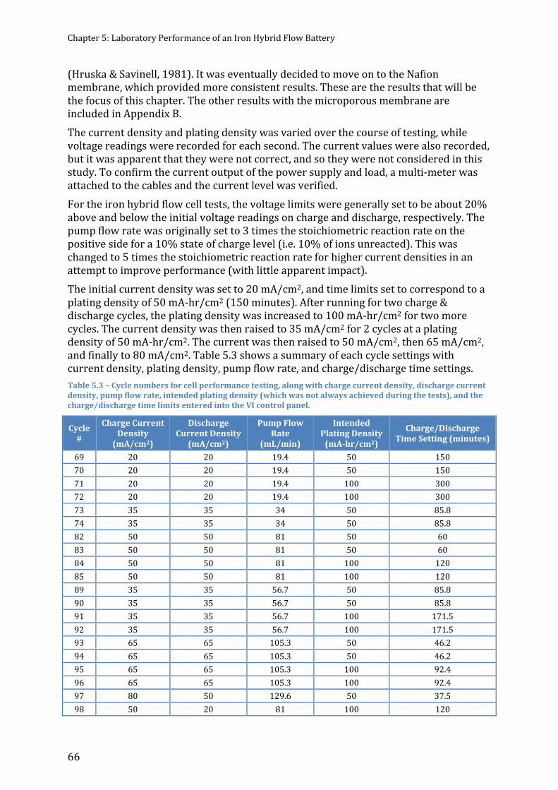
Chapter 5: Laboratory Performance of an Iron Hybrid Flow Battery
66
(Hruska & Savinell, 1981). It was eventually decided to move on to the Nafion membrane, which provided more consistent results. These are the results that will be the focus of this chapter. The other results with the microporous membrane are included in Appendix B. The current density and plating density was varied over the course of testing, while voltage readings were recorded for each second. The current values were also recorded, but it was apparent that they were not correct, and so they were not considered in this study. To confirm the current output of the power supply and load, a multi-meter was attached to the cables and the current level was verified. For the iron hybrid flow cell tests, the voltage limits were generally set to be about 20% above and below the initial voltage readings on charge and discharge, respectively. The pump flow rate was originally set to 3 times the stoichiometric reaction rate on the positive side for a 10% state of charge level (i.e. 10% of ions unreacted). This was changed to 5 times the stoichiometric reaction rate for higher current densities in an attempt to improve performance (with little apparent impact). The initial current density was set to 20 mA/cm2, and time limits set to correspond to a plating density of 50 mA-hr/cm2 (150 minutes). After running for two charge & discharge cycles, the plating density was increased to 100 mA-hr/cm2 for two more cycles. The current density was then raised to 35 mA/cm2 for 2 cycles at a plating density of 50 mA-hr/cm2. The current was then raised to 50 mA/cm2, then 65 mA/cm2, and finally to 80 mA/cm2. Table 5.3 shows a summary of each cycle settings with current density, plating density, pump flow rate, and charge/discharge time settings. Table 5.3 – Cycle numbers for cell performance testing, along with charge current density, discharge current density, pump flow rate, intended plating density (which was not always achieved during the tests), and the charge/discharge time limits entered into the VI control panel.
Cycle #
Charge Current Density
(mA/cm2)
Discharge Current Density
(mA/cm2)
Pump Flow Rate
(mL/min)
Intended Plating Density
(mA-hr/cm2)
Charge/Discharge Time Setting (minutes) 69 20 20 19.4 50 150 70 20 20 19.4 50 150 71 20 20 19.4 100 300 72 20 20 19.4 100 300 73 35 35 34 50 85.8 74 35 35 34 50 85.8 82 50 50 81 50 60 83 50 50 81 50 60 84 50 50 81 100 120 85 50 50 81 100 120 89 35 35 56.7 50 85.8 90 35 35 56.7 50 85.8 91 35 35 56.7 100 171.5 92 35 35 56.7 100 171.5 93 65 65 105.3 50 46.2 94 65 65 105.3 50 46.2 95 65 65 105.3 100 92.4 96 65 65 105.3 100 92.4 97 80 50 129.6 50 37.5 98 50 20 81 100 120
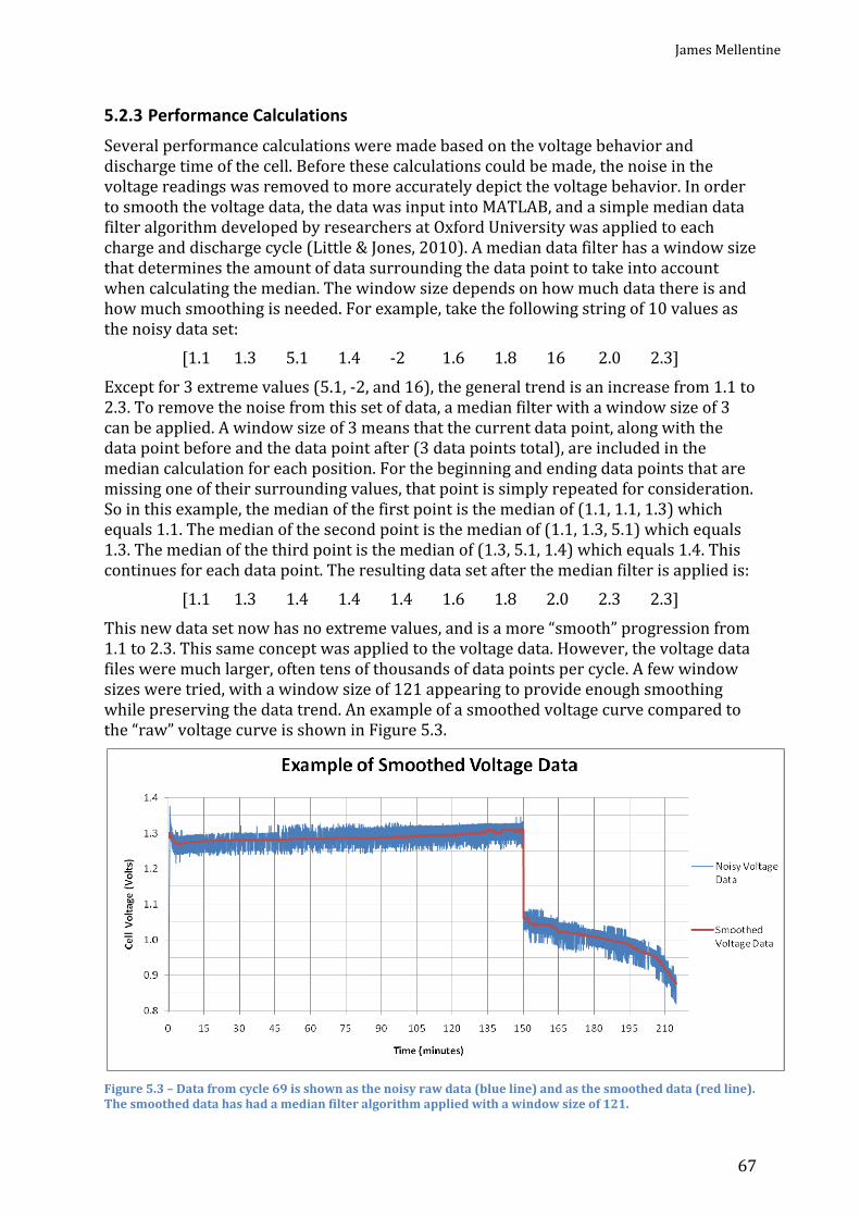
James Mellentine
67
5.2.3 Performance Calculations Several performance calculations were made based on the voltage behavior and discharge time of the cell. Before these calculations could be made, the noise in the voltage readings was removed to more accurately depict the voltage behavior. In order to smooth the voltage data, the data was input into MATLAB, and a simple median data filter algorithm developed by researchers at Oxford University was applied to each charge and discharge cycle (Little & Jones, 2010). A median data filter has a window size that determines the amount of data surrounding the data point to take into account when calculating the median. The window size depends on how much data there is and how much smoothing is needed. For example, take the following string of 10 values as the noisy data set: [1.1 1.3 5.1 1.4 -2 1.6 1.8 16 2.0 2.3] Except for 3 extreme values (5.1, -2, and 16), the general trend is an increase from 1.1 to 2.3. To remove the noise from this set of data, a median filter with a window size of 3 can be applied. A window size of 3 means that the current data point, along with the data point before and the data point after (3 data points total), are included in the median calculation for each position. For the beginning and ending data points that are missing one of their surrounding values, that point is simply repeated for consideration. So in this example, the median of the first point is the median of (1.1, 1.1, 1.3) which equals 1.1. The median of the second point is the median of (1.1, 1.3, 5.1) which equals 1.3. The median of the third point is the median of (1.3, 5.1, 1.4) which equals 1.4. This continues for each data point. The resulting data set after the median filter is applied is: [1.1 1.3 1.4 1.4 1.4 1.6 1.8 2.0 2.3 2.3] This new data set now has no extreme values, and is a more “smooth” progression from 1.1 to 2.3. This same concept was applied to the voltage data. However, the voltage data files were much larger, often tens of thousands of data points per cycle. A few window sizes were tried, with a window size of 121 appearing to provide enough smoothing while preserving the data trend. An example of a smoothed voltage curve compared to the “raw” voltage curve is shown in Figure 5.3.
Figure 5.3 – Data from cycle 69 is shown as the noisy raw data (blue line) and as the smoothed data (red line). The smoothed data has had a median filter algorithm applied with a window size of 121.

Chapter 5: Laboratory Performance of an Iron Hybrid Flow Battery
68
After the voltage data was smoothed, the first performance calculation was the nominal charge and discharge voltage. The nominal charge voltage was calculated as the average of all voltage readings on the charge cycle. Likewise with the nominal discharge voltage being the average of all voltage readings on the discharge cycle. The voltaic efficiency was then calculated as simply the ratio of the discharge voltage over the charge voltage. = ℎ ℎ The coulombic efficiency was the next calculated value. Coulombic efficiency is a equal to the amount of charge (coulombs) that come out of the battery on the discharge operation divided by the amount of charge that was forced into the battery during the charge operation. Charge is the product of current and time. Since the current was the same on charge and discharge, the current value simply drops out and the efficiency becomes the ratio of the discharge time divided by the charge time. = ℎ × ℎ ℎ × ℎ = ℎ ℎ The round-trip energy efficiency of the battery is the product of the voltaic and coulombic efficiencies. = × The nominal power on discharge was calculated as the product of the discharge current and the nominal discharge voltage. = ℎ × ℎ The power density was calculated as the nominal power divided by the active cell area. = The energy capacity was calculated as the product of the nominal power and the discharge time. = × ℎ The specific energy was calculated per mass of iron plated onto the electrode by dividing the energy capacity by mass of plate. = × × × ℎ = The percent of reactant utilization was also calculated. It is not the intent of this study to maximize the amount of reactants utilized in each cycle, however it is still interesting to determine this to see what amount of reactant was used compared to the theoretical maximum. For the iron hybrid flow battery, the reactant utilization was limited by the plating density on the negative side (discussed further in another section). The percent of reactant utilization can be calculated as the ratio of the actual plating density divided by the maximum theoretical plating density.

James Mellentine
69
= × × × ℎ = 5.3 Experimental Results This section describes the results obtained from cycling the single-cell iron hybrid flow battery. Included are details about the electrolyte solutions, results from the symmetric cell tests, results from the iron hybrid flow cell tests, and performance calculations. At the end these performance calculations are compared to the assumptions made for the cost model discussed in a previous chapter. 5.3.1 Electrolyte Solution Data The electrolyte solutions used in this study had a tendency to deteriorate relatively quickly, usually within less than 7 cycles (except for the symmetric cell tests). After several charge and discharge cycles, the voltage behavior became more erratic and higher overvoltages were required for charge and discharge operations, sometimes so large that the load could not maintain a constant current on discharge. Changing the electrolyte (along with other adjustments like acid washing the Nafion membrane) would generally improve the battery performance. Out of the 47 charge and discharge cycles conducted (not counting symmetric cell tests), 13 electrolyte batches were used – that’s an average of 3.6 cycles per batch. The performance results in this section will focus on the results obtained from the symmetric cell tests that used the microporous membrane as well as the symmetric and iron hybrid flow cell tests that used the non-porous membrane. Table 5.4 shows the electrolyte solution batch numbers and properties that correspond to the various cycle numbers in this study. It should also be noted that before cycle number 69, a different concentration of ferrous chloride was being used than intended, due to the misidentification of the ferrous chloride as the anhydrous form, whereas it was actually tetrahydrate. The first electrolyte batch was used for the symmetric cell tests with the Celgard 5550 microporous membrane (cycles 1-13). Electrolyte batches 2-7 (corresponding to cycles 14-30) are not listed in this table, but are included in Appendix B. These cycles represent data from the cell early in the study when the battery was not always functioning as expected and troubleshooting was occurring, and thus are not in the focus of the results of the study. Electrolyte batches 8, 9, and 10 were used in the first attempts to conduct the symmetric cell tests with the non-porous membrane. It was apparent that the voltage behavior was not as expected and after a review of the literature it was found that ammonium ions are not compatible with Nafion membranes. The supporting electrolyte salt was thus changes to NaCl in batch 11, which was used throughout the 30 symmetric cell charge cycles with steady and repeatable results.
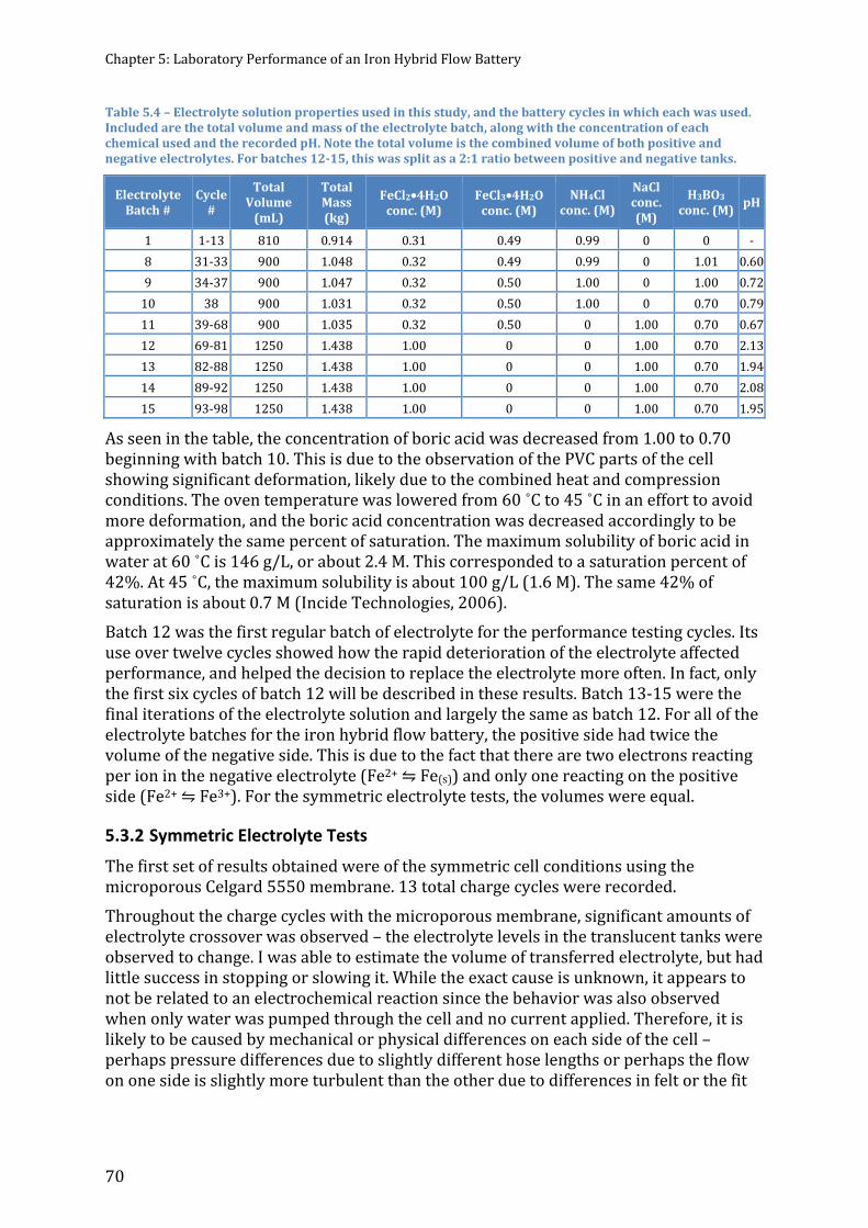
Chapter 5: Laboratory Performance of an Iron Hybrid Flow Battery
70
Table 5.4 – Electrolyte solution properties used in this study, and the battery cycles in which each was used. Included are the total volume and mass of the electrolyte batch, along with the concentration of each chemical used and the recorded pH. Note the total volume is the combined volume of both positive and negative electrolytes. For batches 12-15, this was split as a 2:1 ratio between positive and negative tanks.
Electrolyte Batch #
Cycle #
Total Volume
(mL)
Total Mass (kg)
FeCl2•4H2O conc. (M)
FeCl3•4H2O conc. (M)
NH4Cl conc. (M)
NaCl conc. (M)
H3BO3 conc. (M) pH
1 1-13 810 0.914 0.31 0.49 0.99 0 0 - 8 31-33 900 1.048 0.32 0.49 0.99 0 1.01 0.609 34-37 900 1.047 0.32 0.50 1.00 0 1.00 0.7210 38 900 1.031 0.32 0.50 1.00 0 0.70 0.7911 39-68 900 1.035 0.32 0.50 0 1.00 0.70 0.6712 69-81 1250 1.438 1.00 0 0 1.00 0.70 2.1313 82-88 1250 1.438 1.00 0 0 1.00 0.70 1.9414 89-92 1250 1.438 1.00 0 0 1.00 0.70 2.0815 93-98 1250 1.438 1.00 0 0 1.00 0.70 1.95As seen in the table, the concentration of boric acid was decreased from 1.00 to 0.70 beginning with batch 10. This is due to the observation of the PVC parts of the cell showing significant deformation, likely due to the combined heat and compression conditions. The oven temperature was lowered from 60 ˚C to 45 ˚C in an effort to avoid more deformation, and the boric acid concentration was decreased accordingly to be approximately the same percent of saturation. The maximum solubility of boric acid in water at 60 ˚C is 146 g/L, or about 2.4 M. This corresponded to a saturation percent of 42%. At 45 ˚C, the maximum solubility is about 100 g/L (1.6 M). The same 42% of saturation is about 0.7 M (Incide Technologies, 2006). Batch 12 was the first regular batch of electrolyte for the performance testing cycles. Its use over twelve cycles showed how the rapid deterioration of the electrolyte affected performance, and helped the decision to replace the electrolyte more often. In fact, only the first six cycles of batch 12 will be described in these results. Batch 13-15 were the final iterations of the electrolyte solution and largely the same as batch 12. For all of the electrolyte batches for the iron hybrid flow battery, the positive side had twice the volume of the negative side. This is due to the fact that there are two electrons reacting per ion in the negative electrolyte (Fe2+ ⇋ Fe(s)) and only one reacting on the positive side (Fe2+ ⇋ Fe3+). For the symmetric electrolyte tests, the volumes were equal. 5.3.2 Symmetric Electrolyte Tests The first set of results obtained were of the symmetric cell conditions using the microporous Celgard 5550 membrane. 13 total charge cycles were recorded. Throughout the charge cycles with the microporous membrane, significant amounts of electrolyte crossover was observed – the electrolyte levels in the translucent tanks were observed to change. I was able to estimate the volume of transferred electrolyte, but had little success in stopping or slowing it. While the exact cause is unknown, it appears to not be related to an electrochemical reaction since the behavior was also observed when only water was pumped through the cell and no current applied. Therefore, it is likely to be caused by mechanical or physical differences on each side of the cell – perhaps pressure differences due to slightly different hose lengths or perhaps the flow on one side is slightly more turbulent than the other due to differences in felt or the fit

James Mellentine
71
of the cell layers. It is also possible that there are small punctures in the membrane itself, although none were observed on the membrane from these first 13 cycles.
Figure 5.4 – The estimated electrolyte crossover rate observed during symmetric cell tests using the
microporous membrane. Positive rates indicate electrolyte transfer from the rear tank to the front tanks. Negative rates indicate the opposite, electrolyte transferring from the front tank to the rear tank. Note that for the symmetric cell experiments, the voltage values are the cell voltage. Since the ferric/ferrous ion concentrations start out being the same on both sides of the cell, the open circuit cell voltage should be zero and the voltage with current applied is the overvoltage. Then as the concentrations change, the open circuit voltage also changes, and the cell voltage is the sum of the open circuit voltage and the overvoltages at each electrode. The estimated change in the equilibrium (open circuit) voltage between the extremes of the cycle can be calculated from the Nernst equation: = [ 2+][ 2+] Where: R = universal gas constant T = cell temperature z = charge ratio F = Faraday constant [Fe2+]P = concentration of ferrous ion in the positive half-cell [Fe2+]N = concentration of ferrous ion in the negative half-cell In this specific electrolyte batch, the concentration of ferrous ion will theoretically vary between 0 M and 0.8 M on each side of the symmetric cell. This means the open circuit potential will vary between -0.12 V and 0.12 V through a single charge cycle, with an open circuit potential of zero occurring when there are 0.4 M of ferrous ions on each side of the cell. Figure 5.5 shows a graph of this potential throughout the possible range of concentrations in the cell. This potential range holds for all symmetric cell tests

Chapter 5: Laboratory Performance of an Iron Hybrid Flow Battery
72
discussed in this section. In comparison to the overall cell voltages measured, the open circuit potential is less than half of the cell voltage.
Figure 5.5 – Theoretical open circuit (equilibrium) potential of the symmetric cell. The first seven charge cycles were conducted at a current density of 50 mA/cm2. The goal of the symmetric cell test was to observe the voltage behavior across several cycles, so the voltage limits and time limits were not restrictive. Since there are 0.324 moles of iron ions on each side of the battery, the maximum theoretical charge time can be calculated by multiplying by the Faraday constant (26.8 A-hr/mol) and dividing by the current (2.5 A). In this case, a full charge has a maximum of 208.4 minutes. The voltage curves from these first 7 cycles are shown in Figure 5.6.
Figure 5.6 – Voltage curves from the symmetric cell cycles 1-7 using the Celgard 5550 PP membrane and
NH4Cl as the supporting electrolyte salt, and a current density of 50 mA/cm2.

James Mellentine
73
The first cycle is only about half as long as the other cycles since it started from the mixed ferrous/ferric solution. The outlying cycle 4 is the result of being “re-charged” after cycle 3. Since so much electrolyte solution had crossed over to one side of the cell during cycle 3, some of the electrolyte from the front tank was poured into the rear tank after cycle 3 to equalize the volumes, and then re-charged into order to drive all of the ions back to the charged state. The remaining cycles are very consistent and repeatable through about 150 minutes, at when time the voltage starts to rise significantly (indicating most of the ions that are available for reaction have reacted). After the steep rise in the cell voltage, it began to level off again in the range of 1.0-1.5 V. This is likely due to an evolving of oxygen after the reactants were mostly used up. This is not an important part of the data, so it is helpful to view a close-up of this data to confirm the consistent behavior. Figure 5.7 shows a zoomed view of these cycles with a smaller time and voltage range, and removing the first half-charge cycle 1 and outlying re-charge cycle 4. This view confirms the consistency and repeatability of the ferrous/ferric ion reaction in the positive electrolyte. The cell voltage begins below 0.04 volts and steadily rises to between 0.175 and 0.200 volts at 150 minutes, after which time the cell voltage starts to rise more rapidly. At 50 mA/cm2, the percent of theoretical maximum charge limit ranged between 77% to 91% before the rapid rise in voltage.
Figure 5.7 – A zoomed view of the voltage curves from cycles 2, 3, 5, 6, and 7. The voltage behavior shows
consistency and repeatability through about 150 minutes at 50 mA/cm2. Cycles 8-13 were conducted at a current density of 100 mA/cm2. Again, the voltage limits and time limits were not restrictive. The voltage curves from these cycles are shown in Figure 5.8. The maximum theoretical charge time was 104.2 minutes.

Chapter 5: Laboratory Performance of an Iron Hybrid Flow Battery
74
Figure 5.8 – Voltage curves from the symmetric cell cycles 8-13 using the Celgard 5550 PP membrane and
NH4Cl as the supporting electrolyte salt, and a current density of 100 mA/cm2. All cycles in this graph were full charge cycles. Cycle 8 appears to be an outlier, with a higher cell voltage and shorter charge time than the others. The remaining cycles are very consistent and repeatable through about 75 minutes, at which time the voltage starts to rise significantly (indicating most of the ions that are available for reaction have reacted). It is helpful to view a close-up of this data to confirm the consistent behavior. Figure 5.9 shows a zoomed view of these cycles with a smaller time and voltage range. This view confirms the consistency and repeatability of the ferrous/ferric ion reaction in the positive electrolyte. The cell voltage begins between 0.10-0.17 volts and (except for cycle 8) steadily rises to between 0.275 and 0.325 volts at 75 minutes, after which time the cell voltage starts to rise more rapidly. This higher voltage and shorter charge time is expected since the current is doubled. At 100 mA/cm2, the percent of theoretical maximum charge limit (not counting outlying cycle 8) ranged between 75% to 81% before the rapid rise in voltage.
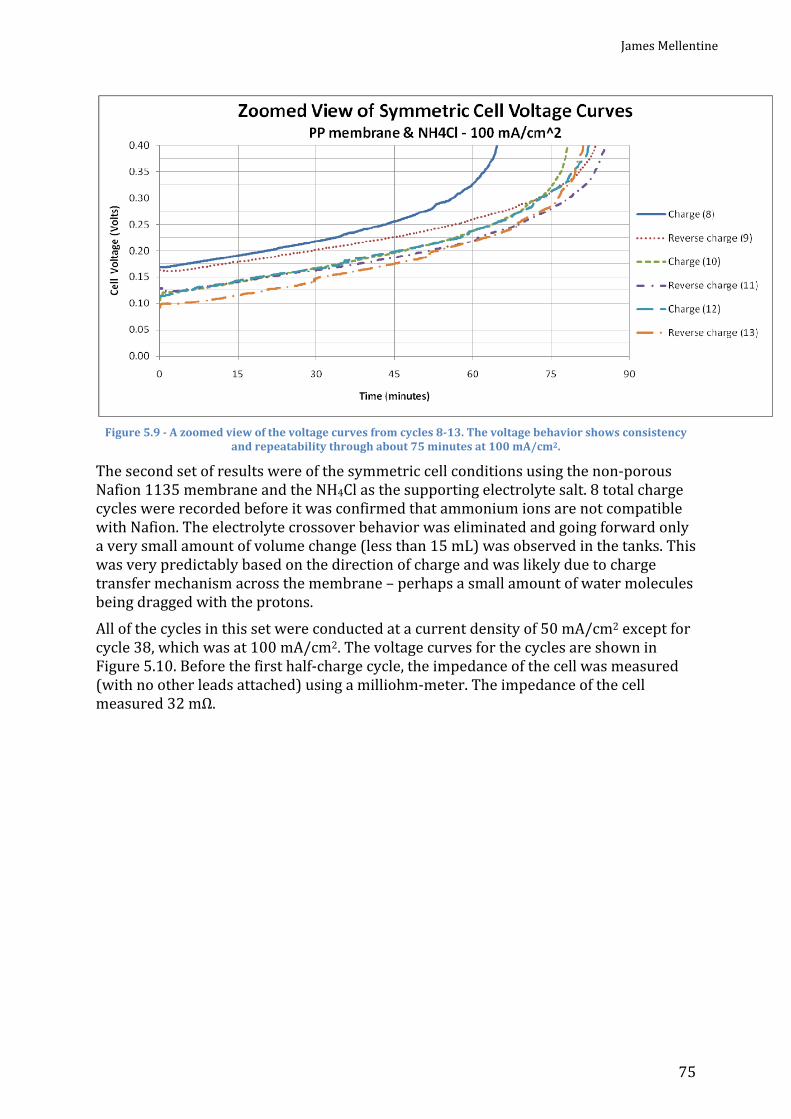
James Mellentine
75
Figure 5.9 - A zoomed view of the voltage curves from cycles 8-13. The voltage behavior shows consistency
and repeatability through about 75 minutes at 100 mA/cm2. The second set of results were of the symmetric cell conditions using the non-porous Nafion 1135 membrane and the NH4Cl as the supporting electrolyte salt. 8 total charge cycles were recorded before it was confirmed that ammonium ions are not compatible with Nafion. The electrolyte crossover behavior was eliminated and going forward only a very small amount of volume change (less than 15 mL) was observed in the tanks. This was very predictably based on the direction of charge and was likely due to charge transfer mechanism across the membrane – perhaps a small amount of water molecules being dragged with the protons. All of the cycles in this set were conducted at a current density of 50 mA/cm2 except for cycle 38, which was at 100 mA/cm2. The voltage curves for the cycles are shown in Figure 5.10. Before the first half-charge cycle, the impedance of the cell was measured (with no other leads attached) using a milliohm-meter. The impedance of the cell measured 32 mΩ.

Chapter 5: Laboratory Performance of an Iron Hybrid Flow Battery
76
Figure 5.10 - Voltage curves from symmetric cell cycles 31-38 using the Nafion 1135 membrane and NH4Cl as
the supporting electrolyte salt. The current density was 50 mA/cm2. Marked deterioration in performance was observed starting with cycle 34. The first three charge cycles (cycles 31-33) exhibited steady voltage behavior with a similar shape as the first set of symmetric cell tests, except with a shorter charge time. The impedance of the cell was again measured after cycle 32 and again had the same measurement of 32 mΩ. However, after cycle 33, the inlet tube leading to one of the flow blocks burst from the block due to high system pressure, and most of the electrolyte from that tank was spilled. A new batch of electrolyte was mixed before cycle 34. A new impedance measurement with the new electrolyte showed an increase to 46 mΩ. Cycle 34 is another half-charge, and the voltage climbed much more quickly than in cycle 31. Cycle 35 exhibited a similar increased cell voltage, starting at 0.15 V. The shape of the curve was also different, rising in voltage more quickly and without a sharp increase. The erratic voltage behavior got worse in cycle 36, as the voltage seemed to drastically rise after about 55 minutes of charge time and then suddenly decrease again less than 5 minutes later. Cycle 37 followed with an even more rapid deterioration in performance, with the voltage spiking after only about 10 minutes of charge time. After cycle 37, the cell was disassembled to check for any flow blockages or other factors that could explain the decreased performance. No blockages or other observations were made that could explain the behavior. At the same time, a slight deformation was observed in the PVC flow block, with the middle of the block bowing slightly inward toward the cell area. This bowing also deformed the copper plate and graphite plate. It was decided that the oven temperature should be lowered from 60 ˚C to 45 ˚C and lower the boric acid concentration accordingly to 0.7 M. The deformed pieces were also switched to new pieces: the PVC flow blocks, the copper plates, the graphite plates, and the PVC spacers were all replaced. The graphite felt was also replaced, along with a new batch of electrolyte with 0.7 M boric acid concentration. Cycle 38 was a test with new parts, new carbon, and new electrolyte, so performance was expected to improve. However, an impedance measurement showed another increase to 62 mΩ, nearly twice the original impedance measured before cycle 31. This

James Mellentine
77
cycle was run at 100 mA/cm2. The cell voltage started just below 0.4 V and immediately started to increase, so the cycle was stopped after only two minutes. Since the only piece of the cell that had not changed up to this point was the membrane, it was suspected that this was the source of deteriorated behavior. A literature search confirmed that the presence of ammonium ions has been found to lower the conductivity of Nafion membrane (Halseid, Vie, & Tunold, 2004) (Hongsirikarn, Napapruekchart, Mo, & Goodwin Jr., 2011). Going forward, the supporting electrolyte salt was changed to sodium chloride. After cycle 38, the cell was disassembled and the membrane replaced with a new Nafion 1035 membrane. The felts were also replaced. Upon re-assembly, the system was flushed twice with about 600 mL of DI water in each tank in an attempt to remove as much ammonium from the system as possible. The system was flushed a third time with 250 mL of the new electrolyte chemistry before the new batch of electrolyte was introduced. The third set of symmetric cell results were obtained using the Nafion 1035 membrane and the new NaCl-containing electrolyte. 30 total charge cycles were recorded. The first six charge cycles were conducted at a current density of 50 mA/cm2. Since the relative voltage behavior was known from the previous tests, the voltage limits were decreased in these tests, with cycles stopped shortly after the voltage began to quickly increase. The maximum theoretical charge time for this current was 237.3 minutes. The voltage curves from these first six cycles are shown in Figure 5.11.
Figure 5.11 - Voltage curves from symmetric cell cycles 39-44 using the Nafion 1035 membrane and NaCl as
the supporting electrolyte salt. The current density was 50 mA/cm2. Voltage behavior was steady and repeatable. Before the first cycle (39), the impedance of the cell was measured to be 22.5 mΩ. Cycle 39 is a half-charge cycle starting from the mixed ferric/ferrous solution in each tank. Cycles 40 and 41 showed steady voltage behavior. Cycle 42 was a little shorter in charge time than the other cycles, but with a similar shape. The shorter charge time was likely due to the fact that this was the first cycle of the morning after the electrolyte had been flowing through the cell during the night previously, so some discharge from

Chapter 5: Laboratory Performance of an Iron Hybrid Flow Battery
78
equilibrium forces had occurred. This was confirmed when the same thing was tried in a later cycle. The remaining cycles are very consistent and show good repeatability. In each case, the cell voltage began near 0 volts and steadily rose to about 0.200 volts at 150 minutes, after which time the voltage started to rise rapidly. At 50 mA/cm2, the percent of theoretical maximum charge limit (not counting outlying cycle 42) ranged between 65% to 67% before the rapid rise in voltage. This is less than the tests conducted with the microporous membrane in cycles 1-7. It was also noted that a small amount of predictable liquid crossover was experienced in these cycles. The amount of crossover was a slightly larger 30 mL moving back and forth across the membrane. Again, this is likely due to water being dragged across the membrane with the proton movement since Nafion is non-porous. The next six charge cycles were conducted at a current density of 100 mA/cm2. The maximum theoretical charge time was 118.7 minutes. The voltage curves from these first six cycles are shown in Figure 5.12.
Figure 5.12 - Voltage curves from symmetric cell cycles 45-50 using the Nafion 1035 membrane and NaCl as
the supporting electrolyte salt. The current density was 100 mA/cm2. Voltage behavior was steady and repeatable. Cycle 45 and 46 show a steady voltage behavior. The electrolyte was intentionally left flowing through the cell during the night to verify that it would shorten the charge cycle on the first charge of the next morning. Cycle 47 shows that this is the case, and confirms the behavior of cycle 42. Therefore these are not really outliers in the data. The remaining cycles were very consistent and show good repeatability. In each case, the cell voltage began near 0.07 volts and steadily rose to about 0.35 volts at 75 minutes, after which time the voltage rose more rapidly. At 100 mA/cm2, the percent of theoretical maximum charge limit (not counting outlying cycle 47) ranged between 62% to 63% before the rapid rise in voltage. This is slightly less than the data presented at 50 mA/cm2. The next six charge cycles were conducted at a current density of 200 mA/cm2. The maximum theoretical charge time was 59.3 minutes. The higher current (and thus the higher pump flow rate) was attempted only after hose clamps were attached to the battery to prevent another bursting of the tubes. The hose clamps held the tubes well

James Mellentine
79
through the remainder of the tests. The voltage curves from these cycles are shown in Figure 5.13.
Figure 5.13 - Voltage curves from symmetric cell cycles 51-56 using the Nafion 1035 membrane and NaCl as
the supporting electrolyte salt. The current density was 200 mA/cm2. Voltage behavior was steady and repeatable. All cycles in this set of tests showed steady voltage behavior with good repeatability. In each case, the cell voltage began near 0.2 volts and steadily rose to about 0.45 volts at 35 minutes, after which time the voltage rose more rapidly At 200 mA/cm2, the percent of theoretical maximum charge limit was about 62% before the rapid rise in voltage. This is consistent with the data presented at 100 mA/cm2. The next six charge cycles were conducted at a current density of 300 mA/cm2. The maximum theoretical charge time was 39.6 minutes. The voltage curves from these cycles are shown in Figure 5.14.

Chapter 5: Laboratory Performance of an Iron Hybrid Flow Battery
80
Figure 5.14 - Voltage curves from symmetric cell cycles 57-62 using the Nafion 1035 membrane and NaCl as
the supporting electrolyte salt. The current density was 300 mA/cm2. Voltage behavior was steady and repeatable. All cycles in this set of tests again showed steady voltage behavior with good repeatability. In each case, the voltage began near 0.32 volts and steadily rose to about 0.7 volts at 25 minutes, after which time the voltage rose more rapidly. At 300 mA/cm2, the percent of theoretical maximum charge limit was about 63% before the rapid rise in voltage. This is consistent with the data presented at 100 mA/cm2 and 200 mA/cm2. The final six charge cycles for the symmetric electrolyte tests were conducted at a current density of 400 mA/cm2. The maximum theoretical charge time was 29.7 minutes. The voltage curves from these cycles are shown in Figure 5.15.
Figure 5.15 - Voltage curves from symmetric cell cycles 63-68 using the Nafion 1035 membrane and NaCl as
the supporting electrolyte salt. The current density was 400 mA/cm2. Voltage behavior was steady and repeatable.
James Mellentine
81
All cycles in this set of tests again showed steady voltage behavior with good repeatability. In each case, the voltage began near 0.4 V – 0.43 V and steadily rose to about 0.8 volts at 18.5 to 19 minutes, after which time the voltage rose more rapidly. At 400 mA/cm2, the percent of theoretical maximum charge limit was about 64% before the rapid rise in voltage. This is consistent with the data presented at lower current densities. At the end of the final cycle, the impedance of the cell was again measured and shown to be 25 mΩ, only a very slight increase from the original 22.5 mΩ measured at the beginning of the third set of symmetric cell cycles. Since the shunt on the lab station is only rated up to 20 A, the symmetric cell tests were limited to a maximum of 400 mA/cm2. Overall, the new electrolyte composition paired with the Nafion membrane showed very consistent and repeatable voltage behavior throughout the range of currents applied. This allowed tests on the iron hybrid flow cell to move forward. 5.3.3 Iron Hybrid Flow Cell Performance The performance results in this section are presented in order of increasing current density. The first set of results from cycles 69-72 were obtained using a current density of 20 mA/cm2. Figure 5.16 shows the voltage curves for cycles 69 and 70, for which the cell was charged to a plating density of 50 mA-hr/cm2 (150-minute charge time). For all electrolyte batches discussed in this section, the maximum theoretical plating density (i.e. if all ferrous ions were plated onto the electrode on the negative side) was about 447 mA-hr/cm2. Therfore, the target plating density of 50 mA-hr/cm2 is only 11% of the theorectical maximum. On charge, the voltage starts just above 1.2 V and has a near linear rise up to 150 minutes. On discharge, the voltage starts near 1.0 V and steadily decreases with a faster decrease toward the end of the discharge. Cycle 69 had an average charge voltage of 1.238 V and an average discharge voltage of 0.946 V. The discharge time was only 64.6 minutes. Cycle 70 had an average charge voltage of 1.257 V and an average discharge voltage of 0.946 V. The discharge time was much longer at 126.6 minutes.

Chapter 5: Laboratory Performance of an Iron Hybrid Flow Battery
82
Figure 5.16 - Voltage curves from cycles 69 & 70 using the Nafion 1035 membrane and NaCl as the supporting electrolyte salt. The current density was 20 mA/cm2 and the plating density was 50 mA-hr/cm2. The voltage
curves show similar shapes, with cycle 70 showing a longer discharge time. Figure 5.17 shows the voltage curves for cycles 71 and 72, for which the attempted plating density was 100 mA-hr/cm2 (300-minute charge time). This is only 22% of the theoretical maximum plating density. The voltage increased more rapidly on cycle 71 and the upper voltage limit was reached before the target plating density was achieved. Cycle 71 had an average charge voltage of 1.349 V and an average discharge voltage of 0.927 V. The discharge time was 159.2 minutes. Cycle 72 had an average charge voltage of 1.358 V and an average discharge voltage of 0.902 V. The discharge time was longer at 212.1 minutes. In this set of tests, it is shown that after only two cycles, the overvoltage required to drive the reaction is increasing on both charge and discharge.

James Mellentine
83
Figure 5.17 - Voltage curves from cycles 71 & 72 using the Nafion 1035 membrane and NaCl as the supporting electrolyte salt. The current density was 20 mA/cm2 and the attempted plating density was 100 mA-hr/cm2. A
plating density of only 61.3 mA-hr/cm2 was reached on cycle 71 before the upper voltage limit was reached. The voltaic, coulombic, and energy efficiency values were calculated for these cycles and are shown in Figure 5.18. The voltaic efficiency started relatively high at 76.4% and then slightly declined through the four cycles to 66.4% in cycle 72. The coulombic efficiency showed less consistency, starting at a relatively low 43.0%, then showing similar values of 84.3% and 86.5% in cycles 70 and 71, respectively, and finally decreasing again to 70.7% in cycle 72. The energy efficiency showed a similar pattern, starting at a low of 32.9%, followed by higher values of 63.5% and 59.4%, and finally 47.0%.
Figure 5.18 – Calculated efficiencies for cycles 69-72. Voltaic efficiency values declined through the 4 cycles
from 76.4% to 66.4%. The coulombic efficiency showed less consistency, starting at 43.0%, rising to as much as 86.5%, and then falling again to 70.7%. Energy efficiencies showed a similar pattern, 32.9% and 63.5%
being the lowest and highest values, respectively.

Chapter 5: Laboratory Performance of an Iron Hybrid Flow Battery
84
The next set of results from cycles 73-74 and 89-92 were obtained using a current density of 35 mA/cm2. Figure 5.19 shows the voltage curves for cycles 73, 74, 89, and 90, for which the plating density was 50 mA-hr/cm2 (85.8-minute charge time). The first two cycles, 73 and 74, were attempted immediately after cycle 72, when the performance was already starting to decline. The performance continued to decline in these cycles. The voltage shows unsteady behavior on charge, during which time the voltage reaches about 1.5 V and then suddenly starts to decline. On discharge, there is a “hump” shape instead of a steady decline. The reasons for this behavior are unknown and were not investigated. However, based on observations made in later cycles (discussed below) the author speculates that it was a combination of deteriorating electrolyte and plating on the membrane that caused the performance to decline. Before cycle 89, the cell was disassembled, and pH of the used electrolyte (batch 13) was measured. The positive electrolyte pH had decreased from the original 1.94 to 0.97. This makes sense considering that some ferric ions remained in solution. Ferric ions produce a stronger acid solution than ferrous ions when dissolved in water. The negative electrolyte pH had increased from the original 1.94 to 3.65. This is likely due to an increased hydroxide ion concentration (due to continuous hydrogen gas evolution during charge and discharge operations). This significant pH change in the electrolytes could have contributed to a gradual decrease in performance. Also, a thin layer of solid matter was observed on the negative side of the membrane, mostly a mix of black and red colors. The layer was attached to the membrane itself. Since the layer was not observed on the positive side, and was also not observed after the symmetric cell tests, the layer might be due to the plating reaction – perhaps even iron plating onto the membrane itself. Whatever the cause, the layer could have blocked the pathway for protons to cross the membrane and contributed to the decrease in performance observed in previous and later cycles. Indeed, when the cell was reassembled with the same membrane, new graphite felt, and a new batch of electrolyte, the impedance of the cell had significantly increased to 122 mΩ. The cell was again disassembled and the membrane replaced with a new Nafion 1035 membrane. The cell impedance dropped to 28.2 mΩ after this one change. Since it was apparent that the performance was declining on cycles 73-74, cycles 89 and 90 were conducted with the intent of showing better performance. However, the cycles were not consecutive – Tests at a higher current density were first conducted before returning to the 35 mA/cm2 level, which explains the jump in cycle number. A number of changes were made (discussed above and below) between these cycles. The improved performance in cycles 89-90 was clearly demonstrated. Cycle 73 had an average charge voltage of 1.420 V and an average discharge voltage of 0.745 V. The discharge time was 47.6 minutes. Cycle 74 had an average charge voltage of 1.403 V and an average discharge voltage of 0.648 V. The discharge time was 44.2 minutes. Cycle 89 had an average charge voltage of 1.260 V and an average discharge voltage of 0.937 V. The discharge time was 65.2 minutes. Cycle 90 had an average charge voltage of 1.350 V and an average discharge voltage of 0.915 V. The discharge time was 71.2 minutes.

James Mellentine
85
Figure 5.19 – Voltage curves from cycles 73-74 and 89-90 using the Nafion 1035 membrane and NaCl as the supporting electrolyte salt. The current density was 35 mA/cm2 and the plating density was 50 mA-hr/cm2. Figure 5.20 shows the voltage curves for cycles 91 and 92, for which the plating density was 100 mA-hr/cm2 (171.5-minute charge time). Similar to the previous series of cycles, the voltage behavior became less steady and performance rapidly declined. On charge, the voltage quickly rises at the beginning and then reaches a point about 1.5-1.6 V when it declines for the rest of the charge cycle. On discharge, there is a again a “hump” shape instead of a steady decline. Cycle 91 had an average charge voltage of 1.344 V and an average discharge voltage of 0.806 V. The discharge time was 81.1 minutes. Cycle 92 had an average charge voltage of 1.320 V and an average discharge voltage of 0.774 V. The discharge time was 57.1 minutes.
Figure 5.20 – Voltage curves from cycles 91 and 92 using the Nafion 1035 membrane and NaCl as the
supporting electrolyte salt. The current density was 35 mA/cm2 and the plating density was 100 mA-hr/cm2.

Chapter 5: Laboratory Performance of an Iron Hybrid Flow Battery
86
The voltaic, coulombic, and energy efficiency values were calculated for these cycles and are shown in Figure 5.21. The efficiencies for cycles 73 and 74 were low, as this was the fifth and sixth cycle into electrolyte batch 12. The efficiencies improved significantly with the introduction of new electrolyte and a new membrane in cycle 89. The voltaic efficiency started relatively high at 74.3% in cycle 89 and then declined through the four cycles to 58.7% in cycle 92. The coulombic efficiencies again were higher for the 50 mA-hr/cm2 plating density tests, with values of 76.0% and 83.0%. The efficiencies at the higher plating density of 100 mA-hr/cm2 were 47.3% and 33.3%. Overall energy efficiency was consistent at 56.5% and 56.3% for the lower plating density and then decreased to 28.4% and 19.5% at the higher plating density.
Figure 5.21 – Calculated efficiencies for cycles 73-74 and 89-92. Overall, efficiencies were relatively low on
cycles 73-74. Efficiencies increased with the introduction of a new electrolyte and membrane in cycle 89, and then declined significantly with higher plating densities of cycle 91 and 92. The next set of results from cycles 82-85 were obtained using a current density of 50 mA/cm2. Before cycle 82, the cell was disassembled. A similar thin layer of solid matter was observed on the negative side of the membrane. The membrane was torn during handling, so a Nafion 1135 membrane replaced it. This membrane was used in previous tests outside of this study and was first reconditioned in a heated solution of 3% hydrogen peroxide for 2 hours at 95 ˚C. The graphite felt was also replaced with a new type produced by GSL – SigraCell GFA5 (this was also used in all subsequent cycles). The return tubes were replaced since they were previously turned black and opaque, likely due to the mechanical deterioration of the felt and subsequent staining by the carbon fibers that circulated with the electrolyte. Other cell pieces were wiped clean using DI water. The battery system was flushed with 250 mL of fresh electrolyte and then a new batch of electrolyte (batch 13) was added. The impedance of the cell was measured to be 48 mΩ immediately before cycle 82. Figure 5.22 shows the voltage curves for cycles 82 and 83, for which the plating density was 50 mA-hr/cm2 (60-minute charge time). The voltage behavior appears similar to other cycles using a fresh batch of electrolyte and new membrane, with slightly higher overvoltages (likely due to the higher current and impedance). Cycle 82 had an average charge voltage of 1.336 V and an average discharge voltage of 0.912 V. The discharge

James Mellentine
87
time was 41.8 minutes. Cycle 83 had an average charge voltage of 1.403 V and an average discharge voltage of 0.855 V. The discharge time was 53.4 minutes.
Figure 5.22 – Voltage curves from cycles 82-83 using the Nafion 1135 membrane and NaCl as the supporting
electrolyte salt. The current density was 50 mA/cm2 and the plating density was 50 mA-hr/cm2. Figure 5.23 shows the voltage curves for cycles 84 and 85, for which the plating density was an attempted 100 mA-hr/cm2 (120-minute charge time). The voltage behavior in cycle 84 shows a quick but decreasing rise in the first 30 minutes of charge, followed by a gradual decline for the rest of the charge operation. A shallow hump shape appears on discharge. Cycle 84 had an average charge voltage of 1.451 V and an average discharge voltage of 0.696 V. The discharge time was 65.2 minutes. The overvoltage on cycle 85 was much higher and reached pre-set voltage limits after only 2 minutes of charge time. Cycle 85 had an average charge voltage of 1.533 V and an average discharge voltage of 0.636 V. The discharge time was 1.9 minutes.
Figure 5.23 – Voltage curves from cycles 84-85 using the Nafion 1135 membrane and NaCl as the supporting
electrolyte salt. The current density was 50 mA/cm2 and the plating density was an attempted 100 mA-hr/cm2. Cycle 85 did not achieve this plating density due to prematurely reaching preset voltage limits.

Chapter 5: Laboratory Performance of an Iron Hybrid Flow Battery
88
The voltaic, coulombic, and energy efficiency values were calculated for these cycles and are shown in Figure 5.24. The voltaic efficiency exhibited a similar pattern as with other sets of tests, starting at a high and gradually decreasing with each subsequent cycle. In this case the voltaic efficiency started at 68.2% and decreased down to 41.5%. The coulombic efficiencies again were higher for the smaller plating density tests, with values of 69.6% and 88.9% in cycles 82 and 83, respectively. The coulombic efficiency at the higher plating density of 100 mA-hr/cm2 reached only 54.2%, while the final very short cycle 85 showed 95.7%. Overall energy efficiency showed a similar pattern, with 47.5% and 54.1% for the lower plating densities and then decreased to 26.1% for the higher plating density. The final shorter cycle was 39.7% energy efficient.
Figure 5.24 – Calculated efficiencies for cycles 82-85. Voltaic efficiency values declined through the 4 cycles from 68.2% to 41.5%. The coulombic efficiencies were 69.6% and 88.9% at the lower plating density and 54.2% at the higher plating density, while the final shorter cycle was 95.7%. Energy efficiencies showed a
similar pattern, 47.5% and 54.1% in the first two cycles and 26.1% in cycle 84, and finally 39.7% in the short cycle 85. The next set of results from cycles 93-96 were obtained using a current density of 65 mA/cm2. The cell was disassembled before cycle 93 and pH measurements of the used electrolyte (batch 14) were taken. The positive electrolyte pH had decreased from the original 2.08 to 1.01. The negative electrolyte pH had increased from the original 2.08 to 4.02. This is the same pH trend that was measured in the previous batch of electrolyte, providing evidence that the same pH driving mechanisms are at work. The thin solid layer was again observed on the negative side of the membrane. In an effort to prevent this layer from accumulating on the membrane, an inert polypropylene felt material was added to the negative side between the graphite felt and the membrane. An additional PVC spacer of the same thickness was also added so that the graphite felt compression would still be similar on both sides. The membrane was cleaned in a heated solution of 1 M sulfuric acid for 2 hours at 95 ˚C. This appeared to remove all residues from the membrane, and it was put back into the cell. The graphite felt was also replaced with new pieces. Other cell pieces were cleaned by wiping with DI water. The battery system was flushed with 250 mL of fresh electrolyte and then a new batch of electrolyte (batch 15) was added. The impedance of the cell was measured to be 88.2 mΩ immediately before cycle 93. This increased impedance was likely due to
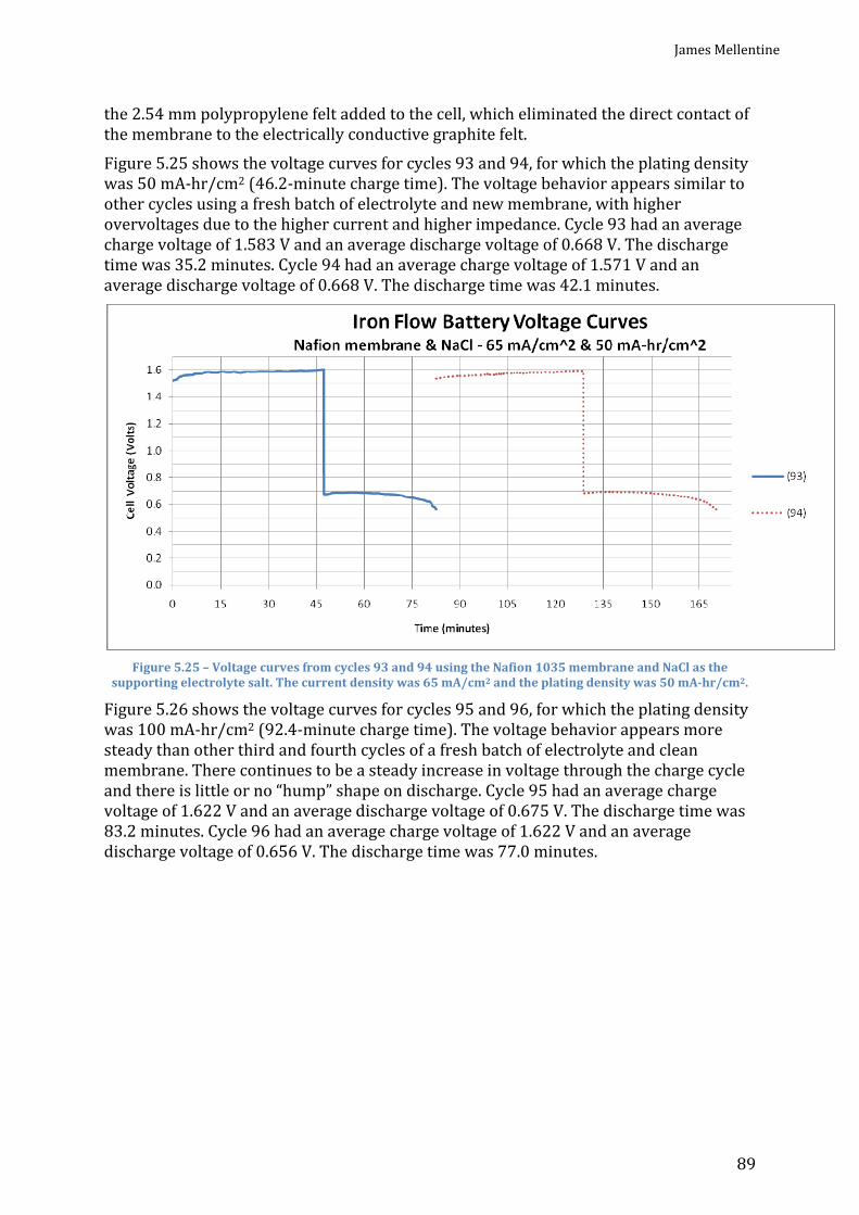
James Mellentine
89
the 2.54 mm polypropylene felt added to the cell, which eliminated the direct contact of the membrane to the electrically conductive graphite felt. Figure 5.25 shows the voltage curves for cycles 93 and 94, for which the plating density was 50 mA-hr/cm2 (46.2-minute charge time). The voltage behavior appears similar to other cycles using a fresh batch of electrolyte and new membrane, with higher overvoltages due to the higher current and higher impedance. Cycle 93 had an average charge voltage of 1.583 V and an average discharge voltage of 0.668 V. The discharge time was 35.2 minutes. Cycle 94 had an average charge voltage of 1.571 V and an average discharge voltage of 0.668 V. The discharge time was 42.1 minutes.
Figure 5.25 – Voltage curves from cycles 93 and 94 using the Nafion 1035 membrane and NaCl as the
supporting electrolyte salt. The current density was 65 mA/cm2 and the plating density was 50 mA-hr/cm2. Figure 5.26 shows the voltage curves for cycles 95 and 96, for which the plating density was 100 mA-hr/cm2 (92.4-minute charge time). The voltage behavior appears more steady than other third and fourth cycles of a fresh batch of electrolyte and clean membrane. There continues to be a steady increase in voltage through the charge cycle and there is little or no “hump” shape on discharge. Cycle 95 had an average charge voltage of 1.622 V and an average discharge voltage of 0.675 V. The discharge time was 83.2 minutes. Cycle 96 had an average charge voltage of 1.622 V and an average discharge voltage of 0.656 V. The discharge time was 77.0 minutes.

Chapter 5: Laboratory Performance of an Iron Hybrid Flow Battery
90
Figure 5.26 – Voltage curves from cycles 95 and 96 using the Nafion 1035 membrane and NaCl as the
supporting electrolyte salt. The current density was 65 mA/cm2 and the plating density was 100 mA-hr/cm2. The voltaic, coulombic, and energy efficiency values were calculated for these cycles and are shown in Figure 5.27. At a quick glance, all efficiency values are much more consistent over the four cycles than with previous sets of data. This may be due to avoidance of buildup on the membrane by adding the PP felt to the negative side of the cell. However, the absolute performance is not better. The voltaic efficiency, though steady, stayed in a relatively low range between 40.4% and 42.5%. Coulombic efficiency was also steadier, and showed relatively good performance, ranging between 74.3% and 91.2%. The energy efficiencies were steady but relatively poor, ranging between 31.3% and 38.8%.
Figure 5.27 – The efficiencies calculated from this set of data are much more consistent over 4 consecutive
cycles than with other cycles, even if the overall performance is lower. This may be due to avoidance of buildup on the membrane with the addition of an inert (PP) felt material in the cell.

James Mellentine
91
The next cycle (97) was intended to run at a current density of 80 mA/cm2, with a plating density of 50 mA-hr/cm2 (37.5-minute charge time). Shown in Figure 5.28, the voltage was steady during charge, but the overvoltage is quite large. The average charge voltage was 1.908 V. When the discharge was attempted, the load was not able to maintain a steady current, indicating that the voltage was very low. Therefore, the battery was discharged at a current density of 50 mA/cm2, with an average discharge voltage of 0.683 V. The discharge time was 52.7 minutes. The voltaic efficiency for the cycle was 35.8%, while the coulombic efficiency was 85.6%. The overall energy efficiency was 30.7%, only slightly lower than the previous four cycles above.
Figure 5.28 – Voltage curve from cycle 97 using the Nafion 1035 membrane and NaCl as the supporting
electrolyte salt. The current density was 80 mA/cm2 on charge and 50 mA/cm2 on discharge. The plating density was 50 mA-hr/cm2. The follow-up and final cycle 98, shown in Figure 5.29, was intended to be another test with a current density of 50 mA/cm2 and plating density of 100 mA-hr/cm2, since only one good cycle in this scenario was conducted previously. Again, the voltage was steady, but the overvoltage was large – larger even than the earlier tests at 65 mA/cm2, indicating deterioration in cell performance. The average charge voltage was 1.728 V. Similar to the previous cycle, the load was not able to maintain a steady current on discharge, indicating that the voltage was very low and providing evidence of further performance deterioration. Therefore, the battery was discharged at a current density of 20 mA/cm2, with an average discharge voltage of 0.866 V. The discharge time was 259.5 minutes. The voltaic efficiency for the cycle was 50.1%, while the coulombic efficiency was 86.5%. The overall energy efficiency was 43.3%, slightly higher than previous cycles using this batch of electrolyte. After this final cycle, the cell was disassembled. The PP felt layer appeared to have significantly decreased the amount of matter that was deposited onto the membrane. Only a very small area in the upper corner near the electrolyte exit point was there the appearance of a solid layer deposited onto the membrane. This area also corresponded to the darkest discoloration on the PP felt. The PP felt is normally white in color, and about a third of the PP felt had turned a dark gray color, possibly indicating the strongest points of iron plating. The discolored area was also closest to the electrolyte
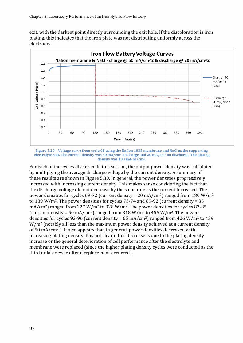
Chapter 5: Laboratory Performance of an Iron Hybrid Flow Battery
92
exit, with the darkest point directly surrounding the exit hole. If the discoloration is iron plating, this indicates that the iron plate was not distributing uniformly across the electrode.
Figure 5.29 – Voltage curve from cycle 98 using the Nafion 1035 membrane and NaCl as the supporting
electrolyte salt. The current density was 50 mA/cm2 on charge and 20 mA/cm2 on discharge. The plating density was 100 mA-hr/cm2. For each of the cycles discussed in this section, the output power density was calculated by multiplying the average discharge voltage by the current density. A summary of these results are shown in Figure 5.30. In general, the power densities progressively increased with increasing current density. This makes sense considering the fact that the discharge voltage did not decrease by the same rate as the current increased. The power densities for cycles 69-72 (current density = 20 mA/cm2) ranged from 180 W/m2 to 189 W/m2. The power densities for cycles 73-74 and 89-92 (current density = 35 mA/cm2) ranged from 227 W/m2 to 328 W/m2. The power densities for cycles 82-85 (current density = 50 mA/cm2) ranged from 318 W/m2 to 456 W/m2. The power densities for cycles 93-96 (current density = 65 mA/cm2) ranged from 426 W/m2 to 439 W/m2 (notably all less than the maximum power density achieved at a current density of 50 mA/cm2.) It also appears that, in general, power densities decreased with increasing plating density. It is not clear if this decrease is due to the plating density increase or the general deterioration of cell performance after the electrolyte and membrane were replaced (since the higher plating density cycles were conducted as the third or later cycle after a replacement occurred).

James Mellentine
93
Figure 5.30 – Calculated power densities for charge and discharge cycles for varying current densities
discussed in this chapter. The output specific energy (by mass of plated iron) was calculated by multiplying the average power by the discharge time and dividing by the total mass of plated iron. The mass of plated iron was calculated by multiplying the plating density, cell area, and molar weight of iron and dividing by the Faraday constant. A summary of these results are shown in Figure 5.31.
Figure 5.31 – Calculated energy densities based on volume and mass for charge and discharge cycles for
varying current densities discussed in this chapter. Specific energies varied widely between 247 Wh/kg and 770 Wh/kg. Lower energies were calculated for higher plating densities except for the highest current density tested, which had higher specific energies for the higher plating density cycles.

Chapter 5: Laboratory Performance of an Iron Hybrid Flow Battery
94
A summary of measurements and performance calculations for the cycles discussed in this section are shown in Table 5.5. These same data points are available in Appendix B for the cycles not presented in this section. Table 5.5 – A summary of measured data and calculated performance values for the cycles discussed in this section.
Cycle # Charge/discharge current density (mA/cm2) Charge/discharge time (min) Avg. charge/discharge voltage (V) Voltaic/Coulombic/Energy efficiency (%) Power density (W/m2) Energy delivered (Wh) Specific energy (Wh/kg)69 20/20 150/64.6 1.238/0.946 76.4%/43%/32.9% 189 1.018 391 70 20/20 150/126.6 1.257/0.946 75.3%/84.3%/63.5% 189 1.996 766 71 20/20 184/159.2 1.349/0.927 68.7%/86.5%/59.4% 185 2.459 770 72 20/20 300/212.1 1.358/0.902 66.4%/70.7%/47% 180 3.189 612 73 35/35 85.8/47.6 1.42/0.745 52.5%/55.4%/29.1% 261 1.034 397 74 35/35 85.8/44.2 1.403/0.648 46.1%/51.5%/23.8% 227 0.834 320 82 50/50 60/41.8 1.336/0.912 68.2%/69.6%/47.5% 456 1.587 609 83 50/50 60/53.4 1.403/0.855 60.9%/88.9%/54.1% 427 1.900 729 84 50/50 120/65.2 1.451/0.696 48%/54.3%/26.1% 348 1.892 363 85 50/50 2/1.9 1.533/0.636 41.5%/95.7%/39.7% 318 0.049 584 89 35/35 85.8/65.2 1.26/0.937 74.3%/76%/56.5% 328 1.781 684 90 35/35 85.8/71.2 1.35/0.915 67.8%/83%/56.3% 320 1.900 729 91 35/35 171.5/81.1 1.344/0.806 60%/47.3%/28.4% 282 1.906 366 92 35/35 171.5/57.1 1.32/0.774 58.7%/33.3%/19.5% 271 1.289 247 93 65/65 47.3/35.2 1.583/0.668 42.2%/74.3%/31.3% 434 1.272 476 94 65/65 46.2/42.1 1.571/0.668 42.5%/91.2%/38.8% 434 1.525 585 95 65/65 94.1/83.2 1.622/0.675 41.6%/88.4%/36.8% 439 3.043 573 96 65/65 92.4/77 1.622/0.656 40.4%/83.4%/33.7% 426 2.735 525 97 80/50 38.5/52.7 1.908/0.683 35.8%/85.6%/30.7% 342 1.502 562 98 50/20 120/259.5 1.728/0.866 50.1%/86.5%/43.3% 173 3.744 719 In summary, this table represents data from 20 complete charge & discharge cycles of an iron hybrid flow battery. Current densities ranged from 20 mA/cm2 to 80 mA/cm2, while plating densities ranged from 50 mA-hr/cm2 to 100 mA-hr/cm2. In general, the performance was the best within two cycles immediately following a change in electrolyte and membrane. The polypropylene felt helped to make the performance
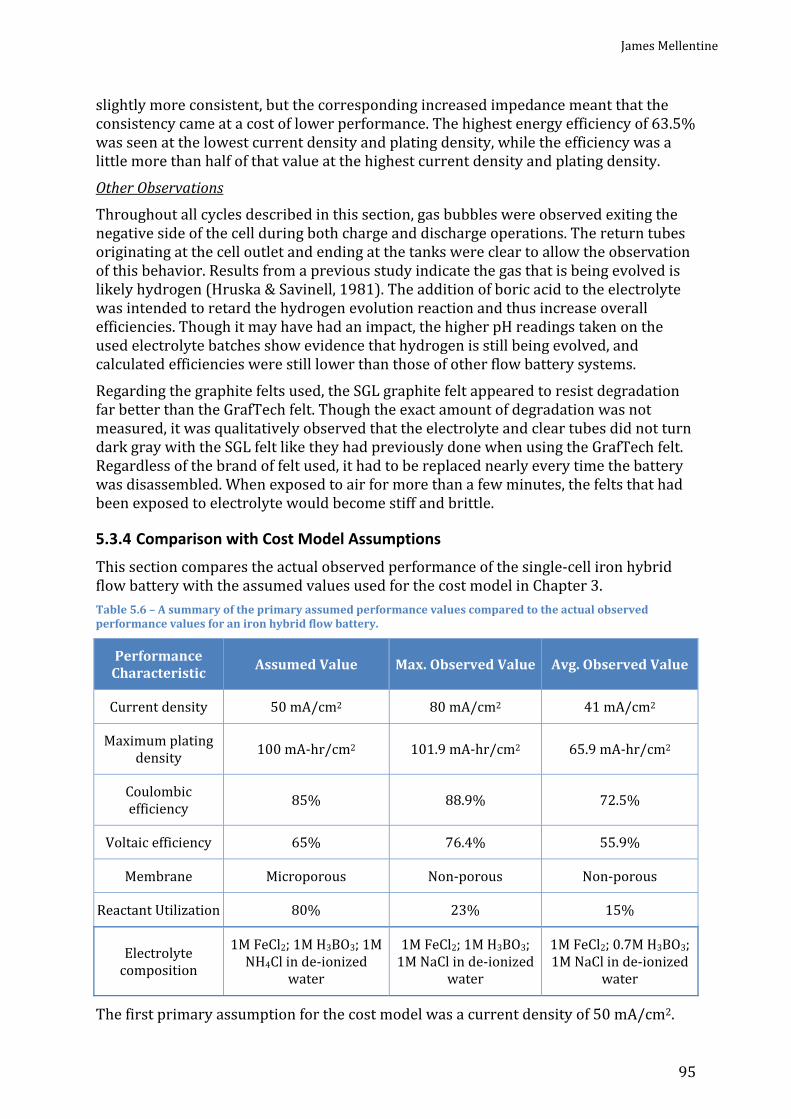
James Mellentine
95
slightly more consistent, but the corresponding increased impedance meant that the consistency came at a cost of lower performance. The highest energy efficiency of 63.5% was seen at the lowest current density and plating density, while the efficiency was a little more than half of that value at the highest current density and plating density. Other Observations Throughout all cycles described in this section, gas bubbles were observed exiting the negative side of the cell during both charge and discharge operations. The return tubes originating at the cell outlet and ending at the tanks were clear to allow the observation of this behavior. Results from a previous study indicate the gas that is being evolved is likely hydrogen (Hruska & Savinell, 1981). The addition of boric acid to the electrolyte was intended to retard the hydrogen evolution reaction and thus increase overall efficiencies. Though it may have had an impact, the higher pH readings taken on the used electrolyte batches show evidence that hydrogen is still being evolved, and calculated efficiencies were still lower than those of other flow battery systems. Regarding the graphite felts used, the SGL graphite felt appeared to resist degradation far better than the GrafTech felt. Though the exact amount of degradation was not measured, it was qualitatively observed that the electrolyte and clear tubes did not turn dark gray with the SGL felt like they had previously done when using the GrafTech felt. Regardless of the brand of felt used, it had to be replaced nearly every time the battery was disassembled. When exposed to air for more than a few minutes, the felts that had been exposed to electrolyte would become stiff and brittle. 5.3.4 Comparison with Cost Model Assumptions This section compares the actual observed performance of the single-cell iron hybrid flow battery with the assumed values used for the cost model in Chapter 3. Table 5.6 – A summary of the primary assumed performance values compared to the actual observed performance values for an iron hybrid flow battery.
Performance Characteristic Assumed Value Max. Observed Value Avg. Observed Value
Current density 50 mA/cm2 80 mA/cm2 41 mA/cm2 Maximum plating density 100 mA-hr/cm2 101.9 mA-hr/cm2 65.9 mA-hr/cm2 Coulombic efficiency 85% 88.9% 72.5%
Voltaic efficiency 65% 76.4% 55.9% Membrane Microporous Non-porous Non-porous Reactant Utilization 80% 23% 15% Electrolyte composition 1M FeCl2; 1M H3BO3; 1M NH4Cl in de-ionized water 1M FeCl2; 1M H3BO3; 1M NaCl in de-ionized water 1M FeCl2; 0.7M H3BO3; 1M NaCl in de-ionized water The first primary assumption for the cost model was a current density of 50 mA/cm2.

Chapter 5: Laboratory Performance of an Iron Hybrid Flow Battery
96
The observations made in this study show that an iron hybrid flow battery can operate at that current density. While the maximum attempted value of 80 mA/cm2 was able to charge successfully, it could not discharge at that level, and so the practical maximum charge density of this cell was 65 mA/cm2. Also, the best efficiencies were achieved at lower current densities. The average current density of the 20 cycles presented in the previous section was 41 mA/cm2. Overall, the assumed current density of 50 mA/cm2 is a reasonable assumption. The next assumption for the cost model was a maximum plating density of 100 mA-hr/cm2. The observations made in this study show that an iron hybrid flow battery can operate at that plating density, with the maximum attempted value being 101.9 mA-hr/cm2. The average plating density of the 20 cycles presented in the previous section was 65.9 mA/cm2. In some of the experiments using microporous separators (discussed in Appendix B) steady voltage behavior was shown up to about 167 mA-hr/cm2. Overall, the assumed current density of 100 mA-hr/cm2 appears to be a reasonable assumption. The assumed coulombic efficiency was 85%. The maximum observed value (not counting the two-minute cycle 85) was 88.9%, which shows that this level of performance can be achieved. The average observed value of 72.5% shows that this level was not consistently achieved. Overall, the assumed coulombic efficiency is reasonable, but further research and development is necessary to achieve that on a consistent basis. A similar assessment can be made for the voltaic efficiency assumption of 65%. The maximum observed value was 76.4% while the average value of 55.9% shows that it was not achieved consistently. Overall, the assumed voltaic efficiency is reasonable, but further research and development is necessary to achieve it on a consistent basis. The assumed membrane for the commercial system was a Daramic microporous membrane. This membrane was used in a previous study with no crossover problems indicated, and was used to successfully measure useful symmetric cell results in this study (Hruska & Savinell, 1981). This problem (likely a mechanical design or pressure difference issue) could have been further investigated and likely resolved with some slight design changes to the flow block and cell pieces and/or the addition of a more sophisticated pressure regulation system on each side of the cell. However, time constraints of the study forced a more immediate solution of using a non-porous membrane for the remainder of the data collection period. So, even though very little data was obtained using the assumed material, the author argues that it is still a reasonable assumption in a commercial system. The design system was assumed to have a state of charge range of 10%-90%. Based on the symmetric cell observations, it was shown that the positive electrolyte exhibited consistently steady voltage behavior only within a reaction usage percent of about 67%. This would similarly limit the operations of the iron hybrid flow cell, so operating above that level is not immediately practical with the given chemistry. In addition, the experiments used only about 23% of the maximum theoretical plating capacity of the cell, much less than the 90% that would be required in the design. Therefore the assumed SOC range is likely not a reasonable assumption and further research and development would need to occur to achieve this target. However, the immediate remedy to this is simply to have a larger volume of electrolyte in each system. Given the very low cost of electrolyte compared to the overall system (3%), this would not significantly increase the cost of the system.

James Mellentine
97
The final major assumption for the cost model was the chemistry of the electrolyte. The model assumes 1 M each of ferrous chloride, boric acid, and ammonium chloride. The 1 M FeCl2 was clearly reasonable, since all 20 cycles used this concentration. The 1 M NH4Cl was substituted with NaCl in the performance tests due to its incompatibility with Nafion. However, the NH4Cl is compatible with the proposed microporous membrane, and given the results from the symmetric cell tests with that chemistry, it is a reasonable assumption. The 1 M H3BO3 was used for some of the tests and was only decreased due to deformation of the PVC pieces in the cell. Since the proposed operating temperature of the commercial cell is lower and deformation is likely not as much of a concern, the 1 M boric acid is reasonable since it is still soluble at the proposed operating temperature of 40 ˚C. The problem is not with the electrolyte, it is with the crossover behavior in the microporous membrane as described above. Overall, the assumed electrolyte concentration is a reasonable assumption. In summary, all of the assumed values were used/achieved during some portion of the tests, and even though some further work is necessary to improve consistency of results (and resolve the crossover problem), all of the assumed values appear to be reasonable for a mass-produced commercial system.

Chapter 5: Laboratory Performance of an Iron Hybrid Flow Battery
98

James Mellentine
99
Chapter 6: Conclusions This chapter summarizes the findings of this study. Included are key findings regarding the design and cost of the proposed system, the performance of the system in an area regulation application, and the data collected during laboratory experiments. 6.1 Design and Cost of an Iron Hybrid Flow Battery A modular iron hybrid flow battery system was designed with a power capacity 10 kW and an energy capacity of 20.9 kWh, with an assumed coulombic efficiency of 85% and voltaic efficiency of 65%. The calculated power density of the battery is 48 mW/cm2. With 78 cells in the stack, it has a stack voltage of 75.5 V. To achieve the maximum plating density of 100 mA-hr/cm2 while staying in a state of charge range of 10% - 90%, the battery requires a total electrolyte volume of 1638 L (1092 L on the positive side and 546 L on the negative side). This equates to an energy density of 12.7 Wh/L. The maximum pump flow rate required is 109.1 L/min. The average internal pressure of the system is under 2 bar, which equates to an average parasitic pumping loss of 1.25%. At full charge, the battery can provide 2 hours of discharge time. A summary of assumed and calculated design parameters are listed in Table 6.1. Table 6.1 – Summary of assumed and calculated design parameters for the 10 kW modular iron hybrid flow battery.
Parameter Value Parameter Value Modular power capacity 10 kW Parasitic & inverter losses 12% Annual production 1000 units Membrane MicroporousCell area 3000 cm2 Number of cells 78 Nominal cell voltage 1.2 V Stack voltage 75.5 V Electrolyte composition 1M FeCl2; 1M H3BO3; 1M NH4Cl in deionized water Energy capacity 20.9 kWh SOC range 10% - 90% Max. pump flow rate 109 L/min Current density 50 mA/cm2 Avg. internal pressure 1.76 bar Max. plating density 100 mA-hr/cm2 Total electrolyte volume 1637 L Energy efficiency 55% Discharge time @ 90% SOC 125 minutesAssuming an annual production of 1000 of these modular units, the required annual supply of each battery component was determined. In collaboration with InnoVentures, a cost estimate was determined for the graphite felt, bipolar plates, flow frames, gaskets, collector plates, end plates, bolts, PVC plumbing, pumps, and a control system. Daramic provided cost estimates for the membrane separator. Brenntag provided cost estimates for boric acid, ammonium chloride, and de-ionized water. PVS Chemicals provided the cost estimate for ferrous chloride solution. An estimate for tank prices was obtained by a distributor of Den Hartog Industries. Table 6.2 shows annual quantities and cost estimates for each component.

Chapter 6: Conclusions
100
Table 6.2 – Summary of components of an iron hybrid flow battery system, along with annual required quantities and estimated unit costs assuming 1000 units of annual production.
Component Annual qty. Optimistic cost Most likely cost Pessimistic costActivated felt 46,800 m2 $80.00/m2 $90.00/m2 $100.00/m2 Bipolar plates 79,000 $35.00 each $50.00 each $55.00 each Flow frames 79,000 $25.00 each $32.00 each $60.00 each Gaskets 154,000 $1.00 each $2.00 each $2.50 each Collector plates 2,000 $96.63 each $125.00 each $150.00 each End plates 2,000 $86.28 each $175.00 each $192.50 each Bolts 12,000 $10.00 each $12.50 each $15.00 each PVC 1,000 $100.00/set $150.00/set $200.00/set Daramic separator 25,104 m2 $3.50/m2 $4.35/m2 $80.00/m2 Ferrous chloride solution (27%) 581,386 L $0.079/L $0.129/L $0.180/L Ammonium chloride 87,617 kg $0.86/kg $1.06/kg $1.12/kg Boric acid 101,278 kg $1.63/kg $1.96/kg $2.09/kg De-ionized water 925,574 L $0.016/L $0.016/L $0.238/L Electrolyte preparation 100 batches $50.00/batch $100.00/batch $150.00/batch Tanks 1,000 pairs $276.97/pair $276.97/pair $318.05/pair Pumps 2,000 $100.00 each $200.00 each $300.00 each Control system 1,000 $100.00 each $600.00 each $800.00 each Three Point Estimation was used to determine an expected system cost of $14,924. This is $1492/kW and $715/kWh. A large majority (77%) of the system cost was from the graphite felt, bipolar plates, and flow frame assemblies. In contrast to studies of vanadium systems in which the electrolyte can be as much as 80% of system cost, the electrolyte cost for the iron hybrid flow battery was only 3% of the total system cost. Not surprisingly, the total system cost per kW and per kWh was most sensitive to the most expensive components – graphite felt, bipolar plates, and flow frames. To most effectively bring down the cost of this battery, efforts should focus on decreasing the unit cost of these three components. In regards to technical performance, the cost per kW was found to be most sensitive to current density, followed secondarily to voltaic efficiency. Increasing the current density and increasing voltaic efficiency can bring down the cost of the battery per kW because less/smaller cell sizes would be needed. The cost per kWh was found to be most sensitive to plating density, and secondarily on coulombic and voltaic efficiency. Increasing the maximum plating density would allow more energy to be stored per volume of electrolyte and proportionally increase the energy capacity of the battery. Likewise, reducing efficiency losses would also increase the energy capacity of the battery. On the contrary, an increased current density would effectively increase the cost per kWh. This factor then must be balanced with its tendency to decrease cost per kW. To most effectively decrease the cost of this battery by performance improvements, research efforts should focus on finding an optimal

James Mellentine
101
current density and improving voltaic efficiency, with a secondary focus on improving coulombic efficiency. On a cost per kW basis, the iron hybrid flow battery outperforms published costs for both vanadium systems and zinc bromine systems. On a cost per kWh basis, the iron hybrid flow battery slightly beat published costs of the zinc bromide battery. However, due to the extremely large energy capacities of vanadium systems, their published costs per kW were lower than the iron system. One of the clear cost advantages for the iron hybrid flow battery is the low cost of electrolyte. The cost of vanadium for the vanadium electrolyte was calculated to be $3.22/L, assuming a 2 M vanadium solution – and this does not include the other electrolyte components such as water and sulfuric acid. The complete cost of the electrolyte in the proposed iron hybrid flow battery is only $0.233/L, or 7% of the minimum cost for the vanadium-based electrolyte. 6.2 Simulation of a Large Iron Hybrid Flow Battery System The performance of the iron hybrid flow battery was analyzed in a hypothetical application, with a scaled-up 2 MW system providing area regulation services. This application was selected from a list of energy storage grid applications detailed by a previous study. Many of the applications were excluded due to the long discharge time requirements. Of the remaining applications, the area regulation application appeared to have the largest monetary benefit. Using published data from the California Independent Service Operator (CAISO) and making some operational assumptions, several performance results were calculated. During the year of simulated operation, the battery cycled 714 times, or about 2 cycles per day, with an average state of charge of 41.4%. The total electricity purchased during charge operations was 6159 MWh, and the total electricity sold during discharge operations was 2625 MWh. The battery was available for up regulation 56.7% of the time and available for down regulation 96.9% of the time. Using the regulation revenue data and market price of electricity, the battery was projected to have a net loss in this application, with increased energy efficiency necessary to decrease the cost differential between purchased & sold electricity. A summary of assumed and calculated parameters for this simulation are listed in Table 6.3. Table 6.3 – Summary of assumed and calculated simulation parameters for a 2 MW iron hybrid flow battery system performing an area regulation application.
Parameter Value Parameter Value Power capacity 2 MW Average SOC 41.4% Energy efficiency 55% # cycles per year 714 Parasitic & inverter losses 12% Up regulation availability 56.7% SOC range 10% - 90% Down regulation availability 96.9% Charge/discharge time 30 minutes per hour Total electricity purchased 6159 MWh Electricity price $163.3/MWh Total electricity sold 2625 MWh Inflation rate 2.5% Net revenue -$98,586 In order for the battery to break-even (area regulation revenue plus electricity sales revenue minus electricity costs), an energy efficiency of 64% would be needed. A

Chapter 6: Conclusions
102
revenue-positive scenario of over $100,000/year was calculated for an energy efficiency of 75% - this could serve as an initial target for future research and development efforts. 6.3 Actual Performance of a Small Iron Hybrid Flow Battery A 50 cm2 cell was used to cycle the iron-based electrolyte for varying current densities and plating densities. Several electrolyte batches were prepared throughout the cycles. Symmetric cell tests were first conducted that had a mixture of ferric and ferrous ions to mimic the positive side chemistry. To avoid crossover problems, the membrane was switched to Nafion, while the supporting electrolyte was switched to sodium chloride due to ammonium chloride’s incompatibility with Nafion. During regular tests, the electrolyte contained 1 M ferrous chloride, 1 M sodium chloride, and 0.7 M boric acid, with an operating temperature of 45 ˚C. The average starting pH of the electrolyte solution was 2.03. A symmetric electrolyte was first studied in the cell to confirm the stability of the positive-side reactions. Using a microporous membrane, the cell was cycled six times each at current densities of 50 mA/cm2 and 100 mA/cm2. At the lower current, the overvoltage was seen to be low and consistent, rising from 0.03 V to about 0.2 V in 150 minutes of charge time. At the higher current, the overvoltage was seen to also be low and consistent, starting at 0.13 V and rising to about 0.3 V in 75 minutes. After moving to the Nafion membrane and new electrolyte, similar tests were conducted over a broader range of currents. Each case showed very consistent and repeatable voltage behavior, with gradually increasing overvoltage with increasing current density. These tests showed the positive side electrolyte has a reactant utilization limit of about 67%. Moving on to the iron hybrid flow cell tests, the cell was cycled at current densities of 20 mA/cm2, 35 mA/cm2, 50 mA/cm2, and 65 mA/cm2, each at plating densities of 50 mA-hr/cm2 and 100 mA-hr/cm2. In general, performance of the battery quickly deteriorated after only 2-3 cycles of freshly prepared electrolyte and fresh membrane and electrodes. Based on observations of the cell and membrane during several disassemblies, one component of this deterioration strongly points to iron plating onto the negative side of the membrane and slowing/blocking the electrochemical reactions. Performance deterioration could also partly be due to hydrogen evolution and pH changes in the electrolyte. Further detailed experiments are required to confirm the exact modes of deteriorating performance. At 20 mA/cm2, the voltaic efficiency declined through the first 4 cycles from 76.4% to 66.4%, while the coulombic efficiencies initial increased from 43% to 86.5% and then declining again. Energy efficiencies ranged from 32.9% to 63.5%. At 35 mA/cm2, the voltaic efficiency again declined through 4 cycles from 74.3% to 58.7%. The coulombic efficiencies were 76% and 83% at the lower plating density, and then significantly decreased to 47.3% and 33.3% for the higher plating density. Energy efficiencies ranged from 19.5% to 56.5%. At 50 mA/cm2, the voltaic efficiency similarly declined through 3 cycles from 68.2% to 48%. The coulombic efficiencies were higher for the lower plating density (66.9% - 88.9%) and then significantly decreased with the higher plating density (54.2%). Energy efficiencies ranged from 26.1% to 54.1%. Before the final set of tests, an inert (PP) felt spacer was added next to the membrane on the negative side of the cell to help prevent plating on the membrane. This seemed to
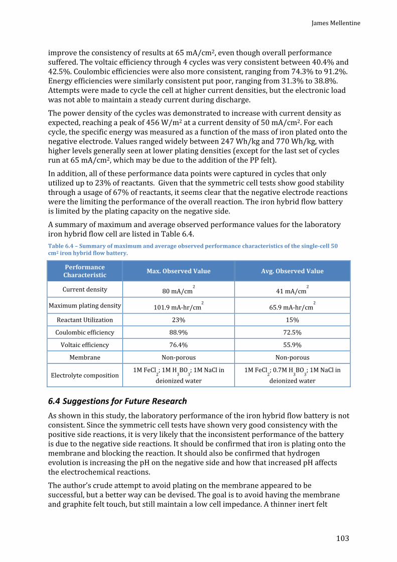
James Mellentine
103
improve the consistency of results at 65 mA/cm2, even though overall performance suffered. The voltaic efficiency through 4 cycles was very consistent between 40.4% and 42.5%. Coulombic efficiencies were also more consistent, ranging from 74.3% to 91.2%. Energy efficiencies were similarly consistent put poor, ranging from 31.3% to 38.8%. Attempts were made to cycle the cell at higher current densities, but the electronic load was not able to maintain a steady current during discharge. The power density of the cycles was demonstrated to increase with current density as expected, reaching a peak of 456 W/m2 at a current density of 50 mA/cm2. For each cycle, the specific energy was measured as a function of the mass of iron plated onto the negative electrode. Values ranged widely between 247 Wh/kg and 770 Wh/kg, with higher levels generally seen at lower plating densities (except for the last set of cycles run at 65 mA/cm2, which may be due to the addition of the PP felt). In addition, all of these performance data points were captured in cycles that only utilized up to 23% of reactants. Given that the symmetric cell tests show good stability through a usage of 67% of reactants, it seems clear that the negative electrode reactions were the limiting the performance of the overall reaction. The iron hybrid flow battery is limited by the plating capacity on the negative side. A summary of maximum and average observed performance values for the laboratory iron hybrid flow cell are listed in Table 6.4. Table 6.4 – Summary of maximum and average observed performance characteristics of the single-cell 50 cm2 iron hybrid flow battery.
Performance Characteristic Max. Observed Value Avg. Observed Value Current density 80 mA/cm2 41 mA/cm2 Maximum plating density 101.9 mA-hr/cm2 65.9 mA-hr/cm2 Reactant Utilization 23% 15% Coulombic efficiency 88.9% 72.5% Voltaic efficiency 76.4% 55.9% Membrane Non-porous Non-porous Electrolyte composition 1M FeCl2; 1M H3BO3; 1M NaCl in deionized water 1M FeCl2; 0.7M H3BO3; 1M NaCl in deionized water
6.4 Suggestions for Future Research As shown in this study, the laboratory performance of the iron hybrid flow battery is not consistent. Since the symmetric cell tests have shown very good consistency with the positive side reactions, it is very likely that the inconsistent performance of the battery is due to the negative side reactions. It should be confirmed that iron is plating onto the membrane and blocking the reaction. It should also be confirmed that hydrogen evolution is increasing the pH on the negative side and how that increased pH affects the electrochemical reactions. The author’s crude attempt to avoid plating on the membrane appeared to be successful, but a better way can be devised. The goal is to avoid having the membrane and graphite felt touch, but still maintain a low cell impedance. A thinner inert felt
Chapter 6: Conclusions
104
material or inert porous material could be used for this purpose. Or a spacer could be eliminated altogether if a structure cage were built into the PVC spacer – 2-3 thin horizontal and vertical strips could likely keep the felt compressed against the graphite plate with space maintained between the felt and membrane. More detailed research should also be pursued regarding the plating and stripping reactions of iron. To make observations easier, this could be done outside of a battery cell, perhaps on a rotating disk electrode. The overpotentials of the plating and stripping reactions could be measured, along with the conditions that seem to reduce the evolution of hydrogen. Perhaps a different electrode material besides graphite is a better substrate on which to plate the iron. A more consistent plating and stripping reaction will be a key factor to improving the consistency of the iron hybrid flow battery. The elimination of electrolyte crossover between negative and positive sides would significantly increase the consistency of performance with microporous membranes. Crossover could be reduced with an improved cell design that promotes more uniform flow and decreased pressure drops. A pressure gauge could be installed on each side of the cell to determine if there is a pressure difference, as a way to evaluate cell designs. A digital pressure gauge could be integrated into the control system. If two pumps were used (one for each side of the cell), a difference in pressure could signal the control system to automatically increase the pump speed on one side within preset limits, or automatically shut down if the pressure differences become too much for the system to compensate. Besides improving consistency, research should be conducted to improve the performance of the battery in general. Performance appears to decrease with increasing plating density. Increasing the performance of the battery at a plating density of 100 mA-hr/cm2 could help move a commercial product closer to reality. And moving beyond this level to 150 or 200 mA-hr/cm2 would significantly increase energy density and reduce cost per kWh. This effort would have to focus on the reactions on both sides of the cell. The symmetric cell tests in this study showed the positive electrolyte performs well only up to a reactant utilization of 67%. Increasing this will likely require changes to the electrolyte. Research should try different supporting electrolytes or new positive-side ligands. The negative side will require well-formed plate structures on the electrode, without internal stress fractures or dendrite formations. Experiments with new supporting electrolytes and ligands should be conducted to improve the plating quality needed to support a thicker plate. These chemistry changes should also study how it affects hydrogen evolution. An ideal additive will allow high reactant utilization, a high-quality plate, and reduce the amount of hydrogen evolved. The development of a model would also be helpful for understanding the effects of varying current density, plating density, and electrolyte concentrations. Similar to the models developed for other battery technologies mentioned in Chapter 2, a model based on conservation of mass, energy, charge, and momentum, along with kinetic models of iron-based reactions from the Butler-Volmer equation and other relevant concepts. This model should be validated with experimental results. A model like this could save valuable time by showing the effects of varying pump flow rates, current density, plating density, temperature changes, and electrolyte concentrations on battery performance without all the necessary laboratory experiments. This could help target more valuable

James Mellentine
105
and potentially promising electrolyte and cell configurations to test in the laboratory, and thus increase the speed of incremental improvements. Finally, the iron hybrid flow battery was shown to not be financially viable in an area regulation application, assuming 55% efficiency. Further simulation and economic analysis of the battery in other applications should be conducted. A more detailed analysis of what performance conditions or capital cost would make the battery profitable are needed to further refine development targets and define potential market opportunities for the technology.

106
Appendix A The cost model spreadsheet used to calculate the results discussed in Chapter 3 is included within the following link: Cost Model_Iron
Flow Battery_FINAL.x In addition, screenshots of the spreadsheet with formulas shown follows:

James Mellentine
107

108

James Mellentine
109
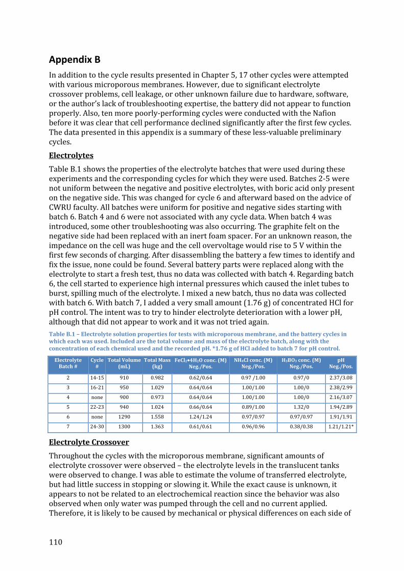
110
Appendix B In addition to the cycle results presented in Chapter 5, 17 other cycles were attempted with various microporous membranes. However, due to significant electrolyte crossover problems, cell leakage, or other unknown failure due to hardware, software, or the author’s lack of troubleshooting expertise, the battery did not appear to function properly. Also, ten more poorly-performing cycles were conducted with the Nafion before it was clear that cell performance declined significantly after the first few cycles. The data presented in this appendix is a summary of these less-valuable preliminary cycles. Electrolytes Table B.1 shows the properties of the electrolyte batches that were used during these experiments and the corresponding cycles for which they were used. Batches 2-5 were not uniform between the negative and positive electrolytes, with boric acid only present on the negative side. This was changed for cycle 6 and afterward based on the advice of CWRU faculty. All batches were uniform for positive and negative sides starting with batch 6. Batch 4 and 6 were not associated with any cycle data. When batch 4 was introduced, some other troubleshooting was also occurring. The graphite felt on the negative side had been replaced with an inert foam spacer. For an unknown reason, the impedance on the cell was huge and the cell overvoltage would rise to 5 V within the first few seconds of charging. After disassembling the battery a few times to identify and fix the issue, none could be found. Several battery parts were replaced along with the electrolyte to start a fresh test, thus no data was collected with batch 4. Regarding batch 6, the cell started to experience high internal pressures which caused the inlet tubes to burst, spilling much of the electrolyte. I mixed a new batch, thus no data was collected with batch 6. With batch 7, I added a very small amount (1.76 g) of concentrated HCl for pH control. The intent was to try to hinder electrolyte deterioration with a lower pH, although that did not appear to work and it was not tried again. Table B.1 – Electrolyte solution properties for tests with microporous membrane, and the battery cycles in which each was used. Included are the total volume and mass of the electrolyte batch, along with the concentration of each chemical used and the recorded pH. *1.76 g of HCl added to batch 7 for pH control.
Electrolyte Batch #
Cycle #
Total Volume (mL)
Total Mass(kg)
FeCl2•4H2O conc. (M) Neg./Pos.
NH4Cl conc. (M) Neg./Pos.
H3BO3 conc. (M) Neg./Pos.
pHNeg./Pos. 2 14-15 910 0.982 0.62/0.64 0.97 /1.00 0.97/0 2.37/3.083 16-21 950 1.029 0.64/0.64 1.00/1.00 1.00/0 2.38/2.994 none 900 0.973 0.64/0.64 1.00/1.00 1.00/0 2.16/3.075 22-23 940 1.024 0.66/0.64 0.89/1.00 1.32/0 1.94/2.896 none 1290 1.558 1.24/1.24 0.97/0.97 0.97/0.97 1.91/1.917 24-30 1300 1.363 0.61/0.61 0.96/0.96 0.38/0.38 1.21/1.21*
Electrolyte Crossover Throughout the cycles with the microporous membrane, significant amounts of electrolyte crossover were observed – the electrolyte levels in the translucent tanks were observed to change. I was able to estimate the volume of transferred electrolyte, but had little success in stopping or slowing it. While the exact cause is unknown, it appears to not be related to an electrochemical reaction since the behavior was also observed when only water was pumped through the cell and no current applied. Therefore, it is likely to be caused by mechanical or physical differences on each side of

111
the cell – perhaps pressure differences due to slightly different hose lengths or perhaps the flow on one side is slightly more turbulent than the other due to differences in felt or the fit of the cell layers. It is also possible that there are small punctures in the membrane itself that may not be observable with the naked eye. Figure B.1 shows the estimated crossover rates throughout these cycles. These were estimated based on observations of how far up/down the electrolyte volume moved within the translucent tanks of a known diameter. A positive value indicates that electrolyte was flowing into the positive tank, while a negative value indicates that the electrolyte was flowing into the negative tank. When there was electrolyte crossover observed, it was usually flowing one way during both charge and discharge operations, providing further evidence that the issue is not related to the electrochemical reactions.
Figure B.1 – Estimated electrolyte crossover rate for tests with microporous membrane as separator.
Brackets along the top indicate the batches that correspond to the cycles. The bottom brackets indicate the membrane model that was used. The numbers along the x-axis are the cycle numbers, with a “c” indicating
charge and a “d” indicating discharge.
Charge-Discharge Cycle Results The first set of results from cycles 14-15 were obtained using a current density of 50 mA/cm2. Figure B.2 shows the voltage curves for cycles 14 and 15. On charge, the voltage started just above 1.3 V and steadily rose to 1.4 V in the first 2 hours. After that, the voltage began to rise more quickly up to a peak of 1.58 V after about 200 minutes of charge time (representing a plating density of about 166 mA-hr/cm2). In an effort to see the voltage behavior of the battery under continued charging, the battery continued the charge cycle for about 13 hours, with extreme swings in voltage. The discharge was much shorter, around 1.67 hours, with a rapid decline in voltage. In hindsight, it would have been appropriate to stop the charge operation around the 200-minute mark, but this was the author’s first cycling of the battery, and it was a learning experience. Since the electrolyte was likely irreversibly altered during cycle 14, cycle 15 was much shorter and showed poor performance. When the cell was disassembled, there were clear signs of flaky black precipitate in the negative electrolyte, and fine orange precipitate in the positive electrolyte. A small tear was also observed in the membrane,

112
which likely explains the increased crossover rate towards the latter part of the testing. The first signs of warping due to heat were also observed – the alignment pins could not be removed from the cell, and the graphite plates were cracked during the attempt. These were replaced with new plates. The membrane and felts were also replaced, and the pin holes re-drilled to accommodate the alignment pin.
Figure B.2 – Voltage curves for cycles 14 and 15. Unsteady voltage behavior was observed after the first 3
hours of charge. The next set of results from cycles 16-21 were also obtained using a current density of 50 mA/cm2, and are shown in Figure B.3. In cycle 16, the voltage started about 1.32 V and steadily rose to 1.5 V in 190 minutes (representing a plating density of 166.9 mA-hr/cm2). This time the charge was stopped and discharge started. The battery discharged for 111 minutes, representing a coulombic efficiency of 55.5%. The voltaic efficiency of 64.3% contributed to an overall energy efficiency of 35.7%. In cycle 17, the voltage rose much more quickly, so the charge and discharge times were shorter, though the overall efficiency was still 35.0%. After cycle 17, the performance clearly deteriorated rapidly, with voltages quickly climbing to the preset limits. The membranes were replaced in the cell after cycles 17 and 19 to see if that would improve the performance, but it did not. This provides evidence that the electrolyte was the primary source of deterioration, possibly due to crossover behavior. After these tests, there were again observations of flaky black precipitate in the negative electrolyte and fine orange precipitate in the positive electrolyte. The cell was disassembled new data was not obtained until the 5th batch of electrolyte, several days later. Before cycle 22, the cell was cleaned using DI water, the positive graphite felt was replaced, and the membrane was replaced with the Daramic model. On the negative side of the cell, the graphite felt was removed and replaced with an inert polypropylene felt to prevent the membrane from bowing toward the negative electrode. The felt was only compressed as little as possible (~96%). The electrolyte was also replaced.

113
Figure B.3 – Voltage curves for the 3rd batch of electrolyte, cycles 16-21. Performance was not good one the
first cycle, and deteriorated rapidly afterward. The voltage curves for cycles 22 and 23 are shown in Figure B.4. These were run at lower currents (20 mA/cm2 and 10 mA/cm2, respectively) and for shorter times. Clearly the voltage behavior and performance improved, even though the overvoltages were higher due to the removal of the graphite felt on the negative side. In cycle 22, the voltage was a bit unsteady to start and the battery was charged to a plating density of 6.2 mA-hr/cm2). The discharge was steady, resulting in an energy efficiency of 41.3%. Cycle 23 returned an even better energy efficiency of 53.9% at a lower current and plating density. Due to large amounts of electrolyte crossover, further tests could not be conducted with this batch of electrolyte. After the sixth batch of electrolyte was partially spilled, several attempts to cycle the battery were conducted with the same system configuration, but pressure issues continued to hamper tests and then the battery would not accept a charge for unknown reasons. On the advice of the thesis supervisor, the next batch of electrolyte had a lower concentration of boric acid (0.38 M) so that the battery could be run at room temperature and more direct observation of the battery could occur during cycling.

114
Figure B.4 – Voltage curves for the 5th batch of electrolyte, cycles 22-23. At lower currents, performance
improved. The voltage curves for the cycles performed at room temperature (24-30) are shown in Figure B.5. Cycle 24 was a charge at a relatively-low 10 mA/cm2. Large amounts of gas evolution were observed at this current level, so the cycle was manually stopped after about 20 minutes. The current density was lowered to 5 mA/cm2 (cycle 25) and chaged for an additional 2 hours. The total plating density at this point was 13.5 mA-hr/cm2. When a discharge was attempted, the load was not able to maintain a steady current, an indication that the discharge voltage was very low. A third charge cycle was initiated (cycle 26) at a current of 20 mA/cm2 for an additional 90 minutes, making the total plating density 51.4 mA-hr/cm2. The discharge was successful on this attempt, at the same current density. The energy efficiency of these 3 cycles combined was 21.1%. The next cycle (27) was run at a current density of 35 mA/cm2, but the charge voltage limit was quickly reached and only a very short discharge occurred. Cycle 28 was then run at a lower 20 mA/cm2, with a similar result. The next cycle (29) was run at a lower current density of 10 mA/cm2. This time, the battery charged for over an hour, but had only a very short discharge time before the discharge voltage limit was reached. The final cycle (30) was at the same current density, but with an increased pump flow rate (100 mL/min) in an attempt to improve performance. The battery charged for a little over 30 minutes before reaching the charge voltage limit, and then again had a very short discharge. The increased pump speed did not improve performance. Overall, the room-temperature iron hybrid flow cell was not successful, and the success from the previous cycles 22 and 23 could not be replicated. At this point in time, a decision was made to abandon the microporous membrane due to the significant crossover problem and switch to the nonporous Nafion membrane until the crossover problem could be addressed at a later time.

115
Figure B.5 – Voltage curves for the 7th batch of electrolyte, which had a lower boric acid concentration for
room temperature operation. The results from the experiments using Nafion are mostly documented in Chapter 5. As mentioned in the chapter, it was eventually determined that the electrolyte & membrane contributed to a rapid drop in performance. Before then, several cycles were run that did not contribute valuable data to the investigation, and thus were not presented in Chapter 5. These results are presented here. The first set of cycles are shown in Figure B.6. After cycle 74 (presented in Chapter 5), the current density was increased to 35 mA/cm2. Using the automated functions of the control system ran for 2 unattended cycles (75-76) without discharge, since the lower discharge voltage limit was immediately reached upon switching. A third cycle (77) was run at the same current density, representing a total plating density of 267 mA-hr/cm2. A very unsteady and and short discharge followed, representing a total energy efficiency of less than 10%. On cycle 78, the current was increased to 50 mA/cm2. The cell would not discharge at this current level, so the electronic load was switched to a zero-voltage load, which has a power supply in series with the load and is supposed to be able to maintain currents at lower voltages. It was not able to discharge the battery, either. In an attempt to obtain lower overvoltages and be able to discharge the battery, the next 3 cycles (79-81) were run at 20 mA/cm2. All had very low discharge voltages and discharge times, with energy efficiencies of 12.6%, 7.0%, and 4.0%, respectively. It was at this point that the cell was disassembled and cleaned. The membrane and felts were replaced along with the electrolyte. This improved the performance and the next 4 cycles (82-85) were presented in Chapter 5.

116
Figure B.6 – Voltage curves for cycles 75-81, conducted before it was clear that rapid performance
deterioration was occurring due to electrolyte and plating on the membrane. After cycle 85, 3 ad-hoc cycles were run at progressively lower current densities that were not part of the original test plan. Figure B.7 shows the voltage curves for these cycles. The energy efficiencies for the cycles 86 and 87 were 72.4% and 74.5%, respectively. The energy efficiency for cycle 88 was a very high 97.1%. However, the voltage rose suddenly after about 30 minutes of discharge time, and it is unclear if this was a valid rise or due to the failure of the load to maintain a steady discharge current. In any case, the low currents for these cycles are too low for a realistic commercial system and do not contribute to the demonstration of performance at higher currents.
Figure B.7 – Voltage curves for ad-hoc cycles 86-88, conducted at very low current densities after
performance at higher current densities had started to deteriorate.

117
A summary of the performance characteristics for all cycles discussed in this appendix are displayed in Table B.2. Table B.2 – A summary of measured data and calculated performance values for the cycles discussed in this section.
Cycle # Charge/discharge current density (mA/cm2) Charge/discharge time (min) Avg. charge/discharge voltage (V) Voltaic/Coulombic/Energy efficiency (%) Power density (W/m2) Energy delivered (Wh) Specific energy (Wh/kg)14 50/50 781.7/105.2 1.465/0.666 45.5%/13.5%/6.1% 333 2.918 118 15 50/50 76.6/19.3 1.369/0.49 35.8%/25.2%/9% 245 0.394 163 16 50/50 200.3/111.1 1.377/0.886 64.3%/55.5%/35.7% 443 4.100 647 17 50/50 112.3/60.1 1.4/0.916 65.4%/53.5%/35% 458 2.293 646 18 50/50 17.3/3.9 1.513/0.927 61.3%/22.7%/13.9% 463 0.152 278 19 50/50 29.4/3.3 1.632/0.932 57.1%/11.2%/6.4% 466 0.128 138 20 50/50 5.1/2.1 1.493/0.973 65.1%/41.4%/27% 486 0.085 531 21 50/50 9.3/1.8 1.461/0.953 65.2%/19.8%/12.9% 476 0.073 249 22 20/20 18.5/13 1.486/0.875 58.9%/70.2%/41.3% 175 0.190 809 23 10/10 30.2/22.6 1.337/0.961 71.9%/74.9%/53.9% 96 0.181 949 24 10/- - - - - - - 25 5/- - - - - - - 26 20/20 113.7/70.5 1.598/0.676 46.2%/45.7%/21.1% 135 0.793 407 27 35/35 6/0.2 1.834/0.668 36.4%/2.5%/0.9% 234 0.003 22 28 20/20 3.1/0.6 1.722/0.75 43.5%/20.7%/9% 150 0.008 204 29 10/10 82.5/4 1.676/0.734 43.8%/4.8%/2.1% 73 0.024 47 30 10/10 40/7.1 1.626/0.698 42.9%/17.6%/7.6% 70 0.041 162 75 35/35 171.5/0.2 1.347/0.53 39.4%/0.1%/0% 186 0.003 1 76 35/35 171.5/0 - - - - - 77 35/35 114.4/124 1.327/0.352 26.8%/43.4%/11.6% 123 1.274 201 78 50/50 60/7.4 1.375/0.735 53.4%/12.2%/6.5% 367 0.225 119 79 20/20 60/23 1.347/0.444 33%/38.3%/12.6% 89 0.170 224 80 20/20 150/23.7 1.275/0.566 44.4%/15.8%/7% 113 0.223 118 81 20/20 150/17.1 1.282/0.446 34.8%/11.4%/4% 89 0.127 67 86 10/10 120/120 1.259/0.912 72.4%/100%/72.4% 91 0.912 1202 87 5/5 120/120 1.202/0.896 74.5%/100%/74.5% 45 0.448 1180 88 1/1 120/120 0.992/0.963 97.1%/100%/97.1% 10 0.096 1269

118
Appendix C The cost model spreadsheet used to calculate the results discussed in Chapter 4 is included within the following link: AREA REG
Simulation_Mellentine Note that the @Risk add-in is required to see the results of some cells.

119
Works Cited ABI Research. (2010, May 18). Utility-Scale Energy Storage to Reach Nearly 150 GW by 2015. Retrieved October 20, 2010, from ABI Research: http://www.abiresearch.com/press/3424-Utility-Scale+Energy+Storage+to+Reach+Nearly+150+GW+by+2015 Al-Fetlawi, H., Shah, A. A., & Walsh, F. C. (2010). Modelling the effects of oxygen evolution in the all-vanadium redox flow battery. Electrochimica Acta , 55, 3192-3205. Al-Fetlawi, H., Shah, A. A., & Walsh, F. (2009). Non-isothermal modelling of the all-vanadium redox flow battery. Electrochimica Acta , 55, 78-79. American Superconductor. (n.d.). WPS Case Study. Retrieved November 2, 2010, from American Superconductor: http://www.amsc.com/products/library/WPScs.pdf Austin Gold Information Network. (2011, January). London Gold Bullion Market Historical PM Gold Fix. Retrieved January 11, 2011, from Austin Gold Information Network: http://goldinfo.net/londongold.html Battaglia, J. (2011, January 3). Email conversation regarding price estimates for large bulk quantities of chemicals. (J. A. Mellentine, Interviewer) Beacon Power. (2010, September). First 20 MW Plant - Construction. Retrieved October 21, 2010, from Beacon Power: http://www.beaconpower.com/company/201009-gallery.asp Bennett, J. (2011, January 19). Email conversation regarding the price range of ferrous chloride solution. (J. Mellentine, Interviewer) Beyer, T. (2007, March 01). Goldisthal Pumped-Storage Plant: More than Power Production. Retrieved October 20, 2010, from HydroWorld: http://www.hydroworld.com/index/display/article-display/351208/articles/hydro-review-worldwide/volume-15/issue-1/articles/goldisthal-pumped-storage-plant-more-than-power-production.html Blendon. (2011, January 5). Prices in the News. Retrieved January 21, 2011, from Blendon Information Services: http://www.blendon.com/blendon/top5/prices.lasso BNA. (2010, December 31). Average copper price up 46% in 2010, ends year at new all-time nominal high. Retrieved January 11, 2011, from Business News Americas - Metals: http://www.bnamericas.com/news/metals/Average-copper-price-up-46-in-2010,-ends-year-at-new-all-time-nominal-high CAISO. (2009). Ancillary Service Information. Retrieved January 16, 2011, from California ISO: http://oasishis.caiso.com/ Celgard. (2010, September). Library. Retrieved January 13, 2011, from Celgard: http://www.celgard.com/resources/product-data-sheets/Celgard_Product_Comparison_2010-09_10002.pdf Chahwan, J., Abbey, C., & Joos, G. (2007). VRB Modelling for the Study of Output Terminal Voltages, Internal Losses, and Performance. Electrical Power Conference, 2007. IEEE Canada (pp. 387-392). Montreal: IEEE. Chakrabarti, M. H., Dryfe, R. A., & Roberts, E. P. (2007). Evaluation of electrolytes for flow battery applications. Electrochimica Acta , 52, 2189-2195. Cheng, J., Zhang, L., Yang, Y.-S., Wen, Y.-H., Cao, G.-P., & Wang, X.-D. (2007). Preliminary study of single flow zinc-nickel battery. Electrochemistry Communications , 9, 2639-2642. Collins, J., Kear, G., Li, X., Low, C. T., Pletcher, D., Tangirala, R., et al. (2010). A novel flow battery: A lead acid battery based on an electrolyte with soluble lead(II) Part VIII: The cycling of a 10 cm × 10 cm flow cell. Journal of Power Sources , 195, 1731-1738.

120
Collins, J., Li, X., Pletcher, D., Tangirala, R., Stratton-Campbell, D., Walsh, F. C., et al. (2010). A novel flow battery: A lead acid battery based on an electrolyte with soluble lead(II). Part IX: Electrode and electrolyte conditioning with hydrogen peroxide. Journal of Power Sources , 195, 2975-2978. Crompton, T. R. (2000). Battery Reference Book (3 ed.). Newnes. Daniel, R. (2009, February 12). Compressed Air Energy Storage (CAES). Retrieved October 20, 2010, from IHS Cera: http://www.google.com/url?sa=t&source=web&cd=7&ved=0CC8QFjAG&url=http%3A%2F%2Fwww.ihscera.com%2Faspx%2Fcda%2Ffiledisplay%2Ffiledisplay.ashx%3FPK%3D35893&rct=j&q=mcintosh%20alabama%20caes&ei=pii_TMDfHYqhnAeqq-2JDg&usg=AFQjCNEhwgQMvQUWWuxo16pB_2bPslJonw Daramic. (2000, November 17). Daramic Product Specification. Charlotte, NC, USA. EIA. (2011, January 13). State Energy Profiles - California. Retrieved January 18, 2011, from US Energy Information Administration: http://tonto.eia.doe.gov/state/state_energy_profiles.cfm?sid=CA Engineering Toolbox. (n.d.). Water - Dynamic and Kinematic Viscosity. Retrieved January 12, 2011, from Engineering Toolbox: http://www.engineeringtoolbox.com/water-dynamic-kinematic-viscosity-d_596.html EPRI. (2007). Vanadium Redox Flow Batteries: An In-Depth Analysis. Palo Alto: Electric Power Research Institute. ESA. (2009, April). Power quality, power supply. Retrieved November 2, 2010, from Electricity Storage Association: http://www.electricitystorage.org/ESA/technologies/ ESA. (2009, April). Technologies - ZnBr Batteries. Retrieved December 14, 2010, from Electricity Storage Association: http://www.electricitystorage.org/site/technologies/znbr_batteries/ Eyer, J., & Corey, G. (2010). Energy Storage for the Electricity Grid: Benefits and Market Potential Assessment Guide. Albuquerque: Sandia National Laboratories. Ferrigno, R., Stroock, A. D., Clark, T. D., Mayer, M., & Whitesides, G. M. (2002). Membraneless Vanadium Redox Fuel Cell Using Laminar Flow. Journal of the American Chemical Society , 124 (44), 12930-12931. Gonzalez-Garcia, J., Montiel, V., Aldaz, A., Conesa, J. A., Perez, J. R., & Codina, G. (1998). Hydrodynamic Behavior of a Filter-Press Electrochemical Reactor with Carbon Felt As a Three-Dimensional Electrode. Industrial & Engineering Chemistry Research , 37, 4501-4511. Halseid, R., Vie, P. J., & Tunold, R. (2004). Influence of Ammonium on Conductivity and Water Content of Nafion 117 Membranes. Journal of the Electrochemical Society , A381-A388. Hongsirikarn, K., Napapruekchart, T., Mo, X., & Goodwin Jr., J. G. (2011). Effect of ammonium ion distribution on Nafion Conductivity. Journal of Power Sources , 644-651. Hruska, L. W., & Savinell, R. F. (1981). Investigation of Factors Affecting Performance of the Iron-Redox Battery. Journal of the Electrochemical Society , 18-25. Incide Technologies. (2006, January 1). Technical Data Sheet - Boric Acid. Retrieved January 9, 2011, from Incide Technologies, Inc.: http://www.incidetech.net/tdsboricacid.pdf Index Mundi. (2011, January). Aluminum Monthly Price. Retrieved January 11, 2011, from Index Mundi: http://www.indexmundi.com/commodities/?commodity=aluminum&months=12 Joerissen, L., Garche, J., Fabjan, C., & Tomazic, G. (2004). Possible Use of Vanadium Redox-flow Batteries for Energy Storage. Journal of Power Sources , 98-104.

121
Konrad, M. (2009, June 15). Ask the Experts - What is the Proper DI Water Resistivity? Retrieved January 6, 2011, from CircuitNet.com: http://www.circuitnet.com/articles/article_59891.shtml Kuntz, M. T. (2005, February 24). VRB PacificCorp Flow Battery. Retrieved December 6, 2010, from The California Energy Comission: http://www.energy.ca.gov/research/notices/2005-02-24_workshop/07%20Kuntz-VRB%20PacifiCorp%20Flow%20Battery.pdf Lehmann, O. F. (2008). It Takes Three to Make Good Estimates. Retrieved January 9, 2011, from Visionary Tools: http://www.visionarytools.com/decision-making/3-point-estimating.htm Leo, A. (1989). Status of Zinc-Bromine Battery Development at Energy Research Corporation. Proceedings of the 24th Intersociety Energy Conversion Engineering Conference, 1989. . 3, pp. 1303-1309. Washington, DC, USA: Energy Research Corporation. Lex, P., & Jonshagen, B. (1999). The Zinc/Bromine Battery System For Utility and Remote Area Applications. Power Engineering Journal , 13 (3), 142-148. Li, X., Pletcher, D., & Walsh, F. C. (2009). A novel flow battery: A lead acid battery based on an electrolyte with soluble lead (II). Part VII: Further studies of the lead dioxide positive electrode. Electrochimica Acta , 54, 4688-4695. Li, X.-g., Huang, K.-l., Liu, S.-q., & Chen, L.-q. (2007). Electrochemical Behavior of Diverse Vanadium Ions at Modified Graphite Felt Electrode in Sulfuric Solution. Journal of Central Southl University of Technology , 14 (1), 51-56. Little, M. A., & Jones, N. S. (2010). Sparse Bayesian Step-Filtering for High-Throughput Analysis of Molecular Machine Dynamics. ICASSP 2010 Proceedings (p. (in press)). Dallas: IEEE. Liu, Q., Shinkle, A. A., Li, Y., Monroe, C. W., Thompson, L. T., & Sleightholme, A. E. (2010). Non-aqueous chromium acetylacetonate electrolyte for redox flow batteries. Electrochemistry Communications , 12, 1634-1637. Liu, Q., Sleightholme, A. E., Shinkle, A. A., Li, Y., & Thompson, L. T. (2009). Non-aqueous vanadium acetylacetonate electrolyte for redox flow batteries. Electrochemistry Communications , 11, 2312-2315. London Metal Exchange. (2010, August). Monthly Average Prices: Metals. Retrieved September 02, 2010, from London Metal Exchange: https://secure.lme.com/Data/community/Dataprices_monthly_average_prices_metals.aspx Masterflex. (n.d.). Cole-Parmer Technical Library - Norprene (A60G) Tubing. Retrieved October 26, 2010, from Masterflex: http://www.masterflex.com/techinfo/techinfo.asp?htmlfile=Tubing_Norprene.htm&Title=Norprene%20Tubing Maxwell Technologies. Ultracapacitors help P21 to Provide Fuel Cell-Based Backup Power for Telecoms. San Diego: Maxwell Technologies. MEPS International. (2010, September). MEPS - All carbon steel products composite price & index. Retrieved September 02, 2010, from MEPS International: http://www.meps.co.uk/allproducts%20steel%20price.htm MinorMetals.com. (2010, November 2). MinorMetals. Retrieved December 5, 2010, from MinorMetals.com: http://www.minormetals.com Modiba, P., & Crouch, A. M. (2008). Electrochemical study of cerium(IV) in the presence of ethylenediaminetetraacetic acid (EDTA) and diethylenetriaminepentaacetate (DTPA) ligands. Journal of Applied Electrochemistry , 38, 1293-1299. Nalgene Labware. (n.d.). Tank Resin Selection Guide. Retrieved October 21, 2010, from Nalgene Labware: http://www.nalgenelabware.com/techdata/application/tanks.asp#pp

122
NASA. (2010, March 25). Battery Technology Stores Clean Energy. Retrieved December 6, 2010, from NASA Spinoff: http://www.sti.nasa.gov/tto/Spinoff2008/er_2.html National Instruments. (2010). LabVIEW. Austin, Texas, United States of America. Palisade. (2010, September). @Risk. Retrieved January 16, 2011, from Palisade: http://www.palisade.com/risk/ Pan, J., Ji, L., Sun, Y., Wan, P., Cheng, J., Yang, Y., et al. (2009). Preliminary study of alkaline single flowing Zn-O2 battery. Electrochemistry Communications , 11, 2191-2194. Pan, J., Sun, Y., Cheng, J., Wen, Y., Yang, Y., & Wan, P. (2008). Study on a new single flow acid Cu–PbO 2 battery. Electrochemistry Communications , 10, 1226-1229. Patnaik, P. (2003). Handbook of Inorganic Chemicals. McGraw-Hill Professional. Pierson, H. O., & Northrup, D. A. (1975). Carbon-Felt, Carbon-Matrix Composites: Dependence of Thermal and Mechanical Properties on Fiber Precursor and Matrix Structure. Journal of Composite Materials , 118-137. Pletcher, D., Zhou, H., Kear, G., Low, C. T., Walsh, F. C., & Wills, R. G. (2008). A novel flow battery - A lead-acid battery based on an electrolyte with soluble lead (II). Part VI: Studies of the lead dioxide positive electrode. Journal of Power Sources , 180, 630-634. Pletcher, D., Zhou, H., Kear, G., Low, C. T., Walsh, F. C., & Wills, R. G. (2008). A novel flow battery—A lead-acid battery based on an electrolyte with soluble lead (II). V: Studies of the lead negative electrode. Journal of Power Sources , 180, 621-629. Ponce de Leon, C., Frias-Ferrer, A., Gonzalez-Garcia, J., Szanto, D., & Walsh, F. (2006). Redox flow cells for energy conversion. Journal of Power sources , 160, 716-732. Porter. (2005, July 8). Flowmeter Specifications. Retrieved January 25, 2011, from Porter Instrument Company, Inc.: http://www.porterinstrument.com/pdfs/RotaF150_F65.pdf Premium Power. (2010). Zinc-Flow® Technology. Retrieved December 14, 2010, from Premium Power: http://www.premiumpower.com/aboutrfc.php Pressure Drop. (n.d.). Pressure Drop. Retrieved January 8, 2011, from Pressure Drop Online Calculator: http://www.pressure-drop.com/Online-Calculator/index.html Prokopius, P. R. (1976). Model for Calculating Electrolytic Shunt Path Losses in Large Electrochemical Energy Conversion Systems. Washington, DC: National Aeronautics and Space Administration. Prudent Energy. (2010). Products - VRB-ESS. Retrieved December 7, 2010, from Prudent Energy: http://www.pdenergy.com/products_vrbess.html Prudent Energy. (n.d.). VRB Technology in Japan. Retrieved December 6, 2010, from Prudent Energy: http://www.pdenergy.com/pdfs/casestudy_japan.pdf RedFlow. (2010). Distribution Network Service Providers. Retrieved December 5, 2010, from RedFlow - Advanced Energy Storage: http://www.redflow.com.au/DNSP.htm Roe, T. (2010, December 26). Email conversation regarding price estimates for large volume purchase of DP-34-14 separator product. (J. A. Mellentine, Interviewer) Roselund, C. (2010, July 7). Energy Storage and Solar Power. Retrieved August 28, 2010, from SolarServer: http://www.solarserver.com/solar-magazine/solar-report/solar-report/energy-storage-and-solar-power.html Samuelson, D. (2011, January 4). Email conversation regarding tank price estimates for Den Hartog tanks. (J. Mellentine, Interviewer)

123
Scamman, D. P., Reade, G. W., & Roberts, E. P. (2009). Numerical modelling of a bromide-polysulphide redox flow battery, Part 1: Modelling approach and validation for a pilot-scale system. Journal of Power Sources , 189, 1220-1230. Scamman, D. P., Reade, G. W., & Roberts, E. P. (2009). Numerical modelling of a bromide-polysulphide redox flow battery. Part 2: Evaluation of a utility-scale system. Journal of Power Sources , 189, 1231-1239. SGL Group. (2010, October). Sigracell Preliminary Data Sheet. Germany. Shah, A. A., Al-Fetlawi, H., & Walsh, F. C. (2010). Dynamic modelling of hydrogen evolution effects in the all-vanadium redox flow battery. Electrochimica Acta , 55, 1125-1139. Shah, A. A., Li, X., Wills, R. G., & Walsh, F. C. (2010). A Mathematical Model for the Soluble Lead-Acid Flow Battery. Journal of the Electrochemical Society , 157, A589-A599. Shah, A. A., Watt-Smith, M., & Walsh, F. (2008). A dynamic performance model for redox flow batteries involving soluble species. Electrochimica Acta , 53, 8087-8100. Skyllas-Kazacos, M. (2010, July). An Historical Overview of the Vanadium Redox Flow Battery Development at the University of New South Wales, Australia. Retrieved December 7, 2010, from University of New South Wales - Vanadium Redox Battery: http://www.vrb.unsw.edu.au/ Skyllas-Kazacos, M. (2003). Novel Vanadium Chloride/Polyhalide Redox Flow Battery. Journal of Power Sources , 124, 299-302. Skyllas-Kazacos, M., Kazacos, G., Poon, G., & Verseema, H. (2010). Recent advances with UNSW vanadium-based redox flow batteries. International Journal of Energy Research , 34, 182-189. Skyllas-Kazacos, M., Peng, C., & Cheng, M. (1999). Evaluation of Precipitation Inhibitors for Supersaturated Vanadyl Electrolytes for the Vanadium Redox Battery. Electrochemical and Solid-State Letters , 2 (3), 121-122. Solar Millennium. (2008, May). The Construction of the Andasol Power Plants. Retrieved November 2, 2010, from Solar Millennium: http://www.solarmillennium.de/Technologie/Referenzprojekte/Andasol/Die_Andasol_Kraftwerke_entstehen_,lang2,109,155.html Tanzola, C. (2010, December 15). Conversation about Component Prices for Potentional Flow Battery Manufacture. (J. A. Mellentine, Interviewer) Thaller, L. H. (1976). Patent No. 3,996,064. United States of America. The Electropaedia. (2005). Alternative Energy Storage Methods. Retrieved November 4, 2010, from The Electropaedia: http://www.mpoweruk.com/alternatives.htm UNSW. (2010, July). Vanadium Redox Battery. Retrieved December 7, 2010, from University of New South Wales - Vanadium Redox Battery: http://www.vrb.unsw.edu.au/ USGS. (2010). Mineral Commodity Summaries. United States Geological Survey. Vijayakumar, M., Burton, S. D., Huang, C., Li, L., Yang, Z., Graff, G. L., et al. (2010). Nuclear magnetic resonance studies on vanadium (IV) electrolyte solutions for vanadium redox flow battery. Journal of Power Sources , 195, 7709-7717. Wainwright, J. (2010, October 25). Discussion of ongoing ligand research. (J. Mellentine, Interviewer) Wen, Y. H., Cheng, J., Ma, P. H., & Yang, Y. S. (2008). Bifunctional redox flow battery-1 V(III)/V(II)–glyoxal(O 2 ) system. Electrochimica Acta , 53, 3514-3522. Wen, Y.-h., Cheng, J., Zhang, L., Yan, X., & Yang, Y.-s. (2009). The inhibition of the spongy electrocrystallization of zinc from doped flowing alkaline zincate solutions. Journal of Power Sources , 193, 890-894.

124
Wills, R. G., Collins, J., Stratton-Campbell, D., Low, C. T., Pletcher, D., & Walsh, F. C. (2010). Developments in the soluble lead-acid flow battery. Journal of Applied Electrochemistry , 40, 955-965. Winter, G., Thompson, D. W., & Loehe, J. R. (1973). Iron (II) Halides. Inorganic Syntheses , 99-104. Witmer, D. (2008, April 24). VRB Flow Battery Demonstration. 17. Girdwood, Alaska, USA. Wu, X.-W., Liu, S.-Q., & Huang, K.-L. (2010). Characteristics of CTAB as Electrolyte Additive for Vanadium Redox Flow Battery. Journal of Inorganic Materials , 25, 641-646. Xu, Y., Wen, Y., Cheng, J., Cao, G., & Yang, Y. (2009). Study on a single flow acid Cd–chloranil battery. Electrochemistry Communications , 11, 1422-1424. Xu, Y., Wen, Y.-H., Cheng, J., Cao, G.-P., & Yang, Y.-S. (2010). A study of tiron in aqueous solutions for redox flow battery application. Electrochimica Acta , 55, 715-720. Yamamura, T., Shirasaki, K., Sato, H., Nakamura, Y., Tomiyasu, H., Satoh, I., et al. (2007). Enhancements in the Electron-Transfer Kinetics of Uranium-Based Redox Couples Induced by Tetraketone Ligands with Potential Chelate Effect. Journal of Physical Chemistry , 111, 18812-18820. Ye, Q., Liu, J.-G., Di, Y.-Y., Yan, C.-W., Zeng, C.-L., & Yang, J.-Z. (2010). Thermodynamic Investigation of Electrolytes of the Vanadium Redox Flow Battery (II): A study on low-temperature heat capacities and thermodynamic properties of VOSO4-2.63H2O(s). Journal of Chemical Engineering Data , 55, 1276-1279. Ye, Q., Xue, W.-F., Liu, J.-G., Xu, W.-G., Yan, C.-W., & Yang, J.-Z. (2010). The Estimation of Standard Molar Enthalpies of Solution for VOSO4-nH20(s) in Water and in Aqueous H2SO4. Journal of Solution Chemistry , 39, 857-863. ZBB Energy. (n.d.). Presentations. Retrieved January 9, 2011, from ZBB Energy: http://www.zbbenergy.com/investor-relations/presentations/ ZBB Energy. (2010). Products. Retrieved December 14, 2010, from ZBB Energy: http://www.zbbenergy.com/products ZBB Energy. (2010, August 13). Pualani Manor Estimates 40 Percent Electrical Cost Savings with Innovative Energy Storage and Control System. Retrieved December 6, 2010, from ZBB Energy: http://www.zbbenergy.com/investor-relations/news-releases/application-profile-commercial-building-in-hawaii/