Embed Size (px)
Citation preview

Performance Based Design of Laterally Loaded Drilled Shafts
Prepared by: Robert Y. Liang
Haijian Fan
Prepared for: The Ohio Department of Transportation,
Office of Statewide Planning & Research
State Job Number 134709
December 2013
Final Report

ii
Technical Report Documentation Page
1. Report No. 2. Government
Accession No. 3. Recipient's Catalog No.
FHWA/OH-2013/15
4. Title and Subtitle 5. Report Date
Performance Based Design Of Laterally Loaded Drilled Shafts
December 2013
6. Performing Organization Code
7. Author(s) 8. Performing Organization Report No.
Robert Y. Liang Haijian Fan
9. Performing Organization Name and Address 10. Work Unit No. (TRAIS)
Department of Civil Engineering The University of Akron 244 Sumner Street, ASEC 210 Akron, OH 44325
11. Contract or Grant No.
SJN 134709
12. Sponsoring Agency Name and Address 13. Type of Report and Period
Covered
Ohio Department of Transportation 1980 West Broad Street Columbus, Ohio 43223
Final Report
14. Sponsoring Agency Code
15. Supplementary Notes
16. Abstract
Reliability-based design of deep foundations such as drilled shafts has been increasingly important due to the heightened awareness of the importance of risk management. The load and resistance factor design has been implemented by FHWA since 2007. Nevertheless, there are still many unsolved issues regarding the implementation of load and resistance factor design. In an attempt to address these issues, a performance-based design approach has been developed in which Monte Carlo simulation is employed to conduct reliability analysis. A series of computer codes were developed and validated. It was found that the spatial variability of
soils is an important consideration in reliability analysis. 17. Keywords 18. Distribution Statement
Performance based design, drilled shaft, reliability, LRFD, soil variability, deep foundation
No restrictions. This document is available to the public through the National Technical Information Service, Springfield, Virginia 22161
19. Security Classification (of this report)
20. Security Classification (of this page)
21. No. of Pages 22. Price
Unclassified Unclassified
Form DOT F 1700.7 (8-72) Reproduction of completed pages authorized
iii
Performance Based Design of Laterally Loaded Drilled Shafts
Prepared by:
Robert Liang
Haijian Fan
The University of Akron
December 2013
Prepared in cooperation with the Ohio Department of Transportation and the U.S. Department of Transportation, Federal Highway Administration
The contents of this report reflect the views of the author(s) who is (are) responsible for the facts
and the accuracy of the data presented herein. The contents do not necessarily reflect the official views
or policies of the Ohio Department of Transportation or the Federal Highway Administration. This report
does not constitute a standard, specification, or regulation.

iv
ACKNOWLEDGMENTS
The authors would like to acknowledge the support and guidance provided by the
ODOT Subject Expert Panel: Chris Merklin and Alexander Dettloff of the Office of
Geotechnical Engineering.

v
ABSTRACT
With the implementation of load and resistance factor design (LRFD) by the U.S. Federal
Highway Administration, the design of deep foundations is migrating from Level I (e.g.,
allowable stress design) codes to Level II codes (e.g., LRFD). Nevertheless, there are still
unsolved issues regarding the implementation of load and resistance factor design. For example,
there is no generally accepted guidance on the statistical characterization of soil properties.
Moreover, the serviceability limit check in LRFD is still deterministic. No uncertainties arising
in soil properties, loads and design criteria are taken into account in the implementation of LRFD.
In current practice, the load factors and resistances are taken as unity, and deterministic models
are applied to evaluate the displacements of geotechnical structures.
In order to address the aforementioned issues of LRFD, there is a need for a computational
method for conducting reliability analysis and computational tools for statistically characterizing
the variability of soil properties. The objectives of this research are: 1) to develop a
mathematically sound computational tool for conducting reliability analysis for deep foundations;
and 2) to develop the associated computational method that can be used to determine the
variability model of a soil property.
To achieve consistency between the strength limit check and the serviceability limit check
of the LRFD framework, performance-based design methodology is developed for deep
foundation design. In the proposed methodology, the design criteria are defined in terms of the
displacements of the structure that are induced by external loads. If the displacements are within
the specified design criteria, the design is considered satisfactory. Otherwise, failure is said to

vi
occur. In order to calculate the probability of failure, Monte Carlo simulation is employed. In
Monte Carlo simulation, the variability of the random variables that are involved in the reliability
analysis is captured by simulating a large number of samples according to their respective
probability distributions. Next, the simulations of the random variables are used as the input to
the commonly used p-y method and load transfer method to evaluate the load-displacement
behavior. Once the displacements are calculated, it can be determined whether or not failure will
occur. Accordingly, the failure probability is calculated as the number of failure events to the
total number of simulations.
A series of computer programs have been developed and validated based on the proposed
performance-based design methodology. These computer programs can be used to conduct
reliability analysis for designing a drilled shaft. To determine the variability model of soil
properties that will be used as input to the computer programs, a computational method has been
developed in which the blow counts in a standard penetration test are required as inputs. It is
found that the consideration of the dependence structure of soil properties is important for
reliability analysis.
vii
TABLE OF CONTENT
PAGE
ACKNOWLEDGMENTS ........................................................................................................... iv
ABSTRACT ................................................................................................................................... v
LIST OF TABLES ..................................................................................................................... xiii
LIST OF FIGURES ................................................................................................................... xiv
CHAPTER 1. INTRODUCTION ................................................................................................ 1
1.1 Problem Statement ........................................................................................................ 1
1.1.1 Variability of Soil Properties .................................................................................... 1
1.1.2 Simplified Reliability-Based Design ........................................................................ 2
1.1.3 Serviceability Limit Check ....................................................................................... 5
1.1.4 System Reliability .................................................................................................... 5
1.1.5 Concluding Remarks ................................................................................................ 6
1.2 Research Objectives and Scope .................................................................................... 7
1.3 Report Organization ................................................................................................... 10
CHAPTER 2. LITERATURE REVIEW .................................................................................. 13
2.1 Load Transfer Models ................................................................................................ 13
2.1.1 The p-y method ....................................................................................................... 13
2.1.2 The t-z Model ......................................................................................................... 15
2.1.3 Uncertainties Involved in Load Transfer Methods ................................................ 18
2.2 First Order Reliability Method .................................................................................. 19
viii
2.3 Soil Variability Model ................................................................................................. 21
2.3.1 Introduction ............................................................................................................ 21
2.3.2 Random Variables .................................................................................................. 22
2.3.3 Correlation Function .............................................................................................. 24
2.3.4 Random Field Generation ...................................................................................... 26
2.4 Reliability Based Design ............................................................................................. 28
2.4.1 Multiple Resistance Factor Design ........................................................................ 29
2.4.2 Monte Carlo Simulation–Based Approach ............................................................ 30
2.4.3 Recognition of Soil Spatial Variability .................................................................. 30
2.5 Concluding Remarks ................................................................................................... 31
CHAPTER 3. LATERALLY LOADED PILES ...................................................................... 33
3.1 Introduction ................................................................................................................. 33
3.2 Numerical Algorithm for Analyzing Laterally Loaded Drilled Shafts .................. 34
3.3 Probabilistic Load Description .................................................................................. 34
3.4 Model Uncertainty ....................................................................................................... 35
3.5 Performance-Based Reliability Analysis ................................................................... 36
3.5.1 Performance-Based Design .................................................................................... 36
3.5.2 Probability of Unsatisfactory Performance ............................................................ 36
3.5.3 Sampling-Based Method ........................................................................................ 38
3.6 Design Example ........................................................................................................... 40

ix
3.6.1 Influence of Incremental Length ............................................................................ 42
3.6.2 Realizations of the Drilled Shaft Head Displacement ............................................ 45
3.6.3 Influence of Variability of Soil Properties ............................................................. 48
3.6.4 Influence of Uncertainties of p-y Curves ............................................................... 50
3.6.5 Influence of Uncertainties of Loads ....................................................................... 51
3.6.6 Influence of Cross-correlation ................................................................................ 52
3.7 Summary and Conclusions ......................................................................................... 53
CHAPTER 4. AXIALLY LOADED PILES ............................................................................. 56
4.1 Introduction ................................................................................................................. 56
4.2 Performance-Based Design ......................................................................................... 57
4.3 Framework of Reliability-Based Design ................................................................... 58
4.3.1 Monte Carlo Simulation ......................................................................................... 59
4.3.2 Uncertainties of Soil Properties .............................................................................. 62
4.3.3 Uncertainties of Model Error ................................................................................. 62
4.4 Design Example: A Drilled Shaft Subjected to Uplift Loads ................................. 63
4.5 Design Example: A Drilled Shaft Subjected to Compression ................................. 74
4.6 Summary and Conclusions ......................................................................................... 79
CHAPTER 5. ANALYSIS OF SYSTEM RELIABILITY ...................................................... 81
5.1 Introduction ................................................................................................................. 81
5.2 Reliability Assessment ................................................................................................. 81

x
5.3 Importance Measure ................................................................................................... 83
5.4 Random Variables ....................................................................................................... 84
5.4.1 Soil Properties ........................................................................................................ 85
5.4.2 Material Properties ................................................................................................. 86
5.4.3 Model Errors .......................................................................................................... 86
5.4.4 Allowable Displacements ....................................................................................... 87
5.4.5 External Loads ........................................................................................................ 88
5.5 Example ........................................................................................................................ 88
5.5.1 Modeling of Random Variables ............................................................................. 89
5.5.2 Reliability Analysis ................................................................................................ 91
5.5.3 Importance Measures ............................................................................................. 92
5.5.4 Influence of External Loads ................................................................................... 95
5.5.5 Influence of Correlation Length ............................................................................. 98
5.6 Summary and Conclusions ....................................................................................... 101
CHAPTER 6. USE OF IMPORTANCE SAMPLING IN RELIABILITY ANALYSIS .... 103
6.1 Introduction ............................................................................................................... 103
6.2 Load Transfer Model ................................................................................................ 105
6.3 Random Field Modeling ........................................................................................... 106
6.4 Importance Sampling Method ................................................................................. 107
6.4.1 Mathematical Formulation ................................................................................... 107
xi
6.4.2 Important Considerations ..................................................................................... 108
6.4.3 Implementation Scheme ....................................................................................... 109
6.4.4 Locating Design Point .......................................................................................... 110
6.4.5 Response Surface Method .................................................................................... 112
6.4.6 Algorithm ............................................................................................................. 112
6.5 Examples .................................................................................................................... 114
6.5.1 Example 1: Drilled shaft in a homogeneous soil deposit ..................................... 114
6.5.2 Example 2: Drilled shaft in heterogeneous soil deposit ....................................... 119
6.6 Summary and conclusions ........................................................................................ 123
CHAPTER 7. SPATIAL VARIABILITY OF SOIL PROPERTIES ................................... 125
7.1 Introduction ............................................................................................................... 125
7.2 Computational Methods ........................................................................................... 127
7.2.1 Correlations with SPT Data .................................................................................. 129
7.2.2 Bayesian Approach .............................................................................................. 129
7.2.3 Implementation Using Markov Chain Monte Carlo ............................................ 133
7.3 Geostatistical Analysis .............................................................................................. 135
7.4 Example ...................................................................................................................... 136
7.4.1 Subsurface Investigation ...................................................................................... 137
7.4.2 Random Field Modeling Using SPT Data ............................................................ 139
7.4.3 Determination of Soil Profile for Reliability Analysis ......................................... 147
7.4.4 Reliability Analysis and Design ........................................................................... 149

xii
7.5 Summary and Conclusions ....................................................................................... 153
CHAPTER 8. SUMMARY AND CONCLUSIONS ............................................................... 156
8.1 Summary of the Research ......................................................................................... 156
8.1.1 Computational Tools for Reliability Analysis ..................................................... 157
8.1.2 Computational Method for Determining Soil Variability .................................... 158
8.2 Conclusions ................................................................................................................ 159
8.3 Recommendations for Future Research .................................................................. 163
REFERENCES .......................................................................................................................... 165

xiii
LIST OF TABLES
Table Page
Table 3.1 Design Performances under Various Assumptions .......................................................50
Table 4.1 Performances of the design for different assumptions ...................................................71
Table 4.2 Probabilities of Failure obtained by MCS .....................................................................79
Table 5.1 Statistical properties of random variables. .....................................................................90
Table 7.1 Statistics of Soil Properties at BR1 ..............................................................................143
Table 7.2 Statistics of Soil Properties at BR2 ..............................................................................144
Table 7.3 Representative Values of ζx and θ ...............................................................................145
Table 7.4 Spatial Trend of Strength Parameter along the Depth .................................................148
Table 7.5 Statistics of Random Variables ....................................................................................150

xiv
LIST OF FIGURES
Figure Page
Figure 2.1 p-y method for lateral loading ......................................................................................15
Figure 2.2 t-z model for axial loading ...........................................................................................17
Figure 2.3 Normalized load transfer Curves for cohesive soil ......................................................18
Figure 2.4 Implications of nonlinear limit state function ..............................................................21
Figure 2.5 Histogram of random variable ......................................................................................23
Figure 2.6 Random fields with different correlation lengths .........................................................26
Figure 3.1 Flow chart of the proposed method ..............................................................................40
Figure 3.2 Example of a drilled shaft .............................................................................................42
Figure 3.3 Influence of h/D for different values of θln(Su) ..............................................................44
Figure 3.4 Influence of h/D for different values of θln(ε50) .............................................................44
Figure 3.5 Influence of h/D for different values of θln(γ’) ...............................................................45
Figure 3.6 Realizations of the lateral deflection for different values of θln(γ’) ...............................47
Figure 3.7 Convergence of the estimates .......................................................................................48
Figure 3.8 Influence of the spatial variability of Su .......................................................................49
Figure 3.9 Influence of uncertain p-y curves .................................................................................51
Figure 3.10 Influence of uncertain loads .......................................................................................52
Figure 3.11 Influence of the cross-correlation ...............................................................................53
Figure 4.1 Flow chart of Performance-Based Reliability Design ..................................................61
Figure 4.2 Drilled shaft in uplift ....................................................................................................64
Figure 4.3 Relationship between Pf and the normalized size of local averaging process ..............66

xv
Figure 4.4 Uncertainty of the load-displacement curves ...............................................................67
Figure 4.5 Relationship between Pf and the uncertainty of t-z criteria ..........................................68
Figure 4.6 Relationship between Pf and correlation length ...........................................................69
Figure 4.7 Convergence of Pf estimates based on simplified MCS and P-TZPILE ......................72
Figure 4.8 Probabilities of failure for different designs .................................................................74
Figure 4.9 Drilled shaft in compression .........................................................................................76
Figure 4.10 Uncertainty of the load-settlement curves ..................................................................77
Figure 4.11 Convergence of Pf estimates by MCS ........................................................................78
Figure 5.1 Example of a drilled shaft .............................................................................................89
Figure 5.2 Probabilities of failure by MCS ....................................................................................92
Figure 5.3 Importance measures of random variables ...................................................................94
Figure 5.4 Influence of lateral load on the importance measure for deflection limit state ............96
Figure 5.5 Influence of lateral load on importance measures for ψ limit state ..............................97
Figure 5.6 Influence of axial load on importance measures for vertical movement limit state .....97
Figure 5.7 Influence of θsu on failure probabilities for COV(Su) = 30% .......................................99
Figure 5.8 Influence of θsu on failure probabilities for COV(Su) = 50% .....................................100
Figure 5.9 Influence of θsu on failure probabilities for COV(Su) = 70% .....................................100
Figure 6.1 Reliability evaluations by IS method and FORM for Example 1 ..............................116
Figure 6.2 Convergence of crude MCS method for Example 1 ..................................................117
Figure 6.3 Influences of θ and Q .................................................................................................118
Figure 6.4 Reliability evaluations by IS method and FORM for Example 2 ..............................120
Figure 6.5 Probability of failure by crude MCS method for Example ........................................121
Figure 6.6 Computational efficiency of IS method .....................................................................122

xvi
Figure 7.1 Flow Chart of the computational method ...................................................................134
Figure 7.2 Layout of borings and drilled shaft ............................................................................138
Figure 7.3 SPT data of the project ...............................................................................................138
Figure 7.4 Random samples generated by MCMC ......................................................................141
Figure 7.5 Posterior marginal CDFs of μ, ζ and ρ .......................................................................142
Figure 7.6 CDF of correlation length for cohesive soils ..............................................................146
Figure 7.7 CDF of correlation length for granular soils ..............................................................146
Figure 7.8 The interpreted soil stratifications based on adjacent borings....................................148
Figure 7.9 Failure probabilities of the original design .................................................................151
Figure 7.10 Failure probabilities by MCS ...................................................................................152

1
CHAPTER 1. INTRODUCTION
1.1 Problem Statement
1.1.1 Variability of Soil Properties
Soil properties are used as inputs to the deterministic models employed for calculating the
capacity or predicting the load-displacement behavior of a designed structure. It is well known
that soil properties will show spatial variability. As a result, the calculated capacity or
displacement of a structure (such as a deep foundation) to external loads would also be expected
to exhibit some variations. The variations of the capacity or the displacement should be properly
considered in the design so that the structure can withstand an unforeseen extreme event that
may be related to exceptionably weak soil strength or extremely large external loads. Structural
failure or serviceability issues may occur if the designed structure is unable to handle the
underlying risks.
Soil is a complicated material that is formed through a combination of physical and
chemical processes, and thus its components vary significantly from one site to another. The
variability in soil properties is a complex attribute that results from different sources of
uncertainties. As recognized in Phoon and Kulhawy (1999), the primary sources of uncertainties
for soil properties include the inherent variability of the soil, measurement errors, sampling
process uncertainties, and transformation errors. Transformation error is introduced when the
raw data from subsurface investigations, such as the standard penetration test (SPT) or cone
penetration test (CPT), is converted to the desired soil properties such as undrained shear
strength for cohesive soils or effective friction angle for granular soils. As a result of the

2
formulation process of soils and the sampling and measuring process, soil properties used in the
calculation of the capacity and the displacement of the designed structure are always uncertain to
some degree. The uncertainties of soil properties should be taken into account properly in the
design process in order to guarantee the safety and the serviceability.
In the current practices, a site exploration program is run and in situ tests such as SPT
and/or CPT are conducted in the subsurface investigation. The raw data from SPT or CPT is then
converted to the desired soil properties that will be used in the calculation of capacity or
displacement. In addition, the converted soil properties can also be used to conduct statistical
analyses to determine the mean and the variance, using the following equations:
1
1 n
x i
i
xn
(1.1)
2
1
1
1
n
x i x
i
xn
(1.2)
where x represents a soil property, n is the number of samples, μx denotes the mean of x, and ζx
denotes the standard deviation of x. The disadvantage in using this method of calculation, known
as the method of moments, is that the spatial correlation of soil properties cannot be modeled.
However, it has been demonstrated that the spatial correlation of soil properties is important in
any reliability analysis (Fan and Liang 2013a, 2013b; Griffiths et al. 2009).
1.1.2 Simplified Reliability-Based Design
In order to tackle the influences of soil variability and other uncertainties on the reliability
of geotechnical structures, reliability-based design (RBD) is proposed. As a simplified form of
RBD, load and resistance factor design (LRFD) is being implemented by the American
Association of State Highway and Transportation Officials (AASHTO). This is primarily due to
the desire to achieve a reliable design for a foundation system. In the LRFD framework, it is

3
required that the summation of factored load effects should not exceed the summation of factored
resistance, namely
i i i i iQ R (1.3)
where ηi is a load modifier accounting for ductility of the structure, γi is a load factor applied to
the load effect Qi, and ϕi is a resistance factor applied to the resistance Ri (Brown et al. 2010).
The format of LRFD expressed in the aforementioned inequality is compatible with allowable
stress design (ASD), which enables design engineers to make a smooth transition from ASD to
LRFD.
However, during the transition to LRFD, there are a number of implementation issues and
problems confronting state departments of transportation. One of the outstanding problems is the
calibration of the resistance factors (D’Andrea and Tsai 2009; Lai 2009). Currently, there are two
approaches being used to calibrate the resistance factors: reliability theory and fitting to ASD.
In the reliability theories, assumptions or simplifications need to be made in order to
calibrate the resistance factors. First of all, reliability analysis requires a design method. Then
assumptions need to be made regarding the variability in soil properties. For example, Phoon et
al. (1995) assumes that the soil properties, including the undrained shear strength of clay or the
effective friction angle of sand, are described by an identical probability distribution such as the
lognormal distribution. In addition, it is assumed in any reliability problem that the external loads
may follow a probability distribution such as lognormal, normal or gamma distribution. The
assumptions or simplifications (e.g. probability distributions of inputs in the design model as
well as the overall design method) made during the calibration process may be invisible to
designers, which can lead to potential misuse of these factors. When using calibrated load and
4
resistance factors, practicing engineers must accept all the associated assumptions and
simplifications (Wang et al. 2011).
Furthermore, the load and resistance factors are only available for the predefined reliability
indices βT. The load and resistance factors for other βT are not readily available, and recalibration
is required. Because of this, it is not convenient to use the load and resistance factor design
approach. As recognized by Phoon et al. (2003b), the load or resistance factors cannot be
proposed independently of the definition of the nominal load effect or the nominal resistance.
Note that the resistance factors or load factors can only be applied to the particular design
method that is used in calibrating the load and resistance factors. A consistent level of reliability
may not be achieved if the same factors are applied to a different design method. At best, the
calibrated load and resistance factors are only applicable to a specific design model.
Recalibration is required when using a different design model.
Instead of reliability theories, an approach that uses fitting to ASD may be used to calibrate
the resistance factors if a database of load test results is not available (Lai 2009) or if the data is
not adequate. However, the calibrated resistance factors only correspond to the particular factor
of safety (FS) used in the calibration process, instead of the reliability index or probability of
failure. Therefore, the application of these factors would be unable to achieve a safe foundation
system design to a quantifiable and consistent level of reliability.
In the current LRFD approach, the spatial variability of soil properties is typically ignored.
As noted in Griffiths et al. (2009), probabilistic approaches that do not model spatial variance
may lead to an unconservative estimate of the probability of failure. Indeed, a parametric study
such as the one described in Griffiths et al. (2009) indicates that the probability of failure for a
deep foundation system is apparently sensitive to the variation in the covariance structure of the
5
soil properties. In geotechnical engineering, soil properties exhibit spatial dependence as noted
by Fenton and Griffiths (2008). Soil properties are modeled as random fields in existing
literature (Griffiths et al. 2009; Fenton and Griffiths 2008; and Paice et al. 1996). Unfortunately,
the uncertainties of soil properties are only modeled at the point level and the spatial variability
of soils is ignored, which in consequence may lead to a bias in load or resistance factors.
Consequently, it may result in unsafe foundation design. Thus, there is a need to develop a novel
methodology to account for the influence of the covariance structure of input on the probability
of failure.
1.1.3 Serviceability Limit Check
In the LRFD framework, the serviceability requirements of any geotechnical structure
should be satisfied. However, both resistance factors and load factors are taken as unity in the
serviceability limit check. Unfactored loads are applied to calculate the displacements in
response to external loads using deterministic models. If the displacement is within the specified
tolerable displacement, the design is considered to be satisfactory. Otherwise, the design
parameters such as the diameter and/or the length of a drilled shaft should be adjusted. In this
calculation process, the uncertainties arising in the soil properties and external loads, as well as
the model uncertainty, are ignored. In consequence, there could be a potential for a serviceability
failure.
1.1.4 System Reliability
Under axial and lateral loading, a foundation system would usually have multiple failure
modes. Unfortunately, the system reliability of foundation systems is usually ignored in the
reliability analysis. In the current LRFD approach, the strength limit states and serviceability

6
limit states should be considered in the design. However, different limit states are considered
separately without considering the effects of their interaction. Consequently, there is a potential
that the overall failure probability may be underestimated.
1.1.5 Concluding Remarks
Based on the previous discussion, it can be concluded that the LRFD approach is deficient
in the following aspects:
1. The load and resistance factors are only available for the predefined reliability
indices. Recalibration of the factors has to be conducted for other reliability indices.
2. The process of fitting to ASD is used for calibrating the resistance factors when load
test data is incomplete or limited. The resulting resistance factors only correspond to
the particular factor of safety in the calibration process.
3. The calibration process of the load and resistance factors is almost unknown to
practitioners, and practicing engineers cannot make any adjustments to the resistance
factors.
4. The serviceability limit check is still deterministic, and the underlying uncertainties
cannot be accounted for properly.
5. Different limit states of a foundation system are considered separately, and the
system reliability is not considered in the design process.
6. The spatial correlation of soil properties is typically ignored in the design process.
Notice that the calibration of the resistance factors is conducted numerically, and there is
usually no analytic solution for determining the resistance factors. Currently, a first order
reliability method or a Monte Carlo simulation may be applied in the calibration process (Allen

7
et al. 2005). As a result of the calibration method and the assumptions that are made in the
calibration process, practicing engineers cannot make any adjustments to the resistance factors
tabulated in the design codes such as those provided by AASHTO (AASHTO 2010). The
calibrated resistance factors can only apply to a particular design method. Moreover, the
serviceability limit check is still deterministic in the LRFD framework. Hence, there is an
obvious inconsistency between the design for strength limit states and the design for
serviceability limit states. Although there are various limit states that need to be considered in the
design process, they are indeed considered separately.
As a result of these deficiencies, the load and resistance factor design cannot achieve a
consistent level of safety for the design. It has been noted that implementing LRFD factors
independently of the stratum scenarios cannot produce a uniform level of safety (Ching et al.
2013) because the thickness of a particular soil stratum and the variability of the soil properties
of the stratum may vary significantly from one site to another, resulting in different levels of
variability for the resistance of the soil stratum.
1.2 Research Objectives and Scope
The purpose of the research is to improve the reliability analysis of deep foundation design
so that the underlying risks in deep foundation design are properly taken into account. The
objectives of this research are:
1. Develop a fundamentally sound methodology of conducting reliability analysis for
deep foundation design;
2. Create computer programs to implement the developed methodology; and
3. Formulate the computational method for determining the soil variability model.

8
Because the calibration of the load and resistance factors in the LRFD framework invokes
a number of assumptions or simplifications, the resulting LRFD factors would inevitably have
their own limitations. Furthermore, the strategy of implementing the load and resistance factor
independently of the stratum scenarios is problematic, since it is unable to achieve a uniform
level of reliability for a diverse range of soil strata (Ching et al. 2013). Therefore, recalibration of
the LRFD factors within the LRFD framework is not only tedious but also insignificant. Note
that the recalibrated LRFD factors would likely be unable to achieve a consistent level of safety,
just because the soil strata can vary significantly from one location to another. In addition, the
limited number of stratum cases included in the calibration process cannot cover all possible
cases!
It should be noted that the purpose of this research is not to recalibrate new load and
resistance factors. Instead, the purpose is to develop a novel reliability-based design
methodology. In order to accomplish the research objectives, the scope of the research project is
defined as follows:
1. Conduct a literature review to identify numerical methods for analyzing drilled shafts
under axial and lateral loads and identify state-of-the-art reliability methods;
2. Formulate a Monte Carlo simulation–based methodology for reliability analysis that
is applicable to both axially loaded and laterally loaded piles;
3. Develop a statistical method for characterizing the variability of the uncertain
parameters, particularly the parameters for soil properties; and
4. Conduct a comparative study on the developed methodology and the LRFD approach
using data from a real-world project.

9
The purpose of the literature review is to identify the state-of-the-art methodologies
pertaining to performance-based design of deep foundations. The numerical algorithms for
analyzing piles under lateral loads and axial loads are reviewed, with particular attention to the
uncertainties of the identified numerical algorithms. Since the main objective of this research is
to develop a mathematically sound methodology for conducting reliability analysis, the
advantages and the disadvantages of the first order reliability method and the Monte Carlo
simulation are discussed.
In order to consider the spatial variability of soil properties, random field modeling is
introduced in which a mean, a variance, and a correlation function are needed. To account for the
influence of soil spatial variability, Monte Carlo simulation is applied. Following the Monte
Carlo simulation–based methodology, a series of computer codes are developed. With a large
number of realizations of the displacements, a statistical analysis can be conducted. Accordingly,
feasible designs that achieve the target reliability index can be identified.
In an attempt to determine the soil variability model that will be used as input to the
computer codes, a Bayesian approach is developed to model the spatial variability of the data of
the standard penetration test. The objective of the approach is to obtain an estimate of the mean,
the standard deviation, and the correlation length of a soil property, which are the parameters of
interest in the Bayesian approach. The developed approach is applied to the data of a real-world
project for validation purposes. Once the soil variability model is determined, the developed
computer codes are used to conduct a reliability analysis, and a feasible design is obtained. A
comparative study between the feasible design and the design obtained by using the LRFD
approach is conducted.

10
1.3 Report Organization
A total of eight chapters are included in the report. The remaining chapters are organized
as follows:
Chapter 2 presents a summary of the literature review. In the literature review, the widely
used load transfer methods are briefly described. The assumptions and the uncertainties of the
methods are discussed in detail, and the random field–based modeling of soil properties is
explained. The reliability methods (such as the first order reliability method and Monte Carlo
simulation) are discussed, and recent developments in reliability-based design methodology are
reviewed.
Chapter 3 presents performance-based design for laterally loaded piles that considers the
spatial variability of soil properties. This chapter discusses the selection of the numerical
algorithm for analyzing laterally loaded drilled shafts, the choice in the distribution for
statistically characterizing the load model, and the model uncertainties. Details are provided
regarding the strength limit states and service limit states, the determination of the target
reliability, and the proposed method to obtain a feasible design. Also included in this chapter is a
design example for a very stiff clay site evaluated in a recent Federal Highway Administration
(FHWA) report.
Chapter 4 presents a performance-based design for axially loaded piles, adopting the same
approach as the method presented in Chapter 3 for laterally loaded piles. Details are provided
regarding modeling of the spatial uncertainty of soil properties and the design criterion is defined
in terms of the tolerable vertical movement. A design example is presented using boundary
conditions of a drilled shaft and the statistical properties of shear strength of the soils taken from
a published report identified during the literature search.
11
Chapter 5 presents the reliability analysis used to evaluate the serviceability performance
of drilled shafts under combined lateral and axial loading, including details regarding the Monte
Carlo simulation–based approach that was applied to analyze the system reliability. Random
variables used in the analysis (namely, soil properties, material properties, model errors,
allowable displacements, external loads) are discussed in detail. The chapter also includes an
example of a reliability assessment for a drilled shaft and the importance analysis of the random
variables that are considered in the example reliability analysis.
Chapter 6 presents a numerical algorithm for conducting efficient reliability analysis. The
chapter discusses the benefits and drawbacks of using Monte Carlo simulation for reliability
analysis, methods for analyzing the response to an axially loaded pile, and statistical parameters
to characterize the variability of soil properties. The methodology for importance sampling is
presented, including a discussion of the mathematical formulation for the probability of failure
and considerations in applying importance sampling to the reliability evaluation of axially loaded
piles, Details are also included regarding an implementation scheme, an approach for pinpointing
the design point in order to characterize the region of interest, the use of the response surface
method to construct a limit state function, and an algorithm for conducting fast reliability
evaluation of axially loaded piles. Two examples for drilled shafts are presented: one for a shaft
in a homogeneous soil deposit, and another for a shaft in a heterogeneous soil deposit.
Chapter 7 presents computational methods for determining the soil variability model,
including details regarding the correlation with the standard penetration test, a discussion of the
Bayesian approach, and applying Markov Chain Monte Carlo analysis to simulate various
parameters. This chapter also presents geostatistical principals that can be applied to interpret the

12
soil profiles at potential shaft locations. An example is presented using data from a project in
Ohio involving a grade-separation between a state route and existing railroad tracks.
Chapter 8 presents the summary of the research, the computational tools developed to
facilitate the computation of the reliability analysis, the computational method for determining
the soil variability, and the associated conclusions. This chapter also provides recommendations
for future research.
13
CHAPTER 2. LITERATURE REVIEW
The focus of this chapter is to summarize the materials pertaining to the analysis of drilled
shafts under axial and lateral loading, reliability methods, the variability of soil properties, and
the recent developments in reliability-based design methods. In the analysis of the response of
drilled shafts to external loads, the numerical methods (i.e., p-y method and t-z model) are
presented; these methods are widely used in practice and have a reasonable level of accuracy. A
brief discussion of the well-known first order reliability method is presented, followed by a short
explanation of multiple resistance factor design.
2.1 Load Transfer Models
In the analysis of drilled shafts or driven piles subjected to axial and lateral loading, load
transfer concepts have been widely applied. The t-z model (Coyle and Reese 1966) is used to
calculate the vertical movement of the pile at a given axial load. For axial loading, the axial soil-
structure interaction is modeled as t-z curves and q-w curves, where t and q represent side shear
on the shaft and the tip resistance at the toe, respectively, and z and w represent the vertical
displacements of the shaft segment and the toe of the drilled shaft, respectively. The p-y method
(Reese 1977) is used to calculate the lateral deflection of a laterally loaded pile. For lateral
loading, the lateral soil-structure interaction is modeled as p-y curves, where p represents the soil
reaction and y represents the lateral deflection.
2.1.1 The p-y method
The p-y method (Reese 1977) has been widely accepted by practitioners because of the
following advantages: 1) multiple layers of soils can be considered; 2) non-linear interaction

14
between the soil and the shaft can be modeled; 3) the flexural rigidity of the drilled shaft can be
varied along the length of shafts; and 4) degradation of flexural rigidity of a drilled shaft under
loading can be modeled. Figure 2.1(a) shows the model of a laterally loaded drilled shaft and
Figure 2.1(b) shows a series of p-y curves along the length of the shaft for representing the lateral
soil-drilled shaft interaction. The governing differential equation for the laterally loaded piles is
given as:
4 2
4 20
d y d yEI Q p
dz dz (2.1)
where EI is the flexural rigidity of the shaft, y is the lateral deflection of the shaft at point z along
the shaft length, Q is the axial load acting on the shaft head, and p is the lateral soil reaction per
unit length of the shaft. The soil–drilled shaft interaction is described by a set of discrete p-y
curves, for which various criteria have been developed for different soil conditions. A finite
difference numerical algorithm has been used to solve the governing differential equation, as in
the commonly available computer programs such as LPILE (Reese et al. 2004).

15
Figure 2.1 p-y method for lateral loading
2.1.2 The t-z Model
The t-z model (Coyle and Reese 1966) has been widely used for the analysis of axially
loaded piles or drilled shafts. Figure 2.2 shows the schematic diagram of the t-z model. In this
approach, the drilled shaft is divided into a finite number of segments, for which the interaction
between the soil and the drilled shaft for each segment is modeled by discrete springs using the t-
z curves for side friction and the q-w curves for end bearing, where t and q represent side shear
on the shaft and the tip resistance at the toe, respectively, and z and w represent the vertical

16
displacements of the shaft segment and the toe of the drilled shaft, respectively. The advantages
in using this method are that the load-transfer curves could be nonlinear and that multiple layers
of soil could be considered. Numerous load-transfer curves have been developed for various
types of soil conditions, which could be categorized as empirical or theoretical functions (e.g.,
Zhu and Chang 2002). The normalized load-transfer curves for cohesive soils contained in
AASHTO (2010) are reproduced in Figure 2.3 and are adopted herein due to their wide
acceptance. Likewise, the normalized load transfer curves for granular soils in AASHTO (2010)
are incorporated into the program. Axial loading can be further categorized as compression and
uplift. For compression, the total nominal resistance (i.e., R) of a drilled shaft can be evaluated
using the following equation:
s bR R R W (2.2)
where W is the weight of the drilled shaft, Rs, Rb are the total nominal shaft resistance and toe
resistance, respectively. For uplift, the nominal resistance of a drilled shaft can be evaluated as:
sR R W (2.3)
The toe resistance of the drilled shaft is usually ignored for the uplift loading.

17
Figure 2.2 t-z model for axial loading

18
Figure 2.3 Normalized load transfer Curves for cohesive soil
2.1.3 Uncertainties Involved in Load Transfer Methods
The capacity or the displacement calculated based on the load transfer methods has some
variations as a result of various uncertainties. The main sources of uncertainties include:
1. Soil properties;
2. Concrete properties;
3. Steel properties;
19
4. External loads including axial and lateral loads; and
5. Modeling of soil reactions to external loads.
In the load transfer methods, the soil properties are needed as input to construct the p-y
curves, t-z curves and q-w curves. The strength and the stiffness of soil would directly influence
the soil reactions that are represented by the load transfer curves (i.e., p-y curves, t-z curves and
q-w curves). In addition, the properties of concrete and steel can influence the mechanical
stiffness of the foundation system, thus affecting the capacity or the displacement of the system.
The displacement of the foundation system is a response to the external loads. Hence, the
variations in the external loads would cause some variations in the displacement. Finally, the soil
reactions are represented by load transfer curves, which is a major assumption in the load
transfer models. Thus, the accuracy of the load transfer curves would significantly affect the
accuracy of the calculated capacity or displacement.
2.2 First Order Reliability Method
The first order reliability method (FORM) is widely used as a tool of reliability analysis
that has been applied to calibrate the resistance factors in geotechnical engineering. FORM
suffers from fundamental limitations that make it difficult to adapt for certain types of
geotechnical problems, such as considering the spatial variability of soil properties. To describe
the state of a system, a performance function is defined as:
G C D x x x (2.4)
where C and D denote the ―capacity‖ and the ―demand‖ in a broad sense, respectively, and
x=(x1,x2,x3,…) denotes a vector of basic variates (i.e., random variables) in the design model.
The system is considered to be in a safe region if G>0 and in the failure region if G<0.
20
In the context of FORM, the performance function is approximated using the first order
Taylor series expansion, which is tantamount to replacing an n-dimensional failure surface with a
hyper-plane tangent to the failure surface at the most probable failure point (Ang and Tang 1984).
The resulting planar failure surface will be on the unconservative side if the performance
function is concave towards the origin of the reduced variates, as illustrated in Figure 2.4. On the
other hand, the failure surface will be on the conservative side if the performance function is
convex towards the origin of the reduced variates. Ang and Tang (1984) point out that the
accuracy of FORM may be improved through quadratic or polynomial approximation. Even so,
the failure region is inevitably changed for non-linear performance functions, resulting in an
inaccurate estimation of the probability of failure. It is concluded that the first order reliability
method is mathematically exact only if the performance function is linear (Ang and Tang 1984),
and the accuracy of this method deteriorates if second or higher derivatives of the function are
significant (Fenton and Griffiths 2008). For a nonlinear performance function, the resulting
probability of failure Pf evaluated by FORM will be biased since Pf is the generalized volume
integral of the joint probability density function (PDF) over the failure region.

21
Figure 2.4 Implications of nonlinear limit state function
2.3 Soil Variability Model
2.3.1 Introduction
Soil properties such as effective friction angle for granular soils and undrained shear
strength for cohesive soils are used as input to the p-y method and the load transfer method to
model the soil reaction to external loads, which are characterized by p-y curves, t-z curves and q-
w curves. These load transfer curves are then used in numerical algorithms to evaluate the load-
displacement behavior iteratively. The prediction of the displacements of deep foundations due
to external loads could vary if the soil properties needed to construct the load transfer curves
have some variation. As a result, the stochastic nature of the soil properties plays an important

22
role on the reliability based design of deep foundations. An accurate variability model for soil
properties is essential in the reliability analysis of deep foundations.
The objective of this section is to develop a mathematically sound model for statistically
charactering the variability of soil properties. Because soil properties are spatially varying, the
mean and the standard deviation may vary in space. Furthermore, a covariance matrix is needed
to characterize the dependence structure of the soil properties. Therefore, the purposes of the
statistical model are:
1. To model the variation of a soil property at the point; and
2. To model the spatial correlation of the soil property.
2.3.2 Random Variables
Soil properties used in the design of deep foundations have some variations because of the
inherent variability of soils, the sampling process, and the measurement error that is related to
equipment and operators. To statistically model the variations of the soil properties at the point
level, a mean µx, a standard deviation ζx and a probability distribution are needed. Suppose a soil
property is denoted as x, and its distribution is shown in Figure 2.5. To statistically describe the
data shown in Figure 2.5, a mean and a standard deviation are needed. The mean µx measures the
center of x, which is defined as follows:
1
1 n
x i
i
xn
(2.5)
where n is the number of samples. The standard deviation ζx measures the variation from the
mean µx, which is defined as:
2
1
1
1
n
x i x
i
xn
(2.6)
23
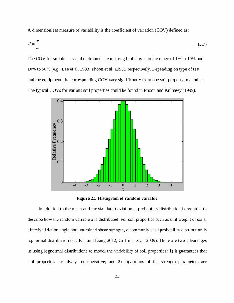
A dimensionless measure of variability is the coefficient of variation (COV) defined as:
(2.7)
The COV for soil density and undrained shear strength of clay is in the range of 1% to 10% and
10% to 50% (e.g., Lee et al. 1983; Phoon et al. 1995), respectively. Depending on type of test
and the equipment, the corresponding COV vary significantly from one soil property to another.
The typical COVs for various soil properties could be found in Phoon and Kulhawy (1999).
Figure 2.5 Histogram of random variable
In addition to the mean and the standard deviation, a probability distribution is required to
describe how the random variable x is distributed. For soil properties such as unit weight of soils,
effective friction angle and undrained shear strength, a commonly used probability distribution is
lognormal distribution (see Fan and Liang 2012; Griffiths et al. 2009). There are two advantages
in using lognormal distributions to model the variability of soil properties: 1) it guarantees that
soil properties are always non-negative; and 2) logarithms of the strength parameters are
-4 -3 -2 -1 0 1 2 3 40
0.1
0.2
0.3
0.4
x
Rel
ati
ve
Fre
qu
ency
24
normally distributed. Two parameters, namely µlnx and ζlnx, are needed to define a lognormal
distribution. The two parameters are related to the mean µx and the standard deviation ζx in the
following equations:
2
ln 2ln 1 x
x
x
(2.8)
2
ln lnln 0.5x x x (2.9)
With the distribution parameters, the probability density function of the lognormal distribution is
written as
2
ln
ln ln 2
lnln
ln1 1, exp
22
x
x x
xx
xf x
x
(2.10)
From Equaiton (2.10), it can be seen that the logarithm of a lognormal variable follows normal
distribution with mean = µlnx and standard deviation = ζlnx. It should be noted that other
probability distributions such as the normal distribution are potential choices for modeling soil
properties.
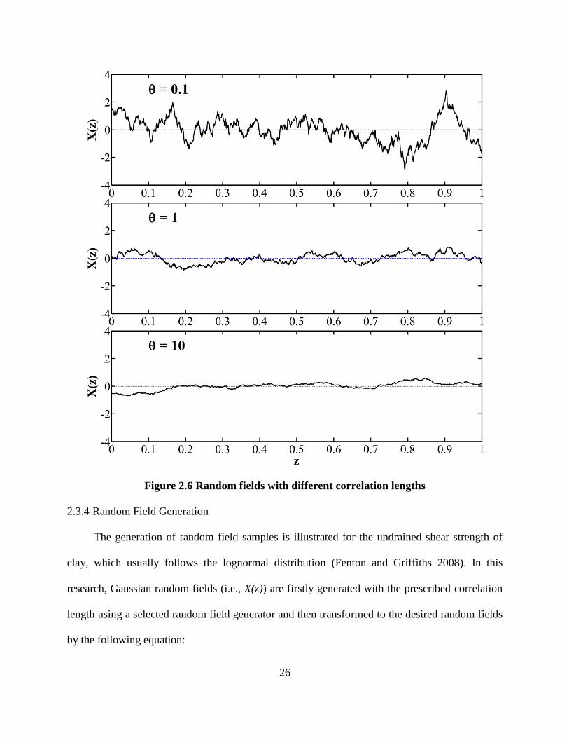
2.3.3 Correlation Function
Soil properties are spatially varying. As a result, soil properties should be modeled as
random fields. In addition to the mean and the variance, a third parameter called correlation
length θ was suggested by Vanmarcke (1977) to characterize the spatial variability of a random
variable. The correlation length is needed to define a correlation function, which describes how
random variables are correlated at different separation distances. For example, the correlation
function for Markov process is given below
2
exp
(2.11)

25
where ρ(η) is the correlation coefficient at the separation distance of η, and θ is the correlation
length. Equation (2.11) says the correlation coefficient decays exponentially with increasing
separation distance. As a measure of the spatial correlation, the correlation length is essential in
the definition of correlation function. A longer correlation length implies that the underlying
random field is more uniform. If the correlation length is short, the underlying random field
varies more rapidly. The following equation shows the covariance function for a stationary
process:
2
xC (2.12)
where ζx is the standard deviation of the random variable at the point level. For simplicity, the
correlation structure of soil properties is modeled as Markovian in this study so that Equation
(2.11) and Equation (2.12) are employed to characterize the spatial variability of soil properties.
26
Figure 2.6 Random fields with different correlation lengths
2.3.4 Random Field Generation
The generation of random field samples is illustrated for the undrained shear strength of
clay, which usually follows the lognormal distribution (Fenton and Griffiths 2008). In this
research, Gaussian random fields (i.e., X(z)) are firstly generated with the prescribed correlation
length using a selected random field generator and then transformed to the desired random fields
by the following equation:

27
( ) exps z X z (2.13)
where s(z) denotes the soil property at the depth z. Common methods for generating random
fields include fast Fourier transform (FFT), local averaging subdivision (LAS), and covariance
matrix decomposition (CMD). In this research, LAS is implemented to generate the random field
samples, mainly because LAS is a fast and accurate method of producing random fields. The
concept of local average subdivision was originated from the fact that quite a number of
engineering measurements are the local averages of the properties under consideration. The
algorithm used in this research to generate one-dimensional Gaussian random process is briefly
described as follows:
1. Generate a random number to represent the global average, with the mean and variance
obtained through the local averaging process theory.
2. Divide the process under consideration into two equal parts, and generate two random
values that can preserve the local average of the parent cell to represent the local average
of each cell. The two values are properly correlated with adjacent cells and exhibiting the
variance according to the local averaging process theory.
3. Subdivide each cell into two equal parts and generate two random values to represent the
local average of each part. Again, the two values have to preserve the local average of the
parent cell. They are also required to be properly correlated with adjacent cells and
exhibiting variance according to local averaging process theory.
4. Repeat Step 3 until the cell at the desired resolution is obtained.
Simply speaking, random fields in LAS are constructed recursively by subdividing the
parent cell into equal parts. More technical details of generating random fields could be found in
Fenton and Griffiths (2008). In this research, the size of local averaging process at the cell level

28
is chosen to be the same as the length of each drilled shaft segment, which is determined by the
load transfer numerical methods. The corresponding load transfer curves (i.e., p-y curves, t-z
curves and q-w curves) are constructed using the trend lines shown in Figure 2.3 and the
randomly-generated soil properties are used as input.
2.4 Reliability Based Design
The reliability-based design methodologies for foundations have become increasingly
popular. Just to name a few for example, multiple resistance factor design (MRFD) for shallow
foundations for transmission line structures was developed based on the first order reliability
method (Phoon et al. 2003a). The MRFD methodology was shown to achieve a more uniform
level of safety compared with applying a single resistance factor. An expanded reliability-based
design approach for drilled shafts based on Monte Carlo simulation (MCS) was proposed (Wang
et al. 2011). The expanded reliability-based approach was not only robust and flexible, but it also
is capable of addressing some of the deficiencies in load and resistance factor design. A quantile-
based approach for calibrating reliability-based partial factors was proposed (Ching and Phoon
2011). In the proposed quantile-based method, the capacity is not required to lump into a single
random variable in the LRFD format, nor is the mathematical optimization in the MRFD format
required. The popularity of RBD methodologies was primarily driven by the desire to achieve a
safe yet economical design in a rational way. It was noted that the geotechnical engineering
community is known to be deep into empiricism (Phoon and Kulhawy 2005) and semi-empirical
or empirical models are widely used. Nevertheless, the underlying assumptions for these models
may not be always satisfied; therefore, the predictions based on the underlying assumptions are
prone to errors. In addition, the soil properties used in geotechnical designs, such as shear
strength and friction angle, are typically inherently difficult to quantify and thus uncertain to

29
some extent. As there are various uncertainties involved in the design models and soil parameters,
it is still highly desirable to develop and implement the RBD methodologies that would enable
the practicing engineers to design foundations rationally.
2.4.1 Multiple Resistance Factor Design
As mentioned earlier, LRFD has some deficiencies. Recent efforts in mitigating the
fundamental flaws of LRFD approach include the work by Phoon et al. (1995, 2003a, 2003b) in
which multiple resistance factor design (MRFD) for transmission line foundation structures was
proposed. In MRFD, the uncertainties of the component resistance are separated and different
resistance factors are applied to different component resistance. The rationale behind the MRFD
is that different components of resistance have different magnitudes of uncertainty. As a result,
the resistance factors for different components of resistance should be different. The main
advantage of MRFD over LRFD is that a more consistent level of reliability can be achieved
(Phoon et al. 2003a, 2003b).
In contrast, the resistance factors in the MRFD are implemented independently of the soil
strata that are possibly present at the site. Consequently, MRFD is unable to achieve a consistent
level of safety (Ching et al. 2013). In reality, it is common that multiple soil strata are present,
and the thickness of each soil stratum may be different. Furthermore, the variability of various
soils would also be different. If constant resistance factors are applied without considering the
thickness and the variability of each soil stratum, it is likely that the resistance factors will be
conservative for one site and unconservative for another site. This is understandable, because the
variability of the resistance of a soil stratum is not only related to the soil properties of the
stratum, but also related to the thickness of the soil stratum. Moreover, the geological

30
stratifications along the depth would matter, since the stratifications have different stiffnesses
and can affect the load transfer.
Therefore, the strategy of implementing constant resistance factors is not able to achieve
the desired consistent level of reliability. The study in Ching et al. (2013) indicates that the
resistance factors should be calibrated considering the variability of each component resistance.
2.4.2 Monte Carlo Simulation–Based Approach
Wang et al. (2011) developed a more general reliability-based design approach for drilled
shafts under axial loading. This approach formulates the design process as an expanded
reliability problem in which Monte Carlo simulation is employed. The approach has a number of
advantages over LRFD: 1) it enables designers to make adjustments on the target reliability
index to accommodate specific needs for particular projects; 2) the process is transparent,
enabling designers to gain insights on how the performance level changes as the pile diameter or
penetration length changes; and 3) the estimate of probability of failure is accurate as long as the
number of samples is large enough.
In this approach, the soil properties along the depth are modeled as independent random
variables. The shortcoming of such a model is that the spatial correlation of soil properties
cannot be accounted for. Note that the spatial correlation of soil properties is important in
reliability analysis. As demonstrated in Griffiths (2009), it can lead to unconservative design if
the dependence structure of soil properties is not considered in the reliability analysis.
2.4.3 Recognition of Soil Spatial Variability
Soil parameters are spatially variable, and the influence of soil spatial variability has
attracted considerable attention. Griffiths et al. (2009) demonstrated a slope stability case in
which ignoring soil spatial variability may lead to unconservative designs. Klammler et al. (2010)

31
demonstrated that the resistance factor in LRFD for a single drilled shaft is affected by soil
spatial variability. More importantly, the resistance factors may be increased if the dependence
structure of soil properties is taken into account. Luo et al. (2012) found that the reliability
against basal heave for braced excavations is significantly influenced by soil spatial variability.
As the spatial variability of soil parameters may affect the reliability of designs, it should be
taken into account in reliability-based analysis.
2.5 Concluding Remarks
The objective of this research is to develop a novel reliability-based design methodology
for deep foundations. The novel methodology consists of the following components:
1. Deterministic models for calculating the response of the pile under axial and lateral
loads;
2. Monte Carlo simulation;
3. Evaluation of the probability of failure.
Although the p-y method and the t-z model have reasonably good accuracy, the results
given by the two methods still have some variations because of the aforementioned uncertainties.
Thus, it is highly desirable to develop a novel RBD methodology that can consider these
uncertainties. In the proposed methodology, the p-y method and the t-z model are still used as
numerical algorithms to evaluate the response of the pile to external loads. In addition to the p-y
method and the t-z model, Monte Carlo simulation techniques are incorporated into the
computational tools, so that various sources of uncertainties can be taken into account in the p-y
method and the t-z model.
It is worth noting that soil properties are modeled as random fields. The advantage of using
random field modeling is that the spatial variability of soil properties can be considered in the

32
reliability analysis. So far, the current LRFD approach has not considered the spatial variability
of soil properties. Consequently, the design according to the LRFD approach might be
potentially unconservative, as the variability of the related soil properties is not modeled
correctly. On the other hand, this deficiency could be addressed in the proposed methodology.
More importantly, performance based design is implemented in the proposed methodology.
The advantage of using performance-based design approach is that various sources of
uncertainties can be considered consistently in both strength limit states and serviceability limit
states. In contrast, the current LRFD approach is still deterministic for the serviceability limit
state.
Furthermore, the system reliability of a design can be considered in the proposed
performance-based design. In the developed methodology, not only are the individual limit states
considered in the design but also the system failure is considered as well. The advantage of
taking system failure events into account is that a more reliable design can be achieved.

33
CHAPTER 3. LATERALLY LOADED PILES
3.1 Introduction
In the current LRFD approach given in the AASHTO (2010) specifications, various
resistance factors corresponding to different design methods have been provided for various
strength limit states. However, there is an unresolved issue in the current AASHTO
specifications in that the service limit check of a drilled shaft or driven pile is still carried out as
in the Level I allowable stress approach. Unfactored loads are used to evaluate the deformation
response of deep foundations using the deterministic computational models. The uncertainties
arising from various sources, such as soil properties and their spatial variations, cannot be
systematically taken into account. To provide a consistent framework for checking both strength
limits and service limits, a Level III reliability-based design method for drilled shafts subjected
to lateral loads is presented in this research.
The objective of this research is to present a performance-based reliability method and the
associated computational algorithms for a laterally loaded drilled shaft or driven pile using a
sampling-based approach. In the proposed approach, input to the computational model for the
nonlinear soil structure interaction problem, such as p-y curves, is treated as random variables. In
particular, soil properties, such as strength parameters, soil modulus (or subgrade reaction
modulus), and unit weight, are modeled as random fields to account for the spatial variability and
spatial correlations. The statistical parameters, including the mean, variance, and correlation
length, are used to characterize a stationary random field. Random samples of the input are

34
generated according to the prescribed probability distributions. The deflection of the drilled shaft
subjected to lateral loads is evaluated for each set of samples. In each realization, if the shaft
head deflection exceeds the specified allowable value, then it is considered as an event of
unsatisfactory performance. Consequently, the probability of failure (i.e., unsatisfactory
performance) Pf, is simply calculated as the ratio of the number of events of unsatisfactory
performance to the total number of realizations of random input. The design parameters of a deep
foundation (i.e., shaft diameter D and shaft length L) are determined such that the desired target
reliability level is met. A computer program, called Probabilistic Laterally Loaded Piles (P-
LPILE), was developed by the authors to facilitate the computation according to the described
sampling-based algorithms. The calculation of the deflection of a drilled shaft subjected to lateral
loadings is based on the commonly-used p-y method (Reese 1977). A design example is given to
demonstrate the application of the proposed methodology.
3.2 Numerical Algorithm for Analyzing Laterally Loaded Drilled Shafts
In the analysis of a laterally loaded drilled shaft, the widely used p-y method will be used
as a numerical algorithm to calculate the response of a laterally loaded pile. The detailed
discussion of the p-y method can be found in Chapter 2. It is noted that the non-linear EI-moment
relationship is taken into account when calculating the displacement of the pile. The analytical
method in Reese et al. (2004) is adopted for calculating the relationship between the bending
moment and the flexural stiffness EI.
3.3 Probabilistic Load Description
The design loads applied to the foundations are uncertain to some degree. According to
Nowak and Collins (2000), coefficients of variation for dead load could range from 0.08 to 0.10
35
for buildings and bridges, while those for live load including sustained live load and transient
live load could range from 0.18 to 0.89. Previous investigations (e.g., Ellingwood and Tekie
1999; Ellingwood et al. 1980) have found that normal, lognormal, gamma, Type-I and Type-II
Gumbel distributions are possible choices to statistically characterize load models. For example,
the maximum live load for a structure can be statistically characterized by Type-I Gumbel
distributions, while sustained live load can be modeled as a gamma distributed random variable.
3.4 Model Uncertainty
Model uncertainty is always present, as any computational model is an idealization or
simplification of real-world conditions. The method for accounting for this uncertainty is
described below. Suppose Yp denotes the prediction based on a model, and NM is a bias factor
that describes the model uncertainty, then the actual behavior denoted as Ym can be related to the
prediction and bias as follows:
m M pY N Y (3.1)
It is noted that the error term NM is a random variable whose statistical characters can be
described as normal or lognormal distributions (e.g., Kung et al. 2007; Phoon and Kulhawy
2005).
In the p-y method, the soil reaction to lateral loading is modeled by p-y curves. To account
for the uncertainty of the p-y curves, a random variable is generated in each simulation according
to the prescribed probability distribution of the bias factor and is used to correct the soil reaction
predicted by the p-y curve. As shown in Equation (3.1), the product of the generated bias factor
and the prediction is viewed as the true soil reaction.

36
3.5 Performance-Based Reliability Analysis
3.5.1 Performance-Based Design
In current LRFD practices, strength limit states and service limit states are considered for
various combinations of load effects. Appropriate load and resistance factors are applied to check
that the design satisfies both limit states. The final design would be governed by either strength
limit states or service limit states. However, as mentioned earlier, the service limit check for
laterally loaded drilled shafts in the current AASHTO guidelines uses the traditional ASD
approach, in which the load factor and the resistance factor are taken as unity and the
deterministic p-y method (e.g., the LPILE program) is utilized for calculating the deflection of
the foundation under lateral loads. As noted in Zhang and Ng (2005), currently serviceability
limits are still considered using a conventional deterministic approach in most limit state design
codes. The uncertainties arising from various sources (such as soil variability and load
uncertainty) cannot be accounted for. Therefore, there is an obvious inconsistency in the design
for considering the strength limits and service limits. To address this deficiency, a transition to
the performance-based design (PBD) approach would be desirable, a viewpoint that is also noted
by Nowak and Collins (2000). In the proposed framework, performance-based criteria can be
established as the objectives for deep foundation design. The performance criteria are expressed
in terms of allowable deflections of the foundation structures subjected to the design loads. In the
PBD methodologies, a foundation design would be satisfactory provided the specified
performance criteria are satisfied for the prescribed load effects.
3.5.2 Probability of Unsatisfactory Performance
The performance criteria of the proposed approach for laterally loaded shafts are stated in
terms of the shaft head deflection. Failure is said to occur if the shaft head deflection exceeds the

37
allowable limits or if the numerical algorithm is unable to converge. Based on the described
performance criteria, a general form for the probability of failure can be formulated as follows:
0
( )f t a t a
G
p P y y f d I y y f d
x x x x (3.2)
where yt is the shaft-head deflection, ya is the allowable displacement specified by the
performance criteria, F is the failure region, I[∙] is the indicator function, x is a vector of input
and f(x) is the joint probability density function. The indicator function in Equation (3.2) is equal
to 1.0 if yt is equal to or greater than ya. It is zero for other conditions. The design objective can
be written as:
f TP P (3.3)
where PT is the target probability of failure. The design objective is therefore to optimize a deep
foundation dimension so that the computed probability of failure Pf is equal to or less than the
target probability of failure.
The determination of the target reliability is not an easy task. It involves the consideration
of the consequence of failure, the construction costs, and the design life of the system under
consideration, among others. A number of factors such as economic issues, social effects, and the
existing levels of technology may have to be considered in order to determine an appropriate
target probability of failure. It is noted that most civil engineering systems have a target
probability of failure between 1/1000 and 1/100,000 (Fenton and Griffiths 2008). According to
AASHTO (2010), a reliability index of 2.3 (approximately, Pf = 1/100) is used for shaft groups,
while a reliability index of 3.0 (approximately, Pf = 1/1000) or higher is used for a single drilled
shaft.

38
3.5.3 Sampling-Based Method
In the context of laterally loaded shafts, the reliability analysis simply becomes the
evaluation of the failure probability defined in the previous section. In general, it is preferable to
evaluate the integral expressed in Equation (3.2) analytically. Nevertheless, it is quite difficult to
evaluate this integral directly for the following reasons: 1) f(x) is a multivariate function for input
vector x, which may be of high dimensions; 2) it is hard to determine the failure region (i.e. F),
particularly for a nonlinear soil structure interaction for which no analytic equation exists that
can accurately predict the response of a drilled shaft under the lateral loads. The Monte Carlo
integration (Robert and Casella 2004) is a realistic alternative for evaluating the integral.
Monte Carlo simulation (MCS) is a standard statistical method in which the response of a
complex system is calculated repeatedly using a sequence of the generated random samples as
input. The Monte Carlo approach of evaluating the probability of failure is expressed as follows:
1
1 n
f i t a
i
P I y yn
(3.4)
where n is the number of samples. By the law of large numbers, the unbiased estimator for Pf
expressed in Equation (3.4) converges to the exact value as n→inf with a probability of 1.0. The
Monte Carlo statistical method offers several advantages: 1) the Monte Carlo method gives the
unbiased estimate of the probability of failure; 2) the accuracy of the estimate increases with
increasing n; and 3) the method is mathematically simple. The accuracy of the estimate can be
evaluated by its coefficient of variation, which can be estimated by the following equation:
2
1
1
1
n
f i t a f
if
P I y y Pn n P
(3.5)
The flow chart for the proposed approach using the Monte Carlo technique is presented in
Figure 3.1. The objective of the approach is to find feasible foundation dimensions (i.e., D and L)
39
that are able to achieve the target reliability for the prescribed performance criteria and design
loads. In the proposed framework, a deterministic computational method is coupled with Monte
Carlo simulation techniques in which the uncertainties of soil properties are quantified by field
means, field variances, and the correlation structures. For loads and model errors, the probability
distributions, mean values, and variances should be determined. For each trial foundation
dimension, the probability of failure (unsatisfactory performance) is evaluated. The design
process entails finding the optimum foundation dimension that is economical while meeting the
reliability requirements. A computer program named P-LPILE was developed to incorporate the
p-y method and the Monte Carlo simulation techniques described in this research.

40
Figure 3.1 Flow chart of the proposed method
3.6 Design Example
Consider an example presented in a recent FHWA report (Brown et al. 2010). As shown in
Figure 3.2, a drilled shaft is to be designed in a very stiff clay site with the design loads of 111.2

41
kN (i.e., 25 kips) in shear and 677.9 kN∙m (i.e., 500 kip-ft) in moment applied at top of the
drilled shaft on the ground level. The p-y curve for stiff clay (Reese et al., 2004) without free
water was used in the report to represent the lateral soil–pile interaction. For generating the p-y
curves, the mean values of the pertinent soil properties are as follows: the undrained shear
strength is 103.4 kPa (i.e., 15 psi), the unit weight is 19 kN/m3 (i.e., 0.07 pci), and the strain
corresponding to 50% of the maximum principle stress difference (ε50) is 0.005. The probability
distributions of these soil properties are assumed to be lognormal. The example in the FHWA
report does not provide values for COV for soil properties; therefore, the following COV values
are assumed: a COV for undrained shear strength of 40%, a COV for ε50 of 20%, and a COV for
effective unit weight of 4%. The maximum allowable lateral deflection at the shaft head was
given in the FHWA report as 12.7 mm (i.e., 0.5 inch), which is deterministic. For calculating the
Young’s modulus of concrete, the compressive strength of concrete (31027.5 kPa, 4500 psi) is
used. The properties of the reinforcing steels are as follows: the yield strength is 413700 kPa (i.e.,
60,000 psi), and the elastic modulus of steel is 200 GPa (29,000 ksi). These values are used to
calculate the values of EI of the drilled shaft as a function of the bending moment (see Reese et
al. 2004). In the FHWA report, a resistance factor of 0.67 was used in the strength limit check for
determining the foundation size, while the computer program LPILE was used to calculate the
lateral deflection of the drilled shaft head under the unfactored loads at the pile head. The
foundation dimension of 1.22 m (i.e., 4 ft) in diameter and 6.10 m (i.e., 20 ft) in length, with a
total of 12 No. 11 rebars and a cover of 7.62 cm (3 in), was used for the final design according to
the current LRFD methodologies documented in the FHWA report. This design is re-examined
herein using the P-LPILE computer program and the proposed approach. Three soil parameters,
namely ε50, the undrained shear strength (denoted as Su), and the effective unit weight (denoted

42
as γ'), are required to construct the p-y curve. For clarity, the correlation lengths for undrained
shear strength, ε50, and effective unit weight are denoted as θln(Su), θln(ε50) and θln(γ'), respectively.
The correlation lengths of soil parameters are varied in a typical range to investigate their
influences on the computed probability of failure.
Figure 3.2 Example of a drilled shaft
3.6.1 Influence of Incremental Length
The random soil properties are generated using local averaging subdivision (LAS). The
sensitivity of the computed probability of failure as affected by the unit cell length of the LAS is
investigated in this section. The unit shaft length in the numerical p-y computational algorithm
(denoted as h) is also set as the cell length for LAS; the number of segments is set to 400, 200,
43
100, and 50 in the sensitivity analysis. The corresponding ratio of h over D is 0.0125, 0.025, 0.05,
and 0.1 for a diameter of 1.22 m (4.0 ft). Failure is said to occur when the lateral deflection at the
top of the drilled shaft exceeds 12.7 mm (0.5 in). Figure 3.3 shows the relationship between pf
and the unit shaft length when the correlation length of undrained shear strength is varied from 2
m (6.56 ft) to 64 m (209.97 ft), while keeping θln(ε50) equal to 1.0 m (3.28 ft) and θln(γ') equal to
1.0 m (3.28 ft). Figure 3.4 shows the relationship between Pf and the unit shaft length as the
correlation length of ε50 is varied from 2 m (6.56 ft) to 64 m (209.97 ft), while fixing both θln(Su)
and θln(γ') at 1.0 m (3.28 ft). Similarly, Figure 3.5 shows the relationship between Pf and the unit
shaft length as the correlation length of unit weight is varied from 2 m (6.56 ft) to 64 m (209.97
ft), while fixing both θln(Su) and θln(ε50) at 1.0 m (3.28 ft). It can be seen from these three figures
that Pf does not vary, regardless of the number of segments used in the p-y method. Therefore,
the selection of the unit shaft length can be determined based on the computational algorithm of
the p-y method rather than the LAS method. A unit shaft length on the order of 10% of the
drilled shaft diameter can be conveniently selected for numerical computation. It can also be
observed from these three figures that the computed probability of failure for various correlation
lengths of ε50 and γ' is about the same. On the other hand, the computed probability of failure for
different correlation lengths of undrained shear strength is significantly different. This finding
highlights the importance of considering the correlation length of undrained shear strength in the
reliability analysis.
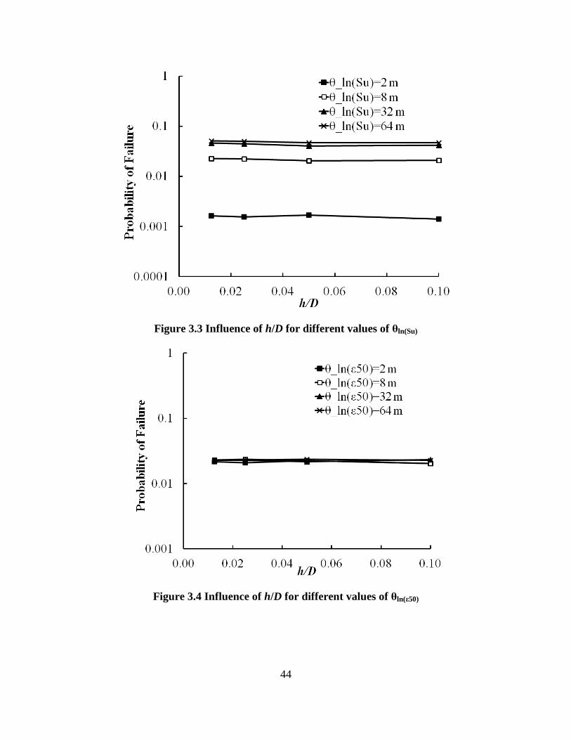
44
Figure 3.3 Influence of h/D for different values of θln(Su)
Figure 3.4 Influence of h/D for different values of θln(ε50)

45
Figure 3.5 Influence of h/D for different values of θln(γ’)
(Note: 2 m =6.56 ft; 8 m = 26.25 m; 32 m = 104.99 ft; 64 m = 209.97 ft.)
3.6.2 Realizations of the Drilled Shaft Head Displacement
In this section, the influences of θln(Su) on the realization of the computed drilled shaft
deflection are discussed. As mentioned earlier, the correlation length of undrained shear strength
could exert significant influence on the computed probability of failure based on the specified
performance criterion (i.e., 12.5 mm (0.5 in) lateral deflection at the top of the drilled shaft).
Figure 3.6 shows the histograms of the drilled shaft-head deflection yt for different correlation
lengths of shear strength ranging from 0.1 m (0.33 ft) to 64 m (209.97 ft), while keeping the
values of correlation length for both ε50 and γ' as 1.0 m (3.28 ft). The means and the standard
deviations of yt denoted as μyt and ζyt are plotted in the histograms. It can be seen that the means
and standard deviations of yt are noticeably different for different correlation length of undrained
shear strength. This finding indicates that the mean and the standard deviation of yt are clearly
sensitive to the spatial variability of shear strength. Figure 3.7 shows the convergence of the

46
computed Pf using Equation (3.4) for different values of θln(Su). The estimated probabilities of
failure for θln(Su) of 2 m (6.56 ft), 8 m (26.25 ft), 32 m (104.99 ft), and 64 m (209.97 ft) are
0.0016, 0.022, 0.044, and 0.048, respectively. The COVs of these estimates range from 2% to
13%. It is evident that the computed probability of failure is highly dependent upon the
correlation length of undrained shear strength. It can be concluded that the estimate of Pf could
be biased, if the spatial variability (or correlation length) of undrained shear strength is ignored.

47
Figure 3.6 Realizations of the lateral deflection for different values of θln(γ’)
(Note: 1 mm = 0.0394 in and 1 m = 3.28 ft.)

48
Figure 3.7 Convergence of the estimates
(Note: 2 m =6.56 ft; 8 m= 26.25 ft; 32 m = 104.99 ft; 64 m = 209.97 ft.)
3.6.3 Influence of Variability of Soil Properties
The variability of soil properties is characterized by COV and correlation length. The
effects of varying COV and correlation length of the undrained shear strength for the design
example are shown in Figure 3.8. In the sensitivity analysis, both θln(ε50) and θln(γ') are set to 1.0 m
(3.28 ft), while the COVs of ε50 and γ' are set to 20% and 4%, respectively. It can be seen that Pf
increases with increasing COV of undrained shear strength. In addition, Pf varies significantly
with different θln(Su).

49
Figure 3.8 Influence of the spatial variability of Su
(Note: 0.2 m =0.66 ft; 0.5 m = 1.64 ft; 1 m = 3.28 ft; 4 m = 13.12 ft; 8 m= 26.25 ft; 32 m =
104.99 ft; 64 m = 209.97 ft.)
The design outcome in the FHWA report is re-examined by means of the P-LPILE
program, in which the effects of COV and correlation length of undrained shear strength are
varied as shown in Table 3.1. The other relevant parameters are set as follows: both θln(ε50) and
θln(γ') are set to 1.0 m (3.28 ft), while the COV of ε50 and γ' are set to 20% and 4%, respectively.
For the selected PT =0.001, it can be seen that FHWA design may not be satisfactory for cases
where the COV and correlation length of undrained shear strength are large. For example, if θln(Su)
is equal to 1.0 m (3.28 ft) and the COV of undrained shear strength is equal to 60%, the
foundation dimension is unsatisfactory.
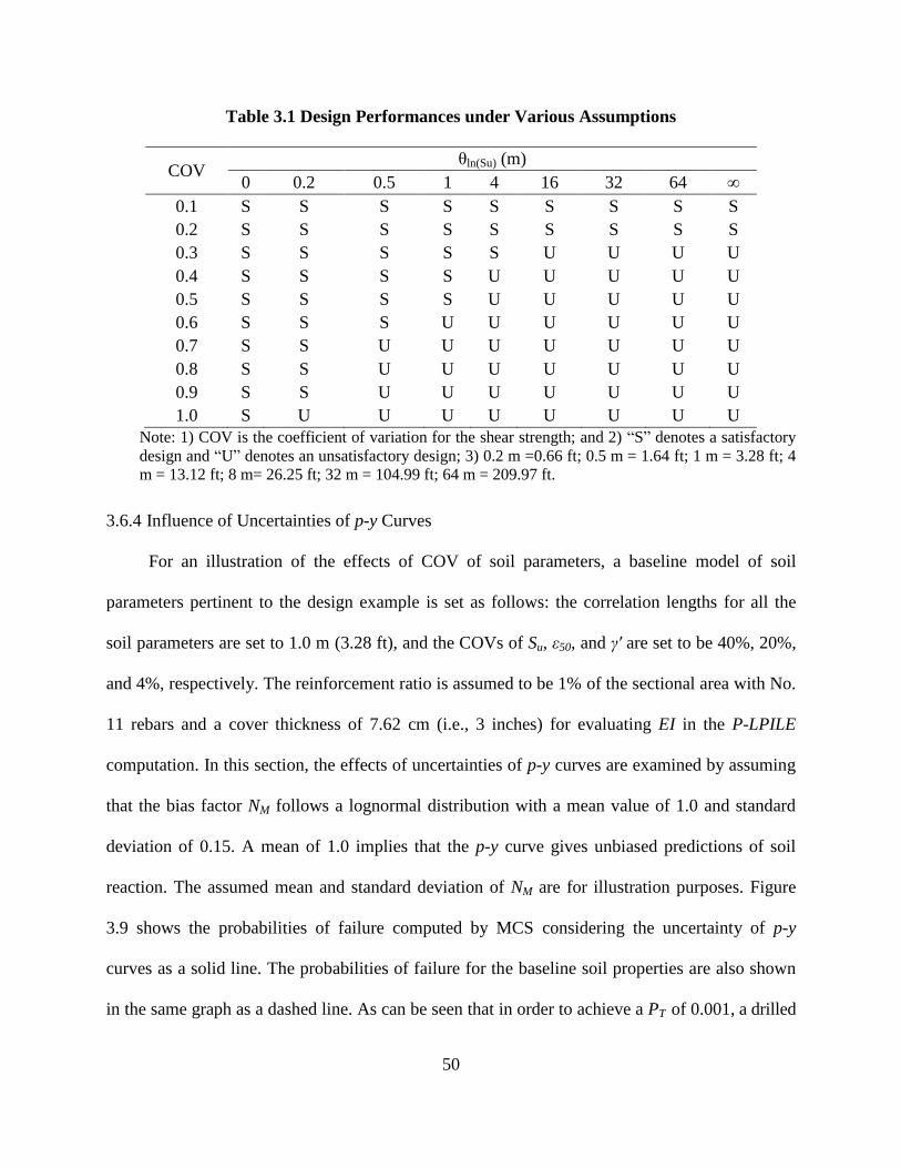
50
Table 3.1 Design Performances under Various Assumptions
COV θln(Su) (m)
0 0.2 0.5 1 4 16 32 64 ∞
0.1 S S S S S S S S S
0.2 S S S S S S S S S
0.3 S S S S S U U U U
0.4 S S S S U U U U U
0.5 S S S S U U U U U
0.6 S S S U U U U U U
0.7 S S U U U U U U U
0.8 S S U U U U U U U
0.9 S S U U U U U U U
1.0 S U U U U U U U U
Note: 1) COV is the coefficient of variation for the shear strength; and 2) ―S‖ denotes a satisfactory
design and ―U‖ denotes an unsatisfactory design; 3) 0.2 m =0.66 ft; 0.5 m = 1.64 ft; 1 m = 3.28 ft; 4
m = 13.12 ft; 8 m= 26.25 ft; 32 m = 104.99 ft; 64 m = 209.97 ft.
3.6.4 Influence of Uncertainties of p-y Curves
For an illustration of the effects of COV of soil parameters, a baseline model of soil
parameters pertinent to the design example is set as follows: the correlation lengths for all the
soil parameters are set to 1.0 m (3.28 ft), and the COVs of Su, ε50, and γ' are set to be 40%, 20%,
and 4%, respectively. The reinforcement ratio is assumed to be 1% of the sectional area with No.
11 rebars and a cover thickness of 7.62 cm (i.e., 3 inches) for evaluating EI in the P-LPILE
computation. In this section, the effects of uncertainties of p-y curves are examined by assuming
that the bias factor NM follows a lognormal distribution with a mean value of 1.0 and standard
deviation of 0.15. A mean of 1.0 implies that the p-y curve gives unbiased predictions of soil
reaction. The assumed mean and standard deviation of NM are for illustration purposes. Figure
3.9 shows the probabilities of failure computed by MCS considering the uncertainty of p-y
curves as a solid line. The probabilities of failure for the baseline soil properties are also shown
in the same graph as a dashed line. As can be seen that in order to achieve a PT of 0.001, a drilled

51
shaft of L = 6 m (19.68 ft) and D ≥ 1.2 m (3.94 ft), or L ≥ 7 m (22.97 ft) and D ≥ 1.1 m (3.61 ft)
would be sufficient for the baseline soil properties. However, if the uncertainty of the p-y curves
is considered, the foundation dimensions for the feasible design would be L = 6 m (19.68 ft) and
D ≥ 1.3 m (4.27 ft), or L ≥ 7 m (22.97 ft) and D ≥ 1.2 m (3.94 ft). Therefore, the uncertainties of
p-y curves have resulted in a larger foundation dimensions for the same soil properties and
design loads.
Figure 3.9 Influence of uncertain p-y curves
(Note: 1 m = 3.28 ft; 2 m = 6.56 ft; 6 m = 19.68 ft; 7 m 22.97 ft; 8 m = 26.25 m; 9 m = 29.53 ft.)
3.6.5 Influence of Uncertainties of Loads
As discussed previously, sustained live loads can be modeled as a gamma-distributed
random variable. In this section, it is assumed that the shear force applied at top of the drilled
shaft is a gamma-distributed variable with a mean of 111.2 kN (25 kips) and a COV of 30%. In
addition, it was assumed that the bending moment at the top of the drilled shaft is proportional to

52
the shear force. The probabilities of failure computed by MCS for the assumed uncertain loads
under the same soil conditions are shown in Figure 3.10, with the Pf values for the baseline soil
properties depicted as a dashed line. It can be seen that the feasible foundation dimensions would
be L = 6 m (19.69 ft) and D ≥ 2.1 m (6.89 ft), L = 7 m (22.97 ft) and D ≥ 1.6 m (5.25 ft), or L ≥ 8
m (26.25 ft) and D ≥ 1.4 m (4.59 ft). The feasible foundation sizes with the consideration of load
uncertainty are larger than for those that do not consider the load uncertainties.
Figure 3.10 Influence of uncertain loads
(Note: 1 m = 3.28 ft; 2 m = 6.56 ft; 6 m = 19.68 ft; 7 m 22.97 ft; 8 m = 26.25 m; 9 m = 29.53 ft.)
3.6.6 Influence of Cross-correlation
A parametric study is conducted to investigate the influence of cross-correlation. In the
parametric study, the COVs of Su, ε50, and γ' are set as 45%, 20%, and 4%, respectively. The
correlation lengths of both ε50 and γ' are set at 1.0 m (3.28 ft), while θln(Su) is varied. It is believed
that the cross-correlation between the unit weight and the undrained shear strength (ε50) is largely
minimal. Only the cross-correlation between undrained shear strength and ε50 is considered. The

53
Pearson linear correlation coefficient is used to measure the cross-correlation that is defined with
respect to logarithms of both variables. Figure 3.11 shows the influence of the cross-correlation
between Su and ε50 for a drilled shaft with a 1.10-m (3.61 ft) diameter and 8.0-m (26.25 ft) length.
It is clear that the probability of failure exhibits significant variation for different cross-
correlations. This finding indicates that the cross-correlation should be considered in order to
have an accurate evaluation for the failure probability.
Figure 3.11 Influence of the cross-correlation
(Note: 2 m = 6.56 ft; 5 m = 16.40 m; 8 m = 26.25 m.)
3.7 Summary and Conclusions
In this chapter, a performance-based reliability method that considers the spatial variability
of soil properties for a laterally loaded drilled shaft was presented. The spatial variability of soil
properties is considered by using random field theories. The random field of a soil parameter is
statistically characterized by the field mean, field variance, and the correlation structure. In

54
addition, uncertainties of the applied loads and the computational models can also be accounted
for using Monte Carlo simulation according to the prescribed probability distributions. The
performance criteria for the laterally loaded drilled shaft are stated in terms of the lateral
deflection at the top of the pile. Failure, or unsatisfactory performance, is defined as the event
that the pile-head deflection exceeds the allowable displacement. A computation program called
P-LPILE was developed that incorporates the Monte Carlo simulation techniques and the p-y
method for computing the reliability of the laterally loaded drilled shafts. Based on the numerical
results presented in this research, the following conclusions can be made:
1. The spatial variability of soil properties, particularly the COV and correlation length of
the undrained shear strength for cohesive soils, could exert significant influence on the
computed probability of failure for the specified performance criteria. The difference in
the computed probability of failure caused by different correlation lengths of Su could be
several orders of magnitude. Additionally, the cross-correlation between Su and ε50 is
critical in the evaluation of the failure probability. The failure probability would be
biased if the cross-correlation is not considered.
2. Apart from soil spatial variability, the proposed approach provides a systematic
procedure to consider uncertainties due to the computational model and applied loads. A
random bias factor is introduced to account for the uncertainty of p-y curves. The
estimated probability of failure increases if the uncertainty of the adopted p-y curves is
considered. The uncertainty of loads is considered by sampling from their probability
distributions and using the samples as input. The calculated probability of failure
increases when the uncertainty of loads is considered.

55
3. The proposed approach is useful for conducting reliability analysis to check the
serviceability limit in the current LRFD framework. Based on the conducted parametric
studies, the reliability for the serviceability limit design of a laterally loaded pile is
sensitive to the spatial correlation of soil properties, soil variability, and the uncertainty
of p-y curves and loads.
4. The proposed approach is very versatile, as it allows practicing engineers to input the
means, variances, and probability distributions of the load model; site-specific soil
properties; and the bias factor for the p-y curves. Furthermore, engineers can specify the
target reliability index according to the intended functions of the structures under
consideration.

56
CHAPTER 4. AXIALLY LOADED PILES
4.1 Introduction
The objective of this chapter is to present a fundamentally sound and robust performance-
based design method for drilled shafts subjected to axial loads. In the performance based design
framework, the input of soil properties in the computational model and the model error are
treated as random variables. Monte Carlo simulation techniques are used to generate a large
number of random samples according to the prescribed probability distributions. Next, the
response of a drilled shaft to random input is evaluated repeatedly using the deterministic
computational models per sample trial. The performance-based acceptance criteria are specified
in terms of the allowable drilled shaft settlement. The computation of the load-settlement curve
of an axially loaded drilled shaft is carried out using the load transfer curves specified in the
current AASHTO guidelines (AASHTO 2010) and a computer code P-TZPILE developed
recently by the authors. Failure is said to occur if the settlement of the shaft head exceeds the
allowable limit. The probability of failure Pf is computed as the ratio of the number of
unsatisfactory results to the total number of samples. In the context of performance-based design,
the basic design parameters such as drilled shaft diameter D and length L can be adjusted to
achieve the desired reliability level to meet the needs of a particular project. Two design
examples are given to illustrate the application of the Monte Carlo simulation algorithms for the
design of an axially loaded drilled shaft. The proposed method not only addresses the current
shortcoming of the LRFD for the service limit check, but it also offers the following advantages:
1) it is conceptually simple and gives an unbiased estimate of the probability of failure; 2) it is a

57
true reliability-based design that explicitly accounts for the uncertainties arising from the input of
computational models and model errors; 3) it can explicitly account for the spatial variance of
soil properties; 4) it is a sampling-based and robust process; and 5) it is project-based, since site-
specific information is used in the reliability analysis.
4.2 Performance-Based Design
It is anticipated that in the future, many code-writing organizations will make a transition
towards performance-based design codes (Nowak and Collins 2000). In the context of
performance-based design (PBD), the design objectives are defined in terms of the allowable or
tolerable displacement of the foundation structures under the design loads. There are several
advantages of using performance-based design. In the traditional design methodologies, the
strength limit state or the ultimate limit state is checked to assure the summation of the load
effects does not exceed the summation of the resistance. However, the interpretation of nominal
resistance can be problematic due to various criteria being suggested for interpreting nominal
resistance from the load settlement curve obtained from the load test (Roberts and Misra 2010).
The use of a performance-based design approach can remove the ambiguity in interpreting
nominal resistance from the load-settlement curve obtained from actual load tests. In traditional
design methodologies, in addition to checking the ultimate limit state or the strength limit state,
the service limit state is also checked to assure the functionality of the structure. Indeed, only one
of the limit states governs the design. If excessive displacement is induced on the structure, the
structure either fails due to the overstress on the materials or is not able to serve the desired
function in a satisfactory manner. Therefore, the adoption of a performance-based design
methodology could eliminate the need to check for both strength limits and service limits.

58
In the probability-based design approaches, the safety of a system is defined in terms of the
probability of failure (Nowak and Collins 2000). For axially loaded drilled shafts, the
performance-based design approach uses the performance criteria stated in terms of the drilled
shaft head settlement. Failure is said to occur when the drilled shaft head settlement exceeds the
specified allowable limit. Then, the probability of failure Pf can be defined as follows:
( )f t a t a
F
P P y y f d I y y f d x x x x (4.1)
where yt is the drilled shaft head settlement, ya is the allowable settlement, F is the failure region,
I[∙] is the indicator function, x is a vector of variables, and f(x) is a joint probability density
function. The indicator function in Equation (4.1) is equal to 1.0 if yt is equal to or greater than ya;
otherwise, it is zero.
4.3 Framework of Reliability-Based Design
In the context of the axially loaded drilled shafts, the reliability analysis simply becomes
an evaluation of the integral expressed in Equation (4.1). In general, it is preferable to evaluate it
analytically. However, it is quite difficult to evaluate this integral directly for the following
reasons: 1) f(x) is a multivariate function for input x which may be correlated or of high
dimensions; 2) it is difficult to determine the failure region (i.e., F), in particular in the context of
the implicit solution involving nonlinear soil-foundation interaction analysis, where an iteration
is involved for force equilibrium and strain compatibility and no analytic equation exists that can
predict the load-displacement curve of a drilled shaft under axial loading. Therefore, the Monte
Carlo integration technique (Robert and Casella 2004) is a realistic alternative to evaluate the
integral.
59
4.3.1 Monte Carlo Simulation
Monte Carlo simulation (MCS) is a standard statistical method in which the response of a
complex system is calculated repeatedly using a sequence of the generated random samples as
inputs (e.g., Ang and Tang 1984; Fenton and Griffiths 2008). More details on Monte Carlo
statistical method can be found elsewhere (e.g., Robert and Casella 2004; Fishman 1996). In
MCS, a large number of random field samples are generated, and each set of samples is used as
input to the developed P-TZPILE computer program. Next, the settlement of a drilled shaft
subjected to axial loads is computed repeatedly until a desired or prescribed sample size is
achieved. With the performance criteria defined (i.e., the allowable drilled shaft head settlement),
it is possible to determine whether or not failure will occur. The Monte Carlo approach for
evaluating the probability of failure, based on the performance criterion, is expressed as follows:
1
1 n
f i t a
i
P I y yn
(4.2)
where n is the number of samples. By the law of large numbers, the estimation for Pf expressed
in Equation (4.2) converges to the exact value as n→inf with the probability of 1.0. There are
several advantages of using the Monte Carlo statistical method: 1) the Monte Carlo method gives
an unbiased estimate of the probability of failure; 2) the accuracy of the estimate increases with
increasing n; and 3) the method is conceptually and mathematically simple. The accuracy of the
estimate can be evaluated by its coefficient of variation (COV), which can be estimated by the
following equation:
2
1
1
1
n
f i t a f
if
P I y y Pn n P
(4.3)
Figure 4.1 shows the flow chart for the performance-based design framework. The purpose
of the design procedure is to find out feasible combinations of basic design parameters (i.e.,
60
diameter D and length L) of a drilled shaft that can provide the target reliability for the specified
performance criteria. It starts with characterizations of the probability distributions of the input
for the computational model. In the next step, the basic design parameters and a sample size are
assumed. To guarantee convergence of the Pf estimate in Equation (4.2), the sample size has to
be sufficiently large. With the assumed foundation dimensions, the response of the foundation to
random input is calculated repeatedly using a different set of randomly-generated samples as
input. If uncertainties of load effects can be characterized probabilistically, the load effects could
also be simulated in the same fashion as the resistance in the proposed framework. The
probability of failure can be evaluated with Equation (4.2) using the resulting output from the
repetitive calculations. The process is executed iteratively by adjusting the foundation
dimensions until the calculated probability of failure is equal to or smaller than the target
probability of failure.

61
Figure 4.1 Flow chart of Performance-Based Reliability Design
The determination of the target reliability is not an easy task. It involves determination of
the consequence of failure, the construction costs, the design life, and so on. A number of factors
such as economic issues, societal effects, and existing technical levels of computational models

62
may have to be considered simultaneously to determine the appropriate target probability of
failure. Previous research (e.g., Phoon et al. 1995) indicates that a reliability index of 3.2 (i.e., Pf
= 6.8714 × 10⁻⁴
) is appropriate for ultimate limit state and 2.6 (i.e., Pf = 0.0047) for the service
limit state. It is noted that most civil engineering systems have a target probability of failure
between 1/1000 and 1/100,000 (Fenton and Griffiths 2008). In this research, for the purpose of
illustration, a target probability of failure of 1/1000 is adopted.
4.3.2 Uncertainties of Soil Properties
Soil properties are needed as inputs to evaluate the load-displacement behavior. As a result,
the variations in the soil properties can directly influence the calculated displacement. Therefore,
it is important to recognize the presence of the underlying uncertainties or risk during the design
process, and it is necessary to quantify the variability of inputs in the reliability-based design. In
this research, soil properties are modeled as random fields to account for the spatial variability.
The detailed discussion of random field modeling and the random field generation can be found
in Chapter 2.
4.3.3 Uncertainties of Model Error
Model error or bias is defined as the ratio of the measured to the estimated, namely:
m
e
Yb
Y (4.4)
where Ym denotes the measured value and Ye denotes the estimated value. In most cases, the
computational models used to represent the reality do not produce a bias of 1.0 due to the
simplifications and the imperfect knowledge regarding the soil-foundation interaction. For the
axially loaded drilled shaft, the underlying assumption is that the soil–drilled shaft interaction
behavior is known and could be modeled using the load-transfer curves. In the past, a number of
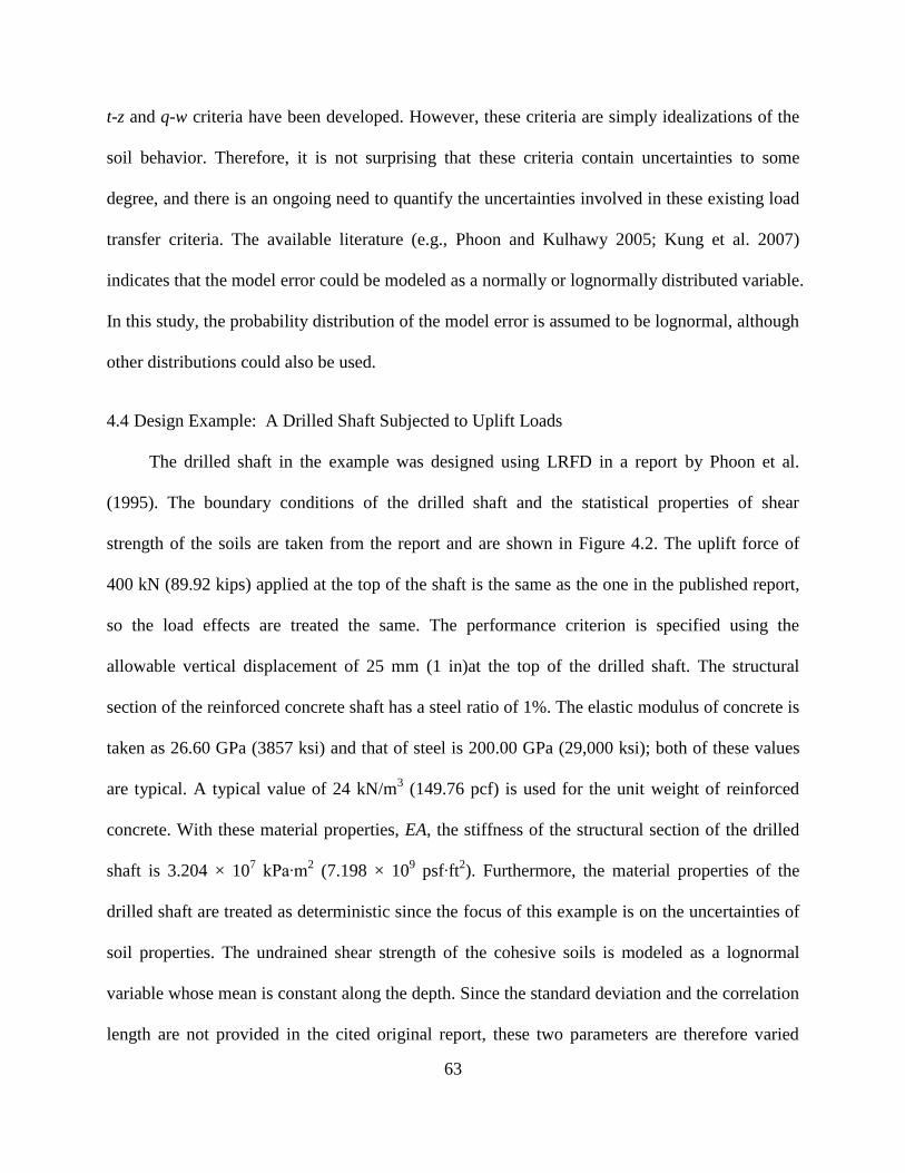
63
t-z and q-w criteria have been developed. However, these criteria are simply idealizations of the
soil behavior. Therefore, it is not surprising that these criteria contain uncertainties to some
degree, and there is an ongoing need to quantify the uncertainties involved in these existing load
transfer criteria. The available literature (e.g., Phoon and Kulhawy 2005; Kung et al. 2007)
indicates that the model error could be modeled as a normally or lognormally distributed variable.
In this study, the probability distribution of the model error is assumed to be lognormal, although
other distributions could also be used.
4.4 Design Example: A Drilled Shaft Subjected to Uplift Loads
The drilled shaft in the example was designed using LRFD in a report by Phoon et al.
(1995). The boundary conditions of the drilled shaft and the statistical properties of shear
strength of the soils are taken from the report and are shown in Figure 4.2. The uplift force of
400 kN (89.92 kips) applied at the top of the shaft is the same as the one in the published report,
so the load effects are treated the same. The performance criterion is specified using the
allowable vertical displacement of 25 mm (1 in)at the top of the drilled shaft. The structural
section of the reinforced concrete shaft has a steel ratio of 1%. The elastic modulus of concrete is
taken as 26.60 GPa (3857 ksi) and that of steel is 200.00 GPa (29,000 ksi); both of these values
are typical. A typical value of 24 kN/m3 (149.76 pcf) is used for the unit weight of reinforced
concrete. With these material properties, EA, the stiffness of the structural section of the drilled
shaft is 3.204 × 10⁷ kPa∙m
2 (7.198 × 10
9 psf∙ft
2). Furthermore, the material properties of the
drilled shaft are treated as deterministic since the focus of this example is on the uncertainties of
soil properties. The undrained shear strength of the cohesive soils is modeled as a lognormal
variable whose mean is constant along the depth. Since the standard deviation and the correlation
length are not provided in the cited original report, these two parameters are therefore varied
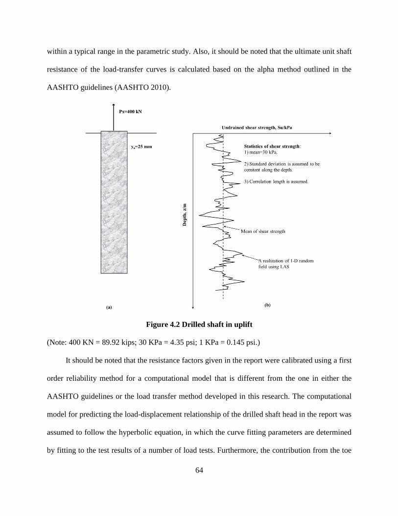
64
within a typical range in the parametric study. Also, it should be noted that the ultimate unit shaft
resistance of the load-transfer curves is calculated based on the alpha method outlined in the
AASHTO guidelines (AASHTO 2010).
Figure 4.2 Drilled shaft in uplift
(Note: 400 KN = 89.92 kips; 30 KPa = 4.35 psi; 1 KPa = 0.145 psi.)
It should be noted that the resistance factors given in the report were calibrated using a first
order reliability method for a computational model that is different from the one in either the
AASHTO guidelines or the load transfer method developed in this research. The computational
model for predicting the load-displacement relationship of the drilled shaft head in the report was
assumed to follow the hyperbolic equation, in which the curve fitting parameters are determined
by fitting to the test results of a number of load tests. Furthermore, the contribution from the toe
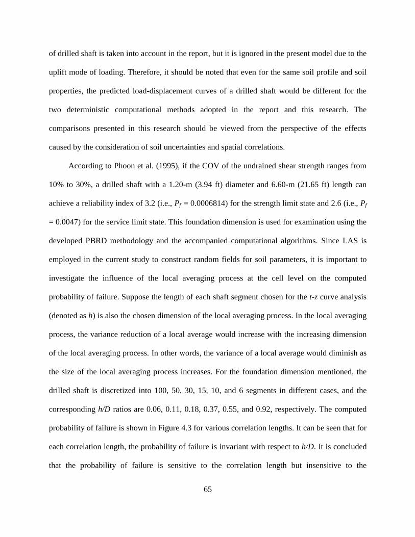
65
of drilled shaft is taken into account in the report, but it is ignored in the present model due to the
uplift mode of loading. Therefore, it should be noted that even for the same soil profile and soil
properties, the predicted load-displacement curves of a drilled shaft would be different for the
two deterministic computational methods adopted in the report and this research. The
comparisons presented in this research should be viewed from the perspective of the effects
caused by the consideration of soil uncertainties and spatial correlations.
According to Phoon et al. (1995), if the COV of the undrained shear strength ranges from
10% to 30%, a drilled shaft with a 1.20-m (3.94 ft) diameter and 6.60-m (21.65 ft) length can
achieve a reliability index of 3.2 (i.e., Pf = 0.0006814) for the strength limit state and 2.6 (i.e., Pf
= 0.0047) for the service limit state. This foundation dimension is used for examination using the
developed PBRD methodology and the accompanied computational algorithms. Since LAS is
employed in the current study to construct random fields for soil parameters, it is important to
investigate the influence of the local averaging process at the cell level on the computed
probability of failure. Suppose the length of each shaft segment chosen for the t-z curve analysis
(denoted as h) is also the chosen dimension of the local averaging process. In the local averaging
process, the variance reduction of a local average would increase with the increasing dimension
of the local averaging process. In other words, the variance of a local average would diminish as
the size of the local averaging process increases. For the foundation dimension mentioned, the
drilled shaft is discretized into 100, 50, 30, 15, 10, and 6 segments in different cases, and the
corresponding h/D ratios are 0.06, 0.11, 0.18, 0.37, 0.55, and 0.92, respectively. The computed
probability of failure is shown in Figure 4.3 for various correlation lengths. It can be seen that for
each correlation length, the probability of failure is invariant with respect to h/D. It is concluded
that the probability of failure is sensitive to the correlation length but insensitive to the

66
normalized cell size in LAS. Based on this parametric study, the number of increments used in
the design example is taken as 30. The adopted use of the shaft segment size in the discretization
process of the drilled shaft in the numerical algorithm would be acceptable, as it does not affect
the outcome of the computed probability of failure. Figure 4.4 shows examples of the computed
load-settlement curves using the developed computer program for a case with an assumed COV
of the shear strength of 30% and an assumed correlation length of 4.0 m (13.12 ft).
Figure 4.3 Relationship between Pf and the normalized size of local averaging process
(Note: 2 m = 6.56 ft; 4 m = 13.12 ft; 20 m = 65.62 ft.)
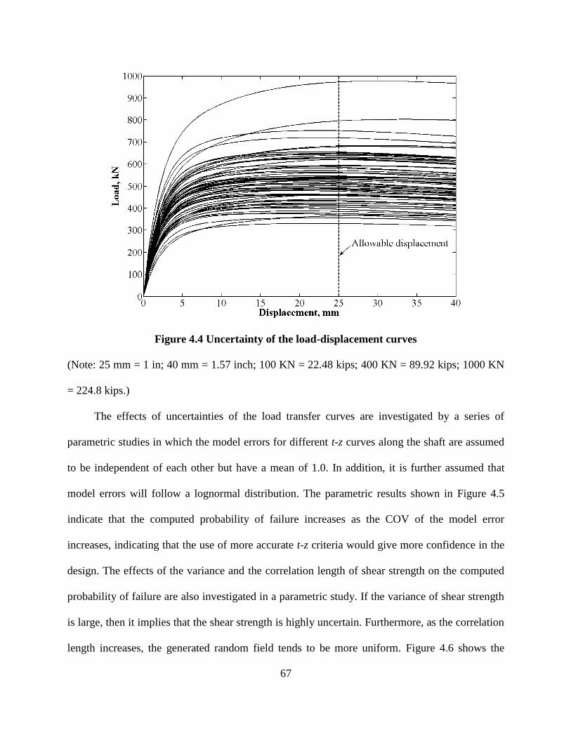
67
Figure 4.4 Uncertainty of the load-displacement curves
(Note: 25 mm = 1 in; 40 mm = 1.57 inch; 100 KN = 22.48 kips; 400 KN = 89.92 kips; 1000 KN
= 224.8 kips.)
The effects of uncertainties of the load transfer curves are investigated by a series of
parametric studies in which the model errors for different t-z curves along the shaft are assumed
to be independent of each other but have a mean of 1.0. In addition, it is further assumed that
model errors will follow a lognormal distribution. The parametric results shown in Figure 4.5
indicate that the computed probability of failure increases as the COV of the model error
increases, indicating that the use of more accurate t-z criteria would give more confidence in the
design. The effects of the variance and the correlation length of shear strength on the computed
probability of failure are also investigated in a parametric study. If the variance of shear strength
is large, then it implies that the shear strength is highly uncertain. Furthermore, as the correlation
length increases, the generated random field tends to be more uniform. Figure 4.6 shows the
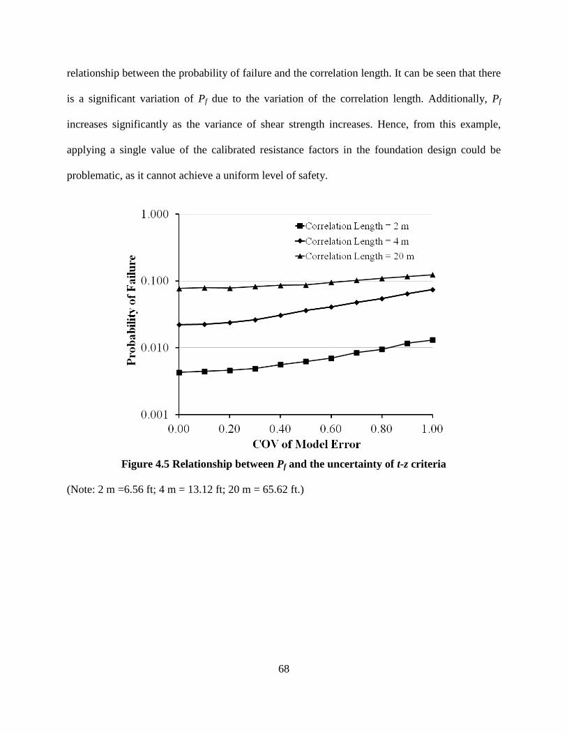
68
relationship between the probability of failure and the correlation length. It can be seen that there
is a significant variation of Pf due to the variation of the correlation length. Additionally, Pf
increases significantly as the variance of shear strength increases. Hence, from this example,
applying a single value of the calibrated resistance factors in the foundation design could be
problematic, as it cannot achieve a uniform level of safety.
Figure 4.5 Relationship between Pf and the uncertainty of t-z criteria
(Note: 2 m =6.56 ft; 4 m = 13.12 ft; 20 m = 65.62 ft.)
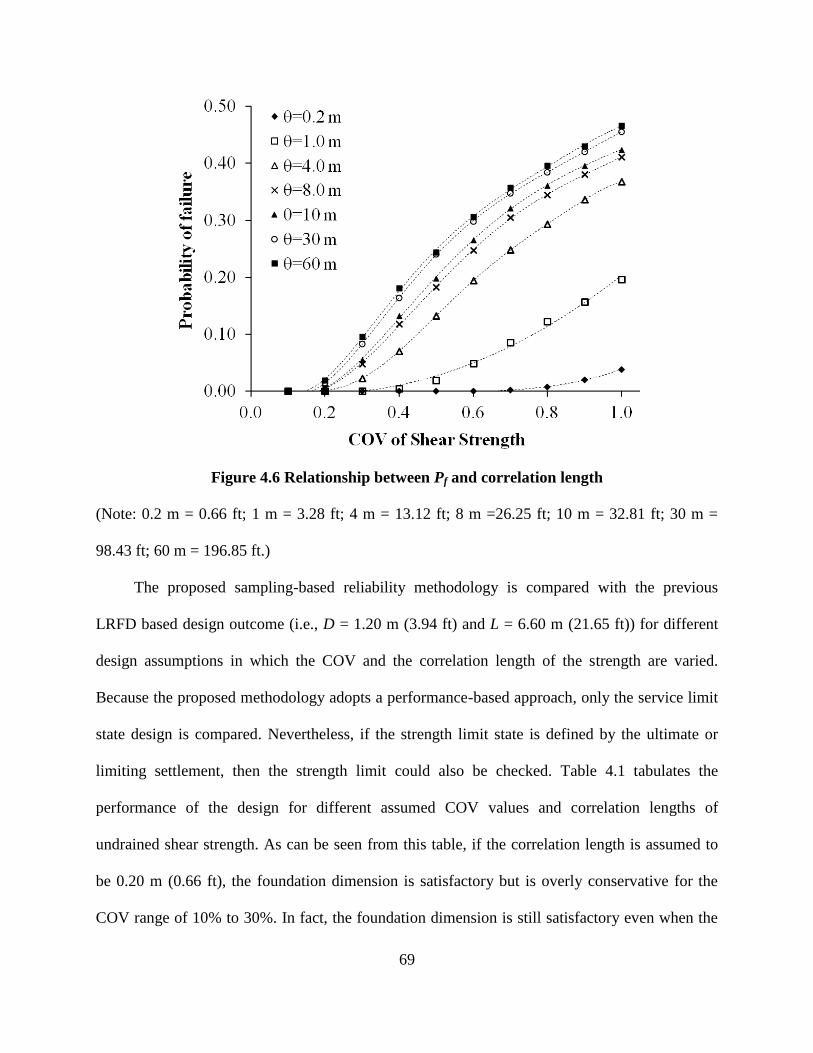
69
Figure 4.6 Relationship between Pf and correlation length
(Note: 0.2 m = 0.66 ft; 1 m = 3.28 ft; 4 m = 13.12 ft; 8 m =26.25 ft; 10 m = 32.81 ft; 30 m =
98.43 ft; 60 m = 196.85 ft.)
The proposed sampling-based reliability methodology is compared with the previous
LRFD based design outcome (i.e., D = 1.20 m (3.94 ft) and L = 6.60 m (21.65 ft)) for different
design assumptions in which the COV and the correlation length of the strength are varied.
Because the proposed methodology adopts a performance-based approach, only the service limit
state design is compared. Nevertheless, if the strength limit state is defined by the ultimate or
limiting settlement, then the strength limit could also be checked. Table 4.1 tabulates the
performance of the design for different assumed COV values and correlation lengths of
undrained shear strength. As can be seen from this table, if the correlation length is assumed to
be 0.20 m (0.66 ft), the foundation dimension is satisfactory but is overly conservative for the
COV range of 10% to 30%. In fact, the foundation dimension is still satisfactory even when the
70
COV of the shear strength is equal to 70%. However, if the correlation length is assumed to be
8.0 m (26.25 ft), the foundation dimension is satisfactory for a COV of 10% but unsatisfactory
for a COV of 20% or greater.
The performance of the aforementioned design outcome for two special cases (i.e., θ = 0
and θ = ∞) were also tabulated. If the correlation length is equal to zero, then the random field
becomes an infinite sequence of independent and identically distributed random variables. In this
case, the variance of a local average for any finite averaging dimension is equal to zero, which
means a random field based analysis become a deterministic analysis. For θ equal to 0, it can be
observed from Table 4.1 that the design outcome is satisfactory even when the COV of shear
strength is equal to 100%. At the other end of the scale, the correlation length is equal to infinity.
In this case, the random field is perfectly correlated, meaning that the random variables for a
stationary and perfectly correlated random field are identical. For θ equal to ∞, it can be
observed from Table 4.1 that the design outcome is satisfactory when the COV of shear strength
is equal to 10%, but it becomes unsatisfactory if the COV of shear strength is equal to or greater
than 20%. There may be a number of reasons for the observed differences between the design
outcomes given by these two approaches when various assumptions are made regarding the COV
and correlation length. First of all, the deterministic computational models for predicting the
load-displacement relationships are obviously different between these two approaches. In
addition, the correlation structures of soil parameters were not included in the calibration of
resistance factors in the report by Phoon et al. (1995).
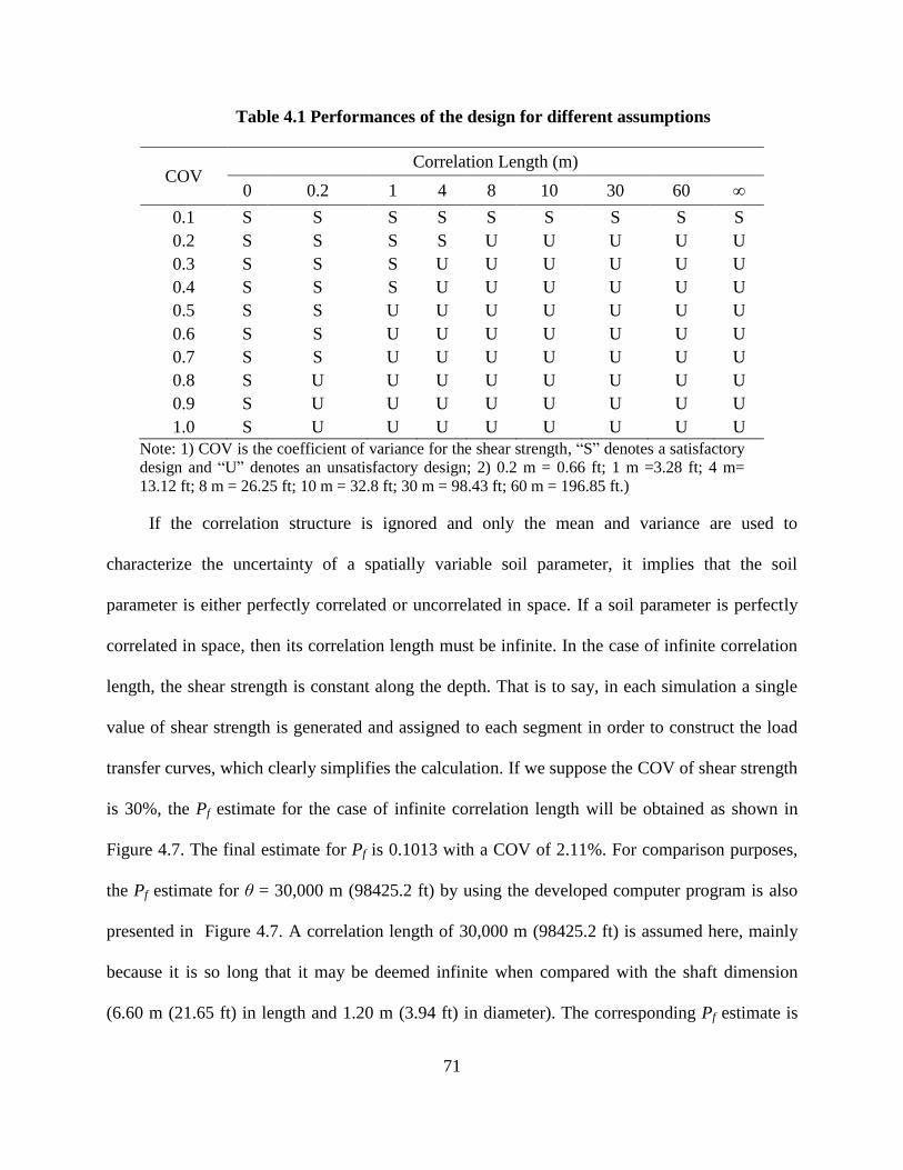
71
Table 4.1 Performances of the design for different assumptions
COV Correlation Length (m)
0 0.2 1 4 8 10 30 60 ∞
0.1 S S S S S S S S S
0.2 S S S S U U U U U
0.3 S S S U U U U U U
0.4 S S S U U U U U U
0.5 S S U U U U U U U
0.6 S S U U U U U U U
0.7 S S U U U U U U U
0.8 S U U U U U U U U
0.9 S U U U U U U U U
1.0 S U U U U U U U U
Note: 1) COV is the coefficient of variance for the shear strength, ―S‖ denotes a satisfactory
design and ―U‖ denotes an unsatisfactory design; 2) 0.2 m = 0.66 ft; 1 m =3.28 ft; 4 m=
13.12 ft; 8 m = 26.25 ft; 10 m = 32.8 ft; 30 m = 98.43 ft; 60 m = 196.85 ft.)
If the correlation structure is ignored and only the mean and variance are used to
characterize the uncertainty of a spatially variable soil parameter, it implies that the soil
parameter is either perfectly correlated or uncorrelated in space. If a soil parameter is perfectly
correlated in space, then its correlation length must be infinite. In the case of infinite correlation
length, the shear strength is constant along the depth. That is to say, in each simulation a single
value of shear strength is generated and assigned to each segment in order to construct the load
transfer curves, which clearly simplifies the calculation. If we suppose the COV of shear strength
is 30%, the Pf estimate for the case of infinite correlation length will be obtained as shown in
Figure 4.7. The final estimate for Pf is 0.1013 with a COV of 2.11%. For comparison purposes,
the Pf estimate for θ = 30,000 m (98425.2 ft) by using the developed computer program is also
presented in Figure 4.7. A correlation length of 30,000 m (98425.2 ft) is assumed here, mainly
because it is so long that it may be deemed infinite when compared with the shaft dimension
(6.60 m (21.65 ft) in length and 1.20 m (3.94 ft) in diameter). The corresponding Pf estimate is

72
0.1015 with a COV of 2.10%. It is clear that the results obtained by the two simulation
approaches agree very well.
Figure 4.7 Convergence of Pf estimates based on simplified MCS and P-TZPILE
(Note: 30,000 m = 98425.2 ft.)
In contrast, if the soil parameter is uncorrelated in space, then the correlation length has to
be equal to zero. Again suppose that the COV of shear strength is 30% for a lognormal variable
with zero correlation length; its median of 28.73 kPa (4.16 psi) is assigned to each segment as
the shear strength. A deterministic analysis was conducted and the uplift capacity was
determined to be 499.0093 kN (112.18 kips) based on the allowable displacement. For
comparison purposes, a random field–based analysis was conducted for this case with a θ equal
to 1.0 × 10⁻⁷
m (3.28 × 10⁻⁷
ft). Correlation length of 1.0 × 10⁻⁷
m (3.28 × 10⁻⁷
ft) is assumed here,
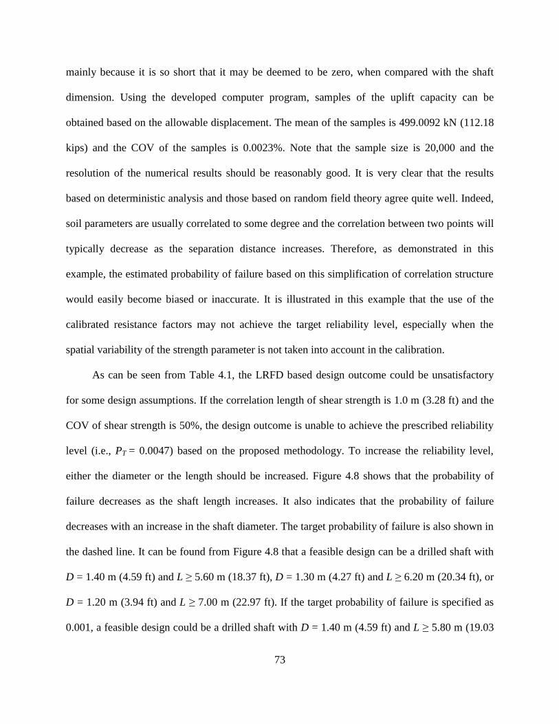
73
mainly because it is so short that it may be deemed to be zero, when compared with the shaft
dimension. Using the developed computer program, samples of the uplift capacity can be
obtained based on the allowable displacement. The mean of the samples is 499.0092 kN (112.18
kips) and the COV of the samples is 0.0023%. Note that the sample size is 20,000 and the
resolution of the numerical results should be reasonably good. It is very clear that the results
based on deterministic analysis and those based on random field theory agree quite well. Indeed,
soil parameters are usually correlated to some degree and the correlation between two points will
typically decrease as the separation distance increases. Therefore, as demonstrated in this
example, the estimated probability of failure based on this simplification of correlation structure
would easily become biased or inaccurate. It is illustrated in this example that the use of the
calibrated resistance factors may not achieve the target reliability level, especially when the
spatial variability of the strength parameter is not taken into account in the calibration.
As can be seen from Table 4.1, the LRFD based design outcome could be unsatisfactory
for some design assumptions. If the correlation length of shear strength is 1.0 m (3.28 ft) and the
COV of shear strength is 50%, the design outcome is unable to achieve the prescribed reliability
level (i.e., PT = 0.0047) based on the proposed methodology. To increase the reliability level,
either the diameter or the length should be increased. Figure 4.8 shows that the probability of
failure decreases as the shaft length increases. It also indicates that the probability of failure
decreases with an increase in the shaft diameter. The target probability of failure is also shown in
the dashed line. It can be found from Figure 4.8 that a feasible design can be a drilled shaft with
D = 1.40 m (4.59 ft) and L ≥ 5.60 m (18.37 ft), D = 1.30 m (4.27 ft) and L ≥ 6.20 m (20.34 ft), or
D = 1.20 m (3.94 ft) and L ≥ 7.00 m (22.97 ft). If the target probability of failure is specified as
0.001, a feasible design could be a drilled shaft with D = 1.40 m (4.59 ft) and L ≥ 5.80 m (19.03

74
ft), D = 1.30 m (4.27 ft) and L ≥ 6.60 m (21.65 ft), or D = 1.20 m (3.94 ft) and L ≥ 7.20 m (23.62
ft). Likewise, the feasible designs for other prescribed reliability levels can be found
conveniently from this figure. Among the feasible designs, one can find the optimal design with
consideration of the economic constraints (e.g., Wang et al. 2011).
Figure 4.8 Probabilities of failure for different designs
(Note: 1.2 m = 3.94 ft; 1.3 m 4.27 ft; 1.4 m = 4.59 ft; 5 m =16.4 ft; 6 m= 19.68 ft; 7 m = 22.97 ft;
8 m = 26.25 ft.)
4.5 Design Example: A Drilled Shaft Subjected to Compression
Consider the example drilled shaft shown in Figure 4.9. The compressive force applied at
the top of the shaft is 600 kN (134.88 kips) and is assumed to be deterministic. The limiting
vertical displacement is assumed to be 25 mm (1 in). Failure is said to occur if the shaft head

75
displacement exceeds 25 mm (1 in). The section of the reinforced concrete shaft has a steel ratio
of 1%. The compressive strength of concrete is given as 31027.5 kPa (4.5 ksi), and a typical
value of 200 GPa (29,000 ksi) is used for the elastic modulus of steel. A typical value of 24
kN/m3 (149.76 pcf) is used for the unit weight of reinforced concrete and is assumed to be
deterministic. The undrained shear strength of cohesive soils is modeled as a lognormal variable
with a standard deviation of 30 kPa (4.35 psi). The mean of the shear strength is constant at the
top three meters and then increases linearly with depth (see Figure 4.9). Indeed, it is not unusual
for the soil properties to vary with depth. The shear strength of clay along the depth is modeled
as one-dimensional (1-D) random fields, which are generated using LAS. The aforementioned
values are used as inputs in the developed computer program. The alpha method outlined in
AASHTO (2010) is used to calculate the ultimate load transfer of the load-transfer curves. For
illustration purposes, the normalized load-transfer curves shown in Figure 2.3 are assumed to be
certain, and they are employed to predict the load-settlement curves.
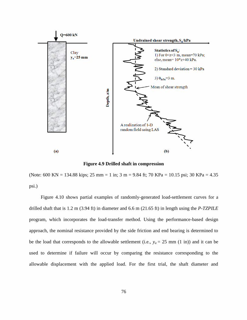
76
Figure 4.9 Drilled shaft in compression
(Note: 600 KN = 134.88 kips; 25 mm = 1 in; 3 m = 9.84 ft; 70 KPa = 10.15 psi; 30 KPa = 4.35
psi.)
Figure 4.10 shows partial examples of randomly-generated load-settlement curves for a
drilled shaft that is 1.2 m (3.94 ft) in diameter and 6.6 m (21.65 ft) in length using the P-TZPILE
program, which incorporates the load-transfer method. Using the performance-based design
approach, the nominal resistance provided by the side friction and end bearing is determined to
be the load that corresponds to the allowable settlement (i.e., ya = 25 mm (1 in)) and it can be
used to determine if failure will occur by comparing the resistance corresponding to the
allowable displacement with the applied load. For the first trial, the shaft diameter and
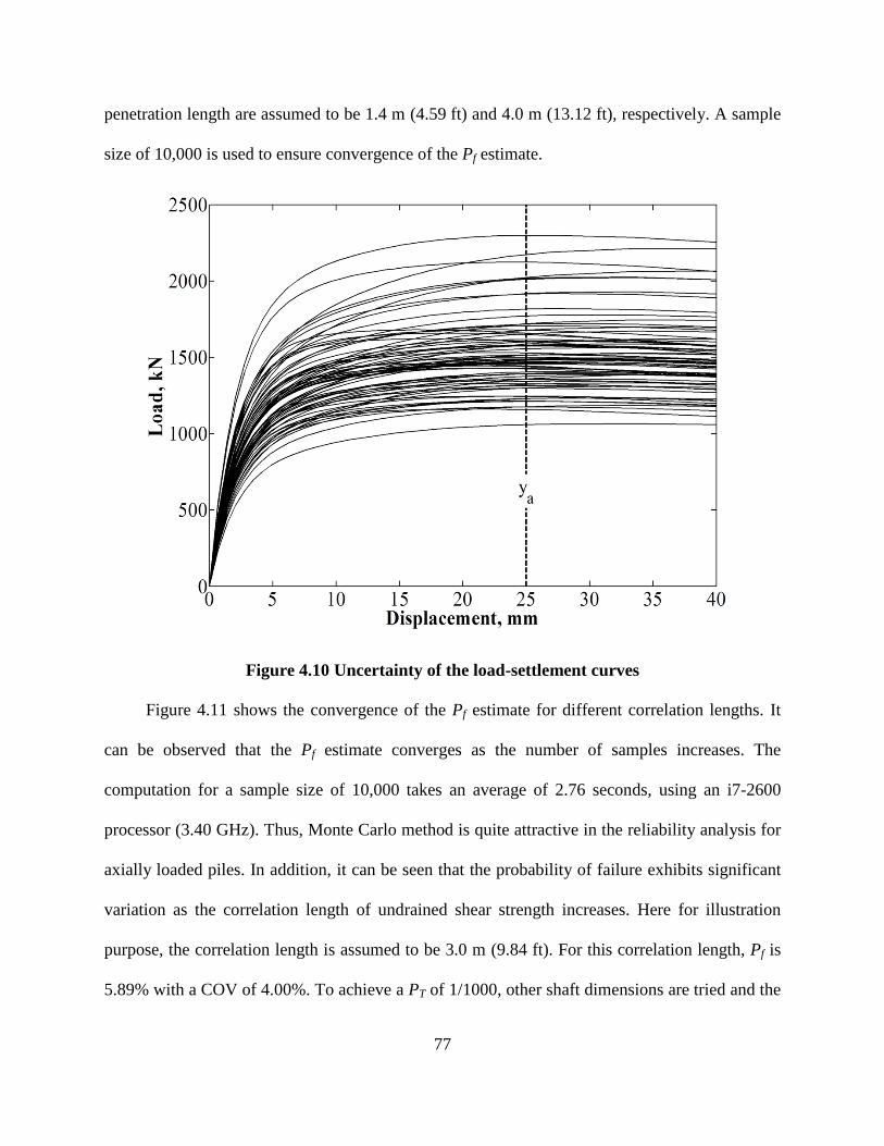
77
penetration length are assumed to be 1.4 m (4.59 ft) and 4.0 m (13.12 ft), respectively. A sample
size of 10,000 is used to ensure convergence of the Pf estimate.
Figure 4.10 Uncertainty of the load-settlement curves
Figure 4.11 shows the convergence of the Pf estimate for different correlation lengths. It
can be observed that the Pf estimate converges as the number of samples increases. The
computation for a sample size of 10,000 takes an average of 2.76 seconds, using an i7-2600
processor (3.40 GHz). Thus, Monte Carlo method is quite attractive in the reliability analysis for
axially loaded piles. In addition, it can be seen that the probability of failure exhibits significant
variation as the correlation length of undrained shear strength increases. Here for illustration
purpose, the correlation length is assumed to be 3.0 m (9.84 ft). For this correlation length, Pf is
5.89% with a COV of 4.00%. To achieve a PT of 1/1000, other shaft dimensions are tried and the

78
results are summarized in Table 4.2. From the tabulated results, it can be seen that drilled shafts
with D = 1.20 m (3.94 ft) and L ≥ 6.00 m (19.68 ft), or D = 1.40 m (4.59 ft) and L ≥ 5.40 m
(17.72 ft) would meet the specified performance criteria. It is noted that other feasible designs
(i.e., combinations of D and L) should be checked as well for choosing final optimal design.
Figure 4.11 Convergence of Pf estimates by MCS
(Note: 1 m = 3.28 ft; 3 m = 9.84 ft; 5 m = 16.40 ft; 10 m = 32.81 ft; 40 m = 131.23 ft.)

79
Table 4.2 Probabilities of Failure obtained by MCS
L (m) D = 1.2 m D = 1.4 m
Pf n COV(Pf) Pf n COV(Pf)
4.0 1.64E-01 10000 2.26% 5.89E-02 10000 4.00%
4.2 1.24E-01 10000 2.65% 4.12E-02 10000 4.82%
4.4 9.05E-02 10000 3.17% 2.45E-02 10000 6.31%
4.6 6.45E-02 10000 3.81% 1.49E-02 10000 8.13%
4.8 4.20E-02 10000 4.78% 7.60E-03 10000 11.43%
5.0 2.42E-02 10000 6.35% 3.00E-03 10000 18.23%
5.2 1.64E-02 10000 7.74% 1.50E-03 10000 25.80%
5.4 7.20E-03 10000 11.74% 5.67E-04 30000 24.25%
5.6 3.60E-03 10000 16.64% 3.67E-04 30000 30.15%
5.8 1.90E-03 20000 16.21% 3.33E-05 30000 100.00%
6.0 5.50E-04 20000 30.14% 3.33E-05 30000 100.00%
Note: 1) n is the sample size for MCS; 2) COV(Pf) is the coefficient of variation for Pf; 3) 1.2 m =
3.94 ft; 1.4 m = 4.59 ft; 4 m = 13.12 ft; 5 m = 16.40 ft; 6 m = 19.69 ft.
4.6 Summary and Conclusions
A performance-based design computational method based on Monte Carlo statistical
methods was presented in this chapter for the analysis and design of a drilled shaft subjected to
axial loads. In the proposed framework, the uncertainties arising from the input (e.g., the
undrained shear strength for cohesive soils) for the computational model and the model error (i.e.,
the error of t-z and q-w criteria) were treated as random variables. In particular, the spatial
variance of soil properties is explicitly accounted for by using random field modeling. The local
averaging subdivision technique was used to generate a large number of random samples
according to the statistical descriptors including mean, variance, probability distribution function,
and correlation length. The generated samples are used as input to evaluate the axial
displacement of the drilled shaft under the applied axial loads. The probability of failure
determined on the basis of the specified performance criteria (i.e., the allowable drilled shaft
head movement) can be computed accordingly. The performance-based design involves

80
adjusting the design parameters (i.e., the diameter and length of the drilled shaft) until the
calculated probability of failure is equal to or smaller than the target probability of failure. A
computer program called P-TZPILE, which uses the traditional load transfer concepts involving
nonlinear t-z and q-w curves, was developed to implement the proposed methodology for the
reliability analysis of an axially loaded drilled shaft.
Two design examples were presented in this chapter to illustrate the application of the
developed method. The examples demonstrated that the probabilistic approaches that do not take
into consideration the spatial variance of soil properties may potentially result in a foundation
design that would not meet the performance criteria with the target reliability. There is a strong
incentive to use a reliability-based method that considers the correlation structure of soil
properties for deep foundations.
81
CHAPTER 5. ANALYSIS OF SYSTEM RELIABILITY
5.1 Introduction
In the LRFD approach LRFD, different limit states are considered separately and no
system reliability is taken into account. Therefore, it is desirable to develop a probabilistic
approach to tackle the uncertainties in the reliability-based design to address those issues
described earlier. In this chapter, the serviceability performance of drilled shafts under combined
lateral and axial loading is investigated using reliability analysis. Note that the terms ―pile‖ and
―drilled shaft‖ will be used interchangeably in this report.
Drilled shafts are widely used to resist axial and lateral loads. Under the loading, a drilled
shaft typically has three distinctive displacements: lateral deflection (δ), angular distortion (ψ),
and axial movement (w) at the top of the shaft. The performance of the pile is defined in terms of
these displacements. To conduct reliability analysis for each limit state and assess the system
reliability, Monte Carlo simulation (MCS) is applied. Since there are various sources of
uncertainties involved in the reliability analysis, importance analysis is conducted in order to
identify the sources of uncertainties that will significantly affect the serviceability performance.
5.2 Reliability Assessment
The failure (or unsatisfactory performance) event in this study is said to occur if the
induced displacements at the top of the pile are greater than the corresponding allowable
displacements. System failure in this study is defined as the event in which any of the individual

82
failure modes occurs. Following the conventional notation in structural reliability theory
(Ditlevsen and Madsen 1996), probability of system failure, Pf, can be expressed by
, 0f k k k
k
P P g C D
x
(5.1)
where the subscript k represents a serviceability failure mode (i.e., k = δ, ψ and w), gk(·) refers to
the k-th limit state function, Ck represents the allowable displacement, Dk is the induced
displacement due to the external loads, and x = (xr, xd) refer to the input variables (e.g., geometry
and material properties) in which xr are random variables and xd are deterministic variables. In
this study, the limit state function for the k-th failure mode is defined as
k k kg C D x (5.2)
Using the probability of failure for the k-th limit state (Pf,k), the corresponding reliability index,
βk, can be determined by
1 1
, ,1k f k f kP P (5.3)
where Φ-1
(∙) is the inverse of the cumulative distribution function of the standard normal
variable.
In this study, the induced displacement Dk is obtained through the analysis of drilled shafts
subjected to axial and lateral loading where the load transfer methods—for example, the t-z
model proposed by Coyle and Reese (1966) and the p-y method proposed by Reese (1977)—are
applied to model the nonlinear soil-pile interactions. The t-z model can be used to calculate the
vertical movement where the axial soil-pile interaction is modeled as t-z curves and q-w curves,
in which t and q represent side shear on the shaft and the tip resistance at the toe, respectively,
and z and w represent the vertical displacements of the shaft segment and the toe of the drilled
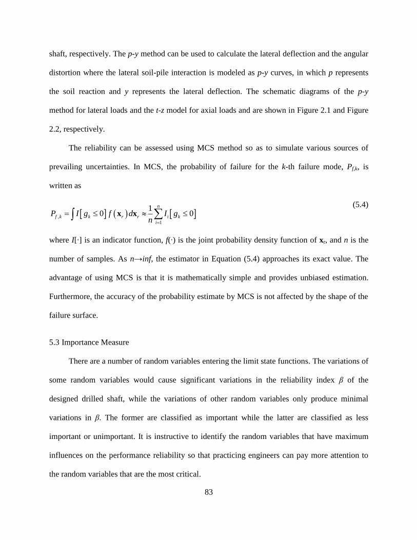
83
shaft, respectively. The p-y method can be used to calculate the lateral deflection and the angular
distortion where the lateral soil-pile interaction is modeled as p-y curves, in which p represents
the soil reaction and y represents the lateral deflection. The schematic diagrams of the p-y
method for lateral loads and the t-z model for axial loads and are shown in Figure 2.1 and Figure
2.2, respectively.
The reliability can be assessed using MCS method so as to simulate various sources of
prevailing uncertainties. In MCS, the probability of failure for the k-th failure mode, Pf,k, is
written as
,
1
10 0
n
f k k r r i k
i
P I g f d I gn
x x (5.4)
where I[∙] is an indicator function, f(∙) is the joint probability density function of xr, and n is the
number of samples. As n→inf, the estimator in Equation (5.4) approaches its exact value. The
advantage of using MCS is that it is mathematically simple and provides unbiased estimation.
Furthermore, the accuracy of the probability estimate by MCS is not affected by the shape of the
failure surface.
5.3 Importance Measure
There are a number of random variables entering the limit state functions. The variations of
some random variables would cause significant variations in the reliability index β of the
designed drilled shaft, while the variations of other random variables only produce minimal
variations in β. The former are classified as important while the latter are classified as less
important or unimportant. It is instructive to identify the random variables that have maximum
influences on the performance reliability so that practicing engineers can pay more attention to
the random variables that are the most critical.

84
The importance measure can be used to identify the importance of random variables.
According to Der Kiureghian and Ke (1995), an importance measure κ is defined as follows
*, *
*, *
T
u xT
T
u x
α J B
α J B
(5.5a)
G
G
u
u (5.5b)
*, * *, *
T
x u x uΣ J J (5.5c)
where G(u) = g(x(u)), ∇G(u)is the gradient vector evaluated at the design point xr* in the
standard normal space u, Ju*,x* is the Jacobian matrix of the probability transformation from the
original space xr to the standard normal space u with respect to the design point and is equal to
the inverse of Jx*,u*, the superscript ―T‖ denotes transpose, B is a diagonal matrix consisting of
the standard deviations of equivalent normal variables x′r that can be calculated with respect to
the design point, ∑ is the covariance matrix of xr. If a random variable is not normally
distributed, it has to be transformed to an equivalent normal variable according to its distribution
type, mean, and variance.
5.4 Random Variables
In this study, there are a number of sources of uncertainty. These sources include soil
variability; the variability of concrete and reinforcement material properties; the model errors in
p-y curves, t-z curves, and q-w curves; the uncertainty in the performance criteria; and the load
variability. These uncertainties are considered through the random variables xr. This section
describes the probabilistic modeling of these random variables.

85
It should be noted that the performance of the designed drilled shafts is clearly affected by
construction. Even if the design is appropriate, the actual performance may be unsatisfactory
when the construction quality is poor. Therefore, the construction-related uncertainty should be
treated as a factor that is as important as the aforementioned uncertainties. However, it is
difficult to quantify construction-related uncertainty because the construction process is complex
and has many implications. For example, the construction process may directly affect the
surrounding soils and the strength of the concrete. As the complexity of these implications is
beyond the research scope of this research, it is assumed that the drilled shafts in this study are
properly constructed such that the influence of the construction-related uncertainty can be
ignored.
5.4.1 Soil Properties
The analysis of a pile subjected to axial load and lateral load is a complex problem in
which the soil-structure interaction is involved. In the analysis, the uncertainty of soil properties
propagates through the p-y curves, t-z curves, and q-w curves used in the soil-structure
interaction analysis. Cohesive soils can be used as an example. Soil properties are needed for
constructing t-z curves, q-w curves, and p-y curves; these soil properties include undrained shear
strength Su, effective unit weight γ', and ε50 (where ε50 is defined as 50% of the strain
corresponding to the maximum principal stress difference). . Soil itself is a complicated material
in which physical process and chemical process are involved, resulting in relatively large
variability in the soil properties. In addition, statistical uncertainty and transformation error are
introduced in the sampling process and the testing process (e.g., Phoon and Kulhawy 1999).
Thus, an appropriate soil variability model is needed in the reliability analysis. To capture the
spatial correlation, each soil property (Su, γ', and ε50) is modeled as a random field that is

86
statistically characterized by three parameters: the mean μ, variance ζ2 and correlation length θ.
The mean measures the center of a dataset and the variance measures the dispersion from the
center, while the correlation length measures how rapidly a random field varies in space. The
way in which a random field varies depends on its correlation structure, which is considered
through a correlation function.
5.4.2 Material Properties
The materials for constructing drilled shafts include concrete and steel reinforcing bars (or
rebar). The strength of concrete inevitably has some degree of variation. According to the
American Concrete Institute (2002), the coefficient of variation (COV) for concrete compressive
strength, f′c, is generally in the range of 3% to 10%, depending on the concrete production and
transportation process, the sampling process, and the testing process. The mechanical properties
of reinforcement also have some degree of variation. It is known that a number of factors,
including the rate of loading and the cross-sectional area of the rebars, can directly affect the
yield strength of rebars. According to Mirza and MacGregor (1979), the COV for the yield
strength of rebars, fy, is typically in the range of 1% to 12%.
5.4.3 Model Errors
Model uncertainty is always present, as any computational model is an idealization or
simplification of real-world conditions. Suppose Ym denotes the prediction based on a model it
assumes to be unbiased, and em is a model factor for capturing the model error that leads to
potential under- or over- estimates. Thus, the true behavior (denoted as Yt) can be expressed as
follows:
t m mY e Y (5.6)
87
It should be noted that the error term em should be considered as a random variable whose
statistical characters can be described using lognormal distributions (e.g., Phoon and Kulhawy
2005).
The accuracy of the p-y method (for calculating lateral deflection and angular distortion)
and the t-z model (for calculating vertical movement) is primarily affected by the modeling of
soil-pile interactions, which are represented by the p-y curves, t-z curves, and q-w curves.
However, the development of these curves is usually based on limited load tests, and the curves
may not truly represent the reality in which soils can vary significantly from one site to another.
Furthermore, various errors are involved in the load test data. For example, there are
measurement errors in the strain gauges used for estimating the axial deformations and
curvatures induced by bending moment. Therefore, the model error in the p-y curves, t-z curves,
and q-w curves needs to be considered for the soil-pile interaction analysis.
5.4.4 Allowable Displacements
The design of drilled shafts must satisfy strength and serviceability performance
requirements. The serviceability check requires that the displacement induced by external loads
should not be greater than the maximum allowable displacement. Maximum allowable
displacements are traditionally treated as deterministic.
However, the specified allowable displacement is uncertain to some extent. The allowable
displacement is primarily determined by the superstructure under consideration through
structural analysis. The outcome of the structural analysis is dependent on the models employed
and the corresponding input (i.e., material and geometry properties). Therefore, the outcome of
interest (i.e., the allowable displacements in this study) has some variations due to the
uncertainties in the models and the inputs used in the structural analysis.

88
5.4.5 External Loads
The variability in the design loads applied to the pile foundations should be considered, as
the external loads can directly affect the displacement of a designed structure. According to
Nowak and Collins (2000), the COV for dead load could range from 0.08 to 0.10 for buildings
and bridges, while those for live load (including sustained live load and transient live load) could
range from 0.18 to 0.89. Previous investigations (e.g., Ellingwood and Tekie 1999; Ellingwood
et al. 1980) have found that normal, lognormal, gamma, Type-I and Type-II Gumbel
distributions are possible choices to statistically characterize load models. For example, the
maximum live load for a structure can be statistically characterized by Type-I Gumbel
distributions, while sustained live load can be modeled as a gamma-distributed random variable.
5.5 Example
This section presents an example of reliability-based assessment for a drilled shaft and the
importance analysis of the random variables that are considered in the reliability analysis. The
configuration of the example of a drilled shaft is shown in Figure 5.1. It is assumed that the pile
is constructed in a stiff clay site. The drilled shaft is 1.0 m (3.28 ft) in diameter and 8.0 m (26.25
ft) in length. The cross-section of the shaft is reinforced by a total of 12 No. 11 rebars (with a
nominal diameter equal to 3.581 cm (1.41 in)), a reinforcement ratio of 1%, and a cover
thickness of 7.62 cm (3 in).
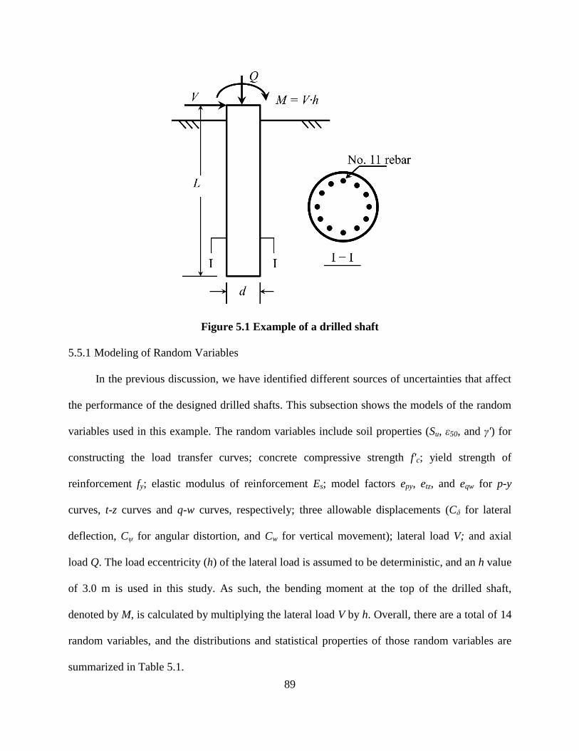
89
Figure 5.1 Example of a drilled shaft
5.5.1 Modeling of Random Variables
In the previous discussion, we have identified different sources of uncertainties that affect
the performance of the designed drilled shafts. This subsection shows the models of the random
variables used in this example. The random variables include soil properties (Su, ε50, and γ') for
constructing the load transfer curves; concrete compressive strength f'c; yield strength of
reinforcement fy; elastic modulus of reinforcement Es; model factors epy, etz, and eqw for p-y
curves, t-z curves and q-w curves, respectively; three allowable displacements (Cδ for lateral
deflection, Cψ for angular distortion, and Cw for vertical movement); lateral load V; and axial
load Q. The load eccentricity (h) of the lateral load is assumed to be deterministic, and an h value
of 3.0 m is used in this study. As such, the bending moment at the top of the drilled shaft,
denoted by M, is calculated by multiplying the lateral load V by h. Overall, there are a total of 14
random variables, and the distributions and statistical properties of those random variables are
summarized in Table 5.1.

90
Table 5.1 Statistical properties of random variables.
Variable Distribution Mean COV
Su Lognormal 120 KPa 50%
ε50 Lognormal 0.002 15%
γ' Lognormal 19 KN/m3 3%
f'c Gumbel 32 MPa 7%
fy Gumbel 415 MPa 5%
Es Lognormal 200 GPa 5%
epy Lognormal 1.0 5%
etz Lognormal 1.0 5%
eqw Lognormal 1.0 5%
Cδ Gumbel 2.0 cm 10%
Cψ Gumbel 0.01 10%
Cw Gumbel 2.5 cm 10%
V Gamma 200 KN 15%
Q Gamma 1000 KN 10%
(Note: 120 KPa = 17.4 psi; 19 KN/m3 = 118.56 pcf; 32 MPa = 4640 psi; 415 MPa = 60.18 ksi;
200 GPa = 29000 ksi; 2 cm = 0.79 in; 2.5 cm = 1 in; 200 KN = 44.96 kips; 1000 KN = 224.8
kips.)
It is noted that the mean values and the COVs listed in Table 5.1 are typical for the random
variables of interest except for those of ε50 and the model factors (epy, etz, and eqw). To the best
knowledge of the authors, the statistical properties of the model factors for the load transfer
curves and ε50 are not widely available in the literature. In this example, the mean values of the
model factors are assumed to be 1.0, implying that they are not under- or over-estimated in
predicting soil reactions, and the COVs of the model factors are assumed to be 5%. The mean of
ε50 for stiff clay is assumed to be 0.005 (the default value when test data is unavailable), and the
COV of ε50 is taken as 15%. The typical variability levels for the remaining random variables can
be readily found in the literature (e.g., Zhang and Ng 2005; Phoon and Kulhawy 2005; Nowak
and Collins 2000; Ellingwood et al. 1980).

91
To simulate the lateral soil-pile interaction, the p-y curve for stiff clay without free water is
used (Reese et al. 2004). The t-z curves and the q-w curves in this example are adopted from
AASHTO (2010) to represent the axial soil reaction for cohesive soils. Three soil properties
(namely Su, γ' and ε50) are used to construct the load transfer curves. As mentioned earlier, soil
properties are modeled as random fields in which the correlation lengths are needed to
characterize the dependence structure. In this example, the correlation lengths for Su, γ' and ε50
are taken as 1.0 m.
5.5.2 Reliability Analysis
Once the statistical properties of the random variables are defined, MCS is employed to
conduct reliability analysis. In MCS, the soil properties are simulated using the local averaging
subdivision (LAS) technique (Fenton and Griffiths 2008), which has proven to be a fast and
accurate method of producing random fields. In each realization, the displacements (δ, ψ and w)
at the top of the pile are evaluated repeatedly using a different set of soil properties as inputs to
the t-z model and the p-y method. With the resulting realizations of the displacements and the
realizations of the allowable displacements, the failure probabilities for each limit state and the
system can be evaluated accordingly.
Figure 5.2 shows the estimates of the failure probabilities for lateral deflection (Pf,δ),
angular distortion (Pf,ψ), vertical movement (Pf,w), and system failure (Pf). As expected, the
failure probabilities converge as the number of samples increases. As shown in Figure 5.2, the
failure probability of the system Pf is greater than that for any of the three individual failure
modes and is less than the summation of the failure probabilities of the individual failure modes.
The system failure probability will be underestimated if multiple failure modes are not
considered simultaneously, while the system failure probability will be overestimated as different
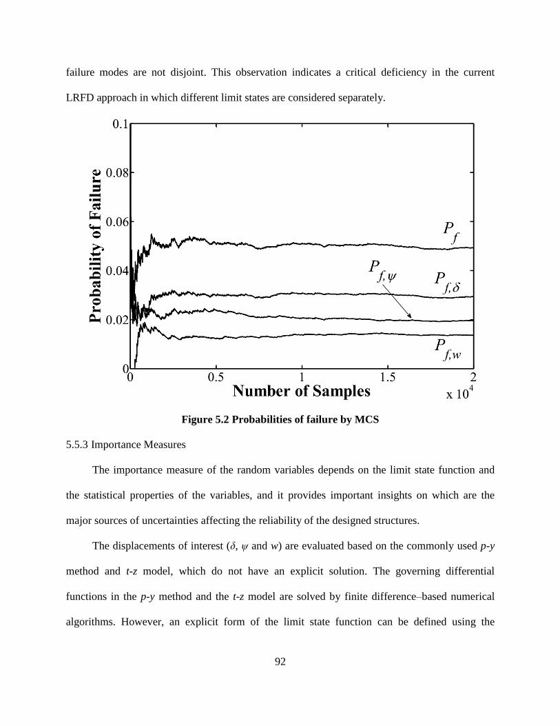
92
failure modes are not disjoint. This observation indicates a critical deficiency in the current
LRFD approach in which different limit states are considered separately.
Figure 5.2 Probabilities of failure by MCS
5.5.3 Importance Measures
The importance measure of the random variables depends on the limit state function and
the statistical properties of the variables, and it provides important insights on which are the
major sources of uncertainties affecting the reliability of the designed structures.
The displacements of interest (δ, ψ and w) are evaluated based on the commonly used p-y
method and t-z model, which do not have an explicit solution. The governing differential
functions in the p-y method and the t-z model are solved by finite difference–based numerical
algorithms. However, an explicit form of the limit state function can be defined using the

93
response surface method. A quadratic form of the limit state function is adopted in this study and
is defined as follows:
2
, ,
1 1
m m
r i r i i r i
i i
G c a x b x
x (5.7)
where ai, bi and c are regression coefficients, and xr = (xr,1, xr,2, …, xr,m) are the random variables.
The regression coefficients are determined using the method of least squares. It should be
pointed out that other forms of the limit state function may be applicable. For example, the
interaction terms between different random variables (such as xr,i∙xr,j) may be included. The
advantage of using a quadratic limit state function is that it becomes straightforward and efficient
to evaluate the gradient of the function that is needed in the importance analysis.
Figure 5.3 shows the importance measures for the three failure modes. For lateral
deflection (k = δ) and angular distortion (k = ψ) failure modes, the most important variables are
lateral load (V) and their corresponding allowable displacements. In contrast to the other two
modes, the vertical movement failure mode (k = w) has Su as the most important variable and Q
as the second most important variable.
Although the COVs of V and Q are just 15% and 10%, respectively, the external loads
overall still outweigh other random variables. This is understandable, since the lateral deflection
and the angular distortion are the direct response of V, and the vertical movement is the direction
response of Q. Furthermore, the allowable displacements are important, because they directly
reflect the ―capacity‖ in the limit state functions.

94
Figure 5.3 Importance measures of random variables

95
It should be noted that Su is a measure of soil strength, and it is assumed to have a large
variability (i.e., its COV is assumed to be as much as 50% in this example). Surprisingly, the
variability of Su is relatively less important for k = δ and k = ψ, but it is the most important
variable for k = w. On the other hand, even though the COVs for the model factors (epy, etz, eqw)
are just 5%, the importance measure of epy is large for both k = δ and k = ψ, and the importance
measures of etz and eqw are large for k = w. This observation indicates that the accuracy of the
load transfer curves is important in the reliability analyses. Moreover, f′c, fy, ε50 and γ', can be
considered unimportant random variables for all three failure modes.
Based on the evaluation of importance measures, it is concluded that the major sources of
uncertainties affecting the reliability of a designed drilled shaft come from the external loads, the
allowable displacements, the variability of Su, and the accuracy of the load transfer curves.
5.5.4 Influence of External Loads
In order to further investigate how the random variables affect the responses of the pile
system, an importance analysis is conducted given certain values of the external loading. Figures
5.4 and 5.5 show the importance measures in which Q is kept equal to 1000 KN (224.8 kips) and
V is varied, while Figure 5.6 shows the importance measures in which V is kept equal to 200 KN
(44.96 kips) and Q is varied. Only the first four most important random variables are shown in
these figures. Furthermore, it can be noticed that the change in V (168 KN (37.77 kips) to 270
KN (60.70 kips)) in Figures 5.4 and 5.5 leads to the changes in the reliability indices (βδ ranges
from 0.53 to 5.35, while βψ ranges from 0.70 to 5.50). Likewise, the change in Q (700 KN
(157.36 kips) to 1600 KN (359.68 kips)) leads to the change in βw, which ranges from -0.10 to
3.55. Although the variations in reliability indices are large, the order of importance of the
random variables remains the same, consistent with what is found in Figure 5.3. For k = δ and k

96
= ψ, the allowable displacements (Cδ and Cψ) dominate the contribution to the variability in the
failure probability, while for k = w, Su dominates. Note that in Figures 5.4 and 5.5, there is a
sudden change in the importance measures when the lateral load V is at approximately 200 KN.
This is because there is a sudden change in flexural stiffness due to the concrete cracking, which
causes the lateral deflection and the angular distortion at the top of the pile to increase
dramatically. The concrete cracking that leads to the reduction in the flexural stiffness is
developed due to the bending moment developed along the pile that increases with an increase in
V. According to the analytical method described in Reese et al. (2004), which is adopted in this
study to evaluate the moment-stiffness relationships, the flexural stiffness of a reinforced
concrete pile could be reduced by 70% to 80% after concrete cracking occurs.
Figure 5.4 Influence of lateral load on the importance measure for deflection limit state

97
Figure 5.5 Influence of lateral load on importance measures for ψ limit state
Figure 5.6 Influence of axial load on importance measures for vertical movement limit state

98
Additionally, as shown in Figures 5.4 and 5.5, the importance measures of Su, Es and epy
remain nearly constant, but they start to increase once cracking in the concrete occurs (when V is
about 200 KN (44.96 kips)). Meanwhile, the importance measures of Cδ and Cψ remain about the
same prior to the concrete cracking but begin to decrease after the concrete cracks. For the
vertical movement limit state shown in Figure 5.6, the importance measure of Su slightly
increases, while those of etz, eqw and Cw slightly decrease with an increase in Q.
5.5.5 Influence of Correlation Length
As discussed previously, the correlation length is used to describe the correlation structure
of a random field. It is important to study the influence of correlation length on the calculated
probability of failure. The influence of ε50 and γ’ on the failure probability is minimal, as shown
in the prior discussion of importance measures. Consequently, this section only investigates the
influences of the correlation length of Su, θSu, on the calculated the probability of failure. A
parametric study is conducted by varying θSu and the COV of Su, COV(Su), while the correlation
lengths of γ' and ε50 are fixed at 1.0 m (3.28 ft).
Figures 5.7, 5.8, and 5.9 show the failure probabilities of the individual limit states and the
system failure rates for COV(Su) are 30%, 50%, and 70%, respectively. First, it can be seen that
the Pf is greater than any of the failure probabilities of the component limit states, regardless of
the value for θSu. Secondly, the system reliability would be governed by different limit states
when θSu and COV(Su) are varied. In Figure 5.7, when θSu < 0.7 m (2.3 ft), Pf,ψ is greater than the
failure probabilities of the other two modes. But for θSu ≥ 0.7 m, Pf,δ is greater than those of the
other two modes. This indicates that when the dependence of Su is weak, the system more likely
fails in distortion (k = ψ); otherwise, it will fail in lateral deflection (k = δ). However, for a
COV(Su) equal to 50% (as shown in Figure 5.8), the system tends to fail in lateral deflection (k =
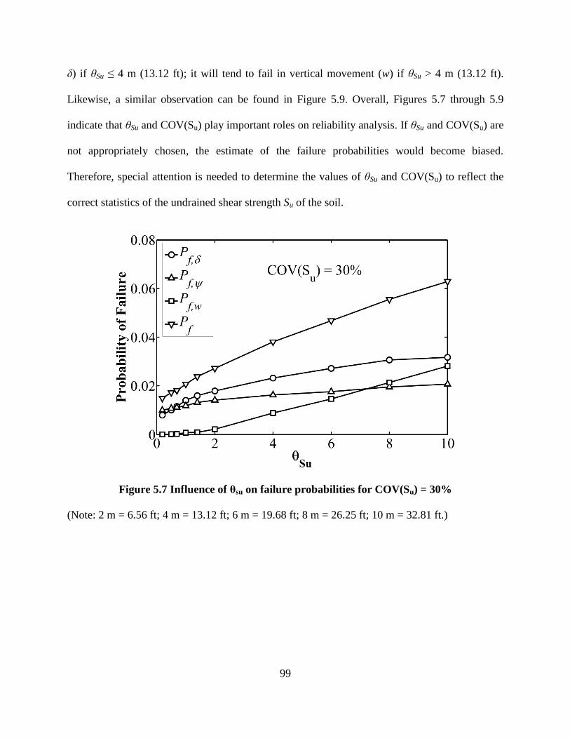
99
δ) if θSu ≤ 4 m (13.12 ft); it will tend to fail in vertical movement (w) if θSu > 4 m (13.12 ft).
Likewise, a similar observation can be found in Figure 5.9. Overall, Figures 5.7 through 5.9
indicate that θSu and COV(Su) play important roles on reliability analysis. If θSu and COV(Su) are
not appropriately chosen, the estimate of the failure probabilities would become biased.
Therefore, special attention is needed to determine the values of θSu and COV(Su) to reflect the
correct statistics of the undrained shear strength Su of the soil.
Figure 5.7 Influence of θsu on failure probabilities for COV(Su) = 30%
(Note: 2 m = 6.56 ft; 4 m = 13.12 ft; 6 m = 19.68 ft; 8 m = 26.25 ft; 10 m = 32.81 ft.)

100
Figure 5.8 Influence of θsu on failure probabilities for COV(Su) = 50%
Figure 5.9 Influence of θsu on failure probabilities for COV(Su) = 70%

101
5.6 Summary and Conclusions
This chapter presents a probabilistic framework to evaluate the serviceability performance
of a drilled shaft. This study addresses the limitations of the current LRFD approach that handles
the serviceability limit state in a deterministic way. In the proposed framework, the uncertainties
that affect the reliability of a designed drilled shaft are identified as the following: soil properties,
material properties, model errors in the soil interaction analysis, performance criteria, and
external loads. Particularly, the spatial variability of soil properties is considered using random
field theory, in which each soil property is statistically characterized by the mean, variance, and
correlation length. The model errors of the load transfer curves are accounted for by introducing
model factors. This chapter concluded with an example, where reliability analysis and
importance analysis are conducted for three failure modes (lateral deflection, angular distortion,
and vertical movement at the top of the pile). Based on the results, the following conclusions are
made:
1. The failure probability of the system, Pf, is greater than those of the individual failure
modes. Besides, Pf is less than the summation of the failure probabilities of the three
individual failure modes. The failure probability of the system may be underestimated
if multiple failure modes are not considered simultaneously. It is recommended to
conduct reliability analysis system-wise if multiple failure modes exist. In the current
LRFD approach, different limit states are considered separately, which leads to an
overestimation of the reliability.
2. The importance analysis of the random variables indicate that the major sources of
uncertainties affecting the reliability of a designed drilled shaft come from external
loads, the allowable displacement, soil property Su, and the model factors of the load

102
transfer curves. The variability in concrete and reinforcement is relatively less
important.
3. Considering the dependence structures of soil properties in reliability analysis is
essential. If the dependence structures of soil properties are ignored or not considered
appropriately, the calculated probability of failure will be biased. Therefore, guidance
regarding how to determine the dependence structures of soil properties is needed.

103
CHAPTER 6. USE OF IMPORTANCE SAMPLING IN RELIABILITY ANALYSIS
6.1 Introduction
Monte Carlo simulation (MCS) is widely used for reliability analysis because of its
mathematical simplicity and robustness. An important application of MCS is to evaluate the
probability of failure Pf, as in the following equation:
0
0 0f
G
P P G f d I G f d
x x x x (6.1)
where P(∙) denotes a probability measure, f(x) denotes the joint probability density function
(PDF) of random vector x, I[∙] denotes an indicator function, G denotes a limit state function, and
failure is denoted as G ≤ 0. A general definition of the limit state function is written as follows:
G C D x x (6.2)
where C and D denote the ―capacity‖ and the ―demand‖ in a broad sense. With the probability of
failure, the reliability index β can be evaluated accordingly:
1 11 f fP P (6.3)
where Φ-1
(∙) denotes the inverse of the cumulative distribution function for the standard normal
variable.
A common problem with the evaluation of the failure probability is that the number of
dimensions in reliability problems may be large, making it difficult to evaluate the numerical
integration (i.e., Equation 6.1) directly. In that case, the integration can be evaluated as the
expectation of the indicator function using Monte Carlo integration (Robert and Casella 2004).
Simply speaking, the probability of failure Pf is approximated as the ratio of the number of
failure events to the total number of samples, as shown in the following equation:
104
,MCS
1
10
n
f i
i
P I Gn
(6.4)
where n is the sample size, the subscript ―MCS‖ indicates that the estimate is evaluated using the
crude MCS method. The indicator function is equal to 1.0 if G is less than or equal to 0;
otherwise, it is zero. It should be noted that in the crude MCS method, the random variables x are
drawn from the joint PDF f.
To guarantee the convergence of Equation (6.4), the sample size n has to be sufficiently
large. According to Ang and Tang (2007), the degree of precision for the estimate of Equation
(6.4) can be measured by its coefficient of variation (COV) δp, which is determined by:
,MCS
,MCS
1 f
p
f
P
n P
(6.5)
Equation (6.5) indicates that the coefficient of variation is affected by the sample size n
and Pf. Based on Equation (6.5), a back-calculation can be used to estimate the sample size n as
follows:
,MCS
2
,MCS
1 f
p f
Pn
P
(6.6)
Based on Equation (6.6), it is concluded that the sample size n is related to Pf and its COV
δp. The smaller δp and Pf are, the larger n is. The probability of failure Pf is typically a small
number. Thus, the sample size n is usually large enough that the convergence of Equation (6.4) is
guaranteed. According to Robert and Casella (2004), a rule of thumb for selecting a sample size
is that n is approximately ten times the reciprocal of the probability level, if the COV for Pf is
taken as 30%. For example, the sample size is at least 10,000 if Pf is equal to 1/1000. A larger
sample size is warranted if a smaller δp is desired. Based on the above discussion, it is well

105
understood that the crude Monte Carlo statistical methods are often computationally expensive as
a result of repetitive evaluation of the indicator function. It becomes even more demanding if the
evaluation of the indicator functions is complex.
In the reliability analysis for axially loaded piles, the authors previously developed a
performance based design approach using the crude MCS method (Fan and Liang 2012). To
improve the computational efficiency of the Monte Carlo method, this research presents an
importance sampling (IS) based algorithm that can be applied to conduct fast reliability
evaluation for an axially loaded pile. The spatial variability of soil properties is considered by
random field modeling, in which each soil property is statistically characterized by the field
mean, the field variance, and the correlation structure. The random fields for soil properties are
simulated by using the local averaging subdivision (LAS) method (Fenton and Griffiths 2008).
This well-accepted load transfer method is employed to evaluate the load-displacement behavior
for the pile. In the proposed importance sampling algorithm, the instrumental function is
constructed by shifting the original PDF such that the mean is at the point having the maximum
probability density of the failure surface. By sampling more heavily from the region of interest
and then scaling the indicator function back by a ratio of probability densities, a faster rate of
convergence can be achieved while maintaining the accuracy of the estimate. Two examples –
one for homogeneous clay sites and the other for non-uniform clay sites – are presented to
illustrate the accuracy and efficiency of the developed importance sampling method.
6.2 Load Transfer Model
The analysis of axially loaded piles is a nonlinear soil-pile interaction problem that is
solved by iterative numerical algorithms. Numerous methods are available to analyze the
response of an axially loaded pile, such as the finite element method and the load transfer
106
method. The load transfer method (e.g., Coyle and Reese 1966) is widely used because of its
accuracy and simplicity. The schematic diagram of the load transfer model is shown in Figure
2.2., and a detailed discussion of the load transfer model can be found in Section 2.1.2.
6.3 Random Field Modeling
Soil properties such as undrained shear strength and friction angle are needed as inputs to
construct the load transfer curves (t-z curves and q-w curves). The soil properties are uncertain
due to intrinsic variability, measurement errors, and interpretation errors. The variations of soil
properties can directly affect the t-z curves and q-w curves in the load transfer model.
Consequently, these variations can exert significant influence on the calculated load-
displacement curve. Therefore, the modeling of soil variability is of great importance in
reliability assessment.
Two statistical parameters, namely the mean μ and variance ζ2, are required to characterize
the variability of a soil property at the point level. The mean measures the center of a dataset
while the variance measures the dispersion from the mean. One commonly used probability
distribution for soil properties is the lognormal distribution (e.g., Griffiths et al. 2009). The use
of lognormal distribution ensures that soil properties are always non-negative. The PDF for
lognormal distribution is given as follows:
2
ln
ln ln 2
lnln
ln1 1, exp
22
x
x x
xx
xf x
x
(6.7)
where μlnx and ζlnx are the distribution parameters. The distribution parameters can be determined
based on the mean μx and the standard deviation ζx, as shown in the following equation:
2
ln 2ln 1 x
x
x
(6.8)

107
2
ln lnln 0.5x x x (6.9)
For mathematical simplicity, it is preferable to have normal variables. By taking the
logarithm, a lognormally distributed random variable can be transformed to a normal variable
with a mean of μlnx and a standard deviation of ζlnx. The advantage of such a transformation will
become clear in the subsequent discussion. It should be noted that other probability distributions
(such as the normal distribution) are possible choices for modeling soil properties.
In addition to the mean and the variance, a third parameter called correlation length θ is
required to characterize the spatial variability of a random variable (Vanmarcke 1977). The
correlation length is needed to define a correlation function, which describes how random
variables are correlated at different separation distances. For example, the correlation function
for Markov process is shown in Equation (2.11) and is adopted herein because of its widespread
use.
6.4 Importance Sampling Method
6.4.1 Mathematical Formulation
Let us reconsider Equation (6.1), which presents a mathematical formulation for the failure
probability. In the crude MCS solution (see Equation 6.4), samples of x are drawn directly from
the PDF of interest (denoted as f in that equation). As alluded to earlier, the probability of failure
is usually a very small number, which means that only a very small portion of samples from the
region of interest can be drawn. Although the remaining samples do not contribute to the
estimation of Pf, they are still used as inputs to evaluate the indicator function. As a result of the
repetitive evaluation for those samples, the rate of convergence is slowed. To address this
deficiency, one possible solution is to draw more samples from the region of interest (i.e., G ≤ 0).
This can be achieved through a carefully devised instrumental function in importance sampling.

108
If the instrumental function is denoted as h, the mathematical representation of importance
sampling for Equation (6.1) can be expressed as:
,IS
1
= 0
1 0
f
ni
i
i i
fP I G h d
h
fI G
n h
xx x
x
x
x
(6.10)
where f(x)/h(x) is the importance sampling quotient and the subscript ―IS‖ indicates that the
estimate is evaluated by importance sampling. Note that the random samples x in Equation (6.10)
are drawn from h(x) instead of f(x). The importance sampling method has minimal constraints. It
only requires that the support of f is contained in that of h such that the variance for the estimate
is finite. Equation 6.10 is very useful, and it gives a different perspective on the estimation of Pf.
By carefully selecting an instrumental function h, more samples are drawn from the region of
interest, resulting in faster convergence. From a statistical point of view, the instrumental
function is introduced to reduce the variance in the estimate in a MCS problem.
6.4.2 Important Considerations
The objective of applying importance sampling is to be able to conduct fast reliability
evaluation without losing accuracy. When applying importance sampling to the reliability
evaluation of axially loaded piles, there are a few fundamental considerations:
1. The number of dimensions in the reliability problem is high, and the IS estimator (i.e.,
Equation 6.10) should give the same unbiased estimate as does the crude MCS method;
2. The IS estimator should yield a fast rate of convergence; and
3. An efficient method for simulating the random samples from the instrumental function
should be available.
109
The first consideration is related to the accuracy of the importance sampling technique,
while the second and the third ones are related to the computational efficiency of the technique.
In the analysis of axially loaded piles, the vertical movement under axial loading is evaluated by
the load transfer method, in which the pile under consideration is discretized into a finite number
of segments. The soil-pile interaction behavior for each segment is characterized by a t-z curve or
a q-w curve. Thus, the number of dimensions is large in importance sampling. A common
concern associated with the high-dimensional importance sampling problem is the question of
whether the importance sampling estimator can converge or not. It is worthwhile to note that the
convergence of the estimate comes with some conditions on h and cannot be taken for granted in
high-dimensional importance sampling. Detailed discussions of those conditions can be found in
Au and Beck (2003). Finally, it is important to note that the simulation of the random samples
should be efficient, as the random samples are used as inputs to evaluate the indicator function
and will directly affect the rate of convergence.
6.4.3 Implementation Scheme
The choice of the instrumental function h is a crucial step, because the instrumental
function would not only directly affect how efficient it is to draw the random samples, but it
would also affect the evaluation of the indicator function and the corresponding importance
sampling quotient. The optimal choice for the instrumental function is determined by the
following equation:
0 0
0opt
f
I G f I G fh
PI G f d
x xx
x x (6.11)
in which the variance of the estimate is equal to zero. Unfortunately, the optimal choice of the
instrumental function is not feasible in practice, because it requires the knowledge of the integral

110
of interest (i.e., Pf), which is unknown! Though not practical, the optimal instrumental function
gives important insights: it demonstrates that 1) hopt covers the entire region of interest and has
no support beyond that region; and 2) hopt is proportional to the original joint PDF f by a factor of
1/Pf in the region of interest, regardless of x. Taking advantage of these insights, the instrumental
function is chosen so that significant probability content from the region of interest can be
covered. It has been suggested that a design point x* can be used to identify the region of interest
(Melchers 1999). The design point x*, which is the point lying on the failure surface which has
the maximum likelihood, is calculated as follows:
0
* arg maxG
f
x x (6.12)
where ―arg‖ is short for argument, and max[∙] denotes the maximum value under the constraint G
= 0. Once the design point is determined, a common strategy is to shift the original PDF f so that
the mean is at the point x* (e.g., Au and Beck 1999; Melchers 1999).
6.4.4 Locating Design Point
The objective of this section is to present the proposed approach for pinpointing the design
point so that the region of interest can be characterized. Based on the well-accepted first order
reliability method (FORM), Low and Tang (2007) have shown a geometric interpretation for the
reliability index in that β is equal to the minimum distance from the failure surface to the origin
in the u-space, where u is standard normal variable. In general, the design point is obtained by
solving a constrained optimization problem. There are numerous algorithms for solving the
optimization problem; among them is the gradient projection method, which has been proven to
be an efficient algorithm to use in searching for the design point (e.g., Der Kiureghian and
Stefano 1991; Der Kiureghian and Liu 1991). The method is summarized below:

111
1. Assume an initial point x0 for x in the x-space and transform it to independent
standard normal variable u = u(x), choosing tolerances δ1 and δ2 for checking convergence.
2. Evaluate the gradient vector α:
1 2
, , ,T
k
G G GG
u u u
u (6.13)
G
G
u
u (6.14)
where ||∙|| measures the Euclidean norm of a vector.
3. Determine search direction v:
T
G
G
uv u u
u (6.15)
4. Assume a step size λ (e.g., λ = 1) and then find a new iteration point unew:
new +u u v (6.16)
5. Check whether convergence is achieved or not:
new 1G u (6.17)
new 2
T u u (6.18)
It is important to note that Equation (6.17) and Equation (6.18) must be satisfied
simultaneously when convergence is obtained.
6. Repeat Steps 2 through 5 until convergence is achieved.
7. Evaluate the reliability index using the design point u*:
newu* u (6.19)
*T u (6.20)
112
It should be noted that the design point x* can be obtained by transforming u* back to the
original space.
6.4.5 Response Surface Method
The objective in using the response surface method is to construct a limit state function
that can be used in the search of the design point. In the load transfer model, there is no explicit
equation for calculating the vertical movement at the top of the pile. The vertical movement is
solved iteratively through the use of numerical algorithms. Therefore, the limit state function
should be established before applying FORM. An example of the limit state function by using
the response surface method is given below:
2
1 2
1 1
ln , ln , , ln ln lnk k
k i i i i
i i
G x x x a b x c x
(6.21)
where a, b and c are regression coefficients, (x1, x2, …, xk) is a vector of random variables, and
ln(∙) denotes the natural logarithm. Note that the logarithms of soil properties are used as
predictor variables in the response surface method. While using other forms of the limit state
function would also be feasible, the use of a quadratic form makes it efficient to evaluate the
gradient vector in the FORM.
6.4.6 Algorithm
Normal variables can be used as an example to illustrate the construction of an
instrumental function. As mentioned earlier, it is assumed that soil properties are lognormally
distributed. Normal variables can be obtained by taking logarithms of the soil properties. For
example, suppose that x=(x1,x2,…,xk)T has a mean vector μ and a covariance matrix C. After the
limit state function and the statistics of the random variables are defined, FORM analysis is
conducted to pinpoint the design point x* (where the center of the instrumental function is at x*).
113
There is little flexibility in choosing the covariance matrix in high-dimensional importance
sampling problem. According to Au and Beck (2003), there are some restrictions on the
covariance matrix. If the covariance matrix for h is not appropriate, the consequence is that the
estimate of Pf will vanish or be biased, particularly in the case of a high-dimensional importance
sampling problem. In order to have an unbiased estimate, the covariance matrix of the
instrumental function h is taken as the same as in f in this study. Now it becomes clear that the
random samples are drawn from ϕ(x*, C) instead of ϕ(μ, C), where ϕ(∙) denotes the joint PDF for
normal variables. The advantage in using a normal distribution is that the joint PDF has an
explicit form, so that it is efficient to use for evaluating the importance sampling quotient.
In summary, the instrumental function is shifted so that the mean is at the design point x*
while the covariance term remains unchanged. In this case, it is anticipated that approximately
one half of the random samples will be drawn from the failure domain. Once the instrumental
function is defined, the importance sampling quotient R is evaluated using the following equation:
1
1
1exp
, 2
1,exp *
2
T
T
- -f
Rh
- -
x C xx Cx
x x x* Cx x* C x x
(6.22)
The variability of the estimator is measured by its COV, which is given by this equation:
2 2 2
,IS,IS
1,IS
,IS
0Var
1E( )
n
i i ffIS i
p f
f
I G R nPPP
n nP
(6.23)
where Var(∙) denotes the variance for the estimate and E(∙) denotes the expectation.
The algorithm for conducting fast reliability evaluation of axially loaded piles is
summarized as follows:

114
1. Define the soil profile of interest and the associated statistics (mean μ and covariance C)
for soil properties.
2. Determine the mechanical properties (EA) of the pile.
3. Define the allowable displacement as the failure criterion.
4. Obtain the design axial load.
5. Construct an approximated limit state function using the response surface method.
6. Search for the design point x* using the described gradient projection method.
7. Construct the instrumental function h(x) = ϕ(x | x*, C).
8. Assume a sample size n (e.g., 300 to 1000) and draw random samples from h(x).
9. Use the realizations of the random samples as inputs to compute the vertical movement of
the pile.
10. Conduct statistical analysis using the realizations of the vertical movement and evaluate
the failure probability using Equation (6.22) and Equation (6.23).
A computer program has been developed based on the above algorithm and has been tested. The
following examples are presented to illustrate the proposed approach.
6.5 Examples
6.5.1 Example 1: Drilled shaft in a homogeneous soil deposit
The objective of Example 1 is to demonstrate the accuracy of the developed importance
sampling algorithm. Consider a drilled shaft with a 1.10-m (3.61 ft) diameter and a 8.0-m (26.25
ft) length in a homogeneous clay soil deposit that is subjected to compression force Q of 1300
KN (292.24 kips). The adopted failure criterion is a vertical displacement ya of 25 mm (1 in).
Both ya and Q are deemed deterministic in this example, although they can be treated as random
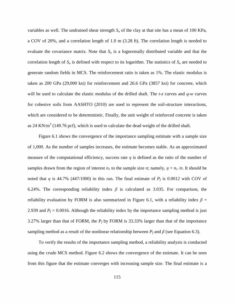
115
variables as well. The undrained shear strength Su of the clay at that site has a mean of 100 KPa,
a COV of 20%, and a correlation length of 1.0 m (3.28 ft). The correlation length is needed to
evaluate the covariance matrix. Note that Su is a lognormally distributed variable and that the
correlation length of Su is defined with respect to its logarithm. The statistics of Su are needed to
generate random fields in MCS. The reinforcement ratio is taken as 1%. The elastic modulus is
taken as 200 GPa (29,000 ksi) for reinforcement and 26.6 GPa (3857 ksi) for concrete, which
will be used to calculate the elastic modulus of the drilled shaft. The t-z curves and q-w curves
for cohesive soils from AASHTO (2010) are used to represent the soil-structure interactions,
which are considered to be deterministic. Finally, the unit weight of reinforced concrete is taken
as 24 KN/m3 (149.76 pcf), which is used to calculate the dead weight of the drilled shaft.
Figure 6.1 shows the convergence of the importance sampling estimate with a sample size
of 1,000. As the number of samples increases, the estimate becomes stable. As an approximated
measure of the computational efficiency, success rate η is defined as the ratio of the number of
samples drawn from the region of interest n1 to the sample size n; namely, η = n1 /n. It should be
noted that η is 44.7% (447/1000) in this run. The final estimate of Pf is 0.0012 with COV of
6.24%. The corresponding reliability index β is calculated as 3.035. For comparison, the
reliability evaluation by FORM is also summarized in Figure 6.1, with a reliability index β =
2.939 and Pf = 0.0016. Although the reliability index by the importance sampling method is just
3.27% larger than that of FORM, the Pf by FORM is 33.33% larger than that of the importance
sampling method as a result of the nonlinear relationship between Pf and β (see Equation 6.3).
To verify the results of the importance sampling method, a reliability analysis is conducted
using the crude MCS method. Figure 6.2 shows the convergence of the estimate. It can be seen
from this figure that the estimate converges with increasing sample size. The final estimate is a

116
Pf of 0.0013 with a COV of 5.24%. Note that the success rate is only 0.13% (i.e., 390/300,000
where n = 300,000) in this run for the crude MCS method, which is much lower than that for the
importance sampling method (44.7%).
Figure 6.1 Reliability evaluations by IS method and FORM for Example 1
0 200 400 600 800 10000
0.5
1
1.5
2
2.5
3x 10
-3
Number of Samples
Pro
ba
bil
ity
of
Fa
ilu
re
Importance samplingP
f,IS = 0.0012
COV = 6.13%
= 3.035
FORMP
f,FORM = 0.0016
= 2.939
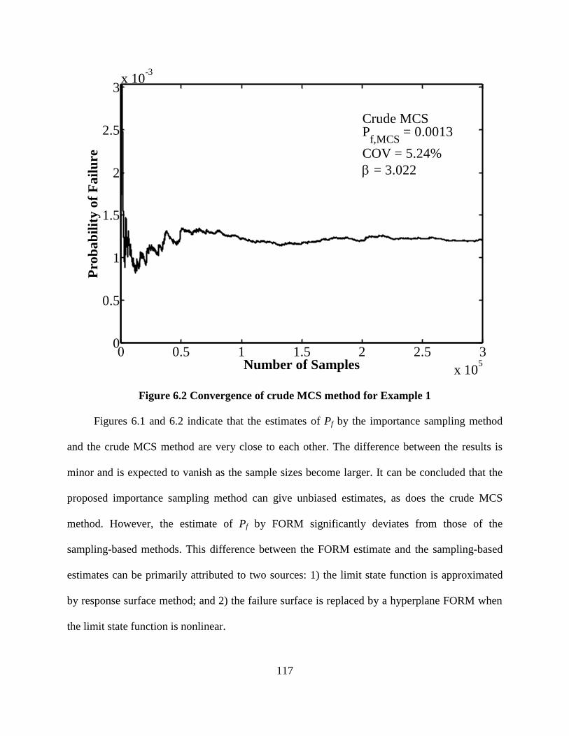
117
Figure 6.2 Convergence of crude MCS method for Example 1
Figures 6.1 and 6.2 indicate that the estimates of Pf by the importance sampling method
and the crude MCS method are very close to each other. The difference between the results is
minor and is expected to vanish as the sample sizes become larger. It can be concluded that the
proposed importance sampling method can give unbiased estimates, as does the crude MCS
method. However, the estimate of Pf by FORM significantly deviates from those of the
sampling-based methods. This difference between the FORM estimate and the sampling-based
estimates can be primarily attributed to two sources: 1) the limit state function is approximated
by response surface method; and 2) the failure surface is replaced by a hyperplane FORM when
the limit state function is nonlinear.
0 0.5 1 1.5 2 2.5 3
x 105
0
0.5
1
1.5
2
2.5
3x 10
-3
Number of Samples
Pro
ba
bil
ity
of
Fa
ilu
re
Regular MCSp
f = 0.0013
COV = 5.24%
= 3.022
Crude MCSP
f,MCS = 0.0013
COV = 5.24%
= 3.022

118
In order to investigate the influence of the correlation length θ (a measure of the
correlation structure of soil properties) and the axial load Q; both θ and Q are varied while other
parameters remain fixed. Figure 6.3 shows the relationships between Pf and the two parameters.
It can be observed that Pf increases with increasing axial load. For a given Q, there is a
significant variation in Pf if θ is different. It is worthwhile to note that the difference in Pf could
be several orders of magnitude, particularly when Pf is a very small number (e.g., Pf ≤ 1/1000).
It can be concluded that considering θ would be critical in reliability analysis. Furthermore, if the
correlation length is not properly accounted for, the estimate of Pf would probably become
biased.
Figure 6.3 Influences of θ and Q
1000 1100 1200 1300 1400 1500 1600 1700 180010
-6
10-5
10-4
10-3
10-2
10-1
100
Q, KN
Pf
= 0.5 m
= 1 m
= 2 m
= 4 m
= 6 m

119
6.5.2 Example 2: Drilled shaft in heterogeneous soil deposit
The objective of Example 2 is to demonstrate the efficiency of the developed importance
sampling method in a non-homogeneous clay deposit. Consider a drilled shaft that is 1.0 m (3.28
ft) in diameter and 10.0 m (32.81 ft) in length that is subjected to a compression force of 1400
KN. In contrast to the previous example, the mean of Su (denoted as μSu) is varied over the depth
z (in meter): the μSu is 90 KPa (13.05 psi) for the topmost 2.5 m (8.2 ft) of the shaft and then
linearly increases at depths below 2.5 m (8.2 ft) as described in the equation μSu = 83.478+2.609z
(KPa). The standard deviation of Su is 18 KPa (2.61 psi) along the depth and the correlation
length θ = 1.2 m (3.94 ft). The failure criterion in terms of vertical displacement is 25 mm (1 in).
The reinforcement ratio is taken as 1%. The elastic modulus is taken as 200 GPa (29,000 ksi) for
reinforcement and 26.6 GPa (3857 ksi) for concrete. The same t-z curves and q-w curves for
cohesive soils from AASHTO (2010) are used to represent the soil-pile interactions.
Figure 6.4 shows the convergence of the estimate using the proposed IS based method. The
final estimate is 0.00089 with COV of 6.11%, with a corresponding value for β of 3.122. The
success rate is η = 45.7% (457/1000). For comparison, the reliability evaluation by FORM is also
summarized in Figure 6.4, shows that β is equal to 2.984 (i.e., Pf = 0.0014). To validate the
results of the importance sampling method, a reliability analysis using the crude MCS method is
conducted, and the convergence of the MCS estimate with a sample size of 400,000 is presented
in Figure 6.5. The estimate of Pf by the crude MCS method is 0.00086 with a COV of 5.37%,
and the corresponding β of 3.133, which is very close to that of the importance sampling method.
Although the reliability indices evaluated by different methods are close to each other, the Pf
evaluated by FORM is approximately 60% larger than those of the sampling-based methods!
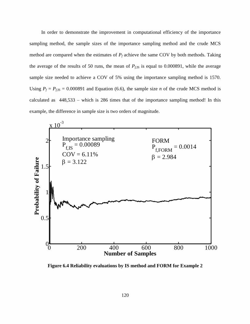
120
In order to demonstrate the improvement in computational efficiency of the importance
sampling method, the sample sizes of the importance sampling method and the crude MCS
method are compared when the estimates of Pf achieve the same COV by both methods. Taking
the average of the results of 50 runs, the mean of Pf,IS is equal to 0.000891, while the average
sample size needed to achieve a COV of 5% using the importance sampling method is 1570.
Using Pf = Pf,IS = 0.000891 and Equation (6.6), the sample size n of the crude MCS method is
calculated as 448,533 – which is 286 times that of the importance sampling method! In this
example, the difference in sample size is two orders of magnitude.
Figure 6.4 Reliability evaluations by IS method and FORM for Example 2
0 200 400 600 800 10000
0.5
1
1.5
2
x 10-3
Number of Samples
Pro
ba
bil
ity
of
Fa
ilu
re
Importance samplingP
f,IS = 0.00089
COV = 6.11%
= 3.122
FORMP
f,FORM = 0.0014
= 2.984

121
Figure 6.5 Probability of failure by crude MCS method for Example
In order to further investigate the performance of the proposed importance sampling
method at different probability levels, the axial load Q is varied while other parameters in this
example remain unchanged. Figure 6.6 shows the sample sizes that correspond to a COV of 5%
for the estimates of Pf and the associated success rates when the results of 50 runs are averaged.
As a result of the variation in the axial load, the probability of failure increases from 2.06×10⁻⁶
to
0.74. It can be seen that the average sample size of the importance sampling method slightly
decreases from 2,555 to 518 until Pf ≥ 42.5%. Meanwhile, the average sample size of the crude
MCS method decreases from 1.94×10⁸ to 140. In this example, the difference in sample size
between the two methods is at least two orders of magnitude when Pf ≤ 1/1000. Moreover, the
difference becomes more noticeable when Pf becomes smaller.
0 0.5 1 1.5 2 2.5 3 3.5 4
x 105
0
0.5
1
1.5
2
2.5
x 10-3
Number of Samples
Pro
ba
bil
ity
of
Fa
ilu
re
Crude MCSP
f,MCS = 0.00086
COV = 5.37%
= 3.133
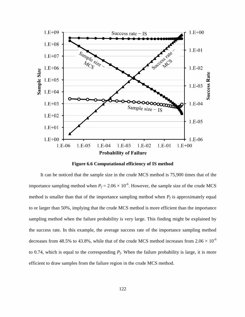
122
Figure 6.6 Computational efficiency of IS method
It can be noticed that the sample size in the crude MCS method is 75,900 times that of the
importance sampling method when Pf = 2.06 × 10⁻⁶
. However, the sample size of the crude MCS
method is smaller than that of the importance sampling method when Pf is approximately equal
to or larger than 50%, implying that the crude MCS method is more efficient than the importance
sampling method when the failure probability is very large. This finding might be explained by
the success rate. In this example, the average success rate of the importance sampling method
decreases from 48.5% to 43.8%, while that of the crude MCS method increases from 2.06 × 10⁻⁶
to 0.74, which is equal to the corresponding Pf. When the failure probability is large, it is more
efficient to draw samples from the failure region in the crude MCS method.

123
Based on the comparison in Example 2, it is clear that the importance sampling method
brings considerable improvement in computational efficiency over the crude MCS method,
particularly when Pf is a very small number. However, instead of the importance sampling
method, the crude MCS method should be used if Pf is large (e.g., Pf ≥ 50%), from the standpoint
of computational efficiency.
6.6 Summary and conclusions
The crude MCS method is known to be computationally demanding. In order to increase
the computational efficiency, this research presents an importance sampling–based algorithm
that can be applied to conduct fast reliability evaluation for axially loaded piles. The spatial
variability of soil properties is considered by random field modeling, which characterizes the
random field of a soil parameter by factoring the field mean, the field variance, the probability
distribution, and the correlation structure into the model. In importance sampling, the
instrumental function is constructed by shifting the original PDF such that the mean is at the
point having the maximum probability density of the failure surface. A computer program has
been developed in order to apply the proposed algorithm for conducting reliability analysis.
Based on the two examples of drilled shaft design presented in this chapter, the following
conclusions can be made:
1. The proposed importance sampling method gives the same unbiased estimate of the
failure probability as the crude MCS method.
2. The proposed importance sampling method is much more efficient than the crude MCS
method when evaluating a small probability of failure (e.g., Pf ≤ 1/1000). By drawing
more samples from the region of interest, the proposed method will achieve a faster rate
124
of convergence. With the same sample size, the estimate obtained by using the
importance sampling method would have a much smaller coefficient of variation than the
estimate obtained by the crude MCS method.
3. The importance sampling method is highly efficient in variance reduction for the estimate,
and it is recommended to use the importance sampling method in the evaluation of small
probabilities of failure.
4. It is demonstrated that the probability of failure is sensitive to the correlation length, θ. If
θ is not considered in reliability assessment, the estimated probability of failure would
probably be biased. Therefore, considering correlation length is warranted in the
reliability analysis of deep foundations.
5. The probability of failure evaluated by the commonly used first order reliability method
(FORM) significantly deviates from those of Monte Carlo statistical methods, although
the reliability index by FORM is close to those of Monte Carlo statistical methods. The
differences in the failure probabilities between FORM and Monte Carlo statistical
methods are primarily attributed to the approximation of the limit state function in the
response surface method and the linear truncation of the limit state function in the FORM.
125
CHAPTER 7. SPATIAL VARIABILITY OF SOIL PROPERTIES
7.1 Introduction
As a methodology of reliability based design (RBD), performance-based design
approaches (Fan and Liang 2012, 2013a, 2013b) have been proposed in which the design criteria
are defined in terms of allowable displacements. For drilled shaft under axial loading, the design
criterion is defined with respect to the vertical movement (w) at the top of the shaft. For drilled
shaft under lateral loading, the design criterion is defined with respect to the lateral deflection (δ)
and the angular distortion (ψ) at the top. If any of the displacements (δ, ψ and w) is greater than
the corresponding displacement, failure is to occur. That is
1, for
,0, for
a
a
a
d dI d d
d d
(7.1)
where I(∙) is an indicator function, d = δ, ψ or w, and da denotes the corresponding allowable
displacement. In the proposed approaches, Monte Carlo simulation (MCS) is applied to estimate
the probability of failure Pf,d
,
1
1 K
f d i
i
P IK
(7.2)
where K is the number of simulations. When the number of simulations is sufficiently large, the
estimate in Equation (7.2) will approach its exact value. The advantage of using MCS method is
that the estimate in Equation (7.2) is unbiased. Moreover, it is mathematically straightforward.
In order to calculate the probability of failure, the uncertainties associated with soil
properties need to be accounted for. In the proposed performance based design approaches, the
soil properties are modeled as random fields which are statistically characterized by a mean μ, a

126
standard deviation ζ and a correlation length θ. The correlation length is needed to define a
correlation function. For example, the one-dimensional Markovian correlation function is given
below
2
, exp
(7.3)
where ρ(∙) gives the correlation coefficient between two points and η is the separation distance
between the two points. The mean measures the center of a dataset, the variance measures the
dispersion from the mean, and the correlation length measures how rapidly a random field varies
in space. It has been demonstrated that the statistical descriptors (μ, ζ and θ) have a significant
impact on Pf,d and the consideration of θ is important in reliability analysis (see Fan and Liang
2012, 2013a).
In RBD, the probabilistic model of soil profiles is as important as the computational
methods of reliability analysis. The stochastic nature of the soils would directly influence the
response of geotechnical structures to external loads, thus affecting the results of the reliability
analysis. A realistic probabilistic model for soils is an essential part of the input to the
computational methods for the reliability analysis of any geotechnical structure. As a part of the
performance-based design methodology, it is necessary to develop statistical guidelines to
characterize the uncertainties of soil profiles. The objectives of this study include:
1. To develop computational methods of determining the statistical descriptors (μ, ζ and θ)
of a random field for a soil property.
2. To identify the soil stratifications at a given location;
To make the computational methods usable to practicing engineers, data from standard
penetration test (SPT) will be used as a means to estimate the statistical descriptors. SPT is
127
widely used in subsurface investigations, and soil samples can be retrieved during testing. The
advantage of using SPT is that the retrieved soil samples allow for identification of soil
stratification. The soil stratifications would dictate the use of the load transfer curves that may
differ from one soil to another. It should be noted that the identification of soil stratification is as
important as the determination of the statistical descriptors, because the knowledge of soil
stratifications would directly affect the modeling of the soil-structure interaction. As a result, the
displacements of drilled shafts under axial and lateral loads would be influenced, thus affecting
the calculation of the failure probability. In this research, the identification of soil stratifications
and the computational methods to determine the statistical descriptors will be introduced. Finally,
real data from a site investigation will be used as an example to demonstrate the proposed
approach.
7.2 Computational Methods
In the proposed performance-based design methodology, each soil property such as
undrained shear strength (Su) for clay and effective friction angle (ϕ′) for granular soils is
modeled as a random field which is statistically characterize by a mean μ, a standard deviation ζ,
and a correlation length θ. In order to accurately determine the statistical descriptors (μ, ζ and θ)
of a random field, a subsurface investigation should be performed on the construction site and a
certain amount of soil data needs to be gathered to conduct a realistic statistical analysis. Note
that in a subsurface investigation, the cone penetration test (CPT) and the standard penetration
test are the most commonly used tests. In CPT, the cone tip resistance is recorded at every 2-cm
or 5-cm interval and is measured continuously along the depth. Because of the nature of the data,
CPT data may be more amenable to statistical analysis and probabilistic modeling. The random
field based modeling for CPT data is available (see Fenton 1999). Unfortunately, SPT data is

128
quite different from CPT data. In SPT, the blow count is recorded for a 15-cm (6-in.) interval and
may not be measured continuously. It is quite common that the blow counts may be missing for
some intervals along the depth. Moreover, there are many factors that affect the SPT and its
results (Sabatini et al. 2002), which make it difficult to repeat the SPT results. As a result, the
analytical method in (Fenton 1999) for CPT data does not work for SPT data in most cases.
However, in some construction projects, only the SPT data is available, and the CPT data is not
available because of the cost of conducting the test. In order to make the developed performance-
based design approach usable to those projects, the statistical guidelines and the computational
methods designated to SPT data should be developed.
The objective of this section is to develop a probabilistic model for SPT data and
determine the statistical descriptors of soil properties using SPT data. The following steps are
taken:
1. Two commonly-used empirical correlations with SPT data are employed to obtain an
estimate of the soil strength parameter (Su and ϕ′) that will be viewed as observations in
Bayesian approach.
2. The statistical descriptors (μ, ζ and θ) are parameterized and a probabilistic model is
established to evaluate the probability of observing the SPT data.
3. Given the SPT data, Bayesian approach is applied in which the statistical descriptors (μ,
ζ and θ) are the parameters of the probabilistic model.
4. Markov chain Monte Carlo is applied to draw samples of μ, ζ and θ, according to the
established probabilistic model in Step 3.
5. Statistical analysis is conducted using the samples of μ, ζ and θ, and the estimates of μ,
ζ and θ can be obtained accordingly.

129
7.2.1 Correlations with SPT Data
In SPT, only the second and third blow counts (denoted as N1 and N2) are summed to
obtain the N value, where N = N1 + N2. Note that the N value can be converted to undrained shear
strength for cohesive soils or effective friction angle for granular soils, employing commonly
used empirical correlations (see Das 2011):
0.72
600.29u aS N p (7.4)
1 60
0
tan
12.2 20.3a
N
p
(7.5)
where N60 (N60 = N∙ER/60 where ER is the energy efficiency) is the N value corrected to 60%
energy efficiency, pa is the atmospheric pressure (pa = 101.325 KPa), tan-1
(∙) denotes the inverse
tangent, and ζ′0 is the effective vertical stress. Note that other correlation equations may be used
to obtain Su or ϕ′. It is recognized that the correlation equations have model error. However, the
calibration of the model error is beyond the scope of the study.
7.2.2 Bayesian Approach
Because of the nature of the data, the method of moments in which the samples are
averaged to determine the mean and variance may not work well on SPT data. In SPT, the blow
counts are recorded along the depth, which gives a rough indication of the soil strength. It is well
understood that soil properties along the depth may change for a variety of reasons. For example,
the undrained shear strength of normally consolidated clay may increase with depth, as a result
of the increasing confining stress. In this case, if the samples of undrained shear strength
obtained at different elevations are used to conduct a pooled statistical analysis directly, the
130
estimate of the mean will be probably erroneous and the associated standard deviation would be
overestimated! Furthermore, the sample size of the blow counts for a particular geological
stratum may be limited, depending on the thickness of the soil stratum. There is one blow count
for every 0.152-m (6 in.) interval. Although there may be multiple soil borings at the
construction site, the N values collected at different locations should not be pooled to form a
larger sample size. This is because the samples from different locations may not come from the
same population, from the standpoint of statistics. Hence, it may be problematic to directly
evaluate the statistical averages using the method of moment.
As an alternative to the method of moments, Bayesian approach can be applied to model
the uncertainties of SPT data. The objective of applying Bayesian approach is to estimate the
statistical descriptors (μ, ζ and θ) using SPT data. In this study, the parameters of interest are λ =
(μ, ζ, θ) and will be treated as random variables in the Bayesian approach. Given any
observational data X, the posterior probability density distribution (PDF) of λ can be expressed
as
|f c L f X (7.6)
where f′(λ) and f″(λ) are the prior PDF and posterior PDF, respectively; c is a normalizing
constant such that the integration of f″(λ) over the entire space would be unity; and L(λ|X) is the
likelihood function that gives the probability of observing X given that the parameters of the
underlying probabilistic model is λ.
To implement the Bayesian approach, observational data and a probabilistic model of the
data are needed. In this study, the observational data is the estimated soil properties (Su and ϕ′)
that are converted using the empirical correlations. In order to establish a probabilistic model for
the SPT data, three assumptions are introduced:
131
A1. Each N value (450-mm interval) is considered as a unit, and the corresponding second
and the third blow counts (N1 and N2) of the unit are used as two observations of the
soil properties in the Bayesian approach;
A2. The soil properties are second-order stationary in the unit, that is, the mean and the
standard deviation are constant over the interval; and
A3. The soil properties are lognormally distributed.
As indicated in Assumption A1, there are two blow counts (N1 and N2) in a unit. Since
each blow count just corresponds to a 15-cm interval while the SPT N value corresponds to a 30-
cm interval, an ―equivalent‖ N60 is defined as
60 2 , 1,260
i
ERN N i (7.7)
where N′60 is the equivalent N60, and ER is the energy efficiency same as in N60 = N∙ER/60. With
the equivalent N60, the soil properties (Su and ϕ′) can be obtained according to the empirical
correlations.
With Assumption A2 and A3, the probability of observing the SPT data (N1 and N2) can be
expressed as
2 22
1 1| exp
2 12 1
TL
X X R X (7.8a)
1
1
R (7.8b)
where L(∙) denotes the likelihood function, X = [ln(x1), ln(x2)]T where x = Su or ϕ′, the subscripts
―1‖ and ―2‖ of x corresponds to N1 and N2, respectively; ln(∙) denotes the natural logarithm and
exp(∙) denotes the exponential function; μ and ζ are the mean and the standard deviation of the
random variable ln(x), respectively; the superscript ―T‖ denotes transpose; and ρ is the
132
correlation coefficient between ln(x1) and ln(x2). Indeed, ρ is a function of the parameter θ, that is,
ρ = ρ(θ). Note that the exact form of ρ(θ) is dependent upon what kind of correlation function is
in use. An example of the correlation function is given in Equation (7.3), where τ is equal to
0.152 m (6 in.). As a result of the functional relationship between the correlation coefficient ρ
and θ, the parameter vector λ is re-written as (μ, ζ, ρ) for notational simplicity. Since the soil
properties are lognormally distributed according to Assumption A3, the logarithms of Su or ϕ′
will be normally distributed. It is preferable to have normally distributed variables, because an
analytical form of the joint probability density function is available. Now the advantage of
invoking Assumption A2 and A3 become clear.
In addition to the likelihood function, the prior PDF of the parameters λ = (μ, ζ, ρ) should
be determined. Prior to the statistical analysis, the knowledge of the parameters is limited. In
Bayesian statistics, it is common to assume that the parameters of interest (μ, ζ and ρ) follow
uniform distributions or normal distributions. In most cases, there are no general guidelines to
determine the corresponding distribution parameters. Rough estimates of the parameters based
on the observational data should be adequate. In the context of SPT, the soil properties (x = Su or
ϕ′) can be estimated according to the empirical correlations with the N value. With the estimated
soil properties, the mean μx and the standard deviation ζx of the soil properties may be assumed
according to those used in the study by Phoon and Kulhawy (1999). Since the soil properties are
lognormally distributed, the distribution parameters (μlnx and ζlnx) of ln(x) can be calculated as
2
ln2 2
ln xx
x x
(7.9)
2 2
ln ln 1x x x (7.10)

133
Once the distribution parameters are determined, the range of μlnx and ζlnx can be roughly
estimated. Physically, the correlation coefficient between adjacent soil properties should be
positive. Thus, the prior PDF of the parameters λ can be expressed as follows:
, ,f f f f f (7.11)
where fμ(∙), fζ(∙), and fρ(∙) denote the PDF of μ, ζ, and ρ, respectively. Note that other probability
distributions may be assumed as the prior PDF for μ, ζ and ρ, depending on the setting of the
problem.
7.2.3 Implementation Using Markov Chain Monte Carlo
The objective of applying Markov chain Monte Carlo (MCMC) is to draw the samples of μ,
ζ, and ρ according to the formulation of the Bayesian approach presented previously. The
advantage of using MCMC is that the normalizing constant c in Equation (7.8) can be avoided.
In MCMC, the samples can be drawn directly without knowing c. More importantly, it is more
straightforward to conduct statistical analysis using the resulting samples generated through
MCMC, instead of using numerical integration with respect to the posterior probability density
function. The advantages of using MCMC will be clear in the following paragraphs. The details
of MCMC can be found in Robert and Casella (2004). Figure 7.1 shows the flow chart of the
computational method. The following steps are taken to implement the computational method:
1. Establish the likelihood function (see Equation 7.8a).
2. Assume a prior PDF of the parameters (see Equation 7.11).
3. Assume an initial point of the parameters to start the simulation of the parameter using
MCMC.
4. Conduct statistical analysis of the resulting samples.
5. Obtain the estimates of μ, ζ and ρ.
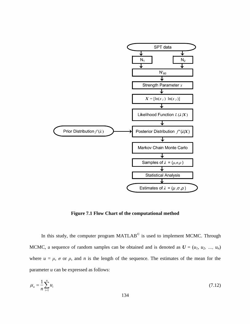
134
Figure 7.1 Flow Chart of the computational method
In this study, the computer program MATLAB©
is used to implement MCMC. Through
MCMC, a sequence of random samples can be obtained and is denoted as U = (u1, u2, …, un)
where u = μ, ζ or ρ, and n is the length of the sequence. The estimates of the mean for the
parameter u can be expressed as follows:
1
1 n
u i
i
un
(7.12)

135
where μu denotes the mean of u. The mean of the samples may be used as an estimate of the
parameter. Note that the estimate of θ can be obtained by plugging the mean of ρ into Equation
(7.3).
7.3 Geostatistical Analysis
The methods of estimating statistical parameters (μ, ζ and θ) are discussed previously.
Once the three statistical parameters are available, and the soil variability model is defined.
However, in practice, drilled shafts may not be installed at exactly the same location where soils
are sampled for analysis. The objective of this section is to present the geostatistical principles
that can be applied to interpret the soil profile.
A number of geostatistical techniques called kriging are available for estimating unknown
values based on available observations. Kriging is a collection of generalized linear regression
methods which includes ordinary kriging, polygon, triangulation, local sample mean, and inverse
distance method. Basically, a kriging estimator is a linear combination of known or observed
data. The accuracies and comments about these methods can be referred to in the literature
(Isaaks and Srivastava 1989). For illustration purposes, the inverse distance method is presented
as follows:
0
1
m
j j
j
T w T
(7.13a)
1
, 1,2, ,m
v v
j j i
i
w l l j m
(7.13b)
where T0 is an estimate of the unknown value, Tj is the j-th observation with a distance of lj to the
desired location, wj is the relative weight for the j-th observation, m is the number of
observations, and v is a power term that can be adjusted. A different u would usually result in a
136
different estimate. If v is taken as 1.0, the weights are inversely proportional to the distance. In
the inverse distance method, the estimator is a weighted mean of nearby samples. The advantage
of using inverse distance method is that more weight is given to the closest samples and only the
distances are needed to determine the weights. It should be noted that kriging techniques other
than the inverse distance method may be possible alternatives, depending on the data at hand and
the specific settings of the problem.
Note that in Equation (7.13a), the term ―T‖ is a quantity of interest. For example, it can be
the thickness of a soil layer, a strength parameter, or a statistic of soil properties. In application,
the distances between the desired location and the locations that have observations need to be
determined first. Once that information is obtained, the relative weight of each observation is
evaluated by assuming a power term v.
7.4 Example
The example is taken from a project that is intended to create a grade-separation between
State Route 58 and the existing CSXT Railroad tracks in Wellington, Ohio. To carry the railroad
tracks, a bridge was constructed and the bridge is supported by two abutments, each of which
consists of 17 drilled shafts. One of the drilled shafts is shown in Figure 7.2. In this figure, the
locations where SPT was conducted are denoted as BR1 and BR2 The dead axial load applied to
the drilled shaft is QD = 351.39 KN (79 kips), while the live axial load is QL = 631.62 KN (142
kips). The lateral load of VD = 162.72 KN (36.58 kips) applied at the top of the drilled shaft
results from the lateral earth pressure and should be considered as dead load. All the given loads
are unfactored. The load eccentricity of the lateral load is 1.69 m (5.54 ft) and will be used to
calculate the bending moment at the top of the drilled shaft. The elevations at the top at the three
locations are 258.3 m (847.44 ft) and 258.0 m (846.46 ft), respectively. The maximum allowable
137
displacements are specified as 0.0254 m (1 in) for both vertical movement and lateral deflection.
The angular distortion at the top is not considered in this example. Using load and resistance
factor design approach, the final design is a drilled shaft that is 25.30 m (83 ft) in length and 1.07
m (42 in) in diameter. The cross section is reinforced by a total of 20 No. 11 rebars, and the
cover thickness is 7.6 cm (3 in.). Note that the elevation of the top of the drilled shaft is 253.0 m.
Hence, the drilled shaft does not penetrate through the topmost three soil layers.
7.4.1 Subsurface Investigation
It is known that the site lies within the glaciated portion of Ohio where the topmost soils
consist of moraine materials. From the site investigation, the general subsurface conditions can
be described in the descending order as follows:
1. 0.05 m (2 in) to 0.30 m (0.99 ft)of topsoil;
2. 0.91 m (2.99 ft) to 5.18 m (17 ft) of stiff to very hard dark brown mottled with gray silt
and clay;
3. 2.60 m (8.53 ft) to 8.08 m (26.51 ft) of hard gray silt, and soft to medium stiff brownish
gray clay;
4. 1.98 m (6.5 ft) to 4.72 m (15.49 ft) of very stiff to hard brown and gray clay;
5. 5.50 m (18 ft) to 9.14 m (30 ft) of stiff to hard gray and brown clay, silty clay and some
silt;
6. SPT was terminated at the depth of 30.39 m (99.7 ft) at BR1 and 28.99 m (95.1 ft) at
BR2 after very dense sand and silt.
The SPT data are shown in Figure 7.3. The ground water is found at the depth of 13.10 m
(43 ft) at BR1 and 20.7 m (67.91 ft) at BR2.

138
Figure 7.2 Layout of borings and drilled shaft
Figure 7.3 SPT data of the project
139
7.4.2 Random Field Modeling Using SPT Data
The proposed method is applied to establish the probabilistic model for soil parameters.
For demonstration purposes, the N value from a silt and clay layer at BR1 is used as input where
N1 = 2, N2 = 2, and ER = 75%. Hence, the corresponding N′60 = 5 for both N1 and N2. The
resulting undrained shear strength of x = 93.62 KPa (13.57 psi) is obtained using Equation (7.4).
Next, the observational vector X = [ln(93.62), ln(93.62)] = [4.54, 4.54]. Plugging X into
Equation (7.8a), the likelihood function L(λ|X) can be obtained. According to Phoon and
Kulhawy (1999), the COV of undrained shear strength can be assumed as 25%. Taking
advantage of the lognormality assumption for soil properties and applying Equation (7.9) and
Equation (7.10), the distribution parameters of undrained shear strength can be calculated as μlnx
= 4.414 and ζlnx = 0.500 given μx = 93.62 KPa (13.57 psi) and ζx = 50.00 KPa (7.25 psi).
Following the steps shown in the flow chart, it is assumed that μ follows a normal distribution
with mean of 4.414 and COV of 40%, ζ follows truncated normal distribution (ζ > 0) with mean
of 0.500 and COV of 40%, and ρ follows the standard uniform distribution. With all these inputs,
the built-in function ―slicesample‖ of MATLAB©
is run to implement MCMC. Accordingly, the
random samples of μ, ζ, and ρ can be drawn and shown in Figure 7.4. In order to reduce the
effect of the initial value that is needed to start the Markov chain, the first 200 samples are
discarded. It can be seen from Figure 7.4 that the samples generated by MCMC converge to the
posterior distribution. Figure 7.5 show the posterior marginal cumulative distribution functions
(CDF) of μ, ζ and ρ. It can be seen that the CDFs of μ and ρ become steeper with the
incorporation of the observational data. However, the posterior CDF of ζ is almost the same as
the prior CDF. These observations indicate that the incorporation of the observational data is
effective in reducing the variability of μ and ρ but is ineffective for ζ. The mean values of μ, ζ,
140
and ρ are 4.549, 0.502 and 0.663, respectively. The resulting correlation length θ can be
calculated as 0.742 m (2.43 ft) by plugging a ρ value of 0.666 into Equation (7.3). By employing
Equation (7.9) and Equation (7.10), the mean and the standard deviation of the undrained shear
strength are determined to be 107.204 KPa (15.54 psi) and 57.353 KPa (8.31 psi), respectively.
The same computational procedures can be repeated for the remaining SPT data. The
computational results for the boring are presented in Table 7.1 for BR1 and in Table 7.2 for BR2;
in these tables, the ―Soil Strength‖ column gives the values for the undrained shear strength or
the effective friction angle that are calculated according to the empirical correlations. Moreover,
the ―μx‖ column gives the local average of soil properties for the interval in SPT, while the ―ζx‖
column gives the corresponding standard deviation of the soil properties. It can be noticed from
these tables that each of the values for the soil strength x is close to the corresponding μx,
indicating that the proposed computational method can preserve the local average of the soil
properties and the spatial trend of soil properties. This is an advantage of the proposed method.
Additionally, the correlation length θ also has some variations, and these are related to the
variation of the correlation coefficient ρ. The larger ρ is, the longer θ will be.

141
Figure 7.4 Random samples generated by MCMC
3
4
5
6
0
0.2
0.4
0.6
0 1000 2000 3000 4000 5000 6000 7000 8000 9000 100000
0.5
1
No. of Iterations

142
Figure 7.5 Posterior marginal CDFs of μ, σ and ρ

143
Table 7.1 Statistics of Soil Properties at BR1
Elevation
(m) x
Soil
Strength μ ζ ρ θ (m) μx ζx
257.4 Su 93.621 4.549 0.502 0.663 0.742 107.204 57.353
256.5 ϕ′ 39.987 3.688 0.111 0.536 0.489 40.222 4.473
255.8 Su 218.740 5.360 0.285 0.392 0.326 221.553 64.375
255.0 Su 276.494 5.605 0.233 0.359 0.298 279.323 65.931
254.2 ϕ′ 39.877 3.681 0.108 0.557 0.521 39.932 4.330
252.9 ϕ′ 35.769 3.570 0.131 0.460 0.392 35.821 4.726
252.4 ϕ′ 40.291 3.698 0.106 0.579 0.559 40.575 4.317
252.0 ϕ′ 30.333 3.410 0.131 0.666 0.750 30.523 4.026
251.5 ϕ′ 32.418 3.480 0.124 0.668 0.756 32.710 4.057
250.1 ϕ′ 31.294 3.432 0.154 0.436 0.367 31.315 4.852
249.4 ϕ′ 32.679 3.480 0.143 0.467 0.400 32.780 4.705
247.8 ϕ′ 35.269 3.563 0.121 0.568 0.539 35.536 4.307
247.1 ϕ′ 34.144 3.532 0.118 0.674 0.771 34.443 4.078
246.3 Su 140.075 4.927 0.386 0.517 0.462 148.642 59.627
244.8 ϕ′ 32.931 3.491 0.138 0.513 0.457 33.122 4.583
243.1 Su 265.346 5.573 0.231 0.406 0.338 270.271 63.153
241.8 Su 230.729 5.436 0.252 0.456 0.388 236.820 60.584
240.2 Su 298.285 5.695 0.168 0.651 0.711 301.595 50.941
238.7 Su 276.494 5.602 0.234 0.361 0.299 278.403 66.092
237.2 ϕ′ 44.805 3.790 0.115 0.376 0.312 44.551 5.152
232.6 ϕ′ 41.019 3.713 0.108 0.531 0.481 41.209 4.480
231.1 ϕ′ 40.048 3.692 0.105 0.603 0.603 40.340 4.238
229.6 ϕ′ 38.017 3.630 0.124 0.465 0.398 38.001 4.744
Note: x = Su or ϕ′. If x = Su, the units of ―Soil Strength‖, ―μx‖ and ―ζx‖ are KPa. Otherwise,
the corresponding units are in degrees.

144
Table 7.2 Statistics of Soil Properties at BR2
Elevation
(m) x
Soil
Strength μ ζ ρ θ (m) μx ζx
257.0 Su 125.360 4.819 0.388 0.666 0.751 133.458 53.730
255.8 ϕ′ 39.144 3.666 0.114 0.550 0.510 39.359 4.486
254.6 Su 287.470 5.663 0.190 0.557 0.520 293.332 56.351
253.4 ϕ′ 41.683 3.728 0.102 0.581 0.561 41.820 4.278
252.6 ϕ′ 39.587 3.679 0.108 0.565 0.533 39.819 4.310
252.1 ϕ′ 44.409 3.792 0.098 0.563 0.530 44.578 4.360
251.7 ϕ′ 38.625 3.653 0.111 0.568 0.538 38.840 4.339
251.2 ϕ′ 36.089 3.586 0.111 0.665 0.746 36.325 4.046
250.6 Su 254.013 5.533 0.229 0.459 0.392 259.741 60.367
249.7 Su 154.211 5.015 0.382 0.429 0.360 162.105 64.184
248.8 Su 167.859 5.115 0.326 0.537 0.490 175.558 58.740
247.4 Su 230.729 5.428 0.255 0.465 0.398 235.233 60.997
246.7 Su 242.480 5.482 0.225 0.545 0.502 246.510 56.143
246.0 ϕ′ 33.016 3.496 0.130 0.573 0.547 33.273 4.331
244.5 ϕ′ 42.908 3.753 0.111 0.434 0.365 42.925 4.779
243.0 Su 230.729 5.437 0.253 0.461 0.393 237.289 60.912
241.5 Su 276.494 5.604 0.233 0.347 0.288 279.005 65.844
240.0 Su 298.285 5.696 0.195 0.471 0.405 303.210 59.553
238.4 ϕ′ 36.940 3.602 0.128 0.460 0.393 36.958 4.763
236.9 ϕ′ 45.076 3.802 0.101 0.502 0.443 45.040 4.576
232.3 ϕ′ 45.588 3.808 0.107 0.417 0.348 45.327 4.869
230.8 ϕ′ 46.905 3.846 0.089 0.608 0.613 47.009 4.187
Figure 7.6 and Figure 7.7 show the CDFs of θ for cohesive soils and granular soils,
respectively. It can be observed that θ is distributed over the range of 0.2 m (0.66 ft) to 0.8 m
(2.62 ft) in this example, regardless of whether the soils are cohesive or not. This finding is
consistent with Phoon and Kulhawy (1999). The mean value of θ for both cohesive soils and
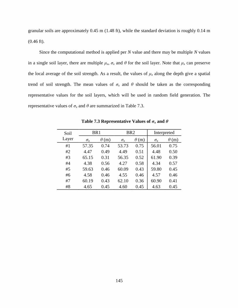
145
granular soils are approximately 0.45 m (1.48 ft), while the standard deviation is roughly 0.14 m
(0.46 ft).
Since the computational method is applied per N value and there may be multiple N values
in a single soil layer, there are multiple μx, ζx and θ for the soil layer. Note that μx can preserve
the local average of the soil strength. As a result, the values of μx along the depth give a spatial
trend of soil strength. The mean values of ζx and θ should be taken as the corresponding
representative values for the soil layers, which will be used in random field generation. The
representative values of ζx and θ are summarized in Table 7.3.
Table 7.3 Representative Values of σx and θ
Soil
Layer
BR1 BR2 Interpreted
ζx θ (m) ζx θ (m) ζx θ (m)
#1 57.35 0.74 53.73 0.75 56.01 0.75
#2 4.47 0.49 4.49 0.51 4.48 0.50
#3 65.15 0.31 56.35 0.52 61.90 0.39
#4 4.38 0.56 4.27 0.58 4.34 0.57
#5 59.63 0.46 60.09 0.43 59.80 0.45
#6 4.58 0.46 4.55 0.46 4.57 0.46
#7 60.19 0.43 62.10 0.36 60.90 0.41
#8 4.65 0.45 4.60 0.45 4.63 0.45

146
Figure 7.6 CDF of correlation length for cohesive soils
Figure 7.7 CDF of correlation length for granular soils
(Note: 0.3 m = 0.98 ft; 0.4 m = 1.31 ft; 0.5 m = 1.64 ft; 0.6 m = 1.97 ft; 0.7 m = 2.3 ft; 0.8 m =
2.62 ft.)
0.2 0.3 0.4 0.5 0.6 0.7 0.8 0.90
0.2
0.4
0.6
0.8
1
Cohesive SoilsSample Size = 18Minimum = 0.288 mMaximum = 0.751 mMean = 0.448 mStandard Deviation = 0.149 m
, m
Cu
mu
lati
ve D
istr
ibu
tio
n F
un
cti
on
0.4 0.5 0.6 0.7 0.80
0.2
0.4
0.6
0.8
1
Granular SoilsSample Size = 27Minimum = 0.312 mMaximum = 0.771 mMean = 0.516 mStandard Deviation = 0.130 m
, m
Cu
mu
lati
ve D
istr
ibu
tio
n F
un
cti
on

147
7.4.3 Determination of Soil Profile for Reliability Analysis
It has been shown in Figure 7.2 that the drilled shaft is not constructed at the locations
where SPT was conducted. As a result, the soil profile at the location where the drilled shaft is
constructed should be determined based on the findings of the subsurface investigation. The
objective of this section is to demonstrate the use of inverse distance method in interpreting the
soil profile given the adjacent boring logs.
In subsurface investigation, the soil samples are retrieved. Hence, the soil stratifications at
the boring locations can be established and the thickness of each soil layer is known. In order to
identify the soil stratifications at the desired location, it is assumed that the same soil
stratifications are still present at that location. However, the thickness of each soil layer may be
different. With this assumption, the thicknesses of the soil layers at the desired location need to
be determined using the inverse distance method, and the distance between two points can be
calculated based on their coordinates. In this example, the distances from the location where the
drilled shaft is constructed to the locations of BR1 and BR2 are 15.6 m (51.18 ft) and 19.3 m
(63.32 ft), respectively. The relative weight for BR1 and BR2 would be 0.63 and 0.37, assuming
a v equal to 2.5 in Equation (7.13b). Figure 7.8 shows the interpreted soil stratifications for the
drilled shaft based on the adjacent borings. It can be seen that the interpreted soil stratifications
are close to those at BR1 and BR2, because the inverse distance method gives a weighted
average based on the adjacent observations. Likewise, the inverse distance method can be
applied to estimate other parameters based on the boring logs of BR1 and BR2. The ―Interpreted‖
column in Table 7.3 summarizes the representative values of ζx and θ at the location where the
drilled shaft is constructed, while Table 7.4 summarizes the spatial trend of the strength
parameter x.

148
Table 7.4 Spatial Trend of Strength Parameter along the Depth
Elevation(m) x μx
253.0 ϕ′ 36.2
251.0 ϕ′ 36.2
251.0 Su 199.5
250.5 Su 199.4
250.0 Su 199.2
248.9 Su 199.0
248.9 ϕ′ 35.8
243.7 ϕ′ 35.8
243.7 Su 271.8
242.9 Su 271.9
242.4 Su 272.0
240.4 Su 272.3
237.8 Su 272.7
237.8 ϕ′ 42.1
235.3 ϕ′ 42.1
234.8 ϕ′ 42.0
230.7 ϕ′ 41.9
227.7 ϕ′ 41.9
Figure 7.8 The interpreted soil stratifications based on adjacent borings
0
5
10
15
20
25
30
35
Dep
th,
m
BR1 BR2 Interpreted
Cohesive
Granular
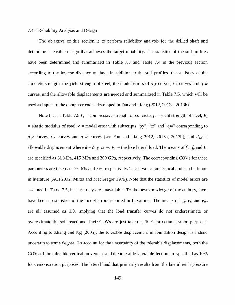
149
7.4.4 Reliability Analysis and Design
The objective of this section is to perform reliability analysis for the drilled shaft and
determine a feasible design that achieves the target reliability. The statistics of the soil profiles
have been determined and summarized in Table 7.3 and Table 7.4 in the previous section
according to the inverse distance method. In addition to the soil profiles, the statistics of the
concrete strength, the yield strength of steel, the model errors of p-y curves, t-z curves and q-w
curves, and the allowable displacements are needed and summarized in Table 7.5, which will be
used as inputs to the computer codes developed in Fan and Liang (2012, 2013a, 2013b).
Note that in Table 7.5 f′c = compressive strength of concrete; fy = yield strength of steel; Es
= elastic modulus of steel; e = model error with subscripts ―py‖, ―tz‖ and ―qw‖ corresponding to
p-y curves, t-z curves and q-w curves (see Fan and Liang 2012, 2013a, 2013b); and da,d =
allowable displacement where d = δ, ψ or w, VL = the live lateral load. The means of f′c, fy and Es
are specified as 31 MPa, 415 MPa and 200 GPa, respectively. The corresponding COVs for these
parameters are taken as 7%, 5% and 5%, respectively. These values are typical and can be found
in literature (ACI 2002; Mirza and MacGregor 1979). Note that the statistics of model errors are
assumed in Table 7.5, because they are unavailable. To the best knowledge of the authors, there
have been no statistics of the model errors reported in literatures. The means of epy, etz and eqw
are all assumed as 1.0, implying that the load transfer curves do not underestimate or
overestimate the soil reactions. Their COVs are just taken as 10% for demonstration purposes.
According to Zhang and Ng (2005), the tolerable displacement in foundation design is indeed
uncertain to some degree. To account for the uncertainty of the tolerable displacements, both the
COVs of the tolerable vertical movement and the tolerable lateral deflection are specified as 10%
for demonstration purposes. The lateral load that primarily results from the lateral earth pressure
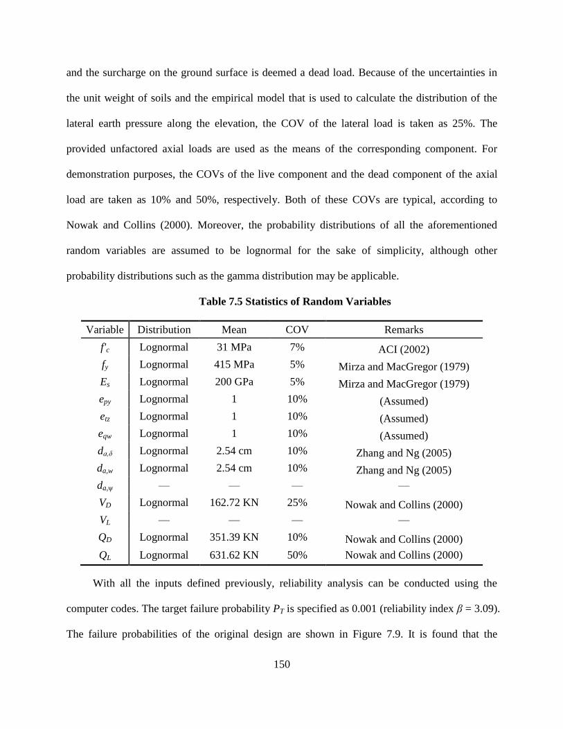
150
and the surcharge on the ground surface is deemed a dead load. Because of the uncertainties in
the unit weight of soils and the empirical model that is used to calculate the distribution of the
lateral earth pressure along the elevation, the COV of the lateral load is taken as 25%. The
provided unfactored axial loads are used as the means of the corresponding component. For
demonstration purposes, the COVs of the live component and the dead component of the axial
load are taken as 10% and 50%, respectively. Both of these COVs are typical, according to
Nowak and Collins (2000). Moreover, the probability distributions of all the aforementioned
random variables are assumed to be lognormal for the sake of simplicity, although other
probability distributions such as the gamma distribution may be applicable.
Table 7.5 Statistics of Random Variables
Variable Distribution Mean COV Remarks
f'c Lognormal 31 MPa 7% ACI (2002)
fy Lognormal 415 MPa 5% Mirza and MacGregor (1979)
Es Lognormal 200 GPa 5% Mirza and MacGregor (1979)
epy Lognormal 1 10% (Assumed)
etz Lognormal 1 10% (Assumed)
eqw Lognormal 1 10% (Assumed)
da,δ Lognormal 2.54 cm 10% Zhang and Ng (2005)
da,w Lognormal 2.54 cm 10% Zhang and Ng (2005)
da,ψ — — — —
VD Lognormal 162.72 KN 25% Nowak and Collins (2000)
VL — — — —
QD Lognormal 351.39 KN 10% Nowak and Collins (2000)
QL Lognormal 631.62 KN 50% Nowak and Collins (2000)
With all the inputs defined previously, reliability analysis can be conducted using the
computer codes. The target failure probability PT is specified as 0.001 (reliability index β = 3.09).
The failure probabilities of the original design are shown in Figure 7.9. It is found that the
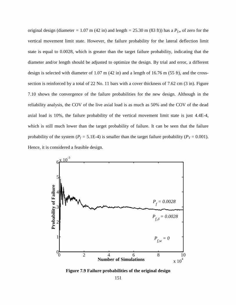
151
original design (diameter = 1.07 m (42 in) and length = 25.30 m (83 ft)) has a Pf,w of zero for the
vertical movement limit state. However, the failure probability for the lateral deflection limit
state is equal to 0.0028, which is greater than the target failure probability, indicating that the
diameter and/or length should be adjusted to optimize the design. By trial and error, a different
design is selected with diameter of 1.07 m (42 in) and a length of 16.76 m (55 ft), and the cross-
section is reinforced by a total of 22 No. 11 bars with a cover thickness of 7.62 cm (3 in). Figure
7.10 shows the convergence of the failure probabilities for the new design. Although in the
reliability analysis, the COV of the live axial load is as much as 50% and the COV of the dead
axial load is 10%, the failure probability of the vertical movement limit state is just 4.4E-4,
which is still much lower than the target probability of failure. It can be seen that the failure
probability of the system (Pf = 5.1E-4) is smaller than the target failure probability (PT = 0.001).
Hence, it is considered a feasible design.
Figure 7.9 Failure probabilities of the original design
0 2 4 6 8 10
x 104
0
1
2
3
4
5
6x 10
-3
Number of Simulations
Pro
ba
bil
ity
of
Fa
ilu
re
Pf = 0.0028
Pf,
= 0.0028
Pf,w
= 0

152
Figure 7.10 Failure probabilities by MCS
The new design by the proposed performance based design approach is compared with the
original design (diameter = 1.07 m (42 in) and length = 25.30 m (83 ft)). First, the diameter of
the new design is the same as that of the original design, and the new design has two more
longitudinal bars than the original design as reinforcements. On the other hand, it is noticeable
that the new design has a much shorter length than the original design: the new design is just 66%
as long as the original design. While the difference in reinforcing rebars between the two designs
is minimal, the difference in the length between the two designs is significant. This finding can
be attributed to the design for the axial loads. Note that the average axial capacity of the original
design in Monte Carlo simulation is 5125.9 KN (1152.30 kips), which is obtained according to
the performance criterion (allowable displacement of 2.54 cm (1 in)). Likewise, the average axial
capacity of the new design is just 3254.6 KN (731.63 kips) using the same performance criterion.
0 2 4 6 8 10
x 104
0
0.5
1
1.5x 10
-3
Number of Simulations
Pro
ba
bil
ity
of
Fa
ilu
re
Pf = 5.1E-4
Pf,
= 7.0E-5
Pf,w
= 4.4E-4
Target

153
Notice that the summation of the unfactored dead load and the unfactored live load is 351.39 +
631.62 = 983.01 KN (220.98 kips). Accordingly, the factor of safety would be 5.215 for the
original design and 3.311 for the new design. There is a significant difference between the
factors of safety.
As indicated by the factors of safety, the original design may be too conservative for the
axial loads. This same conclusion can be reached from the viewpoint of the failure probability.
Notice that failure probability of the vertical movement limit state is zero for the sample size of
100,000, much lower than the target failure probability. In spite of the length of 25.30 m (83 ft),
the system failure probability of the original design is just 0.0028 in relation to the failure
probability of the lateral deflection limit state, indicating that the design is unable to achieve the
target reliability. This is because the transfer of lateral loads occurs primarily in the upper zone
of the drilled shaft and additional length is no longer ineffective in reducing the lateral deflection
at the top of the drilled shaft.
Furthermore, it should be pointed out that the system reliability has been considered in the
new design. As concluded in the Fan and Liang (2013a), the failure probability of the system is
greater than those of the individual failure modes in reliability analysis. In the consideration of
the system reliability, although the new design has slightly bigger diameter and slightly higher
reinforcement ratio, the system failure probability for the new design is just 9.9E-4. From the
viewpoint of the system failure probability, the new design is more reliable than the original
design.
7.5 Summary and Conclusions
The stochastic nature of soil properties plays an important role in reliability-based design
and risk management. This research presents a Bayesian approach that can be applied to
154
characterize the spatial variability of soil properties using SPT data. In order to establish a
probabilistic model for SPT data in the Bayesian approach, it is assumed that the mean, the
standard deviation and the correlation structure in the interval of each N value remain unchanged.
Moreover, it is assumed that the strength parameter such undrained shear strength for cohesive
soils and effective friction angle for granular soil follows lognormal distribution. With the
establishment of the probabilistic model, Markov chain Monte Carlo is implemented to draw
samples of the parameters (μ, ζ, ρ). The resulting samples can be used to estimate (μ, ζ, ρ). The
mean μ measures the center of a dataset, the standard deviation measures the variability of a
random variable while the correlation length measure how rapidly a random field varies in space.
Furthermore, a kriging technique called inverse distance method is presented to interpret the soil
profiles based on adjacent borings. Finally, an example is given and the following conclusions
are made:
1. The computational method can be applied to characterize the spatial variability of soil
properties using SPT data. It is applied per N value. If there are multiple N values in a
single soil layer, then ζx and θ should be averaged, and the average values should be
taken as the representative values for the soil layer.
2. The resulting correlation length in this study is distributed over the range from 0.2 m
(0.66 ft) to 0.8 m (2.62 ft). The corresponding mean is approximately 0.45 m (1.48 ft),
while the standard deviation is about 0.15 m (0.49 ft).
3. The computational method can preserve the local average of the soil properties. The
values of μx along the depth give a spatial trend of the soil strength.

155
4. The inverse distance method provides a simple means to interpret the soil profiles
according to the adjacent borings. In the inverse distance method, more weight is given to
the observations that are close to the desired location.
5. In the example, the feasible design by the performance based design approach is
significantly different from the original design that was obtained using load and
resistance factor design. The factor of safety of the new design is just 3.311. However,
the factor of safety of the original design is as much as 5.215, indicating that the original
design might be too conservative.
156
CHAPTER 8. SUMMARY AND CONCLUSIONS
8.1 Summary of the Research
Reliability-based design of deep foundations, such as drilled shafts and driven piles, has
become increasingly important due to the heightened awareness of the shortcomings of the
conventional allowable stress design approach. For example, the load and resistance factor
design has been implemented by American Association of State Highway Transportation
Officials (AASHTO) since 2007. Nevertheless, there are still many unsolved issues regarding the
implementation of load and resistance factor design. For example, there is no generally accepted
guidance on the statistical characterization of soil properties. Moreover, the serviceability limit
check in LRFD is still deterministic. No uncertainties arising in soil properties, loads and design
criteria are taken into account in the current version of LRFD for the serviceability limit check.
In current practice, the load factors and resistances are taken as unity and deterministic models
are applied to evaluate the displacements of geotechnical structures.
In order to address the aforementioned issues of LRFD, the computational method for
conducting reliability analysis and the computational tools for statistically characterizing the
variability of soil properties are needed. The main objectives of the research are:
1. To develop mathematically sound computational tools for conducting reliability
analysis for deep foundations; and
2. To develop the associated computational method that can be used to determine the
variability model of soil properties.

157
In this research, to achieve a consistency between the strength limit check and the
serviceability limit check of the LRFD framework, performance-based design methodology was
developed for deep foundation design. In the proposed methodology, the design criteria are
defined in terms of the displacements of the structure that are induced by external loads. If the
displacements are within the specified design criteria (i.e., the allowable displacement of the
foundation system), the design is considered satisfactory. Otherwise, failure is said to occur. To
calculate the probability of failure, Monte Carlo simulation is employed. In Monte Carlo
simulation, the variability of the random variables that are involved in the reliability analysis is
captured by simulating a large number of the samples according to their respective probability
distributions. Then the simulations of the random variables are used as the input to the
commonly-used deterministic numerical algorithms including the p-y method for lateral load and
the t-z model for axial load to evaluate the load-displacement behavior. With the calculated
displacements, it can be determined whether or not failure occurs. Accordingly, the failure
probability is calculated as the number of failure events to the total number of simulations.
8.1.1 Computational Tools for Reliability Analysis
A series of computer codes have been developed to facilitate the computation of reliability
analysis. Specifically, P-LPILE has been developed for laterally loaded drilled shafts, P-TZPILE
has been developed for axially loaded piles, and XPILE has been developed for piles under
combined axial and lateral loads. Furthermore, a computer code based on importance sampling
has been developed for axially loaded piles in order to have a faster rate of convergence in
estimating the failure probability.
Various sources of uncertainties are accounted for in the proposed reliability methodology.
In all the aforementioned computer codes, the soil properties are modeled as random fields that

158
are statistically characterized by the mean, the standard deviation and the correlation length. The
mean measures the center of a dataset, the standard deviation measures the variability of a
random variable, and the correlation length measures how rapidly a random field varies in space.
The probability distribution of the soil properties is assumed to be lognormal, just for
mathematical simplicity and the ease of simulation. In addition to the variability of soil
properties, the variability of the external loads, concrete properties, steel properties, the design
criteria and the model uncertainty of the load transfer curves can be systematically taken into
account.
Extensive validations were carried out to ensure accuracy and robustness of the developed
computer codes. Furthermore, these computer codes were used for conducting a series of
parametric studies as well as performing several illustrative design examples.
8.1.2 Computational Method for Determining Soil Variability
The method of determining the relevant variability model for soil properties based on the
standard penetration test (SPT) data was developed. The computational method is based on
Bayesian approach. To make the computational method usable to practicing engineers, data from
the SPT is used in the computational method. The objective of developing the method is to
determine the required input including the mean μ, standard deviation ζ, and correlation length θ
of soil properties in reliability analysis and foundation analysis. Several assumptions are invoked
in formulating the approach: 1) each N value in SPT is considered as a unit in the computation; 2)
the mean, standard deviation and the correlation structure of soil properties remain unchanged in
the interval of each N value; and 3) soil properties follow lognormal distributions. In Bayesian
approach, the parameters of interest are λ = (μ, ζ, θ). With these assumptions, the probabilistic
model of the blow counts in SPT can be established as multivariate normal distribution.

159
Accordingly, the posterior distribution of λ can be formulated. Markov chain Monte Carlo is
implemented to draw the samples of (μ, ζ, θ). The advantages of implementing Markov chain
Monte Carlo are that: 1) the normalizing constant in the posterior distribution of the parameters
can be avoided; and 2) it is straightforward to use the resulting samples of the parameters (μ, ζ, θ)
to conduct statistical analysis. An example was given to demonstrate the application of the
proposed site variability characterization method. In addition, the design based on the proposed
reliability method is compared with that based on the current LRFD approach. The comparison
indicates that the current LRFD method yields a very conservative design.
8.2 Conclusions
Using the developed computer codes and the computational method, a series of parametric
studies are conducted. Furthermore, to demonstrate the application of the proposed methodology,
real data from a construction project is used, and the proposed computational method is
employed to determine the variability of the soil properties. Next, the determined variability
model of soil properties is used as input to the developed computer codes in the reliability
analysis. Based on the results of parametric studies and the reliability analysis, the following
conclusions are made:
Reliability Analysis Of Piles Under Axial And Lateral Loads
1. The spatial variability of soil properties, particularly the COV and correlation length of
undrained shear strength for cohesive soils, could exert significant influences on the
computed probability of failure for the specified performance criteria. The difference in
the computed probability of failure caused by different correlation length of Su could be
several orders of magnitude.

160
2. Apart from soil spatial variability, the proposed performance based design approach
provides a systematic procedure to consider uncertainties of the computational model
and the applied loads. A random bias factor is introduced to account for the uncertainty
of p-y curves. The estimated probability of failure increases if the uncertainty of the
adopted p-y curves is considered. The uncertainty of loads is considered by sampling
from their probability distributions and using the samples as input. The calculated
probability of failure increases when the uncertainty of loads is considered.
3. The proposed approach is useful to conduct reliability analysis for serviceability limit
check in the current LRFD framework. Based on the conducted parametric studies, the
reliability for the serviceability limit design of a laterally loaded pile is sensitive to the
spatial correlation of soil properties, soil variability, uncertainty of p-y curves and
loads.
4. The proposed approach is very versatile, as it allows practicing engineers to input the
means, variances and probability distributions of the load model, soil properties and the
bias factor of p-y curves. Furthermore, they can specify the target reliability index
according to the intended functions of the structures under consideration.
5. Probabilistic approaches that do not take into consideration of spatial variance of soil
properties may potentially result in a foundation design that would not meet the
performance criteria with the target reliability. It is demonstrated that the probability of
failure is sensitive to correlation length, θ. If θ is not considered in reliability
assessment, the estimated probability of failure would probably be biased. Therefore,
considering correlation length is warranted in the reliability analysis of deep

161
foundations. There is a strong incentive to use a reliability method that considers the
correlation structure of soil properties for deep foundations.
The Importance Sampling Technique
6. The proposed importance sampling method gives the same unbiased estimate of the
failure probability as the crude MCS method. Nevertheless, the proposed importance
sampling method is much more efficient than the crude MCS method when evaluating
a small Pf (e.g., Pf ≤ 1/1000). By drawing more samples from the region of interest, the
proposed method will achieve a faster rate of convergence. With the same sample size,
the estimate obtained by using the importance sampling method would have a much
smaller coefficient of variation than the estimate obtained by the crude MCS method. It
is recommended to use the importance sampling method in the evaluation of small Pf.
7. The probability of failure evaluated by the commonly used FORM may significantly
deviate from those of Monte Carlo statistical methods, although the reliability index by
FORM is close to those of Monte Carlo statistical methods. The differences in the
failure probabilities between FORM and Monte Carlo statistical methods are primarily
attributed to the approximation of the limit state function in the response surface
method and the linear truncation of the limit state function in the FORM.
The Analysis Of The System Reliability
8. The failure probability of the system, Pf, is greater than any of the three component
failure modes. In addition, Pf is less than the summation of the failure probabilities of

162
the three component failure modes. The failure probability of the system may be
underestimated if multiple failure modes are not considered simultaneously.
9. It is recommended to use the system reliability if multiple failure modes exist. In the
current LRFD approach, different limit states are considered separately, which leads to
overestimation in the reliability.
The Importance Analysis Of Random Variables
10. The importance analysis of the random variables indicate that the major sources of
uncertainties affecting the reliability of a designed drilled shaft come from external
loads, the allowable displacement, soil property Su, and the model factors of the load
transfer curves. The variability in concrete and reinforcement is relatively less
important.
Site Variability Characterization
11. A computational method has been developed that can be applied to characterize the
spatial variability of soil properties using SPT data. It is applied per N value. If there
are multiple N values in a single soil layer, then ζx and θ should be averaged and the
average values should be taken as the representative values for the soil layer.
12. The resulting correlation length in this study is distributed over the range from 0.2 m to
0.8 m. The corresponding mean is approximately 0.45 m while the standard deviation
is about 0.15 m.

163
13. The computational method can preserve the local average of the soil properties. The
values of μx along the depth give a spatial trend of soil strength.
14. The inverse distance method provides a simple means to interpret the soil profiles
according to the adjacent borings. In the inverse distance method, more weights are
given to the observations that are close to the desired location.
15. In the example given in Chapter 7, the feasible design by the performance based design
approach is significantly different from the original design that was obtained using load
and resistance factor design. The factor of safety of the new design is just 3.513.
However, the factor of safety of the original design is as much as 5.215, indicating that
the original design might be too conservative.
8.3 Recommendations for Future Research
Although the computer codes have been developed for conducting reliability analysis and
the computational method has been proposed to determine the variability model for soil
properties, there is a need to continue the current research on the following aspects:
1. To provide statistical guidance to determine the variability of external loads. In the
importance analysis, although the COV of external loads is small, it is noticeable that
the reliability of a design is very sensitive to the external loads. The failure probability
can vary significantly when the COVs of the external loads changes.
2. To calibrate the model uncertainty of the load transfer curves (p-y curves, t-z curves
and q-w curves). Even though the COVs of the load transfer curves are small in the
importance analysis, it can have a big impact on the reliability of a design.
3. To compile a database of the tolerable displacements of deep foundations. The
displacements of interest include lateral deflection, angular distortion and vertical

164
movement. This is because the design criteria are defined by the displacements and it
directly influences the final design. If specified tolerable displacements are too small, it
may lead to conservative designs. Otherwise, unconservative designs will be obtained.
4. To develop a computer code that can be used to conduct reliability analysis on a group
of piles. The computer codes developed in the research only apply to a single drilled
shaft. However, drilled shafts are often constructed as a group. Therefore, it is highly
desirable to develop a computer program for a group of drilled shafts such that the
group effect can be considered in reliability analysis.
5. To continue the research on the effects of the spatial variability on the reliability of the
designed structures and the use of kriging techniques to estimate unknown parameters.

165
REFERENCES
Allen, T. M., Nowak, A. S. and Bathurst, R. (2005) Calibration to Determine Load and
Resistance factors for Geotechnical and Structural Design. No. E-C079, Transportation
Research Board, Washington, D.C.
American Association of State Highway and Transportation Officials (AASHTO). (2010).
AASHTO LRFD Bridge Design Specifications, 5th Edition. American Association of State
Highway and Transportation OfficialsWashington, DC.
American Concrete Institute. (2002). Evaluation of Strength Test Results of Concrete. ACI 214-
R2. American Concrete Institute , Farmington Hills, Michigan.
Ang, A. H-S., and Tang, W. H. (1984). Probability Concepts in Engineering Planning and
Design, Vol. II.. Hoboken, New Jersey: John Wiley and Sons.
Ang, A. H-S., and Tang, W. H. (2007). Probability Concepts in Engineering: Emphasis on
Applications in Civil and Environmental Engineering. Hoboken, New Jersey: John Wiley
and Sons.
Au, S. K., and Beck, J. L. (2003). ―Importance sampling in high dimensions.‖ Structural Safety,
No. 25, 139-163.
Au, S.K, and Beck, J.L. (1999). ―A new adaptive importance sampling scheme for reliability
calculations.‖ Struct. Safety 21: 135-158.

166
Brown, D. A., Turner, J. P., and Casetelli, R. J. (2010). ―Drilled shaft: construction procedures
and LRFD design methods.‖ No. FHWA-NHI-10-016, Federal Highway Administration,
Washington, D.C.
Ching, J. Y., and Phoon, K. K. (2011). ―A quantile-based approach for calibrating reliability-
based partial factors.‖ Structural Safety, 33(2011): 275-285.
Ching, J.Y., Phoon, K.K., Chen, J.R., and Park, J.H. (2013). ―Robustness of constant load and
resistance factors for drilled shafts in multiple strata.‖ J. Geotech. Geoenviron. Engr.,
ASCE, Vol.139(7):1104-1114.
Coyle, H. M., and Reese, L. C. (1966). ―Load transfer for axially loaded piles in clay.‖ Journal
of Soil Mechanics and Foundation Division, 92(2): 1-26.
D’Andrea, A., and Tsai, C. N. (2009). ―Louisiana Department of Transportation’s experience
with LRFD.‖ Implementation status of geotechnical load and resistance factor design in
state department of transportation, No. E-C136, pp. 1-10.
Das, B. (2011). Principles of Foundation Engineering. Stamford, Connecticut: Cengage
Learning. pp. 84-88.
Der Kiureghian, A., and Ke, J.-B. (1995). ―Finite-element based reliability analysis of frame
structures.‖ Proc., ICOSSAR ’85, 4th Int. Conf. on Structural Safety and Reliability,
IASSAR, New York, 1, 395–404.)
Der Kiureghian, A., and Liu, P. L. (1991). ―Optimization algorithms for structural safety.‖ Struct.
Safety, 9:161-177.
Der Kiureghian, A., and Stefano, M. D. (1991). ―Efficient algorithm for second-order reliability
analysis.‖ J. Engr. Mech., 117(12): 2904-2922.
Ditlevsen, O., and Madsen, H.O. (1996). Structural reliability methods. Chichester, UK: Wiley..
167
Ellingwood, B., and Tekie, P. B. (1999). ―Wind load statistics for probability-based structural
design.‖ J. Struct. Eng., 125 (4), 453-463.
Ellingwood, B., Galambos, T. V., MacGregor, J. G., and Cornell, C. A. (1980). Development of a
Probability Based Load Criterion for American National Standard A58. NBS Special
Publication 577. Washington, D.C.: National Bureau of Standards.
Fan, H. J., and Liang, R. (2012). ―Reliability-Based Design of Axially Loaded Drilled Shafts
using Monte Carlo Method.‖ Int. J. of Num. and Analyt. Methods in Geomech. (In Press).
Fan, H. J., and Liang, R. (2013a). ―Probabilistic framework of drilled shaft design considering
soil spatial variability.‖ Journal of the Transportation Research Board. (In Press)
Fan, H. J., and Liang, R. (2013b). ―Performance-Based Reliability Analysis of Laterally Loaded
Drilled Shafts.‖ Journal of Geotechnical and Geoenvironmental Engineering, ASCE.
http://dx.doi.org/10.1061/(ASCE)GT.1943-5606.0000954 (In Press)
Fenton, G. (1999). ―Random field modeling of CPT data.‖ Journal of Geotechnical and
Geoenvironmental Engineering, ASCE, 125 (6), 486-498.
Fenton, G. A., and Griffiths, D. V. (2008). Risk Assessment in Geotechnical Engineering,
Hoboken, New Jersey: Wiley and Sons.
Fishman, G. S. (1996). Monte Carlo: Concepts, Algorithms and Applications. New York:
Springer
Griffiths, D. V., Huang, J., and Fenton, G. (2009). ―Influence of spatially variability on slope
reliability using 2-D random fields.‖ J. Geotech. Geoenviron. Eng., ASCE, 135 (10), 1367-
1378.
Isaaks, E. H., and Srivastava, R. M. (1989) Introduction to Applied Geostatistics. Oxford
University Press, Inc., New York, pp. 249-277.

168
Klammler, H., McVay, M., Horhota, D., and Lai, P. (2010). ―Influence of spatially variable side
friction on single drilled shaft resistance and LRFD resistance factors.‖ J. Geotech.
Geoenviron. Eng., ASCE, 136 (8), 1114-1122.
Kung, G. T. C., Juang, C., Hsein, H., Evan, C. L., and Hashash, Y. M. A. (2007). ―Simplified
model for wall deflection and ground-surface settlement caused by braced excavation in
clays.‖ Journal of Geotechnical and Geoenvironmental Engineering, 133(6): 731-747.
Lai, P. W. (2009). ―Florida Department of Transportation’s experience with LRFD.‖ In:
Implementation Status of Geotechnical Load and Resistance Factor Design in State
Departments of Transportation, Transportation Research Circular No. E-C136, 11-20.
Transportation Research Board, Washington, D.C.
Lee, I. K., White, W., and Ingles, O. G. (1983). Geotechnical Engineering. Melbourne, Australia:
Sir Isaac Pitman and Sons. p. 62
Low, B.K., and Tang, W.H. (2007). ―Efficient spreadsheet algorithm for first order reliability
method.‖ J. Engr. Mech. 133(12): 1378-1387.
Luo, Z., Atamturktur, S., Cai, Y. and Juang, C. H. (2012). ―Simplified approach for reliability-
based design against basal heave failure in braced excavations considering spatial effect.‖ J.
Geotech. Geoenviron. Eng., 128(4), 441-450.
Melchers, R. (1999). Structural Reliability Analysis and Prediction. London: John Wiley and
Sons, Ltd.
Mirza, S.A., and MacGregor, J.G., ―Variability of Mechanical Properties of Reinforcing Bars.‖
Journal of the Structural Division, ASCE. Vol. 105, No. ST5, 1979, pp. 921-937.
Nowak, A. S., and Collins, K. R. (2000). Reliability of structures. New York: McGraw-Hill.
169
Paice, G. M., Griffiths, D. V., and Fenton, G. A. (1996). ―Finite element modeling of settlements
on spatially random soil.‖ J. Geotech. Eng., ASCE, 122(9), 777-779.
Phoon, K. K, Kulhawy, F. H., and Grigoriu, M. D. (1995). ―Reliability-based design of
foundations for transmission line structures.‖ Rep. TR-105000, Electric Power Research
Institute, Palo Alto, California.
Phoon, K. K, Kulhawy, F. H., and Grigoriu, M. D. (2003a). ―Development of a reliability-based
design framework for transmission line structure foundations.‖ J. Geotech. Geoenviron.
Eng., ASCE, 129 (9), 798-806.
Phoon, K. K, Kulhawy, F. H., and Grigoriu, M. D. (2003b). ―Multiple resistance factor design
for shallow transmission line structure foundations.‖ J. Geotech. Geoenviron. Eng., ASCE,
129 (9), 807-818.
Phoon, K. K., and Kulhawy, F. H. (1999). ―Characterization of geotechnical variability.‖ Can.
Geotech. J., Vol. 36, 612-624.
Phoon, K. K., and Kulhawy, F. H. (2005). ―Characterization of model uncertainties for laterally
loaded rigid drilled shafts.‖ Geotechnique, Vol. 55(1), 45-54.
Reese, L. C. (1977). ―Laterally loaded piles: program documentation.‖ J. Geotech. Eng.
Division., Vol. 103 (GT4), ASCE, 287-305.
Reese, L. C., Wang, S. T, and Isenhower, W. M., and Arrellaga, J. A. (2004). Computer program
LPILE Plus version 5.0 technical manual. Austin, Texas: Ensoft. Inc.
Robert, C. P., and Casella, G. (2004). Monte Carlo Statistical Methods, Springer, New York.
Roberts, L. A., and Misra, A. (2010). ―Performance-based design of deep foundation systems in
load and resistance factor design framework.‖ Journal of the Transportation Research
Board, No. 2186, 29-37.

170
Sabatini, P. J., Bachus, R. C, Mayne, P. W., Schneider, J. A., and Zettler, T. E. (2002).
Evaluation of Soil and Rock Properties. Report No. FHWA-IF-02-034. Federal Highway
Administration, Washington, D.C..
Vanmarcke, E. H. (1977). ―Probabilistic modeling of soil profiles.‖ Journal of the Geotechnical
Engineering Division, 103(11), 1227-1246.
Wang, Y., Au, S. K., and Kulhawy, F. H. (2011). ―Expanded reliability-based design approach
for drilled shafts.‖ J. Geotech. Geoenviron. Eng., 137(2), 140-149.
Zhang, L. M., and Ng, Agnes, M. Y. (2005). ―Probabilistic limiting tolerable displacements for
serviceability limit state design of foundations.‖ Geotechnique, 55(2), 151-161.
Zhu, H., and Chang, M. F. (2002). ―Load transfer curves along bored piles considering modulus
degradation.‖ Journal of Geotechnical and Geoenvironmental Engineering 2002, ASCE,
128 (9): 764-773.