Embed Size (px)
Citation preview
PERFORMANCE ANALYSIS OF OPERATING WIND FARMS
Dissertation in partial fulfillment of the requirements for the degree of
MASTER OF SCIENCE WITH A MAJOR IN WIND POWER
PROJECT MANAGEMENT
Uppsala University
Department of Earth Sciences, Campus Gotland
Abdul Mouez Khatab
September 2017
PERFORMANCE ANALYSIS OF OPERATING WIND FARMS
Dissertation in partial fulfillment of the requirements for the degree of
MASTER OF SCIENCE WITH A MAJOR IN WIND POWER
PROJECT MANAGEMENT
Uppsala University
Department of Earth Sciences, Campus Gotland
Approved by:
Supervisor, Hugo Olivares Espinosa
Examiner, Jens Nørkær Sørensen
September 2017
ABSTRACT II
Abdul Mouez Khatab Performance Analysis of Operating Wind Farms
ABSTRACT
Nowadays, wind power is the fastest growing source of energy all around the
world. This poses an urgent need of understanding how wind turbines perform from
different perspectives. Even though condition monitoring systems have a huge impact in
optimizing wind farms performance via fault anticipation, it does omit several aspects
concerning performance. Seemingly, there is a scarcity of studies which attempted to
deliver a quick and practical method for wind farm performance analysis which is the aim
of this master thesis.
This work proposes a methodology to evaluate the performance of operating wind
farms via the use of Supervisory Control and Data Acquisition System (SCADA) and
modeled data. The potential annual energy is calculated per individual turbine considering
underperforming/loss events to have their power output in accordance with a
representative derived operational power curve. Losses/underperformance events are
calculated and categorized into several groups aiming at identifying and quantify their
causes. The methodology requires both anemometry data from SCADA system as well as
modeled data. The discrepancy of the data representing the valid points of the power curve
is taken into consideration as well when assessing the performance, i.e. wind speed vs
power output of events that are not loss/underperformance. Production loss and relative
standard deviation of power output of what is defined as “valid sample” in this work (per
each turbine) are the main results obtained in this work. Finally, a number of optimization
measures are suggested in order to enhance the performance, which can lead to a boost in
the financial output of a wind farm.
Aiming at judging the reliability of the proposed methodology, a case study is
conducted and evaluated. The investigated case study shows that the methodology is
capable of determining potential energy and associated losses/underperformance events.
Several questions were raised during the assessment and are discussed in this report,

ABSTRACT III
Abdul Mouez Khatab Performance Analysis of Operating Wind Farms
recommendation for optimization measures are presented at the end of the study. Also, a
discussion on the limitations and uncertainties associated to the presented methodology
and the case study.

ACKNOWLEDGEMENTS IV
Abdul Mouez Khatab Performance Analysis of Operating Wind Farms
ACKNOWLEDGEMENTS
First and foremost, I would like to express my deepest gratitude for Hugo Olivares for his guidance and advice through the course of this work. I would like as well to thank the staff of the wind power department for the great notion they have passed to us. Many thanks and hugs to wind power project management students. Especially those who I shared special moments with. You have a huge impact on my life guys Philippo, Esmy, Andis, Piia, Jose, Marc and Sören. I would also like to thank Geoffry for his time and efforts reviewing this report. I cannot but seize the opportunity to tell my lovely Raya that I adore her and that I am so proud of us. I cannot wait until we start our own journey together <3 Family and friends who are close or faraway due to unforeseen circumstances. I really wish you were here to share this moment with me. You mean the world for me. To everyone who has contributed to where I am today. Whether we were close or not. Thanks for everything.
NOMENCLATURE V
Abdul Mouez Khatab Performance Analysis of Operating Wind Farms
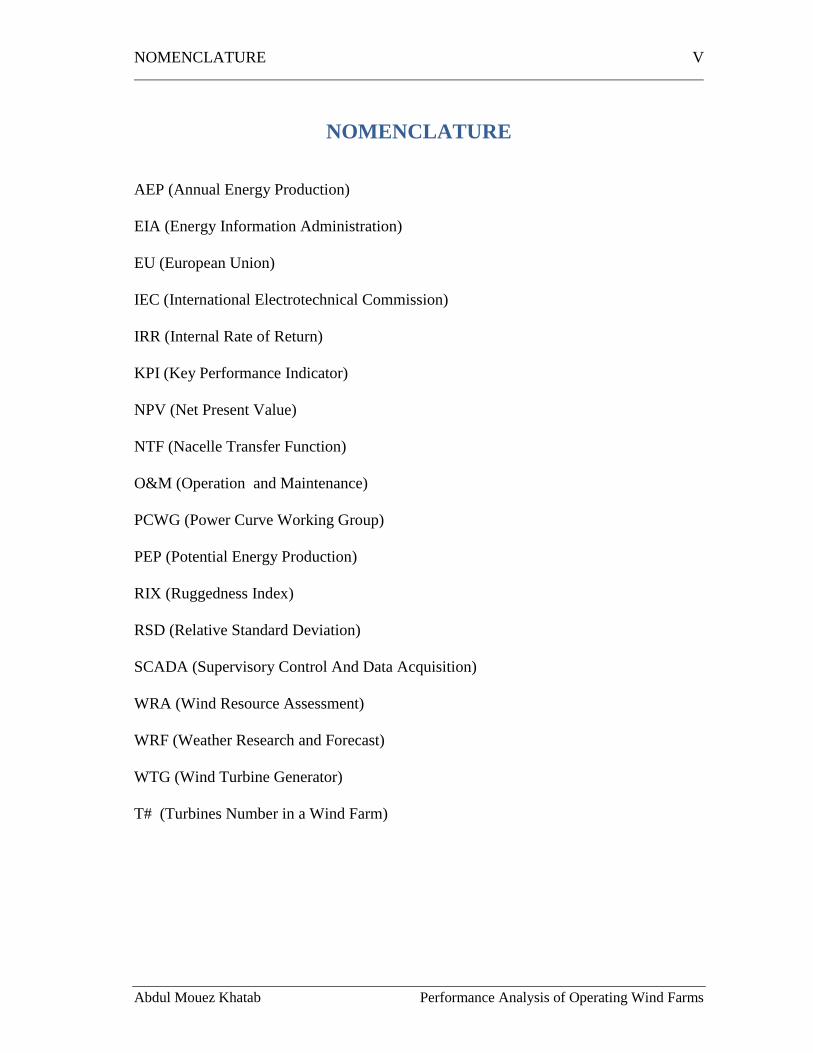
NOMENCLATURE
AEP (Annual Energy Production)
EIA (Energy Information Administration)
EU (European Union)
IEC (International Electrotechnical Commission)
IRR (Internal Rate of Return)
KPI (Key Performance Indicator)
NPV (Net Present Value)
NTF (Nacelle Transfer Function)
O&M (Operation and Maintenance)
PCWG (Power Curve Working Group)
PEP (Potential Energy Production)
RIX (Ruggedness Index)
RSD (Relative Standard Deviation)
SCADA (Supervisory Control And Data Acquisition)
WRA (Wind Resource Assessment)
WRF (Weather Research and Forecast)
WTG (Wind Turbine Generator)
T# (Turbines Number in a Wind Farm)
TABLE OF CONTENTS VI
Abdul Mouez Khatab Performance Analysis of Operating Wind Farms
TABLE OF CONTENTS ABSTRACT ...................................................................................................................... II
ACKNOWLEDGEMENTS .............................................................................................IV
NOMENCLATURE .......................................................................................................... V
LIST OF FIGURES ....................................................................................................... VIII
LIST OF TABLES ............................................................................................................ X
1. INTRODUCTION ...................................................................................................... 1
1.1. Background .......................................................................................................... 1
1.2. Important Definitions .......................................................................................... 1
1.3. Objective and Research Questions ...................................................................... 3
1.4. Justification of the Research ................................................................................ 4
1.5. Methodology ........................................................................................................ 4
1.6. Outline ................................................................................................................. 4
2. LITERATURE REVIEW ........................................................................................... 6
2.1. Introduction ......................................................................................................... 6
2.2. Performance Analysis .......................................................................................... 6
2.2.1. Power Performance Test .............................................................................. 6
2.2.2. Directional Behavior .................................................................................. 11
2.2.3. Pitch Mechanism ........................................................................................ 12
2.3. Utilization of SCADA System in Loss/Underperformance Assessment ........... 12
2.3.1. Loss Assessment ........................................................................................ 12
2.3.2. Down time Analysis ................................................................................... 19
2.3.3. Icing Detection and Quantification ............................................................ 22
2.4. Reasons for Performance Deviation .................................................................. 26
2.4.1. Pre-construction uncertainties .................................................................... 27
2.4.2. Underperformance causes .......................................................................... 29
2.4.3. Production loss detection and quantification ............................................. 30
2.5. Optimization Measures ...................................................................................... 31
2.5.1. Hardware Installation ................................................................................. 31
2.5.2. Parametric Adjustment ............................................................................... 35
TABLE OF CONTENTS VII
Abdul Mouez Khatab Performance Analysis of Operating Wind Farms
2.6. Conclusions of Literature Review ..................................................................... 36
3. METHODOLOGY ................................................................................................... 38
4. RESULTS, DISCUSSION, AND ANALYSIS ........................................................ 44
4.1. Case study Description ...................................................................................... 44
4.2. Filtration and Operational Power Curve Creation ............................................. 44
4.3. Faulty Logs Replacement .................................................................................. 48
4.4. Production Loss ................................................................................................. 52
4.5. Loss Categories and Underperformance ............................................................ 53
4.6. Discrepancy Analysis ........................................................................................ 56
4.7. Optimization Measures ...................................................................................... 58
5. CONCLUSIONS ...................................................................................................... 59
5.1. Summary of the Work ....................................................................................... 59
5.2. Limitations ......................................................................................................... 59
5.3. Future Work ....................................................................................................... 60
REFERENCES ................................................................................................................. 61
APPENDECIES ............................................................................................................... 63
APPENDIX A. LOSS CATEGORIES PER TURBINE AND YEAR ........................ 63
APPENDIX B. VALID SAMPLE DISCREPANCY .................................................. 65
APPENDIX C. PROBABILITY AND PERCENTAGE OF PRODUCTION LOSS
PER CHOSEN CATEGORIES. ................................................................................... 67
APPENDIX D. RESULTS PER TURBINE AND YEAR ........................................... 69
LIST OF FIGURES VIII
Abdul Mouez Khatab Performance Analysis of Operating Wind Farms
LIST OF FIGURES
Figure 1: Example of wind turbine power curve provided by the manufacturer. (“ERU
Met Data - Wind Turbine Power,” 2017) ........................................................................... 3
Figure 2: Power Performance Test Methodology in Accordance with the IEC Standard
IEC 61400-12-2. (International Electrotechnical Commission, 2013)............................... 7 Figure 3: Deviation between measured and guaranteed power curves. (Oh and Kim,
2015). .................................................................................................................................. 9 Figure 4: Health indices based on the power curves. The difference between the
warranted power curve (grey) and the measured power curve (dashed black) can be
defined by the distance between both curves (solid black) or by the ratio of the area
under the measured power curve (green and blue) and the area under the warranted
power curve (blue). (Nymfa Noppe, 2014). ..................................................................... 10 Figure 5: Energy ratio for a selection of turbines in a given wind farm. Source: (Singh,
2013). ................................................................................................................................ 14
Figure 6: Example of power ratio matrix for a given wind farm with 11 turbines. Source:
(Lindvall et al., 2016). ...................................................................................................... 17 Figure 7: Contribution to turbine down time by turbine for a given wind farm of 60
turbines where red, green and blue bars represent contribution to number of events,
duration of events, and duration between events respectively. Source: (Singh, 2013). ... 21
Figure 8: Contribution to turbine down time per category for a given wind farm of 60
turbines. Source: (Singh, 2013). ....................................................................................... 22 Figure 9: Threshold icing methodologies; Wind speed vs power (top row), wind speed vs
power difference (bottom row). The three different columns represent methods of
calculating icing threshold, flat percentage (perc), quantile (quant) and standard
deviation (sd). Source: (Davis et al., 2015). ..................................................................... 24 Figure 10: Median power curve (P50), threshold power curve used for detection of ice
(P10) and data flagged as iced during March 2013 for a given wind turbine. Source:
(Hansson et al., 2016). ...................................................................................................... 25
Figure 11: The estimated energy loss due to icing for a given wind farm, based on
operational data (threshold power curve) and modeled data. Numbers above the bars are
production index that provides information about the production each year with respect
to the average of all years (index 100). Source: (Hansson et al., 2016). .......................... 26 Figure 12: wind conditions and power curve. Source: (Turkyilmaz et al., 2016). ........... 28
Figure 13: Failure/Turbine/year and down time for two large surveys of onshore
European wind turbines over 13 years. Source: (Sheng, 2013). ...................................... 30
Figure 14: Contributors to component failure. Source: (Sheng, 2013). ........................... 31 Figure 15: Steps of the effective condition monitoring process. Source: (Morton, 2013).
.......................................................................................................................................... 32 Figure 16: Flow chart of the proposed methodology. ...................................................... 38 Figure 17: Wind rose of the studied wind farm based on 16 years modeled data. .......... 44
Figure 18: Using calculated average and standard deviation power values for the range
beyond the rated power may mark losses as valid points due to a low number of records
per bin. .............................................................................................................................. 46
LIST OF FIGURES IX
Abdul Mouez Khatab Performance Analysis of Operating Wind Farms
Figure 19: Delineation of the operational power curve. ................................................... 47 Figure 20: The valid sample (points which considered to have actual power output as
expected). ......................................................................................................................... 48 Figure 21: Data compensation quality for T04 in 2013. .................................................. 50
Figure 22: Data compensation quality of T04 in 2014. .................................................... 50 Figure 23: Data compensation quality of T04 in 2015. .................................................... 51 Figure 24: Data compensation quality of T04 in 2016. .................................................... 51 Figure 25: Production Loss Summary for the studied wind farm. ................................... 52 Figure 26: Production loss of each wind turbine in 2014 divided into different categories
.......................................................................................................................................... 54 Figure 27: Monthly data of the entire wind farm in 2014. ............................................... 56
Figure 28: Relative Standard Deviation of power values (data discrepancy) of valid
samples of all turbines in 2014. ........................................................................................ 57
LIST OF TABLES X
Abdul Mouez Khatab Performance Analysis of Operating Wind Farms
LIST OF TABLES
Table 1: Calculated AEP values and relative errors using measured and guaranteed
power curves. Source: (Oh and Kim, 2015) ...................................................................... 9 Table 2: Summary of the main characteristics of the potential energy production
methods. Source: (Lindvall et al., 2016). ......................................................................... 15
Table 3: Group of representative WTGs for a given wind farm of 11 turbines. Source:
(Lindvall et al., 2016). ...................................................................................................... 18 Table 4: Neighboring ranking based on smallest bias and west-southwesterly wind
direction for a given wind farm of 11 turbines. Source: (Lindvall et al., 2016). ............. 19 Table 5: The methodologies suggested by Davis et al. (2015) for icing loss calculation.
Source: (Davis et al., 2015). ............................................................................................. 23 Table 6: Summary of the results obtained concerning the yaw alignment analysis of a
given wind turbine. ........................................................................................................... 34 Table 7: Energy production, losses, and gains during icing with anti/deicing-icing system
installed. Source: (Klemm, 2014). ................................................................................... 34 Table 8: Schedule for an operating wind farm consisting of five wind turbines for the
next 12-time points where si indicates whether the turbine should be operating (1) or not
(0). τi is the normalized generator torque between 0-100. ßi is the normalized blade pitch
angle between -0.57° and 90°. Source: (Zhang, 2012). .................................................... 36
Table 9: Relative Standard Deviation after filtration (valid sample) for T02 in 2014. .... 45 Table 10:Modeled WRF data characteristics. ................................................................ 48
Table 11: SCADA system functionality of the given wind farm. .................................... 49
Table 12: Occurrence frequency of the losses different categories for the period 2013-
2016. ................................................................................................................................. 53 Table 13: Probability and percentage of production loss per chosen categories in 2014. 55
INTRODUCTION 1
Abdul Mouez Khatab Performance Analysis of Operating Wind Farms
1. INTRODUCTION
1.1. Background
Climate change has been a priority for the global collaboration. It has required a
lot of international attention and efforts recently in order to keep the Earth within the
+2°C above what it was before the industrialization period. It has even been set among
the Sustainable Development Goals of the United Nations (United Nations, 2015).
According to the Environmental Protection Agency in the United States, the energy and
heating sector was responsible for the highest share of the global greenhouse gas
emissions in 2010 with 25% of the total emissions (Boden et al., 2017). Therefore, a
pioneered transition toward a cleaner energy system is needed. Among the various clean
energy sources, wind power has emerged as the fastest growing energy source in the
world (Dye, 2016). This poses an urgent need to minimize the levelized costs of energy
and enhance asset management mechanisms. Accordingly, it is of great importance to
come up with various optimization techniques to maintain the prices in a range that
guarantees this fast growth, especially with the witnessed trend in utilizing tenders and
market-based support systems in most of the European Union (EU) countries (ECOFYS,
2014).
1.2. Important Definitions
A number of terminology is crucial for the reader in order to benefit from the proposed
methodology and the presented results in this work. Three important concepts are:
“Acronym for supervisory control and data acquisition, a computer system for gathering
and analyzing real time data. SCADA systems are used to monitor and control a plant or
equipment in industries such as telecommunications, water and waste control, energy, oil
and gas refining and transportation” (“What is SCADA? Webopedia Definition,” 2017).
In wind power regards, a SCADA system gathers information, such as wind speed,
INTRODUCTION 2
Abdul Mouez Khatab Performance Analysis of Operating Wind Farms
power output, wind direction and pitch angle. In most cases, a SCADA system is
implemented with a build-in operational alarm code that indicates the operational status
of a wind turbine, i.e. whether a wind turbine is operating or stopped from some reason
such as manual stop, high wind speed, or waiting for grid.
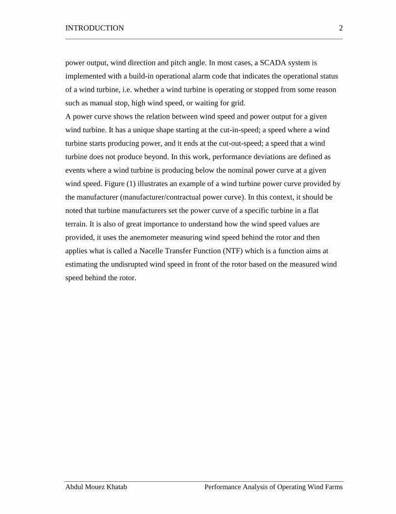
A power curve shows the relation between wind speed and power output for a given
wind turbine. It has a unique shape starting at the cut-in-speed; a speed where a wind
turbine starts producing power, and it ends at the cut-out-speed; a speed that a wind
turbine does not produce beyond. In this work, performance deviations are defined as
events where a wind turbine is producing below the nominal power curve at a given
wind speed. Figure (1) illustrates an example of a wind turbine power curve provided by
the manufacturer (manufacturer/contractual power curve). In this context, it should be
noted that turbine manufacturers set the power curve of a specific turbine in a flat
terrain. It is also of great importance to understand how the wind speed values are
provided, it uses the anemometer measuring wind speed behind the rotor and then
applies what is called a Nacelle Transfer Function (NTF) which is a function aims at
estimating the undisrupted wind speed in front of the rotor based on the measured wind
speed behind the rotor.
INTRODUCTION 3
Abdul Mouez Khatab Performance Analysis of Operating Wind Farms
Figure 1: Example of wind turbine power curve provided by the manufacturer. (“ERU Met Data - Wind Turbine
Power,” 2017)
Standard deviation is a measure of the dispersion of a set of data from its mean. It is
calculated as the square root of variance by determining the variation between each data
point relative to the mean. If the data points are further from the mean, there is higher
deviation within the data set (“Standard Deviation,” 2017).
1.3. Objective and Research Questions
While most of the research within this field is mainly about condition monitoring and
costly power test performance in compliance with the International Electrotechnical
Commission (IEC) standards, few reports have addressed performance analysis via use
of SCADA (Supervisory Control And Data Acquisition) data. This thesis has attempted
to deliver a practical, quick and convenient way to assess the performance of an
operating wind farm via use of SCADA and modeled wind data. The method works
either as independent assessment tool or as a complementary tool for condition
monitoring system. The thesis will investigate the following questions:
• How much is the potential energy production?

INTRODUCTION 4
Abdul Mouez Khatab Performance Analysis of Operating Wind Farms
• How big is the production loss?
• What are the main reasons behind the observed losses?
• What measures can be taken in order to minimize the losses?
1.4. Justification of the Research
It is of great importance for the industrial community represented mainly by wind farm
operators and project managers to understand why wind turbines underperform. This
enables operators to either optimize the wind farm or further investigate a specific aspect
where a turbine/farm is underperforming. Accordingly, this will result in a number of
optimization measures, that in turn are expected to increase the profitability of the wind
farm.
1.5. Methodology
The assessment of a wind farm will be executed by calculating the Potential
Energy Production, which is the ideal annual energy output with no loss at all and 100%
availability. This is done by taking the operational power curve of the respective year as
a reference and then applying it to the wind resources determined from Weibull
distribution. The operational power curve is a representative power curve of a specific
turbine. It takes into account the valid historical events where the turbine is in normal
operation. This power curve is exhibits higher representativeness of the turbine
performance than the contractual power curve provided by manufacturer. Losses will be
calculated and categorized to evaluate the main reasons behind the underperformance.
Determination of the necessary measures to mitigate losses will be done. A case study is
investigated in order to assess the methodology. The proposed methodology is
thoroughly explained in chapter 3.
1.6. Outline
Chapter 2 discusses the literature related to the topic. Mainly within the fields of
data mining, performance analysis and optimization of wind turbines performance. Next,
in chapter 3, the followed methodology is thoroughly explained after presenting a flow

INTRODUCTION 5
Abdul Mouez Khatab Performance Analysis of Operating Wind Farms
chart showing the frame work. In chapter 4, a case study is presented and further
analyzed in order to evaluate the proposed methodology. The same chapter presents the
results and discusses the outcomes of the investigated case study. Finally, chapter 5
draws a number of conclusion, enlists the limitations, and make suggestions for future
work.
LITERATURE REVIEW 6
Abdul Mouez Khatab Performance Analysis of Operating Wind Farms
2. LITERATURE REVIEW
2.1. Introduction
In this chapter, methodologies, findings, and features of previous studies investigating
the topics related to this work are discussed and analyzed. It starts by stating the work
done with the objective of understanding and analyzing the performance of wind
turbines in section 2.2. It then previews works that implemented SCADA data for
performance evaluation and loss assessment in section 2.3. Main reasons behind
underperformance and losses proposed by previous papers are stated and discussed in
section 2.4. In the next section 2.5, the measures utilized for performance enhancement
are presented and discussed. Finally, conclusions are drawn by the end of this chapter,
section 2.6, to spot the main features of the literature review.
2.2. Performance Analysis
The consistent aim of maximizing the revenues from a wind farm poses a huge need for
understanding the way the machines perform. In this area, three main topics have
attracted researchers the most: power performance, directional behavior, and pitch
mechanism.
2.2.1. Power Performance Test
As power is the fundamental product of wind turbines, it makes sense for researchers to
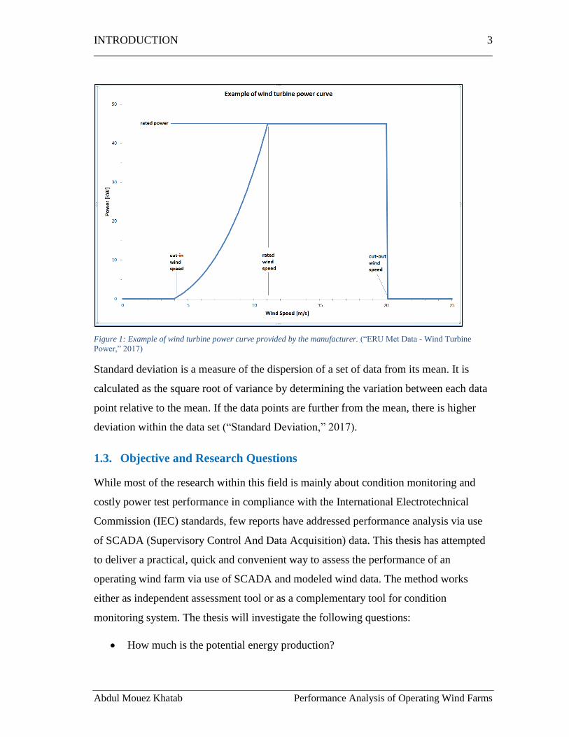
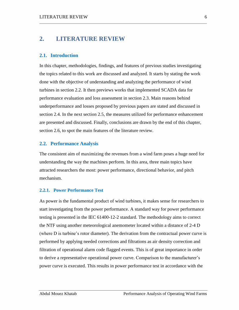
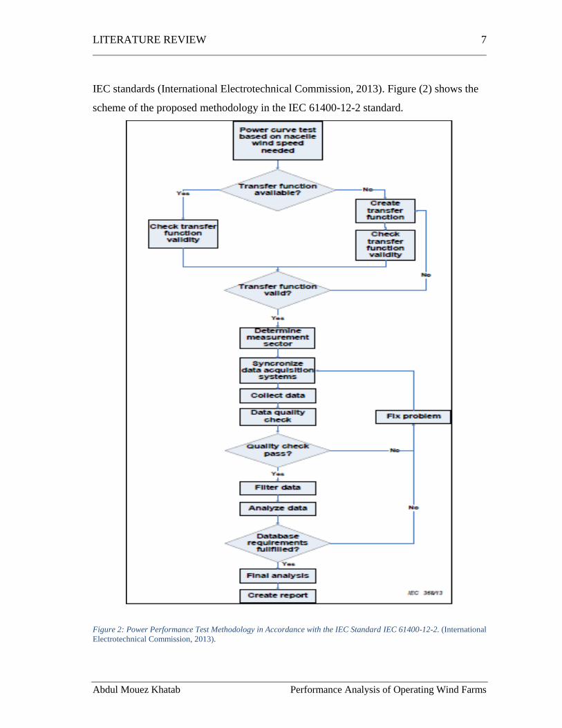
start investigating from the power performance. A standard way for power performance
testing is presented in the IEC 61400-12-2 standard. The methodology aims to correct
the NTF using another meteorological anemometer located within a distance of 2-4 D
(where D is turbine’s rotor diameter). The derivation from the contractual power curve is
performed by applying needed corrections and filtrations as air density correction and
filtration of operational alarm code flagged events. This is of great importance in order
to derive a representative operational power curve. Comparison to the manufacturer’s
power curve is executed. This results in power performance test in accordance with the
LITERATURE REVIEW 7
Abdul Mouez Khatab Performance Analysis of Operating Wind Farms
IEC standards (International Electrotechnical Commission, 2013). Figure (2) shows the
scheme of the proposed methodology in the IEC 61400-12-2 standard.
Figure 2: Power Performance Test Methodology in Accordance with the IEC Standard IEC 61400-12-2. (International
Electrotechnical Commission, 2013).
LITERATURE REVIEW 8
Abdul Mouez Khatab Performance Analysis of Operating Wind Farms
However, Kim et al. (2013) succeeded in conducting a power performance test of a wind
turbine located at a distance about 11 D to the met mast in compliance with the
procedure provided in the IEC 61400-12-2 standard. The team concluded that the new
method is valid and it can reduce costs significantly in comparison to the one proposed
in the IEC 61400-12-2 standard since one met mast can be used for a higher number of
turbines even those located at longer distances. In both cases, the presence of an external
source for measuring the undisturbed wind flow in front of the rotor is a requirement,
although located at different distances from the targeted turbine for power testing, 2-4 D
in the IEC 61400-12-2 standards and > 4D in Kim et al. (2013). This entails high costs
for wind farm operators.
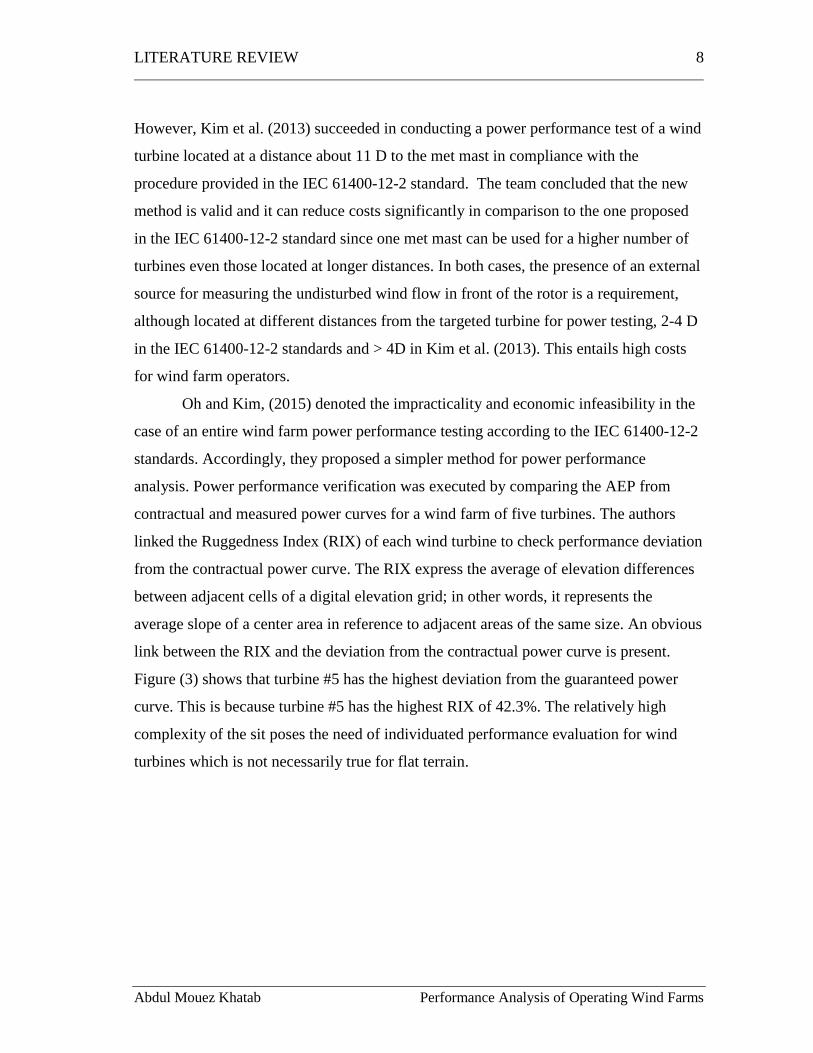
Oh and Kim, (2015) denoted the impracticality and economic infeasibility in the
case of an entire wind farm power performance testing according to the IEC 61400-12-2
standards. Accordingly, they proposed a simpler method for power performance
analysis. Power performance verification was executed by comparing the AEP from
contractual and measured power curves for a wind farm of five turbines. The authors
linked the Ruggedness Index (RIX) of each wind turbine to check performance deviation
from the contractual power curve. The RIX express the average of elevation differences
between adjacent cells of a digital elevation grid; in other words, it represents the
average slope of a center area in reference to adjacent areas of the same size. An obvious
link between the RIX and the deviation from the contractual power curve is present.
Figure (3) shows that turbine #5 has the highest deviation from the guaranteed power
curve. This is because turbine #5 has the highest RIX of 42.3%. The relatively high
complexity of the sit poses the need of individuated performance evaluation for wind
turbines which is not necessarily true for flat terrain.
LITERATURE REVIEW 9
Abdul Mouez Khatab Performance Analysis of Operating Wind Farms
Figure 3: Deviation between measured and guaranteed power curves. (Oh and Kim, 2015).
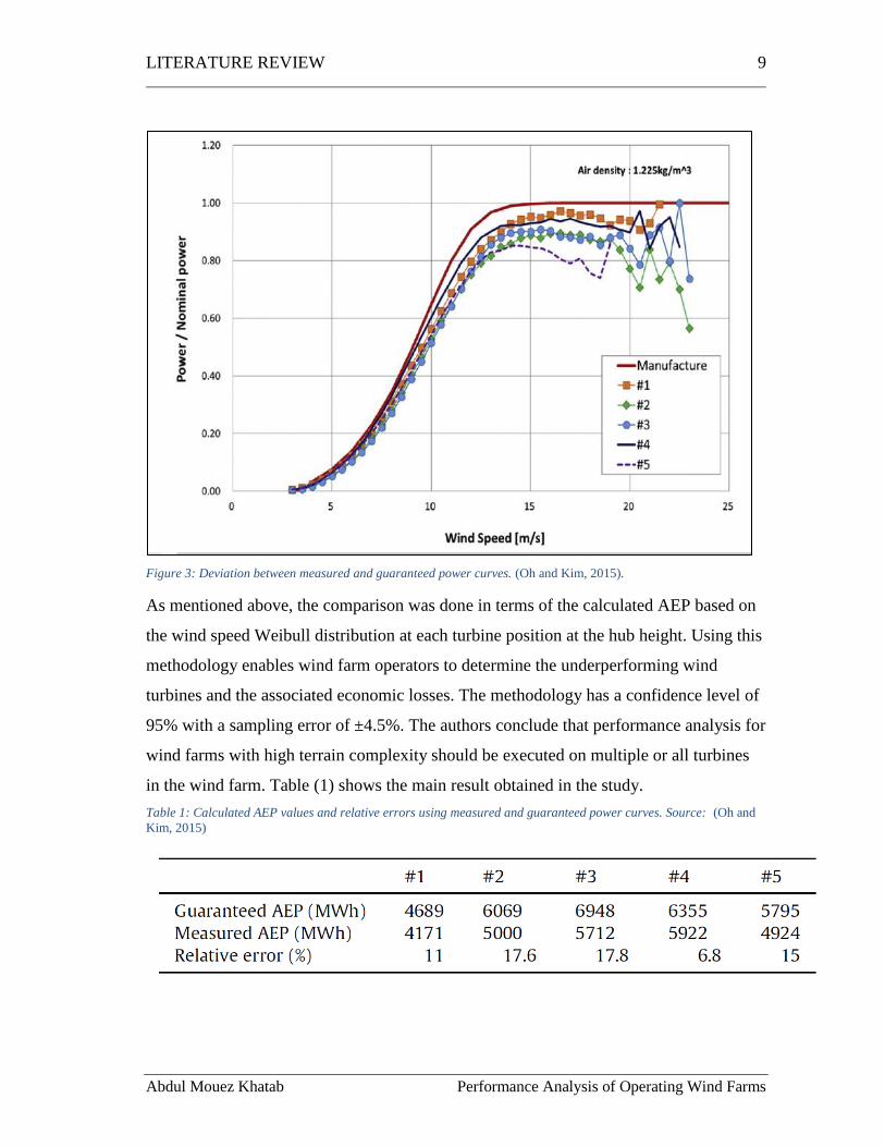
As mentioned above, the comparison was done in terms of the calculated AEP based on
the wind speed Weibull distribution at each turbine position at the hub height. Using this
methodology enables wind farm operators to determine the underperforming wind
turbines and the associated economic losses. The methodology has a confidence level of
95% with a sampling error of ±4.5%. The authors conclude that performance analysis for
wind farms with high terrain complexity should be executed on multiple or all turbines
in the wind farm. Table (1) shows the main result obtained in the study.
Table 1: Calculated AEP values and relative errors using measured and guaranteed power curves. Source: (Oh and
Kim, 2015)
LITERATURE REVIEW 10
Abdul Mouez Khatab Performance Analysis of Operating Wind Farms
Another approach based on the contractual power curve is found in the work of Nymfa
Noppe, (2014). The methodology entails calculating the operational power curve based
on the IEC 61400-12-2 standard and after that comparing it to the contractual power
curve. Three main steps are included in the calculation of the operational power curve:
• Filtering the data.
• Applying the needed corrections e.g. air density.
• Operational power curve calculation.
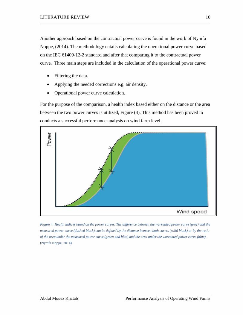
For the purpose of the comparison, a health index based either on the distance or the area
between the two power curves is utilized, Figure (4). This method has been proved to
conducts a successful performance analysis on wind farm level.
Figure 4: Health indices based on the power curves. The difference between the warranted power curve (grey) and the
measured power curve (dashed black) can be defined by the distance between both curves (solid black) or by the ratio
of the area under the measured power curve (green and blue) and the area under the warranted power curve (blue).
(Nymfa Noppe, 2014).
LITERATURE REVIEW 11
Abdul Mouez Khatab Performance Analysis of Operating Wind Farms
2.2.2. Directional Behavior
Plenty of research has been done to understand the overall performance of wind turbines,
though from different points of view. For instance, the analysis of the directional
behavior of individual wind turbines, cluster of wind turbines or collective behavior of a
wind farm yaw system, was investigated by the studies of Castellani et al, (2015a,
2015b) Turkyilmaz et al, (2016). In the study of Castellani et al. (2015b), the team
analyzed the performance of a cluster of wind turbines using SCADA data in addition to
data from nearby met mast. They emphasized that cluster analysis is a better practice
than considering the wind farm as one block or a number of individual units of turbines
since it results in higher accuracy and more accurate judgment of the performance.
Choosing one sector representing the dominant wind direction and then discretizing it to
finer sectors, they concluded that performance variations are caused by the response of
the cluster to the external conditions rather than the turbine themselves. Moreover, they
concluded that the most prevalent pattern of nacelle directions of the cluster is not the
optimal one. The same team conducted a separate analysis to relate wake effects to the
wind direction misalignment, hence, assessing the overall efficiency of the wind farm
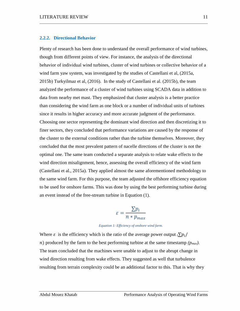
(Castellani et al., 2015a). They applied almost the same aforementioned methodology to
the same wind farm. For this purpose, the team adjusted the offshore efficiency equation
to be used for onshore farms. This was done by using the best performing turbine during
an event instead of the free-stream turbine in Equation (1).
𝜀 =∑𝑝𝑖
𝑛 ∗ 𝑝𝑚𝑎𝑥
Equation 1: Efficiency of onshore wind farm.
Where 𝜀 is the efficiency which is the ratio of the average power output (∑𝑝𝑖/
𝑛) produced by the farm to the best performing turbine at the same timestamp (pmax).
The team concluded that the machines were unable to adjust to the abrupt change in
wind direction resulting from wake effects. They suggested as well that turbulence
resulting from terrain complexity could be an additional factor to this. That is why they
LITERATURE REVIEW 12
Abdul Mouez Khatab Performance Analysis of Operating Wind Farms
recommended a future work assessing a more complex terrain using the same
methodology.
As a part of the extensive project “Assessment and optimization of the energy
production of operational wind farms”, Turkyilmaz et al. (2016) tackled the aspect of
directional behavior by installing a nacelle mounted lidar. One of the objectives was to
assess the misalignment in the yaw system by comparing SCADA data and data obtained
from the lidar.
Seemingly, nacelle misalignment to the real wind direction is a serious cause of
underperformance which contributes to financial loss. Correcting nacelle direction
requires an external source of wind direction, i.e. met mast or nacelle mounted lidar.
2.2.3. Pitch Mechanism
Pitch angle is another aspect that may cause performance deviation from the contractual
power curve. As a result, number of investigations have tackled this issue. Zhang (2012),
investigated the relationship between generator torque and pitch angle in order to reach
the optimal set of these two parameters by starting from tower acceleration and drive
train vibration. Godwin and Matthews (2013) stated that an electrical control system
fault leads to higher degradation of mechanical parts, underperformance events, and
higher costs of Operation and Maintenance (O&M). Therefore, they have investigated
performance of pitch mechanism and delivered a tool that classifies the status of pitch
system. The tool indicates normal condition, potential fault occurrence, and fault
detection aiming to avoid unscheduled O&M.
2.3. Utilization of SCADA System in Loss/Underperformance Assessment
2.3.1. Loss Assessment
Using SCADA data for assessing performance of wind turbines through loss calculation
is a highly under investigated topic. Only a handful of researchers has published studies
covering this issue. As part of the extensive project “Assessment and optimization of the
energy production of operational wind farms”, Lindvall et al. (2016) attempted to assess
LITERATURE REVIEW 13
Abdul Mouez Khatab Performance Analysis of Operating Wind Farms
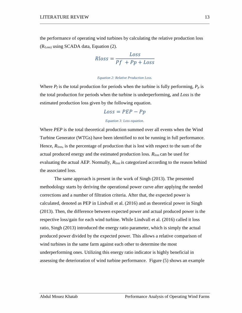
the performance of operating wind turbines by calculating the relative production loss
(RLoss) using SCADA data, Equation (2).
𝑅𝑙𝑜𝑠𝑠 =𝐿𝑜𝑠𝑠
𝑃𝑓 + 𝑃𝑝 + 𝐿𝑜𝑠𝑠
Equation 2: Relative Production Loss.
Where Pf is the total production for periods when the turbine is fully performing, Pp is
the total production for periods when the turbine is underperforming, and Loss is the
estimated production loss given by the following equation.
𝐿𝑜𝑠𝑠 = 𝑃𝐸𝑃 − 𝑃𝑝
Equation 3: Loss equation.
Where PEP is the total theoretical production summed over all events when the Wind
Turbine Generator (WTGs) have been identified to not be running in full performance.
Hence, Rloss, is the percentage of production that is lost with respect to the sum of the
actual produced energy and the estimated production loss. Rloss can be used for
evaluating the actual AEP. Normally, Rloss is categorized according to the reason behind
the associated loss.
The same approach is present in the work of Singh (2013). The presented
methodology starts by deriving the operational power curve after applying the needed
corrections and a number of filtration criteria. After that, the expected power is
calculated, denoted as PEP in Lindvall et al. (2016) and as theoretical power in Singh
(2013). Then, the difference between expected power and actual produced power is the
respective loss/gain for each wind turbine. While Lindvall et al. (2016) called it loss
ratio, Singh (2013) introduced the energy ratio parameter, which is simply the actual
produced power divided by the expected power. This allows a relative comparison of
wind turbines in the same farm against each other to determine the most
underperforming ones. Utilizing this energy ratio indicator is highly beneficial in
assessing the deterioration of wind turbine performance. Figure (5) shows an example
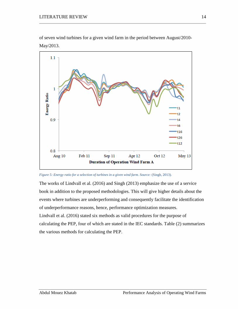
LITERATURE REVIEW 14
Abdul Mouez Khatab Performance Analysis of Operating Wind Farms
of seven wind turbines for a given wind farm in the period between August/2010-
May/2013.
Figure 5: Energy ratio for a selection of turbines in a given wind farm. Source: (Singh, 2013).
The works of Lindvall et al. (2016) and Singh (2013) emphasize the use of a service
book in addition to the proposed methodologies. This will give higher details about the
events where turbines are underperforming and consequently facilitate the identification
of underperformance reasons, hence, performance optimization measures.
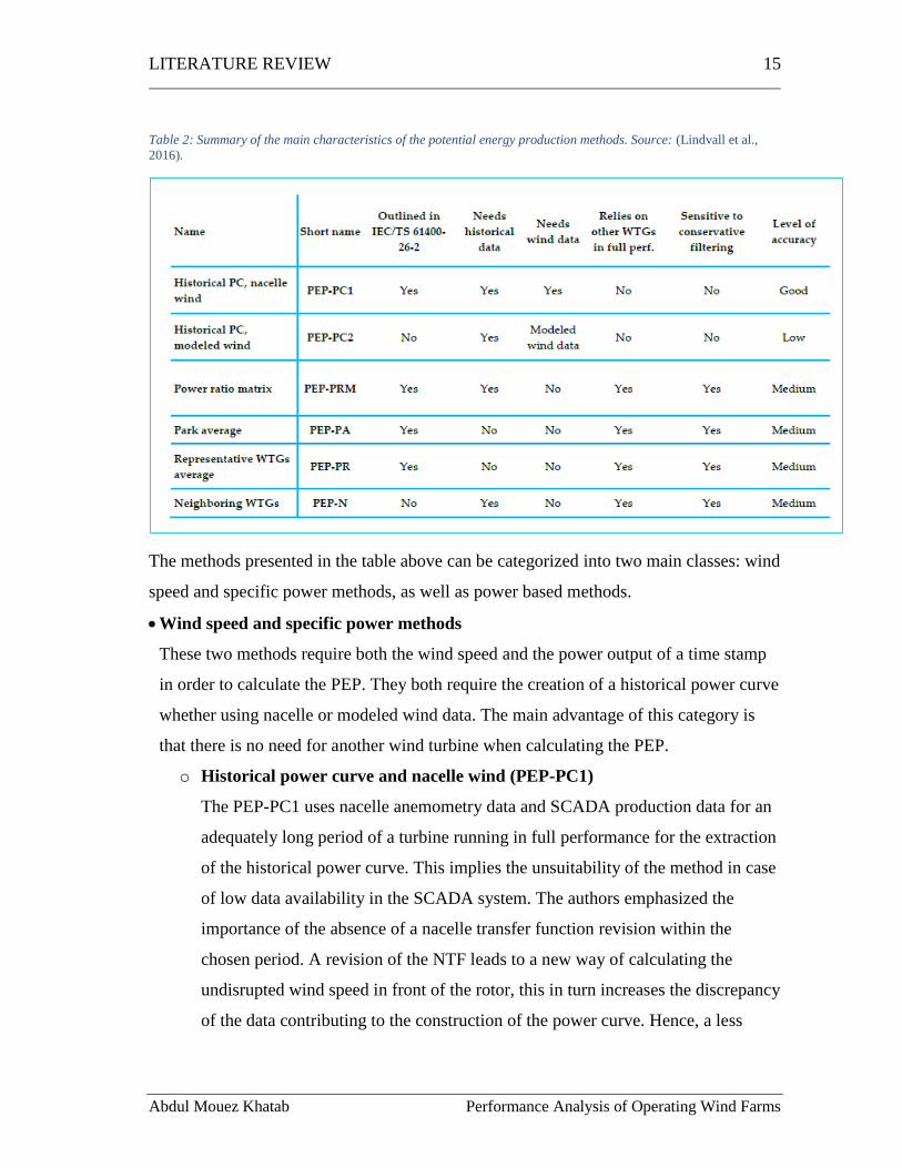
Lindvall et al. (2016) stated six methods as valid procedures for the purpose of
calculating the PEP, four of which are stated in the IEC standards. Table (2) summarizes
the various methods for calculating the PEP.
LITERATURE REVIEW 15
Abdul Mouez Khatab Performance Analysis of Operating Wind Farms
Table 2: Summary of the main characteristics of the potential energy production methods. Source: (Lindvall et al.,
2016).
The methods presented in the table above can be categorized into two main classes: wind
speed and specific power methods, as well as power based methods.
• Wind speed and specific power methods
These two methods require both the wind speed and the power output of a time stamp
in order to calculate the PEP. They both require the creation of a historical power curve
whether using nacelle or modeled wind data. The main advantage of this category is
that there is no need for another wind turbine when calculating the PEP.
o Historical power curve and nacelle wind (PEP-PC1)
The PEP-PC1 uses nacelle anemometry data and SCADA production data for an
adequately long period of a turbine running in full performance for the extraction
of the historical power curve. This implies the unsuitability of the method in case
of low data availability in the SCADA system. The authors emphasized the
importance of the absence of a nacelle transfer function revision within the
chosen period. A revision of the NTF leads to a new way of calculating the
undisrupted wind speed in front of the rotor, this in turn increases the discrepancy
of the data contributing to the construction of the power curve. Hence, a less
LITERATURE REVIEW 16
Abdul Mouez Khatab Performance Analysis of Operating Wind Farms
representative power curve results and this invalidates the proposed method for
the calculations of the PEP. The authors proposed a method as well for assuring
the absence of such a period by comparing two neighboring turbines for wake
free occasions of full and partial performance. After the creation of the historical
power curve, PEP can be calculated expecting all underperforming events to have
their power output in accordance with the historical power curve. The authors
considered this method as the most accurate among the proposed methods since it
relies on both measured wind speed and power output, which in turn exhibits less
uncertainty.
o Historical power curve and modeled wind (PEP-PC2)
The historical power curve is derived using the filtered wind data and the
concurrent modeled Weather Research and Forecast (WRF) wind speed in order
to extract the historical power curve. Only events where the turbine is in full
performance are used. It should be taken into consideration that sector-wise
historical power curves shall be constructed to account for wake effects. For the
PEP calculation, the PEP-PC2 method applies WRF modeled data (wind speed
and wind direction) to the derived historical power curve. This method has a
disadvantage of low accuracy since it utilizes modeled wind speed instead of
measured.
• Power based methods
This group is dependent on data from another wind turbine. The main idea is that for
a given time stamp, there will be at least one turbine running in full performance.
This, however, entails that these methods are invalid in case of a park-wide
environment where the entire park is simultaneously underperforming due to an
external cause such as in harsh icing conditions.
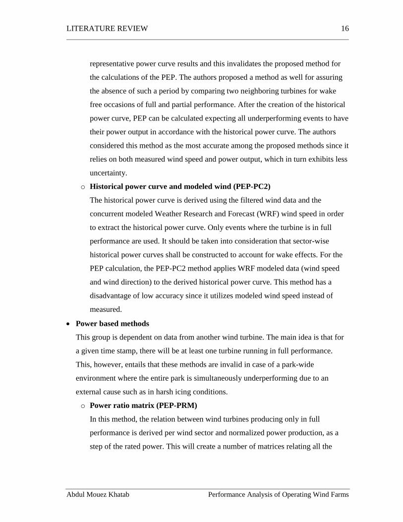
o Power ratio matrix (PEP-PRM)
In this method, the relation between wind turbines producing only in full
performance is derived per wind sector and normalized power production, as a
step of the rated power. This will create a number of matrices relating all the
LITERATURE REVIEW 17
Abdul Mouez Khatab Performance Analysis of Operating Wind Farms
turbines together for a specific wind direction at a specific power range. Figure
(6) shows the power ratio matrix for a given wind farm at wind direction
[195°,225°[ and normalized power range [0.72,0.76[.
Figure 6: Example of power ratio matrix for a given wind farm with 11 turbines. Source: (Lindvall et al., 2016).
Following this method, the PEP will be calculated by
o Identifying turbines in full performance.
o Based on wind direction and normalized power, choosing the respective
power ratio matrix.
o Calculate the average product of the inter-turbine relationship. For
example, if turbine #1 is underperforming and turbines #2 and #3 found to
be in full performance, the PEP of turbine #1 is then the average of the
ratios T1/T2 and T1/T3 derived from Figure (6) multiplied bu the
productions of T2 and T3 respectively
𝑃𝐸𝑃 𝑇1 =
𝑇1𝑇2 𝑝𝑟𝑜𝑑 𝑇2 +
𝑇1𝑇3 𝑝𝑟𝑜𝑑 𝑇3
2
LITERATURE REVIEW 18
Abdul Mouez Khatab Performance Analysis of Operating Wind Farms
o Park Average (PEP-PA)
According to this method, the PEP of an underperforming wind turbine is the
average of the fully performing wind turbines in the entire park for a given
occasion. For calculating the PEP, an average production factor is calculated in
compliance with the IEC 61400-26-2 as (actual power/rated power) for turbines
in full performance. The authors stated that this method is not applicable for wind
farms with highly unsymmetrical elevation.
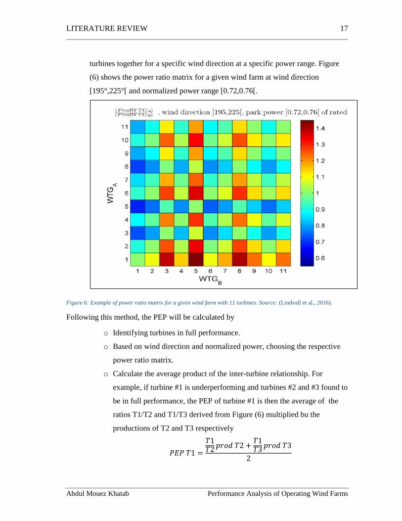
o Average of subset of representative WTGs (PEP-RA)
This method is very similar to the park average. The only difference is that the
factor is calculated for a subset of representative WTGs instead of the entire park.
The representativeness is mainly judged on wind farm layout, wake effects and
wind level. Table (3) shows an example of a given wind farm.
Table 3: Group of representative WTGs for a given wind farm of 11 turbines. Source: (Lindvall et al., 2016).
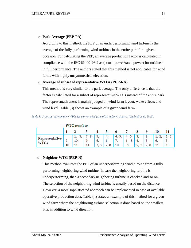
o Neighbor WTG (PEP-N)
This method evaluates the PEP of an underperforming wind turbine from a fully
performing neighboring wind turbine. In case the neighboring turbine is
underperforming, then a secondary neighboring turbine is checked and so on.
The selection of the neighboring wind turbine is usually based on the distance.
However, a more sophisticated approach can be implemented in case of available
operative production data. Table (4) states an example of this method for a given
wind farm where the neighboring turbine selection is done based on the smallest
bias in addition to wind direction.
LITERATURE REVIEW 19
Abdul Mouez Khatab Performance Analysis of Operating Wind Farms
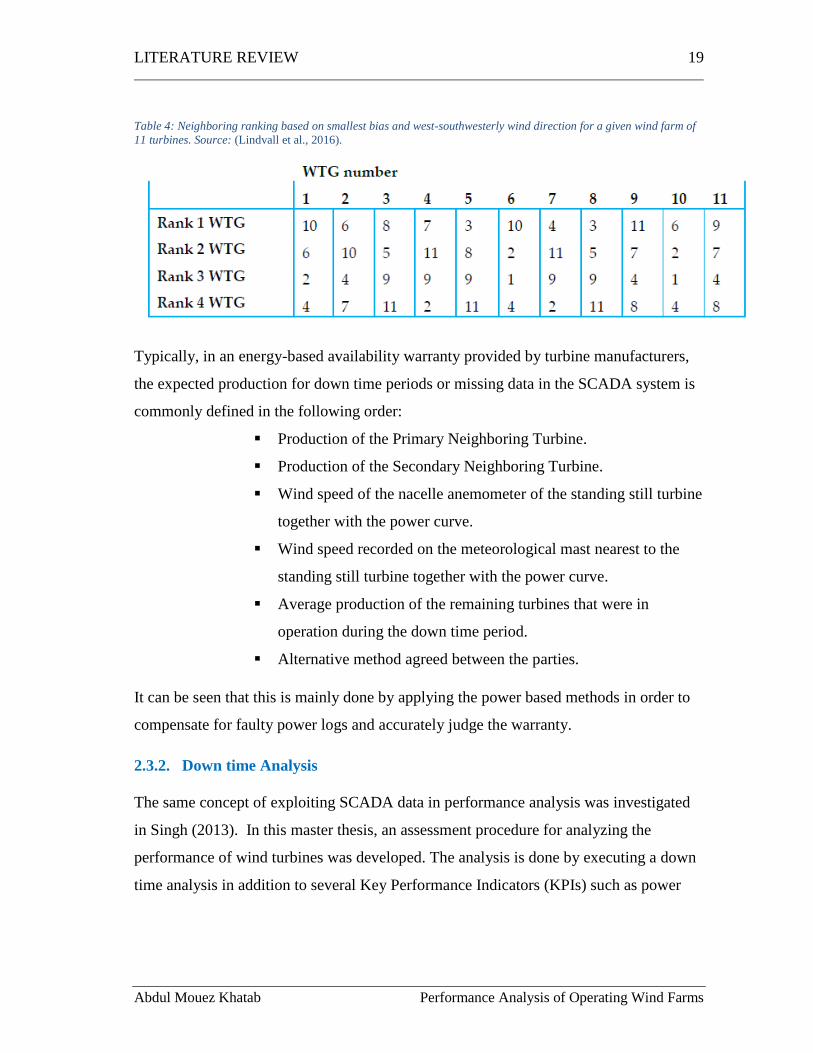
Table 4: Neighboring ranking based on smallest bias and west-southwesterly wind direction for a given wind farm of
11 turbines. Source: (Lindvall et al., 2016).
Typically, in an energy-based availability warranty provided by turbine manufacturers,
the expected production for down time periods or missing data in the SCADA system is
commonly defined in the following order:
▪ Production of the Primary Neighboring Turbine.
▪ Production of the Secondary Neighboring Turbine.
▪ Wind speed of the nacelle anemometer of the standing still turbine
together with the power curve.
▪ Wind speed recorded on the meteorological mast nearest to the
standing still turbine together with the power curve.
▪ Average production of the remaining turbines that were in
operation during the down time period.
▪ Alternative method agreed between the parties.
It can be seen that this is mainly done by applying the power based methods in order to
compensate for faulty power logs and accurately judge the warranty.
2.3.2. Down time Analysis
The same concept of exploiting SCADA data in performance analysis was investigated
in Singh (2013). In this master thesis, an assessment procedure for analyzing the
performance of wind turbines was developed. The analysis is done by executing a down
time analysis in addition to several Key Performance Indicators (KPIs) such as power
LITERATURE REVIEW 20
Abdul Mouez Khatab Performance Analysis of Operating Wind Farms
curve shape, energy ratio, pitch curve, yaw effects, rotor & generator speed, and torque
characteristics.
Three major keys are used to assess the down time based on the data provided in the
SCADA system:
✓ Number of down time events.
✓ Duration of events.
✓ Duration of time between events.
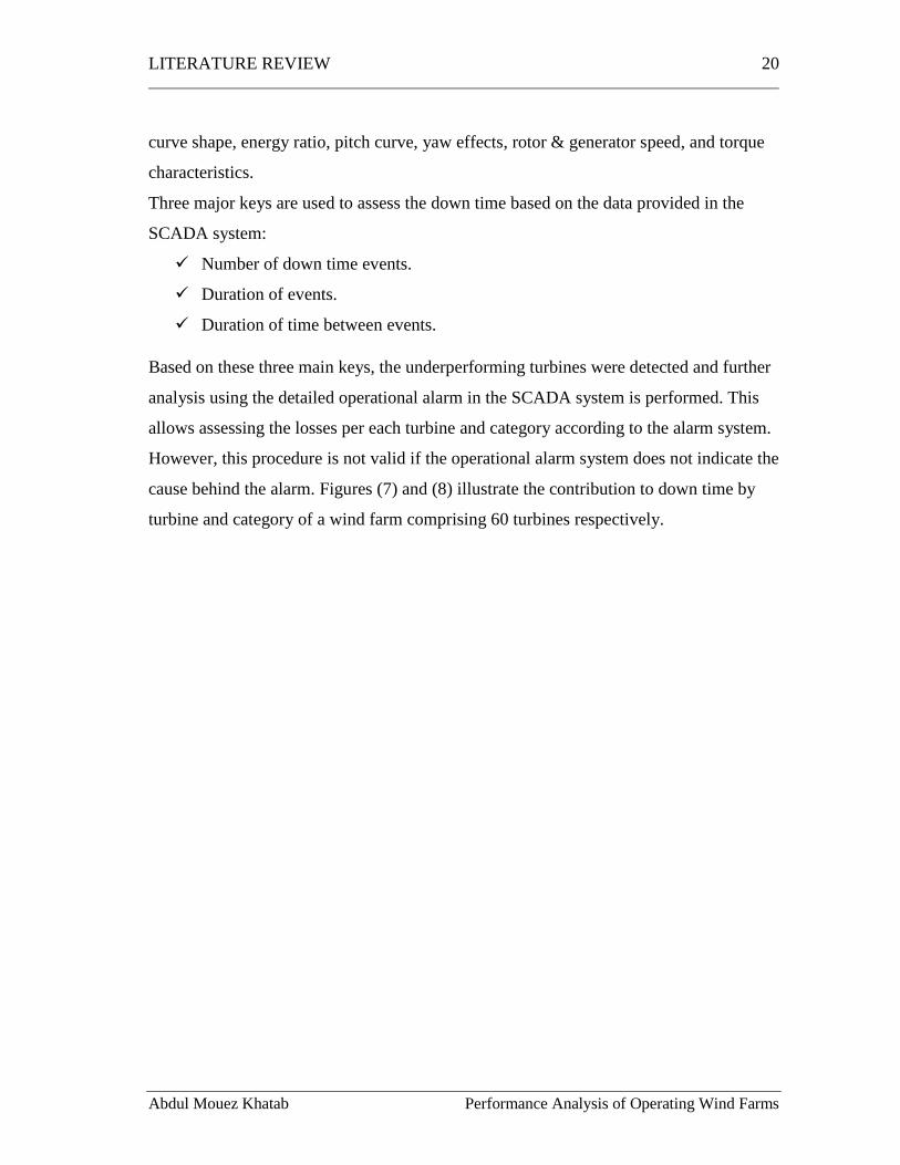
Based on these three main keys, the underperforming turbines were detected and further
analysis using the detailed operational alarm in the SCADA system is performed. This
allows assessing the losses per each turbine and category according to the alarm system.
However, this procedure is not valid if the operational alarm system does not indicate the
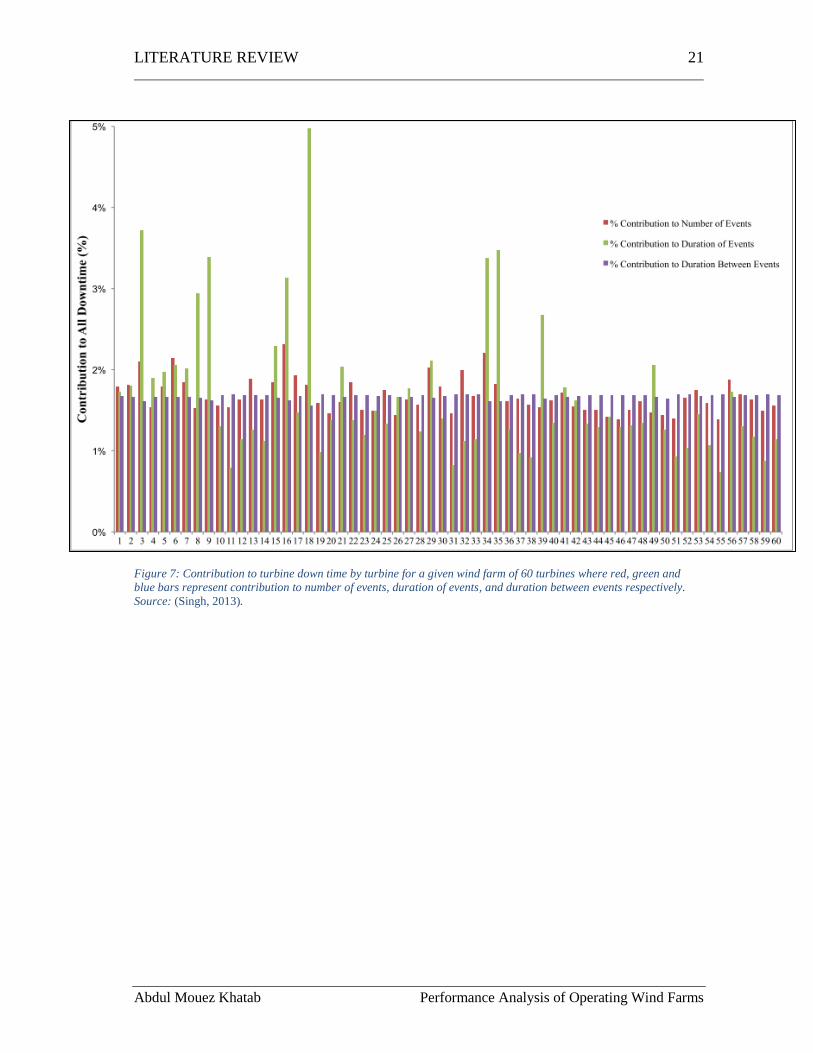
cause behind the alarm. Figures (7) and (8) illustrate the contribution to down time by
turbine and category of a wind farm comprising 60 turbines respectively.
LITERATURE REVIEW 21
Abdul Mouez Khatab Performance Analysis of Operating Wind Farms
Figure 7: Contribution to turbine down time by turbine for a given wind farm of 60 turbines where red, green and
blue bars represent contribution to number of events, duration of events, and duration between events respectively.
Source: (Singh, 2013).
LITERATURE REVIEW 22
Abdul Mouez Khatab Performance Analysis of Operating Wind Farms
Figure 8: Contribution to turbine down time per category for a given wind farm of 60 turbines. Source: (Singh, 2013).
These two analyses allow wind farm operators of detecting the turbines incurring higher
energy loss. It determines also which subsystem is responsible for higher down time
losses. Accordingly, the needed measures in order to optimize the performance can be
applied.
2.3.3. Icing Detection and Quantification
While the operational alarm covers a variety of reasons behind the flagged events, as
discussed in section (2.3.2), the detection and calculation of down time periods and
losses is somehow uncomplicated. On the contrary, detection and quantification of icing
losses are of high complexity due to a high number of factors contributing to the icing
phenomena. Among the strongest studies attempting to detect and quantify icing losses
is the study of Davis et al. (2015). This study investigates three different threshold
methodologies to account for icing losses based on the operational power curve. All
three methodologies determine an icing threshold which indicates the formation of
LITERATURE REVIEW 23
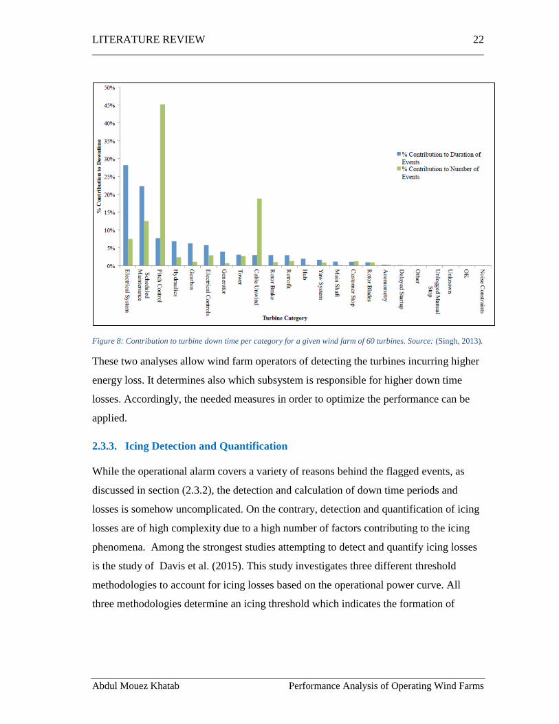
Abdul Mouez Khatab Performance Analysis of Operating Wind Farms
instrumental icing. Table (5) summarizes the methodologies, threshold calculation and
the results presented by Davis et al. (2015).
Table 5: The methodologies suggested by Davis et al. (2015) for icing loss calculation. Source: (Davis et al., 2015).
Methodology Description Advantages Disadvantages
Flat Percentage The threshold is a
fixed percentage of
the manufacturer’s
power curve;
common values
range between
7.5% to 20%.
No need for
historical data or
data cleaning.
Does not capture
the impact of local
effects as wakes
and topography.
Not representative
for individual
turbines. May lead
to either under- or
overestimation
Standard
Deviation
The threshold is
defined based on
the variance to the
observed power
curve by
calculating the
standard deviation
per each bin.
Does not rely on
manufacturer’s
power curve.
Does not perform
well on non-usual
distributions.
Needs a smoothing
function.
Quantile The threshold is a
specific quantile
per each bin of the
observed power
curve.
Does not need
smoothing
functions.
Does not rely on
manufacturer’s
power curve.
Needs LOSS
smoother.
LITERATURE REVIEW 24
Abdul Mouez Khatab Performance Analysis of Operating Wind Farms
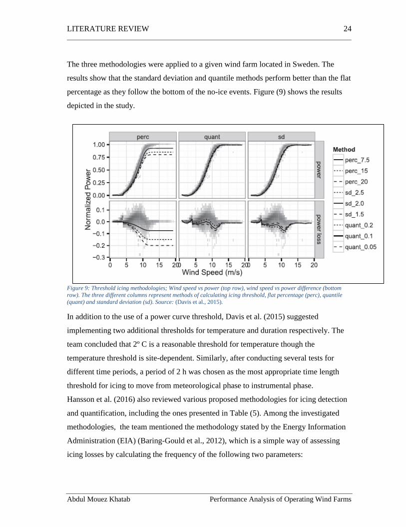
The three methodologies were applied to a given wind farm located in Sweden. The
results show that the standard deviation and quantile methods perform better than the flat
percentage as they follow the bottom of the no-ice events. Figure (9) shows the results
depicted in the study.
Figure 9: Threshold icing methodologies; Wind speed vs power (top row), wind speed vs power difference (bottom
row). The three different columns represent methods of calculating icing threshold, flat percentage (perc), quantile
(quant) and standard deviation (sd). Source: (Davis et al., 2015).
In addition to the use of a power curve threshold, Davis et al. (2015) suggested
implementing two additional thresholds for temperature and duration respectively. The
team concluded that 2º C is a reasonable threshold for temperature though the
temperature threshold is site-dependent. Similarly, after conducting several tests for
different time periods, a period of 2 h was chosen as the most appropriate time length
threshold for icing to move from meteorological phase to instrumental phase.
Hansson et al. (2016) also reviewed various proposed methodologies for icing detection
and quantification, including the ones presented in Table (5). Among the investigated
methodologies, the team mentioned the methodology stated by the Energy Information
Administration (EIA) (Baring-Gould et al., 2012), which is a simple way of assessing
icing losses by calculating the frequency of the following two parameters:
LITERATURE REVIEW 25
Abdul Mouez Khatab Performance Analysis of Operating Wind Farms
1. Meteorological icing: periods where the meteorological conditions are
favorable for icing formation.
2. Instrumental icing: periods where ice is accumulated on a structure or an
instrument.
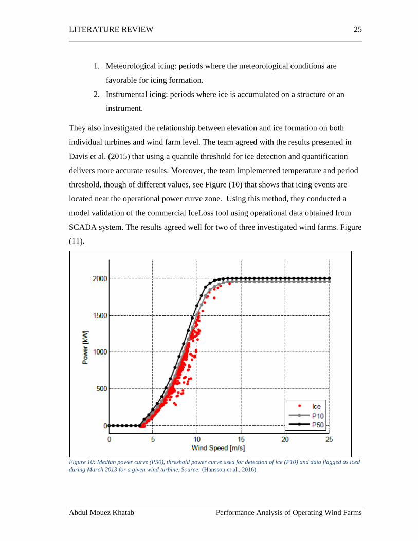
They also investigated the relationship between elevation and ice formation on both
individual turbines and wind farm level. The team agreed with the results presented in
Davis et al. (2015) that using a quantile threshold for ice detection and quantification
delivers more accurate results. Moreover, the team implemented temperature and period
threshold, though of different values, see Figure (10) that shows that icing events are
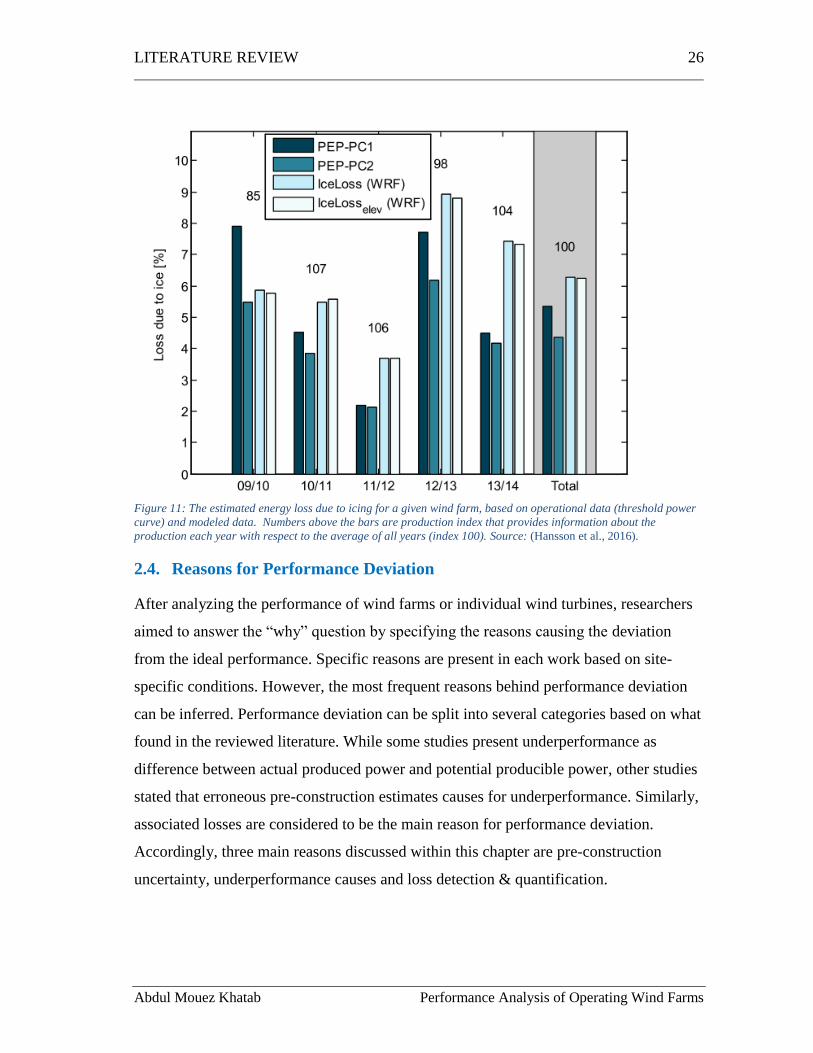
located near the operational power curve zone. Using this method, they conducted a
model validation of the commercial IceLoss tool using operational data obtained from
SCADA system. The results agreed well for two of three investigated wind farms. Figure
(11).
Figure 10: Median power curve (P50), threshold power curve used for detection of ice (P10) and data flagged as iced
during March 2013 for a given wind turbine. Source: (Hansson et al., 2016).
LITERATURE REVIEW 26
Abdul Mouez Khatab Performance Analysis of Operating Wind Farms
Figure 11: The estimated energy loss due to icing for a given wind farm, based on operational data (threshold power
curve) and modeled data. Numbers above the bars are production index that provides information about the
production each year with respect to the average of all years (index 100). Source: (Hansson et al., 2016).
2.4. Reasons for Performance Deviation
After analyzing the performance of wind farms or individual wind turbines, researchers
aimed to answer the “why” question by specifying the reasons causing the deviation
from the ideal performance. Specific reasons are present in each work based on site-
specific conditions. However, the most frequent reasons behind performance deviation
can be inferred. Performance deviation can be split into several categories based on what
found in the reviewed literature. While some studies present underperformance as
difference between actual produced power and potential producible power, other studies
stated that erroneous pre-construction estimates causes for underperformance. Similarly,
associated losses are considered to be the main reason for performance deviation.
Accordingly, three main reasons discussed within this chapter are pre-construction
uncertainty, underperformance causes and loss detection & quantification.
LITERATURE REVIEW 27
Abdul Mouez Khatab Performance Analysis of Operating Wind Farms
2.4.1. Pre-construction uncertainties
This category includes the reasons responsible for underperformance prior to the
construction of a wind farm. In the literature, this category can be referred to as “reasons
for uncertainty” as well “Underperformance causes”. It can be found in the studies of
Liléo et al. (2013), Turkyilmaz et al. (2016), and Tücer (2016) that the main reasons
standing behind the evaluated pre-construction uncertainties are as follows:
• Data Quality
This includes the data used in the Wind Resource Assessment (WRA). Namely, wind
measurements, elevation grid, and roughness data. The quality of the data is an essential
factor for an accurate judgment of the expected energy output (Tücer, 2016). Turkyilmaz
et al. (2016) stated that this category is referred to as “wind conditions” among
researchers. Power Curve Working Group (PCWG) agreed on a list of wind conditions
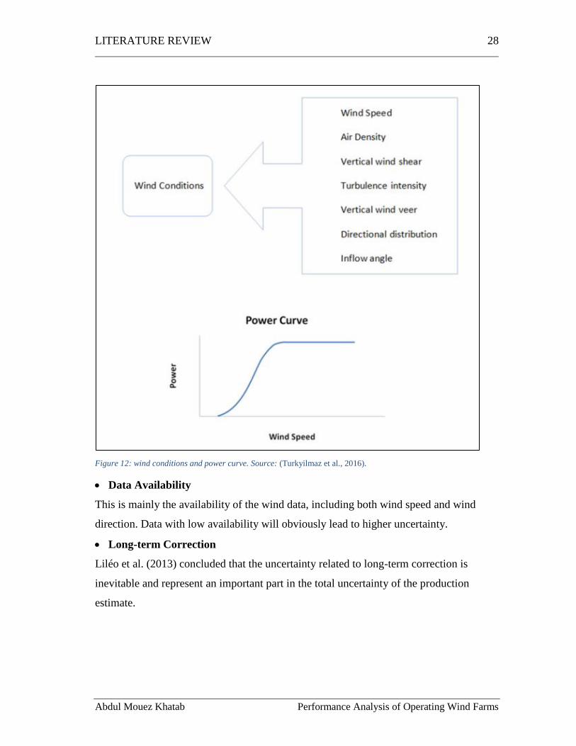
also referred as power curve parameters which can represent the main data in this
category, Figure (12).
LITERATURE REVIEW 28
Abdul Mouez Khatab Performance Analysis of Operating Wind Farms
Figure 12: wind conditions and power curve. Source: (Turkyilmaz et al., 2016).
• Data Availability
This is mainly the availability of the wind data, including both wind speed and wind
direction. Data with low availability will obviously lead to higher uncertainty.
• Long-term Correction
Liléo et al. (2013) concluded that the uncertainty related to long-term correction is
inevitable and represent an important part in the total uncertainty of the production
estimate.
LITERATURE REVIEW 29
Abdul Mouez Khatab Performance Analysis of Operating Wind Farms
• Used models
This includes used flow models in order to estimate the AEP. Tücer (2016) investigated
the uncertainties related to the choice of the software tool (WAsP or WindSim) as well
as the choice of various sub-models like the wake model.
2.4.2. Underperformance causes
Several researchers attempted to explain the reasons of underperforming wind turbines.
This category includes aspects which cause the turbine to underperform when it
expected to be in full performance. Most frequent reasons for the underperformance of
wind turbines amongst others are control parameters and NTF calibration.
• Control parameters
Several studies have pointed out the control parameters of the wind turbines as
underperformance causes. Plenty of studies have investigated the yaw system’s
functionality. The misalignment between the nacelle and the real wind direction may
subject the blades to higher turbulence. It also leads to energy losses as well as faster
degradation. Further details can be found in Castellani et al. (2015a) & (2015b) and
Turkyilmaz et al (2016).
Another control system that is perceived as cause of underperformance is pitch
mechanism. The pitch system adjusts the angle of the blades in order to extract the
optimal amount of energy from the wind. More details can be found in the work of Bi et
al. (2016).
• NTF calibration
A reasonable number of researchers have stated that the NFT has an impact on the
discrepancy when plotting wind speed vs. power output because the NFT cannot
precisely define the wind speed for the undisrupted stream in front of the rotor. Lindvall
et al. (2016) emphasized the importance of knowing the exact date of NTF revisions and
its impact when calculating a representative operational power curve.
LITERATURE REVIEW 30
Abdul Mouez Khatab Performance Analysis of Operating Wind Farms
• Other underperformance causes
Turkyilmaz et al. (2016) added curtailment and de-rated operation due to noise or
shadow restrictions to this category as they are related to the control system.
2.4.3. Production loss detection and quantification
• Component Failure
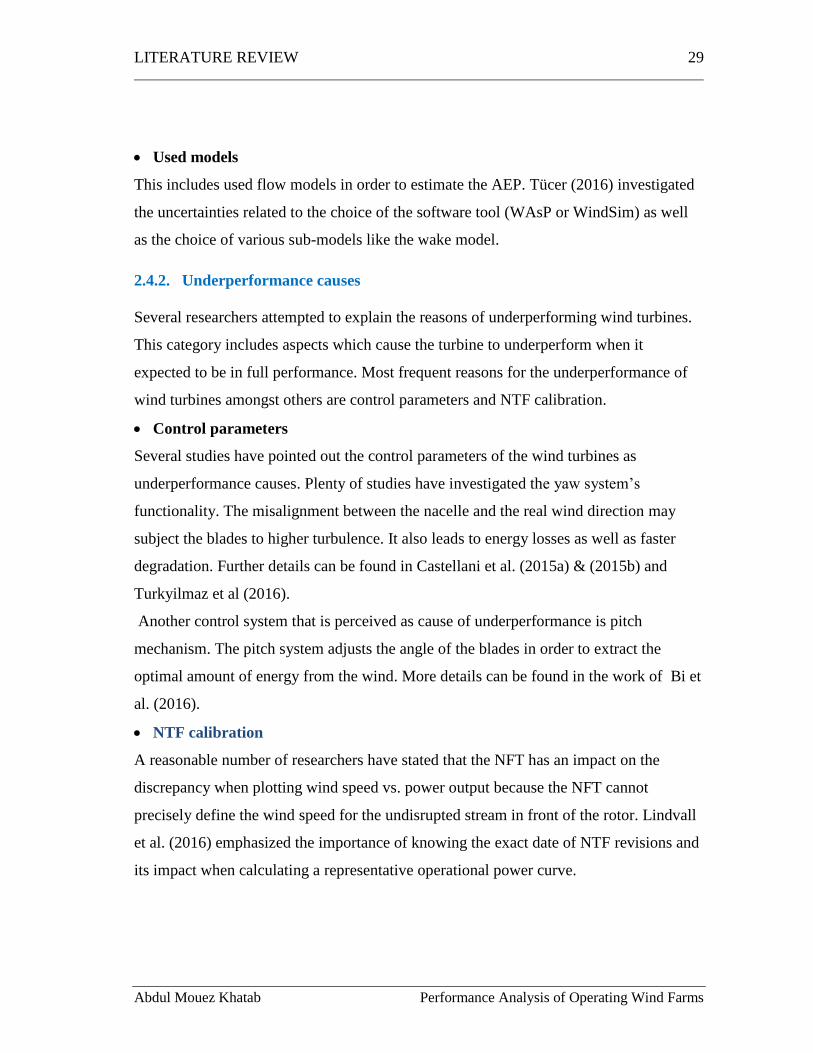
Component failure is the most contributing category to down time of wind farms. Thus,
it represents a reasonable share in financial losses. Several reports have been conducted
in order to understand which components contribute the most for down time and what
actions lead to better practice regarding maintenance and inspection. The reports of
Nivedh (2014) and Sheng (2013) conducted a statistical analysis on a large amount of
data in Europe and the US. The results are very similar in terms of down time per
component failure. Figure (13) shows the results of Sheng (2013)’s work.
Figure 13: Failure/Turbine/year and down time for two large surveys of onshore European wind turbines over 13
years. Source: (Sheng, 2013).
• Icing
Icing is a hot topic concerning wind farm operators in cold climate. The accumulation of
icing on the blades distorts the airfoil’s optimal shape and results in power output
LITERATURE REVIEW 31
Abdul Mouez Khatab Performance Analysis of Operating Wind Farms
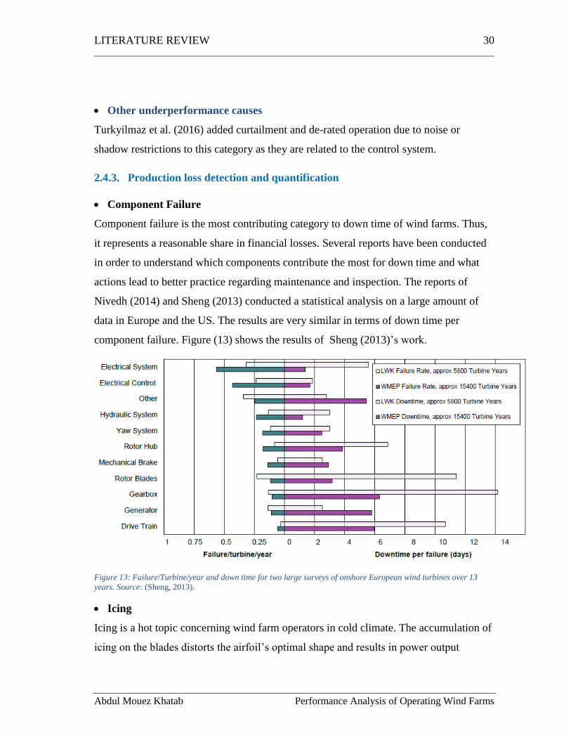
reduction. According to Hansson et al. (2016), icing can contribute to more than 10%
losses in sites subject to cold climate conditions. Sheng (2013) has even stated that icing
can lead to component failure, particularly the electric control units. Figure (14) shows
icing contribution to component failure.
Figure 14: Contributors to component failure. Source: (Sheng, 2013).
2.5. Optimization Measures
After analyzing the performance and detecting the proposed reasons behind the
underperformance. It is time to check what measures/actions can be taken in order to
enhance the performance of wind farms. As observed in the studied literature,
optimization measures can be split into two main tracks which are hardware installation
and parametric adjustment.
2.5.1. Hardware Installation
An obvious trend among both researchers and wind farm operators is to install a
condition monitoring system. Based on processing online historical data, a condition
LITERATURE REVIEW 32
Abdul Mouez Khatab Performance Analysis of Operating Wind Farms
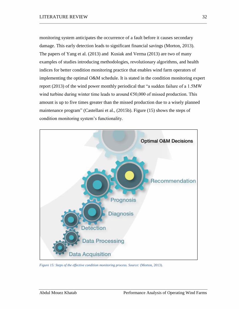
monitoring system anticipates the occurrence of a fault before it causes secondary
damage. This early detection leads to significant financial savings (Morton, 2013).
The papers of Yang et al. (2013) and Kusiak and Verma (2013) are two of many
examples of studies introducing methodologies, revolutionary algorithms, and health
indices for better condition monitoring practice that enables wind farm operators of
implementing the optimal O&M schedule. It is stated in the condition monitoring expert
report (2013) of the wind power monthly periodical that “a sudden failure of a 1.5MW
wind turbine during winter time leads to around €50,000 of missed production. This
amount is up to five times greater than the missed production due to a wisely planned
maintenance program” (Castellani et al., (2015b). Figure (15) shows the steps of
condition monitoring system’s functionality.
Figure 15: Steps of the effective condition monitoring process. Source: (Morton, 2013).
LITERATURE REVIEW 33
Abdul Mouez Khatab Performance Analysis of Operating Wind Farms
Likewise, installation of a nacelle-mounted lidar is becoming more common
nowadays. Its main aim is to adjust the misalignment between the nacelle and real
wind direction. Turkyilmaz et al. (2016) installed a lidar on the top of several wind
turbines in different sites. They were able to optimize the power output by correcting
the yaw system misalignment. For a given turbine in one of the wind farms a yaw
error of -2.4º was detected with a confidence of 95%. The yaw misalignment
correction would result in 0.3% gain in the AEP, see Table (6). Moreover, the
installation of the lidar allowed recalibrating the NTF.
LITERATURE REVIEW 34
Abdul Mouez Khatab Performance Analysis of Operating Wind Farms
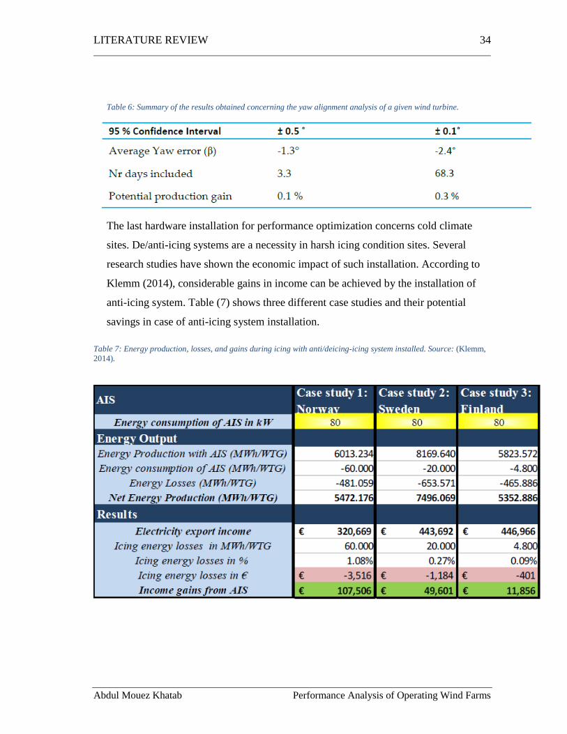
Table 6: Summary of the results obtained concerning the yaw alignment analysis of a given wind turbine.
The last hardware installation for performance optimization concerns cold climate
sites. De/anti-icing systems are a necessity in harsh icing condition sites. Several
research studies have shown the economic impact of such installation. According to
Klemm (2014), considerable gains in income can be achieved by the installation of
anti-icing system. Table (7) shows three different case studies and their potential
savings in case of anti-icing system installation.
Table 7: Energy production, losses, and gains during icing with anti/deicing-icing system installed. Source: (Klemm,
2014).
LITERATURE REVIEW 35
Abdul Mouez Khatab Performance Analysis of Operating Wind Farms
2.5.2. Parametric Adjustment
A number of researchers concerned themselves with reducing the cost of energy
rather than maximizing energy output. This indeed will result in a reduction in
investment costs and eventually lead to optimal economic parameters like Net Present
Value (NPV) and Internal Rate of Return (IRR). Chehouri et al. (2015) have overviewed
several techniques aiming to enhance the design of wind turbines. The team discussed
how to reach optimal design of, for instance, blade mass, stress, thrust, and airfoil
characteristics. In this context, the reduction in the blade mass does not lead to higher
power output. It will merely reduce the blade costs.
Other researchers went into optimizing the power output via the modification of
turbine-related parameter such as vibration, tower acceleration, pitch angle and generator
torque. The study of Kusiak et al. (2010) is one good example. The team aimed to
optimize the power output through adjusting the parameters of the blade pitch angle and
the generator torque. They used neural network models linking the vibration of the drive
train and tower acceleration to the power output. The methodology requires SCADA
data at a low frequency, smaller than 0.1 Hz, which is a huge hindrance for the industry
since most of the wind farm operators do not have access to data at such frequency.
However, the followed methodology in the study showed good results. For the case
study presented in the work, a gain of 1.03% in the power output while simultaneously
reducing the drive train vibration and tower acceleration with 5.78% and 18.46%
respectively were obtained.
Utilizing the same concept while looking at the wider image of the entire wind farm.
Zhang (2012) was able to optimize a wind farm schedule. A wind farm schedule
includes the parameters which determine the way wind turbines will be operated, for
instance, pitch angle and generator torque. The author emphasized the complexity and
inaccuracy of physics-based performance models due to the high interaction between the
various components in a wind turbine as well as the high number of assumptions in those
performance models. In his study, the author started by optimizing the power output
through adjusting blade pitch angle and generator torque. After that, taking into
LITERATURE REVIEW 36
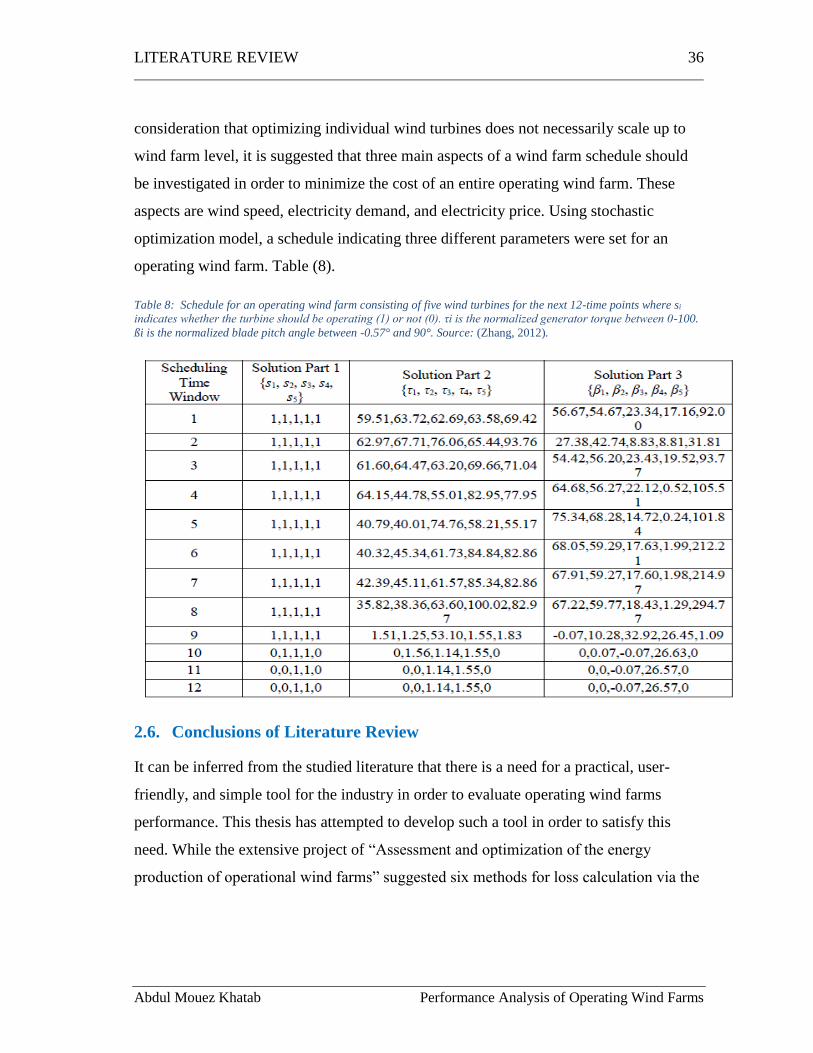
Abdul Mouez Khatab Performance Analysis of Operating Wind Farms
consideration that optimizing individual wind turbines does not necessarily scale up to
wind farm level, it is suggested that three main aspects of a wind farm schedule should
be investigated in order to minimize the cost of an entire operating wind farm. These
aspects are wind speed, electricity demand, and electricity price. Using stochastic
optimization model, a schedule indicating three different parameters were set for an
operating wind farm. Table (8).
Table 8: Schedule for an operating wind farm consisting of five wind turbines for the next 12-time points where si
indicates whether the turbine should be operating (1) or not (0). τi is the normalized generator torque between 0-100.
ßi is the normalized blade pitch angle between -0.57° and 90°. Source: (Zhang, 2012).
2.6. Conclusions of Literature Review
It can be inferred from the studied literature that there is a need for a practical, user-
friendly, and simple tool for the industry in order to evaluate operating wind farms
performance. This thesis has attempted to develop such a tool in order to satisfy this
need. While the extensive project of “Assessment and optimization of the energy
production of operational wind farms” suggested six methods for loss calculation via the

LITERATURE REVIEW 37
Abdul Mouez Khatab Performance Analysis of Operating Wind Farms
use of SCADA system, this thesis will combine two methods to overcome the
weaknesses related to utilizing one of them.
METHODOLOGY 38
Abdul Mouez Khatab Performance Analysis of Operating Wind Farms
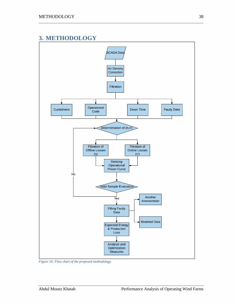
3. METHODOLOGY
Figure 16: Flow chart of the proposed methodology.
METHODOLOGY 39
Abdul Mouez Khatab Performance Analysis of Operating Wind Farms
The followed methodology is depicted in the flow chart above, Figure (16). It starts with
correction of air density aiming to accurately infer the operational power curve.
However, this was not possible for the proposed case study due to lack of reliable source
of pressure and temperature. After that, several filtrations are applied. The filtration
phases can be split into first and second filtration with determination of (n,n’) parameters
in-between, see below
• First filtration phase
It includes removal of the following data:
Firstly, removing all the occurrences where the SCADA system indicates an alarm
code. All the data within the time window between the error start and end times are
removed. Secondly, all the readings with zero or negative power output higher than a
specific wind speed (mainly cut-in speed), i.e. the turbine is not producing were
filtered; these points represent the down time of the wind farm. Thirdly, all events
which are curtailed. Whether the curtailment is intendent or not. Fourthly, all the
faulty logs in the SCADA system were filtered. Faulty logs are events where the record
is missing at either wind speed or power value. These events cannot contribute to the
evaluation and hence are filtered.
• Determination of (n.n’) parameters
After that, the remaining events are divided into wind speed bins in order to calculate
the average and standard deviation of power output at each bin. The average and
standard deviation of the power are interpolated for the entire sample. At this point,
three tools are used to determine the parameters of (n,n’) . These tools are value of the
relative standard deviation representing the spread of the sample, ratio of the filtered
events to the total number of events so far, and visual inspection.
The two parameters defined by (n,n’) have two different objectives. They are used to
identify two different type of associated losses. These two types of losses are online
and offline loss and believed to have different reasons. While (n) is a multiple of the
standard deviation that functions as threshold power curve for detection of offline loss,
(n’) is a multiple of standard deviation that functions as threshold power curve for

METHODOLOGY 40
Abdul Mouez Khatab Performance Analysis of Operating Wind Farms
detection of underperformance related events. In other words, all points that are
deviating more than (n x standard deviation) from the average power value of the bin
are marked as offline loss. Similarly, the points deviating more than (n’ x standard
deviation) from the average power value of the bin are marked as online loss.
• Second filtration
Based on the (n,n’) parameters, all the points deviating more or less than
(n,n’)×standard deviation from the average power value of each bin will be filtered.
The points located below (n,n’)×standard deviation from the average power value of
each bin are considered to be offline- and online losses respectively, more details on
this are found below. On the other hand, the points located above the average power
value of each bin are not considered to be losses. However, they will not contribute to
the construction of the power curve since they represent abnormal operational status.
• Power Curve Calculation
Using the non-parametric binning method, the creation of a representative operational
power curve is done including only the remaining points by using the average power
value per bin vs bin center as wind speed.
• Valid Sample Evaluation
At this point, the term “valid sample” represents the points which will be expected to
have their own power output. This includes the points utilized in the creation of the
operational power curve in addition to the points representing abnormal operational
status and located above the obtained power curve and mentioned above. This is
because the wind turbine will not produce a higher output than its generator’s capacity
at a specific wind speed. This “valid sample” will be evaluated in terms of relative
standard deviation of power output, visual inspection (taking sample points one-by-
one), and ratio of filtered events to the total number of events in order to assess the data
discrepancy which indicates performance behavior of a wind turbine. At this point, a
judgement regarding the selection of the values of (n,n’) is done. If the data is still
exhibiting high discrepancy and/or if the remained points are too few, new values of
METHODOLOGY 41
Abdul Mouez Khatab Performance Analysis of Operating Wind Farms
(n,n’) shall be implemented again. The entire process after determination of (n,n’)
should be re-executed until reaching a satisfactory values of (n,n’).
• Faulty Logs Replacement
In order to precisely assess the performance of a wind turbine and quantify the losses,
all the faulty data in the SCADA system, mainly wind speed readings, need to be
replaced with a representative data for the same time stamp. This is of great importance
for the estimation of the potential energy representing one complete year. Replacement
of faulty wind speed data is done using another anemometer in the wind farm in
ascending order based on the correlation factor. When the entire wind farm exhibits
faulty data, modeled WRF data in one-hour interval is used for the replacement.
Aiming to reduce the uncertainty, WRF data was interpolated to ten-minute interval.
For instance, if Turbine #02 in a given wind farm lacks the wind speed record for a
specific timestamp, this reading will be acquired according to the correlation equation
from the wind turbine which has the highest correlation coefficient; if the data is
missing at that turbine as well, then data from the next highest correlation coefficient is
chosen, and so on until the entire park is examined and the reading is missing from the
entire park. At this point, WRF modeled data is used in sector wise wind speed
correlation in order to withstand wake effects which modeled data does not consider.
In regard to faulty power logs, the creation of a power ratio matrix will lead to
compensation of missing records of power output. However, this is not doable for wind
farms where the entire park would be affected. Another way to compensate for power
records is by checking the injection point where the wind farm feeds the grid.
• Potential Energy and Loss Calculation
At this point, the potential energy can be calculated for the time stamps associated to
losses using the operational power curve as a reference. Points belonging to the valid
sample have the potential energy equal to the actual power output as they are not
associated to losses. Production loss is introduced to assess the performance of
different wind turbines. It should be noted here that production loss value already
considers wake loss and electrical loss since it is based on SCADA data. Equation (4)

METHODOLOGY 42
Abdul Mouez Khatab Performance Analysis of Operating Wind Farms
𝑃𝑟𝑜𝑑𝑢𝑐𝑡𝑖𝑜𝑛 𝐿𝑜𝑠𝑠 =𝐸𝑛𝑒𝑟𝑔𝑦 𝐿𝑜𝑠𝑠
𝑃𝑜𝑡𝑒𝑛𝑡𝑖𝑎𝑙 𝐸𝑛𝑒𝑟𝑔𝑦
Equation 4: Production loss equation.
Where Energy Loss is calculated separately with the help of the applied filtration
criteria, losses include the two main categories offline and online losses as follows:
1. Offline losses
This category includes all losses when the turbine is not expected to be in full
performance, namely operational alarm code, down time, curtailment, icing, and
others. This includes a number of subcategories:
1.1 Operational Alarm code
The operational alarm system flags events where the turbine is not in full performance
due to some reason. Most of the operational alarm systems cover a variety of reasons.
This can be of great help in order to evaluate the reasons standing for losses and, hence,
determining the best measures for optimization.
1.2 Down Time
This category includes points where the turbine has zero or negative power output
though it is expected to have a positive power output. Even though the operational alarm
system is expected to capture these events, it may sometimes fail in this. That is why this
criterion was introduced. Theoretically, this will include wind speeds larger than cut in
speed. However, in practice, this is not necessarily the case due to shifts in the nacelle
transfer function. This category is associated to the availability of the wind turbine.
1.3 Faulty Logs
The SCADA system records a number of faulty data due to various reasons such as
sensor failure. These data are invalid for the creation of the operational power curve.
After substituting these readings, the losses associated to the inserted data are detected
and quantified. It should be noted that losses resulting in this group can be due to a

METHODOLOGY 43
Abdul Mouez Khatab Performance Analysis of Operating Wind Farms
number of reasons such as icing, down time, or underperformance. However, they will
be treated separately due to the higher uncertainty they exhibit. This includes two
subcategories:
Faulty readings in power output: These events lack power output values.
Faulty readings in wind speed: These points lack wind speed values.
1.4 Other Offline Losses
This includes points deviating more than n standard deviations from the mean power
value of a reference bin and that do not belong to the aforementioned categories, i.e. not
flagged by alarm code, not a down time event or a faulty log. These points are
statistically classified as outliers where the turbine significantly produces below the rated
power. They usually represent icing condition or severe loss events.
2 Online Losses
Those are the points deviating between (n) and (n`) from the mean value. They are
associated to turbine underperformance where the turbine is expected to be in full
performance though it is not. Main causes of online losses were described in Section
2.4.2.
Eventually, the aggregate losses are calculated and the main reasons behind losses are
detected, which suggests measures to optimize the performance of the wind farm.
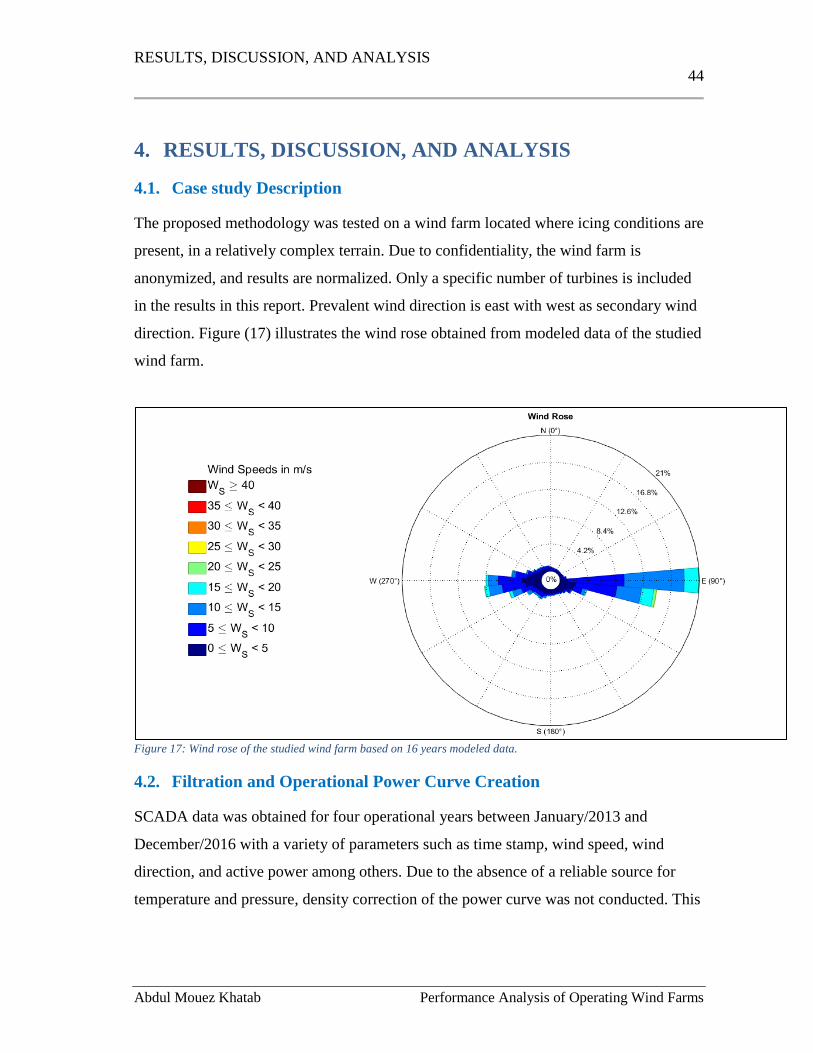
RESULTS, DISCUSSION, AND ANALYSIS
44
Abdul Mouez Khatab Performance Analysis of Operating Wind Farms
4. RESULTS, DISCUSSION, AND ANALYSIS
4.1. Case study Description
The proposed methodology was tested on a wind farm located where icing conditions are
present, in a relatively complex terrain. Due to confidentiality, the wind farm is
anonymized, and results are normalized. Only a specific number of turbines is included
in the results in this report. Prevalent wind direction is east with west as secondary wind
direction. Figure (17) illustrates the wind rose obtained from modeled data of the studied
wind farm.
Figure 17: Wind rose of the studied wind farm based on 16 years modeled data.
4.2. Filtration and Operational Power Curve Creation
SCADA data was obtained for four operational years between January/2013 and
December/2016 with a variety of parameters such as time stamp, wind speed, wind
direction, and active power among others. Due to the absence of a reliable source for
temperature and pressure, density correction of the power curve was not conducted. This
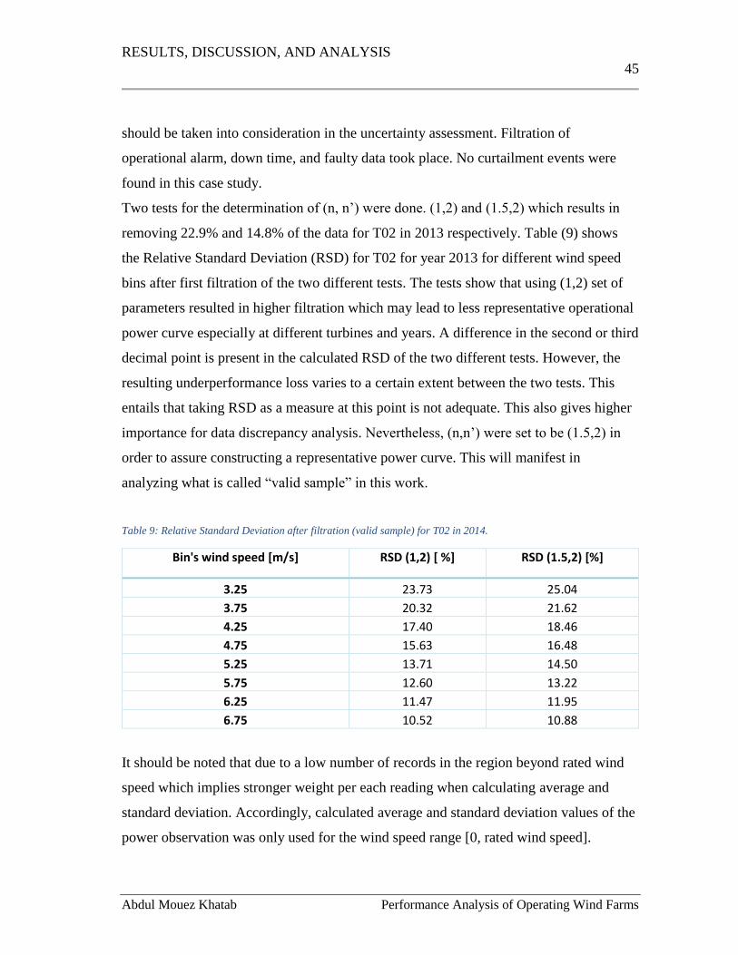
RESULTS, DISCUSSION, AND ANALYSIS
45
Abdul Mouez Khatab Performance Analysis of Operating Wind Farms
should be taken into consideration in the uncertainty assessment. Filtration of
operational alarm, down time, and faulty data took place. No curtailment events were
found in this case study.
Two tests for the determination of (n, n’) were done. (1,2) and (1.5,2) which results in
removing 22.9% and 14.8% of the data for T02 in 2013 respectively. Table (9) shows
the Relative Standard Deviation (RSD) for T02 for year 2013 for different wind speed
bins after first filtration of the two different tests. The tests show that using (1,2) set of
parameters resulted in higher filtration which may lead to less representative operational
power curve especially at different turbines and years. A difference in the second or third
decimal point is present in the calculated RSD of the two different tests. However, the
resulting underperformance loss varies to a certain extent between the two tests. This
entails that taking RSD as a measure at this point is not adequate. This also gives higher
importance for data discrepancy analysis. Nevertheless, (n,n’) were set to be (1.5,2) in
order to assure constructing a representative power curve. This will manifest in
analyzing what is called “valid sample” in this work.
Table 9: Relative Standard Deviation after filtration (valid sample) for T02 in 2014.
Bin's wind speed [m/s] RSD (1,2) [ %] RSD (1.5,2) [%]
3.25 23.73 25.04
3.75 20.32 21.62
4.25 17.40 18.46
4.75 15.63 16.48
5.25 13.71 14.50
5.75 12.60 13.22
6.25 11.47 11.95
6.75 10.52 10.88
It should be noted that due to a low number of records in the region beyond rated wind
speed which implies stronger weight per each reading when calculating average and
standard deviation. Accordingly, calculated average and standard deviation values of the
power observation was only used for the wind speed range [0, rated wind speed].
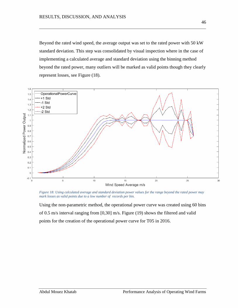
RESULTS, DISCUSSION, AND ANALYSIS
46
Abdul Mouez Khatab Performance Analysis of Operating Wind Farms
Beyond the rated wind speed, the average output was set to the rated power with 50 kW
standard deviation. This step was consolidated by visual inspection where in the case of
implementing a calculated average and standard deviation using the binning method
beyond the rated power, many outliers will be marked as valid points though they clearly
represent losses, see Figure (18).
Figure 18: Using calculated average and standard deviation power values for the range beyond the rated power may
mark losses as valid points due to a low number of records per bin.
Using the non-parametric method, the operational power curve was created using 60 bins
of 0.5 m/s interval ranging from [0,30] m/s. Figure (19) shows the filtered and valid
points for the creation of the operational power curve for T05 in 2016.
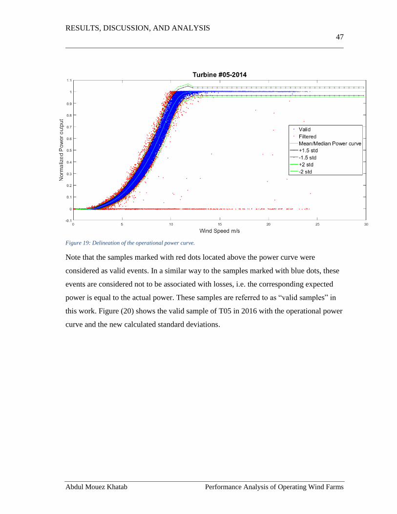
RESULTS, DISCUSSION, AND ANALYSIS
47
Abdul Mouez Khatab Performance Analysis of Operating Wind Farms
Figure 19: Delineation of the operational power curve.
Note that the samples marked with red dots located above the power curve were
considered as valid events. In a similar way to the samples marked with blue dots, these
events are considered not to be associated with losses, i.e. the corresponding expected
power is equal to the actual power. These samples are referred to as “valid samples” in
this work. Figure (20) shows the valid sample of T05 in 2016 with the operational power
curve and the new calculated standard deviations.
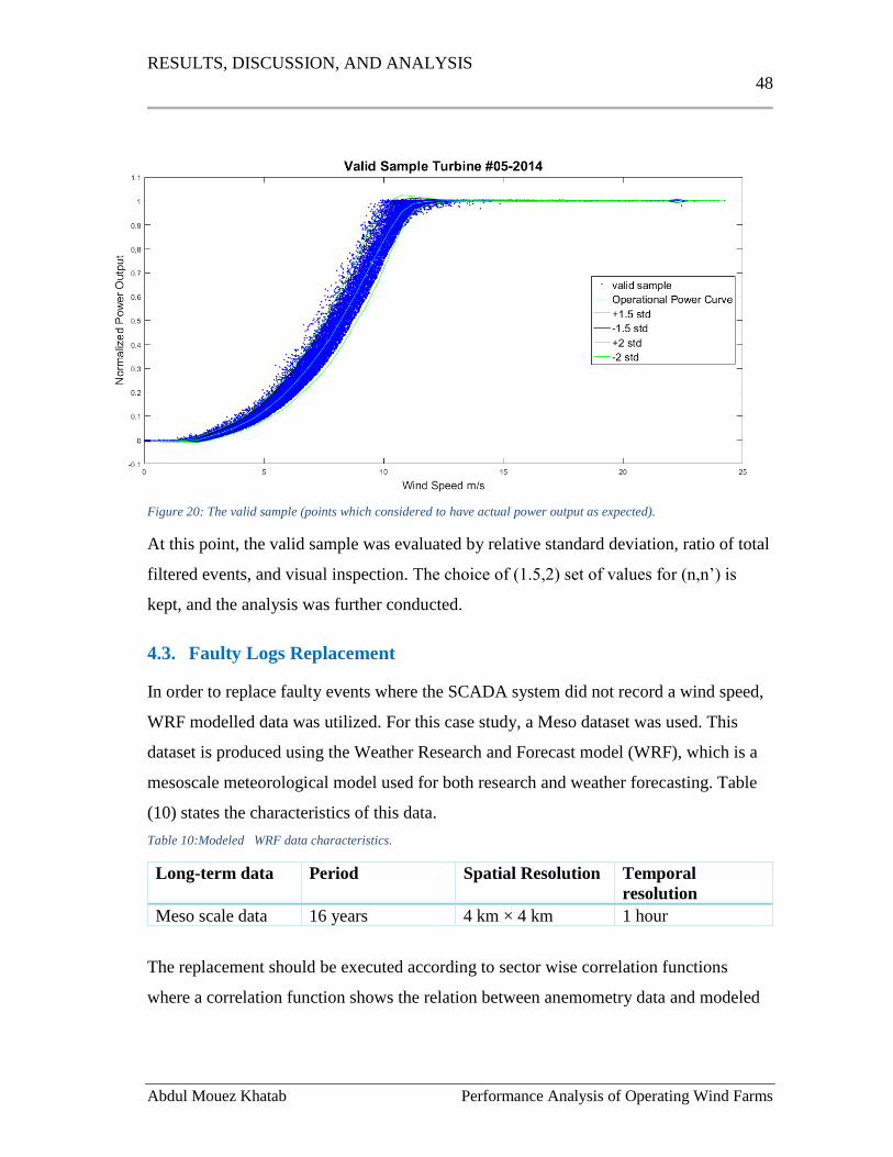
RESULTS, DISCUSSION, AND ANALYSIS
48
Abdul Mouez Khatab Performance Analysis of Operating Wind Farms
Figure 20: The valid sample (points which considered to have actual power output as expected).
At this point, the valid sample was evaluated by relative standard deviation, ratio of total
filtered events, and visual inspection. The choice of (1.5,2) set of values for (n,n’) is
kept, and the analysis was further conducted.
4.3. Faulty Logs Replacement
In order to replace faulty events where the SCADA system did not record a wind speed,
WRF modelled data was utilized. For this case study, a Meso dataset was used. This
dataset is produced using the Weather Research and Forecast model (WRF), which is a
mesoscale meteorological model used for both research and weather forecasting. Table
(10) states the characteristics of this data.
Table 10:Modeled WRF data characteristics.
Long-term data Period Spatial Resolution Temporal
resolution
Meso scale data 16 years 4 km × 4 km 1 hour
The replacement should be executed according to sector wise correlation functions
where a correlation function shows the relation between anemometry data and modeled
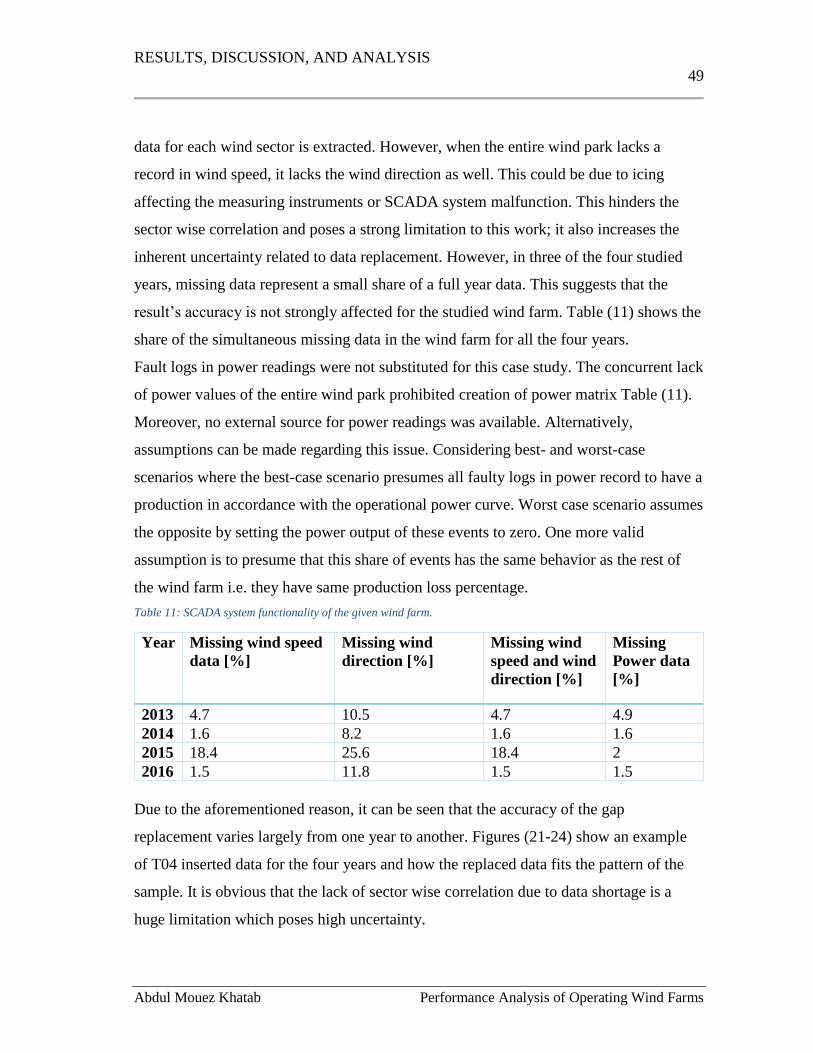
RESULTS, DISCUSSION, AND ANALYSIS
49
Abdul Mouez Khatab Performance Analysis of Operating Wind Farms
data for each wind sector is extracted. However, when the entire wind park lacks a
record in wind speed, it lacks the wind direction as well. This could be due to icing
affecting the measuring instruments or SCADA system malfunction. This hinders the
sector wise correlation and poses a strong limitation to this work; it also increases the
inherent uncertainty related to data replacement. However, in three of the four studied
years, missing data represent a small share of a full year data. This suggests that the
result’s accuracy is not strongly affected for the studied wind farm. Table (11) shows the
share of the simultaneous missing data in the wind farm for all the four years.
Fault logs in power readings were not substituted for this case study. The concurrent lack
of power values of the entire wind park prohibited creation of power matrix Table (11).
Moreover, no external source for power readings was available. Alternatively,
assumptions can be made regarding this issue. Considering best- and worst-case
scenarios where the best-case scenario presumes all faulty logs in power record to have a
production in accordance with the operational power curve. Worst case scenario assumes
the opposite by setting the power output of these events to zero. One more valid
assumption is to presume that this share of events has the same behavior as the rest of
the wind farm i.e. they have same production loss percentage.
Table 11: SCADA system functionality of the given wind farm.
Year Missing wind speed
data [%]
Missing wind
direction [%]
Missing wind
speed and wind
direction [%]
Missing
Power data
[%]
2013 4.7 10.5 4.7 4.9
2014 1.6 8.2 1.6 1.6
2015 18.4 25.6 18.4 2
2016 1.5 11.8 1.5 1.5
Due to the aforementioned reason, it can be seen that the accuracy of the gap
replacement varies largely from one year to another. Figures (21-24) show an example
of T04 inserted data for the four years and how the replaced data fits the pattern of the
sample. It is obvious that the lack of sector wise correlation due to data shortage is a
huge limitation which poses high uncertainty.

RESULTS, DISCUSSION, AND ANALYSIS
50
Abdul Mouez Khatab Performance Analysis of Operating Wind Farms
Figure 21: Data compensation quality for T04 in 2013.
Figure 22: Data compensation quality of T04 in 2014.
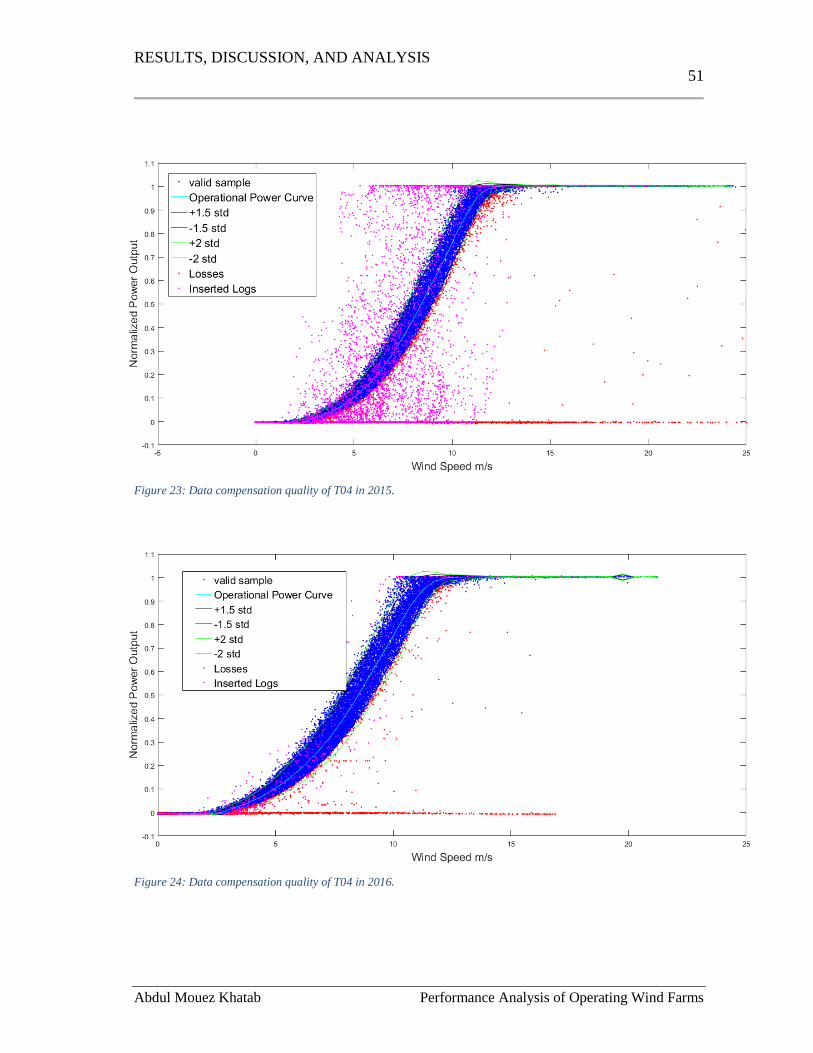
RESULTS, DISCUSSION, AND ANALYSIS
51
Abdul Mouez Khatab Performance Analysis of Operating Wind Farms
Figure 23: Data compensation quality of T04 in 2015.
Figure 24: Data compensation quality of T04 in 2016.
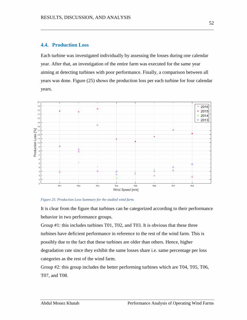
RESULTS, DISCUSSION, AND ANALYSIS
52
Abdul Mouez Khatab Performance Analysis of Operating Wind Farms
4.4. Production Loss
Each turbine was investigated individually by assessing the losses during one calendar
year. After that, an investigation of the entire farm was executed for the same year
aiming at detecting turbines with poor performance. Finally, a comparison between all
years was done. Figure (25) shows the production loss per each turbine for four calendar
years.
Figure 25: Production Loss Summary for the studied wind farm.
It is clear from the figure that turbines can be categorized according to their performance
behavior in two performance groups.
Group #1: this includes turbines T01, T02, and T03. It is obvious that these three
turbines have deficient performance in reference to the rest of the wind farm. This is
possibly due to the fact that these turbines are older than others. Hence, higher
degradation rate since they exhibit the same losses share i.e. same percentage per loss
categories as the rest of the wind farm.
Group #2: this group includes the better performing turbines which are T04, T05, T06,
T07, and T08.
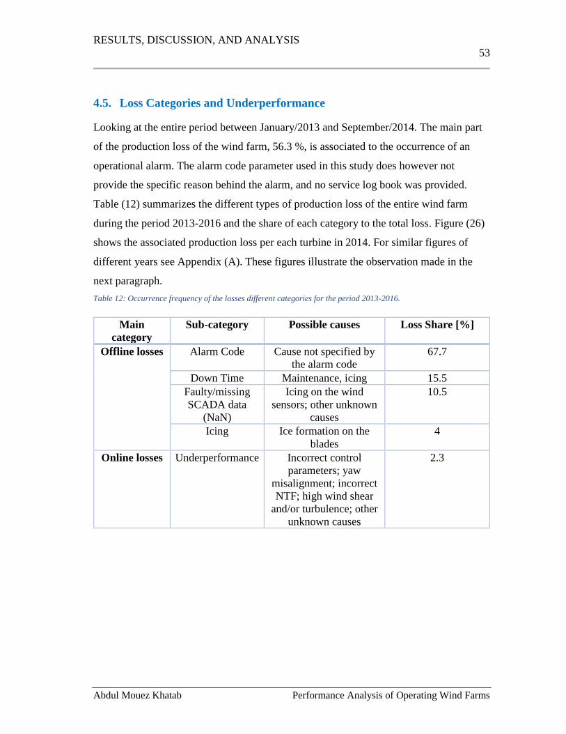
RESULTS, DISCUSSION, AND ANALYSIS
53
Abdul Mouez Khatab Performance Analysis of Operating Wind Farms
4.5. Loss Categories and Underperformance
Looking at the entire period between January/2013 and September/2014. The main part
of the production loss of the wind farm, 56.3 %, is associated to the occurrence of an
operational alarm. The alarm code parameter used in this study does however not
provide the specific reason behind the alarm, and no service log book was provided.
Table (12) summarizes the different types of production loss of the entire wind farm
during the period 2013-2016 and the share of each category to the total loss. Figure (26)
shows the associated production loss per each turbine in 2014. For similar figures of
different years see Appendix (A). These figures illustrate the observation made in the
next paragraph.
Table 12: Occurrence frequency of the losses different categories for the period 2013-2016.
Main
category
Sub-category Possible causes Loss Share [%]
Offline losses Alarm Code Cause not specified by
the alarm code
67.7
Down Time Maintenance, icing 15.5
Faulty/missing
SCADA data
(NaN)
Icing on the wind
sensors; other unknown
causes
10.5
Icing Ice formation on the
blades
4
Online losses Underperformance Incorrect control
parameters; yaw
misalignment; incorrect
NTF; high wind shear
and/or turbulence; other
unknown causes
2.3
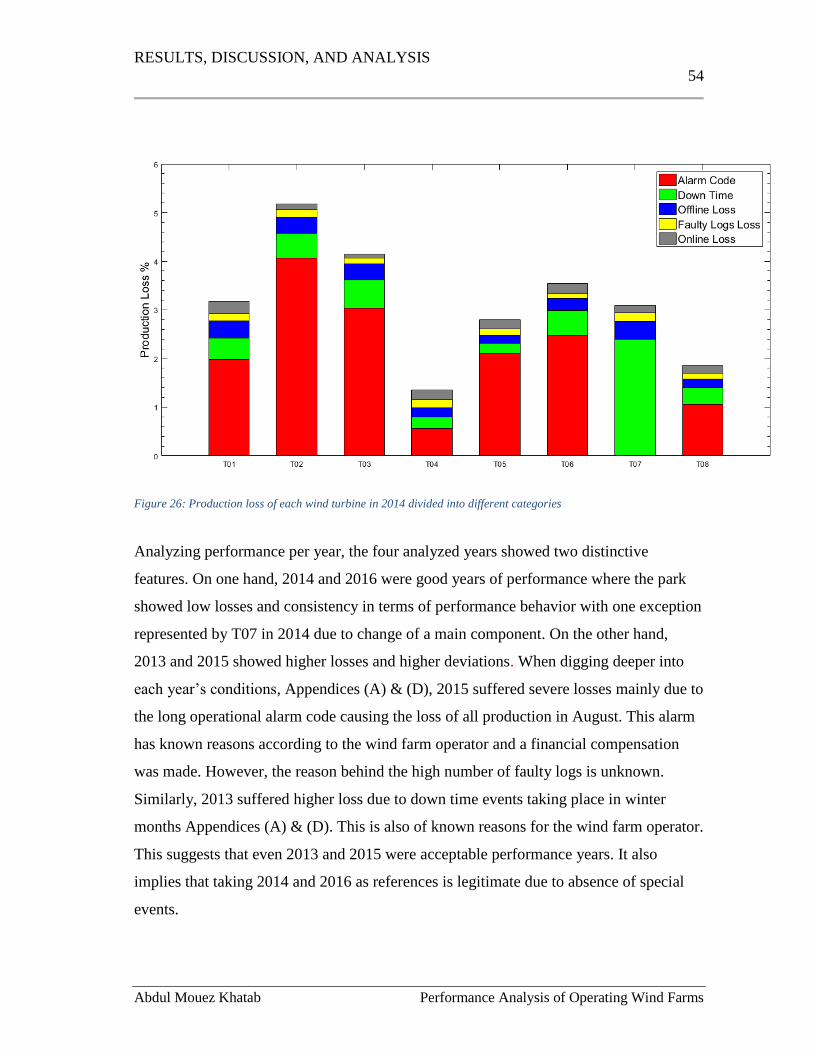
RESULTS, DISCUSSION, AND ANALYSIS
54
Abdul Mouez Khatab Performance Analysis of Operating Wind Farms
Figure 26: Production loss of each wind turbine in 2014 divided into different categories
Analyzing performance per year, the four analyzed years showed two distinctive
features. On one hand, 2014 and 2016 were good years of performance where the park
showed low losses and consistency in terms of performance behavior with one exception
represented by T07 in 2014 due to change of a main component. On the other hand,
2013 and 2015 showed higher losses and higher deviations. When digging deeper into
each year’s conditions, Appendices (A) & (D), 2015 suffered severe losses mainly due to
the long operational alarm code causing the loss of all production in August. This alarm
has known reasons according to the wind farm operator and a financial compensation
was made. However, the reason behind the high number of faulty logs is unknown.
Similarly, 2013 suffered higher loss due to down time events taking place in winter
months Appendices (A) & (D). This is also of known reasons for the wind farm operator.
This suggests that even 2013 and 2015 were acceptable performance years. It also
implies that taking 2014 and 2016 as references is legitimate due to absence of special
events.
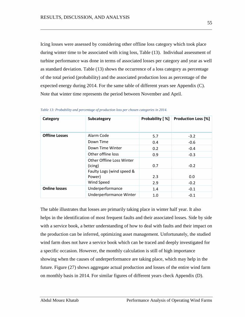
RESULTS, DISCUSSION, AND ANALYSIS
55
Abdul Mouez Khatab Performance Analysis of Operating Wind Farms
Icing losses were assessed by considering other offline loss category which took place
during winter time to be associated with icing loss, Table (13). Individual assessment of
turbine performance was done in terms of associated losses per category and year as well
as standard deviation. Table (13) shows the occurrence of a loss category as percentage
of the total period (probability) and the associated production loss as percentage of the
expected energy during 2014. For the same table of different years see Appendix (C).
Note that winter time represents the period between November and April.
Table 13: Probability and percentage of production loss per chosen categories in 2014.
Category
Subcategory Probability [ %] Production Loss [%]
Offline Losses Alarm Code 5.7 -3.2
Down Time 0.4 -0.6
Down Time Winter 0.2 -0.4
Other offline loss 0.9 -0.3
Other Offline Loss Winter (icing) 0.7 -0.2
Faulty Logs (wind speed & Power) 2.3 0.0
Wind Speed 2.9 -0.2
Online losses
Underperformance 1.4 -0.1
Underperformance Winter 1.0 -0.1
The table illustrates that losses are primarily taking place in winter half year. It also
helps in the identification of most frequent faults and their associated losses. Side by side
with a service book, a better understanding of how to deal with faults and their impact on
the production can be inferred, optimizing asset management. Unfortunately, the studied
wind farm does not have a service book which can be traced and deeply investigated for
a specific occasion. However, the monthly calculation is still of high importance
showing when the causes of underperformance are taking place, which may help in the
future. Figure (27) shows aggregate actual production and losses of the entire wind farm
on monthly basis in 2014. For similar figures of different years check Appendix (D).
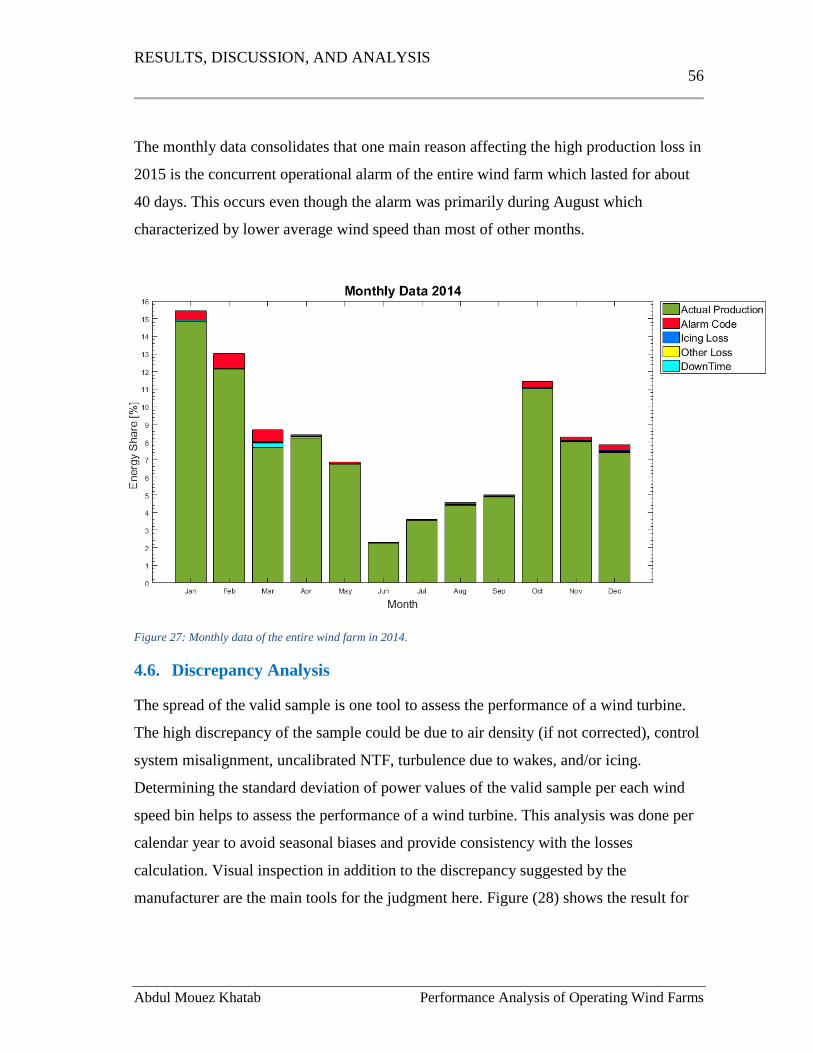
RESULTS, DISCUSSION, AND ANALYSIS
56
Abdul Mouez Khatab Performance Analysis of Operating Wind Farms
The monthly data consolidates that one main reason affecting the high production loss in
2015 is the concurrent operational alarm of the entire wind farm which lasted for about
40 days. This occurs even though the alarm was primarily during August which
characterized by lower average wind speed than most of other months.
Figure 27: Monthly data of the entire wind farm in 2014.
4.6. Discrepancy Analysis
The spread of the valid sample is one tool to assess the performance of a wind turbine.
The high discrepancy of the sample could be due to air density (if not corrected), control
system misalignment, uncalibrated NTF, turbulence due to wakes, and/or icing.
Determining the standard deviation of power values of the valid sample per each wind
speed bin helps to assess the performance of a wind turbine. This analysis was done per
calendar year to avoid seasonal biases and provide consistency with the losses
calculation. Visual inspection in addition to the discrepancy suggested by the
manufacturer are the main tools for the judgment here. Figure (28) shows the result for
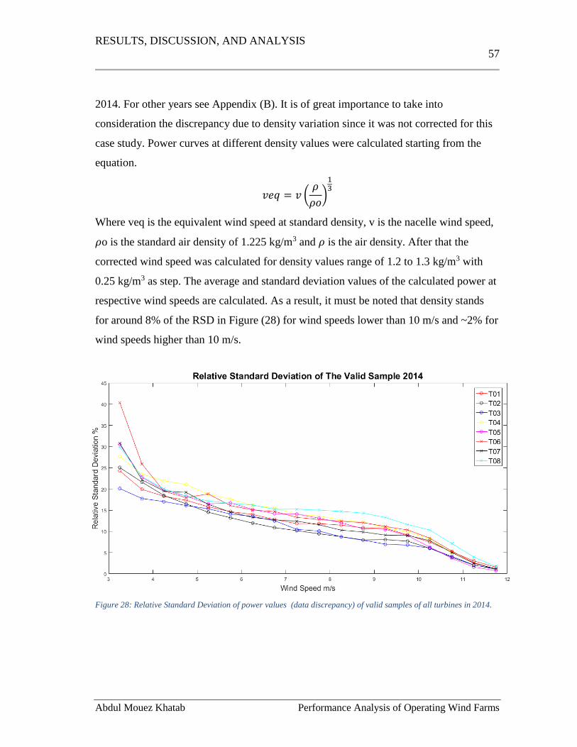
RESULTS, DISCUSSION, AND ANALYSIS
57
Abdul Mouez Khatab Performance Analysis of Operating Wind Farms
2014. For other years see Appendix (B). It is of great importance to take into
consideration the discrepancy due to density variation since it was not corrected for this
case study. Power curves at different density values were calculated starting from the
equation.
𝑣𝑒𝑞 = 𝑣 (𝜌
𝜌𝑜)
13
Where veq is the equivalent wind speed at standard density, v is the nacelle wind speed,
𝜌o is the standard air density of 1.225 kg/m3 and 𝜌 is the air density. After that the
corrected wind speed was calculated for density values range of 1.2 to 1.3 kg/m3 with
0.25 kg/m3 as step. The average and standard deviation values of the calculated power at
respective wind speeds are calculated. As a result, it must be noted that density stands
for around 8% of the RSD in Figure (28) for wind speeds lower than 10 m/s and ~2% for
wind speeds higher than 10 m/s.
Figure 28: Relative Standard Deviation of power values (data discrepancy) of valid samples of all turbines in 2014.
RESULTS, DISCUSSION, AND ANALYSIS
58
Abdul Mouez Khatab Performance Analysis of Operating Wind Farms
Looking at Appendix B, it can be seen that the pattern is similar among different years
for turbines like T04 and T08 showing higher discrepancy than the rest of the wind farm.
It is also clear that some turbines discrepancy fluctuates from year to year like T06.
4.7. Optimization Measures
Two measures could be taken into action to reach a better performance of the studied
wind farm.
1. Enhancing data availability in the SCADA system. In order to do this, further
investigation should be conducted to check what is responsible for this; whether
it is SCADA communication system, storage or measuring instrument. It should
be noted when looking at Table (11) that whenever wind speed is missing all
over the park the wind direction is missing as well, though not the power. This
implies that data availability is possibly related to measuring instrument’s
quality. Tackling this issue will provide more information about the causes of
underperformance, hence, better evaluation and measures to improve
performance.
2. Nacelle mounted lidar on one of the turbines showing the highest deviation from
the rest of the wind farm in terms of standard deviation of the valid sample,
namely T08. This will be highly beneficial in determining yaw misalignment
error as well as the right parameters for the NTF.
CONCLUSIONS 59
Abdul Mouez Khatab Performance Analysis of Operating Wind Farms
5. CONCLUSIONS
5.1. Summary of the Work
A practical, easily implemented method was developed for the assessment of wind farm
performance. SCADA data and modeled data are needed for this work. The creation of a
representative operational power curve was done and specific calculations for the
purpose of performance evaluation are executed. The three main questions investigated
in this work were the following:
- To calculate the potential energy output and associated losses.
- To determine the main drivers of loss/underperformance events.
- To suggest appropriate optimization measures.
For the chosen case study, three wind turbines are strongly underperforming in
comparison with the rest of the wind farm. This is most likely due to higher depreciation
since they are older than the rest. Issues related to control systems are also probable
causes of underperformance. The wind direction measurements for some turbines show a
clear offset. It is likely that this fact has no impact on the performance of the turbines
since the yaw of the nacelle is related to changes in the wind direction, rather than the
absolute value of the wind direction measurements. Nevertheless, the high discrepancy
of power vs. wind speed of what is defined as “valid sample” in this work suggests that
control systems contribute to underperformance, also drawing a clear picture of what
turbines are underperforming the most.
5.2. Limitations
Several limitations have been encountered in this work and have led to a less accurate
judgment. The main limitations of this work are as follows:
• Lack of detailed reason behind the alarm. This was a limitation for both the
determination of main causes of loss, and for the suggestion of appropriate
optimization measures.
• Poor data availability of SCADA system data where high percentage of data is
missing. Moreover, the poor correlation of modeled data to the SCADA wind
CONCLUSIONS 60
Abdul Mouez Khatab Performance Analysis of Operating Wind Farms
direction which prevented the sector wise correlation for data compensation. It also
prevented assessing which wind sector contributes mostly to losses.
• The studied wind farm lacked a historical service book, which in turn hinders analysis
and investigation of special cases happened during specific periods.
• Lack of reliable sources for air density corrections as well as power output data at the
grid injection point. This increases the inherent uncertainties related to this work.
5.3. Future Work
The present methodology can be combined with a reassessment of the estimated AEP of
wind farms. Similarly, based on the monthly production, production index on monthly
basis can be created which will help hedging the income of the wind farm by a more
accurate estimation of the monthly production. Also;
• Choosing what type of data is best for data replacement, i.e. modeled data, reanalyzed
data or weather stations.
• Keeping track of what benefits the optimization measure results in terms of financial
income. Thus, will enrich this study.
REFERENCES 61
Abdul Mouez Khatab Performance Analysis of Operating Wind Farms
REFERENCES
Baring-Gould, I., Cattin, R., Durstewitz, M., Hulkkonen, M., Krenn, A., Laakso, T.,
Lacroix, A., Peltola, E., Ronsten, G., Tallhaug, L., Wallenius, T., 2012. Wind
Energy Projects in Cold Climates 1–43.
Bi, R., Zhou, C., Hepburn, D.M., 2016. Detection and classification of faults in pitch-
regulated wind turbine generators using normal behaviour models based on
performance curves. Renew. Energy 105, 674–688.
doi:10.1016/j.renene.2016.12.075
Boden, T.A., Andres, R.J., Marland, G., 2017. Global, Regional, and National Fossil-
Fuel CO2 Emissions. doi:10.3334/CDIAC/00001_V2017
Castellani, F., Astolfi, D., Garinei, A., Proietti, S., Sdringola, P., Terzi, L., Desideri, U.,
2015a. How Wind Turbines Alignment to Wind Direction Affects Efficiency? A
Case Study through SCADA Data Mining. Energy Procedia 75, 697–703.
doi:10.1016/j.egypro.2015.07.495
Castellani, F., Astolfi, D., Sdringola, P., Proietti, S., Terzi, L., 2015b. Analyzing wind
turbine directional behavior: SCADA data mining techniques for efficiency and
power assessment. Appl. Energy 185, 1076–1086.
doi:10.1016/j.apenergy.2015.12.049
Chehouri, A., Younes, R., Ilinca, A., Perron, J., 2015. Review of performance
optimization techniques applied to wind turbines. Appl. Energy 142, 361–388.
doi:10.1016/j.apenergy.2014.12.043
Davis, N.N., Byrkjedal, Ø., Hahmann, A.N., Clausen, N.-E., Žagar Mark, 2015. Ice
detection on wind turbines using the observed power curve. Wind Energy 17.
doi:10.1002/we
Dye, L., 2016. Wind Is Fastest Growing Energy Resource - ABC News.
ECOFYS, 2014. Experience with renewable electricity (RES-E) support schemes in
Euro… [WWW Document]. URL https://www.slideshare.net/Ecofys/ecofys-
2014webinarrese-supportpoliciesineurope (accessed 6.29.17).
ERU Met Data - Wind Turbine Power [WWW Document], 2017. URL
http://www.elm.eru.rl.ac.uk/ins4.html (accessed 10.5.17).
Godwin, J.L., Matthews, P., 2013. Classification and Detection of Wind Turbine Pitch
Faults Through SCADA Data Analysis. Int. J. Progn. Heal. Manag. 4.
Hansson, J., Johannes, L., ØYVIND, B., Kjeller vindteknikk, 2016. Quantification of
icing losses in wind farms.
International Electrotechnical Commission, 2013. International Standard IEC 61400-12-
2.
Kim, H.-W., Ko, K.-N., Huh, J.-C., 2013. Wind Turbine Power Performance Testing
Using Nacelle Transfer Function 33, 51–58.
Klemm, M., 2014. Economic Feasibility of Wind Turbines’ Anti-Icing Systems. J.
REFERENCES 62
Abdul Mouez Khatab Performance Analysis of Operating Wind Farms
Chem. Inf. Model. 0, 63. doi:10.1017/CBO9781107415324.004
Kusiak, A., Verma, A., 2013. Monitoring wind farms with performance curves. IEEE
Trans. Sustain. Energy 4. doi:10.1109/TSTE.2012.2212470
Kusiak, A., Zhang, Z., Li, M., 2010. Optimization of wind turbine performance with
data-driven models. IEEE Trans. Sustain. Energy 1, 66–76.
doi:10.1109/TSTE.2010.2046919
Liléo, S., Berge, E., Undheim, O., Klinkert, R., Rolv, E., Vindteknikk, K., 2013. Long-
term correction of wind measurements Long-term correction of wind measurements
State-of-the-art , guidelines and future work.
Lindvall, J., Hansson, J., Undheim, O., Kjeller vindteknikk, 2016. Post-construction
production assessment of wind farms.
Morton, B., 2013. Understanding Wind Turbine Condition Monitoring Systems.
Nivedh, B.S., 2014. Major Failures in the wind turbine components and the importance
of periodic inspections. Wind Insid.
Nymfa Noppe, 2014. Performance monitoring by tracking estimated power curves on a
wind farm level.
Oh, H., Kim, B., 2015. Comparison and verification of the deviation between guaranteed
and measured wind turbine power performance in complex terrain. Energy 85.
doi:10.1016/j.energy.2015.02.115
Sheng, S., 2013. Report on Wind Turbine Subsystem Reliability - A Survey of Various
Databases. NREL/PR-5000-59111,National Renew. Energy Lab.
Singh, P., 2013. Analytical Techniques of SCADA Data to Assess Operational Wind
Turbine Performance.
Standard Deviation [WWW Document], 2017. URL
http://www.investopedia.com/terms/s/standarddeviation.asp (accessed 9.15.17).
Turkyilmaz, U., Hansson, J., Undehem, O., Kjeller vindteknikk, 2016. Use of remote
sensing for performance optimization of wind farms.
Tücer, R., 2016. Investigation of Potential Reasons to Account for the
Underperformance of an Operational Wind Farm.
United Nations, 2015. Sustainable development goals - United Nations [WWW
Document]. URL http://www.un.org/sustainabledevelopment/sustainable-
development-goals/ (accessed 6.29.17).
What is SCADA? Webopedia Definition [WWW Document], 2017. URL
http://www.webopedia.com/TERM/S/SCADA.html (accessed 9.15.17).
Yang, W., Court, R., Jiang, J., 2013. Wind turbine condition monitoring by the approach
of SCADA data analysis. Renew. Energy 53. doi:10.1016/j.renene.2012.11.030
Zhang, Z., 2012. Performance optimization of wind turbines.
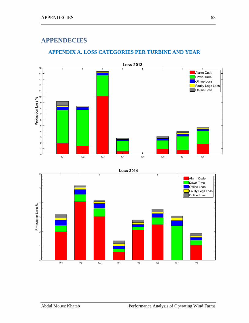
APPENDECIES 63
Abdul Mouez Khatab Performance Analysis of Operating Wind Farms
APPENDECIES
APPENDIX A. LOSS CATEGORIES PER TURBINE AND YEAR
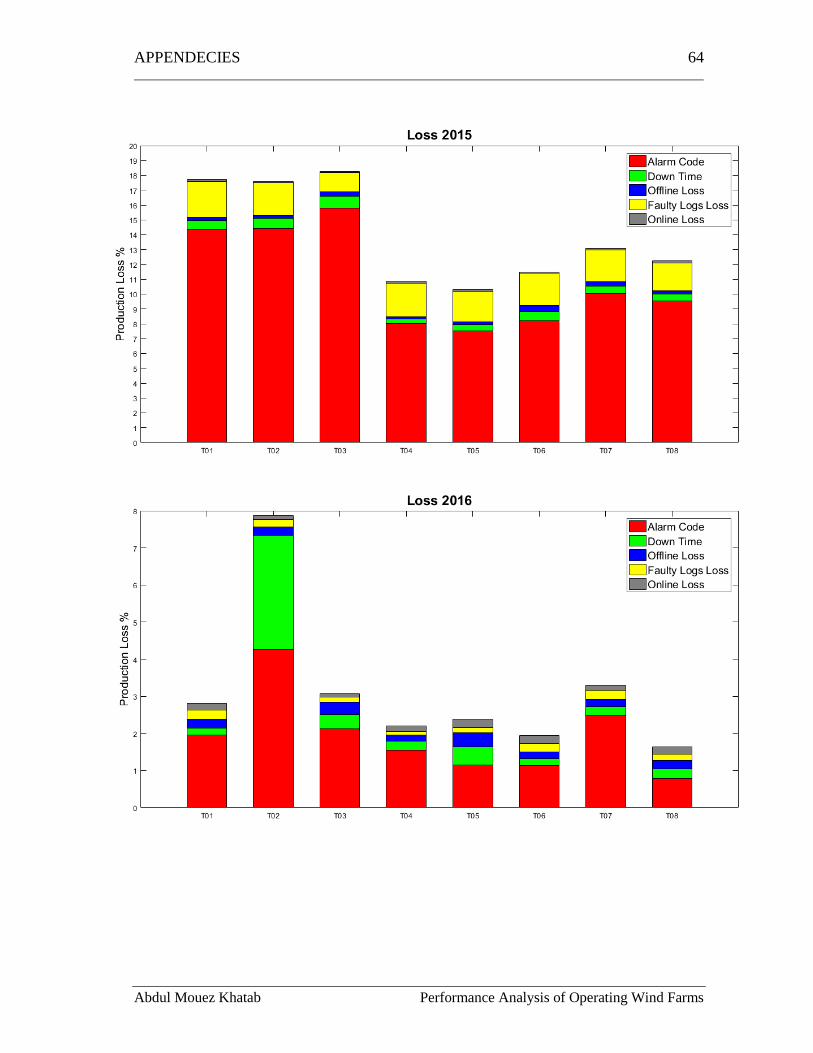
APPENDECIES 64
Abdul Mouez Khatab Performance Analysis of Operating Wind Farms
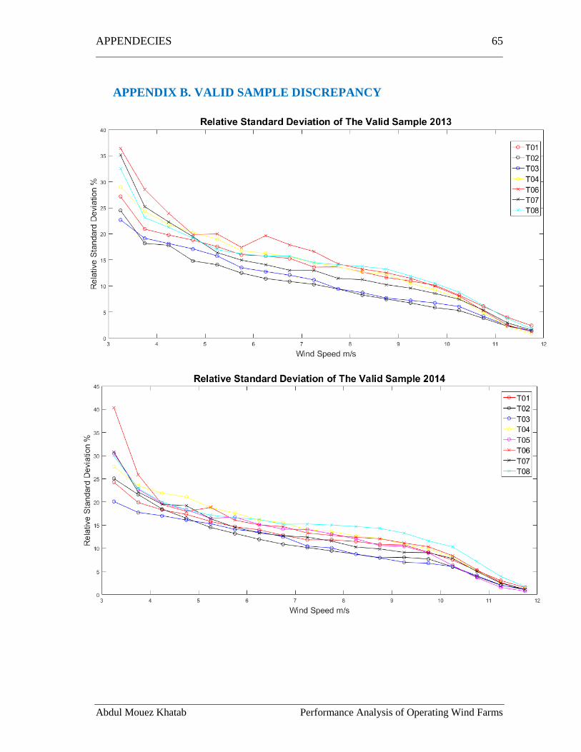
APPENDECIES 65
Abdul Mouez Khatab Performance Analysis of Operating Wind Farms
APPENDIX B. VALID SAMPLE DISCREPANCY
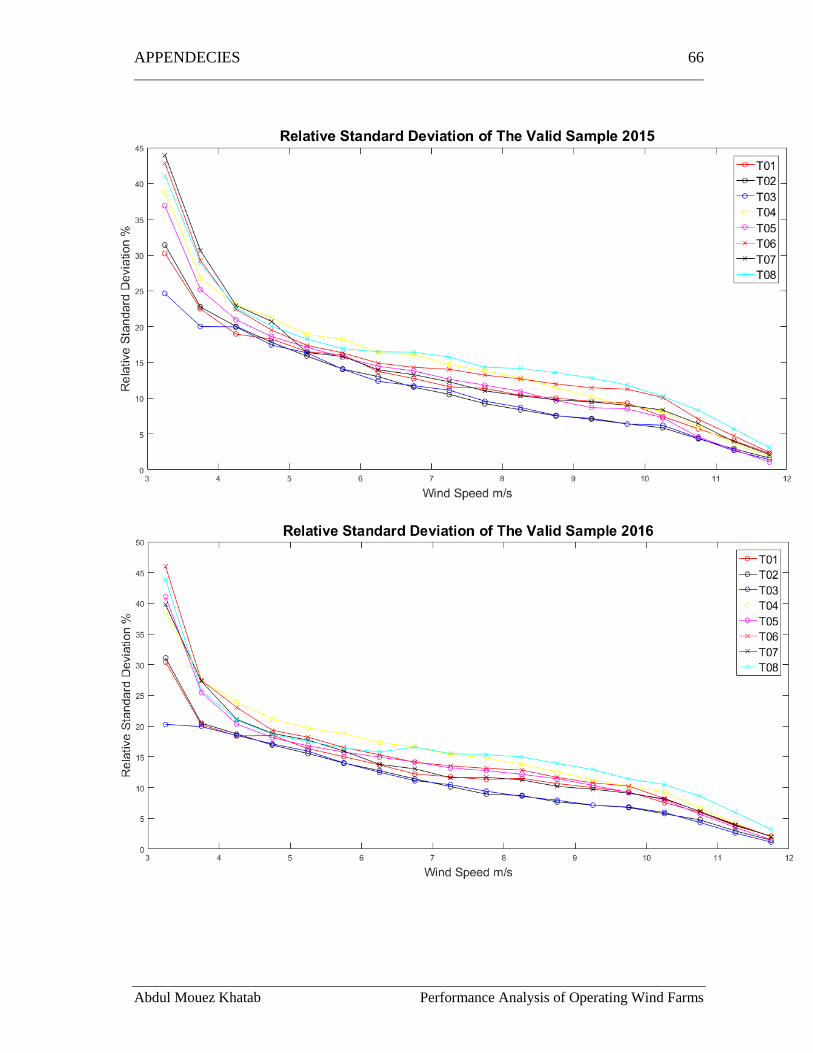
APPENDECIES 66
Abdul Mouez Khatab Performance Analysis of Operating Wind Farms
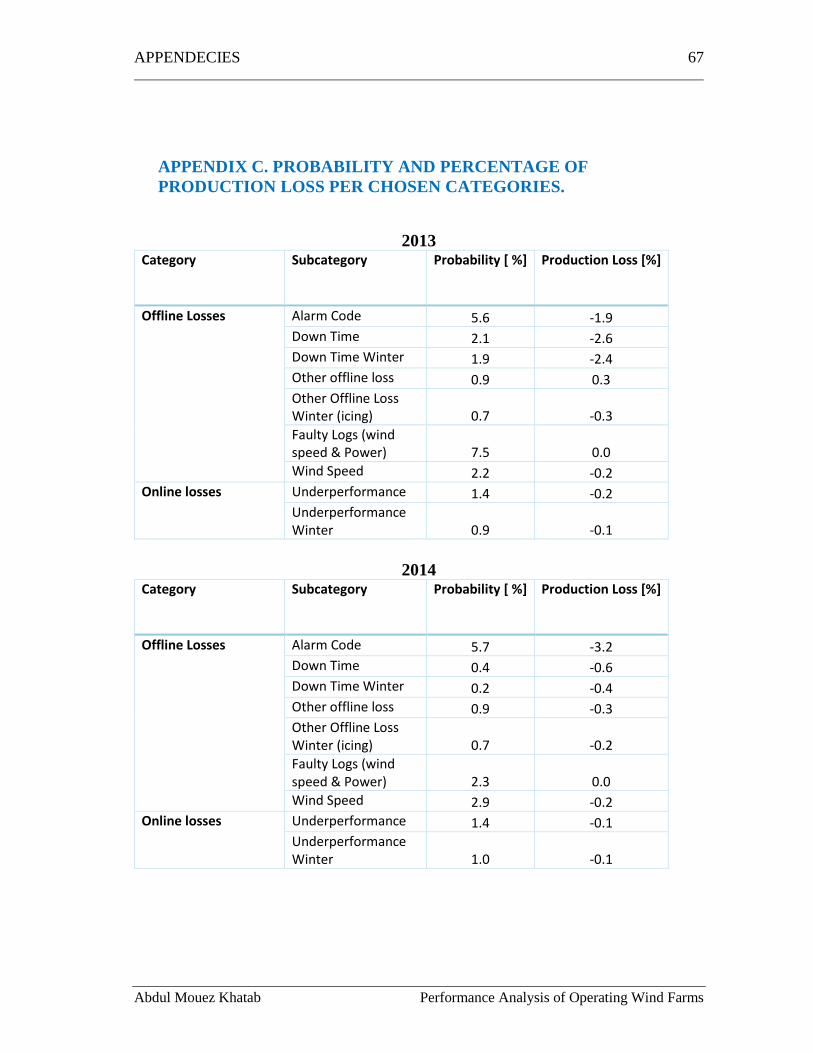
APPENDECIES 67
Abdul Mouez Khatab Performance Analysis of Operating Wind Farms
APPENDIX C. PROBABILITY AND PERCENTAGE OF
PRODUCTION LOSS PER CHOSEN CATEGORIES.
2013 Category
Subcategory Probability [ %] Production Loss [%]
Offline Losses Alarm Code 5.6 -1.9
Down Time 2.1 -2.6
Down Time Winter 1.9 -2.4
Other offline loss 0.9 0.3
Other Offline Loss Winter (icing) 0.7 -0.3
Faulty Logs (wind speed & Power) 7.5 0.0
Wind Speed 2.2 -0.2
Online losses
Underperformance 1.4 -0.2
Underperformance Winter 0.9 -0.1
2014 Category
Subcategory Probability [ %] Production Loss [%]
Offline Losses Alarm Code 5.7 -3.2
Down Time 0.4 -0.6
Down Time Winter 0.2 -0.4
Other offline loss 0.9 -0.3
Other Offline Loss Winter (icing) 0.7 -0.2
Faulty Logs (wind speed & Power) 2.3 0.0
Wind Speed 2.9 -0.2
Online losses
Underperformance 1.4 -0.1
Underperformance Winter 1.0 -0.1
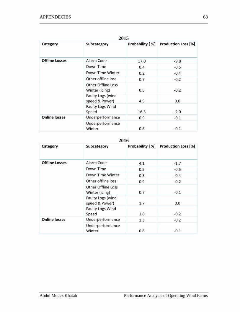
APPENDECIES 68
Abdul Mouez Khatab Performance Analysis of Operating Wind Farms
2015 Category
Subcategory Probability [ %] Production Loss [%]
Offline Losses Alarm Code 17.0 -9.8
Down Time 0.4 -0.5
Down Time Winter 0.2 -0.4
Other offline loss 0.7 -0.2
Other Offline Loss Winter (icing) 0.5 -0.2
Faulty Logs (wind speed & Power) 4.9 0.0
Faulty Logs Wind Speed 16.3 -2.0
Online losses
Underperformance 0.9 -0.1
Underperformance Winter 0.6 -0.1
2016 Category
Subcategory Probability [ %] Production Loss [%]
Offline Losses Alarm Code 4.1 -1.7
Down Time 0.5 -0.5
Down Time Winter 0.3 -0.4
Other offline loss 0.9 -0.2
Other Offline Loss Winter (icing) 0.7 -0.1
Faulty Logs (wind speed & Power) 1.7 0.0
Faulty Logs Wind Speed 1.8 -0.2
Online losses
Underperformance 1.3 -0.2
Underperformance Winter 0.8 -0.1
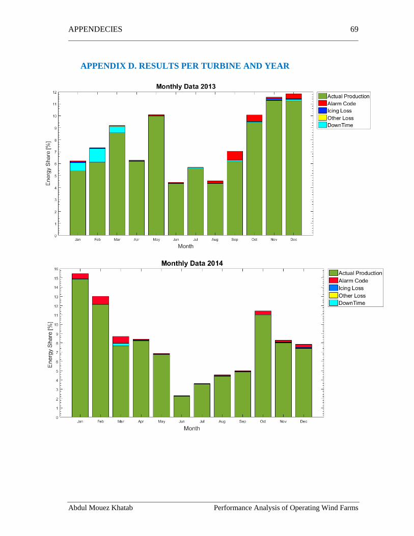
APPENDECIES 69
Abdul Mouez Khatab Performance Analysis of Operating Wind Farms
APPENDIX D. RESULTS PER TURBINE AND YEAR
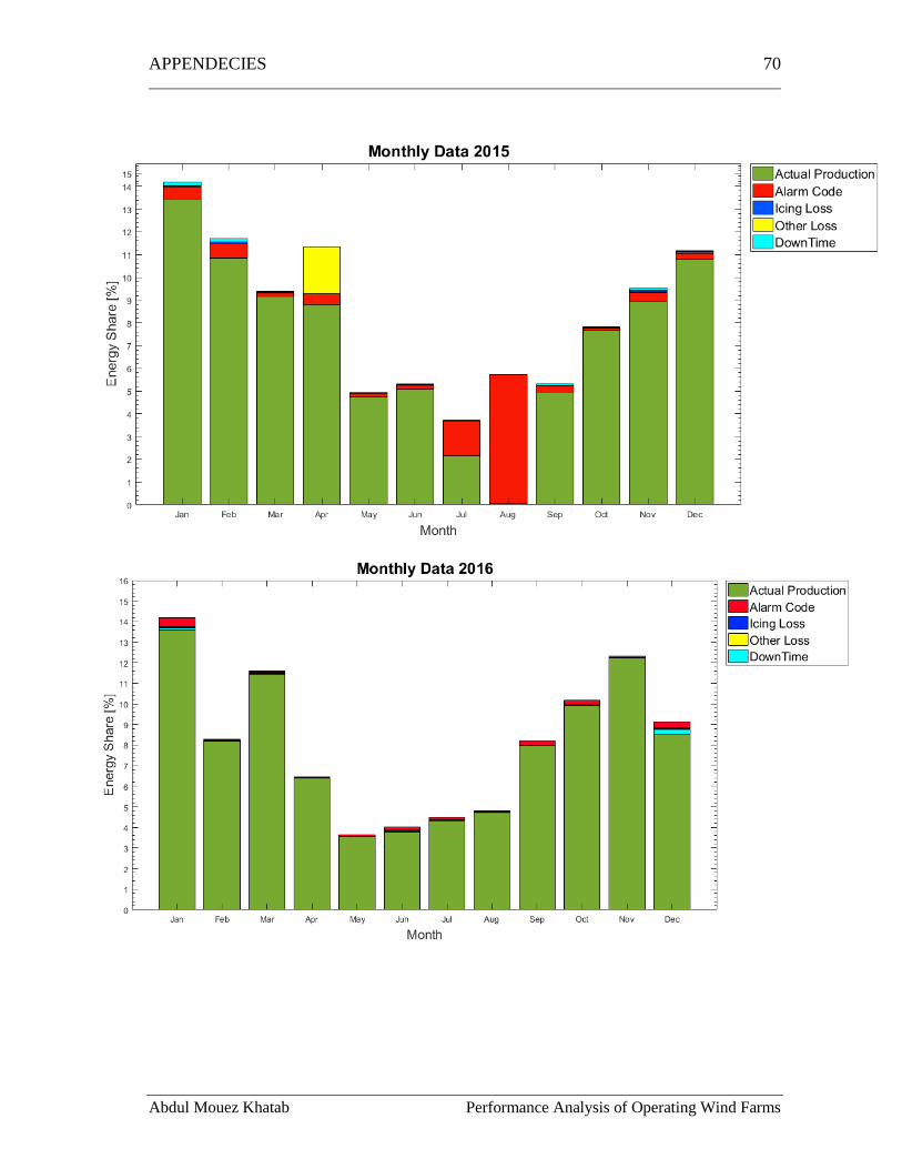
APPENDECIES 70
Abdul Mouez Khatab Performance Analysis of Operating Wind Farms