Performance Analysis of Cooperative Communication for Wireless

Performance Analysis of Cooperative Communication for Wireless Networks

by

Ramesh Chembil Palat

Dissertation submitted to the Faculty of

Virginia Polytechnic Institute and State University

in partial fulfillment of the requirements of the degree of

DOCTOR OF PHILOSOPHY in

Electrical Engineering

Jeffrey H. Reed (Co-chair)

A. Annamalai (Co-Chair)

William H. Tranter

Steven W. Ellingson

Calvin J. Ribbens

December 8, 2006 Blacksburg, Virginia

Keywords: Cooperative Communication, Relaying, MIMO, Wireless Communications

Copyright 2006, Ramesh Chembil Palat

Performance Analysis of Cooperative Communication for Wireless Networks

Ramesh Chembil Palat

Abstract

The demand for access to information when and where you need has motivated the

transition of wireless communications from a fixed infrastructure based cellular

communications technology to a more pervasive adhoc wireless networking technology.

Challenges still remain in wireless adhoc networks in terms of meeting higher capacity

demands, improved reliability and longer connectivity before it becomes a viable

widespread commercial technology. Present day wireless mesh networking uses node-to-

node serial multi-hop communication to convey information from source to destination in

the network. The performance of such a network depends on finding the best possible

route between the source and destination nodes. However the end-to-end performance

can only be as good as the weakest link within a chosen route. Unlike wired networks, the

quality of point-to-point links in a wireless mesh network is subject to random

fluctuations. This adversely affects the performance resulting in poor throughput and

poor energy efficiency.

In recent years, a new paradigm for communication called cooperative communications

has been proposed for which initial information theoretic studies have shown the

potential for improvements in capacity over traditional multi-hop wireless networks.

Cooperative communication involves exploiting the broadcast nature of the wireless

medium to form virtual antenna arrays out of independent single-antenna network nodes

for transmission. In this research we explore the fundamental performance limits of

iii

cooperative communication under more practical operating scenarios. Specifically we

provide a framework for computing the outage and ergodic capacities of non identical

distributed MIMO links, study the effect of time synchronization error on system

performance, analyze the end-to-end average bit error rate (ABER) performance under

imperfect relaying, and study range extension and energy efficiency offered by the

system when compared to a traditional system.

iv

ACKNOWLEDGEMENTS

My sincere appreciation goes to Dr. Jeffrey H. Reed for his valuable guidance, technical

inputs and encouragement throughout my course of study at Virginia Tech. He has

allowed me a free hand in exploring many ideas and I have gained immensely from them.

I would like to express my gratitude to Dr. Annamalai for being a great mentor and for

numerous technical discussions and suggestions that have found their way into this

dissertation. I would also like to thank Dr. William H. Tranter, Dr. Steven S. Ellingson,

and Dr. Calvin J. Ribbens for serving on my committee, for their guidance and criticism

offered.

I would like to acknowledge the support from Wireless @ Virginia Tech industrial

affiliates program and Office of Naval Research for sponsoring this research. I greatly

appreciate the help of the MPRG staff including Shelby Smith, Hilda Reynolds, Jenny

Frank and Cindy Graham for taking excellent care of many of our administrative needs.

This journey towards a PhD would not have been an enjoyable one without the friendship

and assistance from my fellow MPRG students including Ran Gozali, Raqibul Mostafa,

James Hicks, William Newhall, Max Roberts, Srikathyayani Srikanteswara, Carl Dietrich,

Shakheela Marikar, Maruf Mohammad, Jody Neel, Chris Anderson, Yash Vasavada,

Sesh Krishnamoorthy, Anu Hariharan, Jing Jiang, Rekha Menon, Youping Zhao, Kyung

Bae, Swaroop Venkatesh, Jihad Ibrahim, Carlos Aguayo, Philip Balister and Joseph

Gaeddert.

Over the years of my stay in Blacksburg I have been fortunate to have a good network of

friends and especially my roomies Praveen Sheethalnath, Renjith Mathew, Anwar Bashir,

John Korah, Kamesh Chandrasekar, Venkatasubramanian, Vishnu Vimjam and Ravi

v

Shenoy whom I would like to thank for their support and help. I would not have come so

far if it were not for my close friends who have been there for me when I needed them

and who have been a source of encouragement throughout.

I would mostly like to thank my parents, Ramakrishnan Nangali and Rema Chembil Palat,

whose constant and limitless support, motivation, and unwavering belief in me had a

great part in nurturing my dreams and bringing this work to completion.

vi

Table of Contents

1 Introduction and literature survey ..................................................................................................... 1

1.1 Cooperative Communication..................................................................................................... 2 1.2 Literature review ....................................................................................................................... 7 1.3 Key contributions .................................................................................................................... 12 1.4 Organization of thesis.............................................................................................................. 14

2 Outage and ergodic capacities of distributed OSTBC cooperative networks............................... 16

2.1 Generic expressions for the ergodic and outage capacities ..................................................... 17 2.2 Efficient computation of the Bromwich integral..................................................................... 21 2.3 Results ..................................................................................................................................... 24 2.4 Conclusions ............................................................................................................................. 29

3 Efficient Bit Error Rate Analysis of Bandlimited Cooperative OSTBC Networks under Time Synchronization Errors ............................................................................................................................ 30

3.1 System model .......................................................................................................................... 33 3.2 Frequency domain analysis ..................................................................................................... 37 3.3 Extension to distributed 1Ν × MISO networks ....................................................................... 44 3.4 Computational results.............................................................................................................. 46 3.5 Conclusions ............................................................................................................................. 54

4 Node density and range improvement in cooperative networks using randomized STBC ......... 55

4.1 System model .......................................................................................................................... 56 4.2 SINR using Gaussian Approximation ..................................................................................... 59 4.3 Computational results.............................................................................................................. 62 4.4 Conclusions ............................................................................................................................. 65

5 Selective decode and forward cooperative communication under imperfect regeneration......... 66

5.1 System model .......................................................................................................................... 68 5.2 Optimum SNR threshold γ ∗ ................................................................................................... 77 5.3 Energy efficiency of SDF based cooperative communication ................................................ 79 5.4 Computational results and remarks ......................................................................................... 82 5.5 Conclusions ........................................................................................................................... 100

6 Log-Likelihood-Ratio based Selective Decode and Forward Cooperative Communication ..... 102

6.1 Log likelihood criterion......................................................................................................... 102 6.2 ABER performance analysis ................................................................................................. 104 6.3 Optimal LLR threshold ......................................................................................................... 107 6.4 Results ................................................................................................................................... 108 6.5 Conclusions ........................................................................................................................... 110

7 A practical application of cooperative communication: cooperative relaying for ad-hoc ground networks using swarm UAVs................................................................................................................. 111

7.1 Background ........................................................................................................................... 113 7.2 Statistical channel models and path loss exponent for UAV based communication............. 114 7.3 UAV flight characteristics..................................................................................................... 117 7.4 UAV relay based cooperative communication architecture .................................................. 118 7.5 Simulation set-up and results ................................................................................................ 119

vii

7.6 Conclusions ........................................................................................................................... 127

8 Frequency domain based ABER analysis for bandlimited BPSK system with time synchronization error ............................................................................................................................. 129

8.1 System model ........................................................................................................................ 130 8.2 Numerical Results ................................................................................................................. 134 8.3 Conclusions ........................................................................................................................... 137

9 Conclusions and Future Work ........................................................................................................ 138

9.1 Summary of dissertation work............................................................................................... 138 9.2 Future work ........................................................................................................................... 140

10 Bibliography............................................................................................................................... 144

viii

List of Figures

Figure 1.1 Representation of cluster-to-cluster communication scheme ...................................................... 3

Figure 1.2 Relaying architectures: (a) Classical relay; (b) Multiple access channel relaying; (c) Broadcast

channel relaying; (d) Multi-branch parallel relaying; (e) Interference channel relaying................. 5

Figure 2.1 Cooperative communication between transmit cluster and receive cluster of wireless nodes

using distributed transmit and receive diversity schemes. ............................................................. 18

Figure 2.2 Outage capacity of distributed OSTBC versus outage probability for Rayleigh (K = 0) and Rice

(K = 3) channels with distributed MRC in the receive cluster....................................................... 25

Figure 2.3 Outage capacity of distributed OSTBC versus outage probability for Rayleigh (K = 0) and Rice

(K = 3) channels with distributed SDC in the receive cluster........................................................ 26

Figure 2.4 Normalized ergodic capacity of distributed OSTBC versus average total received channel gain

for Rayleigh (K = 0) and Rice (K= 3) channels with distributed MRC in the receive cluster....... 26

Figure 2.5 Outage capacity versus outage probability for OSTBC under i.n.d channels with MRC at the

receiver........................................................................................................................................... 28

Figure 2.6 Outage capacity versus outage probability for OSTBC under i.n.d channels with SDC at the

receiver........................................................................................................................................... 28

Figure 3.1 Cooperative communication between transmit cluster and cluster head in the receive cluster of

wireless nodes using distributed transmit diversity schemes......................................................... 33

Figure 3.2 Analysis and Simulation of ABER for 2x1 distributed OSTBC scheme under balanced

Rayleigh fading channels with RC pulse shaping ( 0.22α = )...................................................... 47

Figure 3.3 Comparison of ABER performance of 2x1 distributed OSTBC and SISO under different time

synchronization errors and under Nakagami-m fading channels with fading indexes m=6,3,1 and

0.5. ................................................................................................................................................. 47

Figure 3.4 ABER for 2x1 distributed OSTBC scheme under unbalanced Rayleigh fading channels with

RC pulse shaping ( 0.22α = ). ...................................................................................................... 49

Figure 3.5 ABER for 2x1 distributed OSTBC scheme under balanced links with same and different

families of fading distribution on both links with RC pulse shaping ( 0.22α = ). (Nakagami-m

(m=6), Rice K = 3, Nakagami-q b= 0.75)...................................................................................... 50

Figure 3.6 ABER for 2x1 distributed OSTBC scheme with first link under Nakagami-m (m=6) and

second link under Rayleigh fading and varying distributions of average channel SNRs per link

with RC pulse shaping ( 0.22α = ). .............................................................................................. 52

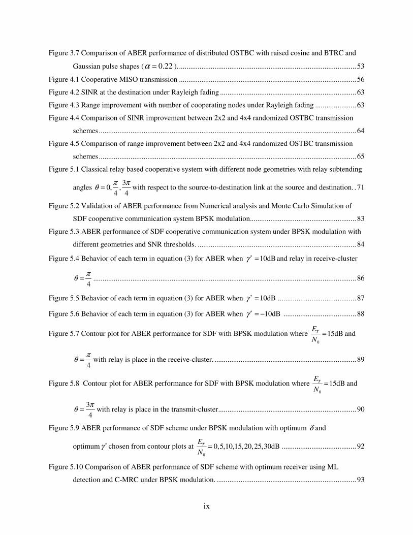
ix

Figure 3.7 Comparison of ABER performance of distributed OSTBC with raised cosine and BTRC and

Gaussian pulse shapes ( 0.22α = )................................................................................................ 53

Figure 4.1 Cooperative MISO transmission ............................................................................................... 56

Figure 4.2 SINR at the destination under Rayleigh fading ......................................................................... 63

Figure 4.3 Range improvement with number of cooperating nodes under Rayleigh fading ...................... 63

Figure 4.4 Comparison of SINR improvement between 2x2 and 4x4 randomized OSTBC transmission

schemes.......................................................................................................................................... 64

Figure 4.5 Comparison of range improvement between 2x2 and 4x4 randomized OSTBC transmission

schemes.......................................................................................................................................... 65

Figure 5.1 Classical relay based cooperative system with different node geometries with relay subtending

angles 3

0, ,4 4π πθ = with respect to the source-to-destination link at the source and destination. .71

Figure 5.2 Validation of ABER performance from Numerical analysis and Monte Carlo Simulation of

SDF cooperative communication system BPSK modulation......................................................... 83

Figure 5.3 ABER performance of SDF cooperative communication system under BPSK modulation with

different geometries and SNR thresholds. ..................................................................................... 84

Figure 5.4 Behavior of each term in equation (3) for ABER when 10dBγ ∗ = and relay in receive-cluster

4πθ = ............................................................................................................................................. 86

Figure 5.5 Behavior of each term in equation (3) for ABER when 10dBγ ∗ = .......................................... 87

Figure 5.6 Behavior of each term in equation (3) for ABER when 10dBγ ∗ = − ....................................... 88

Figure 5.7 Contour plot for ABER performance for SDF with BPSK modulation where 0

15dBTEN

= and

4πθ = with relay is place in the receive-cluster. ............................................................................ 89

Figure 5.8 Contour plot for ABER performance for SDF with BPSK modulation where 0

15dBTEN

= and

34πθ = with relay is place in the transmit-cluster.......................................................................... 90

Figure 5.9 ABER performance of SDF scheme under BPSK modulation with optimum δ and

optimumγ ∗ chosen from contour plots at 0

0,5,10,15,20,25,30dBTEN

= ........................................ 92

Figure 5.10 Comparison of ABER performance of SDF scheme with optimum receiver using ML

detection and C-MRC under BPSK modulation. ........................................................................... 93

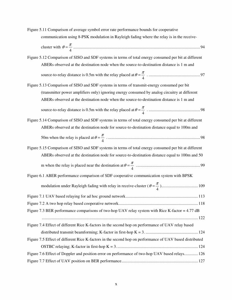
x

Figure 5.11 Comparison of average symbol error rate performance bounds for cooperative

communication using 8-PSK modulation in Rayleigh fading where the relay is in the receive-

cluster with 4πθ = ......................................................................................................................... 94

Figure 5.12 Comparison of SISO and SDF systems in terms of total energy consumed per bit at different

ABERs observed at the destination node when the source-to-destination distance is 1 m and

source-to-relay distance is 0.5m with the relay placed at4πθ = . ................................................. 97

Figure 5.13 Comparison of SISO and SDF systems in terms of transmit-energy consumed per bit

(transmitter power amplifiers only) ignoring energy consumed by analog circuitry at different

ABERs observed at the destination node when the source-to-destination distance is 1 m and

source-to-relay distance is 0.5m with the relay placed at4πθ = . ................................................. 98


ABERs observed at the destination node for source-to-destination distance equal to 100m and

50m when the relay is placed at4πθ = . ........................................................................................ 98


ABERs observed at the destination node for source-to-destination distance equal to 100m and 50

m when the relay is placed near the destination at4πθ = . ............................................................ 99

Figure 6.1 ABER performance comparison of SDF cooperative communication system with BPSK

modulation under Rayleigh fading with relay in receive-cluster (4πθ = )................................... 109

Figure 7.1 UAV based relaying for ad hoc ground network..................................................................... 113

Figure 7.2 A two hop relay based cooperative network............................................................................ 118

Figure 7.3 BER performance comparisons of two-hop UAV relay system with Rice K-factor = 4.77 dB

..................................................................................................................................................... 122

Figure 7.4 Effect of different Rice K-factors in the second hop on performance of UAV relay based

distributed transmit beamforming; K-factor in first-hop K = 3. .................................................. 124

Figure 7.5 Effect of different Rice K-factors in the second hop on performance of UAV based distributed

OSTBC relaying; K-factor in first-hop K = 3. ............................................................................. 124

Figure 7.6 Effect of Doppler and position error on performance of two-hop UAV based relays............. 126

Figure 7.7 Effect of UAV position on BER performance......................................................................... 127

xi

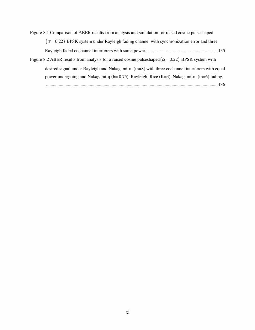
Figure 8.1 Comparison of ABER results from analysis and simulation for raised cosine pulseshaped

( )0.22α = BPSK system under Rayleigh fading channel with synchronization error and three

Rayleigh faded cochannel interferers with same power. ............................................................. 135

Figure 8.2 ABER results from analysis for a raised cosine pulseshaped ( )0.22α = BPSK system with

desired signal under Rayleigh and Nakagami-m (m=8) with three cochannel interferers with equal

power undergoing and Nakagami-q (b= 0.75), Rayleigh, Rice (K=3), Nakagami-m (m=6) fading.

..................................................................................................................................................... 136

xii

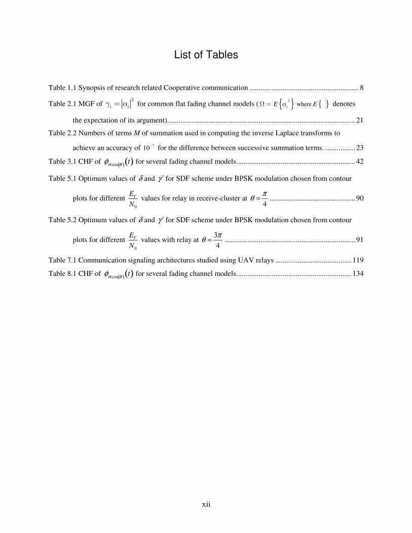
List of Tables

Table 1.1 Synopsis of research related Cooperative communication ........................................................... 8

Table 2.1 MGF of 2

i i for common flat fading channel models ( 2 where

iE E denotes

the expectation of its argument)..................................................................................................... 21

Table 2.2 Numbers of terms M of summation used in computing the inverse Laplace transforms to

achieve an accuracy of 710 for the difference between successive summation terms. ................ 23

Table 3.1 CHF of φα cos θ( ) t( ) for several fading channel models................................................................ 42

Table 5.1 Optimum values of δ and γ ∗ for SDF scheme under BPSK modulation chosen from contour

plots for different 0

TEN

values for relay in receive-cluster at 4πθ = .............................................. 90

Table 5.2 Optimum values of δ and γ ∗ for SDF scheme under BPSK modulation chosen from contour

plots for different 0

TEN

values with relay at 34πθ = ...................................................................... 91

Table 7.1 Communication signaling architectures studied using UAV relays ......................................... 119

Table 8.1 CHF of φα cos θ( ) t( ) for several fading channel models.............................................................. 134

1

Chapter 1

1 Introduction and literature survey

Proliferation of personal wireless enabled devices in the past few years; cell phones, laptops and

PDAs; have made information easily accessible. The growing desire among consumer’s for

pervasive computing has signaled a new wave of interest in ad-hoc [1]-[3] and sensor networks

[4],[5]. These technologies are poised to have a significant impact throughout our society that

could possibly dwarf previous milestones of the information revolution [5]-[8]. Some of the

future applications that could bear the fruits of research in these fields include home networking

and multimedia, environment sensing, telematics for intelligent transportation, industrial

automation, inventory management, rapid network deployment for disaster response, patient

health monitoring and medical care, tactical warfare and social networking. Connectivity is the

key to the success of these applications, which is most likely to consist of heterogeneous devices

with varying computational capability and with a premium on energy consumed. These systems

are likely to compete for scarce spectrum for wireless communication.

Cellular and WLAN are two of the existing mature wireless technologies that follow a hub and

spoke approach where wireless devices only talk to a base-station or access-point with

centralized control over resource allocation. On the other hand, ad-hoc or mesh based networks

achieve end-to-end communication between a source node and a destination node through

multiple point-to-point hops over intermediate nodes that double up as routers or relays.

Research in ad-hoc wireless networks has traditionally focused on modifying link and network

layer negotiation based protocols for resource and topology management for higher throughput

2

and energy efficiency. Recently, measurement results reported from ad-hoc network

implementations have shown that throughput decreases rapidly as the number of hops between

the source and destination becomes greater than two [9]-[11]. This is due to the fact that current

networking models do not properly account for the variations in the physical layer that affect the

link quality. Each hop in a route can experience a different link quality (e.g. outage probability)

that is time varying in nature. On the other hand if the effect of fading is taken into account for

routing in such dynamic ad-hoc networks it would require frequent updates of routing tables with

huge overhead in terms of bandwidth. Therefore a case supporting routes using more reliable

longer and fewer number of hops as opposed to a large number of shorter hops for adhoc

networks was made in [11].

Recently, end-to-end communication that uses cooperation between multiple terminals was

proposed for wireless networks [20]. According to this scheme spatially distributed terminals

form a virtual antenna array through cooperation. These nodes then relay the information from

the source to the destination using parallel hops. Using information theoretic analysis

researchers have so far shown that by fully exploiting the broadcast nature of the wireless

channel and spatial diversity of transmission from cooperating nodes, cooperative

communication can be an effective way for improving capacity.

In the following section we present the concept and background on cooperative communication.

1.1 Cooperative Communication

Advances made in multiple-input-multiple-output (MIMO) signal processing techniques [12],

[13] for communication over point-to-point links using multiple collocated antennas at the

transmitter as well as the receiver have shown tremendous improvements in reliability and

3

throughput. These techniques can be used to improve the weaker link problem mentioned earlier

for ad hoc networks. However due to size, cost and hardware constraints the use of MIMO

techniques in ad-hoc networks may not always be feasible especially in small devices. This has

recently spawned interest in “many-to-many” or “cluster-to-cluster” communication which

involves making single antenna network nodes cooperatively transmit and receive by forming

virtual antenna arrays. This method is broadly named as cooperative communication. However

the idea is to make these virtual arrays to mimic a MIMO system and hence derive better

performance. Figure 1.1 shows a representation of such a cooperative communication scheme.

Source NodeCooperating Tx Node

Cooperating Rx NodeDestination Node

Source NodeCooperating Tx Node

Cooperating Rx NodeDestination Node

Figure 1.1 Representation of cluster-to-cluster communication scheme

Relay nodes which are intermediate nodes present in close vicinity to either the source or

destination form the basis for cooperative communication where they collaborate for

transmission. Next we look at the basic relaying models based on which the cooperative

communication system is studied.

1.1.1 Relaying methods

Two basic relaying methods commonly used for cooperation are discussed below.

4

Decode and forward:

In decode and forward method a cooperating node first decodes signals received from a source

and then relays or retransmits them. The receiver at the destination uses information

retransmitted from multiple relays and the source (when available) to make decisions. It should

be noted that it is possible for a cooperating node to decode symbols in error resulting in error

propagation. Perfect regeneration at the relays may require retransmission of symbols or use of

forward error correction (FEC) depending on the quality of the channel between the source and

the relays. This may not be suitable for a delay limited networks.

Amplify and forward:

In this method each cooperating node receives the signals transmitted by the source node but do

not decode them. These signals in their noisy form are amplified to compensate for the

attenuation suffered between the source-to-relay links and retransmitted. The destination requires

knowledge of the channel state between source-to-relay links to correctly decode the symbols

sent from the source. This requires transmission of pilots over the relays resulting in overhead in

terms of additional bandwidth. Additionally sampling, amplifying, and retransmitting analog

values is a nontrivial task for real-time implementation.

The next section briefly discusses the relaying architectures found in literature.

1.1.2 Relaying architectures

Fig. 1.2 shows various relaying architectures that reduce to commonly used channel models in

the absence of cooperation as explained in [20]. At the heart of cooperative communication is the

classical relay architecture as shown in Fig. 1.2 (a), which is also called the “three body

problem”. In the figure S is the source, R is the relay and D is the destination terminal. The

5

source broadcasts the signal to both the relay and destination. The relay then retransmits the

information to the destination. When the destination is unable to hear the source, the architecture

reduces to the case of cascade multihop communication. When the source and the relay

cooperate to transmit information simultaneously to the destination this reduces to a multiple-

access channel as shown in Fig. 1.2 (b). When the relay and the destination cooperate this

reduces to a broadcast problem as shown in Fig. 1.2 (c). Fig 1.2 (d) shows a simple case of multi-

branch relaying using two parallel branches of relays. When the relays near the source and the

relays near the destination cooperate the case reduces to a simple cluster-to-cluster

communication with interference as shown in Fig. 1.2 (e). This can be viewed as the nodes at the

source cluster broadcasting and the nodes at the receiver in multiple-access mode.

S

R

D

S1

D

S2

S

R1

R2

S1

S2

D1

D2

(a)

(b)

(d) (e)

D1

S

D2(c)

D

Figure 1.2 Relaying architectures: (a) Classical relay; (b) Multiple access channel relaying; (c) Broadcast channel relaying; (d) Multi-branch parallel relaying; (e) Interference channel relaying

6

Next we describe some of the signaling techniques that have been proposed in literature for relay

based cooperative communication.

1.1.3 Signaling techniques for cooperative communication

In this section we give a basic description of some of the most common techniques discussed in

literature for cooperative communication.

Distributed space-time coding:

This type of signaling is similar to space-time block coding (STBC) technique used with multiple

collocated antenna transmitters and receivers. In this scheme nodes cooperate and encode the

signal using STBC such that each node transmits a column of the block code. This idea was first

described in [21]. The advantage of using space-time coding is that it is ideally suited to take

advantage of spatial diversity available in cooperative communication in a bandwidth efficient

manner.

Distributed beamforming:

This is based on the principle of transmit beamforming or transmit-maximal ratio combining

(MRC) when channel state information is available at the transmitter. In environments where

spatial diversity gains are limited, for example air-to-ground communication, transmit

beamforming is known to increase the average SNR at the receiver. Implementation of

cooperative beamforming requires feedback of channel state information (CSI) at each of the

cooperating transmit nodes from the receiver. Performance of this scheme was first reported for

use in sensor network application in [61].

Based on these fundamental relaying methods, architectures and signaling strategies most of the

initial researches on cooperative communication have focused on performance improvements

7

over traditional methods of multi-hop communication in the asymptotic regime. The next section

gives an overview of these works.

1.2 Literature review

Van der Meulen [14] and Cover et al. [15] first reported information theoretic study on the relay

channels under additive white Gaussian channels. The analysis assumes a relay node that has the

ability to simultaneously transmit and receive. Even though this is not directly applicable to a

wireless network where relay transmission poses a half-duplex constraint it is important from a

historical perspective as one of the first works to study relay based communication. Recently,

however there has been a resurgence in theoretical studies in relay based communication that

take the half duplex constraint into account. These are divided into two broad categories. The

first is called the non-compound relay mode where the relays at any time are in one of the two

states, receive or transmit [16]-[19]. In the second case called the compound mode, the relays

transmit using a time division approach where a certain time slot is reserved for transmitting

their own information and the rest of the time slots are used to relay information received from a

partner node [23]-[25], [28], [29].

Table 1.1 shows a synopsis of most of the related literature found on cooperative communication

followed by a summary and brief discussion open issues on the topic. The following are used to

categorize the research papers: a) Information Theoretic b) Coding theory related c)

Performance analysis d) Implementation tradeoffs (bandwidth, energy, complexity) e) System

design issues (synchronization, protocol design) f) Real-time validation g) Year of publication.

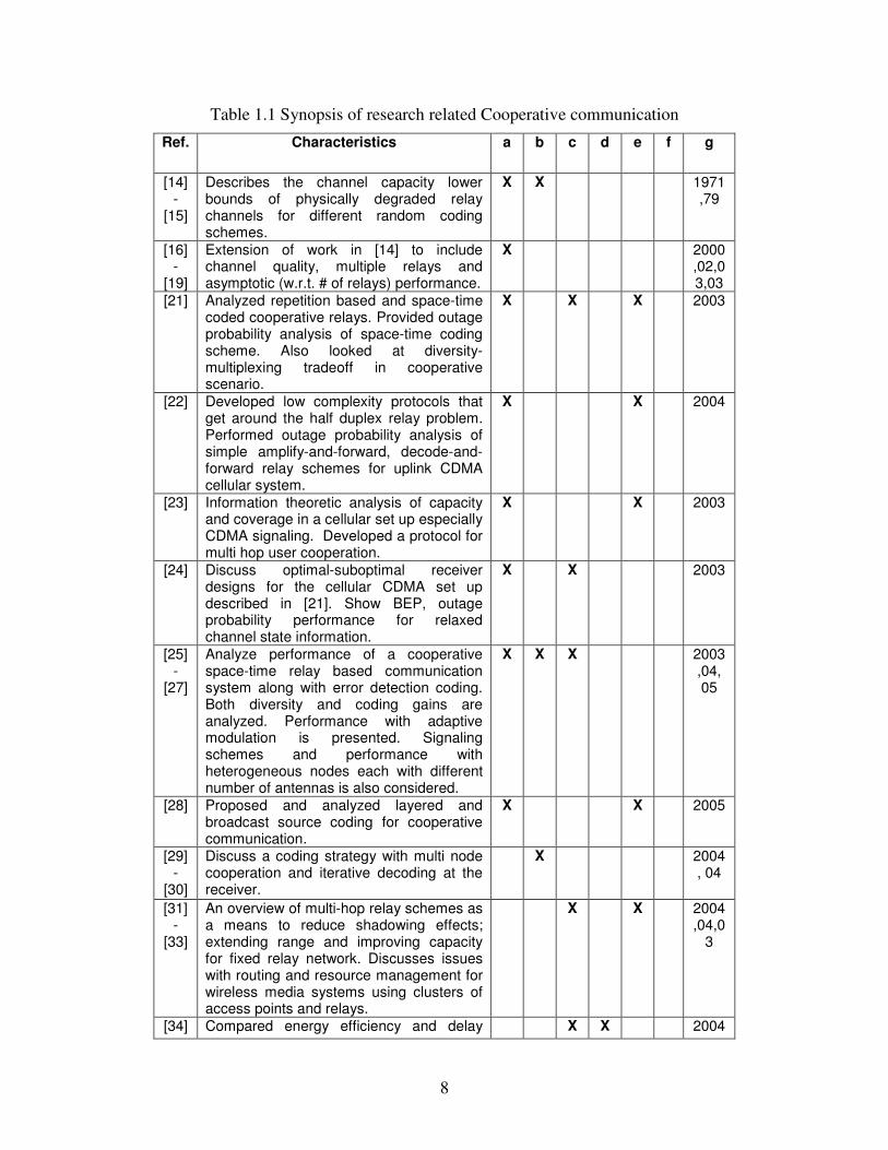
8

Table 1.1 Synopsis of research related Cooperative communication

Ref. Characteristics a b c d e f g

[14]-

[15]

Describes the channel capacity lower bounds of physically degraded relay channels for different random coding schemes.

X X 1971,79

[16]-

[19]

Extension of work in [14] to include channel quality, multiple relays and asymptotic (w.r.t. # of relays) performance.

X 2000,02,03,03

[21] Analyzed repetition based and space-time coded cooperative relays. Provided outage probability analysis of space-time coding scheme. Also looked at diversity-multiplexing tradeoff in cooperative scenario.

X X X 2003

[22] Developed low complexity protocols that get around the half duplex relay problem. Performed outage probability analysis of simple amplify-and-forward, decode-and-forward relay schemes for uplink CDMA cellular system.

X X 2004

[23] Information theoretic analysis of capacity and coverage in a cellular set up especially CDMA signaling. Developed a protocol for multi hop user cooperation.

X X 2003

[24] Discuss optimal-suboptimal receiver designs for the cellular CDMA set up described in [21]. Show BEP, outage probability performance for relaxed channel state information.

X X 2003

[25]-

[27]

Analyze performance of a cooperative space-time relay based communication system along with error detection coding. Both diversity and coding gains are analyzed. Performance with adaptive modulation is presented. Signaling schemes and performance with heterogeneous nodes each with different number of antennas is also considered.

X X X 2003,04, 05

[28] Proposed and analyzed layered and broadcast source coding for cooperative communication.

X X 2005

[29]-

[30]

Discuss a coding strategy with multi node cooperation and iterative decoding at the receiver.

X 2004, 04

[31]-

[33]

An overview of multi-hop relay schemes as a means to reduce shadowing effects; extending range and improving capacity for fixed relay network. Discusses issues with routing and resource management for wireless media systems using clusters of access points and relays.

X X 2004,04,0

3

[34] Compared energy efficiency and delay X X 2004

9

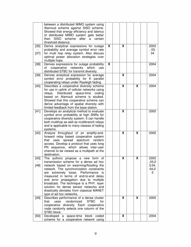
between a distributed MIMO system using Alamouti scheme against SISO scheme. Showed that energy efficiency and latency of distributed MIMO system gets better than SISO scheme after a certain threshold distance.

[35]-

[37]

Derive analytical expressions for outage probability and average symbol error rate for multi hop relay system. Also discuss optimal power allocation strategies over multiple hops.

X X 2003, 03, 04

[38] Derives expressions for outage probability of cooperative networks which use distributed STBC for transmit diversity.

X 2004

[39] Derives analytical expression for average symbol error probability for K parallel cooperating relays under Rayleigh fading.

X 2004

[40] Describes a cooperative diversity scheme for use in uplink of cellular networks using relays. Distributed space-time coding based on Alamouti scheme is studied. Showed that this cooperative scheme can derive advantage of spatial diversity with limited feedback from the base station.

X X 2004

[41] Develops an analytical method to evaluate symbol error probability at high SNRs for cooperative diversity system. It can handle both multihop as well as multibranch relays and is applicable to many classes of fading systems.

X 2005

[42] Analyze throughput of an amplify-and-forward relay based cooperative system that uses spread spectrum random access. Develop a protocol that uses long PN sequence, which allows inter-user channel to be viewed as a multipath at the destination.

X X 2005

[43]-

[48]

The authors propose a new form of transmission scheme for a dense ad hoc network based on swarming/flooding the network. The synchronization constraints are extremely loose. Performance is measured in terms of end-to-end delay and error propagation due to multiple broadcast. The technique is a PHY. layer solution for dense sensor networks and drastically deviates from classical MANET type of ad hoc networks.

X X 2003,03,03,04, 04,0

5

[49] Describes performance of a dense cluster that uses randomized STBC for cooperative diversity. Each cooperative node randomly selects one column of the STBC block.

X X 2005

[50] Developed a space-time block coded scheme for a cooperative network using

X 2004

10

more than two hops. Performance in terms of frame error rate was evaluated using simulation for slow and fast fading cases.

[51] Develop a differential modulation scheme for two user cooperative diversity systems. The scheme does not require CSI. Also develop an incremental relaying protocol, which is shown to perform better than standard decode-and-forward relay scheme.

X X 2004

[52]-

[58]

Developed new techniques for cooperative transmission which include new space-time coding technique [51], active phase rotation at relays that take perform active scattering [52], transmit power allocation scheme over cooperating relays [53], distributed spatial multiplexing [54], capacity evaluation [55], scheduling [56] and minimizing error performance under noisy CSI [57].

X X X X X 2003,04,04,04,04,04,05

[59] Analyze outage probability of a cooperative network with a certain node distribution. This is compared to the case when there is no cooperation.

X X 2005

[60] Analyze BER performance of a DSTC scheme based on source/relay link quality. Develop and analyze optimum and sub-optimum receivers and present their performance. Discuss tradeoffs between rate loss and reliability improvement for a BPSK constellation.

X X 2005

[61] Describes the BER performance of a DSTC cellular system using two mobile stations. Presents analysis for computing average path loss under different spatial distributions. This is plugged into BER computation to show that in most scenarios compared to a collocated antenna system with same number of antennas the loss is less than 2 dB.

X X 2004

[62]-

[64]

Present performance analysis of distributed beamforming in a sensor network by analyzing the improvement in SNR [61], show a method to adaptively co-phase signals using a feedback loop [62] and show improvement in average directivity of the beam in a dense sensor network as the number of nodes increase [63].

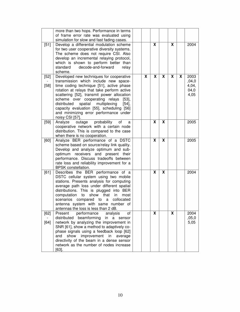
X X 2004,05,05,05

11

[65] It is shown that there exists a collaborative code, which can satisfy a given performance requirement for certain types of relay channels. Outage probability analysis is presented for a DSTC case where relays listen and transmit asynchronously. It is shown that if the intra-cluster path loss has a at least 10dB advantage over source destination link then there is negligible penalty for collaboration when compared with traditional space-time coding.

X X 2005

[66] Investigates ergodic and outage probability for amplify-and-forward cooperative relays with different transmission protocols.

X 2004

[67] Examine and compare performance in terms of information theoretic capacity and diversity achieved by three suggested protocols for a single source-relay-destination configuration. Both decode-and-forward and amplify-and-forward relay cases are studied for each protocol. It is shown that depending on the protocol used and based on the condition of operation under ideal conditions the system can viewed as a distributed MIMO (mainly multiplexing gain), MISO or SIMO (diversity gain) system.

X X 2004

[68] Propose and analyze capacity scaling laws for distributed dense wireless networks under non-ideal conditions of imperfect synchronization and CSI.

X 2005

Some important observations and open issues that emerge from this survey are summarized

below.

Most of the research on the topic focuses on information theoretic analysis for achievable

capacity and developing mathematical framework for capacity scaling laws under increasing

network node densities. Most of these results apply to communication under high SNR regime.

12

The analyses presented in most of the works assume ideal conditions of operation, i.e.,

transmission and reception under perfect synchronization and perfect channel state information

(CSI). The channels considered are either frequency non-selective Rayleigh fading or AWGN.

The wireless links that constitute a cooperative communication set up are typically assumed to be

identical. In a distributed set up this need not be true as some of the links may experience line-of-

sight (LoS) channels and others non-line-of-sight (NLoS).

As the node density increases the average transmit power of a cluster of cooperating nodes as a

whole also increases suggesting a potential application in range improvement. The distributed

nature of transmission also means that in networks where nodes are limited in energy supply

from a battery the burden can now be distributed over multiple nodes through cooperation. This

holds the possibility of improvements in network lifetime. Hence benefits other than capacity

improvement should not be overlooked.

In the real world acquisition and tracking of signals for synchronization and cooperation among

nodes can be complex requiring a lot of resources. Enabling technologies such as high precision

GPS assisted atomic clocks [68] may help alleviate some of the problems in future. There may

be a need for a cross-layer approach to design protocols that combine network timing that is

mostly handled by MAC layer and synchronization of the nodes at the physical layer using

enabling technologies like a GPS.

1.3 Key contributions

Based on the literature review presented above, most of the researches have relied on

information theoretic analysis under constraints of orthogonal transmission or operation under

ideal conditions. While the relaxed constraints make the prospect of relaying appear more

13

feasible, there is considerable amount of research that needs to be done before complete end-to-

end solutions are developed that not only enjoy the benefits of cooperative communication but

also become practically realizable. In this dissertation we investigate the limits and tradeoffs of

cooperative communication under timing error, imperfect relaying and non identical cooperating

wireless links. In addition to capacity and bit error rate performance we also investigate the

potential for range and energy efficiency improvements. The main contributions are summarized

as follows:

• We provide a framework for efficient analysis of outage and ergodic capacities of

distributed orthogonal space-time coding system where the cooperating links can be

operating under different fading channels or with different SNRs.

• Cooperative transmission using distributed orthogonal space-time block codes (OSTBC)

for exploiting cooperative diversity was first suggested in [21]. However it was assumed

that the distributed nodes are perfectly synchronized in time. In practical systems time

synchronization errors are known to degrade the performance. In our work we

characterize the effect of timing synchronization error on the bit error rate performance of

distributed OSTBC system. We show that under certain channel conditions distributed

OSTBC with timing error can perform better than a perfectly synchronized single-input-

single-output (SISO) system.

• A new technique called randomized space-time block coding for cooperative

communication was proposed in [49] for better diversity reception in a cooperative

network. Since diversity reception does not require stringent co-phasing of signals as in

cooperative beamforming we investigate the range improvement achieved by using the

above scheme under timing errors as the number of cooperating nodes increase.

14

• Several adaptive versions of decode and forward cooperative diversity protocols have

been proposed and studied in the past. However, in most researches it is assumed that the

relays perfectly decode and regenerate the bits received from the source. However such

an assumption can lead to error propagation resulting in wrongful combining at the

destination. Hence in this research we derive an end-to-end average bit error rate for a

simple source-relay-destination cooperative communication system by accounting for

imperfect relaying. In addition we establish a simple framework that allows us to explore

the effect of placement of the relay and different fading conditions on the performance of

a decode-and-forward system. We analyze the performance of two simple selective

decode-and-forward (SDF) schemes, the first based on SNR threshold and the second

based on a log-likelihood ratio (LLR) threshold based relying that lend themselves to

easier implementation than optimal decode-and-forward systems [24].

• As mentioned earlier in section 1.2 higher energy efficiency may be one of the potential

benefits of cooperative communication when compared to point-to-point communication

especially in networks where nodes are energy limited. We apply the knowledge of end-

to-end ABER performance of a simple decode-and-forward set up described above to

investigate energy efficiency gains. It is shown that it is possible to have energy efficient

transmission using decode-and-forward scheme under certain different propagation

conditions and geometry of the nodes.

1.4 Organization of thesis

The following gives a roadmap to reading this thesis. In Chapter 2 we discuss a numerical

technique to evaluate the outage and ergodic capacity of a distributed orthogonal space-time

15

coding system under generalized fading. This is specifically suited for capacity analysis of non-

identically distributed channels that cooperative-communication systems are more likely operate

under. In Chapter 3 we present a frequency domain analysis of the effect of time

synchronization errors on the ABER of a bandlimited multiple-input-single-output (MISO)

distributed OSTBC system. In Chapter 4 we discuss the relationship between range improvement

and the number of nodes participating in cooperative communication using randomized space-

time coding under timing errors. In Chapter 5 we present the end-to-end ABER analysis for two

selective decode-and-forward protocols and establish a framework to analyze the effect of

location of the relay and fading on the performance. Based on the ABER results we further

investigate the energy efficiency of the system and compare it with a SISO system. In chapter 6

we present the analysis for a SDF system where the relay uses a log-likelihood ratio based

criterion to selectively forward information. In Chapter 7 we discuss a potential application of

cooperative communication using air-to-ground communication over single antenna mounted

UAVs to improve performance of ground based adhoc networks. In Chapter 8 we apply the

method developed in chapter 3 for analysis of the effect of timing errors and asynchronous

cochannel interference on a bandlimited narrowband system under different fading channels. We

draw our conclusions in Chapter 9 and with a brief discussion on future work.

16

Chapter 2

2 Outage and ergodic capacities of distributed OSTBC cooperative networks

In point-to-point communication systems that use multiple antennas at the transmitter and

receiver, maximum spatial diversity benefits are obtained when the antennas are spaced

sufficiently far apart such that the fading statistics on different diversity paths are uncorrelated.

This constraint precludes the use of antenna arrays in many scenarios such as mobile handsets

and low profile sensor nodes. Recent work in cooperative communications [21] has suggested

collaboration among multiple single antenna users to overcome the above problem. As explained

in Chapter 1 communication nodes form “partnerships” and pool their antenna resources to form

a virtual antenna array to exploit cooperative diversity advantages without the actual use of

antenna arrays at each node. In this chapter we explore the performance of a cooperative MIMO

system that uses orthogonal space-time block coding.

Among various diversity/multiplexing MIMO solutions such as BLAST [71], orthogonal space-

time block coding (OSTBC) [72] and space-time trellis coding [73], distributed OSTBC is an

attractive solution for energy-constrained sensor networks because it does not require additional

bandwidth and possesses low encoding-decoding complexity. Outage and ergodic capacities are

important measures of performance of a communication system under fading channels. In [20],

[21], [38], outage probability of distributed OSTBC systems were investigated. However the

analyses assume similar distributions for cooperating wireless links. In practice however when

nodes are spatially distributed it is more likely that the cooperating links experience different

types of channels. For example one link may experience a line-of-sight (LoS) channel and

17

another non-line-of-sight (NLoS). The contribution of the work presented in this chapter is the

development of a general yet simple numerical approach for evaluating both the ergodic capacity

and the outage capacity of cooperative networks that use distributed OSTBC and distributed

diversity receiver in generalized fading channels, for which, the fading statistics across the

virtual antenna array elements need not be identically distributed, nor even distributed according

to the same family of distributions. Even for the special case of Nakagami-m channel considered

in [38] our result generalizes their results by removing the restriction of positive integer fading

severity index.

Our moment generating function (MGF) based approach is motivated by the fact that finding the

probability density function (PDF) of signal-to-noise-ratios (SNRs) at the output of OSTBC

decoder in closed form is often very restrictive to some special cases, while its MGF can be

obtained in a compact form (as a product of individual path MGFs) for a wide range of fading

distributions including Rayleigh, Rice, Nakagami-m, Nakagami-Hoyt and Weibull distributions.

This chapter relies on an efficient fixed Talbot algorithm for numerically inverting the MGF to

obtain its cumulative distribution function (CDF) [74] and its applicability to the ergodic and

outage capacity calculations of distributed OSTBC systems.

2.1 Generic expressions for the ergodic and outage capacities

Fig. 2.1 illustrates a general cooperative sensor network architecture that employs OSTBC and

maximal ratio combining (MRC) or selection diversity combining (SDC) in the receive cluster

for data transmission. The space-time encoded codewords from the cluster head are passed

to TN spatially distributed transmitters and broadcasted to RN spatially distributed nodes in the

receive cluster. The received signals are then passed to the space-time block decoder at the

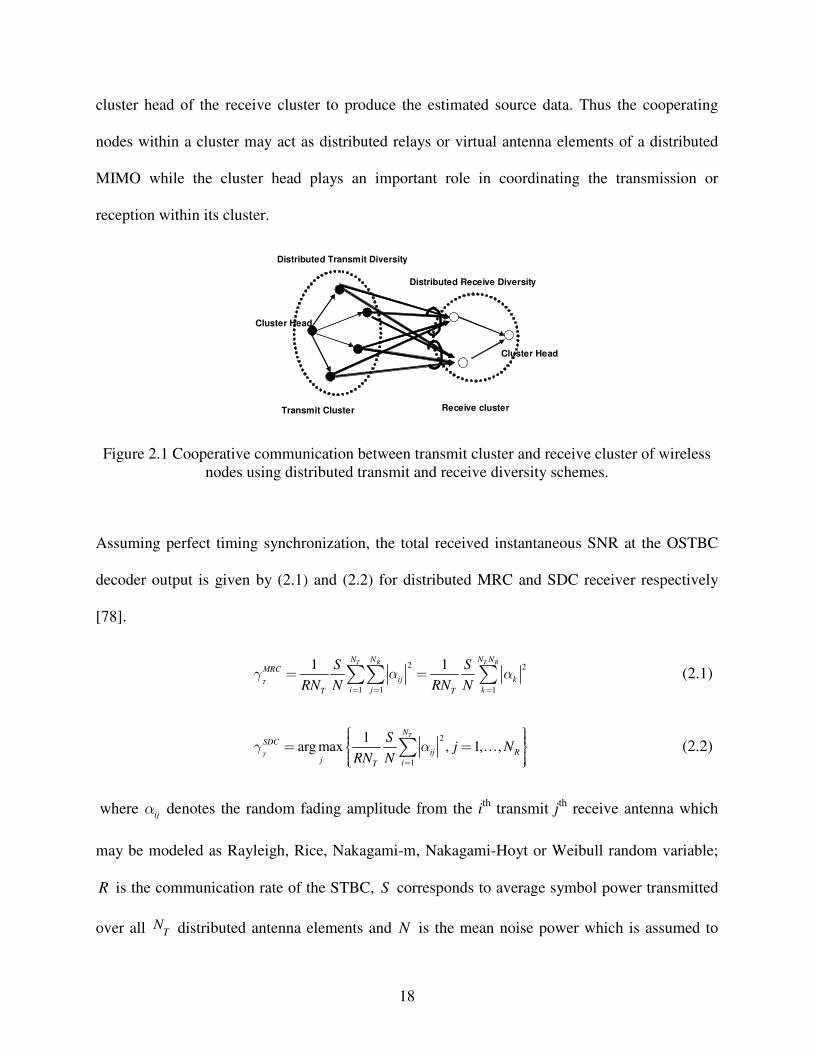
18

cluster head of the receive cluster to produce the estimated source data. Thus the cooperating

nodes within a cluster may act as distributed relays or virtual antenna elements of a distributed

MIMO while the cluster head plays an important role in coordinating the transmission or

reception within its cluster.

Transmit Cluster Receive cluster

Distributed Receive Diversity

Cluster Head

Cluster Head

Distributed Transmit Diversity

Figure 2.1 Cooperative communication between transmit cluster and receive cluster of wireless nodes using distributed transmit and receive diversity schemes.

Assuming perfect timing synchronization, the total received instantaneous SNR at the OSTBC

decoder output is given by (2.1) and (2.2) for distributed MRC and SDC receiver respectively

[78].

2 2

1 1 1

1 1T R T R

T

N N N NMRC

ij ki j kT T

S SRN N RN N

(2.1)

2

1

1arg max , 1, ,

T

T

NSDC

ij Rj iT

Sj N

RN N

(2.2)

where ij denotes the random fading amplitude from the ith transmit jth receive antenna which

may be modeled as Rayleigh, Rice, Nakagami-m, Nakagami-Hoyt or Weibull random variable;

R is the communication rate of the STBC, S corresponds to average symbol power transmitted

over all TN distributed antenna elements and N is the mean noise power which is assumed to

19

be identical for all RN distributed receive antenna elements. Since the cooperating nodes in the

transmitter and receiver clusters are spatially distributed, the transmitted codewords may take

completely different propagation paths before arriving at the OSTBC decoder. Therefore, in our

analysis we shall consider capacity evaluation of distributed OSTBC with dissimilar channel

statistics including the mixed-fading scenario.

The use of OSTBC is known to reduce the MIMO channel into a single-input-single-output

(SISO) channel with modified channel statistics [75], [76] which allows us to write the

instantaneous normalized channel capacity (in bits/second/Hertz) over such MIMO channels as

2log 1 TC R (2.3)

Thus the outage capacity (probability that a specified transmission rate cannot be supported

by the channel) can be calculated as

Tout C TP F F (2.4)

where XF denotes the CDF of random variable , , TX X C and T can be obtained

from (2.3) as 2 1RT

. The ergodic capacity, on the other hand, may be calculated by

taking the statistical average of (2.3) over all channel realizations ij , viz.

2

0

0

log 1

1

ln 2 1

T

T

T T T

TT

T

C R p d

FRd

(2.5)

where T

p denotes the PDF of random variable T . The second line of (2.5) is obtained from

the first line via integration by parts. From (2.4) and (2.5), it is evident that only the knowledge

20

of the CDF of T is further required in the calculation of both the outage capacity and the

ergodic capacity. Notice however that the evaluation of the PDF of MRCT depicted in (2.1)

involves the computational complexity of T RN N -fold nested convolution integral over the PDFs

of 2k . Similarly, the calculation of the PDF of SDC

T depicted in (2.2) involves TN -fold

convolution over the PDFs of 2i . To circumvent this difficulty, we adopt an MGF-based

approach for computing the CDF of T from its MGF which is readily expressed in a simple

form for a wide range of distributions and channel statistics. Specifically, the CDF of MRCT and

SDCT can be calculated as

1

1

1 1T R

T i

N NMRC

i T

SF x LT s

s N RN

! (2.6)

1

1 1

1 1R T

T ij

N NSDC

j i T

SF x LT s

s N RN

! ! (2.7)

where 2i i denotes the normalized instantaneous received SNR of the ith diversity path,

i denotes the MGF of i and " #1LT denotes the inverse Laplace transform of its argument.

Closed form expressions for the MGF of i are summarized in Table 2.1 for several stochastic

channel models commonly used for modeling wireless channels. Two efficient numerical

inversion techniques for computing the CDF of T given the MGF of T are discussed in the

following section.

21

Table 2.1 MGF of 2i i for common flat fading channel models ( 2

where i

E E

denotes the expectation of its argument).

Weibull [14]

Nakagami-q

Nakagami-m

Rice

Rayleigh

MGFFading Parameter

Channel

Weibull [14]

Nakagami-q

Nakagami-m

Rice

Rayleigh

MGFFading Parameter

Channel i

s

11 is

1exp

1 1i i i

i i i i

K K sK s K s

1 im

i is m

2 21 1 2 1i i is s q

1 1

,12 2 1,

12 11

1,1 , ,1

ii

i i i

i

cc

c c cii c i i

i ii i

c sc s G cc

c c

$

0 iK%

0.5 im%

0 1iq% %

0 ic%

,, is the Meijer's G functionm n

p qG

is a positive scale parameteri

2.2 Efficient computation of the Bromwich integral

If integrand Xf t is piecewise continuous, then using the time-integration property of Laplace

transform, we obtain

0 0 0

1xsx sx

X Xe f t dt dx e f x dxs

(2.8)

Therefore the CDF of random variable X , XF x can be computed as the inverse Laplace

transformation of X s s (Bromwich integral). In [76], Abate et. al. suggested evaluating the

Bromwich integral by means of trapezoidal rule approximation and accelerated its convergence

using the Euler summation technique. This leads to

2

,0 0

1 22

2

bAM B cM

X X A B Mc b b

M e A ibF x R R

c x x

& (2.9)

22

where 0 2, 1 for any 1b b ' , & denotes the real part of the complex argument and AR

and ,B MR correspond to the discretization error and series truncation error terms respectively.

The constants A, B and M may be selected to achieve a desired accuracy. This technique has

been used for computing the outage probability and average symbol error rate of diversity

systems over generalized fading channels in [77] and [78] respectively.

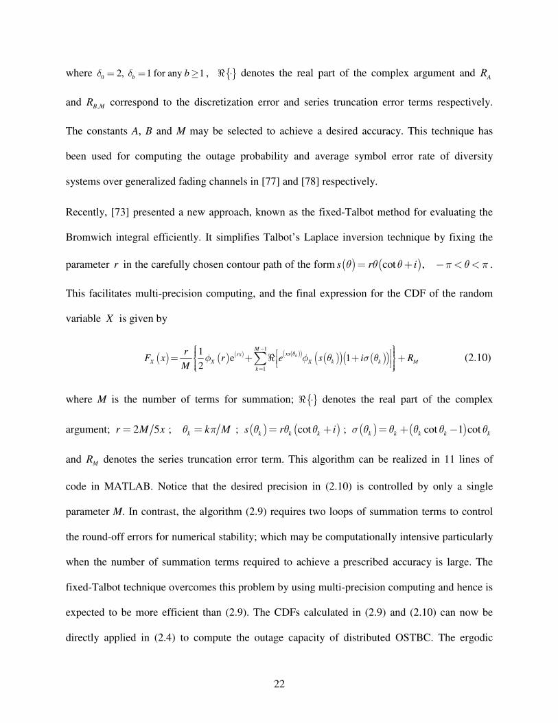
Recently, [73] presented a new approach, known as the fixed-Talbot method for evaluating the

Bromwich integral efficiently. It simplifies Talbot’s Laplace inversion technique by fixing the

parameter r in the carefully chosen contour path of the form cot , s r i ( ( .

This facilitates multi-precision computing, and the final expression for the CDF of the random

variable X is given by

1

1

1e 1

2k

Mxsrx

X X X k k Mk

rF x r e s i R

M

& (2.10)

where M is the number of terms for summation; & denotes the real part of the complex

argument; 2 5r M x ; k k M ; cotk k ks r i ; cot 1 cotk k k k k

and MR denotes the series truncation error term. This algorithm can be realized in 11 lines of

code in MATLAB. Notice that the desired precision in (2.10) is controlled by only a single

parameter M. In contrast, the algorithm (2.9) requires two loops of summation terms to control

the round-off errors for numerical stability; which may be computationally intensive particularly

when the number of summation terms required to achieve a prescribed accuracy is large. The

fixed-Talbot technique overcomes this problem by using multi-precision computing and hence is

expected to be more efficient than (2.9). The CDFs calculated in (2.9) and (2.10) can now be

directly applied in (2.4) to compute the outage capacity of distributed OSTBC. The ergodic

23

capacity of distributed OSTBC can be calculated by substituting (2.9) or (2.10) into (2.5) and

numerically evaluating the resulting expression by a Gauss-Chebyshev integration technique.

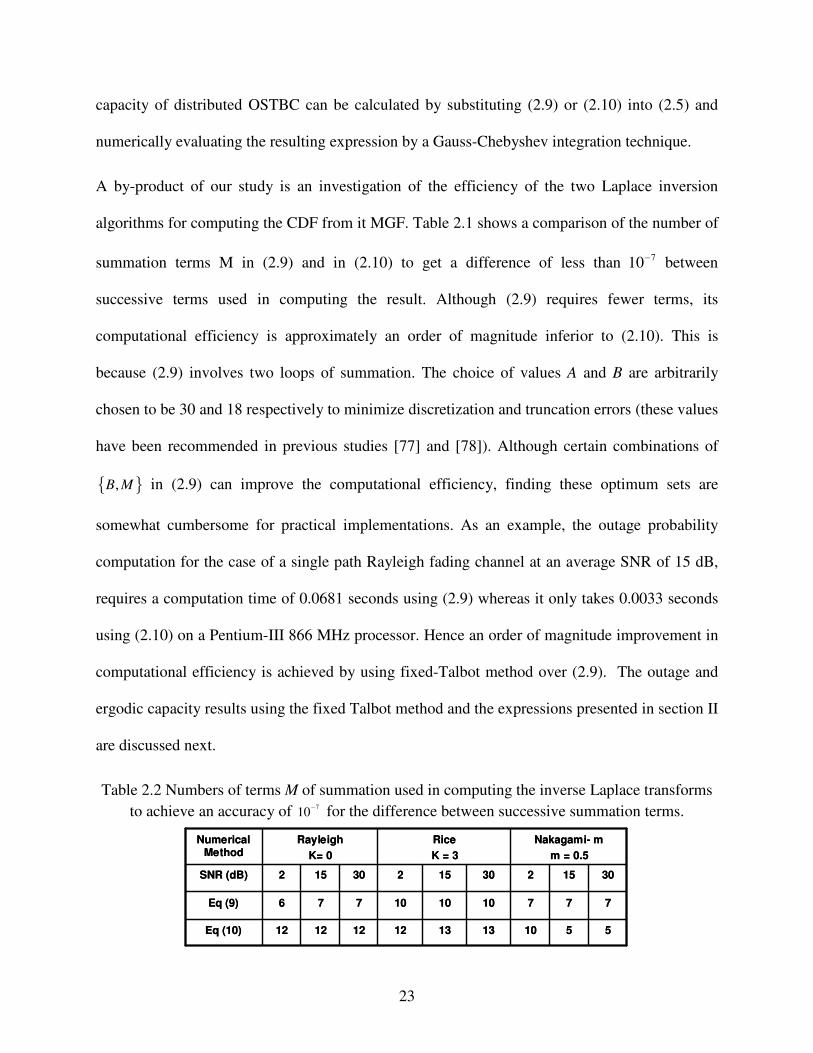
A by-product of our study is an investigation of the efficiency of the two Laplace inversion

algorithms for computing the CDF from it MGF. Table 2.1 shows a comparison of the number of

summation terms M in (2.9) and in (2.10) to get a difference of less than 710 between

successive terms used in computing the result. Although (2.9) requires fewer terms, its

computational efficiency is approximately an order of magnitude inferior to (2.10). This is

because (2.9) involves two loops of summation. The choice of values A and B are arbitrarily

chosen to be 30 and 18 respectively to minimize discretization and truncation errors (these values

have been recommended in previous studies [77] and [78]). Although certain combinations of

,B M in (2.9) can improve the computational efficiency, finding these optimum sets are

somewhat cumbersome for practical implementations. As an example, the outage probability

computation for the case of a single path Rayleigh fading channel at an average SNR of 15 dB,

requires a computation time of 0.0681 seconds using (2.9) whereas it only takes 0.0033 seconds

using (2.10) on a Pentium-III 866 MHz processor. Hence an order of magnitude improvement in

computational efficiency is achieved by using fixed-Talbot method over (2.9). The outage and

ergodic capacity results using the fixed Talbot method and the expressions presented in section II

are discussed next.

Table 2.2 Numbers of terms M of summation used in computing the inverse Laplace transforms to achieve an accuracy of 710 for the difference between successive summation terms.

301523015230152 SNR (dB)

Nakagami- mm = 0.5

RiceK = 3

RayleighK= 0

Numerical Method

13

10

12

10

12

7

12

7

12

6

Eq (10)

Eq (9)

5

7

51013

7710

301523015230152 SNR (dB)

Nakagami- mm = 0.5

RiceK = 3

RayleighK= 0

Numerical Method

13

10

12

10

12

7

12

7

12

6

Eq (10)

Eq (9)

5

7

51013

7710

24

2.3 Results

Fig. 2.2 and 2.3 show the outage probability of a distributed OSTBC cooperative network with

2TN and 2RN for distributed MRC and SDC in the receive cluster respectively. The plots

have been generated for both Rayleigh 0K and Rice 3K , flat fading channel models. We

consider two scenarios where, the average channel gain of each link in the distributed OSTBC

MIMO case is either balanced or unbalanced. In the unbalanced case the distribution of average

channel gain for the four links in the 2x2 system is chosen to be 1.25, 0.25, 0.25 and 0.25 times

the total average channel SNR and in the balanced case each link is 0.5 times the total average

channel SNR. The total average channel SNR given by 21 1

1 R TN N

iji jT

SE

N N

, is fixed at 15 dB.

Plots for balanced 1x2 single-input-multiple-output (SIMO) cooperative network have also been

generated as a reference where, the average channel SNR (and hence the total transmitted power)

is kept the same as in the MIMO case. The plots obtained by analysis match perfectly with

Monte Carlo simulation results validating the accuracy of our mathematical approach and coding.

It can be seen that when the links are balanced, the performance is slightly better than that of

unbalanced case. For an outage probability of 1 0 4 the difference in their outage capacities for

Rice and Rayleigh cases are 0.36 bits/Hz/s and 0.25 bits/Hz/s respectively. This suggests that

links with line-of-sight component get affected more by power imbalances than the non-line-of-

sight case. Comparing 2.2 and 2.3, the performance of distributed MRC is better than distributed

SDC as expected. Also for the same average received SNR at the output of the receive cluster,

for both SIMO as well as MIMO case considered here, the MIMO network outperforms the

SIMO network. Hence cooperation at the transmit cluster using OSTBC improves performance

without increasing the bandwidth requirement. Fig. 2.4 shows the results for normalized ergodic

25

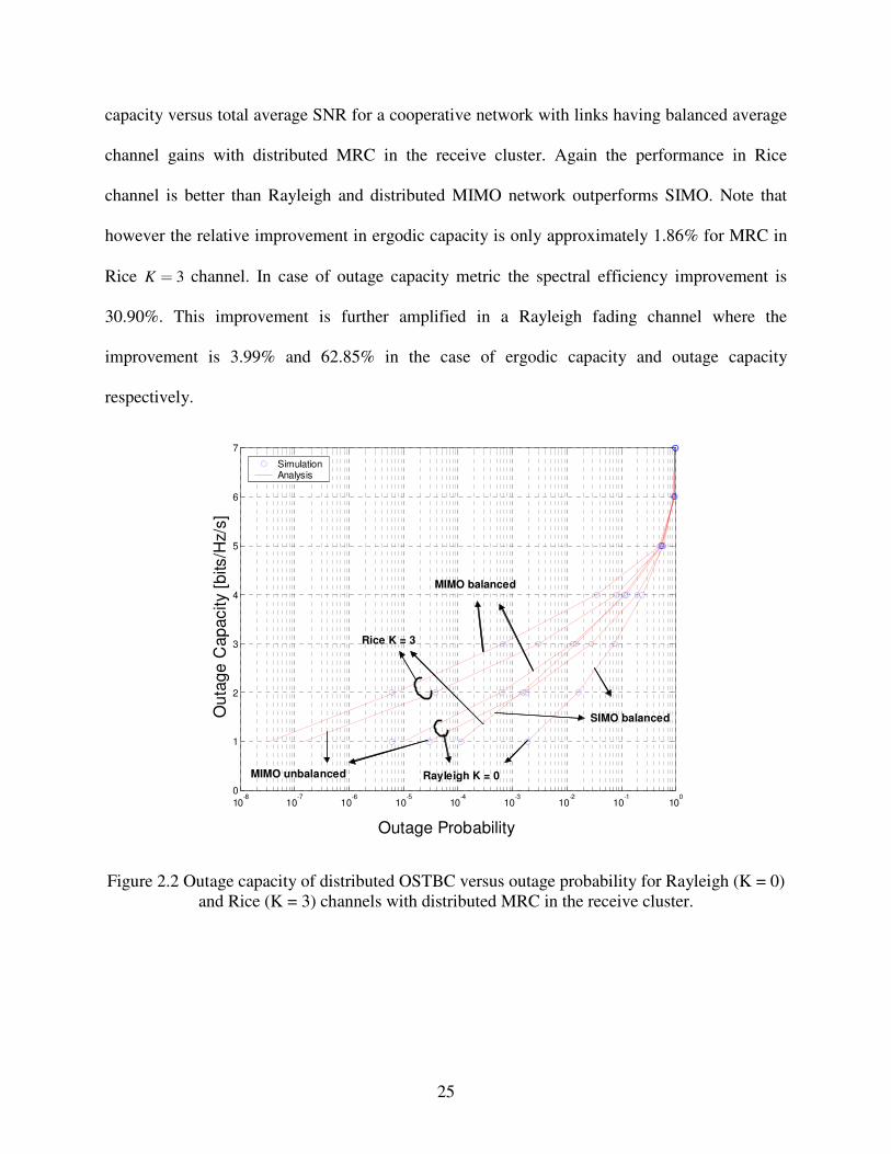
capacity versus total average SNR for a cooperative network with links having balanced average

channel gains with distributed MRC in the receive cluster. Again the performance in Rice

channel is better than Rayleigh and distributed MIMO network outperforms SIMO. Note that

however the relative improvement in ergodic capacity is only approximately 1.86% for MRC in

Rice 3K channel. In case of outage capacity metric the spectral efficiency improvement is

30.90%. This improvement is further amplified in a Rayleigh fading channel where the

improvement is 3.99% and 62.85% in the case of ergodic capacity and outage capacity

respectively.

10-8

10-7

10-6

10-5

10-4

10-3

10-2

10-1

100

0

1

2

3

4

5

6

7

SimulationAnalysis

Out

age

Cap

acity

[bits

/Hz/

s]

Outage Probability

Rayleigh K = 0

Rice K = 3

MIMO unbalanced

MIMO balanced

SIMO balanced

Figure 2.2 Outage capacity of distributed OSTBC versus outage probability for Rayleigh (K = 0) and Rice (K = 3) channels with distributed MRC in the receive cluster.

26

10-7

10-6

10-5

10-4

10-3

10-2

10-1

100

0

1

2

3

4

5

6

7

SimulationAnalysis

Out

age

Cap

acity

[bits

/Hz/

s]

Outage Probability

Rayleigh K = 0

Rice K = 3

MIMO unbalanced

MIMO balanced

SIMO balanced

Figure 2.3 Outage capacity of distributed OSTBC versus outage probability for Rayleigh (K = 0) and Rice (K = 3) channels with distributed SDC in the receive cluster.

0 5 10 150

0.1

0.2

0.3

0.4

0.5

0.6

Rayleigh 1x2 Rx diversityRice 1x2 Rx diversityRayleigh 2x2 OSTBCRice 2x2 OSTBCAWGN 2x2 OSTBC

Log

10(N

orm

aliz

ed E

rgo

dic

Cap

acity

[bits

/Hz/

s])

21 1

1 R TN N

iji jT

SE

N N

dBAverage Channel SNR

Figure 2.4 Normalized ergodic capacity of distributed OSTBC versus average total received channel gain for Rayleigh (K = 0) and Rice (K= 3) channels with distributed MRC in the receive

cluster.

27

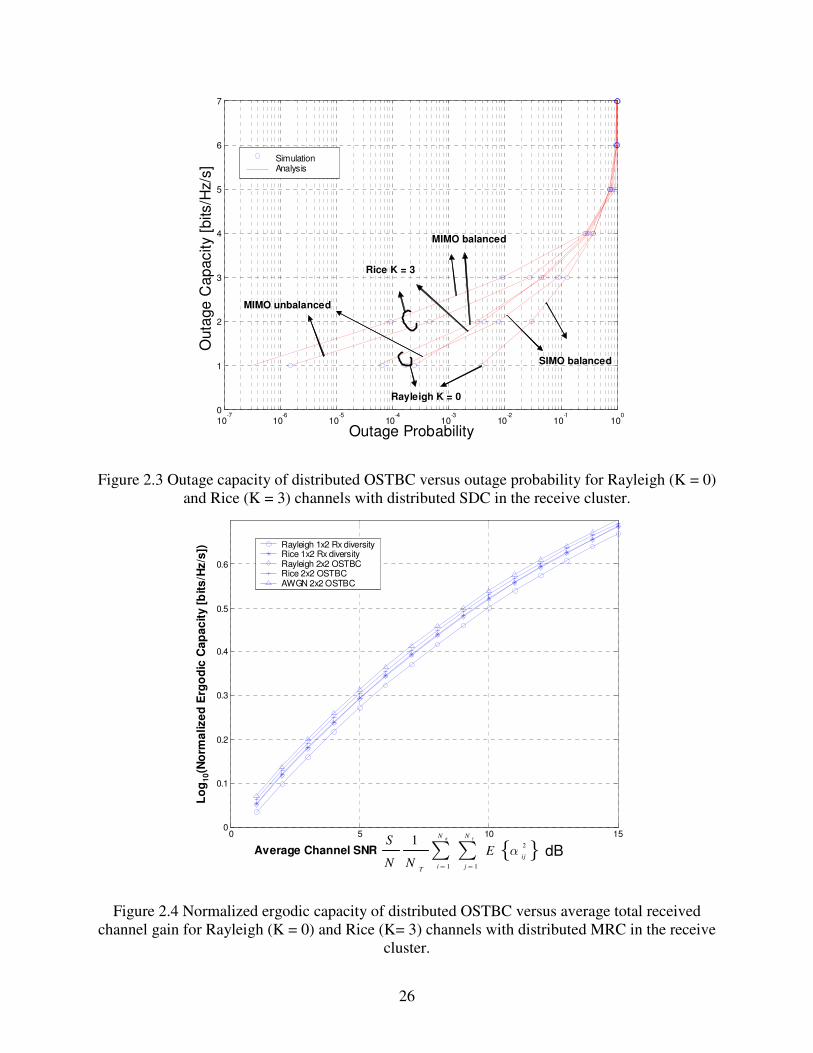
Next we analyze the effect of having different families of fading distributions on different Tx-Rx

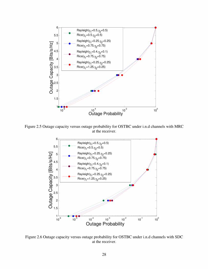
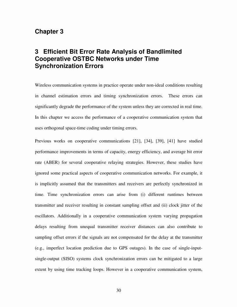
links on the outage capacity of OSTBC. Fig. 2.5 and Fig. 2.6 show the performance of a 2x2

OSTBC system with two links having Rayleigh distribution and the other two having Rice (K=3)

distribution with MRC at the receiver. Both balanced and unbalanced MIMO cases are

considered.

In both cases, MRC as well as SDC, the outage capacity for a certain outage probability is

highest when the links are balanced, i.e.; when all the links have the same average channel SNRs

,0.5

i jγ = times the total average channel SNR. The next best performance is found when the

average SNRs are balanced over the same family of fading statistics. It is interesting to note the

difference in performance for the worst cases in MRC and SDC. In the case of MRC, the worst

case performance is observed when the Rice distributed channels have a high imbalance in

average channel SNRs; whereas in the case of SDC the above distribution has better outage

capacity than when the Rice channels have equal average channel SNRs. This can be attributed

to the fact that in SDC the diversity combiner selects the branch with highest received SNR

which in the case of unbalanced case has a better average received SNR (0.75 Total ) than the

balanced case (0.5 Total ).

28

10-6

10-4

10-2

100

1

1.5

2

2.5

3

3.5

4

4.5

5

5.5

6Rayleigh(γ1=0.5,γ2=0.5)Rice(γ1=0.5,γ2=0.5)

Rayleigh(γ1=0.25,γ2=0.25)Rice(γ1=0.75,γ2=0.75)



Outage Probability

Out

age

Cap

acity

[Bits

/s/H

z]

Figure 2.5 Outage capacity versus outage probability for OSTBC under i.n.d channels with MRC at the receiver.

Outage Probability

Out

age

Cap

acity

[Bits

/s/H

z]

10-6

10-5

10-4

10-3

10-2

10-1

100

1

1.5

2

2.5

3

3.5

4

4.5

5

5.5

6Rayleigh(γ1=0.5,γ2=0.5)Rice(γ1=0.5,γ2=0.5)




Figure 2.6 Outage capacity versus outage probability for OSTBC under i.n.d channels with SDC at the receiver.

29

2.4 Conclusions

In this chapter we developed a general analytical framework to evaluate the outage and ergodic

capacity of a distributed MIMO system that uses OSTBC with MRC and SDC diversity

combining at the receiver. The analysis is made efficient by the use of fixed-Talbot algorithm.

The framework can be applied to generalized fading channels, which can be either i.i.d or i.n.d

with unequal channel gains. Using the above framework one can easily extend the analysis to the

case with higher number of distributed MIMO links.

30

Chapter 3

3 Efficient Bit Error Rate Analysis of Bandlimited Cooperative OSTBC Networks under Time Synchronization Errors

Wireless communication systems in practice operate under non-ideal conditions resulting

in channel estimation errors and timing synchronization errors. These errors can

significantly degrade the performance of the system unless they are corrected in real time.

In this chapter we access the performance of a cooperative communication system that

uses orthogonal space-time coding under timing errors.

Previous works on cooperative communications [21], [34], [39], [41] have studied

performance improvements in terms of capacity, energy efficiency, and average bit error

rate (ABER) for several cooperative relaying strategies. However, these studies have

ignored some practical aspects of cooperative communication networks. For example, it

is implicitly assumed that the transmitters and receivers are perfectly synchronized in

time. Time synchronization errors can arise from (i) different runtimes between

transmitter and receiver resulting in constant sampling offset and (ii) clock jitter of the

oscillators. Additionally in a cooperative communication system varying propagation

delays resulting from unequal transmitter receiver distances can also contribute to

sampling offset errors if the signals are not compensated for the delay at the transmitter

(e.g., imperfect location prediction due to GPS outages). In the case of single-input-

single-output (SISO) systems clock synchronization errors can be mitigated to a large

extent by using time tracking loops. However in a cooperative communication system,

31

independent local reference signals drive the oscillators of cooperating transmit-nodes.

Correcting and tracking timing errors over each cooperative link may not be cost

effective. For instance in a distributed multiple-input-single-output (MISO) system, if

time tracking is employed for every cooperating link, estimation and correction of timing

errors can increase the computational complexity manifold, result in delays and require

additional bandwidth.

In practical systems where symbols undergo pulse shaping timing errors cause

intersymbol interference (ISI) which degrades the performance of the system. Given the

above nature of the complexity of achieving synchronization in a cooperative

communication system it becomes important to access the effect of synchronization

errors on the system before making a design choice.

Very few papers have addressed the impact of time synchronization errors on the

performance of a cooperative communication system. Recently, [87] examined the effect

of time synchronization errors on the performance of two distributed MISO schemes.

Their analysis (for AWGN channels) is based on Gaussian approximation of the ISI

terms and averaging over the joint probability density function (PDF) of random

variables representing channel gains over multiple adjacent symbol durations. There are

two basic shortcomings of this approach. First, the joint PDF is not known for fading

channels. Secondly, this approach is computationally cumbersome as it involves an

evaluation of nested multiple integrals equal to the product of number of transmitting

nodes and number of adjacent symbols considered in the calculation of ISI. Monte-Carlo

simulations results were provided in [87] for the Rayleigh fading case but limited to SNR

less than 6 dB (due to excessive simulation run time) that corresponds to the noise limited

32

case (i.e. does not capture the noise floor due to ISI). In [88], semi-analytic simulation

results were obtained for the pair wise error probability of a specific error pattern under

Rayleigh fading with Gaussian assumption for the ISI terms. To evaluate the desired

ABER, averaging over all possible error patterns will be required, which is again a very

time consuming effort.

Given the computationally complex nature of an accurate ABER analysis even for the

specific Rayleigh fading case apparent from the above discussion, we derive an efficient

formula for evaluating the desired ABER over generalized fading channels with the aid

of an alternative integral formula for the Gaussian probability integral Q(.) (based on Gil-

Pelaez inversion theorem [90]) and frequency-domain analysis.

To enhance the understanding of our approach, we will consider a 2x1 distributed MISO

system although the analysis can be readily extended to consider more general

cooperative MISO networks with arbitrary number of cooperating nodes. We also choose

to analyze orthogonal space-time block coding (OSTBC) scheme as it is easier to

implement in practice as well as because it is a bandwidth efficient scheme. Different

from [87], the analysis presented here can consider the effect of both ISI from any

specified number of adjacent symbols as well as cross-symbol interference from the

symbols transmitted from cooperating transmit-nodes. Our analytical framework can also

treat the case of non-identical fading statistics over different cooperative links (which is

more probable in a realistic distributed MISO network) without imposing much penalty

on computational complexity of the final ABER expression.

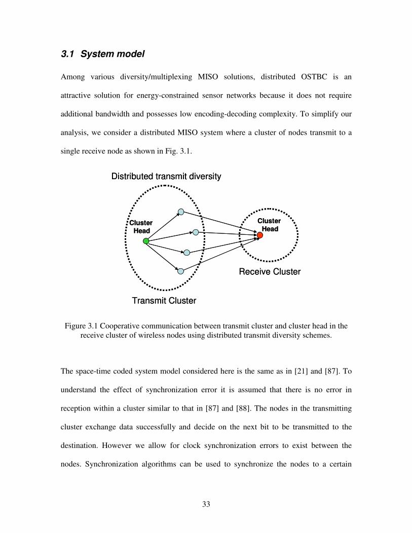
33

3.1 System model

Among various diversity/multiplexing MISO solutions, distributed OSTBC is an

attractive solution for energy-constrained sensor networks because it does not require

additional bandwidth and possesses low encoding-decoding complexity. To simplify our

analysis, we consider a distributed MISO system where a cluster of nodes transmit to a

single receive node as shown in Fig. 3.1.

Distributed transmit diversity

Cluster Head

Transmit Cluster

Cluster Head

Receive Cluster


Cluster Head

Transmit Cluster

Cluster Head

Receive Cluster

Figure 3.1 Cooperative communication between transmit cluster and cluster head in the receive cluster of wireless nodes using distributed transmit diversity schemes.

The space-time coded system model considered here is the same as in [21] and [87]. To

understand the effect of synchronization error it is assumed that there is no error in

reception within a cluster similar to that in [87] and [88]. The nodes in the transmitting

cluster exchange data successfully and decide on the next bit to be transmitted to the

destination. However we allow for clock synchronization errors to exist between the

nodes. Synchronization algorithms can be used to synchronize the nodes to a certain

34

reference or to the source node; however this requires a tradeoff between synchronization

accuracy, energy efficiency, and latency incurred during synchronization. The focus of

this paper is primarily to analyze the effect of time synchronization error on the parallel

transmission, which may help in making the aforementioned tradeoff. The effect of

imperfect intra-cluster communications on the end-to-end ABER performance of

distributed OSTBC and performance of distributed MIMO are beyond the scope of this

article but will be explored in our future work.

We consider a 2x1 MISO system where two nodes cooperate to transmit OSTBC

codewords as described in [71]. It is assumed that the channels between the distributed

transmitters and the receiver are independent (virtual transmit antennas are far apart) and

undergo frequency non-selective fading. After some rearrangement as described in [91,

eq. (5)], the received signal for coherent STBC under perfect synchronization can be

written as

,11 2

,21 12 1

ll l

ll l

sr nh hsr nh h∗ ∗∗ ∗

+ +

= + − −−

(3.1)

where lr and 1lr + are signals received during thl symbol duration and 1thl + symbol duration

respectively. ,1ls and ,2ls are the consecutive symbols that are used in forming an OSTBC

codeword. The channels are assumed to be quasi-static over the duration of the block

code. Hence, 1h and 2h represent the random channel gains from transmit antenna one and

two respectively. The channel gain can be expressed as

( )expm m mh jα θ= (3.2)

35

where mα is a random amplitude process (fading), mθ is the uniformly distributed random

phase process while ln and 1ln + are additive white Gaussian noise terms corresponding to

the received symbol durations with zero mean and a two sided power spectral density

equal to 0 2N .

( ) ( )ll

s t b g t lT∞

=−∞= − (3.3)

where lb is the thl data bit in the sequence of independent and identically distributed

binary data bits taking values 1, 1− , ( )g t is the convolution of the transmit pulse

shaping filter and the matched filter at the front end of the receiver and T is the symbol

duration. In discrete time representation, (3.3) can be written as

l ll

s b g∞

=−∞= (3.4)

The received signal at the thk symbol duration is now given by

2 2

, , . , , ,1 1

k k m k m k m l m l m l k m km m l

l k

r h b g h b g n∞

−= = =−∞

≠

= + + (3.5)

The subscript l represents the symbol sampling time while index m corresponds to the

transmit antenna from which the symbol was transmitted. The first term in (3.5) denotes

the desired signal portion while the second term corresponds to the ISI contribution and

kn denotes the AWGN noise at the input of the receiver.

36

Suppose symbol k corresponds to the start of an OSTBC block, and the receiver has

perfect channel state information for signal decoding. Hence the decision statistic at the

output of the linear combiner can be written as [91]

1 ,1 ,2

1,2 ,12

ˆ

ˆkk k

kk k

rX h hrh hX

∗

∗∗+

− = ℜ − (3.6)

Due to symmetry of the BPSK signal constellation, it will suffice to calculate the

probability of error of one of the decision statistics at the output of the linear STBC

decoder. Hence decoding the OSTBC block transmitted at thk symbol duration 1X is

given by

( ) ( )

2 2

1 ,1 ,1 ,2 1,2 ,1 ,1 ,2 ,1 ,2 ,1 1,1 ,2

2 2

,1 , , , ,2 , , 1, ,2 ,1 11 1

1

ˆ

k k k k k k k k k k k k

k l m l m l k m k l m l m l k m k k k km l m l

l k l k

X h g h g b h h g h h g b

h h b g h h b g h n h n

∗ ∗+ +

∞ ∞∗ ∗ ∗

− − − += =−∞ = =−∞

≠ ≠ +

= + + ℜ −

+ ℜ + ℜ + ℜ +

(3.7)

Notice that conjugation does not affect the binary bits, the pulse shapes or noise terms

because they are real valued.

For a known time offset error at the receiver for signals received from certain transmit

antenna, the values ,k mg are deterministic and can be compensated for. However if timing

errors cannot be compensated due to reasons discussed in section I the receiver is not

optimal and results in degraded ABER performance. In the next section we present the

frequency domain approach to evaluate the bit error probability due to pulse shaping and

time synchronization errors.

37

3.2 Frequency domain analysis

Timing error causes the bandlimited pulses of adjacent symbols received from multiple

transmit nodes to overlap at the receiver. The sources of timing errors were cited in

section I. For a SISO link they can be represented as the sum of a constant value

representing sampling offset error between transmitter and receiver and a random

variable following a Tikhonov distribution resulting from phase noise of the phase locked

loop (PLL) [108]. In the case of distributed-MISO system since we assume that accurate

timing is not achievable on all the cooperative links we characterize the combined effect

of timing error on the pulse shaped received symbol output over each link as

( ) ( ), ,l m l l ml

s t b g t lT τ∞

=−∞= − − (3.8)

where ,l mτ is modeled as a random variable uniformly distributed on ,2 2

T TU

−∆ ∆

and

0 T T≤ ∆ < . This is reasonable since an uncompensated timing offset for each

cooperative link can be allowed to fall inside a certain range and a worst case can be

assumed for phase noise in the absence of accurate PLL tracking (instantaneous loop

SNR equal to zero) in which case the Tikhonov distribution reduces to a uniform

distribution [108]. Therefore the discrete time representation of ,l mg in (3.7) can be

treated as a random variable whose outcome depends on ,l mτ where ( ), ,l m l mg g t lT τ= − − .

Without any loss of generality, let us assume that ,1 1kb = − was transmitted. In this case

(3.7) can be restated as

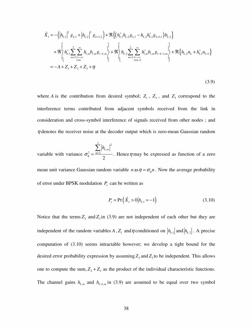
38

( ) ( )

2 2

1 ,1 ,1 ,2 1,2 ,1 ,2 ,1 ,2 ,1 1,1 ,2

2 2

,1 , , , ,2 , , 1, ,2 ,1 11 1

1

1 2 3

ˆ

k k k k k k k k k k k

k l m l m l k m k l m l m l k m k k k km l m l

l k l k

X h g h g h h g h h g b


A Z Z Z η

∗ ∗+ +

∞ ∞∗ ∗ ∗

− − − += =−∞ = =−∞

≠ ≠ +

= − + + ℜ −

+ ℜ + ℜ + ℜ +

= − + + + +

(3.9)

where A is the contribution from desired symbol; 1Z , 2Z , and 3Z correspond to the

interference terms contributed from adjacent symbols received from the link in

consideration and cross-symbol interference of signals received from other nodes ; and

η denotes the receiver noise at the decoder output which is zero-mean Gaussian random

variable with variance

2 2

,2 1

2

k mm

h

ησ ==

. Henceη may be expressed as function of a zero

mean unit variance Gaussian random variable n as nηη σ= . Now the average probability

of error under BPSK modulation eP can be written as

( )1 ,1ˆPr 0 1e kP X b= > = − (3.10)

Notice that the terms 2Z and 3Z in (3.9) are not independent of each other but they are

independent of the random variables A , 1Z andη conditioned on ,1kh and ,2kh . A precise

computation of (3.10) seems intractable however; we develop a tight bound for the

desired error probability expression by assuming 2Z and 3Z to be independent. This allows

one to compute the sum, 2 3Z Z+ as the product of the individual characteristic functions.

The channel gains ,k mh and 1,k mh + in (3.9) are assumed to be equal over two symbol

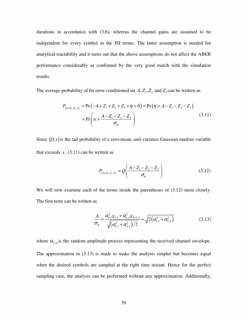
39

durations in accordance with (3.6), whereas the channel gains are assumed to be

independent for every symbol in the ISI terms. The latter assumption is needed for

analytical tractability and it turns out that the above assumptions do not affect the ABER

performance considerably as confirmed by the very good match with the simulation

results.

The average probability of bit error conditioned on 1 2 3, , and A Z Z Z can be written as

( ) ( )1 2 3 1 2 3 1 2 3, , ,

1 2 3

Pr 0 Pr

Pr

e A Z Z ZP A Z Z Z A Z Z Z

A Z Z Zn

η

η η

σ

= − + + + + > = > − − −

− − −= >

(3.11)

Since ( )Q x is the tail probability of a zero-mean, unit variance Gaussian random variable

that exceeds x , (3.11) can be written as

1 2 3

1 2 3, , ,e A Z Z Z

A Z Z ZP Q

ησ − − −=

(3.12)

We will now examine each of the terms inside the parentheses of (3.12) more closely.

The first term can be written as

( )

( )2 2,1 ,1 ,2 1,2 2 2

,1 ,22 2,1 ,2

22

k k k kk k

k k

g gA

η

α αα α

σ α α++

= ≈ ++

(3.13)

where ,k mα is the random amplitude process representing the received channel envelope.

The approximation in (3.13) is made to make the analysis simpler but becomes equal

when the desired symbols are sampled at the right time instant. Hence for the perfect

sampling case, the analysis can be performed without any approximation. Additionally,

40

the above approximation for the imperfect sampling case however does not significantly

affect the ABER performance curves.

The second term can be written as

( ) ( )

( ) ( ),1 ,2 ,2 ,2 ,1 1,1 ,2 ,1 ,2 ,1 ,21

12 2 2 2,1 ,2 ,1 ,2

cos0

2 2

k k k k k k k k k k k

k k k k

g g bZI

η

α α α α θ θ α ασ α α α α

+− −= = ≈

+ +(3.14)

where ( ) ( )1 ,2 1,1 ,2 ,1 ,2cosk k k k kI g g b θ θ+= − − is a random variable which is the of the

product of real independent random variables and ,k mθ is the random phase associated

with the fading process which is considered to be uniformly distributed between [ ],π π− .

In particular, the approximation holds when ,2 1,1 0k kg g +− ≈ . We observe that the

contribution of this ISI term is very small and can be ignored for all practical purposes. It

should be noted that our analysis can still capture the effect of the above term at slightly

higher computational cost.

The third term can be expressed as

( )

( ) ( )

2

,1 , , ,1 , ,1

,122

2 2 2 2,1 ,2 ,1 ,2

cos

2 2

k l m l m k l m k l mm l

l k k

k k k k

b gZ

Iη

α α θ θα

σ α α α α

∞

−= =−∞

≠

−

= =+ +

(3.15)

where ( )2

2 , , ,1 , ,1

cosl m l m k l m k l mm l

l k

I b gα θ θ∞

−= =−∞

≠

= − is a random variable which is the result of

the sum of the product of real independent random variables. The fourth term in the

argument of (3.12) can be similarly written as

41

( )

( ) ( )

2

,2 , , ,2 , 1,1

1 ,233

2 2 2 2,1 ,2 ,1 ,2

cos

2 2

k l m l m k l m l k mm l

l k k

k k k k

b gZ

Iη

α α θ θα

σ α α α α

∞

− −= =−∞

≠ +

−

= =+ +

(3.16)

where ( )2

3 , , ,2 , 1,1

1

cosl m l m k l m l k mm l

l k

I b gα θ θ∞

− −= =−∞

≠ +

= − . Based on our assumptions, the four

terms in the argument of (3.12) are independent of each other conditioned on ,1kα and ,2kα .

Now utilizing an alternate integral representation for the Gaussian probability integral

[84]

( ) 2 2

0

1 1 12

t jtxQ x e e dttπ

∞− −= + ℑ (3.17)

It is possible to average the random variables identified in (3.13)-(3.16) to get desired

ABER in terms of a triple integral, viz,

( ) ( ) ( ) ( ) ( )

( )

2

,1 ,2 3 2 1

2 2,1 ,2 ,1 ,22 2

,1 ,1 1 2 32 2 2 22 2,1 ,1 ,1 ,1,1 ,2

2,1 ,2 3 2 1

0 0 0

22

1 2 3 ,

1 1 12

k k

k k k kk k

k k k kk k

te k k I I I

jt I I I

k

P e f f f I f I f It

e dI dI dI d

α α

α α α αα α

α α α αα α

α απ

α

∞ ∞ ∞ ∞ ∞ ∞−

−∞ −∞ −∞

− + + + + + + +

= + ℑ

×

( ) ( ) ( )2 22 ,1 ,1

,1 ,2

1 2 3

2 ,1

22,1 ,2

0 0 0

2 2,1 ,2 ,1 ,2

1 2 3 ,2 ,12 2 2 2 2 2,1 ,1 ,1 ,1 ,1 ,1

1 1 1

2

2 2 2

k k

k k

k

jttk k

k k k kI I I k k

k k k k k k

d dt

e f f et

I I I d d dt

α α

α α

α

α απ

α α α αφ φ φ α α

α α α α α α

∞ ∞ ∞ − +− = + ℑ

× + + +

(3.18)

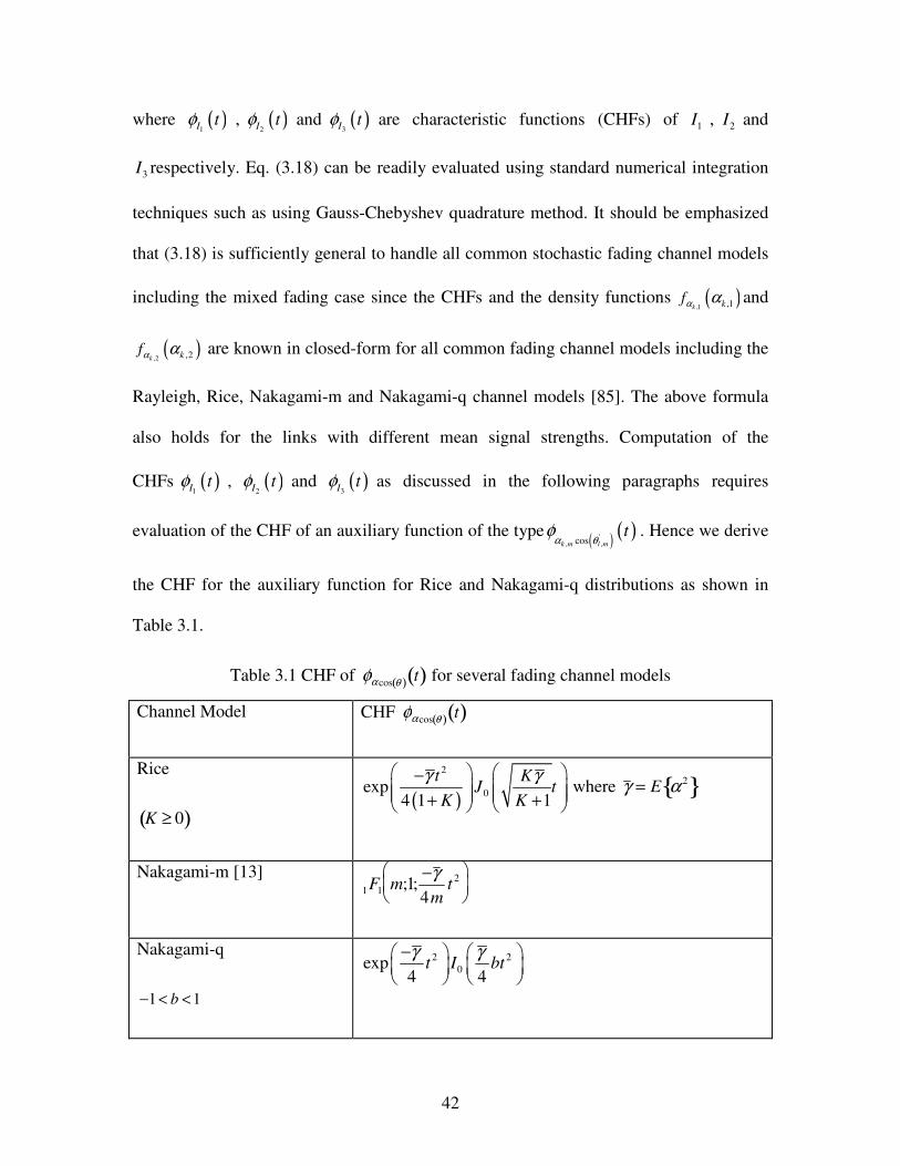
42

where ( )1I

tφ , ( )2I tφ and ( )

3I tφ are characteristic functions (CHFs) of 1I , 2I and

3I respectively. Eq. (3.18) can be readily evaluated using standard numerical integration

techniques such as using Gauss-Chebyshev quadrature method. It should be emphasized

that (3.18) is sufficiently general to handle all common stochastic fading channel models

including the mixed fading case since the CHFs and the density functions ( ),1 ,1k kfα α and

( ),2 ,2k kfα α are known in closed-form for all common fading channel models including the

Rayleigh, Rice, Nakagami-m and Nakagami-q channel models [85]. The above formula

also holds for the links with different mean signal strengths. Computation of the

CHFs ( )1I

tφ , ( )2I tφ and ( )

3I tφ as discussed in the following paragraphs requires

evaluation of the CHF of an auxiliary function of the type ( ) ( )', ,cosk m l m

tα θ

φ . Hence we derive

the CHF for the auxiliary function for Rice and Nakagami-q distributions as shown in

Table 3.1.

Table 3.1 CHF of φα cos θ( ) t( ) for several fading channel models

Channel Model CHF φα cos θ( ) t( )

Rice

K ≥ 0( ) ( )

2

0exp4 1 1

t KJ t

K Kγ γ −

+ + where γ = E α 2

Nakagami-m [13] 1F1 m;1;

−γ 4m

t 2

Nakagami-q

1 1b− < <

2 20exp

4 4t I bt

γ γ−

43

The following well known property for the CHF involving a product of two real and

independent random variables will be applied to derive the required CHF.

If X and Y are two independent real random variables with characteristic functions φ and

ψ respectively. The product XY has characteristic function is given by

( ) ( ) jtXYY X X YE e E tY E tXφ ψ= = (3.19)

Since

( ) ( ) ( ) jtXY jtXy jtXyX y X y X YE e E e Y y f y dy E e f y dy E tXψ

∞ ∞

−∞ −∞

= = = =

(3.20)

Applying (3.19) to compute ( )1I

tφ we obtain

( ) ( ) ( ) ( ) ( ) ( )( )

( )( ) ( )( )

'1 ,2 1,1 ,2,2 1,1 ,2 ,1 ,2 ,1 2,2 ,2 1,1cos cos

2 2

0 ,2 1,1 0 ,2 1,1 1,1 ,22 2

1 1 0.5 0.5

k k kk k k k k kI b k k kg g b

T T

k k k k k kT T

t t E E E tb g g

J t g g J t g g d dT T

τ τθ θ θφ φ φ

τ τ

++ −+− −

∆ ∆

+ + +−∆ −∆

= = −

= − − + − ∆ ∆ (3.21)

where timing errors ,2kτ and 1,1kτ + , that affect the sampled values of the pulse shapes

,2kg and 1,1kg + respectively, are assumed to be uniformly distributed over ,2 2

T T−∆ ∆

.

The notation 0J represents a zero-order Bessel function of the first kind. Note that

when ,2 1,1 0k kg g +− = , the CHF ( )1

1I tφ = .

Similarly applying (3.19) in computation of ( )2I tφ we obtain

( )( )

( ) ( ) ( ) 2 '2 , ,' , ,, , , ,

1

2

, ,coscos 1

0

l m l m k m l mk m l m l m k l m

m ll k

p

I b l m l mb g m l p

p

t t E E tb gτ α θα θφ φ φ∞

−= =−∞

≠

= =−≠

= =

∏∏ (3.22)

44

where ', , ,1l m l m kθ θ θ= − and the ISI is restricted to 2 p adjacent symbols. The CHF

( ) ( )', ,cosk m l m

tα θ

φ can be evaluated using [83, Eq. (36)-(42)]. It should be noted; however [83]

only evaluated the CHF for Nakagami-m fading. We have derived closed form

expressions for CHF ( ) ( )', ,cosk m l m

tα θ

φ for Rice and Nakagami-q channels with the aid of [86

Eq. (6.3334)] and [86 Eq. (6.6516)] in Table 1. For uniform distribution of timing error,

over ,2 2

T T−∆ ∆

, the expression in (3.22) can be written as

( ) ( ) ( ) ( ) ( )' '2 , , , ,

22

, , ,cos cos1 2

0

10.5 0.5

k m l m k m l m

Tp

I l m l m l mm l p T

l

t tg tg dT α θ α θ

φ φ φ τ∆

= =− −∆≠

= − + − ∆∏∏ (3.23)

( )3I tφ can be computed in a similar fashion and the final result is given by

( ) ( ) ( ) ( ) ( )' '3 , 1, , 1,

22

1, 1, 1,cos cos1 2

1

10.5 0.5

k m l m k m l m

Tp

I l m l m l mm l p T

l

t tg tg dT α θ α θ

φ φ φ τ+ +

∆

+ + += =− −∆

≠

= − + − ∆∏∏ (3.24)

Notice that these expressions accommodate distributed links with non-identical family of

distributions as well as non-identical channel gains. In section V we also compare our

analytical results with simulation. The validation of our analytical results and its

application are discussed in section V.

3.3 Extension to distributed 1Ν × MISO networks

In the preceding sections, we have discussed the system model and analysis for a

distributed 2 1× MISO system with orthogonal STBC scheme. Our approach can be

extended to handle a more general class of 1N × distributed MISO networks as well (i.e.

more than two cooperating nodes in the transmit cluster). The physical layer operations

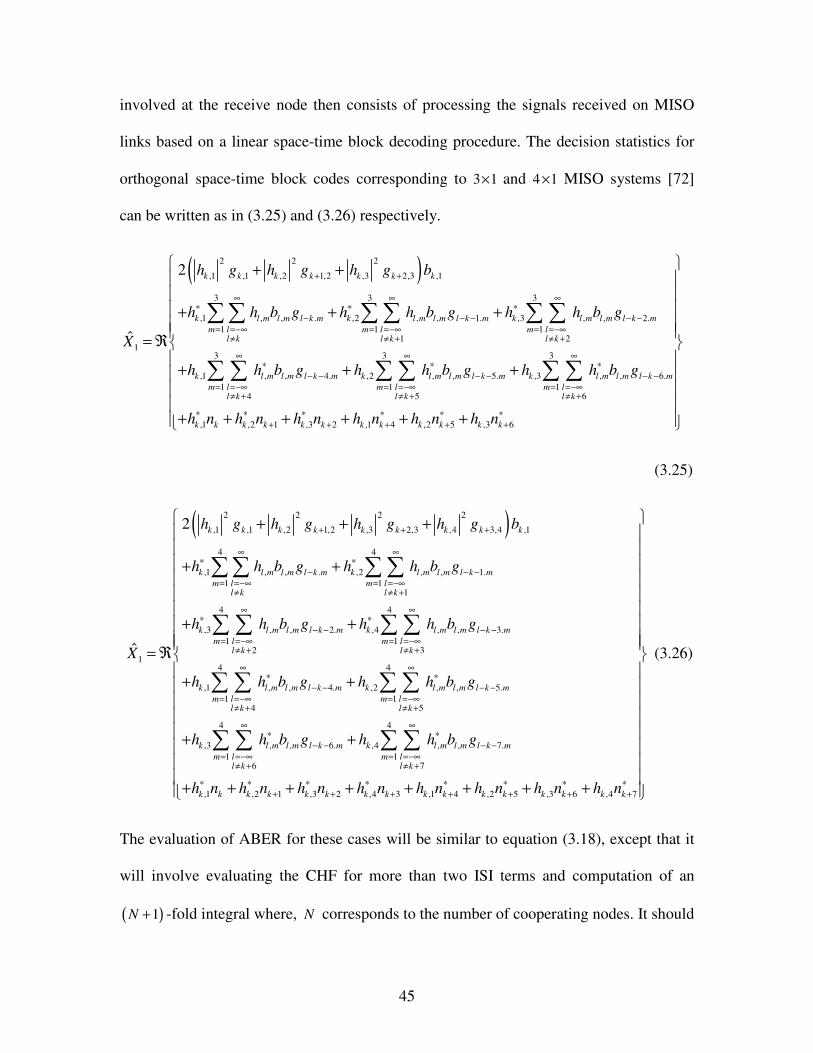
45

involved at the receive node then consists of processing the signals received on MISO

links based on a linear space-time block decoding procedure. The decision statistics for

orthogonal space-time block codes corresponding to 3 1× and 4 1× MISO systems [72]

can be written as in (3.25) and (3.26) respectively.

( )2 2 2

,1 ,1 ,2 1,2 ,3 2,3 ,1

3 3 3

,1 , , . ,2 , , 1. ,3 , , 2.1 1 1

1 21

3

,1 , , 4. ,2 ,1

4

2

ˆ

k k k k k k k

k l m l m l k m k l m l m l k m k l m l m l k mm l m l m l

l k l k l k

k l m l m l k m k l mm l

l k

h g h g h g b

h h b g h h b g h h b g

X

h h b g h h

+ +

∞ ∞ ∞∗ ∗ ∗

− − − − −= =−∞ = =−∞ = =−∞

≠ ≠ + ≠ +

∞∗

− −= =−∞

≠ +

+ +

+ + +

= ℜ

+ +

3 3

, 5. ,3 , , 6.1 1

5 6

,1 ,2 1 ,3 2 ,1 4 ,2 5 ,3 6

l m l k m k l m l m l k mm l m l

l k l k

k k k k k k k k k k k k

b g h h b g

h n h n h n h n h n h n

∞ ∞∗ ∗

− − − −= =−∞ = =−∞

≠ + ≠ +

∗ ∗ ∗ ∗ ∗ ∗+ + + + +

+

+ + + + + +

(3.25)

( )2 2 2 2

,1 ,1 ,2 1,2 ,3 2,3 ,4 3,4 ,1

4 4

,1 , , . ,2 , , 1.1 1

1

4

,3 , , 2. ,4 , , 3.1

2 31

2

ˆ

k k k k k k k k k

k l m l m l k m k l m l m l k mm l m l

l k l k


l k l k

h g h g h g h g b

h h b g h h b g

h h b g h h b g

X

+ + +

∞ ∞∗ ∗

− − −= =−∞ = =−∞

≠ ≠ +

∞ ∞∗ ∗

− − − −= =−∞ = =−∞

≠ + ≠ +

+ + +

+ +

+ +

= ℜ

4

1

4 4

,1 , , 4. ,2 , , 5.1 1

4 5

4 4

,3 , , 6. ,4 , , 7.1 1

6 7

,1 ,2 1 ,3 2 ,4 3 ,1


l k l k


l k l k

k k k k k k k k k k

h h b g h h b g

h h b g h h b g

h n h n h n h n h n

∞ ∞∗ ∗

− − − −= =−∞ = =−∞

≠ + ≠ +

∞ ∞∗ ∗

− − − −= =−∞ = =−∞

≠ + ≠ +

∗ ∗ ∗ ∗+ + +

+ +

+ +

+ + + + +

4 ,2 5 ,3 6 ,4 7k k k k k kh n h n h n∗ ∗ ∗ ∗+ + + +

+ + +

(3.26)

The evaluation of ABER for these cases will be similar to equation (3.18), except that it

will involve evaluating the CHF for more than two ISI terms and computation of an

( )1N + -fold integral where, N corresponds to the number of cooperating nodes. It should

46

be noted that for block lengths greater than two the orthogonal STBC schemes achieve

code rates less than 1 and hence may require use of higher order constellation for proper

comparison.

3.4 Computational results

In this section, we will present selected numerical results to highlight the applications of

our analytical framework for characterizing the performance of distributed orthogonal

STBC subject to timing synchronization errors under different fading environments as

well as different choices of pulse shaping filters. Fig. 3.2 and Fig. 3.3 plots both the

analytical and simulation results for the ABER of a 2x1 distributed OSTBC system in

Rayleigh and Nakagami-m fading channels for different values of timing synchronization

errors (uniformly distributed between ,2 2

T T−∆ ∆

). For the Monte Carlo simulation we

follow the system described in (3.9). It is assumed that the channel remains constant for

the duration of two symbols that corresponds to the length of the space-time block. In

contrast to the analysis the interfering terms 2Z and 3Z are not independent in the

simulation. The timing errors are uniformly distributed as considered for analysis. The

average channel received SNR on both links are identical i.e.; the total received SNR is

equally distributed across both links. Raised cosine pulse shaping is employed with a roll-

off factor of 0.22α = . The figures verify the validity of the analysis presented in section

III. The performance curves obtained via our analytical approach are in good agreement

with that of Monte Carlo simulation results.

It can be observed from Fig. 3.2 that as the timing error increases the ABER performance

degrades rapidly. However the performance of distributed OSTBC system, even with

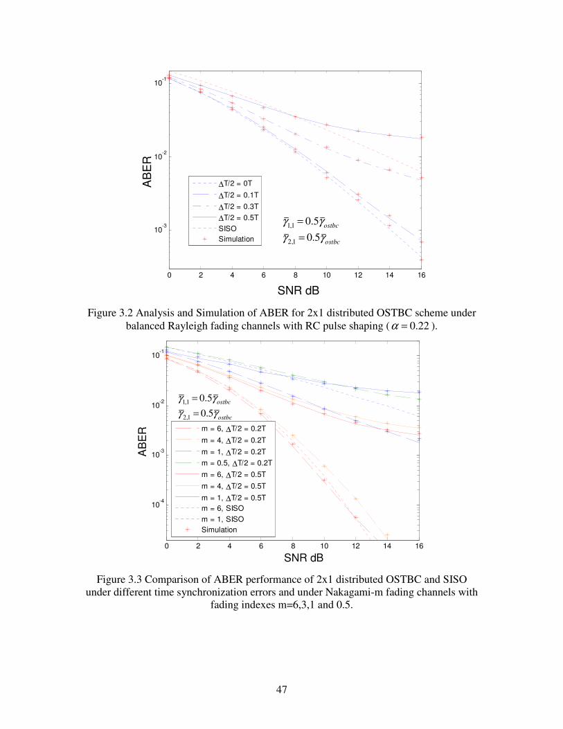
47

0 2 4 6 8 10 12 14 16

10-3

10-2

10-1

∆T/2 = 0T

∆T/2 = 0.1T

∆T/2 = 0.3T

∆T/2 = 0.5TSISOSimulation

AB

ER

SNR dB

1,1

2,1

0.50.5

ostbc

ostbc

γ γγ γ

==

Figure 3.2 Analysis and Simulation of ABER for 2x1 distributed OSTBC scheme under

balanced Rayleigh fading channels with RC pulse shaping ( 0.22α = ).

0 2 4 6 8 10 12 14 16

10-4

10-3

10-2

10-1

m = 6, ∆T/2 = 0.2T

m = 4, ∆T/2 = 0.2Tm = 1, ∆T/2 = 0.2Tm = 0.5, ∆T/2 = 0.2Tm = 6, ∆T/2 = 0.5Tm = 4, ∆T/2 = 0.5T

m = 1, ∆T/2 = 0.5Tm = 6, SISOm = 1, SISOSimulation

AB

ER

SNR dB

1,1

2,1

0.50.5

ostbc

ostbc

γ γγ γ

==

Figure 3.3 Comparison of ABER performance of 2x1 distributed OSTBC and SISO

under different time synchronization errors and under Nakagami-m fading channels with fading indexes m=6,3,1 and 0.5.

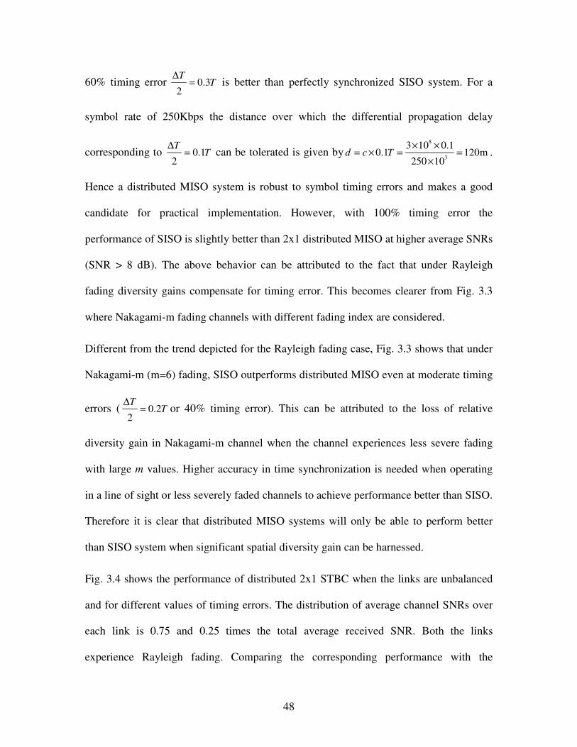
48

60% timing error 0.32

TT

∆= is better than perfectly synchronized SISO system. For a

symbol rate of 250Kbps the distance over which the differential propagation delay

corresponding to 0.12

TT

∆= can be tolerated is given by

8

3

3 10 0.10.1 120m

250 10d c T

× ×= × = =

×.

Hence a distributed MISO system is robust to symbol timing errors and makes a good

candidate for practical implementation. However, with 100% timing error the

performance of SISO is slightly better than 2x1 distributed MISO at higher average SNRs

(SNR > 8 dB). The above behavior can be attributed to the fact that under Rayleigh

fading diversity gains compensate for timing error. This becomes clearer from Fig. 3.3

where Nakagami-m fading channels with different fading index are considered.

Different from the trend depicted for the Rayleigh fading case, Fig. 3.3 shows that under

Nakagami-m (m=6) fading, SISO outperforms distributed MISO even at moderate timing

errors ( 0.22

TT

∆= or 40% timing error). This can be attributed to the loss of relative

diversity gain in Nakagami-m channel when the channel experiences less severe fading

with large m values. Higher accuracy in time synchronization is needed when operating

in a line of sight or less severely faded channels to achieve performance better than SISO.

Therefore it is clear that distributed MISO systems will only be able to perform better

than SISO system when significant spatial diversity gain can be harnessed.

Fig. 3.4 shows the performance of distributed 2x1 STBC when the links are unbalanced

and for different values of timing errors. The distribution of average channel SNRs over

each link is 0.75 and 0.25 times the total average received SNR. Both the links

experience Rayleigh fading. Comparing the corresponding performance with the

49

balanced case it can be observed that the balanced case outperforms the unbalanced case

by 2 dB when 0.32

TT

∆= at ABER of 210− . Since the best performance is achieved when

the links are balanced, an optimal strategy may be used to achieve better performance

subject to total power constraint.

0 2 4 6 8 10 12 14 1610

-4

10-3

10-2

10-1

100

∆T/2 = 0.1T

∆T/2 = 0.3T

∆T/2 = 0.5T

AB

ER

SNR dB

1,1

2,1

0.750.25

ostbc

ostbc

γ γγ γ

==

Figure 3.4 ABER for 2x1 distributed OSTBC scheme under unbalanced Rayleigh fading

channels with RC pulse shaping ( 0.22α = ).

In Fig. 3.5 we plot the ABER performance of distributed MISO for the case where the

two cooperative links undergo fading from two different families of distribution. This

allows for investigation of the effect of fading parameter on ISI. Specifically we choose a

case where one of the links is lightly faded (Nakagami-m with m = 6) and the other link

with a different family of distribution corresponding to a different fading parameter. Two

reference cases where both links undergo Rayleigh and Nakagami-m (m=6) respectively

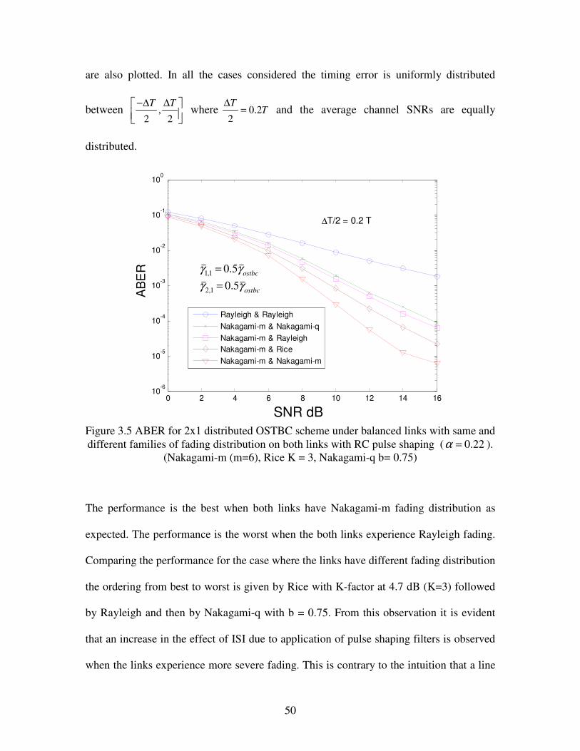
50

are also plotted. In all the cases considered the timing error is uniformly distributed

between ,2 2

T T−∆ ∆

where 0.22

TT

∆= and the average channel SNRs are equally

distributed.

0 2 4 6 8 10 12 14 1610

-6

10-5

10-4

10-3

10-2

10-1

100

Rayleigh & RayleighNakagami-m & Nakagami-qNakagami-m & RayleighNakagami-m & RiceNakagami-m & Nakagami-m

∆T/2 = 0.2 T

AB

ER

SNR dB

1,1

2,1

0.50.5

ostbc

ostbc

γ γγ γ

==

Figure 3.5 ABER for 2x1 distributed OSTBC scheme under balanced links with same and different families of fading distribution on both links with RC pulse shaping ( 0.22α = ).

(Nakagami-m (m=6), Rice K = 3, Nakagami-q b= 0.75)

The performance is the best when both links have Nakagami-m fading distribution as

expected. The performance is the worst when the both links experience Rayleigh fading.

Comparing the performance for the case where the links have different fading distribution

the ordering from best to worst is given by Rice with K-factor at 4.7 dB (K=3) followed

by Rayleigh and then by Nakagami-q with b = 0.75. From this observation it is evident

that an increase in the effect of ISI due to application of pulse shaping filters is observed

when the links experience more severe fading. This is contrary to the intuition that a line

51

of sight link with the same average power would cause more ISI. One plausible

explanation is given in [92]. It is shown in [92] that when the noise due to interference is

Gaussian and the probability of error is a Q -function that is concave-up, larger

interference always results in higher probability of error. However if the complementary

function for calculating the probability of error is concave-down then the reverse may be

true. It was further predicted that this will be caused when the noise has a density

function with more than one bump or in a communication system with a different

signaling and detection strategy. Now if we consider the case where AWGN is absent and

only ISI is present then the complementary function is the Laplace inverse transform of

CHF given in equation (3.30) which in turn depends on ( ) ( )', ,cosk m l m

tα θ

φ . Fig. 1 in [83] gives

the PDF of ( ) ( )', ,cosk m l m

tα θ

φ for different fading severity indexes for Nakagami-m fading

distribution. It can clearly be seen that as the fading severity decreases for increasing

values of m, the PDF has multiple bumps confirming the behavior of ABER performance

under ISI for less severely faded links.

Fig. 3.6 shows the performance of distributed 2x1 MISO links under Nakagami-m (m=6)

and Rayleigh fading distributions respectively under different average channel SNR

distribution and timing error uniformly distributed between ,2 2

T T−∆ ∆

where 0.22

TT

∆= .

Three cases are considered. In the first case the Rayleigh faded link has lesser average

channel SNR (0.25 time the total channel SNR) than the Nakagami-m faded link (0.75

time the total channel SNR). The second case has balanced distribution and the third case

where the distribution is the reverse of the first case. It can be seen that the best

performance is observed when the Nakagami-m faded link has higher average channel

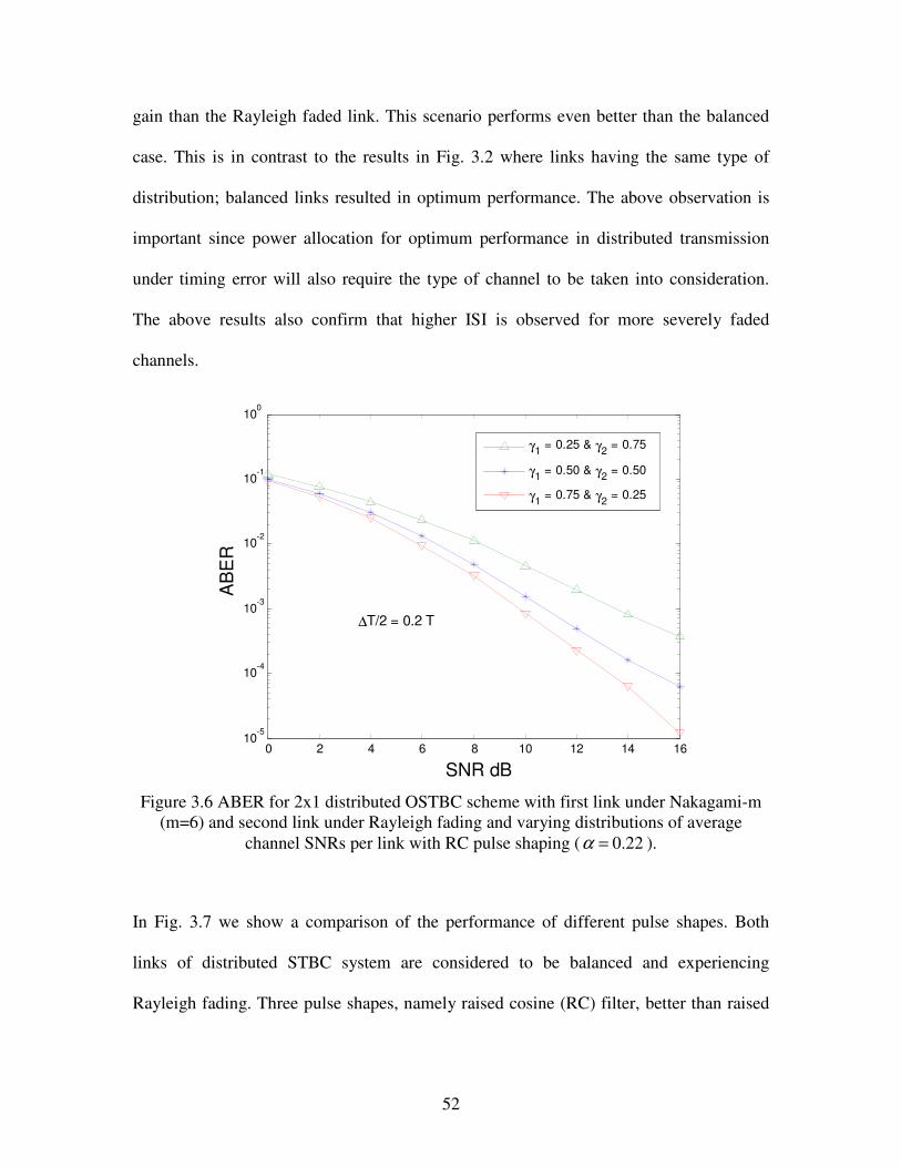
52

gain than the Rayleigh faded link. This scenario performs even better than the balanced

case. This is in contrast to the results in Fig. 3.2 where links having the same type of

distribution; balanced links resulted in optimum performance. The above observation is

important since power allocation for optimum performance in distributed transmission

under timing error will also require the type of channel to be taken into consideration.

The above results also confirm that higher ISI is observed for more severely faded

channels.

AB

ER

SNR dB0 2 4 6 8 10 12 14 16

10-5

10-4

10-3

10-2

10-1

100

γ1 = 0.25 & γ2 = 0.75

γ1 = 0.50 & γ2 = 0.50

γ1 = 0.75 & γ2 = 0.25

∆T/2 = 0.2 T

Figure 3.6 ABER for 2x1 distributed OSTBC scheme with first link under Nakagami-m

(m=6) and second link under Rayleigh fading and varying distributions of average channel SNRs per link with RC pulse shaping ( 0.22α = ).

In Fig. 3.7 we show a comparison of the performance of different pulse shapes. Both

links of distributed STBC system are considered to be balanced and experiencing

Rayleigh fading. Three pulse shapes, namely raised cosine (RC) filter, better than raised

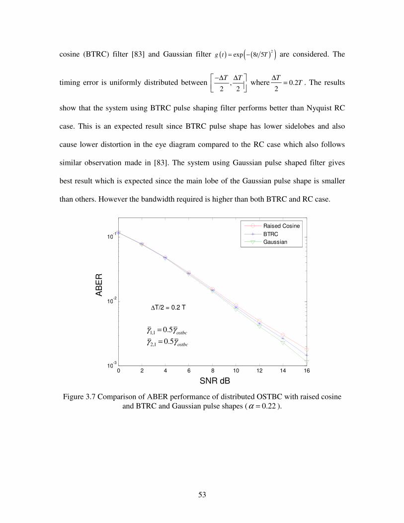
53

cosine (BTRC) filter [83] and Gaussian filter ( ) ( )( )2exp 8 5g t t T= − are considered. The

timing error is uniformly distributed between ,2 2

T T−∆ ∆

where 0.22

TT

∆= . The results

show that the system using BTRC pulse shaping filter performs better than Nyquist RC

case. This is an expected result since BTRC pulse shape has lower sidelobes and also

cause lower distortion in the eye diagram compared to the RC case which also follows

similar observation made in [83]. The system using Gaussian pulse shaped filter gives

best result which is expected since the main lobe of the Gaussian pulse shape is smaller

than others. However the bandwidth required is higher than both BTRC and RC case.

0 2 4 6 8 10 12 14 1610

-3

10-2

10-1

Raised CosineBTRCGaussian

∆T/2 = 0.2 T

AB

ER

SNR dB

1,1

2,1

0.50.5

ostbc

ostbc

γ γγ γ

==

Figure 3.7 Comparison of ABER performance of distributed OSTBC with raised cosine

and BTRC and Gaussian pulse shapes ( 0.22α = ).

54

3.5 Conclusions

In this chapter, we presented an efficient method for evaluating the ABER performance

of distributed space time coded systems subjected to time synchronization errors.

Numerical results show that time synchronization errors in a bandlimited distributed

OSTBC system degrades the ABER performance rapidly with increasing timing jitter.

However it was observed that for timing errors less than 60% a distributed OSTBC

system can still outperform perfectly synchronized SISO when there is enough diversity

gain available (i.e. in severe fading environments). It was observed that effect of ISI due

to timing errors in a distributed OSTBC system is more pronounced under severely faded

links compared to less severely faded links. Under non-identically distributed channels

with different average channel gains, having more power allocated to a less faded link

gives better performance than the balanced scenario.

From the above observations it appears that under certain channel conditions with

reduced overhead on node synchronization distributed OSTBC can outperform a SISO

system. However for conditions (e.g. under line of sight) where the system does not

provide significant improvements over a SISO system under timing errors one may have

to look at alternate designs for cooperative communication that combat synchronization

errors. For example design of space-time codes that are resilient to timing errors [109],

[110] or explore transceiver designs for cooperative communication that operate under

asynchronous transmission [111].

55

Chapter 4

4 Node density and range improvement in cooperative networks using randomized STBC

In the previous chapters we looked at performance improvements in terms of outage and bit error

rate. In this chapter we consider the benefits of cooperative transmission in terms of range

improvement. Distributed beamforming [62] is one of the ways to improve range. However due

to the nature of the physical distribution of the nodes co-phasing of the transmitted signals can be

a daunting challenge. Hence in this chapter we investigate range improvement with cooperative

diversity. Previous work in [93], described a new transmission scheme for cooperative

communication, called randomized orthogonal space-time block coding (OSTBC), that allows

each node to randomly choose and transmit one column of a given space-time code matrix. It

was shown in [93] that this scheme achieves maximum possible diversity order for a given SNR

as the number of cooperating nodes increases. When nodes cooperate the total transmitted power

per symbol is also larger. Intuitively larger transmission power should result in improved range.

However, presence of time synchronization errors can limit the range that can be achieved. Time

synchronization errors especially in a distributed set up like cooperative communication can arise

due to various factors, which have already been discussed in chapter 4. Hence in this chapter we

try to examine the relationship between node density and range improvement in cooperative

communication under timing error for the signaling scheme described in [93]. We use the

Gaussian approximation to evaluate the SINR at the receiver and then evaluate the corresponding

range improvement. We show that the scaling of range as the number of nodes increase is not

56

linear. For a given amount of timing error, the range increase reaches a limit after which

increasing the number of nodes does not improve the range.

4.1 System model

We consider a distributed MISO system where a cluster of nodes transmit to a single receive

node as shown in Fig. 4.1. Further it is assumed that the nodes in the transmitting cluster are able

to exchange data and coordinate among themselves in an error free high SNR mode. A source

transmits information to other nodes within the transmit cluster which then encode the symbols

using randomized STBC scheme and relay them to the receiver.


Cluster Head

Transmit Cluster

Cluster Head

Receive Cluster

Figure 4.1 Cooperative MISO transmission

The randomized STBC scheme is explained as follows. Assume an orthogonal space-time block

code matrix G with dimensions p M× where p is the number of time slots used during

transmission of the code block and M is the number of columns. Let NT be the total number of

cooperating nodes in the transmit cluster then, a group of mN nodes may choose to transmit the

thm column of G where

Nm

m=1

M

= NT

. Orthogonal code matrix is chosen since it allows the code to

maintain diversity benefits even when one of the columns is not transmitted [93].

A BPSK system is considered where the received signal at the destination can be written as

57

G= +r h n (4.1)

where [ ]1 2T

Mh h h=h and

hm = hm,i

i=1

Nm

(4.2)

corresponds to the equivalent channel coefficient seen by the receiver corresponding to thm

column of code matrix transmitted by mN nodes. It is also assumed that the channels between the

distributed transmitters and the receiver are independent and undergo slow frequency non-

selective fading. ( )00,CN Nn I is AWGN noise at the receiver. To enhance the understanding of

the effect of pulse shaping on the performance of range we limit our analysis to the 2x2

orthogonal block code matrix also known as Alamouti’s space-time coding scheme [71]. In this

case 2M = . However this can easily be extended to other block lengths 2M > .

The pulse shaped symbol at the output of the receiver in the absence of noise and fading,

corresponding to one of the transmitting antennas can be expressed as

( ) ( )ll

s t b g t lT∞

=−∞= − (4.3)

where lb is an independent random variable that represents transmitted binary data sequence

taking values 1, 1− with equal probabilities. ( )g t is the output at the receiver of the pulse

shaped waveform used for symbol transmission and T is the symbol duration. In discrete form

equation (4.3) can be written as

l ll

s b g∞

=−∞= (4.4)

The received signal block starting at thk symbol time duration is now given by

58

2

, , . , , ,1 1

21 1

, 1, 1. , , 1,1 1

1

T

T

N

k m k m k m l j l j l k jm j l

l kk k

Nk k

k m k m k m l j l j l k jm j l

l k

h b g h b gr n

r nh b g h b g

∞

−= = =−∞

≠∗∞

+ ++ + − −

= = =−∞≠ +

+

= + +

(4.5)

The subscripts k and l represent the symbol sampling time. ,k mh represents mh , the equivalent

channel coefficient, at the thk symbol duration as defined earlier in (4.1). ,l jh is the channel

coefficient corresponding to the thl time duration transmitted from the thj transmit antenna.

Hence the desired portion of the received signal at thk symbol duration is given by

2

, , , .1

k desired k m k m k mm

r h b g=

= (4.6)

Here we make an assumption that the main lobe of the pulse shaped symbol is sampled at the

center and hence (4.6) can be rewritten as

2

, , ,1

k desired k m k mm

r h b=

≈ (4.7)

This assumption does not have much effect on performance results, which have been confirmed

through simulations. Now the ISI portion of the received signal is given by

, , , ,1

TN

k isi l j l j l k jj l

l k

r h b g∞

−= =−∞

≠

= (4.8)

It is assumed that the receiver is able to correctly estimate the equivalent channel coefficient for

a column of block code transmitted through the transmission of preambles. Hence the decision

statistic at the output of the linear combiner can be written as [91]

59

1 ,1 ,2

1,2 ,12

ˆ

ˆkk k

kk k

rX h hrh hX

∗

∗∗+

− = ℜ − (4.9)

Due to symmetry considerations of the BPSK system, it will suffice to calculate one of the

decision statistics at the output of the linear combiner. Therefore we choose 1X which is given

by

2

, , , , ,1 1

1 ,1 ,2 2

, 1, 1, , 1, 11 1

1

ˆ

T

T

N

k m k m l j l j l k j km j l

l k

k k N

k m k m l j l j l k j km j l

l k

h b h b g n

X h h

h b h b g n

∞

−= = =−∞

≠∗

∞∗ ∗

+ + − − += = =−∞

≠ +

+ +

= ℜ − − − −

(4.10)

Decoding the OSTBC block transmitted for thk symbol time duration; equation (4.9) becomes

( ) ( )

2 2

1 ,1 ,2 ,1 ,1 ,2 ,2 ,1 ,2

,1 , , . ,2 , , 1, ,2 ,1 11 1

1

1 2 1 2

ˆ

T T

k k k k k k k k

N N

k l j l j l k j k l j l j l k j k k k kj l j l

l k l k

X h h b h h h h b


X X Z Z η

∗ ∗

∞ ∞∗ ∗ ∗

− − − += =−∞ = =−∞

≠ ≠ +

= + + ℜ −

+ ℜ + ℜ + ℜ +

= + + + +

(4.11)

where 1X is the desired part, 2 0X ≈ , 1Z and 2Z are ISI terms and η corresponds to the receiver

noise at the decoder output. Next we evaluate the SINR due to ISI resulting from timing errors

by applying Gaussian approximation.

4.2 SINR using Gaussian Approximation

The Gaussian random variable η has a mean equal to zero and its variance is given by

60

22,

2 1

2

k mm

E

η

ασ ==

(4.12)

where ,k mα is the amplitude process corresponding to ,k mh . From (4.2) the PDF of ,k mh can be

approximated as ( )20, iCN σ for large values of iN where 2

1

iN

i ii

σ γ=

= and iγ is the average received

channel SNR for signal transmitted from thi node. Hence (4.12) can be rewritten as

2 1

2

TN

ii

η

γσ ==

(4.13)

Gaussian approximation estimates the ISI terms 1Z and 2Z as Gaussian random variables with a

certain mean and variance. 2Z can be expressed as

( )1 ,1 , , ,1 , ,1

cosTN

k k j l j k l j l k jj l

l k

Z b gα α θ θ∞

−= =−∞

≠

= − (4.14)

and 2Z as

( )2 ,2 , , ,1 , ,1

1

cosTN

k l j l j k l j l k jj l

l k

Z b gα α θ θ∞

−= =−∞

≠ +

= − (4.15)

From (4.13) and (4.14) it can be seen that the expected values of 1Z and 2Z are zero. Hence the

mean for all the ISI terms are zero. The variance of 1Z can be calculated as follows:

( ) ( ) ( )( ) ( ) ( )

( ) ( )

1

22 2 222 ',,1 , , ,

1

2 2,1 , ,

1 1 1

cos

1 1 1 1

2 2

T

mT T

N

l jZ k l j l j l k jj l

l k

lT lTNN N

k l j i l jj l i j llT lT

l k l k

E E E E b E g

g t dt g t dtτ τ

σ α α θ

γτ τ

∞

−= =−∞

≠

+ +∞ ∞

= =−∞ = = =−∞≠ ≠

=

= Ω Ω − = Ω −

(4.16)

61

Similarly the variance of 2Z can be computed as

( ) ( )2

2 2 2,2 , ,

1 1 1

1 1 1 12 2

T mT TlT lTN NN N

Z k l j i l jj l i j llT lT

l k l k

g t dt g t dtτ τ

σ γτ τ

+ +−∞ ∞

= =−∞ = = =−∞≠ ≠

= Ω Ω − = Ω −

(4.17)

Adding the variances computed for noise term in (4.12) and the variances in (4.15) and (4.16),

one can now compute the SINR at the receiver for randomized space-time block coding scheme

which is given by

1 2 1 2

2 222,

1 12 2 2 2 2 2

TN

k m im i

Z Z Z Z

ESINR

η η

α γ

σ σ σ σ σ σ= =

= =+ + + +

(4.18)

The above analysis can be easily extended to other orthogonal block matrices. For example a

randomized 4x4 orthogonal STBC scheme results in a SINR given by

2 242,

1 18 8

2 2 2 2

1 1

2T

i i

N

k m im i

Z Zi i

ESINR

η η

α γ

σ σ σ σ

= =

= =

= =

+ +

(4.19)

where ( )2 2,

1 11

1 1, 1,2, 4

2

m T

i

lTN N

Z i l ji j l lT

l k m

g t dt mτ

σ γτ

+∞

= = =−∞≠ + −

= Ω − = and 2

1

TN

ii

ησ γ=

= .

It is important to notice that the SINR does not increase linearly with increase in the number of

nodes due to the presence of ISI. Based on the SINR derived above we next present the

numerical results that show the relationship between range improvement and number of transmit

nodes.

62

4.3 Computational results

We consider the following parameters to investigate the range improvement in a practical system.

The carrier frequency is assumed to be 2 GHzcf = , transmission bandwidth is considered to

be BW 1MHz= . Each node transmits with a power 10 dBmTP = − . The receiver noise floor with

a receiver noise figure of 15 dB is equal to 99 dBm− . The receiver sensitivity required for a

minimum SNR of 10 dB is equal to 89 dBm− . Using the Friis path loss equation2

1 22 216R T

G GP P

rλ

π=

and assuming 1 23 dB, G 3 dBG = = , the achievable range for a single node is given by 212mr = .

The improvement in range due to additional transmit nodes can be found by substituting the

SINR calculated in (4.18) into the path loss formula where

10 dBm SINR 10 dBTP = − + − (4.20)

It is assumed that the nodes transmit with equal power so that the average channel SNR

experienced on each link is equal 10dB. The SINR is derived for different values of timing error

and the corresponding range computed.

First we consider the virtual MISO system that uses randomized OSTBC with 2x2 code matrix.

We investigate the case where each column of the code matrix is transmitted by equal numbers

of nodes. Fig. 4.2 and Fig 4.3 show the plots of SINR improvement and corresponding range

improvement respectively with increasing number of nodes. From the figures it can be seen that

for a given timing error the SINR becomes almost constant and does not improve much beyond a

certain number of nodes. This is due to the presence of ISI which does not allow a linear increase

in SINR. As the timing error increases the SINR improvement as well as the range for the same

number of transmit nodes used decreases rapidly.

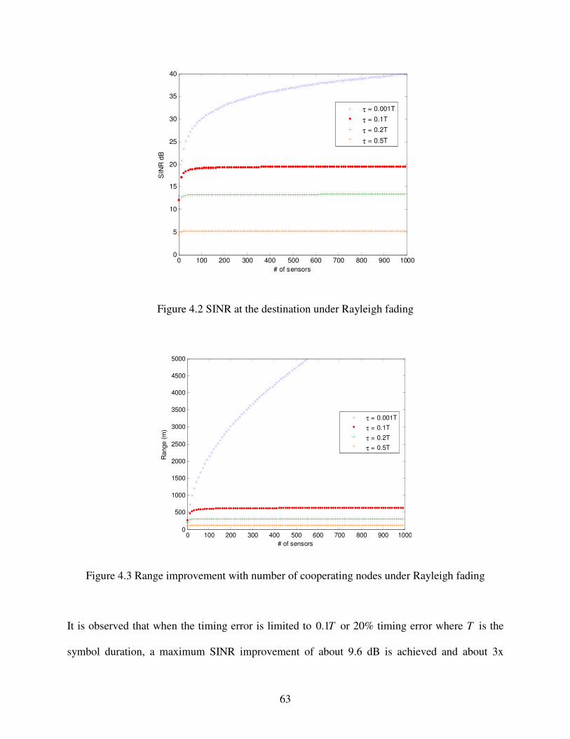
63

0 100 200 300 400 500 600 700 800 900 10000

5

10

15

20

25

30

35

40

# of sensors

SIN

R d

B

τ = 0.001T

τ = 0.1T

τ = 0.2T

τ = 0.5T

Figure 4.2 SINR at the destination under Rayleigh fading

0 100 200 300 400 500 600 700 800 900 10000

500

1000

1500

2000

2500

3000

3500

4000

4500

5000

# of sensors

Ran

ge (

m)

τ = 0.001T

τ = 0.1T

τ = 0.2T

τ = 0.5T

Figure 4.3 Range improvement with number of cooperating nodes under Rayleigh fading

It is observed that when the timing error is limited to 0.1T or 20% timing error where T is the

symbol duration, a maximum SINR improvement of about 9.6 dB is achieved and about 3x

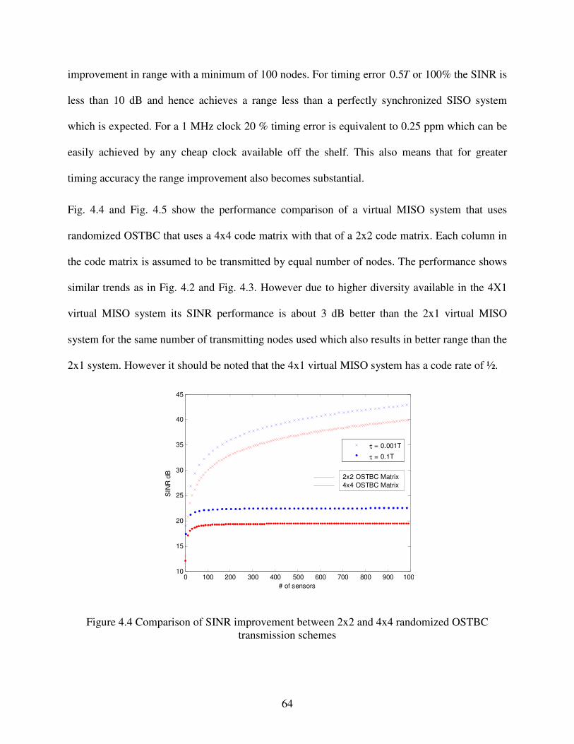
64

improvement in range with a minimum of 100 nodes. For timing error 0.5T or 100% the SINR is

less than 10 dB and hence achieves a range less than a perfectly synchronized SISO system

which is expected. For a 1 MHz clock 20 % timing error is equivalent to 0.25 ppm which can be

easily achieved by any cheap clock available off the shelf. This also means that for greater

timing accuracy the range improvement also becomes substantial.

Fig. 4.4 and Fig. 4.5 show the performance comparison of a virtual MISO system that uses

randomized OSTBC that uses a 4x4 code matrix with that of a 2x2 code matrix. Each column in

the code matrix is assumed to be transmitted by equal number of nodes. The performance shows

similar trends as in Fig. 4.2 and Fig. 4.3. However due to higher diversity available in the 4X1

virtual MISO system its SINR performance is about 3 dB better than the 2x1 virtual MISO

system for the same number of transmitting nodes used which also results in better range than the

2x1 system. However it should be noted that the 4x1 virtual MISO system has a code rate of ½.

0 100 200 300 400 500 600 700 800 900 100010

15

20

25

30

35

40

45

# of sensors

SIN

R d

B

τ = 0.001T

τ = 0.1T

2x2 OSTBC Matrix4x4 OSTBC Matrix

Figure 4.4 Comparison of SINR improvement between 2x2 and 4x4 randomized OSTBC transmission schemes

65

0 100 200 300 400 500 600 700 800 900 10000

1000

2000

3000

4000

5000

6000

7000

8000

9000

10000

# of sensors

Ran

ge (m

)τ = 0.001T

τ = 0.1T

2x2 OSTBC Matrix4x4 OSTBC Matrix

Figure 4.5 Comparison of range improvement between 2x2 and 4x4 randomized OSTBC transmission schemes

4.4 Conclusions

In this chapter we investigated the relationship between node density and range improvement in

the presence of timing error for a cooperative diversity system that uses randomized space-time

block coding. Using the analysis we have found that with timing error limits the range

improvement. The range ceases to improve appreciably beyond a certain number of nodes with

timing error. The computational results using our analysis provide the optimal number of nodes

required for cooperation under a given margin of timing error for a certain amount of range

improvement.

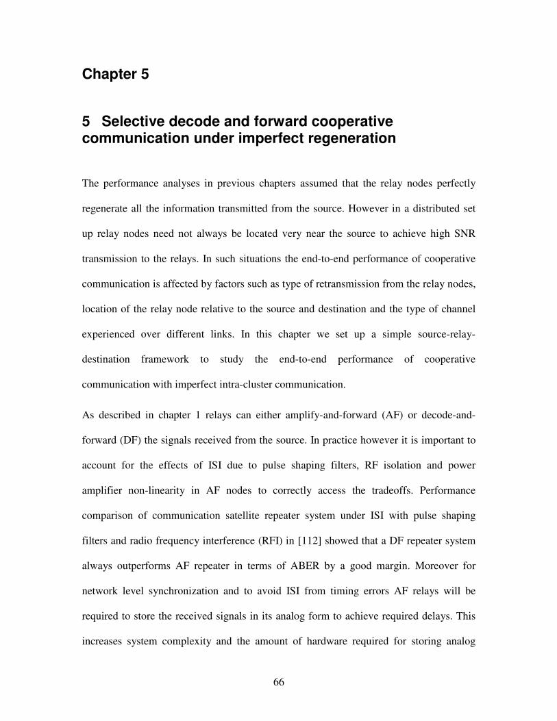
66

Chapter 5

5 Selective decode and forward cooperative communication under imperfect regeneration

The performance analyses in previous chapters assumed that the relay nodes perfectly

regenerate all the information transmitted from the source. However in a distributed set

up relay nodes need not always be located very near the source to achieve high SNR

transmission to the relays. In such situations the end-to-end performance of cooperative

communication is affected by factors such as type of retransmission from the relay nodes,

location of the relay node relative to the source and destination and the type of channel

experienced over different links. In this chapter we set up a simple source-relay-

destination framework to study the end-to-end performance of cooperative

communication with imperfect intra-cluster communication.

As described in chapter 1 relays can either amplify-and-forward (AF) or decode-and-

forward (DF) the signals received from the source. In practice however it is important to

account for the effects of ISI due to pulse shaping filters, RF isolation and power

amplifier non-linearity in AF nodes to correctly access the tradeoffs. Performance

comparison of communication satellite repeater system under ISI with pulse shaping

filters and radio frequency interference (RFI) in [112] showed that a DF repeater system

always outperforms AF repeater in terms of ABER by a good margin. Moreover for

network level synchronization and to avoid ISI from timing errors AF relays will be

required to store the received signals in its analog form to achieve required delays. This

increases system complexity and the amount of hardware required for storing analog

67

signals in an AF relay. A DF relay on the other hand relies on digital signal processing

which provides higher flexibility and performance at an additional complexity of a

decoder. This makes a DF relay based cooperative communication more practical.

From a performance perspective symbol error probability analyses of cooperative

diversity based on AF relaying have been reported in [39] and [41]. In the case of simple

DF based cooperative diversity, simulation results in [113] show that the system does not

achieve full diversity unless the links operate at very high SNRs. This limitation has been

shown to be overcome by using adaptive DF relaying strategies studied in [22], [24] and

[114]. However the above schemes require knowledge of instantaneous (per fading

realization) channel state information [24] or the instantaneous ABER [114] of each link

for required adaptation at the destination. This can be difficult to achieve for a real-time

application. It has also been shown that DF relay transmissions called coded cooperation

that make use of error correction codes and cyclic redundancy check (CRC) improve the

error performance considerably [115]. For practical implementation however a tradeoff

between error performance and excess processing will need to be determined as the

processing required for decoding and re-encoding operations can result in higher latency

and therefore reduce spectral efficiency.

In this chapter we investigate the ABER performance of a simpler (easier to implement)

selective-decode-and-forward (SDF) scheme where the relay determines when to forward

a symbol based on a preset SNR threshold. The framework presented in this work gives

insight into the combined effects of propagation, geometry and imperfect transmission

from the relay. Through our analysis we show the effect of different factors that

contribute to the end-to-end ABER performance of an SDF system and try to find

68

answers to questions like: (i) When is it beneficial for a relay to cooperate? (ii) Does

geometry affect performance? (iii) Is there an optimum SNR threshold? (iv) Is an

optimum transmit-power allocation between source and relay possible? (v) Is the SDF

scheme more energy efficient than a SISO scheme?

The chapter is organized as follows. Section 5.2 describes the system model for SDF

relay transmission. In section 5.3 we describe the end-to-end ABER analysis. Section 5.4

we derive an expression for optimum SNR threshold. In section 5.6 we discuss the

computational results based on the ABER analysis that includes study of the effects of

power allocation, propagation, relative location of the relay and energy efficiency. Next

we present the performance analysis of a novel maximum a-posteriori probability (MAP)

detector based SDF relay system in section 5.7. Finally we draw our conclusions in

section 5.8.

5.1 System model

We consider a classical relay based cooperative communication system consisting of a

source, a relay and a destination node. Communication takes place in two phases, the

broadcast and the relay phase, due to the half-duplex constraint at the relay. In broadcast

phase the source broadcasts information to both the relay and destination. Based on the

signal quality of the received signal, the relay decides whether to decode and forward the

information to the destination. The signal quality is based on a predetermined SNR

threshold level below which the relay decides not to transmit in the relay phase. If the

received SNR falls above the threshold, then the relay transmits the decoded information

to the destination. At the destination in the relay phase, the receiver combines the signal

69

received in the broadcast phase and the signal transmitted from the relay using maximal

ratio combining (MRC) based diversity combining. However in the event where the relay

remains silent in the relay phase the symbol decisions are made solely based on signal

received from the source.

Before we get into the details of the analysis it is important to mention that a more

general maximum likelihood (ML) receiver based design that achieves optimum

performance for a DF scheme was reported in [23]. Due to the complexity involved in its

implementation this scheme was further simplified to sub-optimal versions called λ -

MRC and cooperative-MRC (C-MRC) schemes in [24] and [114] respectively that

achieve full diversity at comparable performance to the ML scheme. In λ -MRC the relay

retransmits information received from the source regardless of decoding error at the relay.

At the destination, a parameter [ ]0,1λ ∈ based on knowledge of probability of error in

source-to-relay link is used to appropriately weight the relay-destination signal received

at the destination for the MRC combining process. In the case of C-MRC, it is proposed

that the instantaneous equivalent SNR of the two-hop source-relay-destination channel is

first obtained through transmission of pilot symbols which is then used to appropriately

weight the relay-destination signal received at the destination for the MRC combining

process. As pointed out earlier the requirement for instantaneous per channel information

makes the system implementation complex and hence the simple SDF scheme described

above will be investigated for performance improvements.

70

The normalized mean path SNR is given by 2 2ij ijEσ α= where ij represents the link

between thi and thj nodes and ijα is a random variable representing the fading amplitude

process. This allows for capturing the effects pathloss and distance into 2ijσ .

Most of the researches on cooperative diversity have typically looked at performance of

symmetric networks. Fig. 5.1 shows five possible scenarios keeping the source-to-

destination constant. The relative position of the relay and powers allocated for each

node can affect the relative power gains over the links affecting performance. To

understand the effect of network geometry on the performance of the system, our

parameterization which is similar to [116] is discussed as follows. We let

( )2ij SD ijd d

µσ = where SDd the distance from source to the destination and ijd is the distance

between thi and thj nodes while the pathloss coefficient is denoted by µ . Given angle θ as

seen in Fig. 5.1 one can evaluate SRd using trigonometric identity for predetermined

values of RDd . Now by letting 1SDd = one can readily determine the normalized path mean

SNRs 2SRσ and 2

RDσ . Next we describe the signals received at each node and allocation of

power.

The signal received at the relay and the destination in phase one and two can be written

as

broadcast phase

ˆ relay phase

SR S SR S SR

SD S SD S SD

RD S RD R RD

r b E n

r b E n

r b E n

αα

α

= +

= +

= +

(5.1)

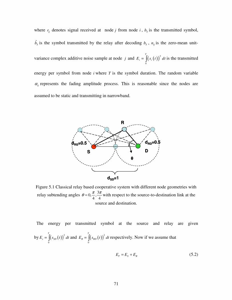
71

where ijr denotes signal received at node j from node i , Sb is the transmitted symbol,

Sb is the symbol transmitted by the relay after decoding Sb , ijn is the zero-mean unit-

variance complex additive noise sample at node j and ( )( )2

0

T

i iE s t dt= is the transmitted

energy per symbol from node i where T is the symbol duration. The random variable

ijα represents the fading amplitude process. This is reasonable since the nodes are

assumed to be static and transmitting in narrowband.

S D

R

dSD=1

dRD=0.5dRS=0.5

S D

R

dSD=1

dRD=0.5dRS=0.5

Figure 5.1 Classical relay based cooperative system with different node geometries with

relay subtending angles 30, ,

4 4π πθ = with respect to the source-to-destination link at the

source and destination.

The energy per transmitted symbol at the source and relay are given

by ( )( )2

0

T

s SDE s t dt= and ( )( )2

0

T

R RDE s t dt= respectively. Now if we assume that

T S RE E E= + (5.2)

72

Then we can write ( ) and 1S T R TE E E Eδ δ= = − . The average received SNR for the source-

to-destination link and the source-to-relay link can be written as 2

22T SD

SDSD

Eδ σγη

= and

2

22T SR

SRSR

Eδ σγη

= respectively. In the case of relay-to-destination link, for the duration when

relay transmission occurs, the average received SNR is given by ( ) 2

2

1

2T RD

RDRD

Eδ σγ

η−

= . The

two-sided power spectral density of AWGN used in the above expressions is 2 0

2ij

Nη = .

The bit error probability of the selective decode-and-forward scheme with BPSK

modulation is primarily influenced by three mutually exclusive events which is given by

( ) ( ) ( )1SR SR SR

DIV XSD SR SRe e e ee e

P P F P P P Pγ γ γ γ γ∗ ∗> >= ⋅ + − ⋅ + ⋅ (5.3)

The first term on the RHS of equation (5.3) represents the event where the signal quality

from source-to-relay, SRγ is below the specified SNR threshold level denoted

byγ ∗ represented by the CDF ( )PrSR SRFγ γ γ ∗= < . Thus in this case the relay remains silent

in phase-2 and the detection at the destination is solely based on probability of symbol

error in source-to-destination link represented by SDeP . The second and third terms

represent the event where the signal quality of the source-to-relay link is above the SNR

threshold SRγ γ ∗> and the relay decodes and decides to transmit in phase two. The second

term represents the case where the relay correctly decoded the symbol transmitted from

the source in phase one with probability ( )1SR

SR

eP

λ γ ∗>− and in phase two after coherent

diversity combining of the two received signals at the destination the transmitted symbol

73

is decoded in error with probability ( )DIVeP . The third term represents the case where the

relay in phase one decodes the symbol transmitted from the source in error SReP even

though SRγ γ ∗> . This can happen due to improper choice of threshold level. This leads to

wrongful combining at the destination in phase two where ( )XeP denotes the probability of

error due to wrongful combining. In [116], the results are based on the assumption

that ( ) 0.5XeP ≤ . However, the value of ( )X

eP depends on the power of the signal received at

the destination from the relay which can vary depending on the location of the relay. As

will be shown later in section 5.4 the effect of ( )XeP on the end-to-end ABER can be

minimal when the relay is near the source and can be a dominant factor when it is near

the destination. Hence in this work we derive a numerical expression that evaluates the

exact value of ( )XeP for BPSK and an upper bound for MPSK system to facilitate

computation of an exact end-to-end ABER performance of the SDF system.

The symbol error probability (SEP) for an arbitrary two dimensional signal constellation

can be expressed in a desirable exponential form. For example in the M-PSK case the

SEP is given by [90] as

( ) ( )( )

( )1 2

20

sin1exp

sin

M M

e

MP d

π γ πγ θ

π θ

− −=

(5.4)

The probability of error SR

SR

eP

γ γ ∗> in (5.3) can now be computed as

( ) ( ) ( )( )

( )1 2

20

sin1,

sinSRSR

M MSR

ee

MP P f d d

π

γ γγ γγ

πγ γ γ φ γ θ

π θ∗

∗

−∞∗

>

= =

(5.5)

74

where ( ),s yγφ is the marginal MGF which is known in closed-form for Rayleigh, Rice,

Nakagami-m and Nakagami-q channel models [117, eq. B.1 - B.5] . For the special case

of ( ) ( ),0s sγ γφ φ= which is the MGF of γ , readily available in closed-form for the

distributions mentioned above, the expression in the right hand side of (5.5) can be used

to compute SDeP in (5.3).

Now we evaluate ( )DIVeP . The signals are assumed to be combined at the receiver using

MRC diversity combining scheme. Therefore the decision statistic after matched filtering

and MRC combining is given by

( )

( ) 2 2 2 2ˆ 1

1

SD SD RD RD T SD SD T RD RD

T SD SD SD T RD RD RD

Z r r E E

E n E n

α α δ σ α δ σ α

δ σ α δ σ α

∗ ∗

∗ ∗

= ℜ + = + −

+ ℜ + − (5.6)

The effective SNR at the output of the diversity combiner in (5.6) can now be written as

( )( )( )( )

2 22 2 2 2

2 2 2 2

1

1SD SD RD RD T

DIV SD RDSD SD RD RD T

E

E

δσ α δ σ αγ γ γ

δσ α δ σ α+ −

= = ++ −

(5.7)

Assuming that the symbols transmitted by the source is retransmitted correctly by the

relay the bit error probability at the output of the diversity combiner at the destination can

be calculated for any two-dimensional arbitrary modulation using MGF based methods

[85]. For M-PSK the MGF ( ) ( ) ( )DIV SD RD

t t tγ γ γφ φ φ= ⋅ where SDγ and RDγ are independent

and the individual MGFs are readily available for Rayleigh, Rice and Nakagami

distributions [85]. Hence ( )DIVeP can be expressed as

( ) ( )( )

( ) ( )( )

1 2 2

2 20

sin sin1sin sinSD RD

M MDIV

e

M MP d

π

γ γπ π

φ φ θπ θ θ

− =

(5.8)

75

To compute ( )XeP we visit equation (5.6). In this case the first term on the RHS is the

desired signal and the second term results from a symbol that is decoded incorrectly and

transmitted by the relay. In the following we derive an exact expression for ( )XeP for

BPSK modulation. It is difficult to derive the exact expression for ( )XeP under MPSK

modulation and hence a tight upper bound is derived for general constellation.

The desired portion of the received signal in (5.6) for the case of wrongful combining

with BPSK can be written as

( )2 2 2 21T SD SD T RD RDY E Eδ σ α δ σ α= − − (5.9)

The variance due to noise in (5.6) is given by

( )( )2 2 2 2 2 012T SD SD RD RD

NE n E δσ α δ σ α= + − (5.10)

Now ( )XeP can be obtained for a BPSK system as

( ) ( ) ( ) 1 2ˆPr 0 1 PrX

e sP Z b n Y P P= > = − = > = + (5.11)

where

( )( ) ( )

( ) ( )

2 2 2 21 2 2 2 2

00 1

2 11

1

RD

SD RD

TSD SD RD RD

SD SD RD RD

SD RD SD RD

EP Q

N

f f d d

δαδ

α α

δσ α δ σ αδσ α δ σ α

α α α α

∞ ∞

−

= − −

+ −

×

(5.12)

and

( )( ) ( )( ) ( )

1

2 2 2 22 2 2 2 2

00 0

2 11 1

1

RD

SD RD

TRD RD SD SD

SD SD RD RD

SD RD SD RD

EP Q

N

f f d d

δαδ

α α

δ σ α δσ αδσ α δ σ α

α α α α

−∞

= − − − + −

×

(5.13)

76

In the case of an MPSK constellation with M>2, an upper bound for ( )XeP can be found as

follows. Examining (5.6), for an MPSK symbol transmitted by the source the worst case

scenario for wrongful combining happens when the relay transmits a symbol that lies

diametrically opposite to it in the constellation. Hence when a reference symbol with

phase equal to zero in the MPSK constellation is transmitted from the source the decision

statistic after MRC combing for the worst case can be written as

( ) ( ) 2 2 2 2ˆ 1 1T SD SD T RD RD T SD SD SD T RD RD RDZ E E E n E nδ σ α δ σ α δ σ α δ σ α∗ ∗= − − + ℜ + − (5.14)

The effective received SNR for this case can be written as

( )( )

( )( )

22 2 2 2 2

2 2 2 2 0

1

12

T SD SD RD RDeff

T SD SD RD RD

E

NE

δσ α δ σ αγ

δσ α δ σ α

− −=

+ − (5.15)

A tight upper bound for symbol error probability can be computed as ( )1 2

XeP P P= + where

( ) ( ) ( )

( )2

1

1 20 01

sin1

expsin SD RD

RD

M M

eff SD RD SD RDMP f f d d d

π

α αδα

δ

π

γ α α θ α απ θ

−∞ ∞

−

= −

(5.16)

and

( ) ( ) ( )( )

1 21

2 20 0 0

sin1

1 expsin

RD

SD RD

M M

eff SD RD SD RDMP f f d d d

δα πδ

α α

π

γ α α θ α απ θ

−−∞

= − −

(5.17)

A looser upper bound for ( )XeP can also be found by invoking the union bound for an

MPSK constellation where the minimum distance is given by ( )min sind Mπ= . Now if

77

average desired symbol energy to noise ratio ( )2min

0 0

symE d

N N= then the average symbol

energy transmitted by the relay which is diametrically opposite in the MPSK

constellation is given by

( )( )

22_ max min

0 min 0 0

2 sin

sinRD sym sym symE E EMd dN d N M N

ππ

− −= =

(5.18)

Now from (5.14) the probability of error from union bound after wrongful combining can

be written as

( )( )

( )

2 2 2 2max min

min

2 2 2 2max min 0

min

12

12

T SD SD RD RDX

e AWGN

T SD SD RD RD

d dE

dP Q

d d NE

d

δσ α δ σ α

δσ α δ σ α

− − − =

− + −

(5.19)

Now ( )XeP for MPSK under fading can be determined as

( ) ( ) ( ) ( ) 0 0

SD RD

X Xe e AWGN SD RD SD RDP P f f d dα αα α α α

∞ ∞

= (5.20)

Next we derive the optimum SNR threshold at the relay that minimizes ABER

performance.

5.2 Optimum SNR threshold γ ∗ From (5.3) it can be observed that the ABER, eP , can be optimized i with respect to the

SNR threshold γ ∗ for a fixed fractional power allocation δ and a given geometry.

Optimum γ ∗ is obtained by minimizing the ABER. This is achieved by taking the

derivative of eP over γ ∗ and then setting the result to zero i.e. 0edP dγ ∗ = . By noting that

78

( ) ( )0

SR SRF f x dx

γ

γ γγ∗

∗ = and that ( ) ( )b

a

df x f a

da= − and ( ) ( )

b

a

df x f b

db= we can write the

derivative of eP as

( ) ( ) ( ) ( ) ( ) ( ) ( )

( ) ( ) ( ) ( )( ), ,

,

SR SR SR

SR

DIV XSDee e e AWGN e e AWGN

DIV XSDe e AWGN e e

dPP f P P f P P f

d

f P P P P

γ γ γ

γ

γ γ γ γ γγ

γ γ

∗ ∗ ∗ ∗ ∗∗

∗ ∗

= − − + −

= + −

(5.21)

Equating (5.21) to zero and observing that ( ) 0SR

fγ γ ∗ ≥ the optimum SNR threshold is

obtained when either 0γ ∗ = or when ( ) ( ) ( ),

SDe

e AWGN X DIVe e

PP

P Pγ ∗ =

−. For BPSK

case, ( ) ( ), 0.5e AWGNP erfcγ γ∗ ∗= and therefore

( ) ( )

2

1 2 SDe

opt X DIVe e

Perfc

P Pγ ∗ −

= −

(5.22)

Notice that the optimum SNR threshold 0optγ ∗ = unless ( ) ( )0 1SD

eX DIV

e e

P

P P< <

−. It is also

interesting to note that the optimal threshold does not directly depend on the quality of

source-to relay channel. In practice however ( )XeP cannot be determined. However, since

( ) 1XeP < and in most cases ( ) ( )X DIV

e eP P>> , the optimum value of SNR threshold can be

approximated as ( ) 21 2 SD

opt eerfc Pγ ∗ − = .

In the next section we discuss the computation and comparison of energy efficiency of

SDF scheme with a SISO scheme.

79

5.3 Energy efficiency of SDF based cooperative communication Ad-hoc wireless networks such as sensor networks usually operate under energy limited

conditions and therefore energy efficiency is an important design metric for improving

the life time of a network [5].

Very few papers in the past have investigated energy efficiency issues of different

cooperative communication schemes. In [118] the authors presented an energy efficiency

analysis for different relay strategies based on a method established in [119] for

bandwidth-power tradeoff analysis under low-power low-spectral-efficiency regime. It is

shown that under information-theoretic limits decode and forward cooperative relaying

provides substantial improvement in energy efficiency compared to a SISO transmission.

In a more direct approach [34] and [120] considered a cooperative MIMO system where

the energy consumed is computed as the sum of the individual transmission energies. The

individual transmission energies include (i) transmit-energy required for the local (short

distance) communication between source and the relay links, (ii) the cooperative MIMO

transmit-energy required for long haul between relay nodes and the destination and (iii)

the circuit energy consumed at each node. The cooperative MIMO transmit-energy in (ii)

is found by converting the relay-destination links into an equivalent point-to-point MIMO

model. In [121] energy efficiency of a decode-and-forward protocol that exploits macro-

diversity was analyzed by reducing the system to an equivalent rake receiver model.

Energy efficiency in the case of cooperative beamforming with a simple relay selection

criterion is investigated in [122].

In the analyses of the works reported above with the exception of [122] it is commonly

assumed that the relay nodes perfectly regenerate the information transmitted from the

80

source even though the source-to-relay links may be operating at a predefined bit error

probability (BEP). This helps in breaking down the end-to-end analysis into two parts; a

broadcast system for source-to-relay communication and an equivalent MIMO [34], rake

receiver [121] or a beamforming system [122] for relay-to-destination communication.

No cost has been associated with the extra energy that may be required for perfect

regeneration for a given BEP at the relay. Perfect regeneration at a given BEP requires

either the use of forward error correction (FEC) or use of cyclic redundancy check (CRC)

at the MAC layer to make sure that the packet received from the source has no errors. To

perform an accurate and fair evaluation for energy efficiency in the above cases it is

important to accommodate excess energy consumed in transmitting redundant bits when

FEC is used or to calculate the excess energy consumed in the average number of

retransmissions when CRC is considered.

In the analysis of energy efficiency for the SDF scheme considered in this chapter we

circumvent the above problem by making use of the exact end-to-end average bit error

rate (ABER) that accounts for the imperfect regeneration at the relays. This helps in

obtaining more realistic comparison of SDF scheme against a SISO system. In the

following we discuss the methodology used to find the energy consumed by the SDF

scheme.

Let the average power consumed in a SISO transmission between source and destination

be given by

_ _SISO Tx Tx ckt Rx cktP P P P= + + (5.23)

81

where TxP is the transmit power associated with the power amplifier, _Tx cktP is the power

consumed by the analog and RF circuitry during transmission and _Rx cktP is the energy

consumed during reception at the destination. The circuit energies become important in

applications that operate under low power for example, sensor networks.

The total average power consumed by the source and relay nodes for the selective decode

and forward scheme discussed in section II can be written as

( ) ( ) ( )_ _ _1 2 3SR SR SRSDF avg S R Tx ckt Rx cktP P F P F P F Pγ γ γ= + − + − + − (5.24)

where SP and RP are the transmit powers of the source and relay nodes respectively. A

factor of 0.5 associated to the circuit power is due to the fact that the source and the

nodes are active only for half the duration compared to SISO transmission. The

relationship with transmitted energy per bit is given by S SE P T= and R RE P T= . It should

be noted that the rate at which data is transmitted in the selective decode and forward

(SDF) system is half that of the SISO system. This is because the source in the case of

SDF system only transmits for half the total duration of transmission of a SISO system.

Hence if SISOR is the bit rate of the SISO system the bit rate of the selective decode and

forward system is given by 2SDF SISOR R= .

The average transmission powers TxP , SP and RP are computed as follows. In the case of

SISO system, we consider the source-to-destination link discussed in section II and

compute the average bit error rate (ABER) for different values of0

TxEN

. For a given noise

level one can compute TxE which is the average transmission energy (Joules) per bit and

calculate the transmitted power as Tx Tx SISOP E R= . Next in the case of SDF transmission,

82

we assume that the total transmission power when both the source and the relay transmit

equals the transmission power in the SISO case such that Tx S RP P P= + . However, from

(5.24) it can be observed that the average power transmitted in the SDF scheme will

always be less than TxP . Using (5.3) we can now calculate the ABER for different values

of 0

TEN

and also for different values of power allocationδ where TE is given by (5.2). The

value of TE can be determined for a given noise level and hence corresponding

transmission power values can be calculated as S T SISOP E Rδ= and ( )1R T SISOP E Rδ= − . These

values can now be substituted in (5.23) and (5.24) to compute the average power

consumed under each scheme. It should be noted that we have assumed that all the nodes

are able to transmit with the same bandwidth.

To compare the energy efficiencies we need to compute the energy consumed per bit for

a given BEP at the destination. The energy consumed per bit can be calculated as the

ratio of the total average power consumed (explained above) to the bit rate associated

with the system given by SISO

SISO

PR

and _ _2SDF avg SDF avg

SDF SISO

P P

R R= for SISO and SDF systems

respectively.

In the following section we discuss the computational results from the analysis and

comment on the observations made.

5.4 Computational results and remarks In this section we first present the numerical results from the framework developed for

analysis of cooperative relay system in section 5.1 and discuss the related performance

issues. This is followed by computational results on energy consumption of the SDF

83

system as discussed in section 5.3 and a discussion on the significance of the results with

respect to energy efficiency in a sensor network.

5.4.1 ABER performance Fig. 5.2 shows the ABER performance comparison between numerical results from

analysis and Monte Carlo simulation for a BPSK system where all the links experience

Rayleigh fading. The analytical results are in very good match with simulation and hence

validate our analysis. It is also generally observed that the relay in transmit-cluster

outperforms relay in receive-cluster. The ABER performance at higher SNR threshold

(10 dB) is better than lower SNR threshold (-10 dB) for higher 0TE N and vice-versa for

lower values of 0TE N . These observations will be more clearly explained in the

following discussion.

0 5 10 15 20 25 3010

-6

10-5

10-4

10-3

10-2

10-1

100

ET/N0 (dB)

AB

ER

γ* = 10dB, Rx Cluster θ = π/4

γ* = 10dB, Tx Cluster θ = π/4

γ* = -10dB, Rx Cluster θ = π/4

γ* = -10dB, Tx Cluster θ = π/4

Monte Carlo Simulation

Figure 5.2 Validation of ABER performance from Numerical analysis and Monte Carlo

Simulation of SDF cooperative communication system BPSK modulation.

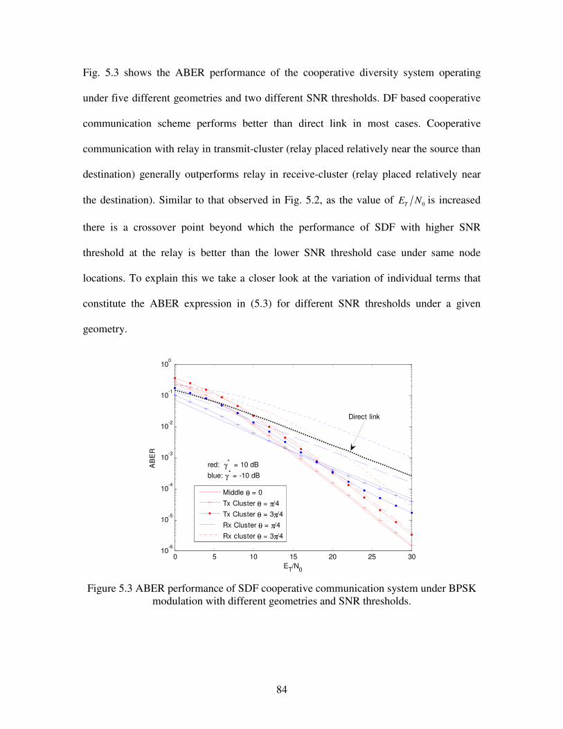
84

Fig. 5.3 shows the ABER performance of the cooperative diversity system operating

under five different geometries and two different SNR thresholds. DF based cooperative

communication scheme performs better than direct link in most cases. Cooperative

communication with relay in transmit-cluster (relay placed relatively near the source than

destination) generally outperforms relay in receive-cluster (relay placed relatively near

the destination). Similar to that observed in Fig. 5.2, as the value of 0TE N is increased

there is a crossover point beyond which the performance of SDF with higher SNR

threshold at the relay is better than the lower SNR threshold case under same node

locations. To explain this we take a closer look at the variation of individual terms that

constitute the ABER expression in (5.3) for different SNR thresholds under a given

geometry.

0 5 10 15 20 25 3010

-6

10-5

10-4

10-3

10-2

10-1

100

ET/N0

AB

ER

Middle θ = 0Tx Cluster θ = π/4Tx Cluster θ = 3π/4Rx Cluster θ = π/4Rx cluster θ = 3π/4

Direct link

red: γ* = 10 dBblue: γ* = -10 dB

Figure 5.3 ABER performance of SDF cooperative communication system under BPSK

modulation with different geometries and SNR thresholds.

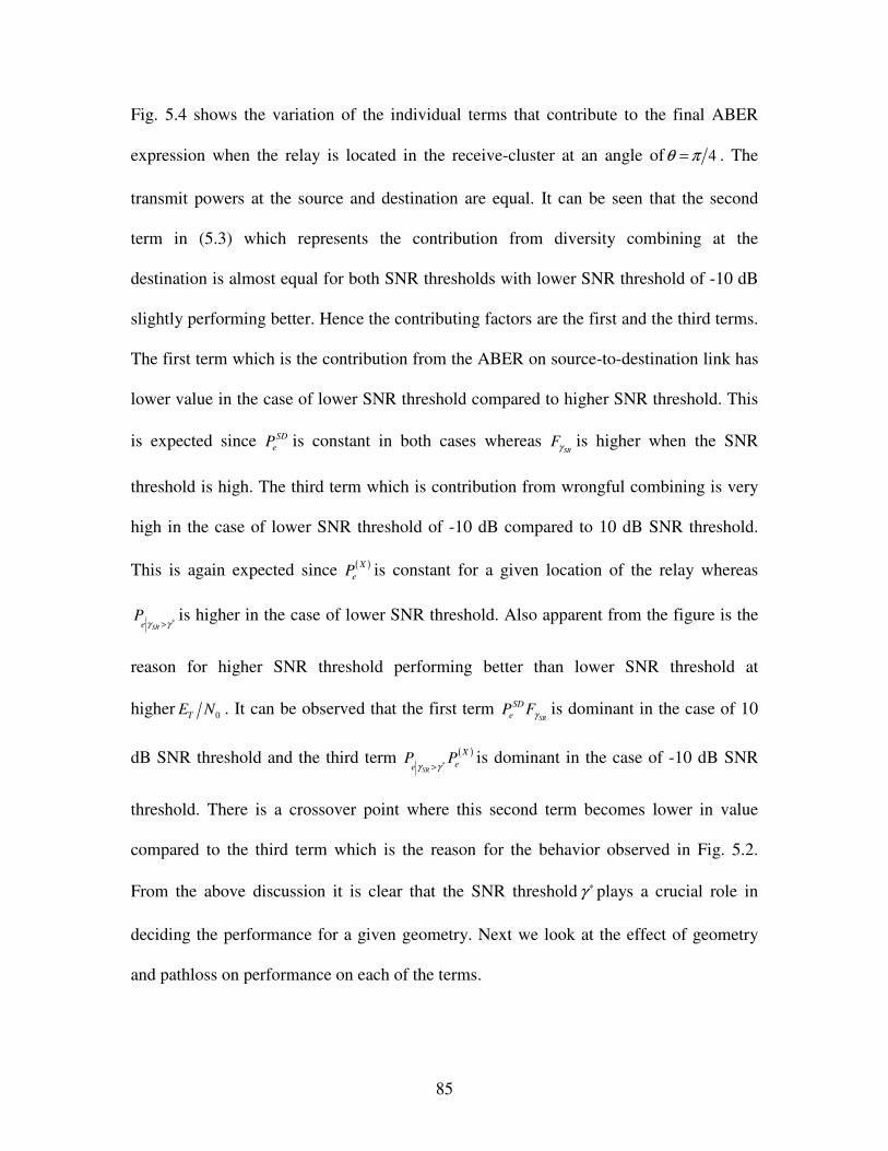
85

Fig. 5.4 shows the variation of the individual terms that contribute to the final ABER

expression when the relay is located in the receive-cluster at an angle of 4θ π= . The

transmit powers at the source and destination are equal. It can be seen that the second

term in (5.3) which represents the contribution from diversity combining at the

destination is almost equal for both SNR thresholds with lower SNR threshold of -10 dB

slightly performing better. Hence the contributing factors are the first and the third terms.

The first term which is the contribution from the ABER on source-to-destination link has

lower value in the case of lower SNR threshold compared to higher SNR threshold. This

is expected since SDeP is constant in both cases whereas

SRFγ is higher when the SNR

threshold is high. The third term which is contribution from wrongful combining is very

high in the case of lower SNR threshold of -10 dB compared to 10 dB SNR threshold.

This is again expected since ( )XeP is constant for a given location of the relay whereas

SReP

γ γ ∗>is higher in the case of lower SNR threshold. Also apparent from the figure is the

reason for higher SNR threshold performing better than lower SNR threshold at

higher 0TE N . It can be observed that the first term SR

SDeP Fγ is dominant in the case of 10

dB SNR threshold and the third term ( )SR

Xee

P Pγ γ ∗>

is dominant in the case of -10 dB SNR

threshold. There is a crossover point where this second term becomes lower in value

compared to the third term which is the reason for the behavior observed in Fig. 5.2.

From the above discussion it is clear that the SNR threshold γ ∗ plays a crucial role in

deciding the performance for a given geometry. Next we look at the effect of geometry

and pathloss on performance on each of the terms.

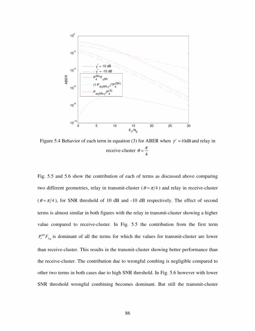
86

0 5 10 15 20 25 3010

-10

10-8

10-6

10-4

10-2

100

ET/N0

AB

ER Pe

SD*FγSR

(1-Pe|γSR>γ*)*Pe(DIV)

Pe|γSR>γ*Pe(X)

γ* = 10 dB

γ* = -10 dB

Figure 5.4 Behavior of each term in equation (3) for ABER when 10dBγ ∗ = and relay in

receive-cluster 4πθ =

Fig. 5.5 and 5.6 show the contribution of each of terms as discussed above comparing

two different geometries, relay in transmit-cluster ( 4θ π= ) and relay in receive-cluster

( 4θ π= ), for SNR threshold of 10 dB and -10 dB respectively. The effect of second

terms is almost similar in both figures with the relay in transmit-cluster showing a higher

value compared to receive-cluster. In Fig. 5.5 the contribution from the first term

SR

SDeP Fγ is dominant of all the terms for which the values for transmit-cluster are lower

than receive-cluster. This results in the transmit-cluster showing better performance than

the receive-cluster. The contribution due to wrongful combing is negligible compared to

other two terms in both cases due to high SNR threshold. In Fig. 5.6 however with lower

SNR threshold wrongful combining becomes dominant. But still the transmit-cluster

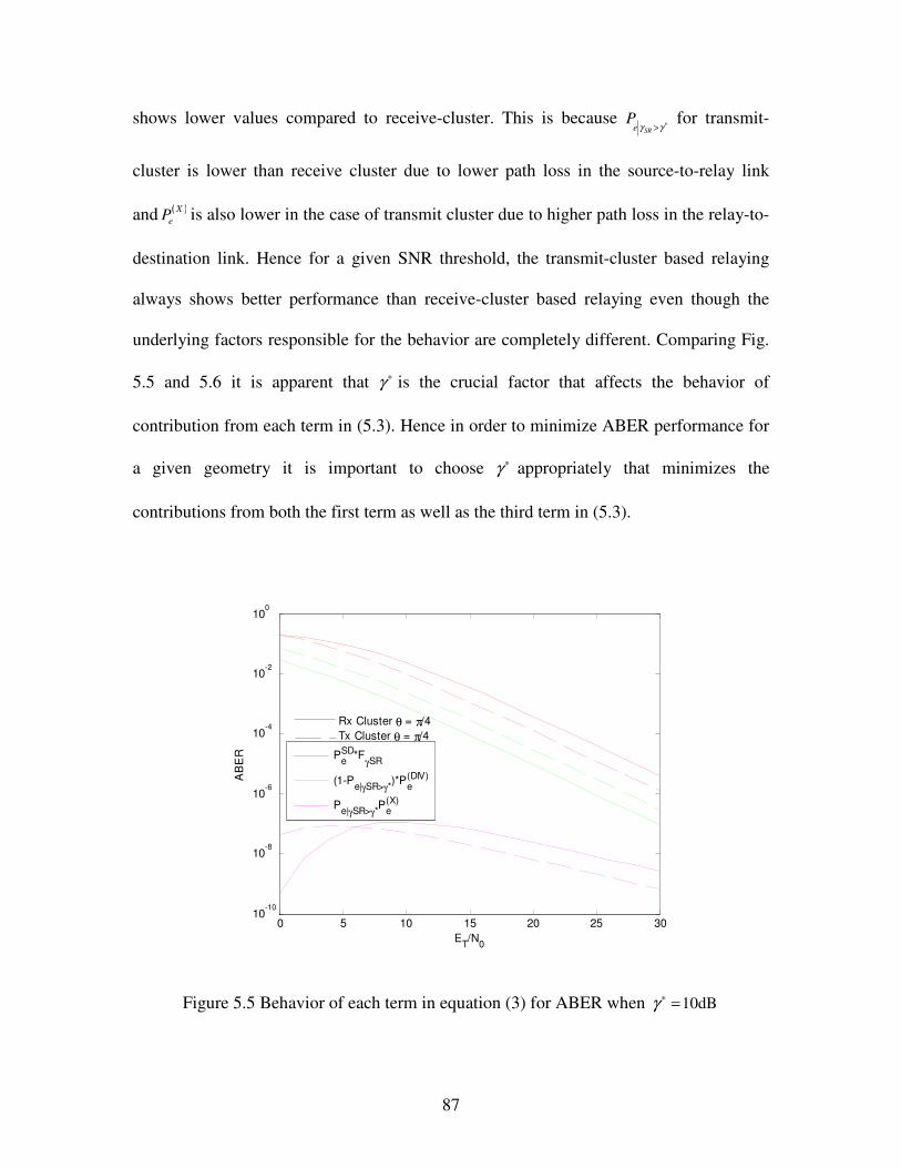
87

shows lower values compared to receive-cluster. This is because SRe

Pγ γ ∗>

for transmit-

cluster is lower than receive cluster due to lower path loss in the source-to-relay link

and ( )XeP is also lower in the case of transmit cluster due to higher path loss in the relay-to-

destination link. Hence for a given SNR threshold, the transmit-cluster based relaying

always shows better performance than receive-cluster based relaying even though the

underlying factors responsible for the behavior are completely different. Comparing Fig.

5.5 and 5.6 it is apparent that γ ∗ is the crucial factor that affects the behavior of

contribution from each term in (5.3). Hence in order to minimize ABER performance for

a given geometry it is important to choose γ ∗ appropriately that minimizes the

contributions from both the first term as well as the third term in (5.3).

0 5 10 15 20 25 3010

-10

10-8

10-6

10-4

10-2

100

ET/N0

AB

ER Pe

SD*FγSR


Pe|γSR>γ*Pe(X)

Rx Cluster θ = π/4Tx Cluster θ = π/4

Figure 5.5 Behavior of each term in equation (3) for ABER when 10dBγ ∗ =

88

0 5 10 15 20 25 3010

-8

10-7

10-6

10-5

10-4

10-3

10-2

10-1

ET/N0

AB

ER

PeSD*FγSR


Pe|γSR>γ*Pe(X)

Rx Cluster θ = π/4Tx Cluster θ = π/4

Figure 5.6 Behavior of each term in equation (3) for ABER when 10dBγ ∗ = −

Next we look at the ABER performance when both SNR threshold and power allocated is

varied while keeping the transmitted 0TE N constant. Fig. 5.7 and Fig. 5.8 show the

contour plots for ABER performance with relay in the receive-cluster ( 4θ π= ) and

transmit-cluster ( 3 4θ π= ) respectively for different values of SNR threshold and

fractional power allocated at the source nodeδ , where the total transmit SNR is fixed

at 0 15dBTE N = . In both figures there is a distinct region of values of γ ∗ and δ that result

in minimum ABER. For example in Fig. 5.7, choosing γ ∗ between 1-4dB and δ between

0.8-0.92 results in best ABER performance. This is interesting because choosing a

highest possible γ ∗ not only minimizes ABER but also improves the rate in terms of

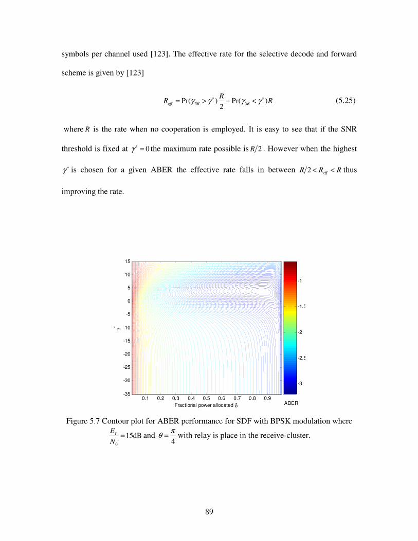
89

symbols per channel used [123]. The effective rate for the selective decode and forward

scheme is given by [123]

Pr( ) Pr( )2eff SR SR

RR Rγ γ γ γ∗ ∗= > + < (5.25)

where R is the rate when no cooperation is employed. It is easy to see that if the SNR

threshold is fixed at 0γ ∗ = the maximum rate possible is 2R . However when the highest

γ ∗ is chosen for a given ABER the effective rate falls in between 2 effR R R< < thus

improving the rate.

Fractional power allocated δ

γ*

0.1 0.2 0.3 0.4 0.5 0.6 0.7 0.8 0.9-35

-30

-25

-20

-15

-10

-5

0

5

10

15

-3

-2.5

-2

-1.5

-1

ABER

Figure 5.7 Contour plot for ABER performance for SDF with BPSK modulation where

0

15dBTEN

= and 4πθ = with relay is place in the receive-cluster.

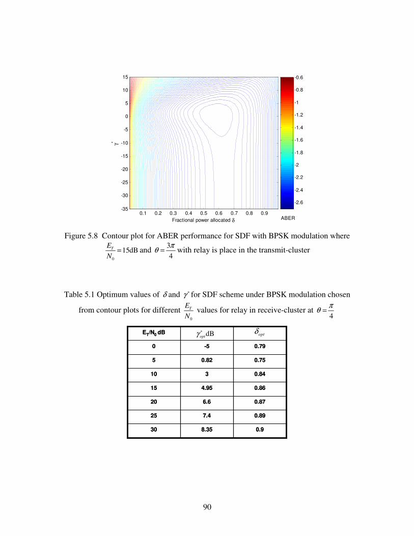
90

γ*

Fractional power allocated δ0.1 0.2 0.3 0.4 0.5 0.6 0.7 0.8 0.9

-35

-30

-25

-20

-15

-10

-5

0

5

10

15

-2.6

-2.4

-2.2

-2

-1.8

-1.6

-1.4

-1.2

-1

-0.8

-0.6

ABER

Figure 5.8 Contour plot for ABER performance for SDF with BPSK modulation where

0

15dBTEN

= and 34πθ = with relay is place in the transmit-cluster

Table 5.1 Optimum values of δ and γ ∗ for SDF scheme under BPSK modulation chosen

from contour plots for different 0

TEN

values for relay in receive-cluster at 4πθ =

0.98.3530

0.897.425

0.876.620

0.864.9515

0.84310

0.750.825

0.79-50

ET/N0 dB

0.98.3530

0.897.425

0.876.620

0.864.9515

0.84310

0.750.825

0.79-50

ET/N0 dB dBoptγ ∗optδ

91

Table 5.2 Optimum values of δ and γ ∗ for SDF scheme under BPSK modulation chosen

from contour plots for different 0

TEN

values with relay at 34πθ =

0.618.7230

0.67.8525

0.596.620

0.5954.815

0.63210

0.75-3.155

0.96-9.150

ET/N0 dB

0.618.7230

0.67.8525

0.596.620

0.5954.815

0.63210

0.75-3.155

0.96-9.150

ET/N0 dB dBoptγ ∗optδ

Next we look at the ABER performance comparison under optimum SNR threshold and

optimal power allocation which are determined from the contour plots for predefined

values of 0TE N . Highest possible value for γ ∗ is chosen from the region that minimizes

ABER on the contour plot. These values are tabulated in Table 5.1 and 5.2 for receive-

cluster ( 4θ π= ) and transmit-cluster ( 3 4θ π= ) respectively. Fig. 5.9 shows the

comparison with the case when the source and the relay transmit with equal power for

which 0.5δ = and when 0γ ∗ = . It can be observed that choosing the optimum values

always gives much better performance even when compared to the results in Fig. 5.3 and

the relative gain with optimum choice of parameters is more evident in the case where the

relay is in the receive-cluster.

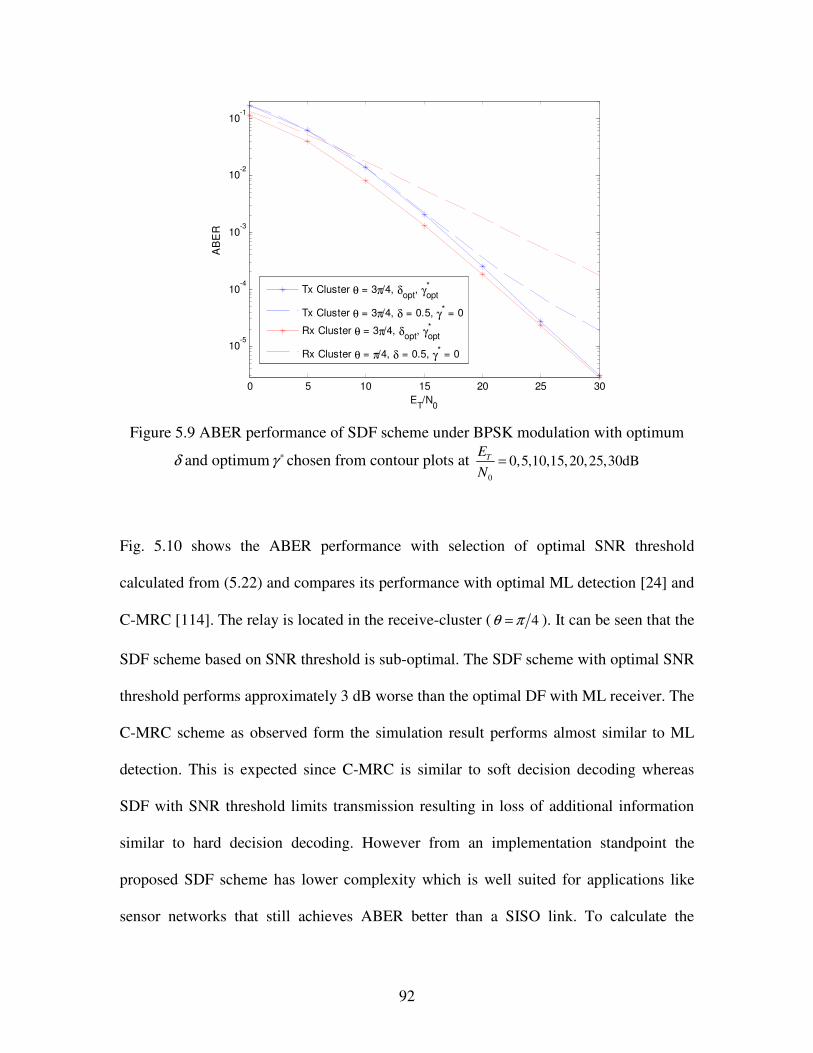
92

0 5 10 15 20 25 30

10-5

10-4

10-3

10-2

10-1

ET/N0

AB

ER

Tx Cluster θ = 3π/4, δopt, γ*opt

Tx Cluster θ = 3π/4, δ = 0.5, γ* = 0

Rx Cluster θ = 3π/4, δopt, γ*opt

Rx Cluster θ = π/4, δ = 0.5, γ* = 0

Figure 5.9 ABER performance of SDF scheme under BPSK modulation with optimum

δ and optimumγ ∗ chosen from contour plots at 0

0,5,10,15,20,25,30dBTEN

=

Fig. 5.10 shows the ABER performance with selection of optimal SNR threshold

calculated from (5.22) and compares its performance with optimal ML detection [24] and

C-MRC [114]. The relay is located in the receive-cluster ( 4θ π= ). It can be seen that the

SDF scheme based on SNR threshold is sub-optimal. The SDF scheme with optimal SNR

threshold performs approximately 3 dB worse than the optimal DF with ML receiver. The

C-MRC scheme as observed form the simulation result performs almost similar to ML

detection. This is expected since C-MRC is similar to soft decision decoding whereas

SDF with SNR threshold limits transmission resulting in loss of additional information

similar to hard decision decoding. However from an implementation standpoint the

proposed SDF scheme has lower complexity which is well suited for applications like

sensor networks that still achieves ABER better than a SISO link. To calculate the

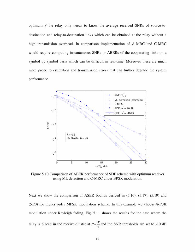
93

optimum γ ∗ the relay only needs to know the average received SNRs of source-to-

destination and relay-to-destination links which can be obtained at the relay without a

high transmission overhead. In comparison implementation of λ -MRC and C-MRC

would require computing instantaneous SNRs or ABERs of the cooperating links on a

symbol by symbol basis which can be difficult in real-time. Moreover these are much

more prone to estimation and transmission errors that can further degrade the system

performance.

0 5 10 15 20 25 30

10-5

10-4

10-3

10-2

10-1

ET/N0 (dB)

AB

ER

SDF, γ*opt

ML detection (optimum)C-MRC

SDF, γ* = 10dB

SDF, γ* = -10dB

δ = 0.5Rx Cluster θ = π/4

Figure 5.10 Comparison of ABER performance of SDF scheme with optimum receiver

using ML detection and C-MRC under BPSK modulation.

Next we show the comparison of ASER bounds derived in (5.16), (5.17), (5.19) and

(5.20) for higher order MPSK modulation scheme. In this example we choose 8-PSK

modulation under Rayleigh fading. Fig. 5.11 shows the results for the case where the

relay is placed in the receive-cluster at 4πθ = and the SNR thresholds are set to -10 dB

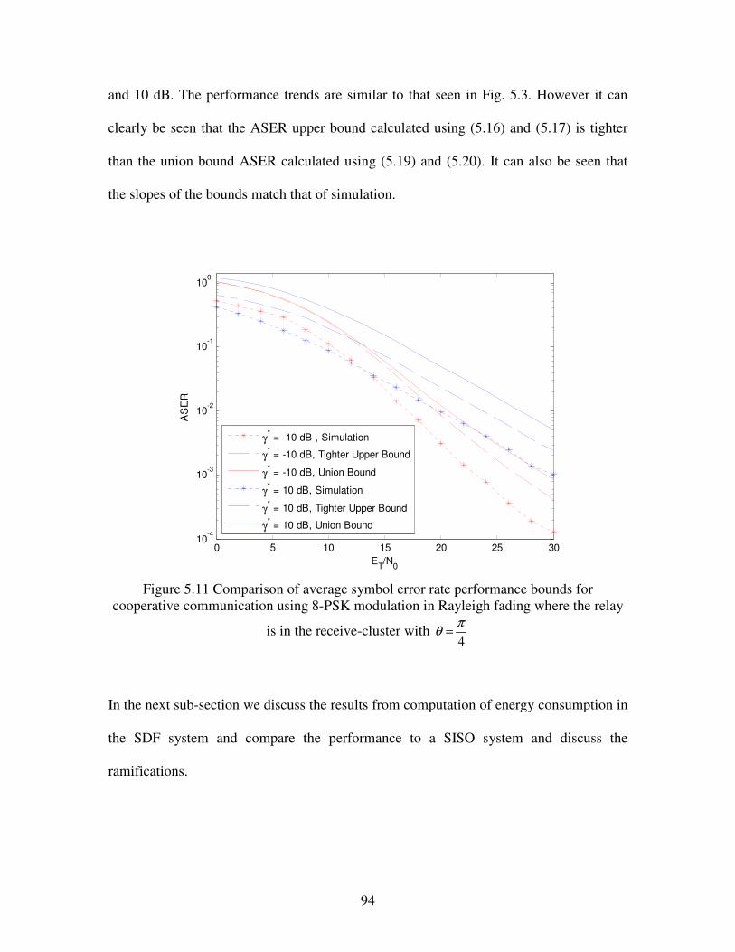
94

and 10 dB. The performance trends are similar to that seen in Fig. 5.3. However it can

clearly be seen that the ASER upper bound calculated using (5.16) and (5.17) is tighter

than the union bound ASER calculated using (5.19) and (5.20). It can also be seen that

the slopes of the bounds match that of simulation.

0 5 10 15 20 25 3010

-4

10-3

10-2

10-1

100

ET/N0

AS

ER

γ* = -10 dB , Simulation

γ* = -10 dB, Tighter Upper Bound

γ* = -10 dB, Union Bound

γ* = 10 dB, Simulation

γ* = 10 dB, Tighter Upper Bound

γ* = 10 dB, Union Bound

Figure 5.11 Comparison of average symbol error rate performance bounds for

cooperative communication using 8-PSK modulation in Rayleigh fading where the relay

is in the receive-cluster with 4πθ =

In the next sub-section we discuss the results from computation of energy consumption in

the SDF system and compare the performance to a SISO system and discuss the

ramifications.

95

5.4.2 Energy efficiency results In this section we try to access the performance of the SDF scheme in terms of energy

consumed per bit and compare it to SISO transmission. This is also compared to the

conventional method of calculating energy where perfect regeneration is assumed at the

relay. To calculate the average powers in (5.23) and (5.24) we make use of the

parameters listed in [Table I, 34] as representative of the power consumed by the RF

analog circuitry. The power consumed by transmitter and receiver circuitry using the

listed parameters results in the following values; _ 98.2mWTx cktP = and _ 112.5mWRx cktP = .

The transmit power consumed by the power amplifiers is given by [34]

( ) ( )2

2

41 l f

transmit transmit SISOT R

d M NP E R

G G

µπα

λ= + (5.26)

where 1α ξ η= − with ξ the drain efficiency of the power amplifier and η the peak to

average power ratio, d is the distance between the source and destination, µ is the

pathloss exponent which is assumed to be equal to 3 for the example considered here,

lM is the link margin compensating the hardware process variation, 0

rf

NN

N= is the noise

figure where rN is the power spectral density (PSD) of the total effective noise at the

receiver output, referenced to the input and 0N is the one sided PSD of AWGN at

reference temperature ( 290 K ) assumed to be about 174 dBm Hz− [34].

96

We first compute the ABER corresponding to different total transmission 0TE N values

in dB. The 0TE N values are then used to compute the corresponding average power

consumed using (5.23) and (5.24) which are in turn converted to average energy

consumed per bit corresponding to the data rate of each system. We assume the use of

BPSK modulation with a bandwidth 10 kHzB = . To show the energy efficiency

performance we first consider a scenario where the relay node is placed near the transmit

node subtending an angle 4πθ = (see Fig. 5.1). All the links are assumed to undergo

Rayleigh fading and the transmit energy per symbol at the relay and source nodes are

assumed to be equal implying 0.5δ = .

Fig. 5.12 shows the energy consumed per bit for different values of average bit error rate

(ABER) observed at the destination node where the distance between the source and the

destination is set to 1m. For the SDF scheme two plots corresponding to two different

values of SNR threshold at the relay are shown. The figure also shows the computed

values of energy consumption when perfect regeneration at the relay is assumed [121].

Compared to a SISO system the energy consumed by SDF system is very high. To

investigate further we next compare the systems in the absence circuit energy

consumption as shown in Fig. 5.13.

Comparing Fig 5.12 and 5.13 it can be clearly seen that the transmit energy per bit

consumed is much lower than that of the circuit energy consumed. The SDF system

consumes less transmit energy than a SISO system to achieve a target ABER greater than

210− at the destination node. At ABERs lower than 210− the SISO and SDF system

consume similar amount of energy. The above observations suggest that for a SDF

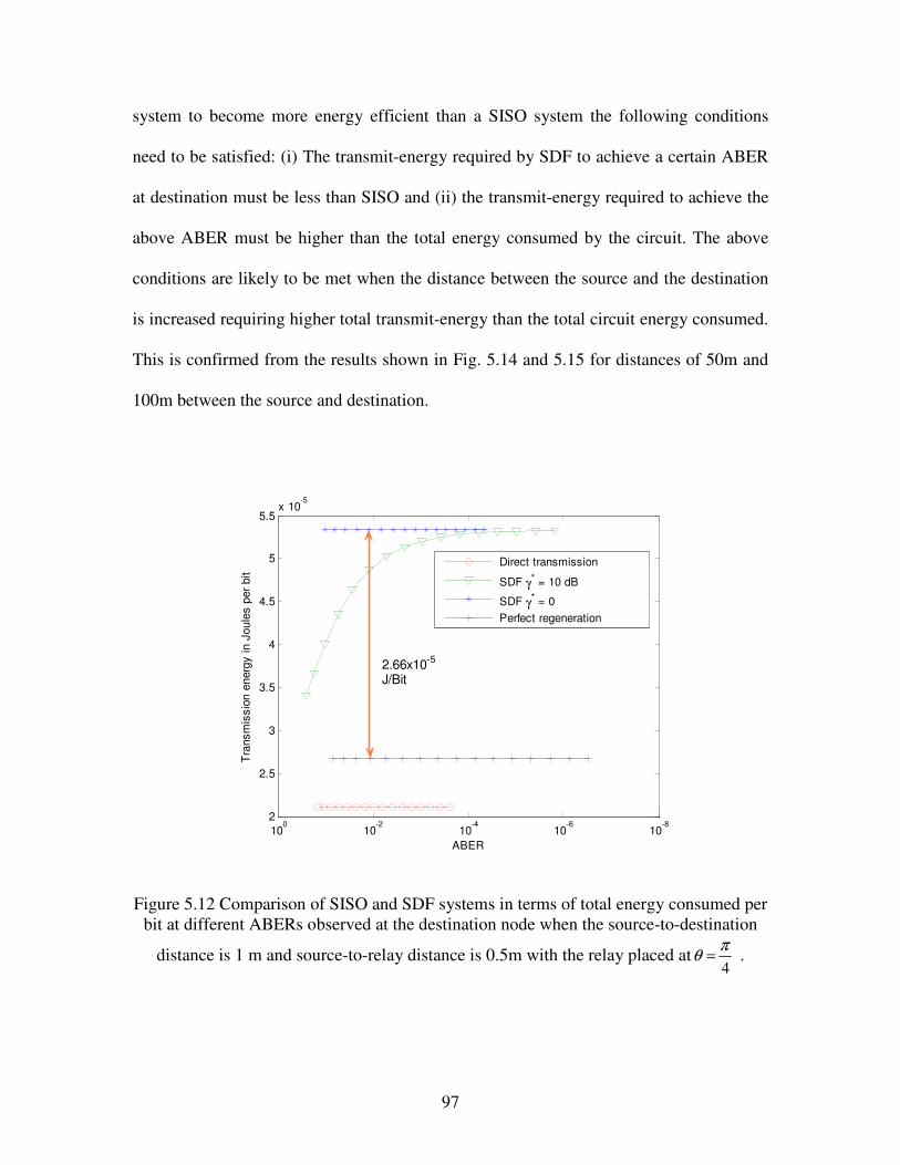
97

system to become more energy efficient than a SISO system the following conditions

need to be satisfied: (i) The transmit-energy required by SDF to achieve a certain ABER

at destination must be less than SISO and (ii) the transmit-energy required to achieve the

above ABER must be higher than the total energy consumed by the circuit. The above

conditions are likely to be met when the distance between the source and the destination

is increased requiring higher total transmit-energy than the total circuit energy consumed.

This is confirmed from the results shown in Fig. 5.14 and 5.15 for distances of 50m and

100m between the source and destination.

10-8

10-6

10-4

10-2

100

2

2.5

3

3.5

4

4.5

5

5.5x 10

-5

ABER

Tran

smis

sion

ene

rgy

in J

oule

s pe

r bit

Direct transmission

SDF γ* = 10 dB

SDF γ* = 0Perfect regeneration

2.66x10-5

J/Bit

Figure 5.12 Comparison of SISO and SDF systems in terms of total energy consumed per bit at different ABERs observed at the destination node when the source-to-destination

distance is 1 m and source-to-relay distance is 0.5m with the relay placed at4πθ = .

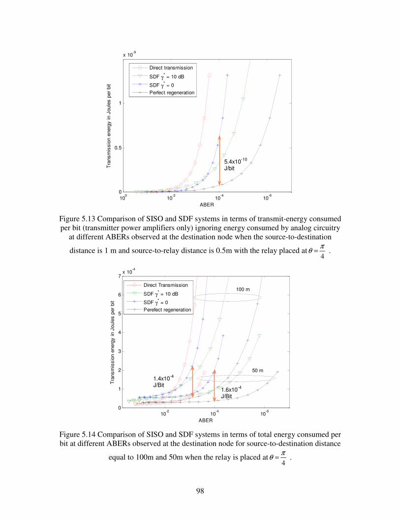
98

10-6

10-4

10-2

100

0

0.5

1

x 10-9

ABER

Tra

nsm

issi

on e

nerg

y in

Jou

les

per b

it

Direct transmission

SDF γ* = 10 dB


5.4x10-10

J/bit

Figure 5.13 Comparison of SISO and SDF systems in terms of transmit-energy consumed per bit (transmitter power amplifiers only) ignoring energy consumed by analog circuitry

at different ABERs observed at the destination node when the source-to-destination

distance is 1 m and source-to-relay distance is 0.5m with the relay placed at4πθ = .

10-6

10-4

10-2

0

1

2

3

4

5

6

7x 10

-4

ABER

Tran

smis

sion

ene

rgy

in J

oule

s pe

r bit

Direct Transmission

SDF γ* = 10 dB

SDF γ* = 0Perefect regeneration

100 m

50 m

1.4x10-4

J/Bit1.6x10-4

J/Bit

Figure 5.14 Comparison of SISO and SDF systems in terms of total energy consumed per bit at different ABERs observed at the destination node for source-to-destination distance

equal to 100m and 50m when the relay is placed at4πθ = .

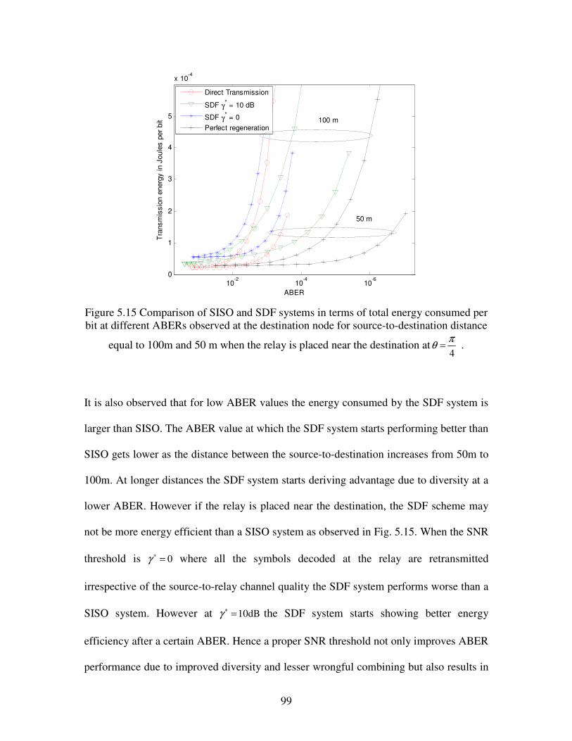
99

10-6

10-4

10-2

0

1

2

3

4

5

x 10-4

ABER

Tran

smis

sion

ene

rgy

in J

oule

s pe

r bi

t

Direct Transmission

SDF γ* = 10 dB


100 m

50 m

Figure 5.15 Comparison of SISO and SDF systems in terms of total energy consumed per bit at different ABERs observed at the destination node for source-to-destination distance

equal to 100m and 50 m when the relay is placed near the destination at4πθ = .

It is also observed that for low ABER values the energy consumed by the SDF system is

larger than SISO. The ABER value at which the SDF system starts performing better than

SISO gets lower as the distance between the source-to-destination increases from 50m to

100m. At longer distances the SDF system starts deriving advantage due to diversity at a

lower ABER. However if the relay is placed near the destination, the SDF scheme may

not be more energy efficient than a SISO system as observed in Fig. 5.15. When the SNR

threshold is 0γ ∗ = where all the symbols decoded at the relay are retransmitted

irrespective of the source-to-relay channel quality the SDF system performs worse than a

SISO system. However at 10dBγ ∗ = the SDF system starts showing better energy

efficiency after a certain ABER. Hence a proper SNR threshold not only improves ABER

performance due to improved diversity and lesser wrongful combining but also results in

100

lesser energy consumption. This also points to the importance of proper design choices

such as when to use cooperation and the choice of SNR threshold based on relay position.

Finally in all the figures 5.12-5.15, we have plotted the energy consumed by the SDF

system if it is assumed that the relay is able to perfectly regenerate all the symbols

transmitted by the source although the source (and the relay with transmit-power equal to

the source) transmits with power that is required to achieve the target ABER at the

destination due to diversity combing. We compare this to the scenario where the relay

retransmits with an SNR threshold 0γ ∗ = . In Fig. 5.12 the comparison shows that the

perfect regeneration assumption of SDF scheme is off by 52.66 10 J Bit−× , which is 50%

of the energy consumed in the practical SDF scenario with 0γ ∗ = . The energy efficiency

calculated in Fig. 5.13 under the perfect regeneration assumption is off by about 70 to

88 % corresponding to 41.4 10 J Bit−× for 100m and 41.6 10 J Bit−× for 50m respectively.

Moreover in the case where the relay is placed near the destination the perfect

regeneration always shows better performance than SISO whereas the SDF with 0γ ∗ =

never shows better energy efficiency than SISO. From the above it is clear that when

designing a cooperative system assuming perfect regeneration can lead to wrong design

choices in terms of energy efficiency.

5.5 Conclusions In this chapter, we presented analysis for computation of exact ABER for a simple SDF

scheme with BPSK modulation and a tight upper bound for symbol error rate for general

constellations. We have presented a unified analysis that can handle different geometry of

the nodes, non-identical fading characteristics over different hops and imperfect

regeneration at the relay. It was also shown through contour plots that there exists a

101

region of values of SNR threshold and values of fractional power allocated that produces

minimum ABER performance. This has motivated the idea of preferring higher SNR

threshold when operating in a network for improving spectral efficiency. The expression

for optimum SNR threshold that minimizes ABER performance was also derived and

argued to be easier for implementation as it only requires knowledge of average SNR per

link. In this chapter, we also examined the performance of cooperative communication in

terms of energy efficiency. It was shown that the energy consumed per bit by the SDF

system can be less than a SISO system when for a given average total transmit-energy the

ABER performance of SDF is better and when the total transmit-energy consumed

becomes higher than the total energy consumed by the analog circuit.

Having studied a simple SDF scheme based on SNR threshold at the relay, in the next

chapter we propose a maximum posteriori probability (MAP) relaying based SDF system

that performs better than SNR threshold with similar implementation complexity.

102

Chapter 6

6 Log-Likelihood-Ratio based Selective Decode and Forward Cooperative Communication

The purpose of this chapter is to present a selective decode and forward (SDF)

cooperative diversity system that uses a log likelihood ratio (LLR) threshold based

criterion at the relay to makes decisions on forwarding information. The main aim of this

chapter is to present the analysis of the LLR based SDF system for ABER performance

and to show that it performs better than a SNR threshold based SDF system discussed in

chapter 5. It is also shown that with optimal choice of LLR threshold the ABER

performance is comparable to optimal ML detection and C-MRC based cooperative

diversity with a much lower implementation complexity.

In the following sections we first explain the LLR criterion for a SISO system with BPSK

modulation and its relation to bit error rate and then provide an analysis for the end-to-

end ABER for the SDF system.

6.1 Log likelihood criterion

The concept of LLR based threshold and its relation to bit error rate for a SISO system is

explained in this section as derived in [124]. Assume that the signal received at the output

of a SISO channel is given by

y hx n= + (6.1)

103

The received signal is represented by y , the input signal is x which takes on values

sE+ or sE− with probability 0.5 , the channel gain between the transmitter and

receiver is h and n is the AWGN noise with zero mean and two sided power spectral

density 0 2N . The log-likelihood ratio Λ for x is given by

( )( )

0

, 4ln

,

s s

s

P x E h y Eh y

NP x E h y∗

= + Λ = = ℜ = −

(6.2)

where the sign of Λ is the hard decision value and the magnitude represents the reliability

of the hard decision. In the LLR based SDF scheme for cooperative communication the

relay forwards information based on a preset LLR threshold instead of a SNR threshold

described in chapter 5. In this case the relay makes decisions based on the reliability of

the decoded bit.

The bit error rate for the above system can be derived as follows. Let

( ) ( )( )

1ln

1

P x RR

P x R

= +Λ =

= − (6.3)

We already know that ( ) ( )1 1 1P x R P x R= + + = − = . This implies that

( ) ( )( )1

11 exp

P x RR

= + =+ −Λ

(6.4)

and

( ) ( )( )1

11 exp

P x RR

= − =+ Λ

(6.5)

The bit error probability is given by

104

( ) ( ) ( ) ( )ˆ ˆ ˆ1, 1 1, 1eP R P x x R P x x R P x x R= ≠ = = = − + = − = (6.6)

where x is the decision statistic. If ( ) 0RΛ > for ˆ 0x > then from (6.6)

( ) ( ) ( ) ( )( )0

1ˆ 1, 11 expe RP R P x x R

RΛ > = = = − =+ Λ

(6.7)

When ( ) 0RΛ < , it can be similarly shown that ( ) ( ) ( )( )0

11 expe RP R

RΛ > =+ −Λ

. Hence the

bit error probability is given by

( ) ( )1

1 expeP RR

=+ Λ

(6.8)

The expression in (6.8) is utilized in the following section to derive the end-to-end

probability of LLR based SDF scheme with the same system model as described in

section 5.1.

6.2 ABER performance analysis

The system model used for the SDF system is the same as explained in section 5.1 except

for the criterion used by the relay for forwarding the symbols received.

The error probability of the selective decode and forward scheme is dictated by three

mutually exclusive events which is given by

( ) ( ) ( ) ( )1 DIV XSD SR SRe e e ee e

P P F P P P P∗ ∗∗

Λ Λ>Λ Λ>Λ= ⋅ Λ + − ⋅ + ⋅ (6.9)

The first term on the RHS of (6.9) represents the event where there is no retransmission

from the relay as the LLR is below the preset threshold denoted by ∗Λ represented by the

105

CDF ( ) ( )PrF ∗ ∗Λ Λ = Λ < Λ .Thus the detection at the destination is solely based on

probability of symbol error in source-to-destination link represented by SDeP . The second

and third terms represent the event where the relay decodes and decides to forward in the

relay phase. The second term represents the case where the relay correctly decoded the

symbol transmitted from the source in the broadcast phase with probability

( )1 SR

eP ∗Λ>Λ

− and in relay phase after coherent diversity combining of the two received

signals at the destination, the transmitted symbol is decoded in error with

probability ( )DIVeP . The third term represents the case where the relay in the broadcast

phase decodes the symbol transmitted from the source in error with probability SR

eP ∗Λ>Λ

.

This can happen due to improper choice of threshold level. This leads to wrongful

combining at the destination in phase two where ( )XeP denotes the probability of error due

to wrongful combining.

The probability of error SDeP in (6.9) can now be computed as

( ) ( ) ( )2

20

1 1,

sinSD SD

SDe eP P f d d

π

γ γγ

γ γ γ φ γ θπ θ∗

∞∗

= =

(6.10)

where ( )SDγφ ⋅ is the MGF of the instantaneous received SNR SDγ which is readily

available in closed form for Rayleigh fading [124]. Following the treatment in [78],

( )DIVeP can be computed as

( )

( ) ( )1 2

2 20

1 1 1sin sinSD RD

DIVeP dγ γφ φ θ

π θ θ

=

(6.11)

The decision statistic as a result of wrongful combining can be written as

106

( ) ( ) 2 2 2 2ˆ 1 1D T SD SD T RD RD T SD SD SD T RD RD RDZ E E E n E nδ σ α δ σ α δ σ α δ σ α∗ ∗= − − + ℜ + − (6.12)

The bit error probability for the decision statistic in (6.12) can now be evaluated as

( )1 2

XeP P P= + where

( )( ) ( )

( ) ( )

2 2 2 21 2 2 2 2

00 1

2 11

1

RD

SD RD

TSD SD RD RD

SD SD RD RD

SD RD SD RD

EP Q

N

f f d d

δαδ

α α

δσ α δ σ αδσ α δ σ α

α α α α

∞ ∞

−

= − −

+ −

×

(6.13)

And

( )( ) ( )( ) ( )

1

2 2 2 22 2 2 2 2

00 0

2 11 1

1

RD

SD RD

TRD RD SD SD

SD SD RD RD

SD RD SD RD

EP Q

N

f f d d

δαδ

α α

δ σ α δσ αδσ α δ σ α

α α α α

−∞

= − − − + −

×

(6.14)

Now we turn our attention to the LLR threshold based forwarding at the relay. For BPSK

modulation the decision statistic is given by

2ˆSR SR SR SR S S SR SRZ r E b nα α α∗ ∗= ℜ = + ℜ (6.15)

As explained in section 6.1 the LLR Λ for this receiver can also be derived as

ˆ4 SR SZ EΛ = [124]. Now if we let ˆS SRh E Z= and thus 4hΛ = then for Rayleigh fading

channel the PDF of h is given by [124]

( )2

1 1exp 2 1 1 exp 2 1 1

h

h h

f hβ β

β β

− + + + − + − =

+ (6.16)

where 2SR sE Eβ α= . Now SR

eP ∗Λ>Λ

can be computed as

107

( ) ( )

4

11 exp 4

SRhe

P f h dhh

∗

∗

∞

Λ>ΛΛ

=+ (6.17)

The CDF ( ) ( )PrF ∗ ∗Λ Λ = Λ < Λ can also be evaluated as [124]

( ) ( ) ( ) ( )4

2 20

2 1 2 11 exp 1 1 1 exp 1 1

4 4

2 1 2 1hF f h dh

β β

β β β β β β

∗

∗ ∗

Λ∗

Λ

− Λ − Λ− + + − + − Λ = = +

+ + + + − + (6.18)

Using (6.10)-(6.18) the computation of end-to-end ABER in (6.9) can be completed. Next

the derivation of optimum LLR threshold is discussed.

6.3 Optimal LLR threshold

From (6.9) it can be observed that an optimum ∗Λ to produce the minimum eP can be

obtained by minimizing the ABER in (6.9). Noting that,

( ) ( )b

a

df x f a

da= − and ( ) ( )

b

a

df x f b

db= ; we can derive optimum ∗Λ by taking the

derivative of (6.9) and equating it to zero. The derivative of (6.9) is given by

( )

( )( )

( )( ) ( )( )

( )

1 1 1 1 14 4 4 4 4 41 exp 1 exp

1

4 4 1 exp

DIV XSDee h e h e h

DIV Xe eSD

h e

dPP f P f P f

d

P Pf P

∗ ∗ ∗

∗ ∗ ∗

∗

∗

Λ Λ Λ = − − + − Λ + Λ + Λ

− Λ = + + Λ (6.19)

108

Equating (6.19) to zero and observing that 04hf

∗ Λ ≥

, the optimum SNR threshold is

obtained when ( ) ( ) ( )1

1 exp

SDe

X DIVe eopt

P

P P∗=

−+ Λand the optimum LLR is given by

( ) ( )ln 1

X DIVe e

opt SDe

P PP

∗ −Λ = −

. Note that evaluation of opt∗Λ only requires the knowledge of

bit error probabilities, ( )XeP , ( )DIV

eP and SDeP . These can either be feedback from the

destination to the relay or the average received SNR on each link can be to the relay to

make the computations at the relay. The above method does not require knowledge of

instantaneous received SNRs and hence is more desirable from an implementation

standpoint.

6.4 Results

Fig. 6.1 shows the plots for the performance comparison of the DF scheme that results in

optimum ABER performance using ML detection at the destination [23], C-MRC [114],

SDF scheme based on SNR threshold at the relay and the SDF scheme with LLR

threshold based relay. The parameters for the system model with reference to Fig. 5.1

are 3µ = , 1SDd = , 0.5RDd = and 1.25 cos4SRdπ = −

. The figure also includes plots of

ABER for different values of LLR thresholds and SNR threshold levels. It can be

observed that LLR based scheme outperforms the simple SNR threshold based SDF

scheme as it is based on a better decision metric at the relay. The optimum LLR

computed using the derivation in section 6.3 shows an ABER performance that is

approximately 1 dB worse than optimum ML based DF scheme [23] and C-MRC [114].

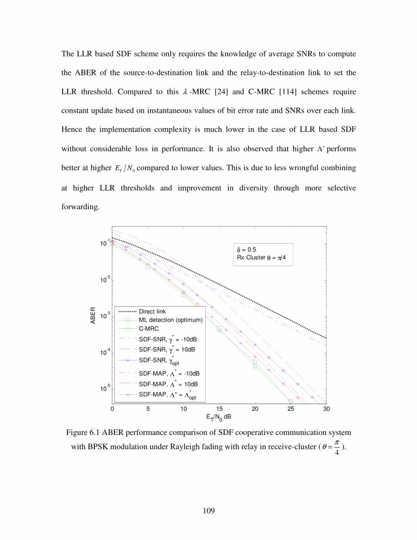
109

The LLR based SDF scheme only requires the knowledge of average SNRs to compute

the ABER of the source-to-destination link and the relay-to-destination link to set the

LLR threshold. Compared to this λ -MRC [24] and C-MRC [114] schemes require

constant update based on instantaneous values of bit error rate and SNRs over each link.

Hence the implementation complexity is much lower in the case of LLR based SDF

without considerable loss in performance. It is also observed that higher ∗Λ performs

better at higher 0TE N compared to lower values. This is due to less wrongful combining

at higher LLR thresholds and improvement in diversity through more selective

forwarding.

0 5 10 15 20 25 30

10-5

10-4

10-3

10-2

10-1

ET/N0 dB

AB

ER Direct link

ML detection (optimum)C-MRC

SDF-SNR, γ* = -10dB

SDF-SNR, γ* = 10dB

SDF-SNR, γ*opt

SDF-MAP, Λ* = -10dB

SDF-MAP, Λ* = 10dB

SDF-MAP, Λ* = Λ*opt

δ = 0.5Rx Cluster θ = π/4

Figure 6.1 ABER performance comparison of SDF cooperative communication system

with BPSK modulation under Rayleigh fading with relay in receive-cluster (4πθ = ).

110

6.5 Conclusions

In this chapter we derived an efficient method to compute the ABER of a SDF based

cooperative diversity system under Rayleigh fading that uses a LLR based threshold

criterion at the relay to forwards symbols. ABER performance comparison showed that

the LLR based SDF system performs about 1 dB worse than the optimum DF system at

considerably low implementation complexity.

111

Chapter 7

7 A practical application of cooperative communication: cooperative relaying for ad-hoc ground networks using swarm UAVs

In this chapter we look at the feasibility of a practical application of some of the

cooperative relaying techniques suggested in the literature. Unmanned aerial vehicles

(UAVs) have recently gained the attention as dispensable autonomous vehicles for

relaying sensor data for aerial surveillance during military operations. An emerging

application is the use of small UAVs as relay nodes to form reliable communication links

for ad-hoc ground networks in tactical situations. Field tests were conducted in [94] using

a wireless node onboard a single UAV for an 802.11b ad-hoc ground network with fixed

nodes. The results show that the throughput using a UAV based relay increases by a

factor of two and connectivity improves by 67% when compared to the ad hoc ground

network without using the UAV.

Use of antenna arrays with multiple-input-multiple-output (MIMO) signal processing

techniques has been known to give tremendous improvements in the performance of

point-to-point communication links [13]. Unfortunately the cost, weight, and poor design

of antenna arrays prohibit their use on low cost unmanned vehicles. Recently,

communication using cooperation between multiple wireless nodes acting as virtual

antenna elements have been studied with the promise of improved capacity and better

reliability than single links. It was also reported in [95], that ongoing efforts with

coordinated UAV flights have succeeded in flying two UAVs in pre-programmed

112

positions that can communicate with each other about their respective positions.

Technological advances such as this and ongoing research on swarming of small low cost

UAVs make multi-UAV formation flights a near term reality. This brings up an

interesting possibility of exploiting cooperative communication between UAVs with

single antenna wireless nodes to improve reliability and range of ad hoc ground networks.

In [62] the authors have analyzed the performance of distributed beamforming by

cooperation between nodes for a wireless sensor networks. In this chapter we apply the

idea of distributed transmit beamforming [62] and distributed orthogonal space-time

block codes (OSTBC) as described in chapter 5, to cooperative UAV assisted relaying for

fixed ad-hoc ground networks. We specifically evaluate the performance of two-hop

multiple UAV relay system under non-ideal conditions like turbulence on UAVs which

cause position and phase errors are evaluated for transmit beamforming.

The following gives a brief outline of this chapter. In section 7.1 we describe the

motivation and background behind UAV based communication. In section 7.2 we discuss

the air-to-ground channel characteristics and models reported in literature to justify their

use in simulation. Section 7.3 discusses the characteristics of UAV flight that can

potentially affect the performance of communication links. In section 7.4 the simulation

set-up is explained. Section 7.5 shows results from simulation of distributed transmit

beamforming and distributed OSTBC schemes under ideal conditions. It also shows the

effect of position error and Doppler due to turbulence on the performance of distributed

transmit beamforming. Conclusions are drawn in section 7.7.

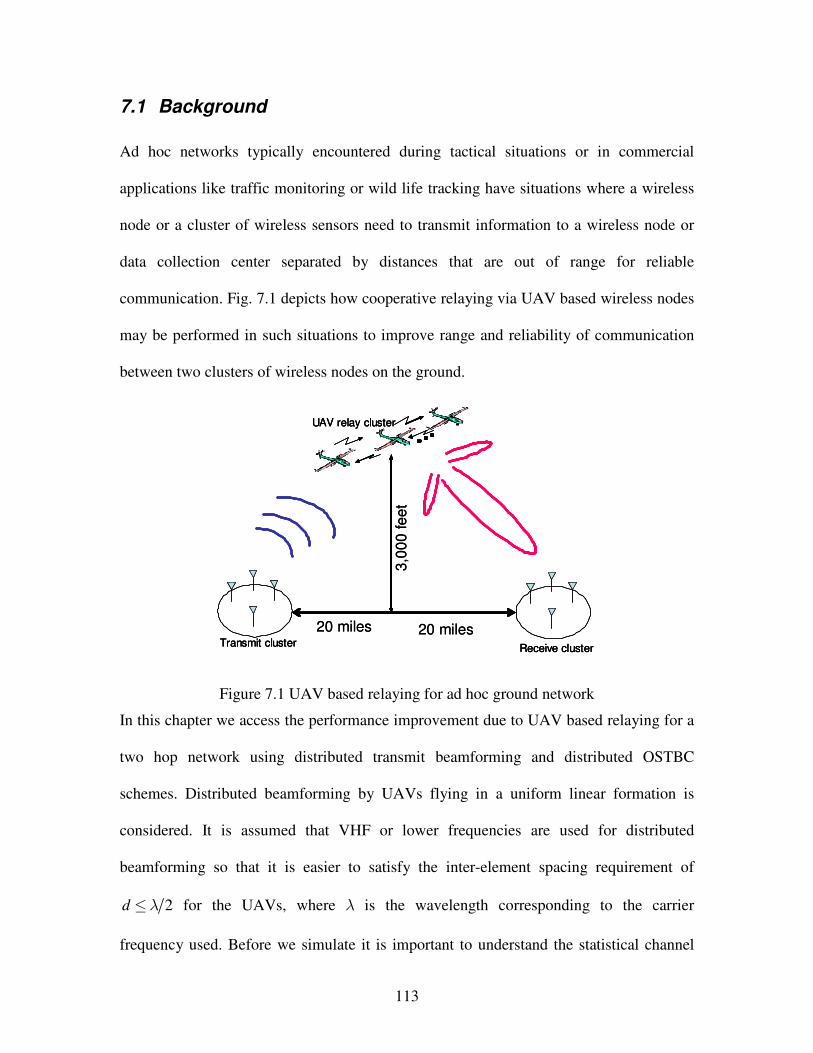
113

7.1 Background

Ad hoc networks typically encountered during tactical situations or in commercial

applications like traffic monitoring or wild life tracking have situations where a wireless

node or a cluster of wireless sensors need to transmit information to a wireless node or

data collection center separated by distances that are out of range for reliable

communication. Fig. 7.1 depicts how cooperative relaying via UAV based wireless nodes

may be performed in such situations to improve range and reliability of communication

between two clusters of wireless nodes on the ground.

Transmit cluster Receive cluster

UAV relay cluster

3,00

0 fe

et

20 miles 20 milesTransmit cluster Receive cluster

UAV relay cluster

Transmit cluster Receive cluster

UAV relay cluster

3,00

0 fe

et

20 miles 20 miles

Figure 7.1 UAV based relaying for ad hoc ground network

In this chapter we access the performance improvement due to UAV based relaying for a

two hop network using distributed transmit beamforming and distributed OSTBC

schemes. Distributed beamforming by UAVs flying in a uniform linear formation is

considered. It is assumed that VHF or lower frequencies are used for distributed

beamforming so that it is easier to satisfy the inter-element spacing requirement of

2d % for the UAVs, where is the wavelength corresponding to the carrier

frequency used. Before we simulate it is important to understand the statistical channel

114

models applicable to the scenario under consideration. Communication using UAVs

involves air-to-ground communication. In the next section we look at statistical channel

models and path loss exponents suggested for air-to-ground communication links in

literature.

7.2 Statistical channel models and path loss exponent for UAV

based communication

7.2.1 Statistical air-to-ground channel models

Aeronautical (air-to-ground) channel characterization based on measurements made

during flight tests was first reported in [96]. The mathematical model used link geometry

and surface roughness to describe the received signal. The measurement was done at a

carrier frequency of 1463 MHz and elevation angles of 0.5-45°. In [97] the authors

characterized a satellite-to-ship channel based on extensive measurements at 1530-1545

MHz. Their suggestions for the channel model include a stochastic channel model based

on Rice distribution for amplitude of the received signal envelope with a Rice K-factor of

4-5 dB at 1° elevation and increasing up to 20 dB for higher elevation angles. In [98] a

stochastic model based on Rice distribution is suggested based on flight measurement

results at VHF frequencies. The measurements were taken at an altitude of 4000 feet, a

radius of 18 miles and at a speed of 270 miles per hour. [99] also suggests a Rice channel

model for measurements taken on flights at 440m/s (850 knots). They observe that the

average Rice K-factor observed is 15 dB with the worst case being 2 dB. Measurements

in [100 suggest frequency selective fading due to large delay spreads at low K factors. In

115

all of the above cases, measurements were made using continuous wave (CW) signals.

The following describe measurement results with sliding correlator type systems.

Measurements in [101] used an airborne transmitter to characterize multipath propagation

at 1820 MHz for spread-spectrum satellite communications. A sliding correlator system

with PN sequences at a chip rate of 10 MHz and 30 MHz was used. The measurement

data indicated that multipath components could be divided among three regions in the

power-delay profiles: direct path, near echoes, and far echoes. The amplitude of the

direct-path component was shown to be Rice distributed in LOS conditions with K-factor

between 10 - 30 dB and Rayleigh distributed in shadowed regions. In the near-echo

region (0-600 ns), the amplitude of components decreased exponentially with delay, and

the delay of the components was exponentially distributed. A majority of the multipath

components appeared in the near echo region. In [102] a sliding correlator system was

used to measure narrowband and wideband channel characteristics in the VHF

aeronautical communications band at 135 MHz. Their results again show that the channel

is predominantly Rician with large K-factors (2.9 dB – 19.7 db) with insignificant

amount of small scale fading.

From the above survey on propagation measurements the following are some common

features that emerge for air-to-ground channels, which can be assumed for simulation of

relay channels using UAVs.

Existence of multipath in the air-to-ground channel is dependent upon the environment

surrounding the ground-based receiver. Small elevation angles result in richer multipath

content.

116

The air-to-ground channel is predominantly Rician with large K-factors although large

excess delays can be expected in air-to-ground channels

In the case of low cost UAVs the average altitude is assumed to be 3000 feet with a

navigational range of about 20 miles. Assuming transmission at the edge of this range the

elevation is around 1°. Hence we assume Rice distribution for simulating the amplitude

of received signal envelope with a maximum Rice K-factor of 4.77 dB or K = 3. Since

the elevation is low it is assumed that the channel is also rich in multipath.

7.2.2 Path loss exponent

Propagation in air under line of sight (LOS) is usually considered to be equivalent to

propagation in free space with a path loss exponent of 2n . For air-to-ground

communication there are additional reflected signals from the surface of the earth, which

can affect the signal strength at the receiver. The path loss exponent is independent on the

frequency used, but its relation to altitude and distance between transmitter and receiver

can vary for air-to-ground propagation. In [102] the authors report a path loss exponent of

2 in one of the locations and around 4 at another location for large distances of air-to-

ground measurements indicating that the type of surface near the receiver affects large

scale fading (shadowing). In [103] the authors have shown the dependence of path loss

exponent on altitude and distance between transmitter and receiver based on

measurements performed using VHF and UHF bands. The altitude of the transmitter

varied from 0 to 2000 feet and the distance varied from 0-40 miles. At a height of 2000

feet the path loss exponent, n varies from less than 2 to 2.3. It is also shown that as the

height of the transmitter increases from 0 to 2000 feet n decreases from 2.4 to 2 at a

distance of 40 miles. For our simulations the path loss exponent is assumed to be 2n .

117

The next section discusses the characteristics of UAV flight, which need to be considered

for simulation setup.

7.3 UAV flight characteristics

UAVs have limited range of operation due to their size and navigational needs. They are

also subject to turbulence due to wind at different altitudes. As such the communication

systems on board especially with multi-UAV formation flights will be subject to position

errors, Doppler shifts due to different UAV relative velocities and timing errors. To

account for these in simulation we document some of the characteristics of UAV flight,

which would help us, set up the simulation parameters as well as look at performance

under worst-case scenarios. The following summarizes the characteristics on UAVs

important for simulation:

• Wing span 3-4 ft

• Maximum speed 109 km/hr (68 miles/hr) [94], [104], [105]

• Maximum altitude 3,000 ft (914.4m) (assumed) [106]

• Maximum range 20 miles

• Maximum wind speed 22 knots (40.74 Km/Hr) [106]

• At 10 knots, maximum lateral displacement = 1.7 feet in 3s [106]. Therefore at 22

knots maximum lateral displacement is assumed to be 3 feet

• Due to turbulence vertical maximum average displacement = 3 feet

• Maximum Transmitted Power 1 W [94]

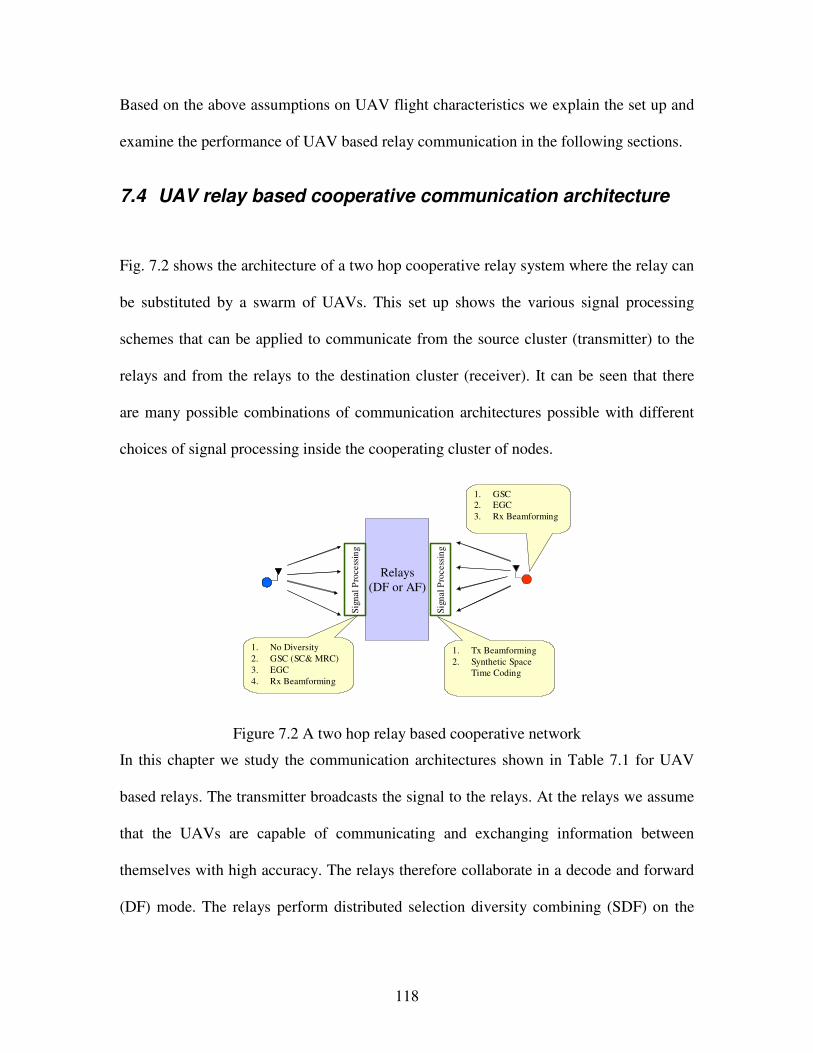
118

Based on the above assumptions on UAV flight characteristics we explain the set up and

examine the performance of UAV based relay communication in the following sections.

7.4 UAV relay based cooperative communication architecture

Fig. 7.2 shows the architecture of a two hop cooperative relay system where the relay can

be substituted by a swarm of UAVs. This set up shows the various signal processing

schemes that can be applied to communicate from the source cluster (transmitter) to the

relays and from the relays to the destination cluster (receiver). It can be seen that there

are many possible combinations of communication architectures possible with different

choices of signal processing inside the cooperating cluster of nodes.

Relays(DF or AF)

Sign

al P

roce

ssin

g

Sign

al P

roce

ssin

g

1. No Diversity2. GSC (SC& MRC)3. EGC4. Rx Beamforming

1. Tx Beamforming2. Synthetic Space

Time Coding

1. GSC2. EGC3. Rx Beamforming

Figure 7.2 A two hop relay based cooperative network

In this chapter we study the communication architectures shown in Table 7.1 for UAV

based relays. The transmitter broadcasts the signal to the relays. At the relays we assume

that the UAVs are capable of communicating and exchanging information between

themselves with high accuracy. The relays therefore collaborate in a decode and forward

(DF) mode. The relays perform distributed selection diversity combining (SDF) on the

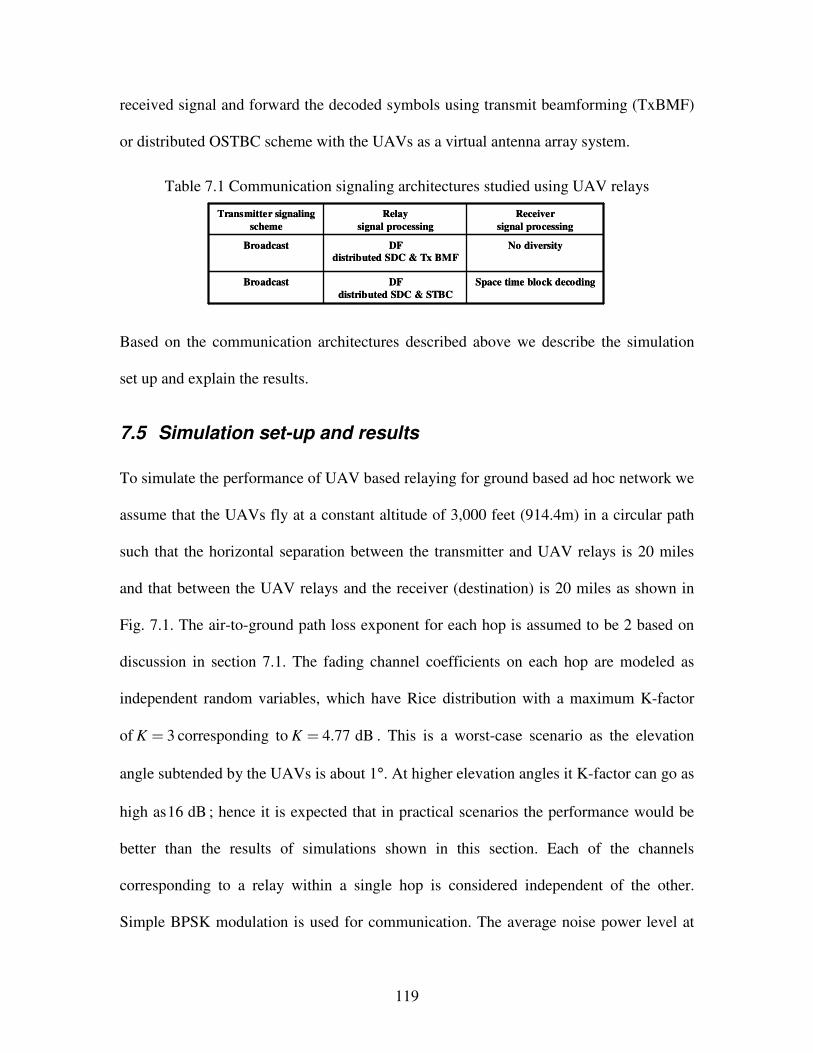
119

received signal and forward the decoded symbols using transmit beamforming (TxBMF)

or distributed OSTBC scheme with the UAVs as a virtual antenna array system.

Table 7.1 Communication signaling architectures studied using UAV relays

Space time block decodingDFdistributed SDC & STBC

Broadcast

No diversityDFdistributed SDC & Tx BMF

Broadcast

Receiver signal processing

Relaysignal processing

Transmitter signaling scheme

Space time block decodingDFdistributed SDC & STBC

Broadcast

No diversityDFdistributed SDC & Tx BMF

Broadcast

Receiver signal processing

Relaysignal processing

Transmitter signaling scheme

Based on the communication architectures described above we describe the simulation

set up and explain the results.

7.5 Simulation set-up and results

To simulate the performance of UAV based relaying for ground based ad hoc network we

assume that the UAVs fly at a constant altitude of 3,000 feet (914.4m) in a circular path

such that the horizontal separation between the transmitter and UAV relays is 20 miles

and that between the UAV relays and the receiver (destination) is 20 miles as shown in

Fig. 7.1. The air-to-ground path loss exponent for each hop is assumed to be 2 based on

discussion in section 7.1. The fading channel coefficients on each hop are modeled as

independent random variables, which have Rice distribution with a maximum K-factor

of 3K corresponding to 4.77 dBK . This is a worst-case scenario as the elevation

angle subtended by the UAVs is about 1°. At higher elevation angles it K-factor can go as

high as16 dB ; hence it is expected that in practical scenarios the performance would be

better than the results of simulations shown in this section. Each of the channels

corresponding to a relay within a single hop is considered independent of the other.

Simple BPSK modulation is used for communication. The average noise power level at

120

each of the receivers in each hop is assumed to be -100 dBm. The transmit power at the

source (PTx) is varied from 0 to 30 dBm. The transmit power at each relay is a fraction

of the transmit power of the source. This fraction is given by 1/L where L is the total

number of UAV relays used.

Distributed transmit beamforming at the relays assumes that each relay has perfect

knowledge about the channel state information between the relay and the receiver. This

may be assured by introducing channel state feedback mechanism from the destination to

the relays or by applying reciprocity and using channel estimates calculated by each relay.

The effect of channel estimation errors on the performance is out of scope of this chapter.

The signal received at the destination receiver due to distributed transmit beamforming

can be written as

Hr s n w w (7.1)

where w is a vector representing the channel coefficients corresponding to each relay-

receiver link which is used as beamforming weights by the relay, s is the relayed symbol

and n represents AWGN noise. Passing the received signal through a matched filter then

results in the required signal statistic. It is assumed that all transmitting nodes are

triggered at the same time using GPS clocks on board a UAV.

For transmit OSTBC we consider orthogonal G2 and G4 schemes described in [72]. Each

UAV relay is assumed to transmit a column of symbols that corresponds to the block

code. To give an example the received signal due to G2 OSTBC scheme is given by (7.2).

1 1 1 2 2 1

2 1 2 2 1 2

r h s h s n

r h s h s n) )

(7.2)

121

where 1r and 2r are received signals during two consecutive symbol durations, 1h and 2h are

fading channel coefficients corresponding to the two transmit-receive channels

respectively, 1s and 2s are consecutive symbols encoded using OSTBC,

and 1n and 2n correspond to AWGN noise corresponding to the received signals. It is

assumed that the symbols undergo flat fading, which remains constant for the duration of

the block of symbols. Flat fading with duration similar to the OSTBC block is considered

for fair comparison with distributed transmit beamforming.

Fig. 7.3 shows the BER performance of a two-hop system using two and four UAV

relays. It is assumed that there are no errors due to synchronization or inter element

(UAV) position error arising from turbulence. The Rice K-factor considered on both hops

is equal to 4.77 dB (K = 3). The plot also shows the performance of a direct link between

the source and the destination for the same range. The path loss exponent assumed for

direct link is equal to 3 with Rayleigh fading channel model. The performance of a single

UAV (DF) relay system is also plotted where the UAV decodes the received signal and

retransmits it with power PTx. Hence the total power transmitted in all relay based cases

is 2PTx where PTx is the transmitted total power of the source.

From the simulation results it can be observed that there is a drastic improvement in BER

performance even with single DF UAV based relay. This also relates to a huge increase

in range which is about 35 times the range achieved with direct link with the same

transmit power. This can be attributed to the reduced effective path loss in aerial LOS

propagation using relays. It can be seen that with four UAV relays a gain of 11 dB is

achieved at BER of 110 with distributed transmit beamforming and a gain of 8 dB with

distributed OSTBC using G4 scheme. It should be noted however that the G4 OSTBC

122

scheme has a code rate of 1/2 whereas that of G2 is 1. Distributed transmit beamforming

performs better than distributed OSTBC. However it should be noted that distributed

beamforming requires that the received signals be coherent which in the case of a linear

formation with UAVs requires that they be uniformly separated by a distance 2d % ;

being the wavelength corresponding to the carrier frequency used. Hence depending on

the dimensions of a UAV, carrier frequencies at VHF or lower may be practical for

distributed transmit beamforming.

0 5 10 15 20 25 3010

-5

10-4

10-3

10-2

10-1

100

direct ground link1 UAV2 UAV OSTBC4 UAV OSTBC2 UAV BMF4 UAV BMF

Transmit power in dBm

BE

R

Figure 7.3 BER performance comparisons of two-hop UAV relay system with Rice K-factor = 4.77 dB

Next we consider the effect of varying Rice K-factor in one of the hops, on the

performance. Since the UAVs are collocated it is assumed that each link in a hop

experiences Rice fading with the same K-factor. Fig. 7.4 and Fig. 7.5 shows the effect of

different K-factors in the second hop for distributed transmit beamforming and

distributed OSTBC respectively. The values .1,1 and 3K were chosen. The K factor in

123

the first hop is kept constant at 3K . It can be seen that in the case of distributed

transmit beamforming K factor does not have any effect on the performance where as

transmit OSTBC, which depends on diversity, the performance degrades with lower K

factors. This is expected since diversity scheme looks at concentrating the PDF of the

received signal SNR at the mean of the PDF whereas beamforming tries to improve the

mean SNR and is only dependent o the beamforming weights. The improvement in

performance in Fig. 7.5 using distributed OSTBC for 3K is 4 dB and for 0.1K is 7dB

at a BER of 210 when going from two UAVs to four UAVs. The relative improvement

in performance for diversity is higher when there are more specular components at a low

K-factor. Hence use of distributed OSTBC or other distributed diversity schemes with

higher number of UAVs to derive higher diversity gain is better suited for a multipath

rich environment.

Next we look at the effect of Doppler and position errors on the performance of tow-hop

UAV based relay with distributed transmit beamforming. The signal transmitted from

each relay can be written as

02 ej f f ti ix t w s t e * ) (7.3)

where iw) is the complex conjugate weight corresponding to the fading channel

coefficient, s t is the transmitted symbol and f* is the shift in frequency due to Doppler

arising from differential wind speed between UAVs and e is the error in phase due to

error in position of the UAV in a linear array.

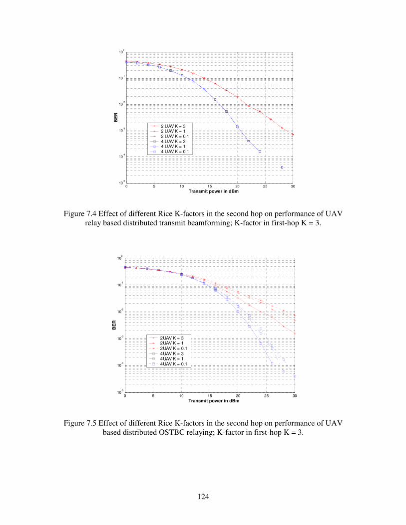
124

0 5 10 15 20 25 3010

-5

10-4

10-3

10-2

10-1

100

2 UAV K = 32 UAV K = 12 UAV K = 0.14 UAV K = 34 UAV K = 14 UAV K = 0.1


BE

R

Figure 7.4 Effect of different Rice K-factors in the second hop on performance of UAV relay based distributed transmit beamforming; K-factor in first-hop K = 3.

0 5 10 15 20 25 3010

-5

10-4

10-3

10-2

10-1

100

2UAV K = 32UAV K = 12UAV K = 0.14UAV K = 34UAV K = 14UAV K = 0.1


BE

R

Figure 7.5 Effect of different Rice K-factors in the second hop on performance of UAV based distributed OSTBC relaying; K-factor in first-hop K = 3.

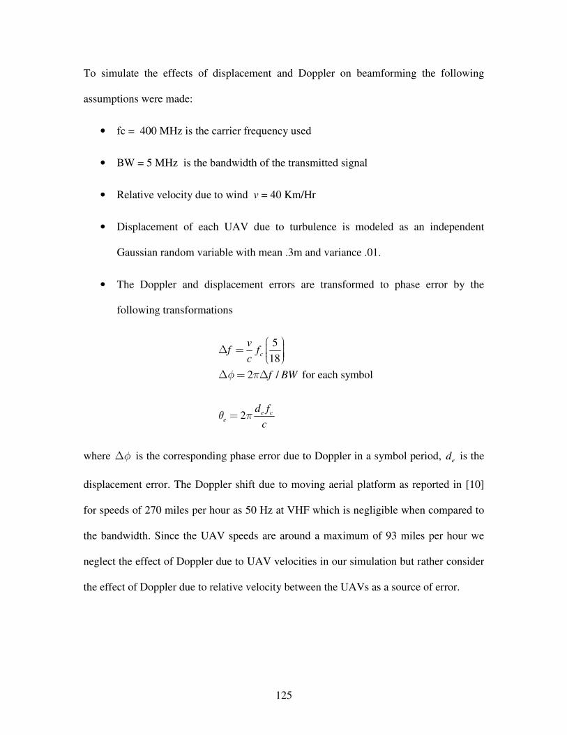
125

To simulate the effects of displacement and Doppler on beamforming the following

assumptions were made:

• fc = 400 MHz is the carrier frequency used

• BW = 5 MHz is the bandwidth of the transmitted signal

• Relative velocity due to wind v = 40 Km/Hr

• Displacement of each UAV due to turbulence is modeled as an independent

Gaussian random variable with mean .3m and variance .01.

• The Doppler and displacement errors are transformed to phase error by the

following transformations

5

182 / for each symbol

c

vf f

cf BW

*

* *

2 e ce

d fc

where * is the corresponding phase error due to Doppler in a symbol period, ed is the

displacement error. The Doppler shift due to moving aerial platform as reported in [10]

for speeds of 270 miles per hour as 50 Hz at VHF which is negligible when compared to

the bandwidth. Since the UAV speeds are around a maximum of 93 miles per hour we

neglect the effect of Doppler due to UAV velocities in our simulation but rather consider

the effect of Doppler due to relative velocity between the UAVs as a source of error.

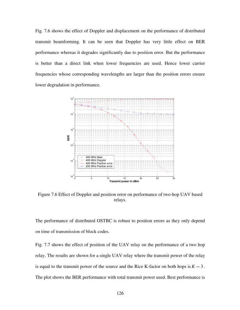
126

Fig. 7.6 shows the effect of Doppler and displacement on the performance of distributed

transmit beamforming. It can be seen that Doppler has very little effect on BER

performance whereas it degrades significantly due to position error. But the performance

is better than a direct link when lower frequencies are used. Hence lower carrier

frequencies whose corresponding wavelengths are larger than the position errors ensure

lower degradation in performance.

0 5 10 15 20 25 3010

-5

10-4

10-3

10-2

10-1

100

400 MHz Ideal400 MHz Doppler400 MHz Position error200 MHz Position error


BE

R

Figure 7.6 Effect of Doppler and position error on performance of two-hop UAV based relays.

The performance of distributed OSTBC is robust to position errors as they only depend

on time of transmission of block codes.

Fig. 7.7 shows the effect of position of the UAV relay on the performance of a two hop

relay. The results are shown for a single UAV relay where the transmit power of the relay

is equal to the transmit power of the source and the Rice K-factor on both hops is 3K .

The plot shows the BER performance with total transmit power used. Best performance is

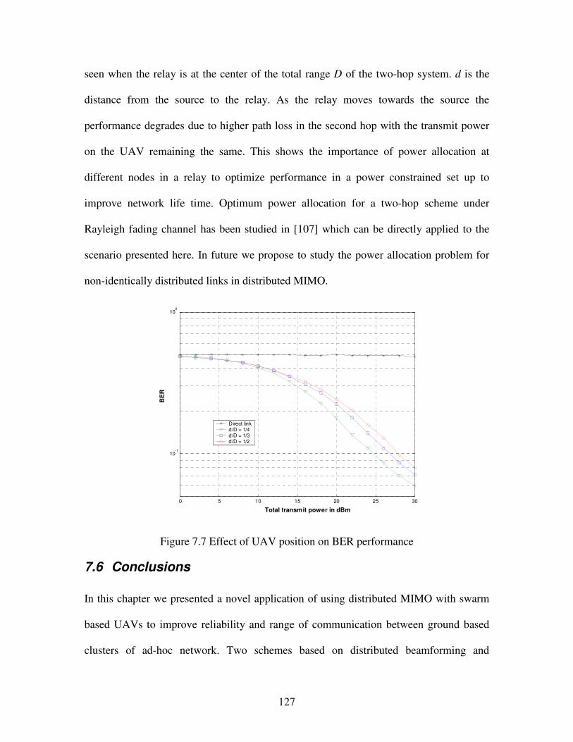
127

seen when the relay is at the center of the total range D of the two-hop system. d is the

distance from the source to the relay. As the relay moves towards the source the

performance degrades due to higher path loss in the second hop with the transmit power

on the UAV remaining the same. This shows the importance of power allocation at

different nodes in a relay to optimize performance in a power constrained set up to

improve network life time. Optimum power allocation for a two-hop scheme under

Rayleigh fading channel has been studied in [107] which can be directly applied to the

scenario presented here. In future we propose to study the power allocation problem for

non-identically distributed links in distributed MIMO.

0 5 10 15 20 25 30

10-1

100

Direct linkd/D = 1/4d/D = 1/3d/D = 1/2

Total transmit power in dBm

BE

R

Figure 7.7 Effect of UAV position on BER performance

7.6 Conclusions

In this chapter we presented a novel application of using distributed MIMO with swarm

based UAVs to improve reliability and range of communication between ground based

clusters of ad-hoc network. Two schemes based on distributed beamforming and

128

distributed OSTBC for two-hop relay communications were described. The BER

performances of the two schemes were compared. The effect of different Rice K-factors

was examined. Simulation results were described to show the effect of position errors on

the performance of distributed beamforming. It was shown that to achieve better

performance with distributed beamforming use of lower carrier frequencies (VHF and

below) is required. The effect of position of a UAV on the performance of a two hop

system was simulated which, shows the significance of power allocation strategies in a

distributed set up to achieve optimum performance. Based on simulation results presented

in this chapter it can be said that swarm UAV based multi-hop cooperative relaying can

improve the performance of ad-hoc ground networks. They can especially prove useful in

tactical scenarios where they can improve range and reliability of communication

drastically when compared to a direct link.

129

Chapter 8

8 Frequency domain based ABER analysis for bandlimited BPSK system with time synchronization error

Practical wireless communication systems are subject to the effects of fading, timing

error and cochannel interference from adjacent cells especially in a microcellular

environment. In this chapter we provide an analysis of the ABER of a bandlimited SISO

system with asynchronous cochannel interference under generalized fading channels that

makes use of the frequency domain based approach developed in chapter 8. Bit error

probability (BEP) for a bandlimited BPSK system due to ISI arising from timing error

was first analyzed using characteristic function (CHF) method in [80] and [81] for slow

and fast Rayleigh fading channels respectively. In [82] the authors presented analysis for

ABER of a bandlimited QPSK system with Rayleigh faded cochannel interferers using a

Fourier series approximation method. Recently in [83], using a method similar to that in

[80] a precise ABER was derived for a bandlimited BPSK system with asynchronous

cochannel interferers under slow Nakagami-m fading channels. The analysis allowed for

different fading severity indexes to be applied to the desired user and to each of the

interfering signals. Most of the previous works until [83] approached the analysis by

assuming that all the interfering signals underwent Rayleigh fading or derived

approximate solutions for the case where interfering signals were assumed to undergo

Rice fading. These results are well summarized in [83].

130

In this chapter we provide an accurate and efficient method to evaluate the BEP for a

bandlimited system under certain fast generalized fading channels. The analysis is

suitable even for cases when the desired user and the interfering signals do not undergo

fading from the same family of distribution. We also consider the combined effect of ISI

due to synchronization error as well as cross signal ISI due to asynchronous nature of the

interferers. The analysis presented here differs from previous work as we use the alternate

expression for Q x( ) provided in [84 eq. (14a)] along with the evaluation of characteristic

function (CHF) of interference terms to derive the probability of bit error.

The outline of this chapter is as follows. In section 8.1 the system model along with the

analysis for BEP is discussed. Section 8.2 presents the numerical results and we conclude

in section 8.8.

8.1 System model

In this section we consider a BPSK signal undergoing frequency non-selective fast fading

with cochannel interference. The output of the received signal after matched filtering can

be written as

r t( )= hkbk g t − kT − τ s,k( )+ hlbl g t − l − k( )T − τ s,l( )l=−∞

∞

+ hm,lbm,l g t − lT − τ m,l( )+ n t( )m=1

M

(8.1)

where jh e θα= is the channel gain where α can be represented by a random amplitude

process andθ by a uniformly distributed random phase process. b is the bit transmitted

which takes values

1,−1 , g t( )is the cumulative impulse response of the transmit and

receive filters and n t( ) is additive white Gaussian noise (AWGN). T is the symbol

131

duration and , /s k lτ is the random delay due to synchronization error and ,m lτ is the random

delay associated with asynchronous nature of interference. The first term in (8.1)

represents the desired signal, the second term represents ISI due to synchronization error

and the third term represents asynchronous cochannel interference.

It is assumed that the phase shift θ associated with the channel gain can be estimated

correctly and hence the received signal perfectly compensated for the phase shift. In

discrete form, the resulting decision statistic for thk symbol after phase compensation can

be written as

,

, , ,, , , , , ,1

ˆ m lk l k k

s k s l m l

Mjj j j j

k k k k l l l k m l m l m l kl m ll k

s b g e e b g e e b g e nθθ θ θ θτ τ τα α α

∞ ∞− − −

−=−∞ = =−∞≠

= ℜ + + + (8.2)

where ℜ represents the real part. The expression (8.2) can now be written in a

simplified manner as

( )

( ) ( )

, ,

,,

, ,

, , , ,1

cos

cos cos

ˆ

s k s l

k

m l

l k

m l k k

k k k l l l kll k

kM

jm l m l m l k

m l

ISI CCIk

b g b g

s

e b g n

b A Z Z

τ τ

θτ

θ θ

θ θ θ

α α

α

η

∞

−=−∞≠

∞−

= =−∞

−

−

+

= ℜ

+ +

= + + +

(8.3)

For a BPSK system due to symmetry the BEP eP can be expressed as

( )( )

ˆPr 0 1

Pr 0

e k k

ISI CC I

P s b

A Z Z η

= > = −

= − + + + > (8.4)

Now the conditional probability given A , ISIZ , CCIZ can be expressed as

132

( )( ) ( )( ), , Pr 2 2ISI CCIe A Z CCI CCIZ ISI ISIP n A Z Z Q A Z Z> − − = − −= (8.5)

where ( )Q x is the tail probability of a zero-mean, unit variance Gaussian random

variable (GRV) that exceeds x . By invoking Gil-Pelaez inversion theorem and using the

CHF of the GRV the expression for ( )Q x can be written as [84 eq. (14a)]

( ) ( )2 2

0

1 1 12

jtxtQ x e e dttπ

∞−−= + ℑ (8.6)

where ℑ denotes the imaginary part. From equation (8.6) the BEP can be written as

( )( )0

2ISI CCIe Z ZA ISI CCI CCI ISIP f f f Q A Z Z dZ dZ dA

∞ ∞ ∞

−∞ −∞

= − − (8.7)

Now substituting equation (8.6) into (8.7) we get

( ) ( ) ( ) 2 2

0

1 1 1 2 2 22 ISI CCI

te Z ZAP e t t t dt

tφ φ φ

π

∞−= + ℑ − (8.8)

where ( )A tφ , ( )ISIZ tφ , ( )

CCIZ tφ and are the CHFs of A and Z respectively.

The CHF φA t( )can be evaluated as

( ) ( ) , ,,s l k s lA kt E tgτ α τφ φ= (8.9)

Expression (8.9) can be easily evaluated using numerical integration and substituting the

values for the CHF ( )k

tαφ , which is known for most commonly used fading distributions

and is tabulated in [85 table I]. The CHF ( )ISIZ tφ can be evaluated as

133

( ) ( ) ( )

( ) ( ) ( ) ( )

', ,

' ', ,

,cos

0

2

, , ,cos cos2

0

1 0.5 0.5

s lISI l s ll l

s l s ll l l l

p

Z b l ll pl

Tp

l l s ll p Tl

t E E tb g

tg tg dT

τ τα θ

τ τα θ α θ

φ φ

φ φ τ

=−≠

∆

=− −∆≠

=

= + −∆

∏

∏

(8.10)

where the ISI is evaluated over 2 p adjacent symbols and the timing error is represented

as a random variable that is uniformly distributed over the interval ,2 2

T T−∆ ∆

and

'l l kθ θ θ= − . The CHF ( ) ( )'cosl l

tα θ

φ can be calculated by using the method shown in [83

Appendix A eq (36)-(42)]. Table I shows the closed form expressions for the CHFs for

Rice and Nakagami-q fading channels; derived using [86, eq 6.633,4] and [86, eq

6.651,6] extending the results in [83] for Nakagami-m channel. For the special case of

Weibull distribution, the CHF ( ) ( )'cosl lt

α θφ will need to be calculated

as ( )( ) ''cos

lllE tαθ φ θ . Following (8.10) a similar expression can be evaluated for the

CHF ( )CCIZ tφ which is given by

( ) ( ) ( )

( ) ( ) ( ) ( )

', , ,, ,

' ', ,, , , ,

1

1

, , ,cos

2

, , , , ,cos cos2

1 0.5 0.5

m lCCI m l m lm l m l

m l m lm l m l m l m l

M

m

M

m

p

Z b m l m ll p

Tp

m l m l m ll p TT

t E E tb g

tg tg d

τ τα θ

τ τα θ α θ

φ φ

φ φ τ

=

=

=−

=− −

=

= + −

∏

∏

∏

∏ (8.11)

where ', ,m l m l kθ θ θ= − . Substituting (8.9), (8.10) and (8.11) into (8.8) the BEP can be easily

evaluated using Gauss-Chebyshev quadrature integration. In the next section we discuss

the numerical results.

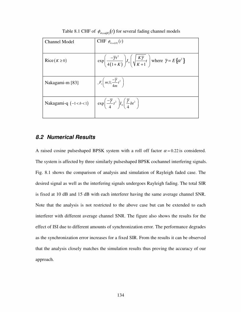
134

Table 8.1 CHF of φα cos θ( ) t( ) for several fading channel models

Channel Model CHF ( ) ( )costα θφ

Rice ( )0K ≥ ( )

2

0exp4 1 1

t KJ t

K K

γ γ−+ +

where γ = E α 2

Nakagami-m [83] 21 1 ;1;

4F m t

m

γ−

Nakagami-q ( )1 1b− < < 2 20exp

4 4t I bt

γ γ−

8.2 Numerical Results

A raised cosine pulseshaped BPSK system with a roll off factor 0.22α = is considered.

The system is affected by three similarly pulseshaped BPSK cochannel interfering signals.

Fig. 8.1 shows the comparison of analysis and simulation of Rayleigh faded case. The

desired signal as well as the interfering signals undergoes Rayleigh fading. The total SIR

is fixed at 10 dB and 15 dB with each interferer having the same average channel SNR.

Note that the analysis is not restricted to the above case but can be extended to each

interferer with different average channel SNR. The figure also shows the results for the

effect of ISI due to different amounts of synchronization error. The performance degrades

as the synchronization error increases for a fixed SIR. From the results it can be observed

that the analysis closely matches the simulation results thus proving the accuracy of our

approach.

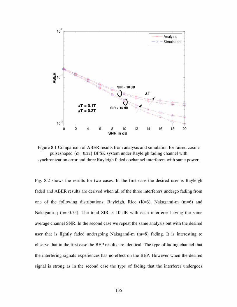
135

0 2 4 6 8 10 12 14 16 18 2010

-2

10-1

100

AnalysisSimulation

∆∆∆∆T = 0.1T∆∆∆∆T = 0.3T

∆∆∆∆T

AB

ER

SNR in dB

SIR = 10 dB

SIR = 15 dB

Figure 8.1 Comparison of ABER results from analysis and simulation for raised cosine pulseshaped ( )0.22α = BPSK system under Rayleigh fading channel with

synchronization error and three Rayleigh faded cochannel interferers with same power.

Fig. 8.2 shows the results for two cases. In the first case the desired user is Rayleigh

faded and ABER results are derived when all of the three interferers undergo fading from

one of the following distributions; Rayleigh, Rice (K=3), Nakagami-m (m=6) and

Nakagami-q (b= 0.75). The total SIR is 10 dB with each interferer having the same

average channel SNR. In the second case we repeat the same analysis but with the desired

user that is lightly faded undergoing Nakagami-m (m=8) fading. It is interesting to

observe that in the first case the BEP results are identical. The type of fading channel that

the interfering signals experiences has no effect on the BEP. However when the desired

signal is strong as in the second case the type of fading that the interferer undergoes

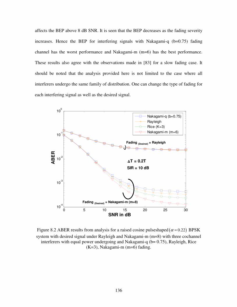
136

affects the BEP above 8 dB SNR. It is seen that the BEP decreases as the fading severity

increases. Hence the BEP for interfering signals with Nakagami-q (b=0.75) fading

channel has the worst performance and Nakagami-m (m=6) has the best performance.

These results also agree with the observations made in [83] for a slow fading case. It

should be noted that the analysis provided here is not limited to the case where all

interferers undergo the same family of distribution. One can change the type of fading for

each interfering signal as well as the desired signal.

0 5 10 15 20 25 3010

-4

10-3

10-2

10-1

100

Nakagami-q (b=0.75)RayleighRice (K=3)Nakagami-m (m=6)

∆∆∆∆T = 0.2TAB

ER

SNR in dB

SIR = 10 dB

Fading (Desired) = Nakagami-m (m=8)

Fading (Desired) = Rayleigh

Figure 8.2 ABER results from analysis for a raised cosine pulseshaped ( )0.22α = BPSK system with desired signal under Rayleigh and Nakagami-m (m=8) with three cochannel

interferers with equal power undergoing and Nakagami-q (b= 0.75), Rayleigh, Rice (K=3), Nakagami-m (m=6) fading.

137

8.3 Conclusions

Analysis for computing the precise BEP for a bandlimited BPSK system with

bandlimited CCI was presented. The analysis is applicable to signals under generalized

fading channels under non identical conditions even when the each received signal

undergoes different fading.

138

Chapter 9

9 Conclusions and Future Work

In recent years the idea of using cooperation among wireless nodes to improve end-to-

end performance of wireless communication has gained tremendous attention.

Information theoretic analyses have shown the potential for cooperative communications

to achieve higher capacity than traditional point-to-point serial multi-hop communication.

In our research we have tried to investigate the performance of cooperative

communication under more practical conditions. In the following sections we first

summarize the research performed in this dissertation and then discuss some interesting

questions that may be followed up as future work in the area.

9.1 Summary of dissertation work

In chapter 2 we presented a computationally efficient method to compute ergodic and

outage capacities for distributed OSTBC communication scheme where links may

undergo non-identical fading channels. Chapter 3 investigated the impact of time

synchronization errors on the end-to-end ABER performance for bandlimited cooperative

transmission under different fading channels. It was found that under certain channel

conditions where high diversity gains are achievable distributed OSTBC under timing

error can perform better than a perfectly synchronized SISO system. Chapter 4 explored

the relationship between node participation in cooperation and range. It was shown that

increasing the number of nodes participating in cooperation under randomized STBC

scheme does not increase the range in a linear fashion. It reaches a limit beyond which

139

range cannot be improved significantly. In chapter 5 we described a selective decode and

forward (SDF) protocol and investigated the effect of imperfect regeneration at the relay

on the end-to-end ABER performance. We presented a framework that can be used to

analyze the combined effect of propagation, geometry and forwarding criterion. It was

found that placement of relay near the source improves cooperative diversity

performance compared to the case when the relay is near the destination. This is an

important result because relays can now be chosen based on their position location aiding

clustering criteria for cooperation. It was also shown that choosing a higher SNR

threshold from a range of values that provides minimum ABER performance also

improves network capacity in terms of bits per channel used. Chapter 6 showed a log-

likelihood ratio (LLR) based criterion for SDF scheme that can achieve performance

comparable to optimum decode and forward protocol at a much lower implementation

complexity. In chapter 7 we explored the possibility of a real world application of

cooperative communication, where unmanned aerial vehicles (UAVs) equipped with

single antennas cooperate to improve performance of ground based ad-hoc networks.

Both cooperative STBC and distributed beamforming algorithms were simulated to find

the effects of implementation impairments on performance using parameters selected

form air-to-ground channel measurements. In chapter 8 the method used in chapter 3 for

analyzing the effect of timing error on cooperative communication was applied to analyze

a simple narrowband bandlimited communications system with timing error and also

affected by asynchronous bandlimited cochannel interferers under non-identical fading

channels.

140

Although we have tried to investigate a few issues related to cooperative communications,

there are many more questions that will need to be answered before the idea can be taken

from concept to reality. Some of these questions that may form the basis of future

investigations are briefly discussed in the next section.

9.2 Future work

Topics relevant to cooperative communication that may be explored in future are listed

below:

1. In chapter 3 and 4 we analyzed the impact of time synchronization errors on

cooperative relaying that use space-time codes for long haul communication.

Achieving symbol-level timing synchronization and orthogonal channel allocation

can be expensive in terms of signaling overhead required in ad-hoc networks.

Hence it is important to explore other ways and means to achieve cooperative

diversity under asynchronous modes of operation. In certain scenarios for

example in sensor networks where the destination can be equipped with greater

processing power it may be possible to accommodate a more complex receiver.

One of the ideas pursued in [125] by Valenti et al used delay diversity and

decision feedback equalizer at the destination receiver to achieve asynchronous

cooperative diversity. Another way might be to design pseudo-random codes

instead of orthogonal codes along with adaptive linear combining and iterative

decoding at the destination as suggested in [126] and [127] for spread spectrum

CDMA systems. Such a design could potentially achieve some performance

improvements in a relay system, without the need for precise frequency or timing

141

control between transceivers in the network. The author would like to

acknowledge Dr. Brian Agee for suggesting the above idea.

2. Chapter 5 discussed the SDF scheme for a simple three-node network. Scaling the

analysis to a network with more than three nodes does not appear to be easy.

Multiple relay nodes mean each relay node can independently decode and forward

information to the destination. It becomes non-trivial to characterize the effect of

imperfect transmission at the destination as the number of relay nodes that decode

incorrectly may not known a-priori. The effect of geometry may also be difficult

to analyze when the number of relay nodes are more than one. However it may be

an interesting exercise to characterize the worst case performance for a case with

multiple relay nodes under a particular distribution of relay nodes that may be of

practical interest.

3. The fundamental idea behind cooperative communication is to exploit the

broadcast nature of the wireless medium. The source node broadcasts to the relay

nodes and each relay transmits all of this information to the destination where the

destination takes advantage of the inherent spatial diversity to improve

performance. However it is obvious that as the number of relay nodes increase the

amount of redundant information transmitted from the relays to the destination

becomes high. There may be a point beyond which this redundancy results in

diminishing returns in terms of energy efficiency. A recent breakthrough in signal

processing area termed “compressive sampling” suggests an alternate theory to

Nyquist theorem [128]. The central idea in compressive sampling is that the

number of samples needed to capture a signal depends primarily on its structural

142

content, rather than its bandwidth. By using nonlinear recovery algorithms, it is

shown that signals can be reconstructed from highly incomplete data.

Compressive sampling shows how data compression can be implicitly

incorporated into the data acquisition process. This idea may be applied to the

broadcast phase of cooperative communication where the relays can be viewed as

data acquisition units in a compressive sampling process [129]. This data which is

then relayed to the destination can be recovered at the destination using the non-

linear recovery techniques. This scheme may also hold the potential for reducing

the total bandwidth and hardware required by the system. Exploring new

protocols and recovery algorithms for the above scheme and analyzing the

performance can be an interesting problem that can be pursued in future.

4. In chapter 5 we described the exact end-to-end ABER performance and energy

efficiency of a selective decode and forward (SDF) cooperative communication

scheme. We were able to analyze the system as the system could be reduced to an

equivalent symbol by symbol relaying system. However most of today’s wireless

ad-hoc networks are designed to be packet based. For example in TCP-IP based

network, the physical layer incorporates channel coding and the transport layer

uses retransmissions to ensure reliability. Channel coding ensures that the packet

drops are small but at the same time powerful coding techniques can also take

away bandwidth efficiency. Packet retransmissions in the absence of strong

channel codes can result in huge delays and use up more resources. This tradeoff

becomes even more important in a cooperative communication network. Packet

drops among cooperating nodes can severely degrade the system in terms of delay.

143

The cooperating nodes may also drop or receive different packets from the source

resulting in different acknowledgement packets resulting in more traffic and use

of more resources. On the other hand design of channel codes for worst case

scenario may also be detrimental as packets may still be dropped due to different

queues at different nodes causing more severe delays. Hence a fundamental

tradeoff between coding and retransmission needs to be understood before a

cross-layer based approach can be applied to packet based implementation of

cooperative communication.

5. Global positioning systems (GPS) based technology is expected to get smaller,

cheaper and more accurate in the future [69]. This allows for better timing control

for node level transmission and network synchronization. Better knowledge about

position location of neighboring nodes can also help in clustering of nodes for

cooperation. In order to take advantage of these benefits of GPS technology and

to ascertain the improvement in performance and tradeoff with implementation

complexity of different cooperative communication protocols it may be necessary

to build a real-time test bed for experimental evaluation and verification.

144

10 Bibliography

[1] T. S. Rappaport, A. Annamalai, R. M. Buehrer and W. H. Tranter, “Wireless Communications: Past Events and a Future Perspective” IEEE Communications Magazine, 50th Anniversary Commemorative Issue, pp.148-161, May 2002.

[2] R. Ramanathan and J. Redi, “A Brief Overview of Ad Hoc Networks: Challenges and Directions,” IEEECommunications Magazine, pp. 20-22, May 2002.

[3] I.F. Akyildiz, Xudong Wang, “A survey on wireless mesh networks,” IEEE Communications Magazine, Vol. 43, pp. S23 - S30, Sept. 2005.

[4] I.F. Akyildiz, Weilian Su, Y. Sankarasubramaniam, E. Cayirci, “A survey on sensor networks,” IEEE Communications Magazine, Vol. 40, pp.102 – 114, Aug. 2002.

[5] A.J. Goldsmith, S.B. Wicker, “Design challenges for energy-constrained ad hoc wireless networks,” IEEE Wireless Communications, Vol. 9, pp. 8 – 27, Aug. 2002.

[6] G. Pottie and W. Kaiser, “Wireless Integrated Network Sensors,” Communications of the ACMß, vol. 43, no.5, pp. 51-58, May 2000.

[7] D. Estrin, Embedded, Everywhere - A Research Agenda for Networked Systems of Embedded Computers, Editor, National Academy Press, Washington D.C., 2001.

[8] J. M. Kahn, R. H. Katz and K. Pister, “Next Century Challenge: Mobile Networking for Smart Dust,” Proc. ACM MOBICOM, Seattle, pp. 271-278, Aug. 1999.

[9] Daniel Aguayo, John Bicket, Sanjit Biswas, Glenn Judd, Robert Morris, Link-level Measurements from an 802.11b Mesh Network, SIGCOMM 2004, Aug 2004.

[10] V. Kawadia, P.R.Kumar, "Experimental Investigations into TCP Performance over Wireless Multihop Networks," ACM SIGCOMM 2005, Workshop on experimental approaches to wireless network design and analysis, Aug 22, 2005.

[11] M. Haenggi, D. Puccinelli, “Routing in ad hoc networks: a case for long hops,” IEEE Communications Magazine,Vol. 43, pp. 93 – 101, Oct 2005.

[12] M. Shafi, D. Gesbert, Da-shan Shiu; P.J. Smith, W.H. Tranter, “Guest editorial: MIMO systems and applications. 1,” IEEE Journal on Selected Areas in Communications, vol. 21, pp. 277 – 280, April 2003.

[13] M. Shafi, D. Gesbert, Da-shan Shiu; P.J. Smith, W.H. Tranter, “Guest editorial MIMO systems and applications. II,” IEEE Journal on Selected Areas in Communications, vol. 21, pp. 681 – 683, June 2003.

[14] E. C. van der Meulen, “Three-terminal communication channels,” Adv. Appl. Probab., vol. 3, pp. 120–154, 1971.

[15] T. M. Cover and A. A. El Gamal, “Capacity Theorems for the Relay Channel,” IEEE Trans. Inform. Theory, vol. 25, pp. 572–584, Sept. 1979.

[16] G. Kramer and A. J. van Wijngaarden, “On the White Gaussian Multiple-Access Relay Channel,” Proc. IEEE Int. Symp.Information Theory (ISIT), (Sorrento, Italy), p. 40, June 2000.

145

[17] M. Gastpar, G. Kramer, and P. Gupta, “The Multiple-Relay Channel: Coding and Antenna-Clustering Capacity,” Proc. IEEE Int. Symp. Information Theory (ISIT), p. 136, July 2002.

[18] P. Gupta and P. R. Kumar, “Towards an Information Theory of Large Networks: An Achievable Rate Region,” IEEE Trans. Inform. Theory, vol. 49, pp. 1877–1894, Aug. 2003.

[19] M. Khojastepour, A. Sabharwal, and B. Aazhang, “On capacity of Gaussian ‘cheap’ relay channel,” IEEE GLOBECOMM, pp. 1776–1780, Dec. 2003.

[20] J. Nicholas Laneman, “Cooperative Diversity in Wireless Networks: Algorithms and Architectures”, PhD dissertation, September 2002.

[21] J.N. Laneman, G.W. Wornell, “Distributed space-time-coded protocols for exploiting cooperative diversity in wireless networks,” IEEE Trans. Inform. Theory, vol. 49, pp. 2415 – 2425 Oct. 2003.

[22] J.N. Laneman, D.N.C. Tse, G.W. Wornell, “Cooperative Diversity in Wireless Networks: Efficient Protocols and Outage Behavior,” IEEE Trans., Inform. Theory, vol. 50, pp.3062 – 3080, Dec. 2004.

[23] A. Sendonaris, E. Erkip, B. Aazhang, “User cooperation diversity: Part I. System description” IEEE Trans. on Commun., vol. 51, pp. 1927 – 1938, Nov. 2003.

[24] A. Sendonaris, E. Erkip, B. Aazhang, “User cooperation diversity: Part II. Implementation aspects and performance Analysis,” IEEE Trans. on Commun., vol. 51, pp.1939 – 1948, Nov. 2003.

[25] A. Stefanov and E. Erkip, “On the Performance Analysis of Cooperative Space-Time Systems,” IEEE WCNC, pp. 729–34, March 2003.

[26] A. Stefanov, E. Erkip, “Cooperative coding for wireless networks,” IEEE Trans. Commun., vol. 52, pp. 1470 – 1476, Sept. 2004.

[27] Zinan Lin, E. Erkip, M. Ghosh, “Adaptive modulation for coded cooperative systems,” IEEE SPAWC, pp. 615 – 619, June 2005.

[28] D. Gunduz, E. Erkip, “Source and channel coding for cooperative relaying,” IEEE SPAWC, pp. 950 – 954, June 2005.

[29] T. E. Hunter A. Nosratinia, “Distributed Protocols for User Cooperation in Multi-User Wireless Networks,” IEEE GLOBECOMM, vol 6, pp. 3788-3792, Dec 2004.

[30] M. Janani, A. Hedayat, T.E. Hunter, A. Nosratinia, “Coded Cooperation in Wireless Communications: Space-Time Transmission and Iterative Decoding,” IEEE Trans. Sig. Proc., vol. 52, no. 2, pp. 362–71, Feb. 2004.

[31] M. Katz and S. Shamai (Shitz), “Communicating to co-located ad-hoc receiving nodes in a fading environment,” Proc. ISIT, p. 115, Jul. 2004.

[32] R. Pabst, B.H. Walke, D.C. Schultz, P. Herhold, H. Yanikomeroglu, S. Mukherjee, H. Viswanathan, M. Lott, W. Zirwas, M. Dohler, H. Aghvami, D.D. Falconer, G.P. Fettweis, “Relay-based deployment concepts for wireless and mobile broadband radio,” IEEE Comm. Magazine, vol. 42, pp. 80 – 89, Sept. 2004.

146

[33] E. Zimmermann, P. Herhold, and G. Fettweis, “On the Performance of Cooperative Diversity Protocols in Practical Wireless Systems,” IEEE VTC, vol.4, pp. 2212 – 2216, Oct. 2003.

[34] Shuguang Cui; A.J. Goldsmith, A. Bahai, “Energy-efficiency of MIMO and cooperative MIMO techniques in sensor networks,” IEEE Journal on Selected Areas in Comm., vol. 22, pp.1089 – 1098, Aug. 2004.

[35] M.O. Hasna, M.-S. Alouini, “Outage probability of multihop transmission over Nakagami fading channels,” IEEE Commun. Letters, vol. 7, pp. 216 – 218, May 2003.

[36] M.O. Hasna, M.-S. Alouini, “End-to-end performance of transmission systems with relays over Rayleigh-fading channels,” IEEE Trans. Wireless Comm., vol. 2, pp.1126 – 1131, Nov. 2003.

[37] M.O. Hasna, M.-S. Alouini, “Harmonic mean and end-to-end performance of transmission systems with relays,” IEEE Trans. Commun., vol. 52, pp.130 – 135, Jan. 2004.

[38] M. Dohler, H. Aghvami, “Information outage probability of distributed STBCs over Nakagami fading channels,” IEEE Commun. Letters, vol. 8, pp. 437 – 439, July 2004.

[39] P.A. Anghel, M. Kaveh, “Exact symbol error probability of a Cooperative network in a Rayleigh-fading environment,” IEEE Trans. Wireless Commun., vol. 3, pp.1416 – 1421 Sept. 2004.

[40] P.A. Anghel, M. Kaveh, “On the diversity of cooperative systems,” Proc. ICASSP, vol. 4, pp. iv-577 - iv-580, May 2004.

[41] A. Ribeiro, Xiaodong Cai, G.B. Giannakis, “Symbol error probabilities for general Cooperative links,” IEEE Trans. on Wireless Commun., vol. 4, pp. 1264 – 1273, May 2005.

[42] Y. Yu, A. Ribeiro, N.D. Sidiropoulos, G.B. Giannakis, “Cooperative random access with long PN spreading codes,” Proc. IEEE ICASSP, vol. 3, pp. iii/517 - iii/520, March 2005.

[43] Y.W. Hong, A. Scaglione, “Energy-Efficient Broadcasting with Cooperative Transmission in Wireless Sensory Ad Hoc Networks,” Proc. Allerton, Oct. 2003.

[44] Y.-W. Hong, A. Scaglione, ”Cooperative Transmission in Wireless Multi-hop Ad hoc Networks using Opportunistic Large Arrays,” IEEE SPAWC, pp. 120 – 124, June 2003.

[45] A. Scaglione, Y.-W. Hong, ”Opportunistic Large Arrays: Cooperative transmission in wireless multihop adhoc networks to reach far distances,” IEEE Trans. on Signal Proc., vol. 51, No. 8, Aug. 2003.

[46] B. Sirkeci-Mergen, A. Scaglione, “Signal acquisition for cooperative transmissions in multi-hop ad-hoc networks,” IEEE ICASSP, vol. 2, pp. ii - 345-8, May 2004.

[47] B. Sirkeci-Mergen, A. Scaglione, “Coverage analysis of cooperative broadcast in wireless networks,” IEEE SPAWC, pp. 16 – 20, July 2004.

[48] Yao-Win Hong, A. Scaglione, “A scalable synchronization protocol for large scale sensor networks and its application,” IEEE Journal on Selected Areas in Commun., vol. 23, pp. 1085 – 1099, May 2005.

147

[49] B. Sirkeci-Mergen, A. Scaglione, “Randomized distributed space-time coding for cooperative communication in self organized networks,” IEEE SPAWC, pp. 500 – 504, June 2005.

[50] T. Miyano, H. Murata, K. Araki, “Cooperative Relaying Scheme with Space Time Code for Multihop Communications among Single Antenna Terminals” Globecomm 2004.

[51] P. Tarasak, H. Minn, V. K. Bhargava, “Differential Modulation for Two-User Cooperative Diversity Systems” Globecomm 2004.

[52] I. Hammerstroem, M. Kuhn, B. Rankov, A. Wittneben, “Space-time processing for cooperative relay networks,” IEEE VTC, vol. 1, pp. 404 – 408, Oct. 2003.

[53] I. Hammerstroem, M. Kuhn, A. Wittneben, “Cooperative diversity by relay phase rotations in block fading environments,” IEEE SPAWC, pp. 293 – 297, July 2004.

[54] I. Hammerstroem, M. Kuhn, A. Wittneben, “Impact of relay gain allocation on the performance of cooperative diversity networks,” IEEE VTC, vol. 3, pp. 1815 – 1819, Sept. 2004.

[55] B. Rankov, A. Wittneben, “Distributed spatial multiplexing in a wireless network Signals,” Proc. Asilomar, vol. 2, pp.1932 – 1937, Nov. 2004.

[56] B. Rankov, A. Wittneben, “On the capacity of relay-assisted wireless MIMO channels,” IEEE SPAWC, pp. 323 – 327, July 2004.

[57] A. Wittneben, I. Hammerstroem, M. Kuhn, “Joint cooperative diversity and scheduling in low mobility wireless networks” IEEE GLOBECOM, vol. 2, pp. 780 – 784, Nov. 2004

[58] A. Wittneben, I. Hammerstroem, “Multiuser zero forcing relaying with noisy channel state information,” IEEE WCNC, vol. 2, pp. 1018 – 1023, March 2005.

[59] S. Barbarossa, F. Bucciarelli, “On the connectivity of cooperative and non cooperative wireless communication networks,” IEEE SPAWC, pp. 905 – 909, June 2005.

[60] G. Scutari, S. Barbarossa, “Distributed space-time coding for regenerative relays,” Proc. IEEE Trans. Wireless Commun., vol. 4, pp. 2387-2399, Sept. 2005.

[61] J. Mietzner, R. Thobaben, P.A. Hoeher, “Analysis of the expected error performance of cooperative wireless networks employing distributed space-time codes,” IEEE GLOBECOM, vol. 5, pp. 2854 – 2858, Nov 2004.

[62] G. Barriac, R. Mudumbai, U. Madhow, “Distributed beamforming for information transfer in sensor networks,” Third Int. Symp. on Information Processing in Sensor Networks, 2004. pp.81 – 88, Apr. 2004.

[63] R. Mudumbai, J. Hespanha, U. Madhow, G. Barriac, “Scalable feedback control for distributed beamforming in sensor networks,” Proc. IEEE ISIT, pp. 137 – 141, Sept. 2005.

[64] H. Ochiai, P. Mitran, H.V. Poor, V. Tarokh, “Collaborative Beamforming for Distributed Wireless Ad Hoc Sensor Networks,” IEEE Trans. on Sig. Proc., vol. 53, pp. 4110 – 4124, Nov. 2005.

[65] P. Mitran, H. Ochiai, V. Tarokh, “Space-time diversity enhancements using collaborative communications,” IEEE Trans. on Inform. Theory, vol. 51, pp. 2041 – 2057, June 2005.

148

[66] R.U. Nabar, F. W. Kneubuhler, H. Bolcskei, “Performance limits of amplify-and-forward based fading relay channels,” IEEE Proc. ICASSP, vol. 4, pp. iv-565 - iv-568, May 2004.

[67] R.U. Nabar, H. Bolcskei, F. W. Kneubuhler, “Fading relay channels: performance limits and space-time signal design,” IEEE Journal Selected Areas in Commun., vol. 22, pp. 1099 – 1109, Aug. 2004 .

[68] V.I. Morgenshtern, H. Bolcskei, R.U. Nabar, “Distributed orthogonalization in large interference relay networks,” IEEE Proc. ISIT, pp. 1211 – 1215, Sept. 2005.

[69] S. Knappe, L. Liew, V. Shah, P. Schwindt, J. Moreland, L. Hollberg and J. Kitching, "A microfabricated atomic clock," Appl. Phys. Lett.85, 1460, 2004.

[70] G. J. Foschini and M. J. Gans, “On limits of wireless communications in a fading environment when using multiple antennas,” Wireless Personal Commun., vol. 6, pp. 311–335, 1998.

[71] S. M. Alamouti, “A simple transmit diversity technique for wireless communications,” IEEE J. Select. Areas Commun., vol. 16, no. 8, Oct. 1998.

[72] V. Tarokh, N. Seshadri, and A.R. Calderbank, “Space-time codes for high data rate wireless communication: performance criterion and code construction,” IEEE Trans. Information Theory, vol. 44, pp. 744 – 765, 1998.

[73] J. Abate, P. P. Valkó, “Multi-precision Laplace transform inversion,” International Journal for Numerical Methods in Engineering, vol. 60, no. 5, pp. 979-993, May 2004.

[74] V. Tarokh, H. Jafarkhani, and A.R. Calderbank, “Space-time block codes from orthogonal designs,” IEEE Trans. Inf. Theory, vol. 45, no. 5, pp. 1456–1467, July 1999.

[75] E. G. Larsson and P. Stoica, Space-Time Block Coding for Wireless Communications

New York: Cambridge Univ. Press, 2003.

[76] J. Abate and W. Whitt, “Numerical inversion of Laplace transforms of probability distribution,” ORSA J. Computing, vol. 7, pp. 36–43, 1995.

[77] Young-Chai Ko, M.-S. Alouini, and M.K. Simon, “Outage probability of diversity systems over generalized fading channels,” IEEE Trans. Commun., vol. 48, pp.1783 – 1787, Nov. 2000

[78] K. Vanganuru, A. Annamalai, “Combined transmit and receive antenna diversity for WCDMA in multipath fading channels,” IEEE Comm. Letters, vol. 7, no. 8, pp. 352 – 354, Aug 2003.

[79] J. Cheng, C. Tellambura, N.C. Beaulieu, “Performance of digital linear modulations on Weibull slow-fading channels,” IEEE Trans. Commun, vol. 52, no.8 , pp.1265-1268,Aug. 2004.

[80] J. Vanelli, N. Shehadeh, “Computation of Bit-Error Probability Using the Trapezoidal Integration Rule,” IEEE Trans. on Commun., vol. 22, pp. 331 – 334, Mar 1974.

[81] Howard Ma, N. Shehadeh, J. Vanelli, “Effects of Intersymbol Interference on a Rayleigh Fast-Fading Channel,” IEEE Trans. on Commun., vol. 28, pp. 128 – 131, Jan 1980.

[82] N. C. Beaulieu and A. A. Abu-Dayya, “Bandwidth efficient QPSK in cochannel interference and fading,” IEEE Trans. Commun., vol. 43, pp. 2464-2474, Sept. 1995.

149

[83] N.C. Beaulieu, Julian Cheng, “Precise error-rate analysis of bandwidth-efficient BPSK in Nakagami fading and cochannel interference,” IEEE Trans. Commun., vol. 52, pp. 149 – 158, Jan. 2004.

[84] C. Tellambura, A. Annamalai, “Derivation of Craig's formula for Gaussian probability function,” Electronics Letters, vol. 35, pp. 1424 – 1425, Aug. 1999.

[85] A. Annamalai, C. Tellambura, V.K. Bhargava, “A general method for calculating error probabilities over fading channels,” IEEE Trans. Commun., vol. 53, pp. 841 – 852, May 2005

[86] I. S. Gradshteyn and I. M. Ryzhik, Table of Integrals, Series and Products. San Diego, CA: Academic, 1995.

[87] S. Jagannathan, H. Aghajan, A. Goldsmith, “The effect of time synchronization errors on the performance of cooperative MISO systems,” IEEE GlobeCom, pp.102 - 107, Nov 2004.

[88] Yan Mei, Yingbo Hua, A. Swami, B. Daneshrad, “Combating Synchronization Errors in Cooperative Relays,” ICASSP, vol. 3, pp. 369 – 372, Mar 2005.

[89] R. Chembil Palat, A. Annamalai, J.H.Reed, “Upper bound on bit error rate for time synchronization errors in bandlimited distributed MIMO networks,” to appear, Proc. IEEE Wireless Communications and Networking Conference, April 2006, Las Vegas

[90] A. Annamalai, C. Tellambura, V.K. Bhargava, “Equal-gain diversity receiver performance in wireless channels,” IEEE Trans. Commun., vol. 48, pp. 1732 – 1745, Oct. 2000.

[91] Chunjun Gao, A.M. Haimovich, Debang Lao, “Bit error probability for space-time block code with coherent and differential detection, ” IEEE VTC, vol. 1, pp. 410 – 414, Sept. 2002.

[92] Y.-C. Jenq, “Does a Larger Intersymbol Interference Result in a Higher Probability of Error?,” IEEE Trans. Commun., vol. 28, pp. 1771 – 1773, Sep 1980.

[93] B. Sirkeci-Mergen, A. Scaglione, “Randomized distributed space-time coding for cooperative communication in self organized networks,” IEEE SPAWC, pp. 500 – 504, June 2005.

[94] T. Brown, B. Argrow, C. Dixon, S. Doshi, R. Thekkekunnel and D. Henkel, “Ad Hoc UAV Ground Network (AUGNet),” AIAA 3rd "Unmanned Unlimited" Technical Conference, Workshop and Exhibit, Chicago, Illinois, AIAA-2004-6321, Sep. 20-23, 2004.

[95] 1st Lt. Brooke Davis, http://www.edwards.af.mil/archive/2004/2004-archive-2_x45a.html

[96] J. Painter, S. Gupta and L. Wilson, “Multipath Modeling for Aeronautical Communications,” IEEE Trans. Commun., vol. 21, pp. 658 – 662, May 1973.

[97] J. Hagenauer, F. Dolainsky, E. Lutz, W. Papke and R. Schweikert, “The maritime satellite communication channel--channel model, performance of modulation and coding,” IEEE Journal Selected Areas in Communications, vol. 5, pp. 701-713, May 1987.

[98] S.M. Elnoubi, “A simplified stochastic model for the aeronautical mobile radio channel,” IEEE 42nd Vehicular Technology Conference, vol. 2, pp. 960-963, May 1992.

[99] P. Hoeher and E. Haas, “Aeronautical channel modeling at VHF-band,” IEEE 50th Vehicular Technology Conference (VTC 1999 - Fall), vol. 4, pp. 1961-1966, Sept. 1999.

150

[100] H. Smith and J.G. Gardiner, “Wideband Characterization of the High Elevation Orbit Satellite-Mobile Channel at L-Band,” IEEE 41st Vehicular Technology Conference (VTC91), pp. 23-28, 1991.

[101] A. Jahn, H. Bischl and G. Heib, “Channel Characterisation for Spread Spectrum Satellite Communications,” IEEE 4th International Symposium on Spread Spectrum Techniques and Applications, vol. 3, pp. 1221-1226, 1996.

[102] Dyer G., Gilbert T.G., Henriksen S. and Sayadian E., “Mobile Propagation Measurements using CW and Sliding Correlator Techniques,” Antennas and Propagation International Symposium, vol. 4, pp. 1896-1899, June 1998.

[103] C. Perez-Vega and J.M. Zamanillo, “Path-loss model for broadcasting applications and outdoor communication systems in the VHF and UHF bands,” IEEE Trans. Broadcasting, vol. 8, pp. 91-96, June 2002.

[104] H. Stone, G. Clarke,“The T-Wing: A VTOL UAV for Defense and Civilian Applications,” UAV Australia Conference, Melbourne, Feb 2001.

[105] Miniature UAV’s & Future Electronic Warfare, www.aerosonde.com/downloads/Aerosonde_DSTO_EW.pdf

[106] Atmospheric Considerations for Uninhabited Aerial Vehicle (UAV) Flight Test Planning www.dfrc.nasa.gov/DTRS/1998/PDF/H-2220.pdf

[107] M.O. Hasna, M.-S. Alouini, “Optimal power allocation for relayed transmissions over Rayleigh-fading channels,” IEEE Trans. Wireless Commun., vol. 3, pp. 1999 – 2004, Nov. 2004.

[108] L. Milstein, D. Schilling, R. Pickholtz, “Comparison of Performance of 16-ary QASK and MSK Over a Frequency Selective Rician Fading Channel,” IEEE Trans. Commun., vol.29, pp. 1622- 1633, Nov 1981.

[109] X. Li, “Space-time coded multi-transmission among distributed transmitters without perfect synchronization,” IEEE Signal Process. Lett., vol. 11, pp. 948-951, Dec. 2004.

[110] D.L. Goeckel, Yonggang Hao, “Space-time coding for distributed antenna arrays,” IEEE International Conference on Communications, vol.2, pp. 747- 751, Jun 2004.

[111] Shuangqing Wei, D.L. Goeckel, M.C. Valenti, “Asynchronous cooperative diversity,” IEEE Trans. Wireless Commun., IEEE Transactions on , vol.5, pp. 1547- 1557, June 2006.

[112] T. Huang, J. Omura, L. Biederman, “Bit Error Rate Comparison of Repeater and Regenerative Communication Satellites,” IEEE Trans. Commun., vol. 28, pp. 1088 – 1097, Jul 1980.

[113] J. Adeane, M. R. D. Rodrigues, and I. J. Wassell, “Characterisation of the performance of cooperative networks in Ricean fading channels,” 12th International Conference on Telecommunications (ICT 2005), Cape Town, South Africa, May 3-6, 2005.

[114] Tairan Wang, A. Cano, G.B. Giannakis, “Efficient Demodulation in Cooperative Schemes Using Decode-and-Forward Relays,” IEEE Thirty-Ninth Asilomar Conf. on Signals, Systems and Computers, pp. 1051 – 1055, Oct. 2005.

[115] T. E. Hunter, A. Nosratinia, “Diversity through coded cooperation,” IEEE Trans. Wireless Commun. , vol.5, pp. 283- 289, Feb. 2006.

151

[116] P. Herhold, E. Zimmermann, and G. Fettweis, “A Simple Cooperative Extension to Wireless Relaying,” in International Zurich Seminar on Communications (IZS), Zurich, Switzerland, February 2004.

[117] R. Mostafa, A. Annamalai, J.H. Reed, “Performance evaluation of cellular mobile radio systems with interference nulling of dominant interferers,” IEEE Trans. on Commun., vol. 52, pp. 326 – 335, Feb. 2004.

[118] Y. Yao, X. Cai, and G. B. Giannakis, “On energy efficiency and optimum resource allocation in wireless relay transmissions,” IEEE Trans. Wireless Commun., vol. 4, pp. 2917-2927, Nov. 2005.

[119] S. Verdú, “Spectral efficiency in the wideband regime,” IEEE Trans. Inf. Theory, vol. 48, no. 6, pp. 1319–1343, Jun. 2002.

[120] S. K. Jayaweera, “A virtual MIMO-based cooperative communications architecture for energy-constrained wireless sensor networks,” IEEE Trans. Wireless Commun., vol. 5, pp. 984-989, May. 2006.

[121] Catovic, A.; Tekinay, S., “Power efficiency of user cooperation in multihop wireless networks,” IEEE Commun. Letters, vol. 9, pp. 1034- 1036, Dec. 2005.

[122] R. Madan, N.B. Mehta, A.F. Molisch, J. Zhang, “ Energy-Efficient Cooperative Relaying over Fading Channels with Simple Relay Selection,” Proc. IEEE Globecom, Nov, 2006.

[123] Weifeng Su, A.K. Sadek, K.J.R. Liu, “SER performance analysis and optimum power allocation for decode-and-forward cooperation protocol in wireless networks,” IEEE WCNC, vol. 2, pp. 984 – 989, 13-17 March 2005.

[124] Sang Wu Kim, Eun Yong Kim, “Optimum receive antenna selection minimizing error probability,” IEEE WCNC, vol. 1, pp. 441 – 447, 13-17 March 2003.

[125] Shuangqing Wei; D.L. Goeckel, M.C. Valenti, “Asynchronous cooperative diversity,” IEEE Trans. Wireless Commun., vol.5, pp. 1547- 1557, June 2006.

[126] B.G. Agee, “Solving the near-Far Problem: Exploitation of Spatial and Spectral Diversity in Wireless Personal Communication Networks,” Proc. Virginia Tech's Third Symposium on Wireless Personal Communications, Blacksburg, VA, June 9-11, 1993.

[127] U. Madhow, M.L. Honig, “On the average near-far resistance for MMSE detection of direct sequence CDMA signals with random spreading,” IEEE Trans. Information Theory, vol.45, pp.2039-2045, Sep 1999.

[128] E.J. Candes, J. Romberg, T. Tao, “Robust uncertainty principles: exact signal reconstruction from highly incomplete frequency information,” IEEE Trans. Information Theory, vol.52, pp. 489- 509, Feb. 2006.

[129] Haupt, J.; Nowak, R., “Signal reconstruction from noisy random projections,” IEEE Trans. Information Theory, vol.52, pp. 4036- 4048, Sept. 2006.

152

VITA

RAMESH CHEMBIL PALAT received his B.Tech. degree in Electronics and Communications

Engineering from University of Calicut, India in 1998 and M.S. degree in Electrical Engineering

from Virginia Tech in 2002. He expects to graduate with a PhD in Electrical Engineering from

Virginia Tech in December 2006. Before coming to Virginia Tech he worked as a software

engineer with Infosys Technologies Ltd. in 1999. During summers of 2001 and 2002, he worked

with Analog Devices Inc. and Microsoft Research respectively. He has accepted a position at

Qualcomm where he will be working on next generation Flash OFDM technology. His research

interests include cooperative communications, space-time processing, and signal processing for

software defined radios.

Documents

Performance Analysis of Cooperative Communication for Wireless