Performance Analysis of Computer Systems - tu-dresden.de fileQueuing/Kendall notation Queuing in daily life Exponential distribution and its memoryless property Little’s law Stochastic

Holger Brunst ([email protected])

Matthias S. Mueller ([email protected])

Performance Analysis of

Computer Systems

Introduction to Queuing Theory



Summary of Previous Lecture

Performance Simulation and Prediction

3

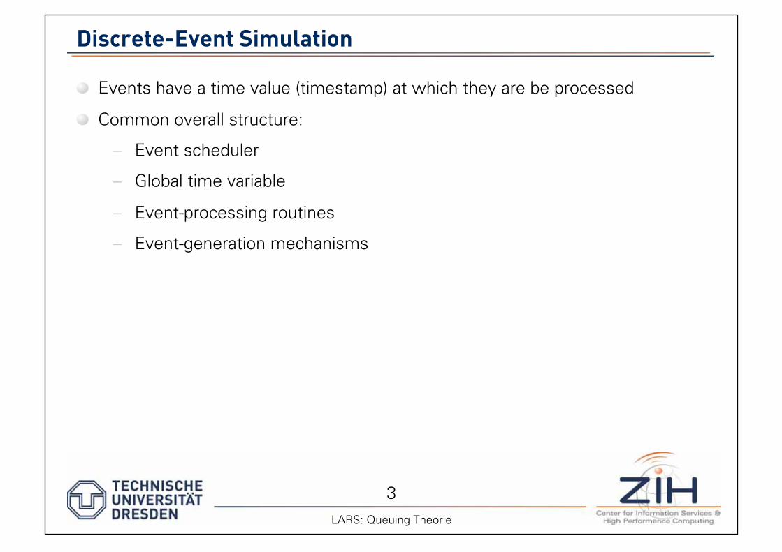
Discrete-Event Simulation

Events have a time value (timestamp) at which they are be processed

Common overall structure:

– Event scheduler

– Global time variable

– Event-processing routines

– Event-generation mechanisms

LARS: Queuing Theorie

4

Discrete-Event Simulation (cont.)

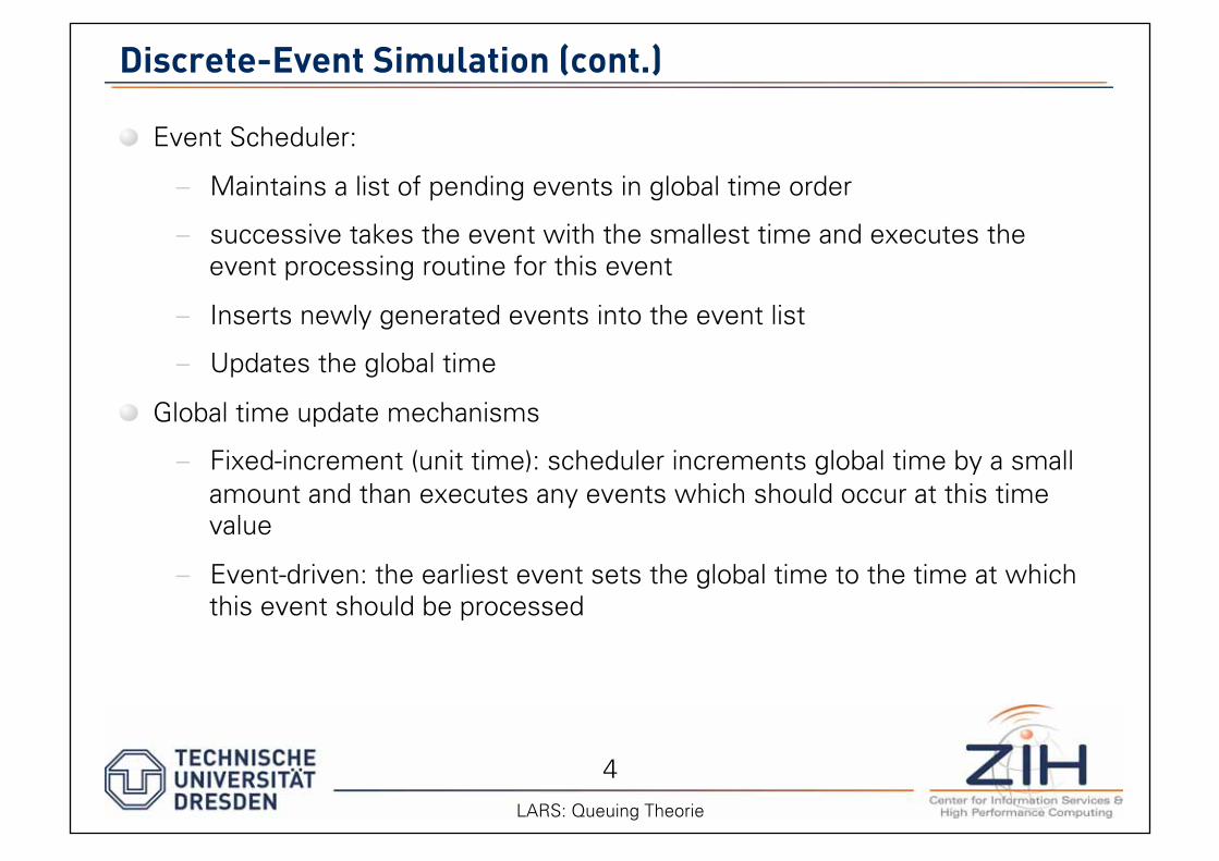
Event Scheduler:

– Maintains a list of pending events in global time order

– successive takes the event with the smallest time and executes the event processing routine for this event

– Inserts newly generated events into the event list

– Updates the global time

Global time update mechanisms

– Fixed-increment (unit time): scheduler increments global time by a small amount and than executes any events which should occur at this time value

– Event-driven: the earliest event sets the global time to the time at which this event should be processed


5

Discrete-Event Simulation (cont.)

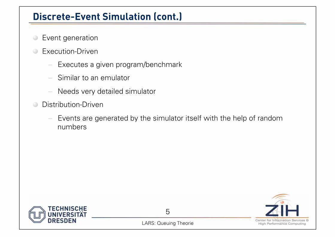
Event generation

Execution-Driven

– Executes a given program/benchmark

– Similar to an emulator

– Needs very detailed simulator

Distribution-Driven

– Events are generated by the simulator itself with the help of random numbers


6

Parallel Discrete-Event Simulation

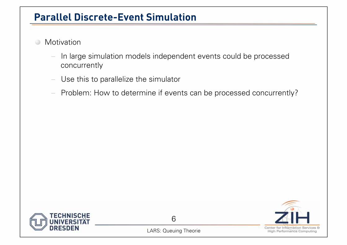
Motivation

– In large simulation models independent events could be processed concurrently

– Use this to parallelize the simulator

– Problem: How to determine if events can be processed concurrently?


7

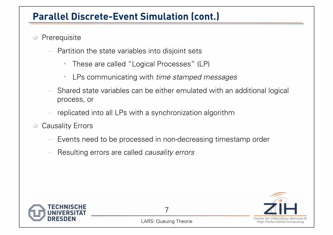
Parallel Discrete-Event Simulation (cont.)

Prerequisite

– Partition the state variables into disjoint sets

• These are called “Logical Processes” (LP)

• LPs communicating with time stamped messages

– Shared state variables can be either emulated with an additional logical process, or

– replicated into all LPs with a synchronization algorithm

Causality Errors

– Events need to be processed in non-decreasing timestamp order

– Resulting errors are called causality errors


8

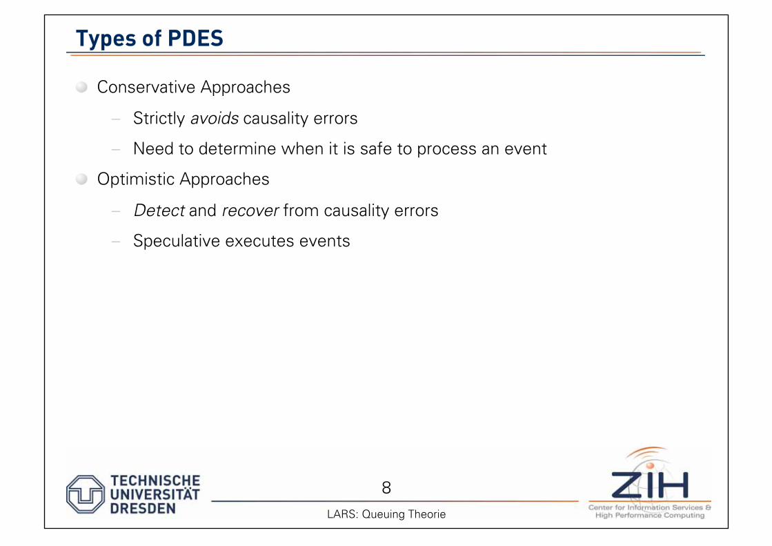
Types of PDES

Conservative Approaches

– Strictly avoids causality errors

– Need to determine when it is safe to process an event

Optimistic Approaches

– Detect and recover from causality errors

– Speculative executes events




Introduction to Queuing Theory

10 LARS: Queuing Theorie

Introduction to Queuing Models

If the facts don’t fit the theory, change the facts.

Albert Einstein


Outline

Motivation

Queuing/Kendall notation

Queuing in daily life

Exponential distribution and its memoryless property

Little’s law

Stochastic processes, birth-death process

M|M|1 queuing model


Motivation

Sharing of system resources in computer systems:

– CPU, Disk, Network, etc.

Generally, only one job can use the resource at any time

All other jobs using the same resource wait in queues

Queuing or queuing theory helps in determining the time that jobs spend in various system queues.

These times can be combined to predict the response time of jobs


Queuing Notation

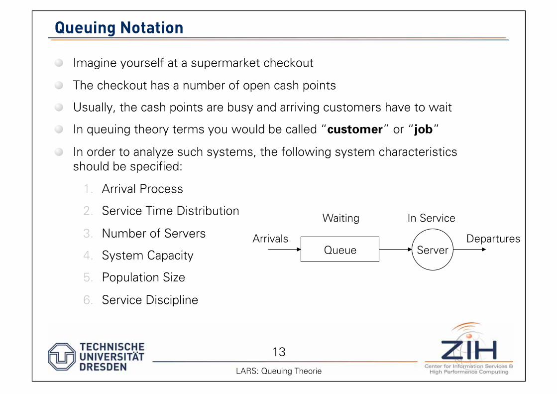
Imagine yourself at a supermarket checkout

The checkout has a number of open cash points

Usually, the cash points are busy and arriving customers have to wait

In queuing theory terms you would be called “customer” or “job”

In order to analyze such systems, the following system characteristics should be specified:

1. Arrival Process

2. Service Time Distribution

3. Number of Servers

4. System Capacity

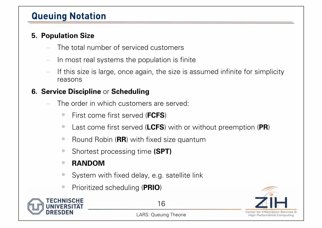
5. Population Size

6. Service Discipline

Queue Server Arrivals

Waiting

Departures

In Service


Queuing Notation

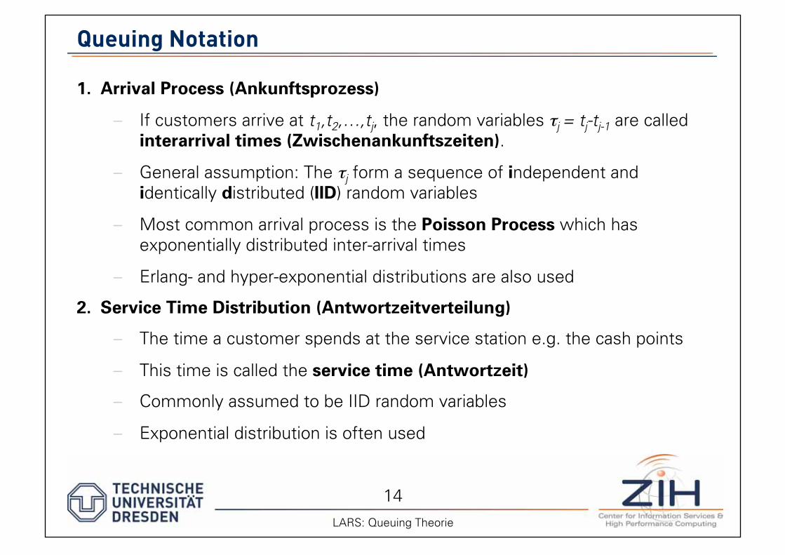
1. Arrival Process (Ankunftsprozess)

– If customers arrive at t1,t2,…,tj, the random variables j = tj-tj-1 are called interarrival times (Zwischenankunftszeiten).

– General assumption: The j form a sequence of independent and identically distributed (IID) random variables

– Most common arrival process is the Poisson Process which has exponentially distributed inter-arrival times

– Erlang- and hyper-exponential distributions are also used

2. Service Time Distribution (Antwortzeitverteilung)

– The time a customer spends at the service station e.g. the cash points

– This time is called the service time (Antwortzeit)

– Commonly assumed to be IID random variables

– Exponential distribution is often used


Queuing Notation

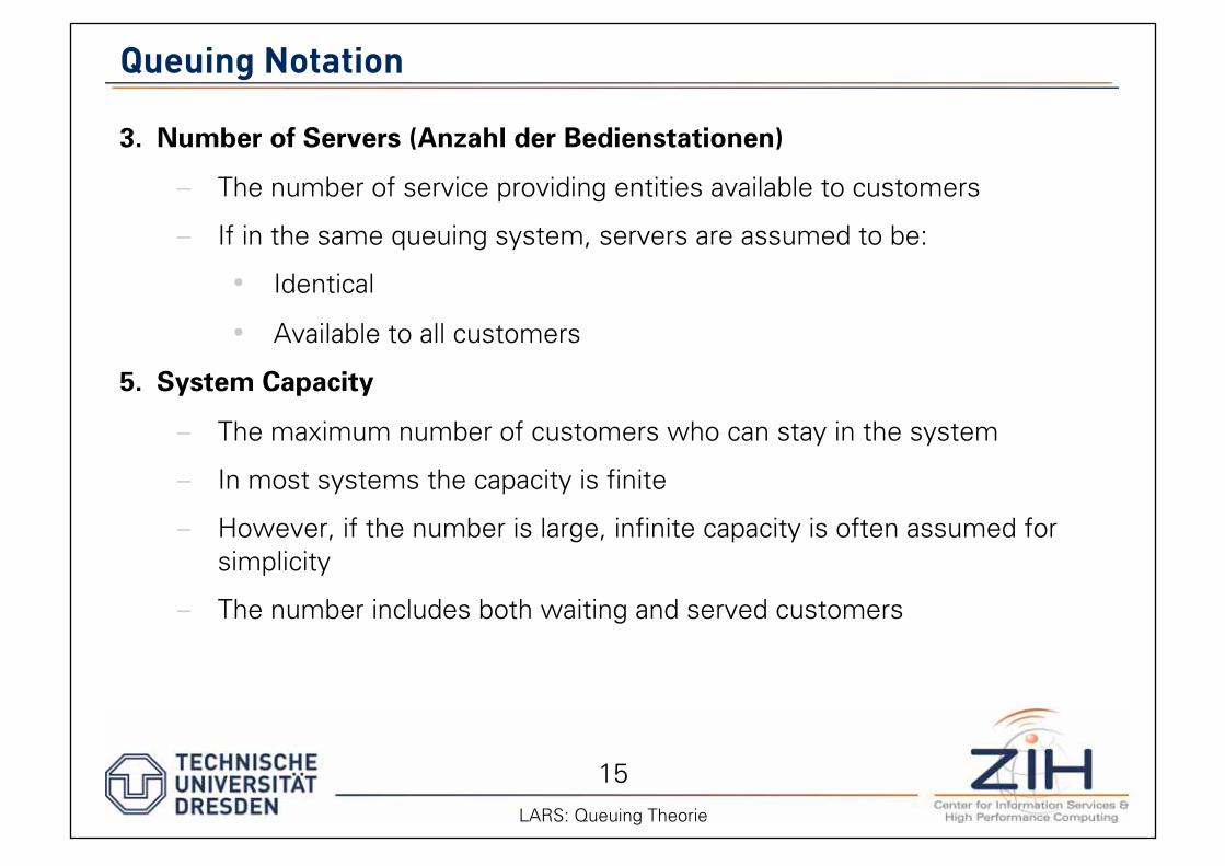
3. Number of Servers (Anzahl der Bedienstationen)

– The number of service providing entities available to customers

– If in the same queuing system, servers are assumed to be:

• Identical

• Available to all customers

5. System Capacity

– The maximum number of customers who can stay in the system

– In most systems the capacity is finite

– However, if the number is large, infinite capacity is often assumed for simplicity

– The number includes both waiting and served customers


Queuing Notation

5. Population Size

– The total number of serviced customers

– In most real systems the population is finite

– If this size is large, once again, the size is assumed infinite for simplicity reasons

6. Service Discipline or Scheduling

– The order in which customers are served:

• First come first served (FCFS)

• Last come first served (LCFS) with or without preemption (PR)

• Round Robin (RR) with fixed size quantum

• Shortest processing time (SPT)

• RANDOM

• System with fixed delay, e.g. satellite link

• Prioritized scheduling (PRIO)


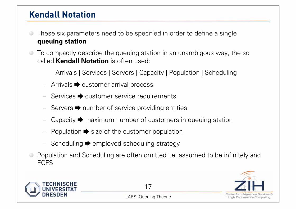
Kendall Notation

These six parameters need to be specified in order to define a single queuing station

To compactly describe the queuing station in an unambigous way, the so called Kendall Notation is often used:

Arrivals | Services | Servers | Capacity | Population | Scheduling

– Arrivals customer arrival process

– Services customer service requirements

– Servers number of service providing entities

– Capacity maximum number of customers in queuing station

– Population size of the customer population

– Scheduling employed scheduling strategy

Population and Scheduling are often omitted i.e. assumed to be infinitely and FCFS


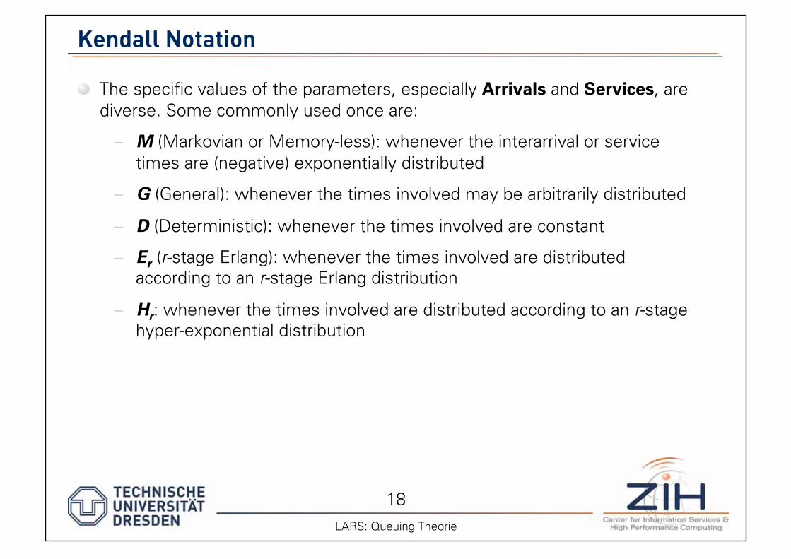
Kendall Notation

The specific values of the parameters, especially Arrivals and Services, are diverse. Some commonly used once are:

– M (Markovian or Memory-less): whenever the interarrival or service times are (negative) exponentially distributed

– G (General): whenever the times involved may be arbitrarily distributed

– D (Deterministic): whenever the times involved are constant

– Er (r-stage Erlang): whenever the times involved are distributed according to an r-stage Erlang distribution

– Hr: whenever the times involved are distributed according to an r-stage hyper-exponential distribution


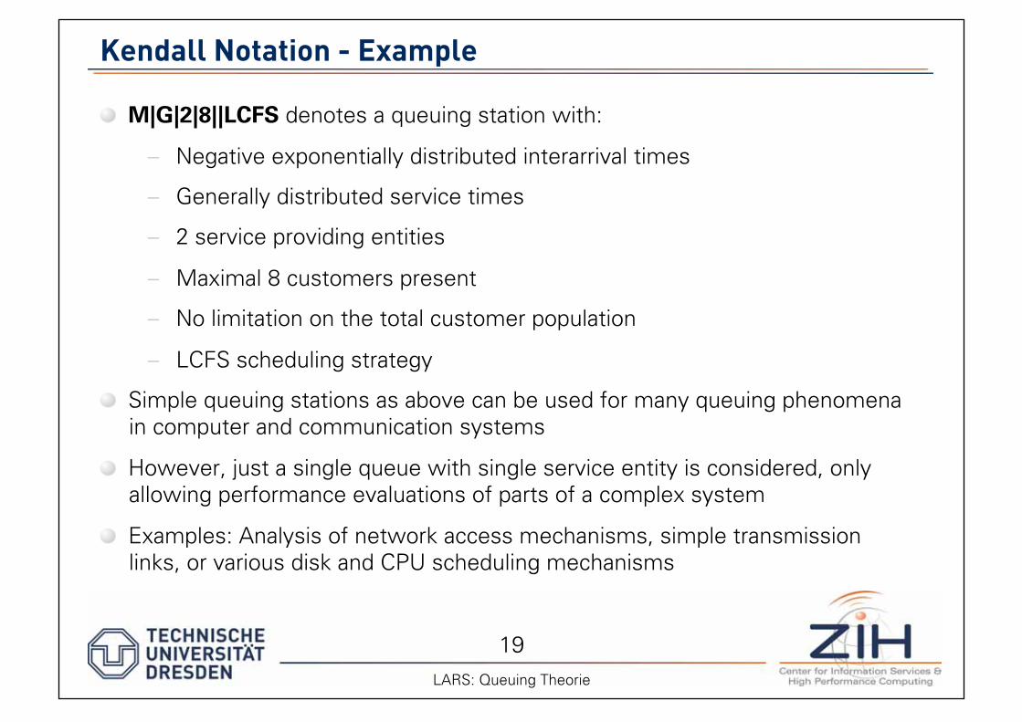
Kendall Notation - Example

M|G|2|8||LCFS denotes a queuing station with:

– Negative exponentially distributed interarrival times

– Generally distributed service times

– 2 service providing entities

– Maximal 8 customers present

– No limitation on the total customer population

– LCFS scheduling strategy

Simple queuing stations as above can be used for many queuing phenomena in computer and communication systems

However, just a single queue with single service entity is considered, only allowing performance evaluations of parts of a complex system

Examples: Analysis of network access mechanisms, simple transmission links, or various disk and CPU scheduling mechanisms


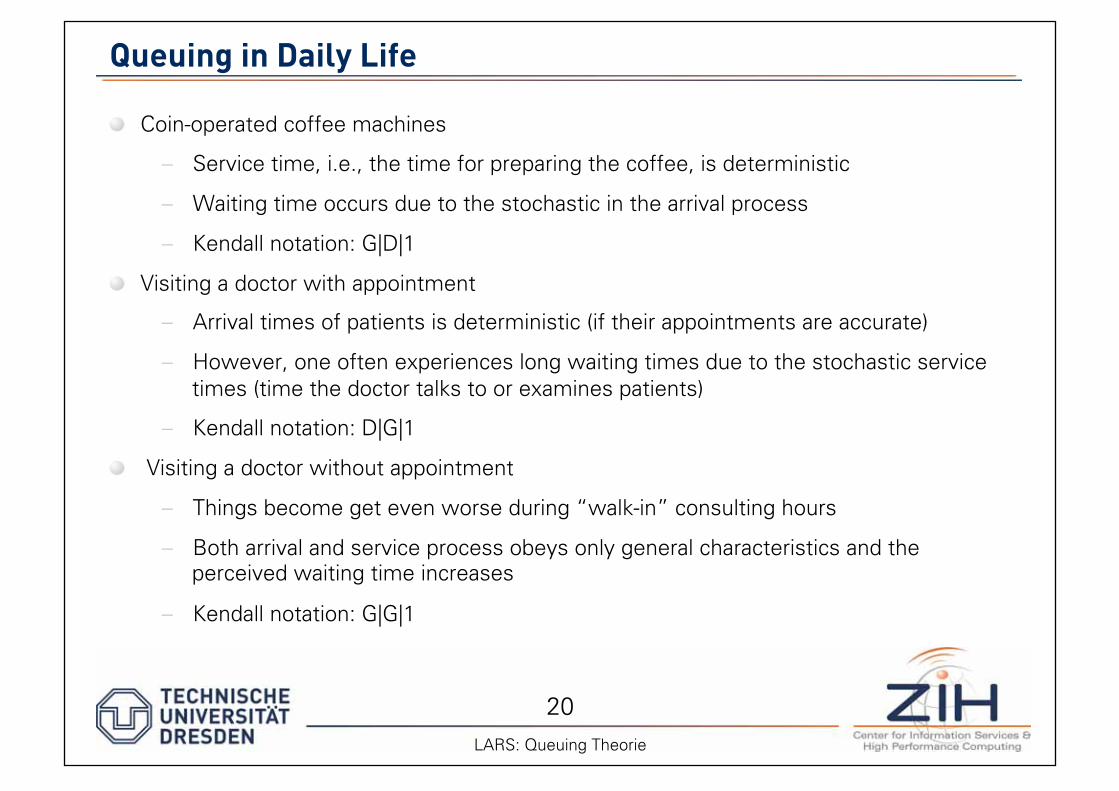
Queuing in Daily Life

Coin-operated coffee machines

– Service time, i.e., the time for preparing the coffee, is deterministic

– Waiting time occurs due to the stochastic in the arrival process

– Kendall notation: G|D|1

Visiting a doctor with appointment

– Arrival times of patients is deterministic (if their appointments are accurate)

– However, one often experiences long waiting times due to the stochastic service times (time the doctor talks to or examines patients)

– Kendall notation: D|G|1

Visiting a doctor without appointment

– Things become get even worse during “walk-in” consulting hours

– Both arrival and service process obeys only general characteristics and the perceived waiting time increases

– Kendall notation: G|G|1


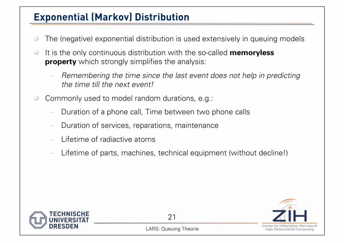
Exponential (Markov) Distribution

The (negative) exponential distribution is used extensively in queuing models

It is the only continuous distribution with the so-called memoryless

property which strongly simplifies the analysis:

– Remembering the time since the last event does not help in predicting the time till the next event!

Commonly used to model random durations, e.g.:

– Duration of a phone call, Time between two phone calls

– Duration of services, reparations, maintenance

– Lifetime of radiactive atoms

– Lifetime of parts, machines, technical equipment (without decline!)


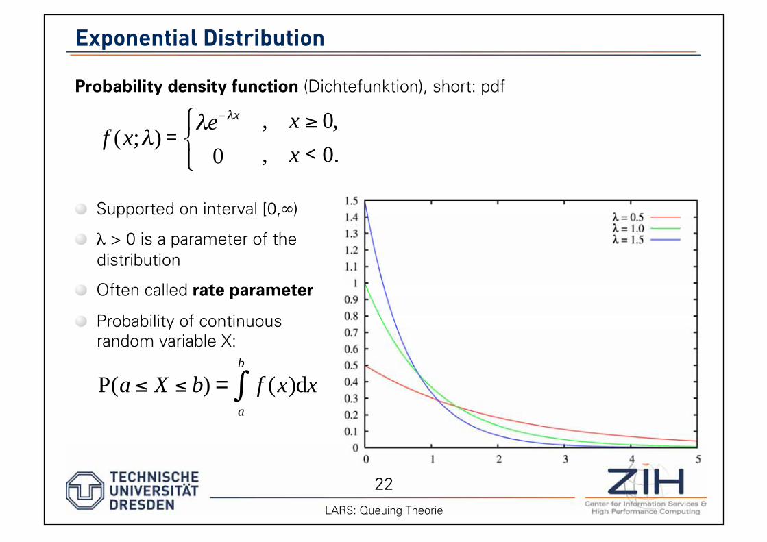
Exponential Distribution

Probability density function (Dichtefunktion), short: pdf

Supported on interval [0, )

> 0 is a parameter of the distribution

Often called rate parameter

Probability of continuous random variable X:

f (x; ) =e x

0

,

,

x 0,

x < 0.

P(a X b) = f (x)dxa

b


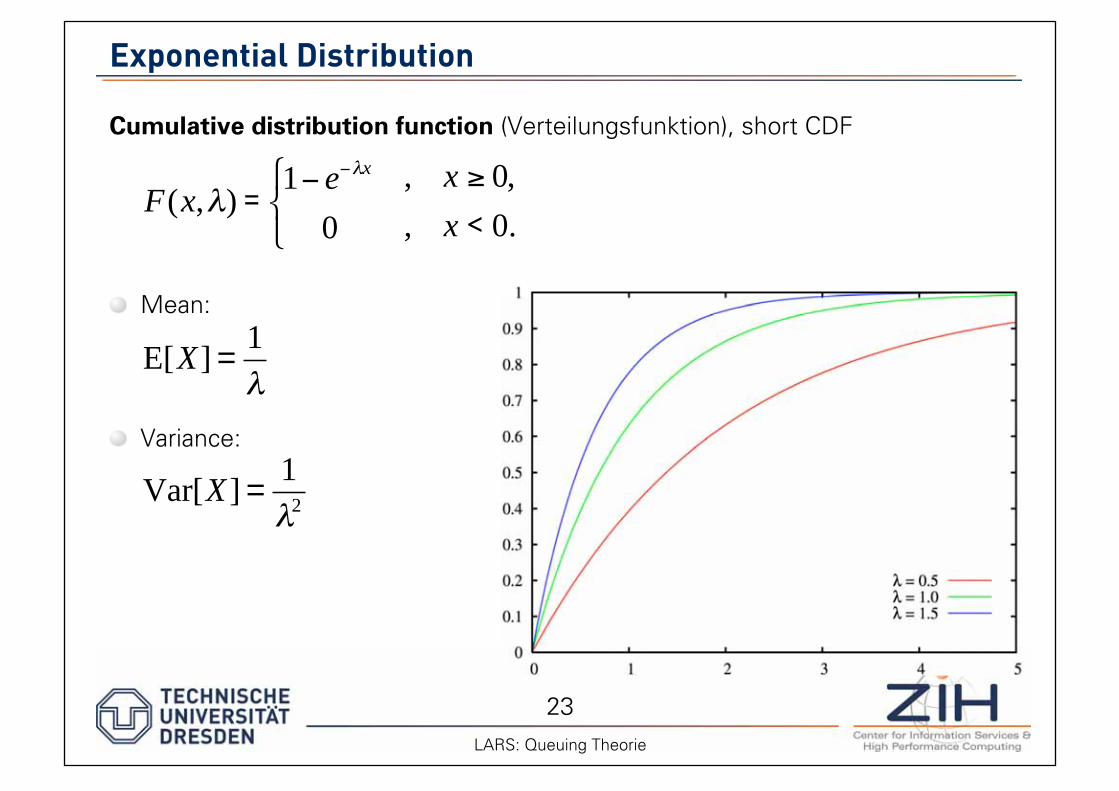
Exponential Distribution

Cumulative distribution function (Verteilungsfunktion), short CDF

Mean:

Variance:

F(x, ) =1 e x

0

,

,

x 0,

x < 0.

E[X] =1

Var[X] =1

2


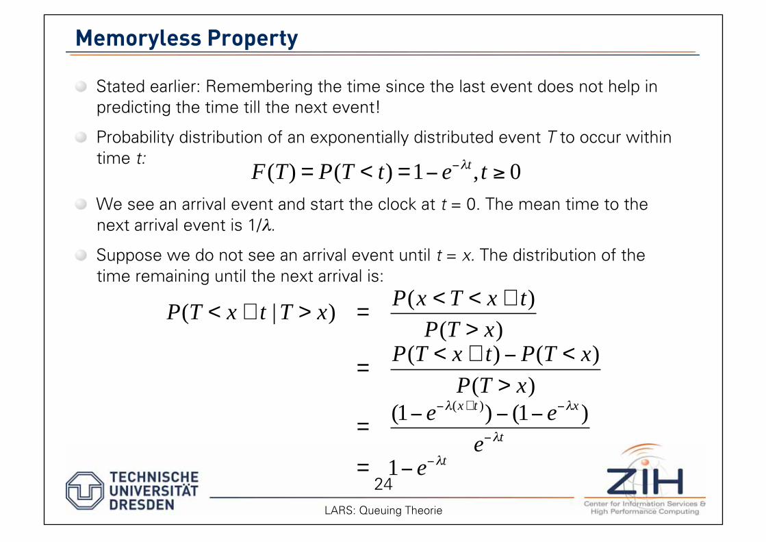
Memoryless Property

Stated earlier: Remembering the time since the last event does not help in predicting the time till the next event!

Probability distribution of an exponentially distributed event T to occur within time t:

We see an arrival event and start the clock at t = 0. The mean time to the next arrival event is 1/ .

Suppose we do not see an arrival event until t = x. The distribution of the time remaining until the next arrival is:

F(T) = P(T < t) =1 e t ,t 0

P(T < x + t |T > x) =P(x < T < x + t)

P(T > x)

=P(T < x + t) P(T < x)

P(T > x)

=(1 e (x+ t )) (1 e x )

e t

= 1 e t


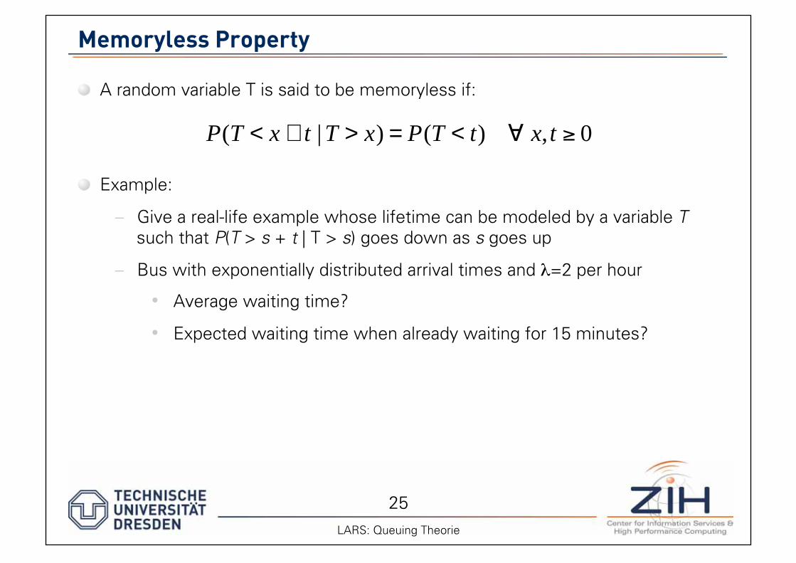
Memoryless Property

A random variable T is said to be memoryless if:

Example:

– Give a real-life example whose lifetime can be modeled by a variable T such that P(T > s + t | T > s) goes down as s goes up

– Bus with exponentially distributed arrival times and =2 per hour

• Average waiting time?

• Expected waiting time when already waiting for 15 minutes?

P(T < x + t |T > x) = P(T < t) x, t 0


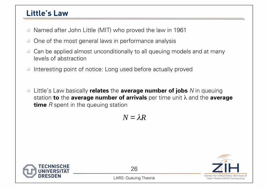
Little’s Law

Named after John Little (MIT) who proved the law in 1961

One of the most general laws in performance analysis

Can be applied almost unconditionally to all queuing models and at many levels of abstraction

Interesting point of notice: Long used before actually proved

Little’s Law basically relates the average number of jobs N in queuing station to the average number of arrivals per time unit and the average

time R spent in the queuing station

N = R


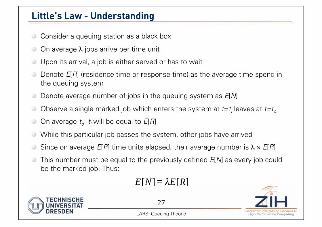
Little’s Law - Understanding

Consider a queuing station as a black box

On average jobs arrive per time unit

Upon its arrival, a job is either served or has to wait

Denote E[R] (residence time or response time) as the average time spend in the queuing system

Denote average number of jobs in the queuing system as E[N]

Observe a single marked job which enters the system at t=ti leaves at t=to.

On average to- ti will be equal to E[R]

While this particular job passes the system, other jobs have arrived

Since on average E[R] time units elapsed, their average number is E[R]

This number must be equal to the previously defined E[N] as every job could be the marked job. Thus:

E[N] = E[R]


Little’s Law - Remarks

We assumed that the queue throughput T equals the arrival rate

Always the case if system is not overloaded and infinite buffers

Otherwise customers will get lost and E[N] = T E[R]

The relationship expressed by Little’s law is valid independently of the form of the involved distributions

This law is valid independently of the scheduling discipline and the number of servers

E[N] is easy to obtain and measures like E[R] can be derived from it

Applies also to networks of queuing stations


Stochastic Processes

Analytical modeling uses several random variables but also stochastic processes which are sequences of random variables

Collection of random variables { X(t) | t T }, indexed by the parameter t (usually time) which can take values of set T

Values that X(t) assumes are called states. All possible states are called state

space I.

The state space and the time parameter can be discrete or continuous

Discrete-state stochastic processes are also called chain, often with I = { 0,1,2,…}

Famous representatives: Markov Process, Birth-Death Process, and Poisson Process (form a hierarchy)


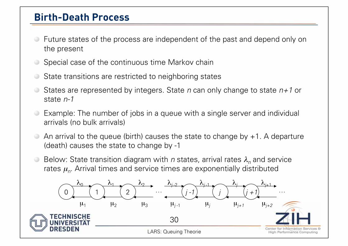
Birth-Death Process

Future states of the process are independent of the past and depend only on the present

Special case of the continuous time Markov chain

State transitions are restricted to neighboring states

States are represented by integers. State n can only change to state n+1 or state n-1

Example: The number of jobs in a queue with a single server and individual arrivals (no bulk arrivals)

An arrival to the queue (birth) causes the state to change by +1. A departure (death) causes the state to change by -1

Below: State transition diagram with n states, arrival rates n and service rates μn. Arrival times and service times are exponentially distributed

0 2 j -1 j j +1 1 0

μ1

1 2

μ2 μ3

j -2 j -1 j j+1 … …

μj -1 μj μj+1 μj+2


Birth-Death Process

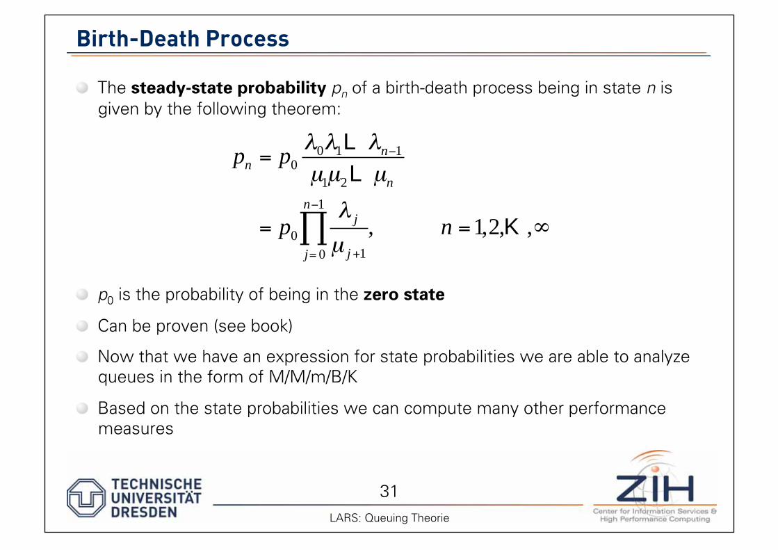
The steady-state probability pn of a birth-death process being in state n is given by the following theorem:

p0 is the probability of being in the zero state

Can be proven (see book)

Now that we have an expression for state probabilities we are able to analyze queues in the form of M/M/m/B/K

Based on the state probabilities we can compute many other performance measures

pn = p00 1L n 1

μ1μ2Lμn

= p0j

μ j+1j= 0

n 1

, n =1,2,K,


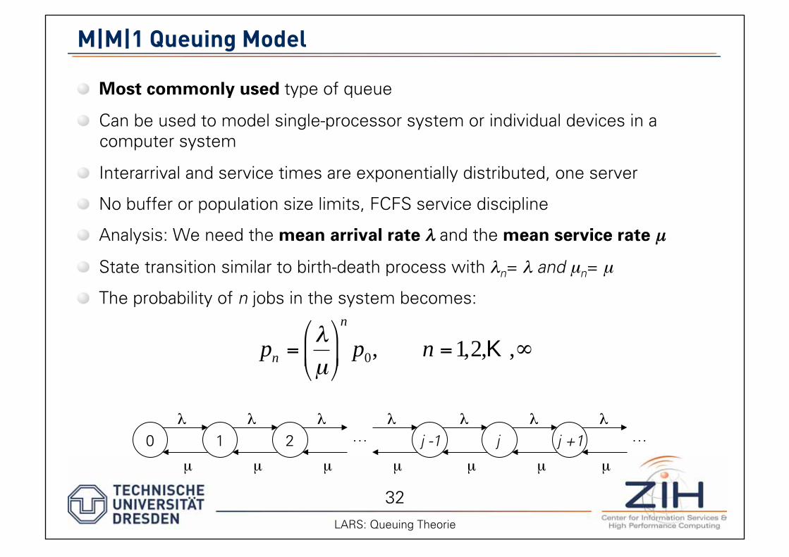
M|M|1 Queuing Model

Most commonly used type of queue

Can be used to model single-processor system or individual devices in a computer system

Interarrival and service times are exponentially distributed, one server

No buffer or population size limits, FCFS service discipline

Analysis: We need the mean arrival rate and the mean service rate μ

State transition similar to birth-death process with n= and μn= μ

The probability of n jobs in the system becomes:

0 2 j -1 j j +1 1

μ

μ μ

… …

μ μ μ μ

pn =μ

n

p0, n =1,2,K,


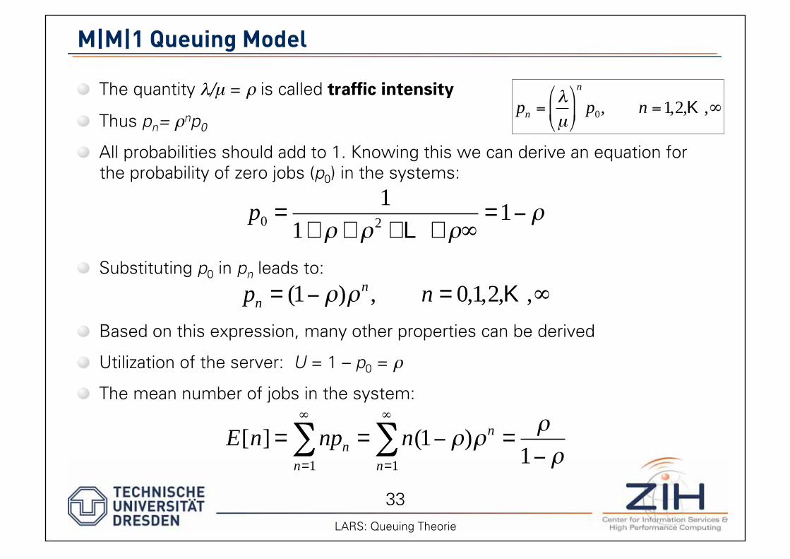
M|M|1 Queuing Model

The quantity /μ = is called traffic intensity

Thus pn= np0

All probabilities should add to 1. Knowing this we can derive an equation for the probability of zero jobs (p0) in the systems:

Substituting p0 in pn leads to:

Based on this expression, many other properties can be derived

Utilization of the server: U = 1 – p0 =

The mean number of jobs in the system:

pn =μ

n

p0, n =1,2,K,

p0 =1

1+ +2+L+

=1

pn = (1 ) n , n = 0,1,2,K,

E[n] = npn = n(1 ) n=

1n=1n=1


M|M|1 Queuing Model

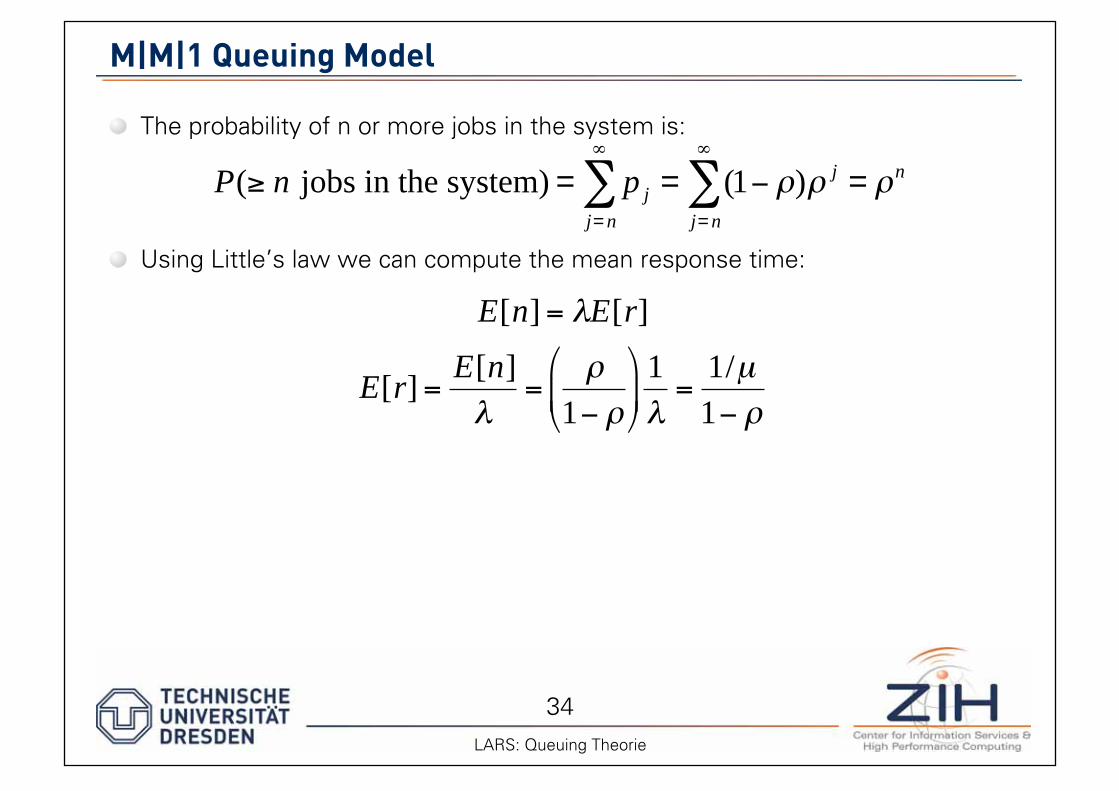
The probability of n or more jobs in the system is:

Using Little’s law we can compute the mean response time:

P( n jobs in the system) = p j = (1 ) j=

n

j= nj= n

E[n] = E[r]

E[r] =E[n]

=1

1

=1/μ

1



Thank You!

Documents

Performance Analysis of Computer Systems - tu-dresden.de fileQueuing/Kendall notation Queuing in daily life Exponential distribution and its memoryless property Little’s law Stochastic