Performance Analysis for Process ImprovementPERFORMANCE ANALYSIS FOR PROCESS IMPROVEMENT ... the process exhibits tool wear and ... sis should assess both the stability of the measurement

PPAslide.pdf

697

PERFORMANCE ANALYSIS FORPROCESS IMPROVEMENT

Michael V. Petrovich

SUMMARY

Process performance analysis, introduced here, uses performance measures such as Pp, Ppk, and Ppm with analy-sis to assess performance, sources of variation, process potential, and improvement opportunity. This analysis maybe conducted where control may not have been achieved and where a large number of process streams exist.

KEY WORDS

performance measures, Ppk, Ppm

INTRODUCTION

The quality goals of an organization include the elimination of nonconformance and the minimization of varia-tion around appropriate targets. The quality practitioner needs to know how well these goals are being realized.Specifically, one must ask, “How well are my processes performing and what must I do to improve?”

For many years process assessment has employed the use of process capability measures. These include Cp, Cpk,and more recently, Cpm. For a review of these see Rodriguez (1992). The use of these measures requires demonstra-tion of statistical control followed by a distribution assessment compared against the targets and specifications.Difficulties arise when statistical control cannot be assumed and also where a large number of process streams maybe present. Here are a few examples.

• A plastic lid manufacturer has 40 molding machines, 54 tools per molder. Tools are replaced every fewweeks, and tool-to-tool differences are found. In addition, slight differences are found as batches of rawmaterials are changed. Other sources of variation include maintenance cycles, startup periods, and anypossible adjustments made by the operating personnel.

• A metal bottlecap company has eight presses, each containing 22 dies. Slight differences exist die-to-dieand press-to-press. In addition, the process exhibits tool wear and slight fluctuations are observed withlot-to-lot changes in steel.

• An aluminum can manufacturer has two lines in one of its plants. Each line contains 16 stations. Station-to-station differences are found. This process also undergoes tool wear and perfect through-time stabil-ity (or control) is not observed in many of the stations.

Traditional capability assessments are inadequate to handle these situations. If control cannot be demonstrated,traditional assessments of process capability cannot be properly made. In addition, the presence of a large number ofprocess streams would yield a combination of distributions that would present a nightmare to mathematically model.

698 ASQ’s 52nd Annual Quality Congress Proceedings

In the meantime, quality practitioners still need a means of assessing their processes and the effectiveness of theirimprovement strategies.

In recent years process performance measures have gained popularity. These measures, introduced by Herman(1989), are analogous to their counterpart capability measures. A “P” representing “performance” replaces the “C”found in “capability” indices. The most popular performance measures are Pp, Ppk, and Ppm. These measures may beused to answer questions concerning how well the process is performing and may be employed before a process isdocumented to be in a state of statistical control.

As introduced here, process performance analysis utilizes performance measures and graphical techniques to dis-play performance, potential performance, and to determine the sources of quality losses. process performance analy-sis provides a means to

• Assess processes before statistical control is achieved• Determine sources of process loss• Make comparisons among characteristics, products, plants, and suppliers• Determine control and improvement priorities• Assess the results of process improvement efforts

SAMPLING

To study processes, samples must be taken and measurements made for critical characteristics. The approachsuggested here is to measure total outgoing variation as sent to the customer. Total outgoing variation results fromvariation inherent to the process as well as variation from lot-to-lot, tool-to-tool, line-to-line, shift-to-shift, setup-to-setup, day-to-day, and throughout maintenance cycles. Sampling will generally be done at end-of-line. To providediagnostic capability, stratified sampling by lines, tools, or other process streams may also be desired.

To assess the performance of a process, and to reflect the total outgoing variation, long periods of data collec-tion with large data sets are preferred. A minimum of one month, and more preferably three months, worth of data isdesired. While the analysis may be done with a few hundred data values, 1000 is a desired minimum; 10,000 or morevalues may be used to provide better analysis. If 100 values were obtained each day, 9000 values would be accumu-lated during a calendar quarter.

Of course, an appropriate measurement system analysis should be conducted prior to data collection. This analy-sis should assess both the stability of the measurement system as well as the variance contributed by measurementerror. The methodology for conducting this type of analysis may be found in numerous texts. See, for example,Chrysler, Ford, and General Motors (1995).

PROCESS PERFORMANCE MEASURES

Process performance measures provide an assessment of processes in which process control may not have beenachieved. These measures take into account all observed variation from both common and special causes, whereastraditional process capability measures consider only the inherent, common cause process variation.

Performance measures assess the historical performance of a process. Any prediction from them would be use-ful only to the extent that the future is expected to resemble the past. To capture total variability in a process, per-formance measures should be assessed from data collected over long periods of time.

When a process is not in a state of control the process distribution is changing through time. Hence, attempts todetermine a specific form of a process distribution would be inappropriate. For this reason, performance measuresshould not consider distributional shape.

Several measures of process performance may be calculated. In this discussion, Ppm, Ppk, and Pp will be shown.Another measure, Pp(process stream), will be used to examine the performance within a process stream. Finally, a poten-tial measure, Cp, will be estimated. Cp may be used to assess the potential of the process. Making comparisons amongthese measures will highlight process losses and improvement opportunities.

Taguchi (1986) defined a loss function which quantifies the losses due to manufacturing variation. As productcharacteristics depart from their design target, this loss function states that the loss will be proportional to the targetdeviation squared. Chan, et al. (1988) created a capability measure, Cpm, which is inversely related to this loss.

The first performance measure discussed here, Ppm, is derived from Cpm and is inversely related to the losses ina manufacturing process. The higher the Ppm value, the better the process performance. When a target, upper, andlower specification are given, Ppm may be calculated by

Ppm 5 5

where

USL is the Upper Specification LimitLSL is the Lower Specification LimitX is the observed valueT is the Targets2 is the sample variance from all combined dataXw is the sample mean from all combined data, andn is the total number of observations

For a single specification and target the following may be used

Ppm 5 5

where SL is the Specification Limit.The use of Ppm assumes valid specifications and targets are given and representative samples are generated dur-

ing the period of interest. When appropriately employed, Ppm may be used as a primary measure to assess the per-formance of a process. Process performance will improve, as measured by increases in Ppm, as the process is broughtinto better control; systematic variation such as differences in tooling, setup, operators, machines, and materials isreduced; and the process is brought on target.

Ppk is recommended when no target is given. Ppk may be calculated as follows.

Ppk 5

Pp is another performance measure which assesses variation but not location. Pp is calculated as follows.

Pp 5 }USL

6

–

s

LSL}

min(USL – Xw, Xw – LSL)}}}

3s

SL – T}}}

3!s2§ 1§ }n§n

–§1}§ (§Xw§ –§ T§)2§

2 SL – T}}}

6!s2§ 1§ }n§n

–§1}§ (§Xw§ –§ T§)2§

USL – LSL}}}

6!s2§ 1§ }n§n

–§1}§ (§Xw§ –§ T§)2§

USL – LSL}}

6!}S§(X§n§–

–§1T§)2

}§

ASQ’s 52nd Annual Quality Congress Proceedings 699

Figure 1. The relationship between Ppm and % Off-Target.

Pp

m


The difference between Ppm and Pp is the term which includes the deviation from target. If the observed processaverage was on target, Ppm and Pp would be identical. Calculation of Pp and making comparisons to Ppm will yieldan understanding of the loss from being off target. An additional diagnostic measure, % Off-Target, may also be cal-culated. This measure represents the percent of the specification range the mean falls from target.

% Off-Target = }U

S

XwL

–

–

T

L

SL

} 3 100%

As the process average departs from target, Ppm is reduced. Figure 1 graphically displays the relationshipbetween Ppm and % Off-Target. The resulting Ppm is shown for four levels of Pp (at infinity, 3, 2, 1.5, 1) as the offsetfrom target varies. The highest line represents a process with a standard deviation of zero (Pp at infinity). If a processis running with a mean 10 percent off target, the largest Ppm that may be achieved is 1.67. At 30 percent off target,the largest Ppm that may be achieved is 0.56.

If the process under study contains multiple lines, tools, or stations (process streams), the losses from differencesbetween these process streams should be understood. Pp(process stream) is a measure of the process performance withinprocess streams. If no process stream differences exist, and the process is on target, Ppm would be equal to Pp(process

stream). Pp(process stream) may be calculated by

Pp (process stream) 5 }6

U

(s

S

wi

L

thi

–

n s

L

tr

S

ea

L

m)}

where swithin stream is the square root of the average of the variances within each process stream calculated by

swithin stream 5!§§§where J is the number of process streams.

A useful diagnostic measure is the percent process stream difference. This measure is simply the range of theprocess stream means divided by the specification range expressed as a percentage.

% Process Stream Difference 5 3 100%

Another important diagnostic assessment concerns the losses which arise from a lack of through-time stabilityor control. The swithin stream includes any sources of through-time variability. The question to answer is, “If perfectthrough-time stability were achieved, how much variation would be observed?” To address this question, the mini-mum potential process variation, spotential, may be estimated. Several approaches may be used for this estimation.Two common approaches are

1) Short-term capability studies2) Estimating variance within process streams using average or median dispersion statistics

Short-term capability studies may be conducted to determine the inherent potential variation of the process. Thismay be done by generating one or more studies of relatively small samples of consecutive items and then estimatingthe potential variability. Preferably, multiple studies should be conducted at different points in time.

Several approaches to estimate the potential variation may be employed when using data sampled over anextended period of time and where control may not be observed. One common approach is to remove individual out-of-control points and to estimate process variation from those points remaining. Unfortunately, this methodology isnot feasible with large data sets.

Another approach to estimate the potential variation is to use averages or medians of dispersion statistics suchas the range, moving range, or standard deviation. These average or median statistics may be used to generate an esti-mated σ by dividing by appropriate constants. [See Wheeler (1995) for tables of constants and methods of calcula-tion.] Median dispersion statistics are more robust to significant shifts in the process than average dispersionstatistics. Although there is more sampling error associated with median dispersion statistics, this is not an issue witha large number of samples.

The potential variation includes measurement error. If desired, measurement error variance may be subtractedfrom this estimate to assess the true product variation (σ2

product = σ2potential – σ2

measurement ). This may be a concern iflarge measurement error variance exists (Herman 1989).

Xwmax stream – Xwmin stream

(n1 – 1) s2stream 1 1 (n2 – 1) s2

stream 2 1 . . . 1 (nJ – 1) s2stream J}}}}}}}

S(nj – 1)


The rate of sampling may influence the estimated potential variation. When using statistics which assess item-to-item variation, shorter time intervals between sampled items would generate lower estimates of potential variance.Sampling consecutive items would result in minimum estimates.

When multiple process streams are present, estimate the potential variation for each process stream. In thesecases, use the average of the estimated standard deviations for estimating process potential, assuming potential vari-ances are equal among process streams. If large differences exist in variation, separate analysis for each processstream may be desired.

Using the estimated potential variation, spotential, a measure of the potential capability of the process, Cp(potential),may be calculated as follows.

Cp (potential) 5 }U6Ss

L

po

–

ten

L

ti

S

al

L}

This potential capability is the potential performance measure (Ppm) that would be obtained if the process werebrought into control, process stream variation was eliminated, and the process was brought on target.

OBSERVED NONCONFORMING RATES

Since distributional analysis is not done with performance measures, and through-time stability may not beachieved, the use of process performance measures should be accompanied with examining the actual observed non-conforming proportion. Using the total number of items examined and the number outside the specification limits thenonconforming proportion may be calculated. Translating the total nonconforming to parts per million (ppm) may beuseful.

Nonconforming Proportion (ppm) 5

PROCESS PERFORMANCE ANALYSIS

The following relationships will hold when generating performance measures.

Ppm ≤ Pp ≤ Pp(process stream) ≤ Cp(potential)

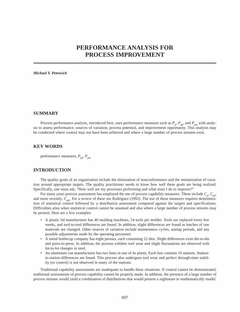
A stacked bar chart may be used to display these relationships. Using the performance measure Ppm as a base,stacked bar charts may be created by using sections which represent the incremental differences between the perfor-mance measures. The height of each section displays the various performance measures. These bar charts show theobserved performance and the improvement potential if the process is brought on target, the process stream variationis removed, and the process is brought into control. An example is shown in Figure 2. These bar charts represent datafrom two plants manufacturing aluminum cans.

1,000,000 × Total Nonconforming}}}}

Total Items

Figure 2. Process performance analysis.

Per

form

ance

The sections of the bars in the chart show the potential performance improvement that would occur in the Ppmvalue when various improvements are made.

• The lowest section of the bars show the observed performance measure, Ppm.• The top of the second section of the bars show the performance had the process average been on target.• The top of the third section of the bars show the performance of the process had the means for each

process stream been on target.• The top of the highest bar sections show the potential of the process if through-time variation is removed

(control achieved) and each process stream mean is on target.

While the areas of the top three bar sections can be thought of as observed losses, these areas cannot be com-pared. The improvement potential seen on the stacked bar chart occurs when the process is brought on target, thenprocess stream differences are removed, and finally through-time stability is achieved. Note that changes in higherbars represent a smaller change in process variation than a change in a lower bar.

The total variance about target, τ2, can be decomposed into the various components that can be compared toassess improvement priority.

τ2 = s2potential + s2

off-target + s2process stream + s2

time

These components may be approximated as follows and displayed in a pie, bar, or Pareto chart.σ2

potential may be estimated as described previously and may also be decomposed into σ2product and σ2

measurement,as described earlier.

σ2off-target may be simply estimated as follows.

s2off-target = (Xw – T)2

The variance from process stream differences may be estimated many ways. If the data have not been stratified,studies may be conducted to determine the variance contribution from process stream differences. These studies mayinclude all streams of interest or a random selection of streams. Methods such as analysis of variance (ANOVA) maybe used to estimate this component. Remember though, that the process is not assumed to be stable and these assess-ments should be considered approximate. If the data have been stratified by all process streams of interest, the processstream variance may be simply estimated as follows.

s2process stream = s2 – s2

within stream

where, again, s2 is the sample variance from all combined data.The variance from through-time process changes, σ2

time, may be estimated as follows.

s 2time 5 s 2

within stream – s2potential


Figure 3. A histogram of the data.

Freq

uenc

y


Figure 5. Process performance analysis stacked bar chart.

Figure 6. An extension of the stacked bar chart.

Figure 4. Box & whisker plots.

Per

form

ance

Per

form

ance


Figure 7. Pie chart of the variance components.

Figure 8. Combined data through time.

Figure 9. Control chart of data, part 1.

Indi

vidu

al V

alue

sS

igm

aIn

divi

dual

Val

ues

Mov

ing

Ran

ge


EXAMPLE

Aluminum lids are produced on a machine with 22 stations. Each day, lids from each station are sampled andthe lid height is measured. Data are collected over a three-month period. The specifications for this characteristic are98 ± 5. Table 1 provides an analysis of these data.

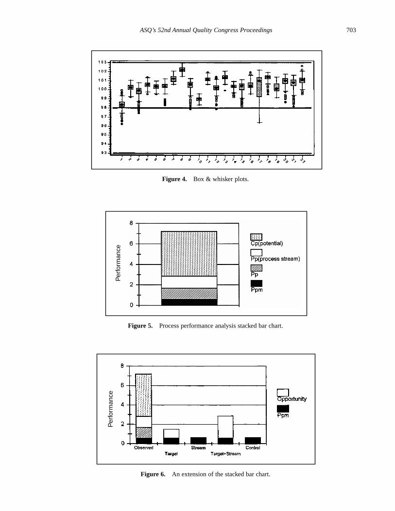
Figure 10. Control chart of data, part 2.

Figure 11. Run chart of data, part 1.

Figure 12. Run chart of data, part 2.

Indi

vidu

al V

alue

sM

ovin

g R

ange

Val

ues

Val

ues

Table 1 displays the descriptive measures, the variance components, and the performance calculations. Figure 3displays a histogram of all the data. Figure 4 displays box and whisker plots for each of the 22 stations with the tar-get and specifications. Figure 5 displays a process performance analysis stacked bar chart. Figure 6 shows an exten-sion of the stacked bar chart. Figure 6 shows the original stacked bar chart plus the effects on performance for variousimprovements. The second bar height shows the performance if brought on target, the third shows the performanceif the process stream differences were removed, the fourth shows both the target and stream effects removed, and thefifth shows the effect if the through-time instability was removed.

Figure 7 displays a pie chart of the variance components. Figure 8 shows the combined data through time.Figures 9 and 10 show control charts for two stations. The same data from these stations are displayed in Figures 11and 12 on a run chart with the specifications drawn.

From these charts, it can be seen that the biggest opportunity comes from getting the individual stations on tar-get. While improvement in control will minimize variation, the through-time sources of variability do not representthe largest opportunity. Measurement error analysis is not shown, but from the process potential assessment, mea-surement error may be considered negligible.

These results are typical of many observed processes. Improvements in targeting and reduction of stream-to-stream differences often represent an important opportunity. While improvement in through-time stability or controldoes not represent a large improvement opportunity in this case, it may be critical in others.


Table 1. Performance analysis—height.

Descriptives:

SQRT (MSW) = 0.5823 (Within Stream Std Dev)AVG Std (Median MR) = 0.2311 (Potential within Stream Std Dev)

n = 2948Mean = 100.4816

Std Dev = 0.9788Low = 96.2600

Q1 = 100.0650Median = 100.5900

Q3 = 101.1400High = 102.9400

Skewness = -0.7319Kurtosis = 0.7588

Variance Components:

Potential = 0.0534 (0.75%)Target Loss = 6.1583 (86.54%)

Time (control) = 0.2857 (4.01%)Stream-Stream = 0.6190 (8.7%)

Performance:

% Off Target = 24.82% Max Stream Mean = 102.2103 % Stream Loss = 38.42% Min Stream Mean = 98.3680

Ppk = 0.858 Above USL = 0Ppm = 0.625 Below LSL = 0

Pp = 1.703 Total Out = 0 (0 ppm)Pp (Stream) = 2.862 n = 2948

Cp (pot) = 7.212

CONCLUSION

The use of process performance measures generated with data collected over extended periods, combined withperformance analysis which decomposes sources of variation, provides quality practitioners the ability to answerquestions about how their processes are performing and what opportunities exist for improvement. The graphical dis-play of these measures allows one to view the improvement potential. This display may be used to compare multipleprocesses and characteristics and assist in improvement prioritization. Performance measures such as the Ppm may beused to validate improvement efforts. If through-time stability is improved, tooling or station differences are mini-mized, and the process is brought on target, Ppm will display an improvement.

REFERENCES

Chrysler Corporation, Ford Motor Company, General Motors Corporation. 1995. Measurement Systems Analysis.Southfield, MI: Automotive Industry Action Group (AIAG).

Herman, John T. 1989. Capability Index—Enough for Process Industries? 1989—ASQC Quality CongressTransactions. 92–104.

Rodriguez, Robert N. 1992. Recent Developments in Process Capability Analysis. Journal of Quality Technology,Vol. 24, No. 4, 176–187.

Chan, Lai K., Cheng, Smiley W., and Spiring, Frederick A. 1988. A New Measures of Process Capability: Cpm,Journal of Quality Technology, Vol.20, No. 3, 162–175.

Taguchi, G. 1986. Introduction to Quality Engineering. Tokyo, Japan: Asian Productivity Organization.Wheeler, Donald J. 1995. Advanced Topics in Statistical Process Control. Knoxville, TN: SPC Press.


Documents

Performance Analysis for Process ImprovementPERFORMANCE ANALYSIS FOR PROCESS IMPROVEMENT ... the process exhibits tool wear and ... sis should assess both the stability of the measurement