Perception-Driven Semi-Structured Boundary Vectorization

SHAYAN HOSHYARI, University of British ColumbiaEDOARDO ALBERTO DOMINICI, University of British ColumbiaALLA SHEFFER, University of British ColumbiaNATHAN CARR, AdobeZHAOWEN WANG, AdobeDUYGU CEYLAN, AdobeI-CHAO SHEN, National Taiwan University

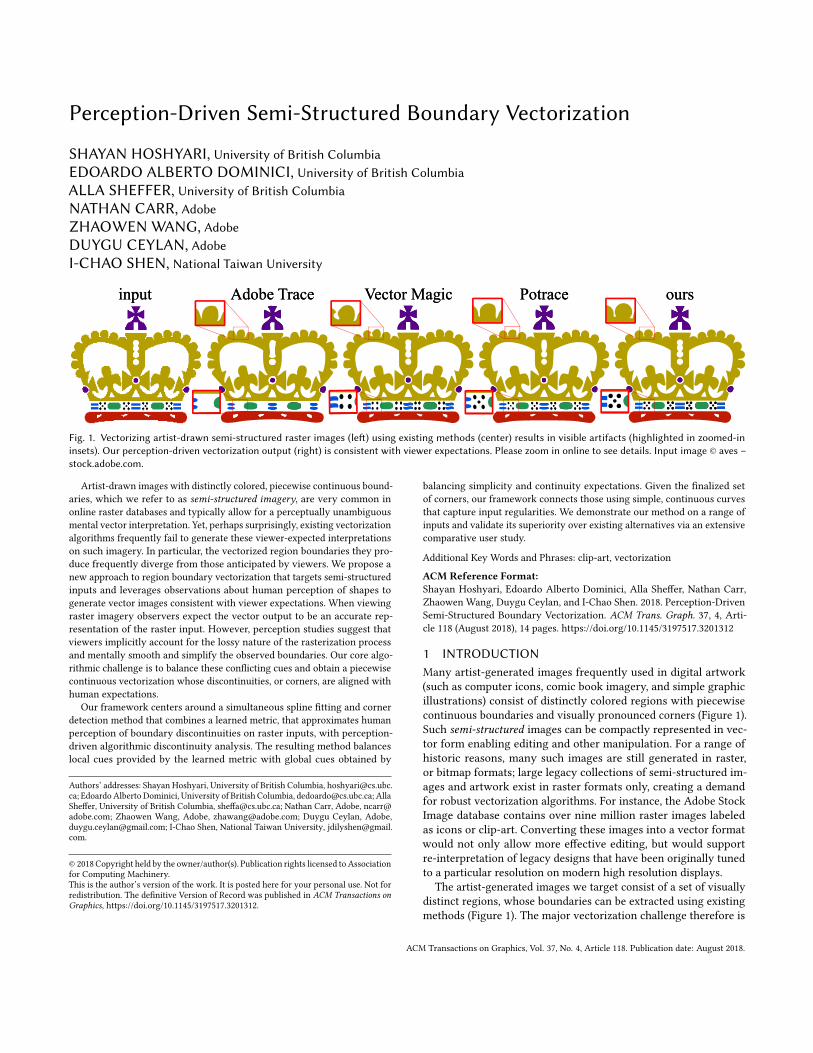
input Adobe Trace Vector Magic Potraceinput Adobe Trace Vector Magic Potrace oursours

Fig. 1. Vectorizing artist-drawn semi-structured raster images (left) using existing methods (center) results in visible artifacts (highlighted in zoomed-ininsets). Our perception-driven vectorization output (right) is consistent with viewer expectations. Please zoom in online to see details. Input image © aves –stock.adobe.com.

Artist-drawn images with distinctly colored, piecewise continuous bound-

aries, which we refer to as semi-structured imagery, are very common in

online raster databases and typically allow for a perceptually unambiguous

mental vector interpretation. Yet, perhaps surprisingly, existing vectorization

algorithms frequently fail to generate these viewer-expected interpretations

on such imagery. In particular, the vectorized region boundaries they pro-

duce frequently diverge from those anticipated by viewers. We propose a

new approach to region boundary vectorization that targets semi-structured

inputs and leverages observations about human perception of shapes to

generate vector images consistent with viewer expectations. When viewing

raster imagery observers expect the vector output to be an accurate rep-

resentation of the raster input. However, perception studies suggest that

viewers implicitly account for the lossy nature of the rasterization process

and mentally smooth and simplify the observed boundaries. Our core algo-

rithmic challenge is to balance these conflicting cues and obtain a piecewise

continuous vectorization whose discontinuities, or corners, are aligned with

human expectations.

Our framework centers around a simultaneous spline fitting and corner

detection method that combines a learned metric, that approximates human

perception of boundary discontinuities on raster inputs, with perception-

driven algorithmic discontinuity analysis. The resulting method balances

local cues provided by the learned metric with global cues obtained by

Authors’ addresses: Shayan Hoshyari, University of British Columbia, hoshyari@cs.ubc.

ca; Edoardo Alberto Dominici, University of British Columbia, dedoardo@cs.ubc.ca; Alla

Sheffer, University of British Columbia, sheffa@cs.ubc.ca; Nathan Carr, Adobe, ncarr@

adobe.com; Zhaowen Wang, Adobe, zhawang@adobe.com; Duygu Ceylan, Adobe,

duygu.ceylan@gmail.com; I-Chao Shen, National Taiwan University, jdilyshen@gmail.

com.

© 2018 Copyright held by the owner/author(s). Publication rights licensed to Association

for Computing Machinery.

This is the author’s version of the work. It is posted here for your personal use. Not for

redistribution. The definitive Version of Record was published in ACM Transactions onGraphics, https://doi.org/10.1145/3197517.3201312.

balancing simplicity and continuity expectations. Given the finalized set

of corners, our framework connects those using simple, continuous curves

that capture input regularities. We demonstrate our method on a range of

inputs and validate its superiority over existing alternatives via an extensive

comparative user study.

Additional Key Words and Phrases: clip-art, vectorization

ACM Reference Format:Shayan Hoshyari, Edoardo Alberto Dominici, Alla Sheffer, Nathan Carr,

Zhaowen Wang, Duygu Ceylan, and I-Chao Shen. 2018. Perception-Driven

Semi-Structured Boundary Vectorization. ACM Trans. Graph. 37, 4, Arti-cle 118 (August 2018), 14 pages. https://doi.org/10.1145/3197517.3201312

1 INTRODUCTIONMany artist-generated images frequently used in digital artwork

(such as computer icons, comic book imagery, and simple graphic

illustrations) consist of distinctly colored regions with piecewise

continuous boundaries and visually pronounced corners (Figure 1).

Such semi-structured images can be compactly represented in vec-

tor form enabling editing and other manipulation. For a range of

historic reasons, many such images are still generated in raster,

or bitmap formats; large legacy collections of semi-structured im-

ages and artwork exist in raster formats only, creating a demand

for robust vectorization algorithms. For instance, the Adobe Stock

Image database contains over nine million raster images labeled

as icons or clip-art. Converting these images into a vector format

would not only allow more effective editing, but would support

re-interpretation of legacy designs that have been originally tuned

to a particular resolution on modern high resolution displays.

The artist-generated images we target consist of a set of visually

distinct regions, whose boundaries can be extracted using existing

methods (Figure 1). The major vectorization challenge therefore is

ACM Transactions on Graphics, Vol. 37, No. 4, Article 118. Publication date: August 2018.

118:2 • Shayan Hoshyari, Edoardo Alberto Dominici, Alla Sheffer, Nathan Carr, Zhaowen Wang, Duygu Ceylan, and I-Chao Shen

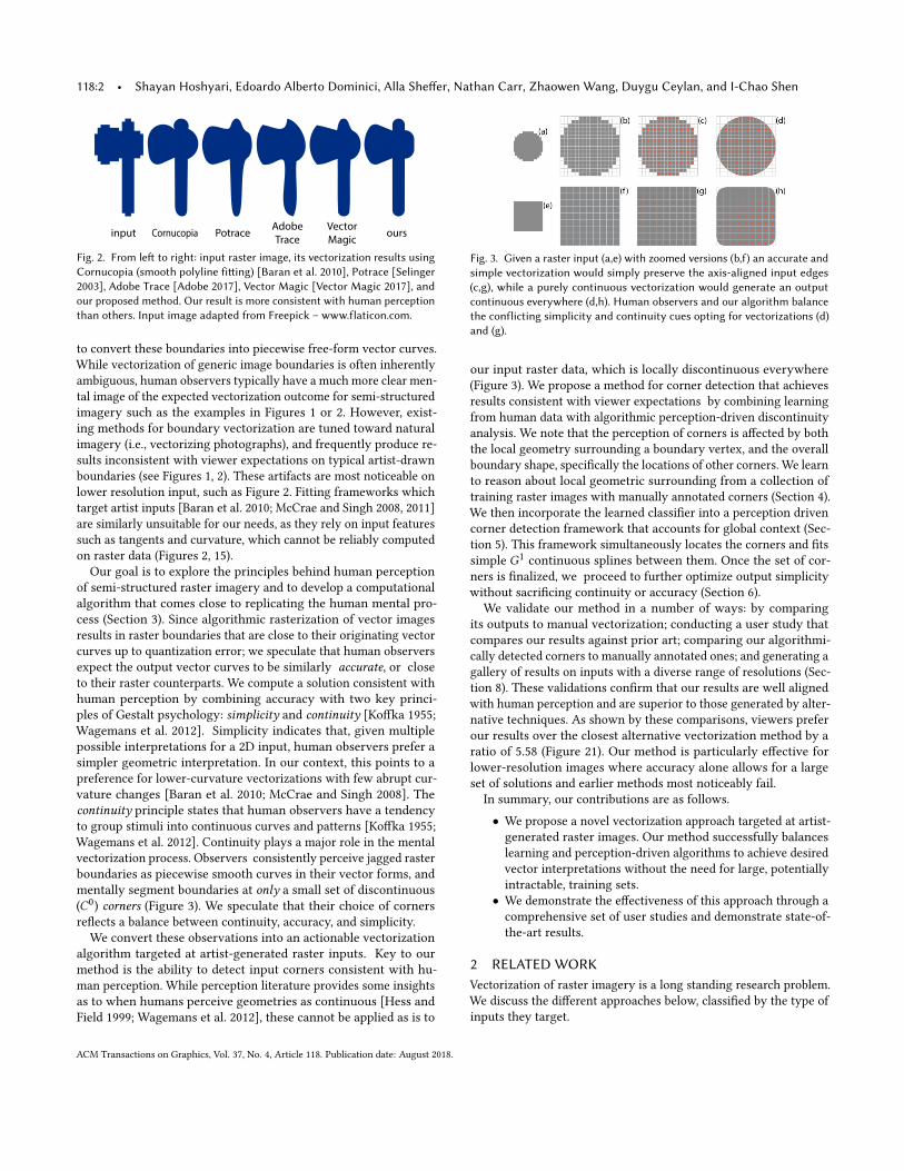
input Cornucopia Potrace AdobeTrace

VectorMagic ours

Fig. 2. From left to right: input raster image, its vectorization results usingCornucopia (smooth polyline fitting) [Baran et al. 2010], Potrace [Selinger2003], Adobe Trace [Adobe 2017], Vector Magic [Vector Magic 2017], andour proposed method. Our result is more consistent with human perceptionthan others. Input image adapted from Freepick – www.flaticon.com.

to convert these boundaries into piecewise free-form vector curves.

While vectorization of generic image boundaries is often inherently

ambiguous, human observers typically have a much more clear men-

tal image of the expected vectorization outcome for semi-structured

imagery such as the examples in Figures 1 or 2. However, exist-

ing methods for boundary vectorization are tuned toward natural

imagery (i.e., vectorizing photographs), and frequently produce re-

sults inconsistent with viewer expectations on typical artist-drawn

boundaries (see Figures 1, 2). These artifacts are most noticeable on

lower resolution input, such as Figure 2. Fitting frameworks which

target artist inputs [Baran et al. 2010; McCrae and Singh 2008, 2011]

are similarly unsuitable for our needs, as they rely on input features

such as tangents and curvature, which cannot be reliably computed

on raster data (Figures 2, 15).

Our goal is to explore the principles behind human perception

of semi-structured raster imagery and to develop a computational

algorithm that comes close to replicating the human mental pro-

cess (Section 3). Since algorithmic rasterization of vector images

results in raster boundaries that are close to their originating vector

curves up to quantization error; we speculate that human observers

expect the output vector curves to be similarly accurate, or close

to their raster counterparts. We compute a solution consistent with

human perception by combining accuracy with two key princi-

ples of Gestalt psychology: simplicity and continuity [Koffka 1955;

Wagemans et al. 2012]. Simplicity indicates that, given multiple

possible interpretations for a 2D input, human observers prefer a

simpler geometric interpretation. In our context, this points to a

preference for lower-curvature vectorizations with few abrupt cur-

vature changes [Baran et al. 2010; McCrae and Singh 2008]. The

continuity principle states that human observers have a tendency

to group stimuli into continuous curves and patterns [Koffka 1955;

Wagemans et al. 2012]. Continuity plays a major role in the mental

vectorization process. Observers consistently perceive jagged raster

boundaries as piecewise smooth curves in their vector forms, and

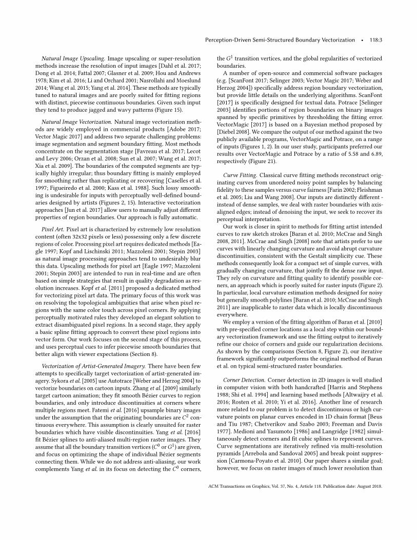
mentally segment boundaries at only a small set of discontinuous

(C0) corners (Figure 3). We speculate that their choice of corners

reflects a balance between continuity, accuracy, and simplicity.

We convert these observations into an actionable vectorization

algorithm targeted at artist-generated raster inputs. Key to our

method is the ability to detect input corners consistent with hu-

man perception. While perception literature provides some insights

as to when humans perceive geometries as continuous [Hess and

Field 1999; Wagemans et al. 2012], these cannot be applied as is to

Fig. 3. Given a raster input (a,e) with zoomed versions (b,f) an accurate andsimple vectorization would simply preserve the axis-aligned input edges(c,g), while a purely continuous vectorization would generate an outputcontinuous everywhere (d,h). Human observers and our algorithm balancethe conflicting simplicity and continuity cues opting for vectorizations (d)and (g).

our input raster data, which is locally discontinuous everywhere

(Figure 3). We propose a method for corner detection that achieves

results consistent with viewer expectations by combining learning

from human data with algorithmic perception-driven discontinuity

analysis. We note that the perception of corners is affected by both

the local geometry surrounding a boundary vertex, and the overall

boundary shape, specifically the locations of other corners. We learn

to reason about local geometric surrounding from a collection of

training raster images with manually annotated corners (Section 4).

We then incorporate the learned classifier into a perception driven

corner detection framework that accounts for global context (Sec-

tion 5). This framework simultaneously locates the corners and fits

simple G1continuous splines between them. Once the set of cor-

ners is finalized, we proceed to further optimize output simplicity

without sacrificing continuity or accuracy (Section 6).

We validate our method in a number of ways: by comparing

its outputs to manual vectorization; conducting a user study that

compares our results against prior art; comparing our algorithmi-

cally detected corners to manually annotated ones; and generating a

gallery of results on inputs with a diverse range of resolutions (Sec-

tion 8). These validations confirm that our results are well aligned

with human perception and are superior to those generated by alter-

native techniques. As shown by these comparisons, viewers prefer

our results over the closest alternative vectorization method by a

ratio of 5.58 (Figure 21). Our method is particularly effective for

lower-resolution images where accuracy alone allows for a large

set of solutions and earlier methods most noticeably fail.

In summary, our contributions are as follows.

• We propose a novel vectorization approach targeted at artist-

generated raster images. Our method successfully balances

learning and perception-driven algorithms to achieve desired

vector interpretations without the need for large, potentially

intractable, training sets.

• We demonstrate the effectiveness of this approach through a

comprehensive set of user studies and demonstrate state-of-

the-art results.

2 RELATED WORKVectorization of raster imagery is a long standing research problem.

We discuss the different approaches below, classified by the type of

inputs they target.

ACM Transactions on Graphics, Vol. 37, No. 4, Article 118. Publication date: August 2018.

Perception-Driven Semi-Structured Boundary Vectorization • 118:3

Natural Image Upscaling. Image upscaling or super-resolution

methods increase the resolution of input images [Dahl et al. 2017;

Dong et al. 2014; Fattal 2007; Glasner et al. 2009; Hou and Andrews

1978; Kim et al. 2016; Li and Orchard 2001; Nasrollahi and Moeslund

2014; Wang et al. 2015; Yang et al. 2014]. These methods are typically

tuned to natural images and are poorly suited for fitting regions

with distinct, piecewise continuous boundaries. Given such input

they tend to produce jagged and wavy patterns (Figure 15).

Natural Image Vectorization. Natural image vectorization meth-

ods are widely employed in commercial products [Adobe 2017;

Vector Magic 2017] and address two separate challenging problems:

image segmentation and segment boundary fitting. Most methods

concentrate on the segmentation stage [Favreau et al. 2017; Lecot

and Levy 2006; Orzan et al. 2008; Sun et al. 2007; Wang et al. 2017;

Xia et al. 2009]. The boundaries of the computed segments are typ-

ically highly irregular; thus boundary fitting is mainly employed

for smoothing rather than replicating or recovering [Caselles et al.

1997; Figueiredo et al. 2000; Kass et al. 1988]. Such lossy smooth-

ing is undesirable for inputs with perceptually well-defined bound-

aries designed by artists (Figures 2, 15). Interactive vectorization

approaches [Jun et al. 2017] allow users to manually adjust different

properties of region boundaries. Our approach is fully automatic.

Pixel Art. Pixel art is characterized by extremely low resolution

content (often 32x32 pixels or less) possessing only a few discrete

regions of color. Processing pixel art requires dedicated methods [Ea-

gle 1997; Kopf and Lischinski 2011; Mazzoleni 2001; Stepin 2003]

as natural image processing approaches tend to undesirably blur

this data. Upscaling methods for pixel art [Eagle 1997; Mazzoleni

2001; Stepin 2003] are intended to run in real-time and are often

based on simple strategies that result in quality degradation as res-

olution increases. Kopf et al. [2011] proposed a dedicated method

for vectorizing pixel art data. The primary focus of this work was

on resolving the topological ambiguities that arise when pixel re-

gions with the same color touch across pixel corners. By applying

perceptually motivated rules they developed an elegant solution to

extract disambiguated pixel regions. In a second stage, they apply

a basic spline fitting approach to convert these pixel regions into

vector form. Our work focuses on the second stage of this process,

and uses perceptual cues to infer piecewise smooth boundaries that

better align with viewer expectations (Section 8).

Vectorization of Artist-Generated Imagery. There have been few

attempts to specifically target vectorization of artist-generated im-

agery. Sykora et al. [2005] use Autotrace [Weber and Herzog 2004] to

vectorize boundaries on cartoon inputs. Zhang et al. [2009] similarly

target cartoon animation; they fit smooth Bézier curves to region

boundaries, and only introduce discontinuities at corners where

multiple regions meet. Fatemi et al. [2016] upsample binary images

under the assumption that the originating boundaries are C2con-

tinuous everywhere. This assumption is clearly unsuited for raster

boundaries which have visible discontinuities. Yang et al. [2016]fit Bézier splines to anti-aliased multi-region raster images. They

assume that all the boundary transition vertices (C0orG1

) are given,

and focus on optimizing the shape of individual Bézier segments

connecting them. While we do not address anti-aliasing, our work

complements Yang et al. in its focus on detecting the C0corners,

the G1transition vertices, and the global regularities of vectorized

boundaries.

A number of open-source and commercial software packages

(e.g. [ScanFont 2017; Selinger 2003; Vector Magic 2017; Weber and

Herzog 2004]) specifically address region boundary vectorization,

but provide little details on the underlying algorithms. ScanFont

[2017] is specifically designed for textual data. Potrace [Selinger

2003] identifies portions of region boundaries on binary images

spanned by specific primitives by thresholding the fitting error.

VectorMagic [2017] is based on a Bayesian method proposed by

[Diebel 2008]. We compare the output of our method against the two

publicly available programs, VectorMagic and Potrace, on a range

of inputs (Figures 1, 2). In our user study, participants preferred our

results over VectorMagic and Potrace by a ratio of 5.58 and 6.89,

respectively (Figure 21).

Curve Fitting. Classical curve fitting methods reconstruct orig-

inating curves from unordered noisy point samples by balancing

fidelity to these samples versus curve fairness [Farin 2002; Fleishman

et al. 2005; Liu and Wang 2008]. Our inputs are distinctly different -

instead of dense samples, we deal with raster boundaries with axis-

aligned edges; instead of denoising the input, we seek to recover its

perceptual interpretation.

Our work is closer in spirit to methods for fitting artist intended

curves to raw sketch strokes [Baran et al. 2010; McCrae and Singh

2008, 2011]. McCrae and Singh [2008] note that artists prefer to use

curves with linearly changing curvature and avoid abrupt curvature

discontinuities, consistent with the Gestalt simplicity cue. These

methods consequently look for a compact set of simple curves, with

gradually changing curvature, that jointly fit the dense raw input.

They rely on curvature and fitting quality to identify possible cor-

ners, an approach which is poorly suited for raster inputs (Figure 2).

In particular, local curvature estimation methods designed for noisy

but generally smooth polylines [Baran et al. 2010; McCrae and Singh

2011] are inapplicable to raster data which is locally discontinuous

everywhere.

We employ a version of the fitting algorithm of Baran et al. [2010]

with pre-specified corner locations as a local step within our bound-

ary vectorization framework and use the fitting output to iteratively

refine our choice of corners and guide our regularization decisions.

As shown by the comparisons (Section 8, Figure 2), our iterative

framework significantly outperforms the original method of Baran

et al. on typical semi-structured raster boundaries.

Corner Detection. Corner detection in 2D images is well studied

in computer vision with both handcrafted [Harris and Stephens

1988; Shi et al. 1994] and learning based methods [Altwaijry et al.

2016; Rosten et al. 2010; Yi et al. 2016]. Another line of research

more related to our problem is to detect discontinuous or high cur-

vature points on planar curves encoded in 1D chain format [Beus

and Tiu 1987; Chetverikov and Szabo 2003; Freeman and Davis

1977]. Medioni and Yasumoto [1986] and Langridge [1982] simul-

taneously detect corners and fit cubic splines to represent curves.

Curve segmentations are iteratively refined via multi-resolution

pyramids [Arrebola and Sandoval 2005] and break point suppres-

sion [Carmona-Poyato et al. 2010]. Our paper shares a similar goal;

however, we focus on raster images of much lower resolution than

ACM Transactions on Graphics, Vol. 37, No. 4, Article 118. Publication date: August 2018.

118:4 • Shayan Hoshyari, Edoardo Alberto Dominici, Alla Sheffer, Nathan Carr, Zhaowen Wang, Duygu Ceylan, and I-Chao Shen

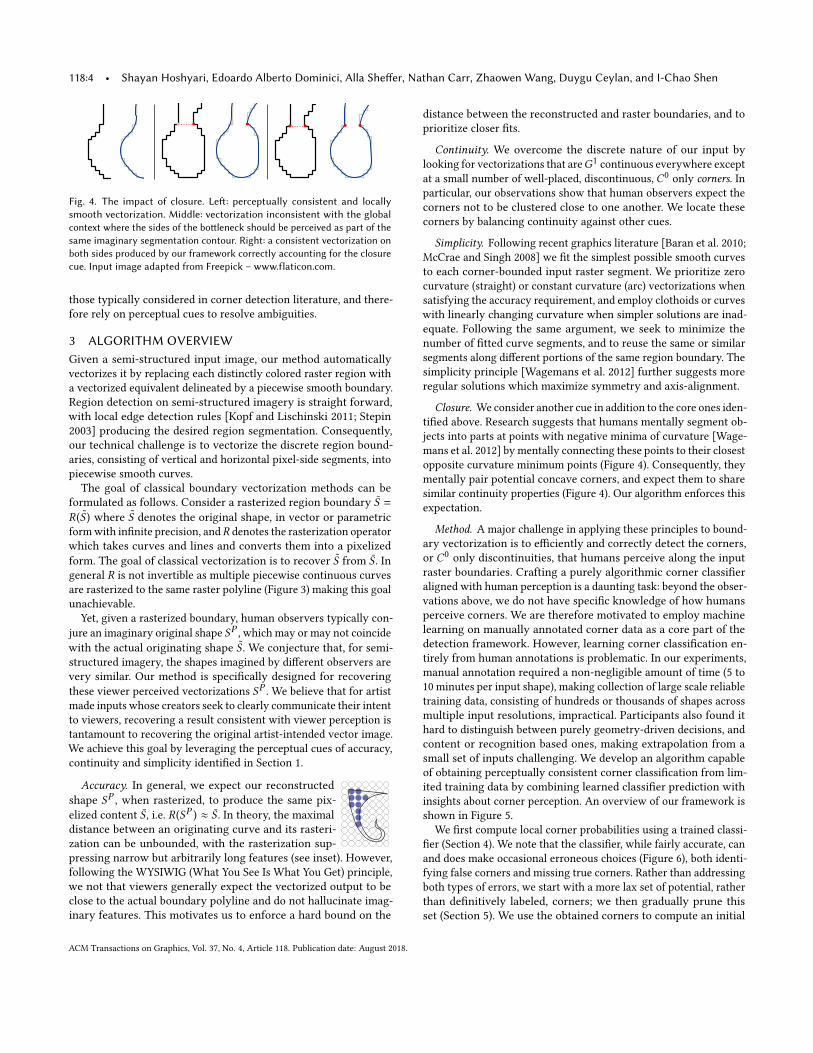
Fig. 4. The impact of closure. Left: perceptually consistent and locallysmooth vectorization. Middle: vectorization inconsistent with the globalcontext where the sides of the bottleneck should be perceived as part of thesame imaginary segmentation contour. Right: a consistent vectorization onboth sides produced by our framework correctly accounting for the closurecue. Input image adapted from Freepick – www.flaticon.com.

those typically considered in corner detection literature, and there-

fore rely on perceptual cues to resolve ambiguities.

3 ALGORITHM OVERVIEWGiven a semi-structured input image, our method automatically

vectorizes it by replacing each distinctly colored raster region with

a vectorized equivalent delineated by a piecewise smooth boundary.

Region detection on semi-structured imagery is straight forward,

with local edge detection rules [Kopf and Lischinski 2011; Stepin

2003] producing the desired region segmentation. Consequently,

our technical challenge is to vectorize the discrete region bound-

aries, consisting of vertical and horizontal pixel-side segments, into

piecewise smooth curves.

The goal of classical boundary vectorization methods can be

formulated as follows. Consider a rasterized region boundary S =R (S ) where S denotes the original shape, in vector or parametric

formwith infinite precision, andR denotes the rasterization operator

which takes curves and lines and converts them into a pixelized

form. The goal of classical vectorization is to recover S from S . Ingeneral R is not invertible as multiple piecewise continuous curves

are rasterized to the same raster polyline (Figure 3) making this goal

unachievable.

Yet, given a rasterized boundary, human observers typically con-

jure an imaginary original shape SP , which may or may not coincide

with the actual originating shape S . We conjecture that, for semi-

structured imagery, the shapes imagined by different observers are

very similar. Our method is specifically designed for recovering

these viewer perceived vectorizations SP . We believe that for artist

made inputs whose creators seek to clearly communicate their intent

to viewers, recovering a result consistent with viewer perception is

tantamount to recovering the original artist-intended vector image.

We achieve this goal by leveraging the perceptual cues of accuracy,

continuity and simplicity identified in Section 1.

Accuracy. In general, we expect our reconstructed

shape SP , when rasterized, to produce the same pix-

elized content S , i.e. R (SP ) ≈ S . In theory, the maximal

distance between an originating curve and its rasteri-

zation can be unbounded, with the rasterization sup-

pressing narrow but arbitrarily long features (see inset). However,

following the WYSIWIG (What You See Is What You Get) principle,

we not that viewers generally expect the vectorized output to be

close to the actual boundary polyline and do not hallucinate imag-

inary features. This motivates us to enforce a hard bound on the

distance between the reconstructed and raster boundaries, and to

prioritize closer fits.

Continuity. We overcome the discrete nature of our input by

looking for vectorizations that areG1continuous everywhere except

at a small number of well-placed, discontinuous, C0only corners. In

particular, our observations show that human observers expect the

corners not to be clustered close to one another. We locate these

corners by balancing continuity against other cues.

Simplicity. Following recent graphics literature [Baran et al. 2010;

McCrae and Singh 2008] we fit the simplest possible smooth curves

to each corner-bounded input raster segment. We prioritize zero

curvature (straight) or constant curvature (arc) vectorizations when

satisfying the accuracy requirement, and employ clothoids or curves

with linearly changing curvature when simpler solutions are inad-

equate. Following the same argument, we seek to minimize the

number of fitted curve segments, and to reuse the same or similar

segments along different portions of the same region boundary. The

simplicity principle [Wagemans et al. 2012] further suggests more

regular solutions which maximize symmetry and axis-alignment.

Closure. We consider another cue in addition to the core ones iden-

tified above. Research suggests that humans mentally segment ob-

jects into parts at points with negative minima of curvature [Wage-

mans et al. 2012] by mentally connecting these points to their closest

opposite curvature minimum points (Figure 4). Consequently, they

mentally pair potential concave corners, and expect them to share

similar continuity properties (Figure 4). Our algorithm enforces this

expectation.

Method. A major challenge in applying these principles to bound-

ary vectorization is to efficiently and correctly detect the corners,

or C0only discontinuities, that humans perceive along the input

raster boundaries. Crafting a purely algorithmic corner classifier

aligned with human perception is a daunting task: beyond the obser-

vations above, we do not have specific knowledge of how humans

perceive corners. We are therefore motivated to employ machine

learning on manually annotated corner data as a core part of the

detection framework. However, learning corner classification en-

tirely from human annotations is problematic. In our experiments,

manual annotation required a non-negligible amount of time (5 to

10 minutes per input shape), making collection of large scale reliable

training data, consisting of hundreds or thousands of shapes across

multiple input resolutions, impractical. Participants also found it

hard to distinguish between purely geometry-driven decisions, and

content or recognition based ones, making extrapolation from a

small set of inputs challenging. We develop an algorithm capable

of obtaining perceptually consistent corner classification from lim-

ited training data by combining learned classifier prediction with

insights about corner perception. An overview of our framework is

shown in Figure 5.

We first compute local corner probabilities using a trained classi-

fier (Section 4). We note that the classifier, while fairly accurate, can

and does make occasional erroneous choices (Figure 6), both identi-

fying false corners and missing true corners. Rather than addressing

both types of errors, we start with a more lax set of potential, rather

than definitively labeled, corners; we then gradually prune this

set (Section 5). We use the obtained corners to compute an initial

ACM Transactions on Graphics, Vol. 37, No. 4, Article 118. Publication date: August 2018.

Perception-Driven Semi-Structured Boundary Vectorization • 118:5

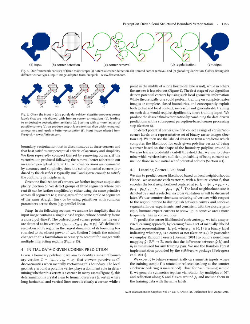
(a) input (b) corner detection (c) corner removal (d) regularization (e) output

Fig. 5. Our framework consists of three major steps: (a) potential corner detection, (b) iterated corner removal, and (c) global regularization. Colors distinguishdifferent curve types. Input image adapted from Freepick – www.flaticon.com.

(a) (b) (c) (d) (e) (f)

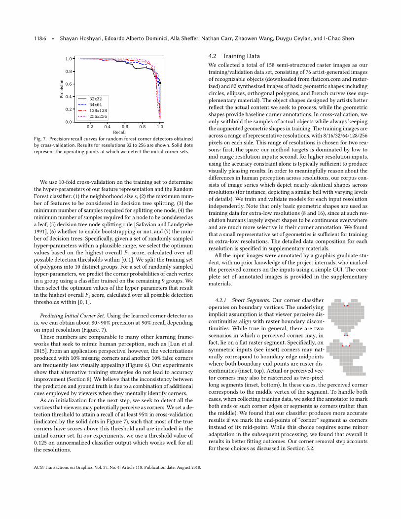
Fig. 6. Given the input in (a), a purely data-driven classifier produces cornerlabels that are misaligned with human corner annotations (b), leadingto undesirable vectorization artifacts (c). Starting with a more lax set ofpossible corners (d), we produce output labels (e) that align with the manualannotations and result in better vectorization (f). Input image adapted fromFreepick – www.flaticon.com.

boundary vectorization that is discontinuous at these corners and

that best satisfies our perceptual criteria of accuracy and simplicity.

We then repeatedly compact this set by removing corners, if the

vectorization produced following the removal better adheres to our

measured perceptual criteria. Our removal decisions are dominated

by accuracy and simplicity, since the set of potential corners pro-

duced by the classifier is typically small and sparse enough to satisfy

the continuity principle as is.

Given the finalized set of corners, we further improve output sim-

plicity (Section 6). We detect groups of fitted segments whose cur-

rent fit can be further simplified by either using the same primitive

across all segments (e.g. using arcs of the same circle or segments

of the same straight line), or by using primitives with common

parameters across them (e.g. parallel lines).

Setup. In the following sections, we assume for simplicity that the

input image contains a single closed region, whose boundary forms

a closed polyline P . The ordered pixel corner points that lie on Pare denoted as its vertices, {p0, . . . ,pm−1,pm = p0}. We define the

resolution of the region as the largest dimension of its bounding box

rounded to the closest power of two. Section 7 details the minimal

changes to this formulation necessary to account for images with

multiple interacting regions (Figure 13).

4 INITIAL DATA-DRIVEN CORNER PREDICTIONGiven a boundary polyline P , we aim to identify a subset of bound-

ary vertices C = {c0, . . . , cn = c0} that viewers perceive as C0

discontinuities when mentally vectorizing this boundary. The local

geometry around a polyline vertex plays a dominant role in deter-

mining whether this vertex is a corner. In many cases (Figure 3), this

determination is crystal clear to human observers (a vertex where

long horizontal and vertical lines meet is clearly a corner, while a

point in the middle of a long horizontal line is not), while in others

the answer is less obvious (Figure 4). The first stage of our algorithm

detects potential corners by using such local geometric information.

While theoretically one could perform training on complete raster

images or complete, closed boundaries, and consequently exploit

both global and local context, successful and generalizable training

on such data would require significantly more training input. We

produce the desired final vectorization by combining the data-driven

predictions with a subsequent perception-based corner processing

step (Section 5).

To detect potential corners, we first collect a range of corner/non-

corner labels on a representative set of binary raster images (Sec-

tion 4.2). We then use the labeled dataset to train a predictor which

computes the likelihood for each given polyline vertex of being

a corner based on the shape of the boundary polyline around it.

We also learn a probability cutoff threshold that we use to deter-

mine which vertices have sufficient probability of being corners; we

include those in our initial set of potential corners (Section 4.1).

4.1 Learning Corner LikelihoodWe aim to predict corner likelihood based on local neighborhoods.

Hence, we associate each vertex pi with a feature vector fi thatencodes the local neighborhood centered at pi : fi = [pi−s − pi , · · · ,pi−1 −pi ,pi+1 −pi , · · · ,pi+s −pi ]

T. The local neighborhood size is

denoted by s and is selected via cross validation as will be discussed

later. We use counter-clockwise ordering of vertices with respect

to the region interior to distinguish between convex and concave

segments. In our experiments, and consistent with the closure prin-

ciple, humans expect corners to show up in concave areas more

frequently than in convex ones.

To predict the corner likelihood of each vertex pi , we take a super-vised learning approach, by learning from a set of manually labeled

feature representations {fi ,yi }, where yi ∈ {0, 1} is a binary label

indicating whether pi is a corner or not (Section 4.2). In particular,

we employ Random Forests [Breiman 2001] to build a non-linear

mapping y : R4s → R, such that the difference between y (fi ) andyi is minimized for any training pair. We use the Random Forest

implementation provided by the scikit-learn package [Pedregosa

et al. 2011].

We expect y to behave symmetrically on symmetric inputs, where

the training sample f is rotated or reflected (as long as the counter

clockwise ordering is maintained). Thus, for each training sample

fi, we generate symmetric replicas via rotation by multiples of 90◦,

and reflection along X and Y axes around pi and include them in

the training data with the same labels.

ACM Transactions on Graphics, Vol. 37, No. 4, Article 118. Publication date: August 2018.

118:6 • Shayan Hoshyari, Edoardo Alberto Dominici, Alla Sheffer, Nathan Carr, Zhaowen Wang, Duygu Ceylan, and I-Chao Shen

0.2 0.4 0.6 0.8 1.0Recall

0.0

0.2

0.4

0.6

0.8

1.0Pr

ecis

ion

32x3264x64128x128256x256

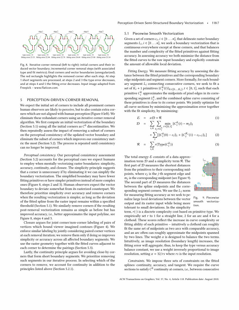
Fig. 7. Precision-recall curves for random forest corner detectors obtainedby cross-validation. Results for resolutions 32 to 256 are shown. Solid dotsrepresent the operating points at which we detect the initial corner sets.

We use 10-fold cross-validation on the training set to determine

the hyper-parameters of our feature representation and the Random

Forest classifier: (1) the neighborhood size s , (2) the maximum num-

ber of features to be considered in decision tree splitting, (3) the

minimum number of samples required for splitting one node, (4) the

minimum number of samples required for a node to be considered as

a leaf, (5) decision tree node splitting rule [Safavian and Landgrebe

1991], (6) whether to enable bootstrapping or not, and (7) the num-

ber of decision trees. Specifically, given a set of randomly sampled

hyper-parameters within a plausible range, we select the optimum

values based on the highest overall F1 score, calculated over all

possible detection thresholds within [0, 1]. We split the training set

of polygons into 10 distinct groups. For a set of randomly sampled

hyper-parameters, we predict the corner probabilities of each vertex

in a group using a classifier trained on the remaining 9 groups. We

then select the optimum values of the hyper-parameters that result

in the highest overall F1 score, calculated over all possible detection

thresholds within [0, 1].

Predicting Initial Corner Set. Using the learned corner detector as

is, we can obtain about 80∼90% precision at 90% recall depending

on input resolution (Figure. 7).

These numbers are comparable to many other learning frame-

works that seek to mimic human perception, such as [Lun et al.

2015]. From an application perspective, however, the vectorizations

produced with 10% missing corners and another 10% false corners

are frequently less visually appealing (Figure 6). Our experiments

show that alternative training strategies do not lead to accuracy

improvement (Section 8). We believe that the inconsistency between

the prediction and ground truth is due to a combination of additional

cues employed by viewers when they mentally identify corners.

As an initialization for the next step, we seek to detect all the

vertices that viewersmay potentially perceive as corners.We set a de-

tection threshold to attain a recall of at least 95% in cross-validation

(indicated by the solid dots in Figure 7), such that most of the true

corners have scores above this threshold and are included in the

initial corner set. In our experiments, we use a threshold value of

0.125 on unnormalized classifier output which works well for all

the resolutions.

4.2 Training DataWe collected a total of 158 semi-structured raster images as our

training/validation data set, consisting of 76 artist-generated images

of recognizable objects (downloaded from flaticon.com and raster-

ized) and 82 synthesized images of basic geometric shapes including

circles, ellipses, orthogonal polygons, and French curves (see sup-

plementary material). The object shapes designed by artists better

reflect the actual content we seek to process, while the geometric

shapes provide baseline corner annotations. In cross-validation, we

only withhold the samples of actual objects while always keeping

the augmented geometric shapes in training. The training images are

across a range of representative resolutions, with 8/16/32/64/128/256

pixels on each side. This range of resolutions is chosen for two rea-

sons: first, the space our method targets is dominated by low to

mid-range resolution inputs; second, for higher resolution inputs,

using the accuracy constraint alone is typically sufficient to produce

visually pleasing results. In order to meaningfully reason about the

differences in human perception across resolutions, our corpus con-

sists of image series which depict nearly-identical shapes across

resolutions (for instance, depicting a similar bell with varying levels

of details). We train and validate models for each input resolution

independently. Note that only basic geometric shapes are used as

training data for extra-low resolutions (8 and 16), since at such res-

olution humans largely expect shapes to be continuous everywhere

and are much more selective in their corner annotation. We found

that a small representative set of geometries is sufficient for training

in extra-low resolutions. The detailed data composition for each

resolution is specified in supplementary materials.

All the input images were annotated by a graphics graduate stu-

dent, with no prior knowledge of the project internals, who marked

the perceived corners on the inputs using a simple GUI. The com-

plete set of annotated images is provided in the supplementary

materials.

4.2.1 Short Segments. Our corner classifieroperates on boundary vertices. The underlying

implicit assumption is that viewer perceive dis-

continuities align with raster boundary discon-

tinuities. While true in general, there are two

scenarios in which a perceived corner may, in

fact, lie on a flat raster segment. Specifically, on

symmetric inputs (see inset) corners may nat-

urally correspond to boundary edge midpoints

where both boundary end-points are raster dis-

continuities (inset, top). Actual or perceived vec-

tor corners may also be rasterized as two-pixel

long segments (inset, bottom). In these cases, the perceived corner

corresponds to the middle vertex of the segment. To handle both

cases, when collecting training data, we asked the annotator to mark

both ends of such corner edges or segments as corners (rather than

the middle). We found that our classifier produces more accurate

results if we mark the end-points of “corner” segment as corners

instead of its mid-point. While this choice requires some minor

adaptation in the subsequent processing, we found that overall it

results in better fitting outcomes. Our corner removal step accounts

for these choices as discussed in Section 5.2.

ACM Transactions on Graphics, Vol. 37, No. 4, Article 118. Publication date: August 2018.

Perception-Driven Semi-Structured Boundary Vectorization • 118:7

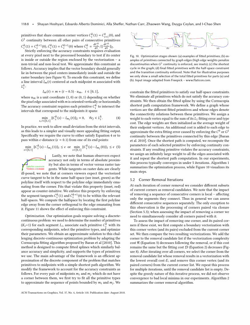
type score: 33fitting error:22.84

type score: 31fitting error:23.80

type score: 32fitting error:22.70

type score: 31fitting error:24.60

type score: 31fitting error:23.54

type score: 31fitting error:23.53

step 1 step 2 step 3 step 4 step 5

Fig. 8. Iterative corner removal (left to right): initial corners and their in-duced vector boundary; incremental corner removal steps (with associatedtype and fit metrics); final corners and vector boundaries (unregularized).The red rectangle highlights the removed corner after each step. At step1 short segments are processed, at steps 2 and 3 the type error decreases,and at steps 4 and 5 the fitting error decreases. Input image adapted fromFreepick – www.flaticon.com.

5 PERCEPTION-DRIVEN CORNER REMOVALWe expect the initial set of corners to include all prominent corners

human observers are likely to perceive, but to also contain extra cor-

ners which are not aligned with human perception (Figure 8 left). We

eliminate these redundant corners using an iterative corner removal

algorithm. We first compute an initial vectorization of the boundary

(Section 5.1) using all the initial corners as C0discontinuities. We

then repeatedly assess the impact of removing a subset of corners

on the perceptual consistency of the updated vector boundary and

eliminate the subset of corners which improves our consistency met-

ric the most (Section 5.2). The process is repeated until consistency

can no longer be improved.

Perceptual consistency. Our perceptual consistency assessment

(Section 5.2) accounts for the perceptual cues we expect humans

to employ when mentally vectorizing raster boundaries: simplicity,

accuracy, continuity, and closure. The simplicity principle suggests

that a corner is unnecessary if by eliminating it we can simplify the

boundary vectorization. The simplified boundary may have fewer

fitting primitives or have simpler primitives instead of more complex

ones (Figure 8, steps 2 and 3). Human observers expect the vector

boundary to deviate somewhat from its rasterized counterpart. We

therefore prioritize simplicity over accuracy and remove corners

when the resulting vectorization is simpler, as long as the deviation

of the fitted spline from the raster input remains within a specified

threshold (Section 5.1). We similarly remove corners if the resulting

post-removal vectorization remains as simple as before but has

improved accuracy, i.e., better approximates the input polyline, see

Figure 8, steps 4 and 5.

Closure argues for joint corner/non-corner labeling of pairs of

vertices which bound viewer imagined contours (Figure 4). We

enforce similar labeling by jointly considering paired corner vertices

at each removal iteration; we remove them only if doing so improves

simplicity or accuracy across all affected boundary segments. We

use the raster geometry together with the fitted curves adjacent to

each corner to determine the pairings (Section 5.3).

Lastly, the continuity principle argues for avoiding close-by cor-

ners that form short boundary segments. We prioritize removing

such segments in our iterative process. In selecting which of the

corners to remove, we account for continuity in addition to the

principles listed above (Section 5.2.1).

5.1 Piecewise Smooth VectorizationGiven a set of corners ci , i ∈ [0 . . .n], that delineate raster boundary

segments Li , i ∈ [0 . . .n], we seek a boundary vectorization that is

continuous everywhere except at these corners, and that balances

the number and complexity of the fitted primitives against fitting

accuracy. In assessing accuracy we both minimize the distance from

the fitted curves to the raw input boundary and explicitly constrain

the amount of allowable local deviation.

Fitting Energy. We measure fitting accuracy by assessing the dis-

tance between the fitted primitives and the corresponding boundary

edge midpoints and segment corners. More formally, for each bound-

ary segment Li connecting consecutive corners, we seek to fit a

set of Ki + 1 primitives {Cki (t )}k ∈[0...Ki ], t ∈ [0, 1], such that each

primitive Cki approximates the midpoints of pixel edges in its corre-

sponding segment Lki , and the combined spline curve consisting of

these primitives is close to its corner points. We jointly optimize for

all curve sections by minimizing the approximation error together

with the fit simplicity, by minimizing:

E = αD + R (1)

D =∑i,k

∑ej ∈Lki

min

t ∈[0,1]

∥Cki (t ) −mj ∥1

+∑i

[∥C0

i (0) − ci ∥1 + ∥CKii (1) − ci+1∥1] (2)

R =∑i,k

r (Type(Cki )) (3)

L0

L1

c0 c1

c2

c3

mj

Im

L2

Fig. 9. Piecewisesmooth vectoriza-tion.

The total energy E consists of a data approx-

imation term D and a simplicity term R. The

first part of D measures the shortest distances

from the primitives to their corresponding mid-

points, where ej is the j-th segment edge and

mj is the corresponding midpoint (see Figure 9).

The second part of D measures the distances

between the spline endpoints and the corre-

sponding segment corners. We use the L1 norm

for measuring fitting accuracy as we seek to pe-

nalize large local deviations between the vector

output and its raster input while being more

tolerant to small deviations. In the simplicity

term, r (·) is a discrete complexity cost based on primitive type. We

empirically set r to 1 for a straight line, 2 for an arc and 4 for a

clothoid. These scores reflect the increase in curve complexity or

fitting ability of each primitive – intuitively a clothoid can roughly

fit the same set of midpoints as two arcs with comparable accuracy,

and an arc often can roughly approximate the midpoints spanned

by two lines. The weight α is designed to balance the two terms.

Intuitively, as image resolution (boundary length) increases, the

fitting error will aggregate; thus, to keep the type versus accuracy

balance constant, we use a weight inversely proportional to image

resolution, setting α = 32/rs where rs is the input resolution.

Constraints. We impose three sets of constraints on the fitted

splines: continuity, accuracy, and tangent. We require the curve

sections to satisfyC0continuity at corners, i.e., between consecutive

ACM Transactions on Graphics, Vol. 37, No. 4, Article 118. Publication date: August 2018.

118:8 • Shayan Hoshyari, Edoardo Alberto Dominici, Alla Sheffer, Nathan Carr, Zhaowen Wang, Duygu Ceylan, and I-Chao Shen

primitives that share common corner vertices Cki (1) = C0

i+1(0), and

G1continuity between all other pairs of consecutive primitives:

Cki (1) = Ck+1

i (0), Cki (1) = Ck+1

i (0) where Cki =dCk

idt /∥

dCki

dt ∥2.Strictly enforcing the accuracy constraints requires evaluation

at every pixel next to the processed boundary to test if its center

is inside or outside the region enclosed by the vectorization – a

non-trivial and non-local test. We approximate this constraint as

follows. Accuracy implies that the vector boundary should generally

lie in-between the pixel centers immediately inside and outside the

raster boundary (see Figure 9). To encode this constraint, we define

a line interval Im (t ) centered at each midpointm associated with

Lki :

Im (t ) =m + (t − 0.5) · um , t ∈ [0, 1],

where um is a unit coordinate (1, 0) or (0, 1) depending on whether

the pixel edge associated withm is oriented vertically or horizontally.

The accuracy constraint requires each primitive Cki to intersect the

intervals that correspond to the midpoints it spans:

min

s,t ∈[0,1]

∥Cki (s ) − Imj (t )∥2 = 0, ∀ej ∈ Lki . (4)

In practice, we seek to allow small deviation from the strict intervals,

as this leads to a simpler and visually more appealing fitting output.

Specifically we require the curve to either satisfy Equation 4 or to

pass within ϵ-distance (ϵ = 0.1) from one of its end points:

min

s ∈[0,1]

∥Cki (s )− Imj (1)∥1 ≤ ϵ or min

s ∈[0,1]

∥Cki (s )− Imj (0)∥1 ≤ ϵ (5)

Satisfies constraintViolates constraint

Lastly, we note that human observers expect

accuracy not only in terms of absolute proxim-

ity but also in terms of vector versus raster tan-

gents. While tangents on raster data are clearly

ill-posed, we note that at corners viewers expect the vectorized

curve tangent to be in the same half-space (see inset, green) as the

polyline itself with respect to the polyline edge immediately ema-

nating from the corner. Fits that violate this property (inset, red)

appear as counter-intuitive. We enforce this property by enforcing

the segment tangents Cki (1) and Ck+1

i (0) to be within the relevant

half-spaces. We compute the halfspace by locating the first polyline

edge away from the corner orthogonal to the edge emanating from

it. Figure 11 shows the effect of enforcing this constraint.

Optimization. Our optimization goals require solving a discrete-

continuous problem: we need to determine the number of primitives

(Ki+1) for each segment Li , associate each primitive Cki with its

corresponding midpoints, select the primitive types, and optimize

their parameters. We obtain an approximate solution to this chal-

lenging discrete-continuous optimization problem by adapting the

Cornucopia fitting algorithm proposed by Baran et al [2010]. This

method is designed to compute fitted splines which similarly bal-

ance accuracy and simplicity, and supports the types of primitives

we use. The main advantage of the framework is an efficient ap-

proximation of the discrete component of the problem that matches

primitives to midpoints with a simple shortest path algorithm. We

modify the framework to account for the accuracy constraints as

follows. For every pair of midpointsmi andmj which do not have

a corner between them, we first try to fit all the primitive types

to approximate the sequence of points bounded bymi andmj . We

(a) (b) (c) (d)

(b-1)

(b-2)

(b-3)

(b-3)

(b-2)

(b-1)

Fig. 10. Optimization stages shown: (a) examples of fitted primitives; (b) ex-amples of primitives connected by graph edges (high edge weights penalizediscontinuities when G1 continuity is enforced, see insets); (c) the shortestcycle in the graph; (d) final fitted primitives with the half-space constraintand the transition continuity enforced. Note that for illustrative purposeswe only show a small selection of the total fitted primitives for parts (a) and(b). Input image adapted from Freepick – www.flaticon.com.

constrain the fitted primitives to satisfy our half-space constraints.

We eliminate all primitives which do not satisfy the accuracy con-

straints. We then obtain the fitted spline by using the Cornucopia

shortest path computation framework. We define a graph whose

vertices are the different fitted primitives and whose edges denote

the connectivity relations between these primitives. We assign a

weight to each vertex equal to the sum of its L1 fitting error and type

cost. The edge weights are then initialized as the average weight of

their endpoint vertices. An additional cost is added to each edge to

approximate the extra fitting error caused by enforcing theC0orG1

continuity between the primitives connected by this edge [Baran

et al. 2010]. Once the shortest path is computed, we recompute the

parameters of each selected primitive by enforcing continuity con-

straints. If any resulting primitive violates the accuracy constraints,

we assign an infinitely large weight to all the edges associated with

it and repeat the shortest path computation. In our experiments,

this process typically converges in under 5 iterations. Algorithm 1

summarizes the optimization process, while Figure 10 visualizes its

main steps.

5.2 Corner Removal IterationsAt each iteration of corner removal we consider different subsets

of current corners as removal candidates. We note that the impact

of removing a sequence of consecutive corners is local – affecting

only the segments they connect. Thus in general we can assess

different consecutive sequences separately. The only exception to

this observation is the processing of corners paired via closure

(Section 5.3); when assessing the impact of removing a corner we

need to simultaneously consider all corners paired with it.

To assess the impact of removing one corner, and its paired cor-

ners if these exist, we first compute a boundary vectorization with

this corner vertex (and its pairs) excluded from the current corner

set. We then compare the two resulting vectorizations. We add the

corner to the removal candidate list if the vectorization complexity

cost R (Equation 3) decreases following the removal, or if this cost

remains the same but the fitting cost D (Equation 2) decreases (Fig-

ure 8). After iterating over all corners, we select the corner from the

removal candidate list whose removal results in a vectorization with

the lowest overall cost E, and remove this corner vertex (and its

paired corners) from the current corner list. We repeat this process

for multiple iterations, until the removal candidate list is empty. De-

spite the greedy nature of this iterative process, we did not observe

convergence to bad local minima in our experiments. Algorithm 2

summarizes the corner removal algorithm.

ACM Transactions on Graphics, Vol. 37, No. 4, Article 118. Publication date: August 2018.

Perception-Driven Semi-Structured Boundary Vectorization • 118:9

5.2.1 Short segments. The set of corners produced by our classi-

fier is typically well-spaced, but can contain some close by corners

— here we consider a pair of corners as close if the distance between

them is shorter than 10% of the image resolution. In general viewers

do not expect to see such short segments in their vectorization as

they violate our expectation of visual continuity. Extra-short seg-

ments with one or two pixels are also a side effect of the discrete

nature of corner detection, and the consequent corner labeling pro-

vided to training which replaces corners visually placed on edges

or flat boundary segments with those nearby non-flat boundary

vertices (Section 4.2.1). We prioritize short segment removal and

attempt to remove such segments before executing the main loop.

We only consider segments that in the current vectorization are

fit with individual line primitives, as we expect any higher com-

plexity primitive to reflect actual necessary geometry. We measure

the angles at the ends of the line primitive fitted ϕ1 and ϕ2. We

use these angles to asses if the primitive should be treated as sym-

metric or not, and classify it as symmetric if |ϕ1 − ϕ2 | < 2◦. For

non-symmetric primitives, we first apply the default removal test

based on simplicity and accuracy, and remove the corner which

improves R the most. If neither corner is removed, we remove the

corner with the more obtuse angle, if that angle is above 120◦and

R increases by less than 1 (i.e. conceptually we replace a line by an

arc). If one corner is convex and one concave, we only consider the

convex one. For symmetric primitives, if the cost R improves by

removing both corners or if both angles are above 120◦and the cost

increase is less than 1 we remove both.

For length one segments we simply replace the two corners with

one mid-edge corner. For length two segments we apply the same

method but with relaxed thresholds, we classify the primitive as

symmetric if |ϕ1 − ϕ2 | < 15◦and use an angle threshold of 100

◦

instead of 120◦. In addition, for primitives deemed symetric we asses

the cost of moving the corner to the middle, and perform this move

if the cost improves. Figure 11 shows the effect of this process.

input no half-space no short segments with all features

Fig. 11. Effect of the half-space constraint and the short segement precess-ing step. Input image adapted from Freepick – www.flaticon.com.

5.3 Computing Global Context CuesThere are multiple standard methods for the convex partitioning

of closed curves, e.g. [Lien and Amato 2004]. However, none are

applicable to raster boundaries where the question of how to de-

fine convexity even on simple shapes (see circle in Figure 3) is not

evident. We use two criteria to identify pairs of concave corner

vertices that viewers are likely to perceive as connected following

the closure principle (Figure 4). First we look for pairs of corner

points which are closest vis-a-vis the model medial axis, i.e., ones

with a common circle that touches both points and is entirely in-

side the processed region. We use a scaled version (by a factor of

0.90) of the common circle for the inside test to handle the inaccu-

racy inherent to raster data. We augment this test with a second

closure test designed for corners which are visually paired due to

local geometry but not necessarily closest vis-a-vis the medial axis.

This test is motivated by the continuation princi-

ple that suggests that viewers similarly partition

shapes along invisible contours when these contours

smoothly extend the outer contour (see inset). We

apply this test to pairs of concave points that are

internally visible from one another, i.e., ones that

can potentially define an imaginary internal contour

that partitions the shape. We pair the points if the

angles between the line connecting the tangents of the fitted splines

on the left or right of them are under 5◦.

input unregularized regularized

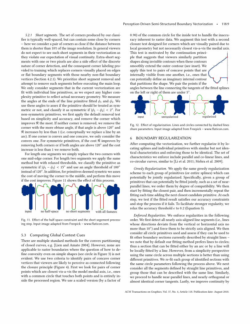
Fig. 12. Effect of regularization. Lines and circles connected by dashed linesshare parameters. Input image adapted from Freepick – www.flaticon.com.

6 BOUNDARY REGULARIZATIONAfter computing the vectorization, we further regularize it by lo-

cating splines and individual primitives with similar but not iden-

tical characteristics and enforcing those to be identical. The set of

characteristics we enforce include parallel and co-linear lines, and

co-circular curves, similar to [Li et al. 2011; Mehra et al. 2009].

Greedy Regularization. We apply the same greedy regularization

scheme to each group of primitives (or entire splines) which can

potentially be jointly regularized. Specifically, given a group of

primitives that can potentially be fitted jointly, such as a set of near-

parallel lines, we order them by degree of compatibility. We then

start by fitting the closest pair, and then incrementally repeat the

fitting each time adding the next closest candidate primitive. At each

step, we test if the fitted result satisfies our accuracy constraints

and stop the process if it fails. To facilitate stronger regularity, we

relax the accuracy threshold ϵ to 0.2 (Equation 5).

Enforced Regularities. We enforce regularities in the following

order. We first detect all nearly axis-aligned line segments (i.e., lines

whose directions deviate from the vertical or horizontal axis no

more than 10◦) and force them to be strictly axis aligned. We then

consider all circle primitives used and assess if they can be used to

fit other boundary sections currently described by straight lines –

we note that by default our fitting method prefers lines to circles;

thus a section that can be fitted either by an arc or by a line will

be locally fitted by a line. However, from a simplicity perspective

using the same circle across multiple sections is better than using

different primitives. We re-fit each group of identified sections with

the same circle parameters following the process above. We next

consider all the segments defined by straight line primitives, and

group those that can be described with the same line. Similarly,

we proceed to handle near-parallel lines, and nearly orthogonal or

almost identical corner tangents. Lastly, we improve continuity by

ACM Transactions on Graphics, Vol. 37, No. 4, Article 118. Publication date: August 2018.

118:10 • Shayan Hoshyari, Edoardo Alberto Dominici, Alla Sheffer, Nathan Carr, Zhaowen Wang, Duygu Ceylan, and I-Chao Shen

considering corners with nearly identical tangents on either side

and re-fitting them using a continuous vector spline. In our angle

computation, we consider tangents to be nearly identical if they

are within an angle difference of 20◦, a threshold at which humans

perceive two connecting curves with corresponding tangent angle

as continuous [Hess and Field 1999]. Figure 12 shows the before

and after regularization results.

7 MULTI-COLOR INPUTSHandling of multi-color inputs raises a few questions not addressed

by the single boundary setup. First, we need to resolve topological

ambiguities at corners [Kopf and Lischinski 2011]. We use the frame-

work by Kopf et al. for this task. We also use their framework to

extract the region boundary graph. Edges in this graph correspond

to raster boundary segments shared by two regions and vertices

correspond to raster boundary vertices shared by three or four re-

gions. Our second task is to determine the location of corners along

the boundaries. We use our corner detector trained at the closest

power of two resolution to find the corner probabilities for each

region boundary independently. We classify vertices along segments

shared by two regions as corners if it is deemed as a corner with

respect to both regions (we prefer to err on the side of more con-

tinuous solutions as viewers are more sensitive to redundant than

to missing corners). Lastly we seek to determine the continuity at

boundary vertices adjacent to multiple regions. We note that with

accuracy constraints in place at vertices adjacent to three regions

we can at most enforce one boundary to be continuous. At valence

four vertices two crossing boundaries can be also be continuous. We

determine which continuity constraints to enforce as follows. If a

multi-region vertex is considered a C0corner by all the boundaries,

or all but one we use this classification as is. Similarly if a vertex

has a corner vertex within one pixel distance on any boundary, we

classify it as a corner with respect to that boundary. We resolve

conflicts, where two or more boundaries have the vertex marked as

non-corner using angles. Specifically we vectorize the conflicting

regions independently, treating this vertex as corner on all. We then

measure the angles between the tangents at this vertex and greedily

mark the boundary with the most obtuse angle as the continuous

one, and mark the vertex as a corner for the rest.

All resulting boundary segments are then fitted individually us-

ing a similar pipeline as the single color. The resulting vectorized

boundary segments are not guaranteed to be connected. Our final

step connects all segments by performing an additional global fitting

step with positional constraints for the segment endpoints. If all

segments meeting at a shared multi-region vertex areC0continuous

at it, we simply constrain their end vertices to the average of their

current positions. If one segment is G1continuous, we average end

vertex positions of the other segments and project this average to

the curve. We then refit the curves with this positional constraint.

8 RESULTS AND VALIDATIONWe tested our method on a large set of close to 200 images, at differ-

ent pixel resolutions ranging in size from 16×16 to 256×256; we also

tested a range of multi-color inputs with region sizes as small as 2×2.

We show a range of representative results throughout the paper (see

e.g. Figures 15, 16) and provide numerous additional results in the

supplementary material. As our work focuses on boundary vector-

ization, our test sets are dominated by images that consist of two

regions separated by a single closed boundary. While these inputs

best illustrate the impact of our algorithmic choices, we also include

various multi-region and multi-color examples (Figures 1, 13). Our

results look consistent with human expectations across the board.

Besides visual inspection, we also perform a thorough evaluation

by comparing our method to artist created results and algorithmic

alternatives.

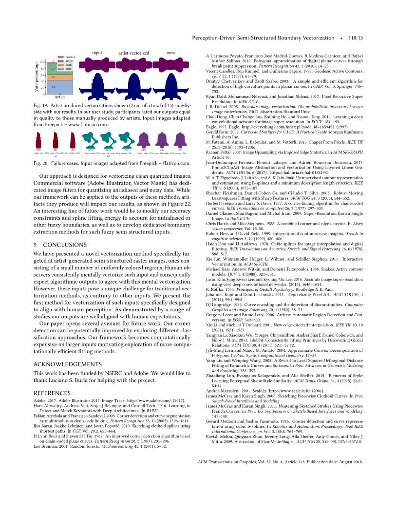
Perceptual Ground Truth Comparison. We asked an artist to man-

ually vectorize 15 representative inputs. Figure 19 shows 2 of these

artist produced vectorizations side-by-side with our results. Addi-

tional results are included in the supplementary material. While it

took the artists on average 30 to 45 minutes to generate each exam-

ple vectorization, our method automatically produces qualitatively

similar results in a fraction of this time.

Algorithmic Alternatives. We also compared our results to those

generated by a range of available methods. We compared our results

to three publicly available vectorizationmethods: Adobe Trace [Adobe

2017], Vector Magic [Vector Magic 2017] and Potrace [Selinger 2003].

Additionally, we tested against state-of-the-art upscaling [Stepin

2003] and super-resolution [Wang et al. 2015] methods. Lastly, we

compared against the polyline fitting method of [Baran et al. 2010].

Since this method fits a piecewise smooth curve to a polyline, we

used boundary midpoints as input polyline vertices. In all cases, we

adjusted method parameters to produce results that most closely

resemble human expectations. For these comparisons, we focus on

input resolutions of up to 128 and show representative examples at

resolutions 32, 64 and 128 in Figure 15. We observe that, at higher

resolutions, fitting accuracy dominates all other cues with all fit-

ting and vectorization methods producing similar results. The small

components of multi-region examples (as shown in Figure 1 and the

supplementary material) implicitly provide examples of lower reso-

lution input, and our method produces outputs that are significantly

more consistent with viewer expectations for these regions.

While we fundamentally focus on a different problem, we also

provide comparisons to the method of Kopf et al. [2011] in Figures

17 and 18. Kopf et al. focus on resolving topological ambiguities be-

tween multiple regions that touch at a pixel corner, and use standard

spline fitting once these ambiguities are fixed. In contrast, we focus

on vectorization of semi-structured region boundaries. While many

of the inputs shown by Kopf et. al. have irregularly shaped regions

only a few pixels large, we typically focus on resolutions where

region shape or structure is more pronounced. On such inputs, our

methods outperforms the method of Kopf et al. [2011], see Figure 17.

Small (1-2 pixel wide) irregularly shaped regions are best fitted using

simple splines rather than our framework (see Figure 18).

Lastly, we compare the results of our complete algorithm to those

produced using the learned classifier alone, without the progressive

corner removal (Figures 6 and 14).

Qualitative Evaluation. To further confirm that our results are

well aligned with human expectation, we conducted a comparative

user study. For each question, we showed participants the input,

our result, and one of the algorithmic alternatives side by side. We

then asked them to select the result that resembles the input the

ACM Transactions on Graphics, Vol. 37, No. 4, Article 118. Publication date: August 2018.

Perception-Driven Semi-Structured Boundary Vectorization • 118:11

Potrace oursinput Adobe Trace Vector Magic Potrace oursinput Adobe Trace Vector Magic

Fig. 13. Vectorization of multi-color inputs. Dog and rooster images © Twitter, Inc.

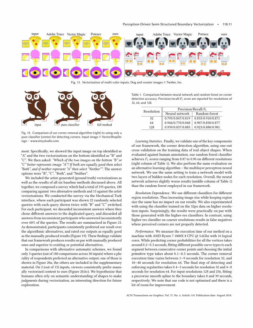
pure classifier full methodinput

Fig. 14. Comparison of our corner removal algorithm (right) to using only apure classifier (center) for detecting corners. Input image © VectorShopDe-sign – www.etsystudio.com.

most. Specifically, we showed the input image on top identified as

“A” and the two vectorizations on the bottom identified as “B” and

“C”. We then asked: “Which of the two images on the bottom “B” or“C” better represents image “A”? If both are equally good then select“Both”, and if neither represent “A” then select “Neither””. The answeroptions were “B”, “C”, “Both”, and “Neither”.

We included the artist-generated (ground truth) vectorizations as

well as the results of all six baseline methods discussed above. All

together, we composed a survey which had a total of 195 queries, 180

comparing against two alternative methods and 15 against the artist

vectorizations. We conducted the survey via the Mechanical Turk

interface, where each participant was shown 22 randomly selected

queries with each query shown twice with “B” and “C” switched.

For each participant, we discarded inconsistent answers where they

chose different answers to the duplicated query, and discarded all

answers from inconsistent participants who answered inconsistently

over 60% of the queries. The results are summarized in Figure 21.

As demonstrated, participants consistently preferred our result over

the algorithmic alternatives, and rated our outputs as equally good

as the manually produced results (Figure 19). These findings validate

that our framework produces results on par with manually produced

ones and superior to existing or potential alternatives.

In comparisons with alternative automatic schemes, we found

only 3 queries (out of 180 comparisons across 30 inputs) where a plu-

rality of respondents preferred an alternative output; one of those is

shown in Figure 20a, the others are included in the supplementary

material. On 2 (out of 15) inputs, viewers consistently prefer manu-

ally vectorized content to ours (Figure 20,bc). We hypothesize that

humans often rely on semantic understanding of shapes to make

judgments during vectorization, an interesting direction for future

exploration.

Table 1. Comparison between neural network and random forest on cornerdetection accuracy. Precision/recall/F1 score are reported for resolutions of32, 64, and 128.

Resolution

Precision/Recall/F1

Neural network Random forest

32 0.793/0.847/0.819 0.835/0.910/0.871

64 0.944/0.770/0.848 0.907/0.850/0.877

128 0.939/0.837/0.885 0.923/0.880/0.901

Learning Statistics. Finally, we validate one of the key components

of our framework, the corner detection algorithm, using one-out

cross validation on the training data of real object shapes. When

evaluated against human annotation, our random forest classifier

achieves F1 scores ranging from 0.87 to 0.90 on different resolutions

(right column of Table 1). We also perform the same evaluation on

an alternative learning algorithm – the multilayer perceptron neural

network. We use the same setting to train a network model with

two layers of hidden nodes for each resolution. Overall, the neural

network achieves slightly worse results (middle column of Table 1)

than the random forest employed in our framework.

Resolution Dependence. We use different classifiers for different

region resolutions. Thus increasing image size while keeping region

size the same has no impact on our results. We also experimented

with using the classifier trained on the 32px data on higher resolu-

tion inputs. Surprisingly, the results were practically on par with

those generated with the higher-res classifiers. In contrast, using

higher-res classifier on coarser resolutions results in false negatives

where perceived corners are not properly detected.

Performance. We measure the execution time of our method on a

machine with AMD Ryzen 7 1800X 8 CPU @ 3.6Ghz with 16 logical

cores. While predicting corner probabilities for all the vertices takes

around 0.2−0.3 seconds, fitting different possible curve types to eachsegment between consecutive corner points and choosing the initial

primitive type takes about 0.1−0.5 seconds. The corner removal

execution time varies between 1−9 seconds for resolution 32, and

10−40 seconds for resolution 64. The final step of detecting and

enforcing regularities takes 0.4−3 seconds for resolution 32 and 4−8

seconds for resolution 64. For input resolutions 128 and 256, fitting

a piecewise smooth spline to the boundary takes 8 and 39 seconds,

respectively. We note that our code is not optimized and there is a

lot of room for improvement.

ACM Transactions on Graphics, Vol. 37, No. 4, Article 118. Publication date: August 2018.

118:12 • Shayan Hoshyari, Edoardo Alberto Dominici, Alla Sheffer, Nathan Carr, Zhaowen Wang, Duygu Ceylan, and I-Chao Shen

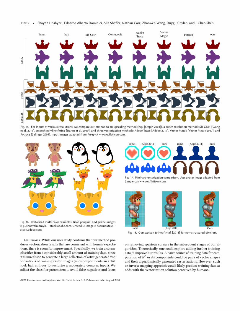
input hqx SR-CNN CornucopiaAdobeTrace

VectorMagic Potrace ours

32x32

64x64

128x128

Fig. 15. For inputs at various resolutions, we compare out method to an upscaling method (hqx [Stepin 2003]), a super-resolution method (SR-CNN [Wanget al. 2015], smooth polyline fitting [Baran et al. 2010], and three vectorization methods: Adobe Trace [Adobe 2017], Vector Magic [Vector Magic 2017], andPotrace [Selinger 2003]. Input images adapted from Freepick – www.flaticon.com.

Fig. 16. Vectorized multi-color examples. Bear, penguin, and giraffe images© pushnovaliudmyla – stock.adobe.com. Crocodile image ©MarinaMays –stock.adobe.com.

Limitations. While our user study confirms that our method pro-

duces vectorization results that are consistent with human expecta-

tions, there is room for improvement. Specifically, we train a corner

classifier from a considerably small amount of training data, since

it is unrealistic to generate a large collection of artist generated vec-

torizations of training raster images (in our experiments an artist

took half an hour to vectorize a moderately complex input). We

adjust the classifier parameters to avoid false negatives and focus

input [Kopf 2011]us

ours input [Kopf 2011] ours

Fig. 17. Pixel-art vectorization comparison. User avatar image adapted fromSimpleIcon – www.flaticon.com.

Input [Kopf 2011] OursFig. 18. Comparison to Kopf et al. [2011] for non-structured pixel-art.

on removing spurious corners in the subsequent stages of our al-

gorithm. Theoretically, one could explore adding further training

data to improve our results. A naïve source of training data for com-

putation of RP or its components could be pairs of vector shapes

and their algorithmically generated rasterizations. However, such

an inverse mapping approach would likely produce training data at

odds with the vectorization solution perceived by humans.

ACM Transactions on Graphics, Vol. 37, No. 4, Article 118. Publication date: August 2018.

Perception-Driven Semi-Structured Boundary Vectorization • 118:13

input artist vectorized ours

Fig. 19. Artist produced vectorizations shown (2 out of a total of 15) side-by-side with our results. In our user study, participants rated our outputs equalin quality to those manually produced by artists. Input images adaptedfrom Freepick – www.flaticon.com.

artist artistours oursourshqxinput input input

(a) (b) (c)Votes artist: 57% ours: 25% both: 11% neither: 7% Votes artist: 75% ours: 7% both: 11% neither: 7% Votes hqx: 75% ours: 7% both: 3% neither: 15%

Fig. 20. Failure cases. Input images adapted from Freepick – flaticon.com.

Our approach is designed for vectorizing clean quantized images.

Commercial software (Adobe Illustrator, Vector Magic) has dedi-

cated image filters for quantizing antialiased and noisy data. While

our framework can be applied to the outputs of these methods, arti-

facts they produce will impact our results, as shown in Figure 22.

An interesting line of future work would be to modify our accuracy

constraints and spline fitting energy to account for antialiased or

other fuzzy boundaries, as well as to develop dedicated boundary

extraction methods for such fuzzy semi-structured inputs.

9 CONCLUSIONSWe have presented a novel vectorization method specifically tar-

geted at artist-generated semi-structured raster images, ones con-

sisting of a small number of uniformly colored regions. Human ob-

servers consistently mentally vectorize such input and consequently

expect algorithmic outputs to agree with this mental vectorization.

However, these inputs pose a unique challenge for traditional vec-

torization methods, as contrary to other inputs. We present the

first method for vectorization of such inputs specifically designed

to align with human perception. As demonstrated by a range of

studies our outputs are well aligned with human expectations.

Our paper opens several avenues for future work. Our corner

detection can be potentially improved by exploring different clas-

sification approaches. Our framework becomes computationally

expensive on larger inputs motivating exploration of more compu-

tationally efficient fitting methods.

ACKNOWLEDGEMENTSThis work has been funded by NSERC and Adobe. We would like to

thank Luciano S. Burla for helping with the project.

REFERENCESAdobe. 2017. Adobe Illustrator 2017: Image Trace. http://www.adobe.com/. (2017).

Hani Altwaijry, Andreas Veit, Serge J Belongie, and Cornell Tech. 2016. Learning to

Detect and Match Keypoints with Deep Architectures.. In BMVC.FabiánArrebola and Francisco Sandoval. 2005. Corner detection and curve segmentation

by multiresolution chain-code linking. Pattern Recognition 38, 10 (2005), 1596–1614.

Ilya Baran, Jaakko Lehtinen, and Jovan Popović. 2010. Sketching clothoid splines using

shortest paths. In CGF, Vol. 29,2. 655–664.H Lynn Beus and Steven SH Tiu. 1987. An improved corner detection algorithm based

on chain-coded plane curves. Pattern Recognition 20, 3 (1987), 291–296.

Leo Breiman. 2001. Random forests. Machine learning 45, 1 (2001), 5–32.

A Carmona-Poyato, Francisco José Madrid-Cuevas, R Medina-Carnicer, and Rafael

Muñoz-Salinas. 2010. Polygonal approximation of digital planar curves through

break point suppression. Pattern Recognition 43, 1 (2010), 14–25.

Vicent Caselles, Ron Kimmel, and Guillermo Sapiro. 1997. Geodesic Active Contours.

IJCV 22, 1 (1997), 61–79.

Dmitry Chetverikov and Zsolt Szabo. 2003. A simple and efficient algorithm for

detection of high curvature points in planar curves. In CAIP, Vol. 3. Springer, 746–753.

Ryan Dahl, Mohammad Norouzi, and Jonathan Shlens. 2017. Pixel Recursive Super

Resolution. In IEEE ICCV.J. R. Diebel. 2008. Bayesian image vectorization: The probabilistic inversion of vector

image rasterization. Ph.D. dissertation, Stanford Univ.

Chao Dong, Chen Change Loy, Kaiming He, and Xiaoou Tang. 2014. Learning a deep

convolutional network for image super-resolution. In ECCV. 184–199.Eagle. 1997. Eagle. http://everything2.com/index.pl?node_id=1859453. (1997).

Gerald Farin. 2002. Curves and Surfaces for CAGD: A Practical Guide. Morgan Kaufmann

Publishers Inc.

M. Fatemi, A. Amini, L. Baboulaz, and M. Vetterli. 2016. Shapes From Pixels. IEEE TIP25, 3 (2016), 1193–1206.

Raanan Fattal. 2007. Image Upsampling via Imposed Edge Statistics. In ACM SIGGRAPH.Article 95.

Jean-Dominique Favreau, Florent Lafarge, and Adrien Bousseau Bousseau. 2017.

Photo2ClipArt: Image Abstraction and Vectorization Using Layered Linear Gra-

dients. ACM TOG 36, 6 (2017). https://hal.inria.fr/hal-01581981

M. A. T. Figueiredo, J. LeitÃčo, andA. K. Jain. 2000. Unsupervised contour representation

and estimation using B-splines and a minimum description length criterion. IEEETIP 9, 6 (2000), 1075–187.

Shachar Fleishman, Daniel Cohen-Or, and Cláudio T. Silva. 2005. Robust Moving

Least-squares Fitting with Sharp Features. ACM TOG 24, 3 (2005), 544–552.

Herbert Freeman and Larry S. Davis. 1977. A corner-finding algorithm for chain-coded

curves. IEEE Transactions on computers 26, 3 (1977), 297–303.Daniel Glasner, Shai Bagon, and Michal Irani. 2009. Super-Resolution from a Single

Image. In IEEE ICCV.Chris Harris and Mike Stephens. 1988. A combined corner and edge detector.. In Alvey

vision conference, Vol. 15. 50.Robert Hess and David Field. 1999. Integration of contours: new insights. Trends in

cognitive sciences 3, 12 (1999), 480–486.Hsieh Hou and H Andrews. 1978. Cubic splines for image interpolation and digital

filtering. IEEE Transactions on Acoustics, Speech, and Signal Processing 26, 6 (1978),

508–517.

Xie Jun, Winnemöller Holger, Li Wilmot, and Schiller Stephen. 2017. Interactive

Vectorization. In ACM SIGCHI.Michael Kass, Andrew Witkin, and Demetri Terzopoulos. 1988. Snakes: Active contour

models. IJCV 1, 4 (1988), 321–331.

Jiwon Kim, Jung Kwon Lee, and Kyoung Mu Lee. 2016. Accurate image super-resolution

using very deep convolutional networks. (2016), 1646–1654.

K. Koffka. 1955. Principles of Gestalt Psychology. Routledge & K. Paul.

Johannes Kopf and Dani Lischinski. 2011. Depixelizing Pixel Art. ACM TOG 30, 4

(2011), 99:1–99:8.

DJ Langridge. 1982. Curve encoding and the detection of discontinuities. ComputerGraphics and Image Processing 20, 1 (1982), 58–71.

Gregory Lecot and Bruno Levy. 2006. Ardeco: Automatic Region Detection and Con-

version. In EGSR. 349–360.Xin Li and Michael T Orchard. 2001. New edge-directed interpolation. IEEE TIP 10, 10

(2001), 1521–1527.

Yangyan Li, Xiaokun Wu, Yiorgos Chrysanthou, Andrei Sharf, Daniel Cohen-Or, and

Niloy J. Mitra. 2011. GlobFit: Consistently Fitting Primitives by Discovering Global

Relations. ACM TOG 30, 4 (2011), 52:1–52:12.

Jyh-Ming Lien and Nancy M. Amato. 2004. Approximate Convex Decomposition of

Polygons. In Proc. Symp. Computational Geometry. 17–26.Yang Liu and Wenping Wang. 2008. A Revisit to Least Squares Orthogonal Distance

Fitting of Parametric Curves and Surfaces. In Proc. Advances in Geometric Modelingand Processing. 384–397.

Zhaoliang Lun, Evangelos Kalogerakis, and Alla Sheffer. 2015. Elements of Style:

Learning Perceptual Shape Style Similarity. ACM Trans. Graph. 34, 4 (2015), 84:1–84:14.

Andrea Mazzoleni. 2001. Scale2x. http://www.scale2x.it/. (2001).

James McCrae and Karan Singh. 2008. Sketching Piecewise Clothoid Curves. In Proc.Sketch-Based Interfaces and Modeling.

James McCrae and Karan Singh. 2011. Neatening Sketched Strokes Using Piecewise

French Curves. In Proc. EG Symposium on Sketch-Based Interfaces and Modeling.141–148.

Gerard Medioni and Yoshio Yasumoto. 1986. Corner detection and curve represen-

tation using cubic B-splines. In Robotics and Automation. Proceedings. 1986 IEEEInternational Conference on, Vol. 3. IEEE, 764–769.

Ravish Mehra, Qingnan Zhou, Jeremy Long, Alla Sheffer, Amy Gooch, and Niloy J.

Mitra. 2009. Abstraction of Man-Made Shapes. ACM TOG 28, 5 (2009), 137:1–137:10.

ACM Transactions on Graphics, Vol. 37, No. 4, Article 118. Publication date: August 2018.

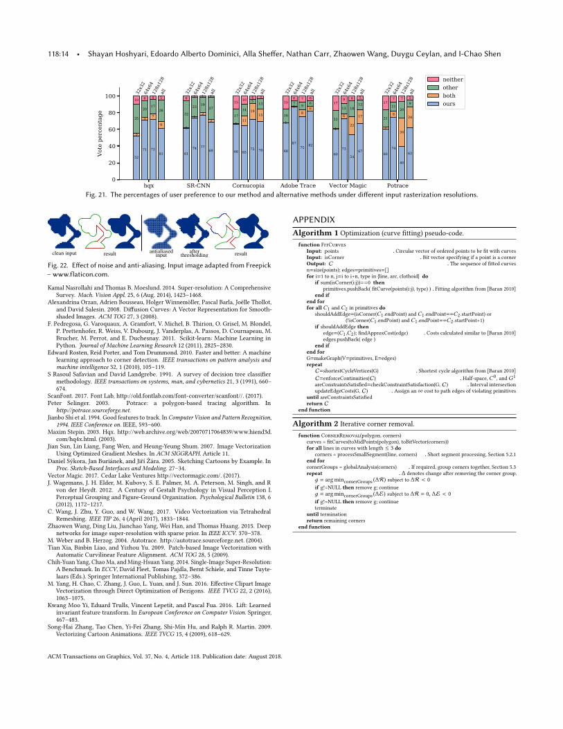
118:14 • Shayan Hoshyari, Edoardo Alberto Dominici, Alla Sheffer, Nathan Carr, Zhaowen Wang, Duygu Ceylan, and I-Chao Shen

hqx SR-CNN Cornucopia Adobe Trace Vector Magic Potrace0

20

40

60

80

100Vo

te p

erce

ntag

e

52

3

35

10

71

3

20

6

72

7

17

4

61

9

26

5

32x3

264

x64

128x

128

all

61

1

32

6

74

1

23

2

77

3

19

1

69

3

27

1

32x3

264

x64

128x

128

all

66

1

17

15

65

11

14

10

72

19

54

70

15

13

3

32x3

264

x64

128x

128

all

68

1

16

15

87

176

75

8

9

7

82

666

32x3

264

x64

128x

128

all

60

1

22

17

73

6

13

9

54

22

18

6

67

17

12

5

32x3

264

x64

128x

128

all

60

2

21

17

74

8

11

7

40

34

20

7

62

24

95

32x3

264

x64

128x

128

all

neitherotherbothours

Fig. 21. The percentages of user preference to our method and alternative methods under different input rasterization resolutions.

antialiasedinput

after thresholding resultclean input result

Fig. 22. Effect of noise and anti-aliasing. Input image adapted from Freepick– www.flaticon.com.

Kamal Nasrollahi and Thomas B. Moeslund. 2014. Super-resolution: A Comprehensive

Survey. Mach. Vision Appl. 25, 6 (Aug. 2014), 1423–1468.Alexandrina Orzan, Adrien Bousseau, Holger Winnemöller, Pascal Barla, Joëlle Thollot,

and David Salesin. 2008. Diffusion Curves: A Vector Representation for Smooth-

shaded Images. ACM TOG 27, 3 (2008).

F. Pedregosa, G. Varoquaux, A. Gramfort, V. Michel, B. Thirion, O. Grisel, M. Blondel,

P. Prettenhofer, R. Weiss, V. Dubourg, J. Vanderplas, A. Passos, D. Cournapeau, M.

Brucher, M. Perrot, and E. Duchesnay. 2011. Scikit-learn: Machine Learning in

Python. Journal of Machine Learning Research 12 (2011), 2825–2830.

Edward Rosten, Reid Porter, and Tom Drummond. 2010. Faster and better: A machine

learning approach to corner detection. IEEE transactions on pattern analysis andmachine intelligence 32, 1 (2010), 105–119.

S Rasoul Safavian and David Landgrebe. 1991. A survey of decision tree classifier

methodology. IEEE transactions on systems, man, and cybernetics 21, 3 (1991), 660–674.

ScanFont. 2017. Font Lab, http://old.fontlab.com/font-converter/scanfont//. (2017).

Peter Selinger. 2003. Potrace: a polygon-based tracing algorithm. In

http://potrace.sourceforge.net.Jianbo Shi et al. 1994. Good features to track. In Computer Vision and Pattern Recognition,

1994. IEEE Conference on. IEEE, 593–600.Maxim Stepin. 2003. Hqx. http://web.archive.org/web/20070717064839/www.hiend3d.

com/hq4x.html. (2003).

Jian Sun, Lin Liang, Fang Wen, and Heung-Yeung Shum. 2007. Image Vectorization

Using Optimized Gradient Meshes. In ACM SIGGRAPH. Article 11.Daniel Sýkora, Jan Buriánek, and Jiří Žára. 2005. Sketching Cartoons by Example. In

Proc. Sketch-Based Interfaces and Modeling. 27–34.Vector Magic. 2017. Cedar Lake Ventures http://vectormagic.com/. (2017).

J. Wagemans, J. H. Elder, M. Kubovy, S. E. Palmer, M. A. Peterson, M. Singh, and R

von der Heydt. 2012. A Century of Gestalt Psychology in Visual Perception I.

Perceptual Grouping and Figure-Ground Organization. Psychological Bulletin 138, 6

(2012), 1172–1217.

C. Wang, J. Zhu, Y. Guo, and W. Wang. 2017. Video Vectorization via Tetrahedral

Remeshing. IEEE TIP 26, 4 (April 2017), 1833–1844.

Zhaowen Wang, Ding Liu, Jianchao Yang, Wei Han, and Thomas Huang. 2015. Deep

networks for image super-resolution with sparse prior. In IEEE ICCV. 370–378.M. Weber and B. Herzog. 2004. Autotrace. http://autotrace.sourceforge.net. (2004).

Tian Xia, Binbin Liao, and Yizhou Yu. 2009. Patch-based Image Vectorization with

Automatic Curvilinear Feature Alignment. ACM TOG 28, 5 (2009).

Chih-Yuan Yang, ChaoMa, andMing-Hsuan Yang. 2014. Single-Image Super-Resolution:

A Benchmark. In ECCV, David Fleet, Tomas Pajdla, Bernt Schiele, and Tinne Tuyte-

laars (Eds.). Springer International Publishing, 372–386.

M. Yang, H. Chao, C. Zhang, J. Guo, L. Yuan, and J. Sun. 2016. Effective Clipart Image

Vectorization through Direct Optimization of Bezigons. IEEE TVCG 22, 2 (2016),

1063–1075.

Kwang Moo Yi, Eduard Trulls, Vincent Lepetit, and Pascal Fua. 2016. Lift: Learned

invariant feature transform. In European Conference on Computer Vision. Springer,467–483.

Song-Hai Zhang, Tao Chen, Yi-Fei Zhang, Shi-Min Hu, and Ralph R. Martin. 2009.

Vectorizing Cartoon Animations. IEEE TVCG 15, 4 (2009), 618–629.

APPENDIXAlgorithm 1 Optimization (curve fitting) pseudo-code.

function FitCurves

Input: points ▷Circular vector of ordered points to be fit with curves

Input: isCorner ▷Bit vector specifying if a point is a corner

Output: C ▷The sequence of fitted curves

n=size(points); edges=primitives=[]for i=1 to n, j=i to i+n, type in {line, arc, clothoid} do

if sum(isCorner(i:j))==0 thenprimitives.pushBack( fitCurve(points(i:j), type) ) ▷Fitting algorithm from [Baran 2010]

end ifend forfor allC1 andC2 in primitives do

shouldAddEdge=(isCorner(C1 .endPoint) andC1 .endPoint==C2 .startPoint) or

(!isCorner(C1 .endPoint) andC1 .endPoint==C2 .startPoint+1)

if shouldAddEdge thenedge=(C1 ,C2); findApproxCost(edge) ▷Costs calculated similar to [Baran 2010]

edges.pushBack( edge )

end ifend forG=makeGraph(V=primitives, E=edges)repeatC=shortestCycleVertices(G) ▷Shortest cycle algorithm from [Baran 2010]

C=enforceContinuities(C) ▷Half-space,C0, andG1

areConstraintsSatisfied=checkConstraintSatisfaction(G, C) ▷Interval intersectionupdateEdgeCosts(G, C) ▷Assign an∞ cost to path edges of violating primitives

until areConstraintsSatisfiedreturn C

end function

Algorithm 2 Iterative corner removal.

function CornerRemoval(polygon, corners)

curves = fitCurves(toMidPoints(polygon), toBitVector(corners))

for all lines in curves with length ≤ 3 docorners = processSmallSegment(line, corners) ▷Short segment processing, Section 5.2.1

end forcornerGroups = globalAnalysis(corners) ▷If required, group corners together, Section 5.3

repeat ▷∆ denotes change after removing the corner group.

д = arg mincornerGroups

(∆R ) subject to ∆R < 0

if g!=NULL then remove g; continue

д = arg mincornerGroups

(∆E) subject to ∆R = 0, ∆E < 0

if g!=NULL then remove g; continue

terminate

until termination

return remaining corners

end function

ACM Transactions on Graphics, Vol. 37, No. 4, Article 118. Publication date: August 2018.