Perception-Based Contrast Enhancement of Imagesmajumder/docs/TAP07.pdf · Perception-Based Contrast Enhancement of Images • Article 17 / 3 the local contrast C are related by ∂C

17

Perception-Based Contrast Enhancement of Images

ADITI MAJUMDER and SANDY IRANI

University of California, Irvine

Study of contrast sensitivity of the human eye shows that our suprathreshold contrast sensitivity follows the Weber Law and,

hence, increases proportionally with the increase in the mean local luminance. In this paper, we effectively apply this fact to

design a contrast-enhancement method for images that improves the local image contrast by controlling the local image gradient

with a single parameter. Unlike previous methods, we achieve this without explicit segmentation of the image, either in the

spatial (multiscale) or frequency (multiresolution) domain. We pose the contrast enhancement as an optimization problem that

maximizes the average local contrast of an image strictly constrained by a perceptual constraint derived directly from the Weber

Law. We then propose a greedy heuristic, controlled by a single parameter, to approximate this optimization problem.

Categories and Subject Descriptors: I.3.3 [Computer Graphics]: Picture/Image Generation—Display algorithms; I.4.0 [ImageProcessing and Computer Vision]: General—Image displays; I.4.8 [Image Processing and Computer Vision]: Scene

Analysis—Color, hotometry

General Terms: Contrast, Color, Perception, Displays

Additional Key Words and Phrases: Human perception, contrast sensitivity, contrast enhancement

ACM Reference Format:Majumder, A. and Irani, S. 2007. Perception-based contrast enhancement of images. ACM Trans. Appl. Percpt. 4, 3, Article 17

(July 2007), 22 pages. DOI = 10.1145/1278387.1278391 http://doi.acm.org/10.1145/1278387.1278391

1. INTRODUCTION

The sensitivity of the human eye to spatially varying contrast is a well-studied problem in the perceptionliterature and has been studied at two levels: threshold and suprathreshold. Threshold contrast sensi-tivity studies the minimum contrast required for human detection of a pattern, while suprathresholdcontrast studies the perceived contrast when it is above the minimum threshold level. These stud-ies show that the contrast sensitivity of humans at suprathreshold levels follows the Weber law and,hence, can be quantified with a single parameter [Valois and Valois 1990]. In this paper, we use thissuprathreshold contrast sensitivity to design a new contrast-enhancement technique for 2D images.

The problem of enhancing contrast of images enjoys much attention and spans a wide gamut of appli-cations, ranging from improving visual quality of photographs acquired with poor illumination [Oakleyand Satherley 1998; Rahman et al. 1996] to medical imaging [Boccignone and Picariello 1997]. Com-mon techniques for global contrast enhancements, like global stretching and histogram equalization,do not always produce good results, especially for images with large spatial variation in contrast. To

Authors’ address: Aditi Majumder and Sandy Irani, Department of Computer Science, University of California, Irvine, CA 92697.

Permission to make digital or hard copies of part or all of this work for personal or classroom use is granted without fee provided

that copies are not made or distributed for profit or direct commercial advantage and that copies show this notice on the first

page or initial screen of a display along with the full citation. Copyrights for components of this work owned by others than

ACM must be honored. Abstracting with credit is permitted. To copy otherwise, to republish, to post on servers, to redistribute

to lists, or to use any component of this work in other works requires prior specific permission and/or a fee. Permissions may be

requested from Publications Dept., ACM, Inc., 2 Penn Plaza, Suite 701, New York, NY 10121-0701 USA, fax +1 (212) 869-0481,

or [email protected].

c© 2007 ACM 1544-3558/2007/07-ART17 $5.00 DOI 10.1145/1278387.1278391 http://doi.acm.org/10.1145/1278387.1278391

ACM Transactions on Applied Perception, Vol. 4, No. 3, Article 17, Publication date: July 2007.

Article 17 / 2 • A. Majumder and S. Irani

address this issue, a large number of local contrast enhancement methods have been proposed thatuse some form of image segmentation either in the spatial(multiscale) or frequency(multiresolution)domain followed by the application of different contrast-enhancement operators on the segments. Theseapproaches differ in the way they generate the multiscale or multiresolution image representation, orin the contrast-enhancement operators they use to enhance contrast after segmentation. Image seg-mentation has been achieved using methods, such as anisotropic diffusion [Boccignone and Picariello1997], nonlinear pyramidal techniques [Toet 1992], multiscale morphological techniques [Toet 1990;Mukhopadhyay and Chanda 2002], multiresolution splines [Burt and Adelson 1983], or mountain clus-tering [Hanmandlu et al. 2001]. Contrast enhancement of the segments has been achieved using mor-phological operators [Mukhopadhyay and Chanda 2002], wavelet transformations [Velde 1999], curvelettransformations [Stark et al. 2003], k-sigma clipping [Munteanu and Rosa 2001; Rahman et al. 1996],fuzzy logic [Hanmandlu et al. 2000, 2001], genetic algorithms [Shyu and Leou 1998], and operatorsbased on retinex theory [Munteanu and Rosa 2001; Rahman et al. 1996].

In this paper, we present a local contrast-enhancement method driven by an objective function thatis controlled by a single parameter derived from the suprathreshold contrast sensitivity of the eye.The perception of contrast is directly related to the local luminance difference, i.e., the local luminancegradient at any point in the image. Our goal then is to enhance these gradients. Methods dealing withgradient manipulation need to integrate the gradient field for image reconstruction. This is an approx-imately invertible problem, achieved by solving the Poisson equation, and has been used recently toachieve contrast enhancement and seamless image editing [Fattal et al. 2002; Prez et al. 2003]. How-ever, these methods are often cumbersome to implement, because they involve differential equationsdealing with millions of variables and complex boundary conditions. Instead, we achieve gradient en-hancement by treating images as height fields and processing them in a way that can be controlledby the single parameter derived from the suprathreshold human contrast sensitivity that follows theWeber law. We pose this as an optimization problem that maximizes the local average contrast in animage strictly guided by a perceptual constraint derived directly from the Weber law. In addition, therange of the color values are strictly constrained to avoid artifacts because of saturation of colors. Tosolve this optimization problem, we propose a new greedy iterative algorithm. We compare the resultsfrom this algorithm with existing different global and local contrast-enhancement techniques and showthat our results are superior than any traditional or state-of-the art contrast enhancement techniques.By imposing explicit constraints in our optimization formulation, we are able to avoid all commonartifacts of contrast enhancement like halos, intensity burn-out, hue shift, and introduction of noise.

2. WEBER LAW-BASED SUPRATHRESHOLD CONTRAST SENSITIVITY

In this section, we derive the equation that guides the sensitivity of the human eye to luminancedifferences at different mean luminance levels. Contrast detection has been studied in vision perceptionliterature for decades [Valois and Valois 1990]. Threshold contrast-sensitivity functions (CSF) define theminimum contrast required to detect a sinusoidal grating of a particular mean luminance and spatialfrequency. These are bow-shaped plots with peak sensitivity at about 3 to 5 cycles/degree. Further, thepeak sensitivity decreases with the decrease in the mean luminance.

Most of our everyday vision, however, is at suprathreshold (above threshold) levels (i.e., clearly visible)and, hence, above the range of threshold contrast. Recently, there has been a great deal of work tostudy the contrast discrimination sensitivity of humans for such suprathreshold levels. Of this, we areparticularly interested in the study of contrast increments in the context of our contrast-enhancementapplication. Whittle [1986] presents one of the most comprehensive studies in this direction. Thisshows that the contrast-threshold function for suprathreshold stimuli is quite flat. This indicates thatto generate a perceived change in contrast, ∂C, that is beyond the threshold for discrimination, ∂C and


Perception-Based Contrast Enhancement of Images • Article 17 / 3

the local contrast C are related by

∂CC

≥ λ (1)

where λ is a constant. Note that the above equation is identical to Weber law. This implies that oursuprathreshold contrast sensitivity follows the Weber law. Hence, to achieve visible contrast enhance-ments, higher luminance patterns need higher contrast increments. This observation forms the main-stay of our contrast-enhancement method.

Equation 1 can be generalized for different spatial frequencies. A recent study [Kingdom and Whit-tle 1996] showed that the character of contrast discrimination is similar for both sinusoidal andsquare waves of different spatial frequencies. This finding is corroborated by other work [Barten 1999;Georgeson and Sullivan 1975] confirming that the suprathreshold contrast discrimination character-istics show little variation across spatial frequencies. Also, Peli [1990] and Wilson [1991] has shownthe contrast perception to be a quasi local phenomenon, mainly because we use our foveal vision toestimate local contrast.

Using all the above, we derive a simple equation for local contrast enhancement of images. We definethe local contrast of an image to be proportional to the local gradient of the image. In other words,

C ∝ ∂ I∂x

(2)

where I (x, y) is the image and C is the contrast. As mentioned before, Eq. (1) indicates that to achievethe same perceived increase in contrast across an image, larger gradients have to be stretched morethan smaller gradients. In fact, as per Weber law, the stretching should be performed in such a fashionthat the contrast increment is proportional to the initial gradient. Thus, the enhanced contrast C′ isgiven by

C′ = ∂ I ′

∂x≥ (1 + λ)

∂ I∂x

(3)

where I ′(x, y) is the contrast-enhanced image. Using the above facts, we express the contrast enhance-ment of an image I (x, y) by a single parameter τ as

1 ≤∂ I ′

∂x∂ I∂x

≤ (1 + τ ) (4)

where τ ≥ λ. The lower bound assures that contrast reduction does not occur at any point in the imageand the upper bound assures that the contrast enhancement is bounded and visible. Mantiuk et al.[2006] has shown the constant λ to be close to 1 by fitting a curve to the experimental data of Whittle[1986]. Thus contrast enhancement in the images will only be visible for (1 + τ ) ≥ 2, assuring thatthe Eq. (3) is satisfied. Equation (4), though simple, is very effective in practice to achieve contrastenhancement of images.

3. THE METHOD FOR GRAY IMAGES

We pose the local contrast-enhancement problem as an optimization problem. We design a scalar op-timization function, derived from Eq. (2), that captures the overall contrast of an image and seeks tomaximize it, subject to the constraint described by Eq. (4). In addition, we also constrain the color rangeof the output image to avoid any artifacts, like burning and dodging, halo, and hue shift.



3.1 Optimization Problem

First, we formulate the contrast-enhancement optimization problem for gray images. We consider theintensity values of a gray image to be representative of the luminance values at the pixel locations andassume a linear image-capture device. Note that the gamma of the image-capture device can be easilyreconstructed with existing methods [Debevec and Malik 1997] and used to linearize the images beforeapplying contrast-enhancement techniques. In the worst case of unknown device gamma, a quadraticfunction can be applied to get a close to linear approximation.

We pose the optimization problem as follows. We propose to maximize the objective function

f (�) = 1

4|�|∑p∈�

∑q∈N4(p)

I ′(p) − I ′(q)

I (p) − I (q)(5)

subject to a perceptual constraint

1 ≤ I ′(p) − I ′(q)

I (p) − I (q)≤ (1 + τ ) (6)

and a saturation constraint

L ≤ I ′(p) ≤ U (7)

where scalar functions I (p) and I ′(p) represent the gray values at pixel p of the input and outputimages, respectively, � denotes set of pixels that makes up the image, |�| denotes the cardinality of �,N4(p) denotes the set of four neighbors of p, L and U are the lower and upper bounds on the gray values(e.g., L = 0 and U = 255 for images that have gray values between 0 and 255), and τ > 0 is the singleparameter that controls the amount of enhancement achieved. This objective function is derived fromEq. (2) as a sum of the perceived local contrast over the whole image, expressed in the discrete domain.It also acts as a metric to quantify the amount of enhancement achieved. The perceptual constraint(Eq. 6) is derived directly from Eq. (4) by expressing it in the discrete domain. The lower bound inthis constraint assures two properties: the gradients are never shrunk and the sign of the gradientsare preserved. Finally, the saturation constraint (Eq. 7) ensures that the output image does not havesaturated intensity values. Note that the saturation constraint does not control the gradient, but justthe range of values a pixel is allowed to have. Thus, the pixels in the very dark or very bright regionsof the image will still have their gradients enhanced.

3.2 Greedy Iterative Algorithm

We propose an iterative, greedy algorithm to try to maximize the objective function above subject to theconstraints. Being local in nature, our method adapts to the changing local contrast across the image,achieving different degrees of enhancement at different spatial locations of the image.

Our algorithm is based on the fundamental observation that given two neighboring pixels with grayvalues r and s, r �= s, scaling them both by a factor of (1 + τ ) results in r ′ and s′, such that

r ′ − s′

r − s= (1 + τ ) (8)

Thus, if we simply scale the values I (p), ∀p ∈ �, by a factor of (1 + τ ), we obtain the maximum possiblevalue for f (�). However, this could cause violation of Eq. (7) at some pixel p, leading to saturation ofintensity at that point. To avoid this, we adopt an iterative strategy, employing a greedy approach ateach iteration.

We consider the image I as a height field (along the Z axis) sampled at the grid points of a m × nuniform grid (on the XY plane). This set of samples represents � for a m × n rectangular image. Thus,every pixel p ∈ � is a grid point and the height at p, I (p), is within L and U .



For each iteration, we consider a plane perpendicular to the Z axis at b, L ≤ b ≤ U . Next, we generatea m × n matrix R by simple thresholding of I , identifying the regions of the height field I , which areabove the plane b as

R(i, j ) ={

1 if I (i, j ) > b0 if I (i, j ) ≤ b (9)

Next, we identify the four-connected, nonzero components in R and label them. Each such component,represented by hb

i , is called a hillock; the subscript denotes the component number and the superscriptdenotes the plane used to define the hillocks. Next, each of these hillocks is scaled up by an amountsuch that no pixel belonging to the hillock is pushed beyond U or has the gradient around it enhancedby a factor of more than (1 + τ ).

Our method involves successively sweeping threshold planes bi such that L ≤ bi < U and at eachsweep, greedily scaling the hillocks respecting the constraints. Note that as we sweep successive planes,a hillock hb

i can split into hb+1j and hb+1

k or remain unchanged, but two hillocks hbs and hb

t can never merge

to form hb+1u . This results from the fact that our threshold plane strictly increases from one sweep to the

next and, hence, the pixels examined at a stage are a subset of the pixels examined at previous stages.Thus, we obtain the new hillocks by only searching among hillocks from the immediately precedingsweep.

For low values of b, the size of the hillocks are large. Hence, the enhancement achieved on hillocksmight not be close to (1 + τ ) because of the increased chances of a peak close to U in each hillock. As bincreases, the large connected components are divided so that smaller hillocks can be enhanced morethan before.

This step of sweeping planes from L to U pronounces only the local hillocks of I and the imagethus generated is denoted by I1. However, further enhancement can be achieved by also enhancing thelocal valleys. Thus the second stage of the our method applies the same technique to the complementof I1 given by U − I1(p). The image generated from the second stage is denoted by I2, which is thencomplemented again to generate the enhanced output image I ′ = U − I2(p).

3.3 Performance Improvement

We perform U −L sweeps to generate each of I1 and I2. In each sweep we identify connected componentsin a m× n matrix. Thus, the time complexity of our algorithm is theoretically O((U − L)mn)). However,we perform some optimizations to reduce both the space and time complexity of the method.

We observe that hillocks split at local points of minima or saddle point [Koenderink 1984; Witkin1983]. Thus, we sweep planes only at specific bis where the height field attains a local minima or saddlepoint. This helps us to achieve an improved running time complexity of O(smn), where s is the numberof planes swept (number of local maximas, local minimas, and saddle points in the input image). Thisidea is illustrated in Figure 1. However, note that this example is constructed to illustrate the methodand we have exaggerated the enhancements for better comprehension. In practice, many images havenumerous local minima and saddle points. The result is that the threshold usually only increases by oneor two values in 8-bit gray images. This results in a process that is more time intensive than necessary.Therefore, we have an additional parameter �, which is a lower bound on the amount by which b mustincrease in consecutive passes. For gray images whose values are in the range from 0 to 255, a � of5 or 10 still produces excellent results. This reduces the value of s in the running time to be, at most,255/�. The results of these efficiency improvement optimizations are compared in Figure 2.

We also observe that disjoint hillocks do not interact with each other. Thus, to make our methodmemory efficient, we process each hillock in a depth first manner before proceeding to the next hillock.



U UU

U UU

L LL

L LL

)c()b()a(

)f()e()d(

1

2 3

4 5

t1

t2

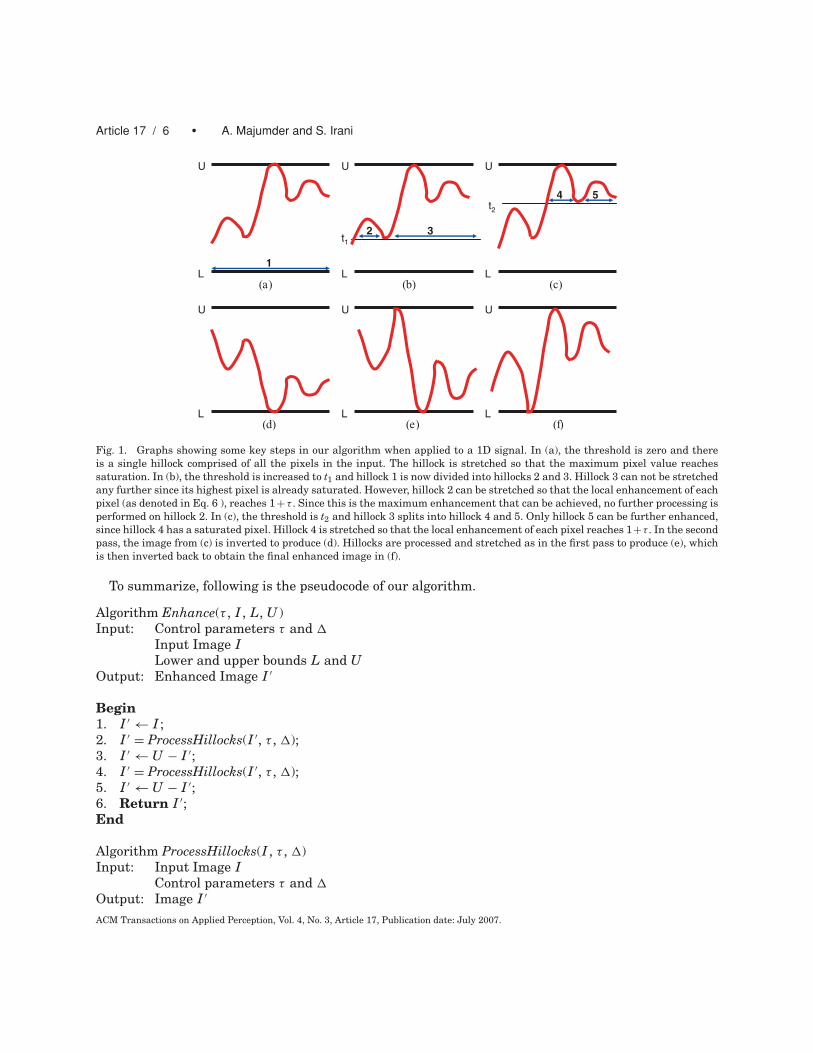
Fig. 1. Graphs showing some key steps in our algorithm when applied to a 1D signal. In (a), the threshold is zero and there

is a single hillock comprised of all the pixels in the input. The hillock is stretched so that the maximum pixel value reaches

saturation. In (b), the threshold is increased to t1 and hillock 1 is now divided into hillocks 2 and 3. Hillock 3 can not be stretched

any further since its highest pixel is already saturated. However, hillock 2 can be stretched so that the local enhancement of each

pixel (as denoted in Eq. 6 ), reaches 1 + τ . Since this is the maximum enhancement that can be achieved, no further processing is

performed on hillock 2. In (c), the threshold is t2 and hillock 3 splits into hillock 4 and 5. Only hillock 5 can be further enhanced,

since hillock 4 has a saturated pixel. Hillock 4 is stretched so that the local enhancement of each pixel reaches 1+τ . In the second

pass, the image from (c) is inverted to produce (d). Hillocks are processed and stretched as in the first pass to produce (e), which

is then inverted back to obtain the final enhanced image in (f).

To summarize, following is the pseudocode of our algorithm.

Algorithm Enhance(τ , I , L, U )Input: Control parameters τ and �

Input Image ILower and upper bounds L and U

Output: Enhanced Image I ′

Begin1. I ′ ← I ;2. I ′ = ProcessHillocks(I ′, τ , �);3. I ′ ← U − I ′;4. I ′ = ProcessHillocks(I ′, τ , �);5. I ′ ← U − I ′;6. Return I ′;End

Algorithm ProcessHillocks(I , τ , �)Input: Input Image I

Control parameters τ and �

Output: Image I ′



(a) (b) (c)

(d) (e) (f)

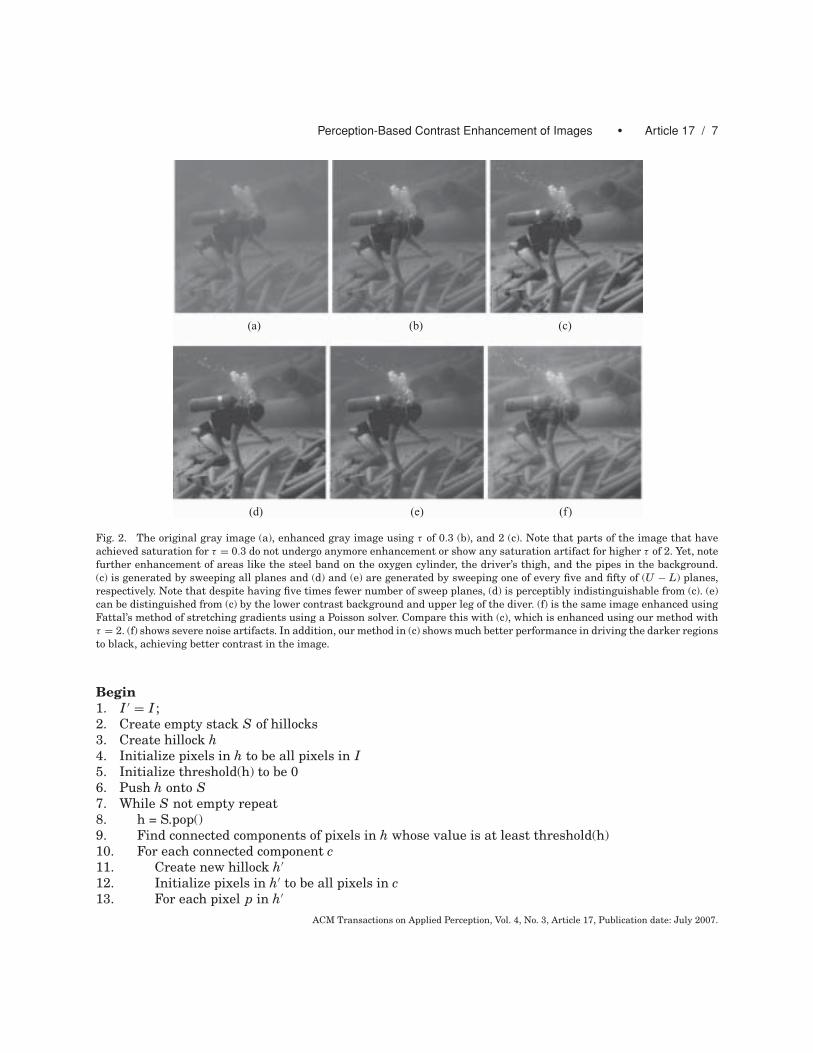
Fig. 2. The original gray image (a), enhanced gray image using τ of 0.3 (b), and 2 (c). Note that parts of the image that have

achieved saturation for τ = 0.3 do not undergo anymore enhancement or show any saturation artifact for higher τ of 2. Yet, note

further enhancement of areas like the steel band on the oxygen cylinder, the driver’s thigh, and the pipes in the background.

(c) is generated by sweeping all planes and (d) and (e) are generated by sweeping one of every five and fifty of (U − L) planes,

respectively. Note that despite having five times fewer number of sweep planes, (d) is perceptibly indistinguishable from (c). (e)

can be distinguished from (c) by the lower contrast background and upper leg of the diver. (f) is the same image enhanced using

Fattal’s method of stretching gradients using a Poisson solver. Compare this with (c), which is enhanced using our method with

τ = 2. (f) shows severe noise artifacts. In addition, our method in (c) shows much better performance in driving the darker regions

to black, achieving better contrast in the image.

Begin1. I ′ = I ;2. Create empty stack S of hillocks3. Create hillock h4. Initialize pixels in h to be all pixels in I5. Initialize threshold(h) to be 06. Push h onto S7. While S not empty repeat8. h = S.pop()9. Find connected components of pixels in h whose value is at least threshold(h)10. For each connected component c11. Create new hillock h′

12. Initialize pixels in h′ to be all pixels in c13. For each pixel p in h′



14. I ′(p) = (1 + s) ∗ (I ′(p) − t) + t15. where t is threshold(h) and s is the

maximum value over the entire hillock such that none of the constraints are violated.16. Let threshold(h′) be the minimum of I (p) over all pixels p

in h′ that are local minima or saddle points and I (p) isat least threshold (h′)

17. Push h′ onto S.End

Enhance calls the main routine ProcessHillocks on the original image and then on the inverted imageso that hillocks get pushed upward and valleys get pushed downward. ProcessHillocks maintains astack of hillocks. Each hillock maintains a set of pixels, which is disjoint from the pixels in any otherhillock. Each hillock also maintains a threshold parameter. In each iteration, the top hillock is poppedand the threshold is applied to all the pixels in the hillock. These pixels whose value is above thethreshold generate an underlying graph with edges between neighboring pixels. We then compute theconnected components of this graph and create a new hillock for each component. In Step 14, all thepixels in each component are then stretched upward as much as possible without violating any of thepredefined constraints. Threshold are moved upward and all the resulting hillocks are pushed onto thestack.

3.4 Results and Performance

Figure 2 shows the result of applying our method to low-contrast gray images for different values of τ .Note that even after our first optimization of sweeping planes at local minima, maxima and the saddlepoints, the number of sweep planes can be quite high, i.e., s can be of O(U − L). Hence, for a betterperformance, we studied the effect of skipping some of the sweep planes and found that we can increasethe performance by at least an order of magnitude before seeing visible differences. Figure 3 illustratesthis.

Figure 4 compares our method with standard techniques for contrast enhancement that uses globaland local histogram equalization, respectively. Figure 2 compares our method on gray images withthe recent method proposed in Fattal et al. [2002] that stretches the gradient image directly and thengenerates the enhanced image from the modified gradient field using a Poisson solver. Figure 5 showsthe result of our method on some medical images.

With the ideal parameter of � = 1, our optimized code takes about 10 s to process a 500 × 500 image.However, by setting � = 10, we can process the same image in about a couple of seconds. Figure 6 showsthe result of our contrast enhancement method on a high-resolution image of 1.5 megapixels with thesame �, which took around 6 s to process.

3.5 Evaluation

The advantage of our formulation of contrast enhancement as an optimization problem lies in thefact that the objective function, defined in Eq. (5), can be directly used as a metric to evaluate theamount of average contrast enhancement (ACE) achieved across the whole image. Note that accordingto the constraints of the optimization problem, the maximum average contrast that can be achievedwithout respecting saturation constraints is given by 1+τ . The saturation constraints restrict the actualenhancement achieved to less than or equal to 1 + τ , while keeping the image free of any artifacts.However, as τ increases, the effect of the saturation constraint becomes stronger, since larger numberof pixels reach saturation when being enhanced and, hence, needs to be restricted not to enhance to



(a) (b) (c)

(d) (e) (f)

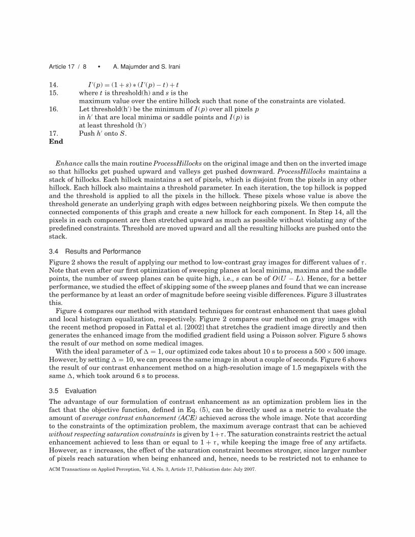
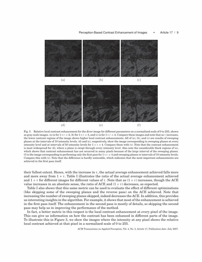
Fig. 3. Relative local contrast enhancement for the diver image for different parameters on a normalized scale of 0 to 255, shown

as gray scale images. (a) is for 1+τ = 2, (b) for 1+τ = 3, and (c) is for 1+τ = 4. Compare these images and note that as τ increases,

the lower contrast regions of the image shows higher local contrast enhancements. All of (a), (b), and (c) are results of sweeping

planes at the intervals of 10 intensity levels. (d) and (e), respectively, show the image corresponding to sweeping planes at every

intensity level and at intervals of 50 intensity levels for 1 + τ = 4. Compare these with (c). Note that the contrast enhancement

is most widespread for (d), where a plane is swept through every intensity level. Also note the considerable black regions of (e),

which shows that contrast enhancement has not occurred in many pixels because of the large interval of the sweeping planes.

(f) is the image corresponding to performing only the first pass for 1+τ = 4 and sweeping planes or intervals of 10 intensity levels.

Compare this with (c). Note that the difference is hardly noticeable, which indicates that the most important enhancements are

achieved in the first pass itself.

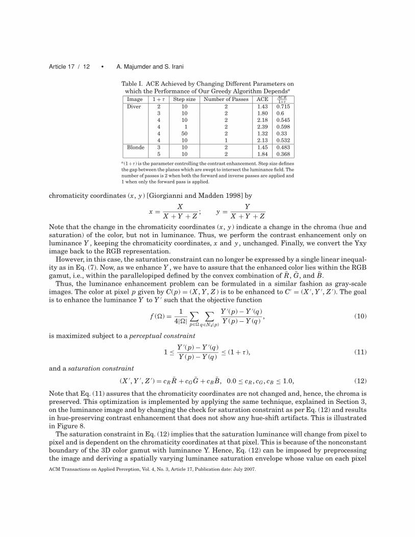
their fullest extent. Hence, with the increase in τ , the actual average enhancement achieved falls moreand more away from 1 + τ . Table I illustrates the ratio of the actual average enhancement achievedand 1 + τ for different images for different values of τ . Note that as (1 + τ ) increases, though the ACEvalue increases in an absolute sense, the ratio of ACE and (1 + τ ) decreases, as expected.

Table I also shows that this same metric can be used to evaluate the effect of different optimizations(like skipping some of the sweeping planes and the reverse pass) on the ACE achieved. Note thatincreasing the number of sweeping planes skipped, indeed decreases the ACE. In addition, this providesus interesting insights in the algorithm. For example, it shows that most of the enhancement is achievedin the first pass itself. The enhancement in the second pass is mostly of details, so skipping the secondpass may help us in improving the performance of the method.

In fact, a better metric in this respect is the local contrast enhancement at every pixel of the image.This can give us information on how the contrast has been enhanced in different parts of the image.To illustrate this in Figure 3, we show the images where the intensity at any pixel shows the relativelocal contrast achieved at that pixel in a normalized scale of 0 to 255.



(a) (b)

(c) (d)

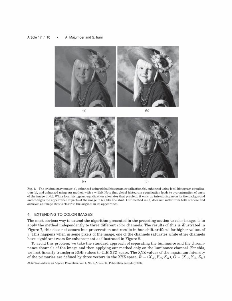
Fig. 4. The original gray image (a), enhanced using global histogram equalization (b), enhanced using local histogram equaliza-

tion (c), and enhanced using our method with τ = 1(d). Note that global histogram equalization leads to oversaturation of parts

of the image in (b). While local histogram equalization alleviates that problem, it ends up introducing noise in the background

and changes the appearance of parts of the image in (c), like the shirt. Our method in (d) does not suffer from both of these and

achieves an image that is closer to the original in its appearance.

4. EXTENDING TO COLOR IMAGES

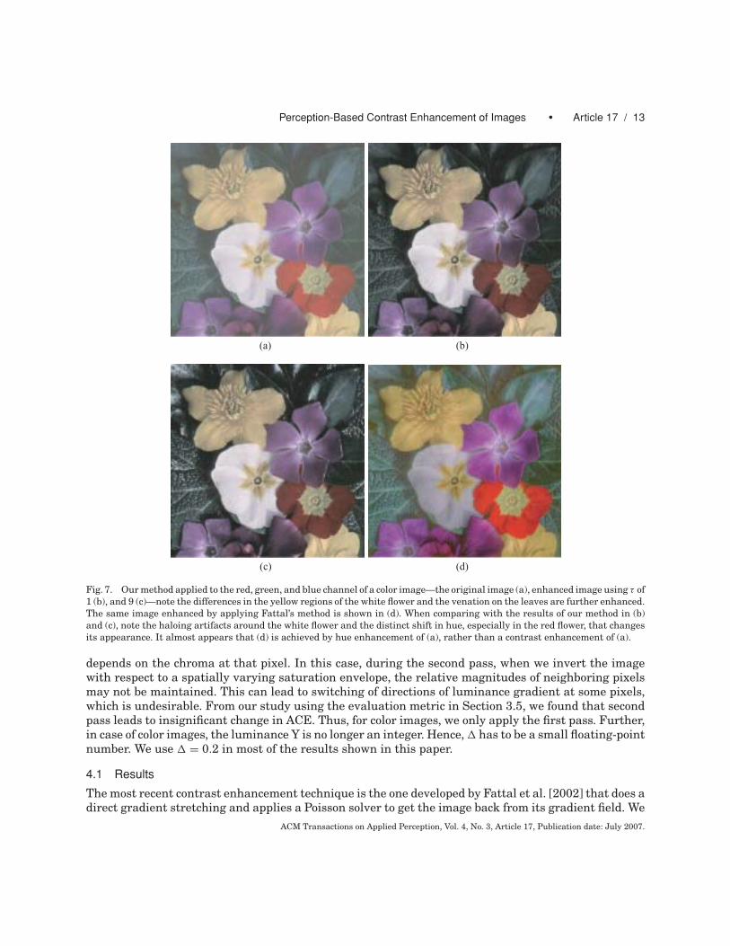
The most obvious way to extend the algorithm presented in the preceding section to color images is toapply the method independently to three different color channels. The results of this is illustrated inFigure 7, this does not assure hue preservation and results in hue-shift artifacts for higher values ofτ . This happens when in some pixels of the image, one of the channels saturates while other channelshave significant room for enhancement as illustrated in Figure 8.

To avoid this problem, we take the standard approach of separating the luminance and the chromi-nance channels of the image and then applying our method only on the luminance channel. For this,we first linearly transform RGB values to CIE XYZ space. The XYZ values of the maximum intensityof the primaries are defined by three vectors in the XYZ space, R = (X R , Y R , Z R), G = (X G , YG , Z G)



(a) (b)

(c) (d)

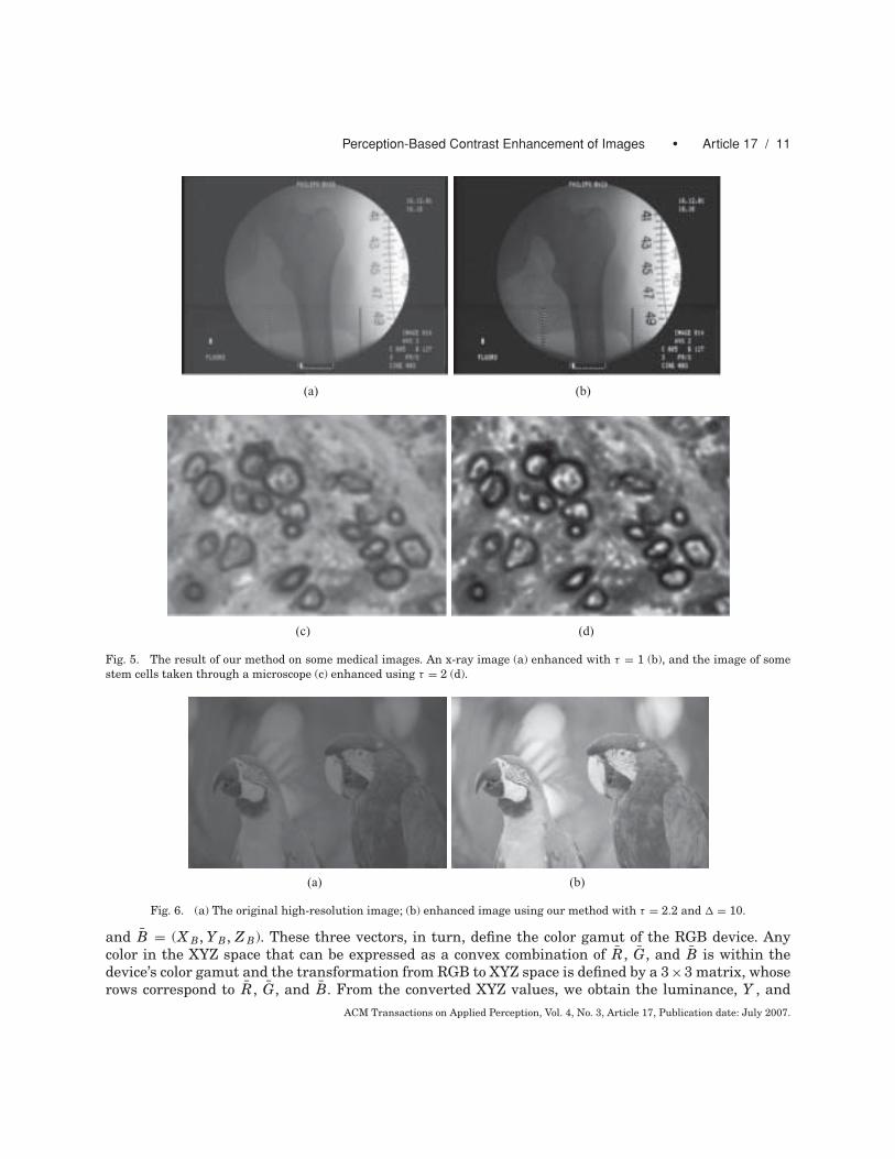
Fig. 5. The result of our method on some medical images. An x-ray image (a) enhanced with τ = 1 (b), and the image of some

stem cells taken through a microscope (c) enhanced using τ = 2 (d).

(a) (b)

Fig. 6. (a) The original high-resolution image; (b) enhanced image using our method with τ = 2.2 and � = 10.

and B = (X B, Y B, Z B). These three vectors, in turn, define the color gamut of the RGB device. Anycolor in the XYZ space that can be expressed as a convex combination of R, G, and B is within thedevice’s color gamut and the transformation from RGB to XYZ space is defined by a 3×3 matrix, whoserows correspond to R, G, and B. From the converted XYZ values, we obtain the luminance, Y , and



Table I. ACE Achieved by Changing Different Parameters on

which the Performance of Our Greedy Algorithm Dependsa

Image 1 + τ Step size Number of Passes ACE ACE1+τ

Diver 2 10 2 1.43 0.715

3 10 2 1.80 0.6

4 10 2 2.18 0.545

4 1 2 2.39 0.598

4 50 2 1.32 0.33

4 10 1 2.13 0.532

Blonde 3 10 2 1.45 0.483

5 10 2 1.84 0.368

a(1+τ ) is the parameter controlling the contrast enhancement. Step size defines

the gap between the planes which are swept to intersect the luminance field. The

number of passes is 2 when both the forward and inverse passes are applied and

1 when only the forward pass is applied.

chromaticity coordinates (x, y) [Giorgianni and Madden 1998] by

x = XX + Y + Z

; y = YX + Y + Z

Note that the change in the chromaticity coordinates (x, y) indicate a change in the chroma (hue andsaturation) of the color, but not in luminance. Thus, we perform the contrast enhancement only onluminance Y , keeping the chromaticity coordinates, x and y , unchanged. Finally, we convert the Yxyimage back to the RGB representation.

However, in this case, the saturation constraint can no longer be expressed by a single linear inequal-ity as in Eq. (7). Now, as we enhance Y , we have to assure that the enhanced color lies within the RGBgamut, i.e., within the parallelopiped defined by the convex combination of R, G, and B.

Thus, the luminance enhancement problem can be formulated in a similar fashion as gray-scaleimages. The color at pixel p given by C(p) = (X , Y , Z ) is to be enhanced to C′ = (X ′, Y ′, Z ′). The goalis to enhance the luminance Y to Y ′ such that the objective function

f (�) = 1

4|�|∑p∈�

∑q∈N4(p)

Y ′(p) − Y ′(q)

Y (p) − Y (q), (10)

is maximized subject to a perceptual constraint

1 ≤ Y ′(p) − Y ′(q)

Y (p) − Y (q)≤ (1 + τ ), (11)

and a saturation constraint

(X ′, Y ′, Z ′) = cR R + cGG + cB B, 0.0 ≤ cR , cG , cB ≤ 1.0, (12)

Note that Eq. (11) assures that the chromaticity coordinates are not changed and, hence, the chroma ispreserved. This optimization is implemented by applying the same technique, explained in Section 3,on the luminance image and by changing the check for saturation constraint as per Eq. (12) and resultsin hue-preserving contrast enhancement that does not show any hue-shift artifacts. This is illustratedin Figure 8.

The saturation constraint in Eq. (12) implies that the saturation luminance will change from pixel topixel and is dependent on the chromaticity coordinates at that pixel. This is because of the nonconstantboundary of the 3D color gamut with luminance Y. Hence, Eq. (12) can be imposed by preprocessingthe image and deriving a spatially varying luminance saturation envelope whose value on each pixel



(a) (b)

(c) (d)

Fig. 7. Our method applied to the red, green, and blue channel of a color image—the original image (a), enhanced image using τ of

1 (b), and 9 (c)—note the differences in the yellow regions of the white flower and the venation on the leaves are further enhanced.

The same image enhanced by applying Fattal’s method is shown in (d). When comparing with the results of our method in (b)

and (c), note the haloing artifacts around the white flower and the distinct shift in hue, especially in the red flower, that changes

its appearance. It almost appears that (d) is achieved by hue enhancement of (a), rather than a contrast enhancement of (a).

depends on the chroma at that pixel. In this case, during the second pass, when we invert the imagewith respect to a spatially varying saturation envelope, the relative magnitudes of neighboring pixelsmay not be maintained. This can lead to switching of directions of luminance gradient at some pixels,which is undesirable. From our study using the evaluation metric in Section 3.5, we found that secondpass leads to insignificant change in ACE. Thus, for color images, we only apply the first pass. Further,in case of color images, the luminance Y is no longer an integer. Hence, � has to be a small floating-pointnumber. We use � = 0.2 in most of the results shown in this paper.

4.1 Results

The most recent contrast enhancement technique is the one developed by Fattal et al. [2002] that does adirect gradient stretching and applies a Poisson solver to get the image back from its gradient field. We



(a) (b) (c)

(d) (e) (f)

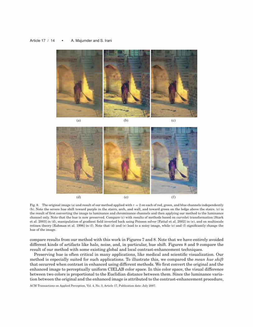
Fig. 8. The original image (a) and result of our method applied with τ = 2 on each of red, green, and blue channels independently

(b). Note the severe hue shift toward purple in the stairs, arch, and wall, and toward green on the ledge above the stairs. (c) is

the result of first converting the image to luminance and chrominance channels and then applying our method to the luminance

channel only. Note that the hue is now preserved. Compare (c) with results of methods based on curvelet transformation [Stark

et al. 2003] in (d), manipulation of gradient field inverted back using Poisson solver [Fattal et al. 2002] in (e), and on multiscale

retinex theory [Rahman et al. 1996] in (f). Note that (d) and (e) lead to a noisy image, while (e) and (f) significantly change the

hue of the image.

compare results from our method with this work in Figures 7 and 8. Note that we have entirely avoideddifferent kinds of artifacts like halo, noise, and, in particular, hue shift. Figures 8 and 9 compare theresult of our method with some existing global and local contrast-enhancement techniques.

Preserving hue is often critical in many applications, like medical and scientific visualization. Ourmethod is especially suited for such applications. To illustrate this, we compared the mean hue shiftthat occurred when contrast in enhanced using different methods. We first convert the original and theenhanced image to perceptually uniform CIELAB color space. In this color space, the visual differencebetween two colors is proportional to the Euclidian distance between them. Since the luminance varia-tion between the original and the enhanced image is attributed to the contrast-enhancement procedure,



(a) (b)

(c) (d)

(e) (f)

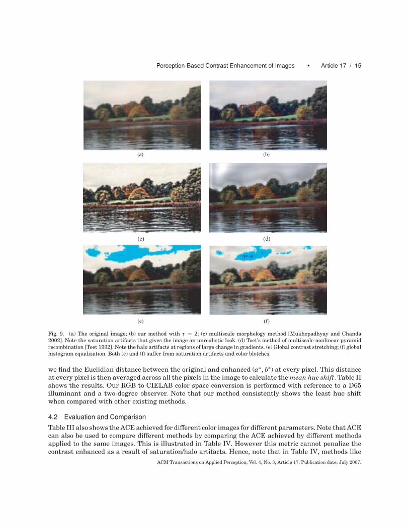
Fig. 9. (a) The original image; (b) our method with τ = 2; (c) multiscale morphology method [Mukhopadhyay and Chanda

2002]. Note the saturation artifacts that gives the image an unrealistic look. (d) Toet’s method of multiscale nonlinear pyramid

recombination [Toet 1992]. Note the halo artifacts at regions of large change in gradients. (e) Global contrast stretching; (f) global

histogram equalization. Both (e) and (f) suffer from saturation artifacts and color blotches.

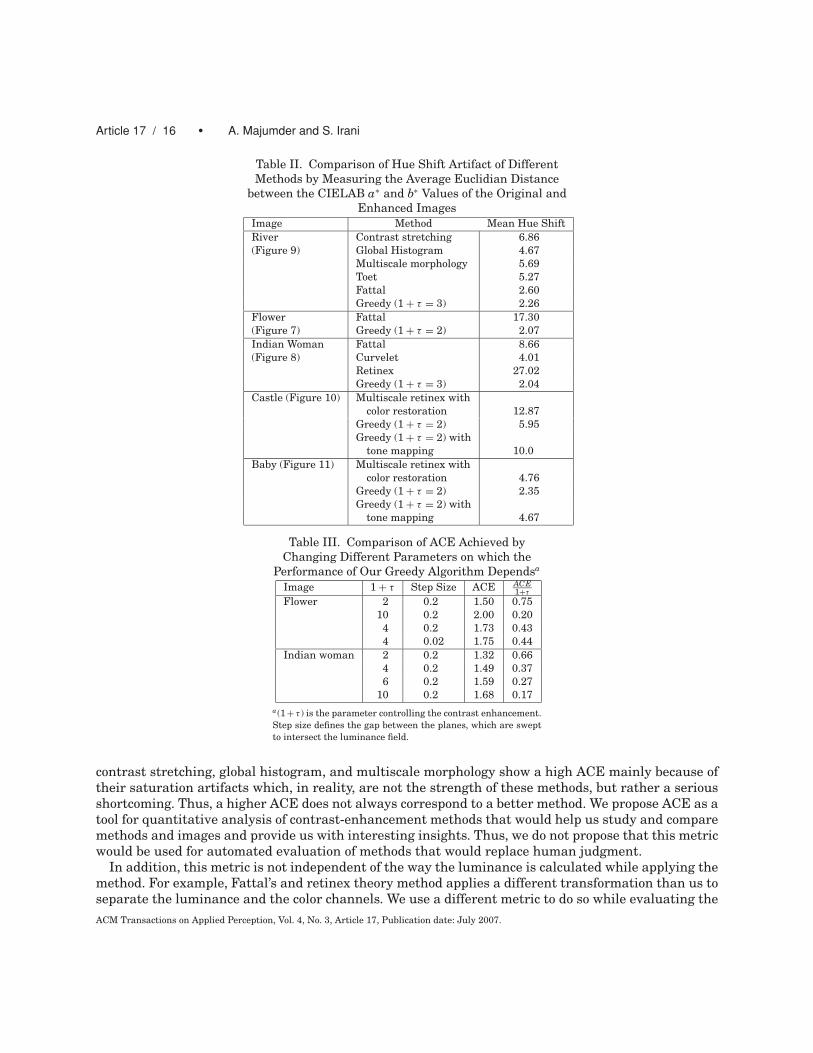
we find the Euclidian distance between the original and enhanced (a∗, b∗) at every pixel. This distanceat every pixel is then averaged across all the pixels in the image to calculate the mean hue shift. Table IIshows the results. Our RGB to CIELAB color space conversion is performed with reference to a D65illuminant and a two-degree observer. Note that our method consistently shows the least hue shiftwhen compared with other existing methods.

4.2 Evaluation and Comparison

Table III also shows the ACE achieved for different color images for different parameters. Note that ACEcan also be used to compare different methods by comparing the ACE achieved by different methodsapplied to the same images. This is illustrated in Table IV. However this metric cannot penalize thecontrast enhanced as a result of saturation/halo artifacts. Hence, note that in Table IV, methods like



Table II. Comparison of Hue Shift Artifact of Different

Methods by Measuring the Average Euclidian Distance

between the CIELAB a∗ and b∗ Values of the Original and

Enhanced Images

Image Method Mean Hue Shift

River Contrast stretching 6.86

(Figure 9) Global Histogram 4.67

Multiscale morphology 5.69

Toet 5.27

Fattal 2.60

Greedy (1 + τ = 3) 2.26

Flower Fattal 17.30

(Figure 7) Greedy (1 + τ = 2) 2.07

Indian Woman Fattal 8.66

(Figure 8) Curvelet 4.01

Retinex 27.02

Greedy (1 + τ = 3) 2.04

Castle (Figure 10) Multiscale retinex with

color restoration 12.87

Greedy (1 + τ = 2) 5.95

Greedy (1 + τ = 2) with

tone mapping 10.0

Baby (Figure 11) Multiscale retinex with

color restoration 4.76

Greedy (1 + τ = 2) 2.35

Greedy (1 + τ = 2) with

tone mapping 4.67

Table III. Comparison of ACE Achieved by

Changing Different Parameters on which the

Performance of Our Greedy Algorithm Dependsa

Image 1 + τ Step Size ACE ACE1+τ

Flower 2 0.2 1.50 0.75

10 0.2 2.00 0.20

4 0.2 1.73 0.43

4 0.02 1.75 0.44

Indian woman 2 0.2 1.32 0.66

4 0.2 1.49 0.37

6 0.2 1.59 0.27

10 0.2 1.68 0.17

a(1 + τ ) is the parameter controlling the contrast enhancement.

Step size defines the gap between the planes, which are swept

to intersect the luminance field.

contrast stretching, global histogram, and multiscale morphology show a high ACE mainly because oftheir saturation artifacts which, in reality, are not the strength of these methods, but rather a seriousshortcoming. Thus, a higher ACE does not always correspond to a better method. We propose ACE as atool for quantitative analysis of contrast-enhancement methods that would help us study and comparemethods and images and provide us with interesting insights. Thus, we do not propose that this metricwould be used for automated evaluation of methods that would replace human judgment.

In addition, this metric is not independent of the way the luminance is calculated while applying themethod. For example, Fattal’s and retinex theory method applies a different transformation than us toseparate the luminance and the color channels. We use a different metric to do so while evaluating the



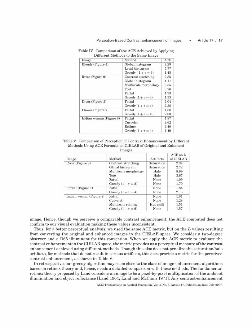
Table IV. Comparison of the ACE Achieved by Applying

Different Methods to the Same Image

Image Method ACE

Blonde (Figure 4) Global histogram 2.29

Local histogram 5.77

Greedy ( 1 + τ = 3) 1.45

River (Figure 9) Contrast stretching 2.85

Global histogram 4.11

Multiscale morphology 9.55

Toet 3.76

Fattal 1.93

Greedy (1 + τ = 3) 1.33

Diver (Figure 2) Fattal 2.04

Greedy (1 + τ = 4) 2.38

Flower (Figure 7) Fattal 1.68

Greedy (1 + τ = 10) 2.00

Indian woman (Figure 8) Fattal 1.87

Curvelet 2.62

Retinex 2.40

Greedy (1 + τ = 4) 1.49

Table V. Comparison of Perception of Contrast Enhancement by Different

Methods Using ACE Formula on CIELAB of Original and Enhanced

Images

ACE on L

Image Method Artifacts of CIELAB

River (Figure 9) Contrast stretching Saturation 2.34

Global histogram Saturation 2.72

Multiscale morphology Halo 8.99

Tote Halo 3.67

Fattal None 1.09

Greedy (1 + τ = 2) None 1.70

Flower (Figure 7) Fattal None 1.84

Greedy (1 + τ = 4) None 2.15

Indian woman (Figure 8) Fattal None 1.01

Curvelet None 1.28

Multiscale retinex Hue shift 1.51

Greedy (1 + τ = 6) None 1.57

image. Hence, though we perceive a comparable contrast enhancement, the ACE computed does notconfirm to our visual evaluation making these values inconsistent.

Thus, for a better perceptual analysis, we used the same ACE metric, but on the L values resultingfrom converting the original and enhanced images in the CIELAB space. We consider a two-degreeobserver and a D65 illuminant for this conversion. When we apply the ACE metric to evaluate thecontrast enhancement in the CIELAB space, the metric provides us a perceptual measure of the contrastenhancement achieved using different methods. Though this also does not penalize the saturation/haloartifacts, for methods that do not result in serious artifacts, this does provide a metric for the perceivedcontrast enhancement, as shown in Table V.

In retrospective, our greedy algorithm may seem close to the class of image-enhancement algorithmsbased on retinex theory and, hence, needs a detailed comparison with these methods. The fundamentalretinex theory proposed by Land considers an image to be a pixel-by-pixel multiplication of the ambientillumination and object reflectance [Land 1964; Land and McCann 1971]. Any contrast-enhancement



(a) (b)

(c) (d)

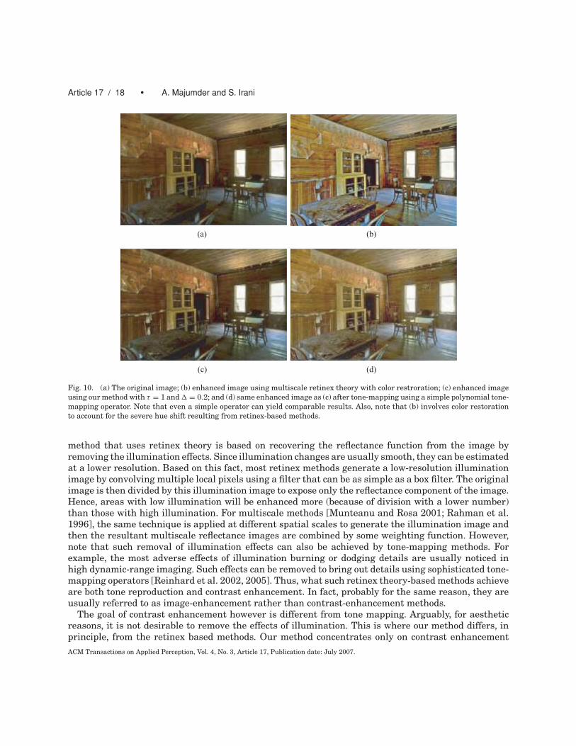
Fig. 10. (a) The original image; (b) enhanced image using multiscale retinex theory with color restroration; (c) enhanced image

using our method with τ = 1 and � = 0.2; and (d) same enhanced image as (c) after tone-mapping using a simple polynomial tone-

mapping operator. Note that even a simple operator can yield comparable results. Also, note that (b) involves color restoration

to account for the severe hue shift resulting from retinex-based methods.

method that uses retinex theory is based on recovering the reflectance function from the image byremoving the illumination effects. Since illumination changes are usually smooth, they can be estimatedat a lower resolution. Based on this fact, most retinex methods generate a low-resolution illuminationimage by convolving multiple local pixels using a filter that can be as simple as a box filter. The originalimage is then divided by this illumination image to expose only the reflectance component of the image.Hence, areas with low illumination will be enhanced more (because of division with a lower number)than those with high illumination. For multiscale methods [Munteanu and Rosa 2001; Rahman et al.1996], the same technique is applied at different spatial scales to generate the illumination image andthen the resultant multiscale reflectance images are combined by some weighting function. However,note that such removal of illumination effects can also be achieved by tone-mapping methods. Forexample, the most adverse effects of illumination burning or dodging details are usually noticed inhigh dynamic-range imaging. Such effects can be removed to bring out details using sophisticated tone-mapping operators [Reinhard et al. 2002, 2005]. Thus, what such retinex theory-based methods achieveare both tone reproduction and contrast enhancement. In fact, probably for the same reason, they areusually referred to as image-enhancement rather than contrast-enhancement methods.

The goal of contrast enhancement however is different from tone mapping. Arguably, for aestheticreasons, it is not desirable to remove the effects of illumination. This is where our method differs, inprinciple, from the retinex based methods. Our method concentrates only on contrast enhancement



(a) (b)

(c) (d)

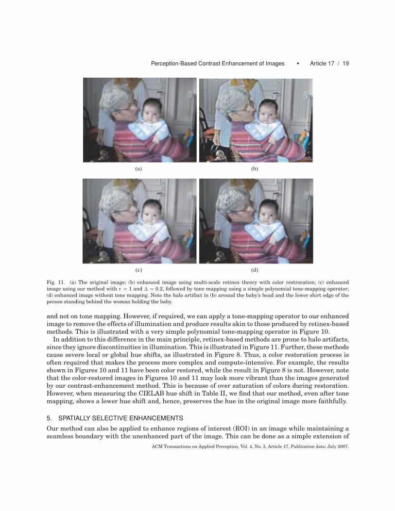
Fig. 11. (a) The original image; (b) enhanced image using multi-scale retinex theory with color restroration; (c) enhanced

image using our method with τ = 1 and � = 0.2, followed by tone mapping using a simple polynomial tone-mapping operator;

(d) enhanced image without tone mapping. Note the halo artifact in (b) around the baby’s head and the lower shirt edge of the

person standing behind the woman holding the baby.

and not on tone mapping. However, if required, we can apply a tone-mapping operator to our enhancedimage to remove the effects of illumination and produce results akin to those produced by retinex-basedmethods. This is illustrated with a very simple polynomial tone-mapping operator in Figure 10.

In addition to this difference in the main principle, retinex-based methods are prone to halo artifacts,since they ignore discontinuities in illumination. This is illustrated in Figure 11. Further, these methodscause severe local or global hue shifts, as illustrated in Figure 8. Thus, a color restoration process isoften required that makes the process more complex and compute-intensive. For example, the resultsshown in Figures 10 and 11 have been color restored, while the result in Figure 8 is not. However, notethat the color-restored images in Figures 10 and 11 may look more vibrant than the images generatedby our contrast-enhancement method. This is because of over saturation of colors during restoration.However, when measuring the CIELAB hue shift in Table II, we find that our method, even after tonemapping, shows a lower hue shift and, hence, preserves the hue in the original image more faithfully.

5. SPATIALLY SELECTIVE ENHANCEMENTS

Our method can also be applied to enhance regions of interest (ROI) in an image while maintaining aseamless boundary with the unenhanced part of the image. This can be done as a simple extension of



(a) (b)

(c) (d)

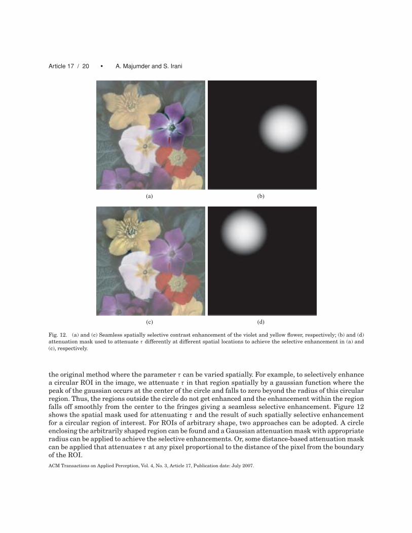
Fig. 12. (a) and (c) Seamless spatially selective contrast enhancement of the violet and yellow flower, respectively; (b) and (d)

attenuation mask used to attenuate τ differently at different spatial locations to achieve the selective enhancement in (a) and

(c), respectively.

the original method where the parameter τ can be varied spatially. For example, to selectively enhancea circular ROI in the image, we attenuate τ in that region spatially by a gaussian function where thepeak of the gaussian occurs at the center of the circle and falls to zero beyond the radius of this circularregion. Thus, the regions outside the circle do not get enhanced and the enhancement within the regionfalls off smoothly from the center to the fringes giving a seamless selective enhancement. Figure 12shows the spatial mask used for attenuating τ and the result of such spatially selective enhancementfor a circular region of interest. For ROIs of arbitrary shape, two approaches can be adopted. A circleenclosing the arbitrarily shaped region can be found and a Gaussian attenuation mask with appropriateradius can be applied to achieve the selective enhancements. Or, some distance-based attenuation maskcan be applied that attenuates τ at any pixel proportional to the distance of the pixel from the boundaryof the ROI.



6. CONCLUSION

In conclusion, we use that fact that the suprathreshold human contrast sensitivity follows the WeberLaw to achieve contrast enhancements of images. We apply a greedy algorithm to the image in its nativeresolution without requiring any expensive image segmentation operation. We pose the contrast en-hancement as an optimization problem that maximizes an objective function defining the local averagecontrast enhancement (ACE) in an image subject to constraints that control the contrast enhancementby a single parameter τ . We extend this method to color images where hue is preserved while enhancingonly the luminance contrast. In addition, we vary the parameter τ spatially over the image to achievespatially selective enhancement. Finally, we show that the ACE defined by the objective function canact as a metric to compare the contrast enhancement achieved for different methods and differentparameters thereof.

Future work in this direction will include exploring the possibility of extending this to video by addingthe additional temporal dimension. We also intend to pursue applications dealing with 1D signals, suchas sound. Since our method treats the image as a height field, it could have interesting applicationsin terrain or mesh editing. Finally, exploring the possibility of implementing this method on graphicprocessing units would allow this method to be used interactively.

ACKNOWLEDGMENTS

We acknowledge Prof. Raanan Fattal of University of California, Berkeley who provided us some imagesfor comparing and validating our results. We acknowledge NSF (Grant CCF-0514082) for partiallysupporting the second author of the paper.

REFERENCES

BARTEN, P. G. 1999. Contrast sensitivity of the human eye and its effects on image quality. SPIE - The International Societyfor Optical Engineering, P.O. Box 10 Bellingham Washington 98227-0010. ISBN 0-8194-3496-5.

BOCCIGNONE, G. AND PICARIELLO, A. 1997. Multiscale contrast enhancement of medical images. In Proceedings of ICASSP.

BURT, P. J. AND ADELSON, E. H. 1983. A multiresolution spline with application to image mosaics. ACM Transactions onGraphics 2, 4, 217–236.

DEBEVEC, P. E. AND MALIK, J. 1997. Recovering high dynamic range radiance maps from photographs. In Proceedings of ACMSIGGRAPH, 369–378.

FATTAL, R., LISCHINSKI, D., AND WERMAN, M. 2002. Gradient domain high dynamic range compression. ACM Transactions onGraphics, Proceedings of ACM Siggraph 21, 3, 249–256.

GEORGESON, M. AND SULLIVAN, G. 1975. Contrast constancy: Deblurring in human vision by spatial frequency channels. Journalof Physiology 252, 627–656.

GIORGIANNI, E. J. AND MADDEN, T. E. 1998. Digital Color Management: Encoding Solutions. Addison Wesley, Reading, MA.

HANMANDLU, M., JHA, D., AND SHARMA, R. 2000. Color image enhancement by fuzzy intensification. In Proceedings of Interna-tional Conference on Pattern Recognition.

HANMANDLU, M., JHA, D., AND SHARMA, R. 2001. Localized contrast enhancement of color images using clustering. In Proceedingsof IEEE International Conference on Information Technology: Coding and Computing (ITCC).

KINGDOM, F. A. A. AND WHITTLE, P. 1996. Contrast discrimination at high contrasts reveal the influence of local light adaptation

on contrast processing. Vision Research 36, 6, 817–829.

KOENDERINK, J. J. 1984. The structure of images. Biological Cybernetics 50, 5, 363–370.

LAND, E. 1964. The retinex. American Scientist 52, 2, 247–264.

LAND, E. AND MCCANN, J. 1971. Lightness and retinex theory. Journal of Optical Society of America 61, 1, 1–11.

MANTIUK, R., MYSZKOWSKI, K., AND SEIDEL, H.-P. S. 2006. A perceptual framework for contrast processing of high dynamic range

images. ACM Transactions on Applied Perception 3, 3.

MUKHOPADHYAY, S. AND CHANDA, B. 2002. Hue preserving color image enhancement using multi-scale morphology. IndianConference on Computer Vision, Graphics and Image Processing.



MUNTEANU, C. AND ROSA, A. 2001. Color image enhancement using evolutionary principles and the retinex theory of color

constancy. In Proceedings 2001 IEEE Signal Processing Society Workshop on Neural Networks for Signal Processing XI,

393–402.

OAKLEY, J. P. AND SATHERLEY, B. L. 1998. Improving image quality in poor visibility conditions using a physical model for

contrast degradation. IEEE Transactions on Image Processing 7, 167–179.

PELI, E. 1990. Contrast in complex images. Journal of Optical Society of America A 7, 10, 2032–2040.

PREZ, P., GANGNET, M., AND BLAKE, A. 2003. Poisson image editing. ACM Transactions on Graphics, Proceedings of ACMSiggraph 22, 3, 313–318.

RAHMAN, Z., JOBSON, D. J., , AND WOODELL, G. A. 1996. Multi-scale retinex for color image enhancement. IEEE InternationalConference on Image Processing.

REINHARD, E., STARK, M., SHIRLEY, P., AND FERWERDA, J. 2002. Photographic tone reproduction for digital images. ACM Trans-actions on Graphics (SIGGRAPH) 21, 3, 267–276.

REINHARD, E., WARD, G., PATTANAIK, S., AND DEBEVEC, P. 2005. High Dynamic Range Imaging. Morgan Kaufmann Pub. San

Francisco, CA.

SHYU, M. AND LEOU, J. 1998. A geneticle algorithm approach to color image enhancement. Pattern Recognition 31, 7, 871–880.

STARK, J.-L., MURTAGH, F., CANDES, E. J., AND DONOHO, D. L. 2003. Gray and color image contrast enhancement by curvelet

transform. IEEE Transactions on Image Processing 12, 6.

TOET, A. 1990. A hierarchical morphological image decomposition. Pattern Recognition Letters 11, 4, 267–274.

TOET, A. 1992. Multi-scale color image enhancement. Pattern Recognition Letters 13, 3, 167–174.

VALOIS, R. L. D. AND VALOIS, K. K. D. 1990. Spatial Vision. Oxford University Press, Oxford

VELDE, K. V. 1999. Multi-scale color image enhancement. In Proceedings on International Conference on Image Processing 3,

584–587.

WHITTLE, P. 1986. Increments and decrements: Luminance discrimination. Vision Research 26, 10, 1677–1691.

WILSON, H. 1991. Psychophysical models of spatial vision and hyperacuity. Vision and Visual Dysfunction: Spatial Vision, D.

Regan, Editor, Pan Macmillan, 64–86.

WITKIN, A. P. 1983. Scale-space filtering. In Proceedings of the 7th International Joint Conference on Artificial Intelligence,

1019–1022.

Received October 2006; revised May 2007; accepted June 2007


Documents

Perception-Based Contrast Enhancement of Imagesmajumder/docs/TAP07.pdf · Perception-Based Contrast Enhancement of Images • Article 17 / 3 the local contrast C are related by ∂C