PEER Performance-Based Earthquake Engineering Methodology:

Structural and Architectural Aspects

Van Nuys Testbed Committee

Pacific Earthquake Engineering Research Center

University of California, Berkeley

November 5, 2002

Author InstructionsEditing instructions

1. Leave “track changes” on.

2. Paste your text in your section. Follow the PEER Style Guide.

3. Rename the file “[your last name] Van Nuys Report [Day Month Year].doc”, and email it

to me (Porter) at keithp@caltech.edu, with cc to Helmut (krawinkler@stanford.edu).

4. If you change your text after sending it to me, accept all your previous edits in Track

Changes, and repeat the process.

Schedule

Section Responsible Due Inserted

1. Introduction1.1 Background Porter 4/15/02 5/1/021.2 Objectives Porter 4/15/02 5/1/021.3 Scope Porter 4/15/02 5/1/02

2. Components to be Tested2.1 Methodology Krawinkler 11/30/03

3. Hazard Analysis3.1 Conventional free-field hazard analysis Somerville 4/15/02 4/15/023.2 Variability in the Ground Motion… Somerville 4/15/02 4/15/023.3 Free-field hazard … improved IMs Cornell HK?3.4 Effects of Site Soil Profile… Kramer 10/1/03

4. Prediction of EDPs4.1 Analytical Modeling of Foundation Hutchinson 5/14/024.2 Analytical Modeling of Foundation-Structure System

Lowes 10/15/03

4.3 Validation of Analytical Models Lowes 10/15/034.4 Prediction of EDPs Miranda 9/15/034.5 Prediction of Collapse Probability Krawinkler ND. 4.6 Estimation of Casualties Miranda 10/15/03

4.6.1 Theoretical Means Cornell 8/31/034.6.2 Empirical Approach Shoaf 8/31/034.6.3 Application to Testbed Miranda 10/15/03

5. Prediction of Loss5.1 DM/EDP and DV/DM Relationships… Miranda, Lowes 8/15/02 3/15/025.2 Application of Loss and Downtime… Miranda 8/01/03

6. Propagation of Uncertainties Cornell 10/1/027. Relation to Current Engineering Approaches Heintz

7.1 Current Practice Heintz 5/02-7/027.2 Assessment of PEER Methodology Heintz 10/02-12/02

8. Societal Issues and Impact [Eliminated]

2

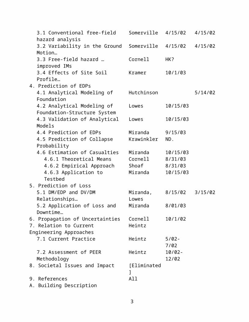
9. References AllA. Building Description

A.1 Summary Description Porter 4/15/02 3/18/02A.2 Structural Properties Porter 4/15/02 3/18/02A.3 Past Earthquake Damage Porter 4/15/02 3/18/02A.4 Occupancy Shoaf 8/31/03A.5 References Porter 4/15/02 3/18/02

3

Contents1 Introduction..................................................................................................................9

1.1 Background..........................................................................................................91.2 Objectives..........................................................................................................101.3 Scope..................................................................................................................11

2 Methodology Components to be Tested....................................................................142.1 Case Specific Summary of Methodology..........................................................14

3 Hazard Analysis.........................................................................................................153.1 Conventional Free-Field Hazard Analysis and Ground Motion Selection........15

3.1.1 Seismic Hazard..............................................................................................153.1.2 Uniform Hazard Spectra................................................................................153.1.3 Deaggregation of the Hazard.........................................................................173.1.4 Record Selection............................................................................................17

3.2 Variability in the Ground Motion Recordings...................................................203.2.1 Epistemic Uncertainty in Probabilistic Seismic Hazard Analysis.................25

3.3 Free-Field Hazard Analysis and Record Selection Based on Improved IMs....273.3.1 Brief General Discussion of IM’s and their issues........................................273.3.2 Process Used by IM Study Group to Evaluate and Select Improved IMs.....273.3.3 Candidate IMs for VN testbed. Brief justification for each...........................273.3.4 Results of IM studies for the VN testbed.......................................................273.3.5 Hazard Analysis of improved IM(’s).............................................................27

3.4 Effects of Site Soil Profile on IMs and Ground Motions..................................284 Prediction of EDPs....................................................................................................31

4.1 Analytical Modeling of Foundation...................................................................314.2 Analytical Modeling of Foundation-Structure System......................................34

4.2.1 Modeling Objectives......................................................................................344.2.2 Types of Models Employed...........................................................................354.2.3 Model Verification.........................................................................................354.2.4 Results............................................................................................................35

4.3 Validation of Analytical Models.......................................................................374.3.1 Experimental Data Used in Model Development and Validation.................374.3.2 Validation Protocol........................................................................................374.3.3 The EDP to DM Relationship........................................................................374.3.4 Structural Performance Data Base.................................................................37

4.4 Prediction of EDPs for Damage Assessment.....................................................394.4.1 General discussion of the role of EDP’s in the methodology........................394.4.2 Selection of EDP Vector................................................................................394.4.3 Results of EDP versus IM..............................................................................424.4.4 EDP Hazard Curves.......................................................................................424.4.5 Epistemic Uncertainty...................................................................................42

4

4.4.6 Prediction by Means of Simplified Approaches............................................424.5 Prediction of Probability of Collapse and of Casualties....................................42

4.5.1 Discussion of Collapse Estimation and its Role in Method..........................434.5.2 Models for Global and Local Collapse..........................................................434.5.3 Results of Collapse Predictions.....................................................................434.5.4 Estimation of Casualties................................................................................434.5.5 Epistemic Uncertainties.................................................................................434.5.6 Prediction by Means of Simplified Approaches............................................43

5 Prediction of Losses...................................................................................................445.1 DM/EDP and DV/DM Relationships................................................................44

5.1.1 Structural Elements........................................................................................445.1.2 Nonstructural Elements.................................................................................45

5.2 Application of Loss Estimation Methodology...................................................476 Propagation of Uncertainties from IM to DV............................................................507 Relation to Presently Accepted Engineering Approaches.........................................51

7.1 Current Practice of Engineering Evaluation......................................................517.1.1 Methodologies and Tools Currently in Use...................................................517.1.2 Communicating Performance to an Owner...................................................517.1.3 FEMA 356 Engineering Assessment of Van Nuys Testbed..........................51

7.2 A FEMA 356 retrofit design..............................................................................517.3 Engineering Assessment of the PEER PBEE Methodology..............................52

7.3.1 Comparison of FEMA 356 and PEER Methodologies..................................527.3.2 Implementation of the PEER Methodology in Engineering Practice............52

8 Societal Issues and Impact.........................................................................................538.1 Assessment of the PBEE Process......................................................................538.2 Commentary on Societal Implications...............................................................53

9 References..................................................................................................................5510 Glossary.................................................................................................................56

Appendix A. Pre-Northridge Building ConditionA.1 Summary DescriptionA.2 Structural PropertiesA.3 Past Earthquake DamageA.4 References

Appendix B. Retrofit DesignAppendix C. Design by PEER Methodology

5

Index of FiguresFig. 1. Overview of PEER analysis methodology........................................................................13Fig. 2. Variability in the ground motions of each set of ten scaled recordings for the longitudinal

and transverse components for each of three ground-motion levels.....................................22Fig. 3. Variability in the ground motions of each set of ten scaled recordings for the vertical

component for each of three ground motion levels...............................................................23Fig. 4. Comparison of the longitudinal and transverse response spectra averaged over the ten

scaled recordings for the 50% in 50 year ground motion level.............................................24Fig. 5. Comparison of the longitudinal and transverse response spectra averaged over the ten

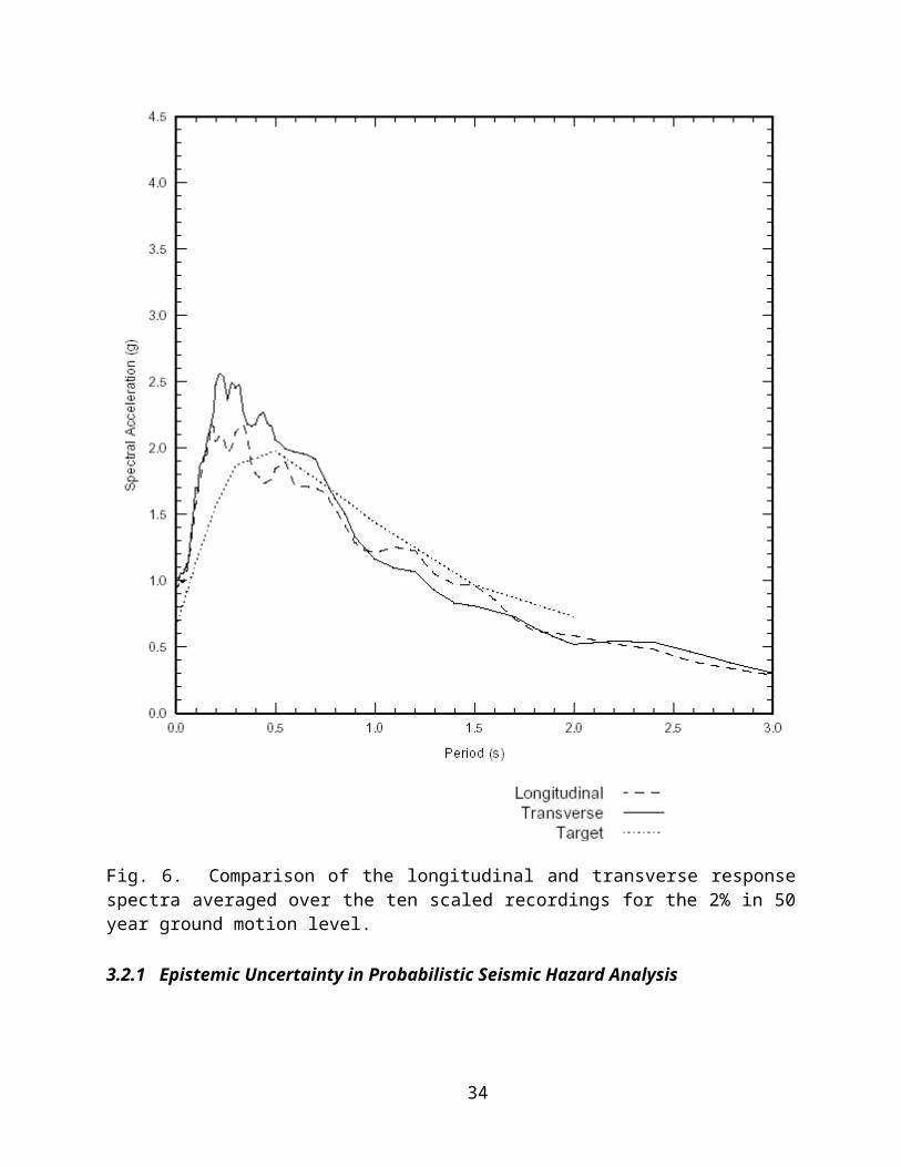
scaled recordings for the 10% in 50 year ground motion level.............................................25Fig. 6. Comparison of the longitudinal and transverse response spectra averaged over the ten

scaled recordings for the 2% in 50 year ground motion level...............................................26Fig. 7. Foundation plan and primary types of pile-pile-cap combinations.............................33Fig. 8. Interior and exterior pile-cap details..............................................................................34Fig. 9. Boring logs (reproduced from GeoSystems 1994).........................................................34Fig. 10. Location of the demonstration building: the “+” symbol above the “405” shield..........59Fig. 11. First floor architectural plan (Rissman and Rissman Associates, 1965).........................61Fig. 12. Second floor architectural plan (Rissman and Rissman Associates, 1965)....................62Fig. 13. Typical hotel suite floor plan (Rissman and Rissman Associates, 1965).......................63Fig. 14. Foundation and column plan. The plan is regular, with three bays in the transverse

direction, eight in the longitudinal direction. “C1” through “C36” refers to column numbers (designer’s notation)..............................................................................................................64

Fig. 15. South frame elevation, omitting stair tower at west end.................................................65Fig. 16. Floor beam and floor spandrel beam plans.....................................................................67Fig. 17. Arrangement of column steel (Rissman and Rissman Associates, 1965).......................68Fig. 18. Testbed building (star) relative to 1971 and 1994 earthquakes (EERI, 1994)................72Fig. 19. Instrument locations in 1971 San Fernando earthquake..................................................73Fig. 20. Spectral acceleration, 1971 ground-floor motions, longit. (left) and transverse (right)..73Fig. 21. Instrument locations after 1980.......................................................................................75Fig. 22. Spectral acceleration of ground-floor motions, 1994 longit. (left) and transverse (right).

...............................................................................................................................................77Fig. 23. Structural damage in 1994 Northridge earthquake, south frame (Trifunac et al., 1999) 79Fig. 24. Structural damage in 1994 Northridge earthquake, north frame (Trifunac et al., 1999) 80Fig. 25. Shearwalls added to south (left) and north frames (right) after the 1994 Northridge

earthquake. (Left: lines A-3, 7 and 8 from near to far. Right: lines D-8, 7, 5, and 3)...........80

6

Index of TablesTable 1. Equal-Hazard Response Spectra for the Van Nuys Building.........................................17Table 2. Deaggregation of uniform hazard spectra, 5% damping, soil, east (transverse) Sa at 1

second, at the Van Nuys building..........................................................................................18Table 3. Time histories representing 50% in 50 years hazard level at the Van Nuys Building. . .19Table 4. Time histories representing 10% in 50 years hazard level at the Van Nuys Building. . .20Table 5. Time histories representing 2% in 50 years hazard level at the Van Nuys building......20Table 6. Preliminary recommendations for elastic vertical, horizontal and rotational spring

stiffnesses..............................................................................................................................35Table 7. Column reinforcement schedule.....................................................................................69Table 8. Spandrel beam reinforcement schedule, floors 3 through 7...........................................70Table 9. Roof and second-floor spandrel beam reinforcement schedule......................................71Table 10. Approximate fundamental building periods (Islam, 1996)..........................................74Table 11. Events causing strong motion (Trifunac et al., 1999; CSMIP, 1994)..........................76Table 12. Recorded peak displacements and story drift ratios.....................................................78

7

1 IntroductionK.A Porter

1.1 BACKGROUND

Three structural design paradigms. Structural design comprises the selection of

structural, nonstructural, and geotechnical systems, and their materials and configuration, with

the goal of constructing a building, bridge, or other structure that will be safe and economical

under foreseeable circumstances. Historically, structural engineers have used allowable-stress

design (ASD) and load-and-resistance-factor design (LRFD), which focus on individual

structural elements and connections, and seek to ensure that none will experience loads or

deformation greater than it is capable of withstanding. An emerging approach, called

performance-based design (PBD), seeks to ensure that a designed facility as a whole will

perform in some predictable way, in terms of safety and functionality. Seismic aspects of PBD

are referred to as performance-based earthquake engineering (PBEE). PBEE therefore considers

the seismic reliability of the elements and connections, but also directly addresses the facility's

earthquake performance from the viewpoint of facility users, owners, and other stakeholders.

SEAOC, FEMA, and ASCE PBEE efforts. The PEER Center is not alone in developing

PBEE. The Structural Engineers Association of California (SEAOC) created an early sketch of

the objectives and methodologies of PBEE, in its Vision 2000 document (Office of Emergency

Services, 1995) and Conceptual Framework for Performance-Based Seismic Design (Structural

Engineers Association of California, 1999). SEAOC’s approach addresses performance in terms

of a continuum from operability, to life safety, to resistance to collapse, under four discrete levels

of seismic excitation. The Federal Emergency Management Agency (FEMA) and the American

Society of Civil Engineers (ASCE) build upon these documents in their prestandard,

ASCE/FEMA 356 (Federal Emergency Management Agency, 2000), which expresses

performance in four discrete levels though on much the same terms at four slightly different

hazard levels.

8

PEER's PBEE effort. PEER is producing an analysis methodology and a design

methodology. (Design encompasses the selection of systems, materials, and components, along

with the estimation of performance.) The combined methodology will address seismic

performance in terms of damage-repair cost and loss-of-use duration, as well as operability, life-

safety, and collapse potential. The methodology will detail how one can estimate future

performance in probabilistic terms, such as via probability distributions on repair costs and loss-

of-use duration on an annualized or lifetime basis as well as at discrete hazard levels.

Thus, the PEER methodology will be the first PBEE approach to provide economic and

probabilistic information. One important implication of this innovation is that it will be the first

PBEE methodology to inform the single most-common seismic evaluation performed in the

seismic regions of the United States: the estimation of probable maximum loss (PML). PEER’s

PBEE methodology will improve upon this fairly simplistic metric of seismic risk, to provide

more information about the downstream benefits both of seismic retrofit for existing buildings,

and of new design to higher performance levels.

1.2 OBJECTIVES

Purpose of the testbed project. PEER's analysis methodology is currently in

development. The testbed project seeks to synthesize disparate university research products of

PEER's first five years into a coherent methodology and to demonstrate and exercise that

methodology on six real facilities: two buildings (of which this report treats one), two bridges, a

campus of buildings, and a network of highway bridges.

Engineering practitioners involved in the testbed project compare the new PEER

methodology with current practice, to identify strengths and development needs relative to other

approaches. This comparison will help to guide our research and ensure that it meets practitioner

expectations and capabilities, and that the PEER methodology contributes materially to the value

practitioners can offer facility stakeholders.

Focus for the Van Nuys testbed. PEER researchers working on the Van Nuys testbed

are focusing on issues relevant to older commercial buildings for which the primary hazard is

seismic shaking. (This facility is believed to face little risk of ground failure.) In addition to

aiding in the development of the PEER methodology, this study demonstrates how a practitioner

would estimate structural and architectural damage, collapse potential, repair cost, and repair

9

duration for such a facility. Later study may examine the building under what-if (retrofitted)

conditions, using it to test the desirability of various retrofit techniques. We may also use this

facility to illustrate how a practitioner would perform a new design of a facility with the same

architectural program and configuration.

Other aspects of the PEER analysis methodology, such as estimating contents damage

and post-earthquake operability of newer structures, are the focus of the UC Science Building

testbed. The interested reader is referred to UC Science Building Testbed Committee (in

progress).

1.3 SCOPE

Overview. The performance evaluation presented here is performed for a single, real

facility, considering regional faults and their seismicity, site soils, the foundation and structural

system, the architectural features of the facility, and (possibly) its mechanical, electrical, and

plumbing (MEP) components as well. The study evaluates the seismic hazard (including

creation of a set of ground-motion time histories at three hazard levels), engineering demand

(deformations, accelerations, and member forces), structural and nonstructural damage, potential

for local and global collapse, repair costs, and repair durations. We also treat how these decision

variables are used in real-world financial analysis and decision-making. We explicitly address

origins and propagation of uncertainty at each step of the analysis.

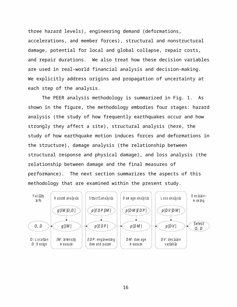
The PEER analysis methodology is summarized in Fig. 1. As shown in the figure, the

methodology embodies four stages: hazard analysis (the study of how frequently earthquakes

occur and how strongly they affect a site), structural analysis (here, the study of how earthquake

motion induces forces and deformations in the structure), damage analysis (the relationship

between structural response and physical damage), and loss analysis (the relationship between

damage and the final measures of performance). The next section summarizes the aspects of this

methodology that are examined within the present study.

10

g [IM |O ,D ]

g [IM ]

IM : in te n s itym e a su re

O , D Selec tO , D

H a z a rd a n a ly s is S tru c t 'l a n a ly s is

p [E D P |IM ]

p [E D P ]

E D P : e n g in e e r in gd e m a n d p a ra m .

O : L o c a tio nD : D e s ig n

D a m a g e a n a ly s is

p [D M |E D P ]

p [D M ]

D M : d a m a g em e a su re

L o ss a n a ly s is

p [D V |D M ]

p [D V ]

D V : d e c is io nv a r ia b le

D e c is io n -m a k in g

F a c il ityin fo

Fig. 1. Overview of PEER analysis methodology.

Intensity measures. Seismic intensity will be measured initially in terms of damped

elastic spectral acceleration response at the building’s small-amplitude fundamental period (Sa).

PEER researchers will also test alternative intensity measures (IM). Our objective is to identify

an IM that is more strongly correlated with performance, and whose occurrence rates can be

readily calculated. That is, the new IM should reduce uncertainty on facility performance,

conditioned on hazard level. We illustrate the calculation of probability (or occurrence rate)

p[IM], and a methodology for selecting and scaling ground motions with a desired IM. It would

desirable to create a probabilistic model of detailed ground motion as a function of IM, i.e.,

p[GM|IM], but for the present, we treat as equiprobable a set of historic ground-motions

recorded at similar sites with approximately similar hazard conditions.

Engineering demand parameters. PEER researchers will attempt to identify a limited

set of engineering demand parameters (EDP) that are indicative of overall structural response, for

use in simplifying design. It is hoped that a single parameter (or perhaps a small set) such as

peak transient drift at the top of the structure, will correlate strongly enough with performance

that structural designers will not need to explicitly evaluate damage and loss, but merely

demonstrate that EDP is less than some allowable level, associated with the desired level of

performance. We will elucidate and illustrate a methodology for calculating the conditional

probability p[EDP|GM, IM], and given this and p[GM|IM], the probability p[EDP|IM]. One can

convolve p[EDP|IM] with p[IM] to produce p[EDP], as illustrated in Fig. 1, or carry along

conditioning on IM until the end of the process, depending on how one wishes to express

performance.

11

Damage measures. PEER researchers will create or compile fragility functions for the

major damageable contents of the building. Fragility functions give the probability of a facility

component reaching or exceeding an undesirable performance level, as a function of excitation.

PEER researchers will categorize the building contents in a limited, clearly defined taxonomic

system; define relevant physical damage measures (DM) for each category; and create fragility

functions for each damage state, p[DM|EDP]. Given this and p[EDP], we will elucidate and

illustrate the calculation of p[DM]. Again, conditioning on IM can be carried though the

process, so the product of the damage analysis can also by p[DM|IM].

Decision variables. These decision variables (DV) measure overall facility performance

in terms most relevant to facility stakeholders. For the building owner considered here, DV is

most likely to include the operational failure of the scientific laboratories housed in the building.

This study elucidates and illustrates a methodology for calculating p[DV|DM] and, given p[DM],

the calculation of p[DV]. If one retains conditioning on IM, the product of this stage is

expressed as p[DM|IM], which represents the generic case of a seismic vulnerability function. It

can measure performance at discrete hazard levels, as in the ASCE/FEMA methodology. One

can then convolve with IM to produce p[DV], which can measure per-event, per-year, or lifetime

performance, depending on how hazard is expressed.

Decision-making implications. While financial decision-making is not a primary focus

of PEER’s effort, we recognize that to define and estimate DV correctly, we must understand

how the DV is used in financial practice. This study therefore examines the decision-making

practices of typical stakeholders of such a building, and illustrates how the DV estimates

produced here could inform an owner’s risk-management decisions.

Uncertainty. We identify the major sources of uncertainty in p[DV], quantifying the

contribution at each step from IM, GM, EDP, and DM to DV, considering propagation and

correlation. We identify the sources of uncertainty that are most significant in this situation, and

those that can be neglected. Of the major contributors, we identify opportunities for reducing

uncertainty by additional data-gathering or by changes in modeling. In other situations, such as a

similar commercial building on liquefiable soil, a newer building, or a bridge, different sources

of uncertainty may be more important. The larger PEER effort will seek to categorize a variety

of such situations and identify important sources of uncertainty in each.

12

2 Methodology Components to be Tested H. Krawinkler, G.G. Deierlein

2.1 CASE SPECIFIC SUMMARY OF METHODOLOGY

Global methodology (by reference – presumes that a methodology paper will be

available)

Components applicable to testbed

Major challenges

Deliverables:

Draft of chapter by November 30, 2003

Authors: Krawinkler, Cornell, Deierlein, Miranda, May

13

3 Hazard AnalysisP. Somerville, C.A. Cornell, S. Kramer

3.1 CONVENTIONAL FREE-FIELD HAZARD ANALYSIS AND GROUND MOTION

SELECTION

3.1.1 Seismic Hazard

Although the site is located near active faults in map view (i.e., when viewed from above,

the site is located near the traces of active faults), none of the faults that dominate the seismic

hazard at the site are oriented in such a way that the site will experience strong rupture directivity

effects. For example, the fault that caused the 1994 Northridge earthquake is located about 10

km below the site, but it dips up to the north-northeast and focuses forward rupture directivity

toward the northern part of the San Fernando Valley.

The longitudinal axis of the building is oriented east-west and the transverse axis is

oriented north-south. We used the east-west and north-south components of the recordings to

represent the longitudinal and transverse components of ground motion respectively. Recordings

of the Northridge earthquake from the northern San Fernando Valley and the Santa Clarita basin

are not suitable representations of the ground motions at the site, because they all contain strong

forward rupture directivity effects.

The site condition is classified as NEHRP category SD based on blow-count data. This

report describes ground motion time histories for SD soil conditions.

3.1.2 Uniform Hazard Spectra

Uniform hazard spectra for the site, listed in Table 1, were derived from the USGS

probabilistic ground motion maps for rock site conditions (Frankel et al., 1996, 2001).

Modification to account for near fault rupture directivity effects, and the use of separate response

spectra for the fault normal and fault parallel components of ground motion, is not be required,

for the reasons stated above.

14

Soil spectra were generated from the rock site spectra by multiplying the rock spectra by

the ratio of soil to rock spectra for the Abrahamson and Silva (1997) ground motion model.

These ratios are for the mode magnitude and distance combinations from the deaggregation of

the hazard, listed in Table 2.

Table 1. Equal-Hazard Response Spectra for the Van Nuys Building

Hazard level Period Rock Soil

50% in 50 yr 0.01 0.248 0.2320.1 0.422 0.3360.2 0.554 0.4910.3 0.522 0.5430.5 0.375 0.4790.8 0.24 0.341.0 0.188 0.2871.5 0.125 0.212.0 0.100 0.174

10% in 50 yr 0.01 0.628 0.4900.1 1.213 0.8190.2 1.434 1.0990.3 1.377 1.2760.5 1.125 1.3390.8 0.71 0.981.0 0.528 0.8061.5 0.32 0.532.0 0.235 0.420

2% in 50 yr 0.01 0.989 0.6980.1 1.898 1.1350.2 2.262 1.5590.3 2.200 1.8720.5 1.754 1.9800.8 1.37 1.671.0 0.945 1.4431.5 0.57 0.972.0 0.401 0.729

15

3.1.3 Deaggregation of the Hazard

The deaggregation of the hazard shows that the hazard at the site is dominated by nearby

earthquakes. The higher ground motions for the 2% in 50 year probability level than for the 10%

in 50-year level will reflect not larger magnitudes, but higher ground motion levels for the same

magnitude (larger number of standard deviations above the mean).

Table 2. Deaggregation of uniform hazard spectra, 5% damping, soil, east (transverse) Sa at 1 second, at the Van Nuys building

Hazard level Earthquake source Mean M Mean R

50% in 50 years Santa Susana, Northridge blind thrust 6.75 20 km

10% in 50 years Northridge blind thrust, Santa Susana 6.75 10 km

2% in 50 years Northridge blind thrust, Santa Susana 6.75 5 km

3.1.4 Record Selection.

The selected recordings were chosen to satisfy the magnitude and distance criteria from

the deaggregation, and the recording site criterion of SD. Additional criteria are that the

earthquake have a thrust mechanism, including blind thrust mechanisms (like the 1994

Northridge earthquake), and that the recording not contain strong forward rupture directivity

effects. All of the recordings are from thrust earthquakes in the Los Angeles region, and include

the 1971 San Fernando, 1986 North Palm Springs, 1997 Whittier Narrows, and 1994 Northridge

earthquakes. All of the selected recordings are from soil sites. Much better representations of

appropriate site effects could be made in the selection of time histories, for example by using

recordings from sites with comparable seismic velocity profiles, if there were seismic velocity

data at the site (as exists for the ROSRINE sites).

For each set of recordings, a scaling factor was found by matching the east component

time history to the longitudinal uniform hazard spectrum at a period of 1.5 sec. This scaling

factor was then applied to all three components of the recording. This scaling procedure

preserves the relative scaling between the three components of the recording.

16

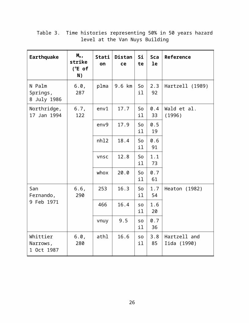
The time histories used to represent the 50% in 50 year ground motions are listed in

Table 3. These time histories are derived from the 1971 San Fernando, 1986 North Palm

Springs, 1987 Whittier Narrows, and 1994 Northridge earthquakes. The time histories used to

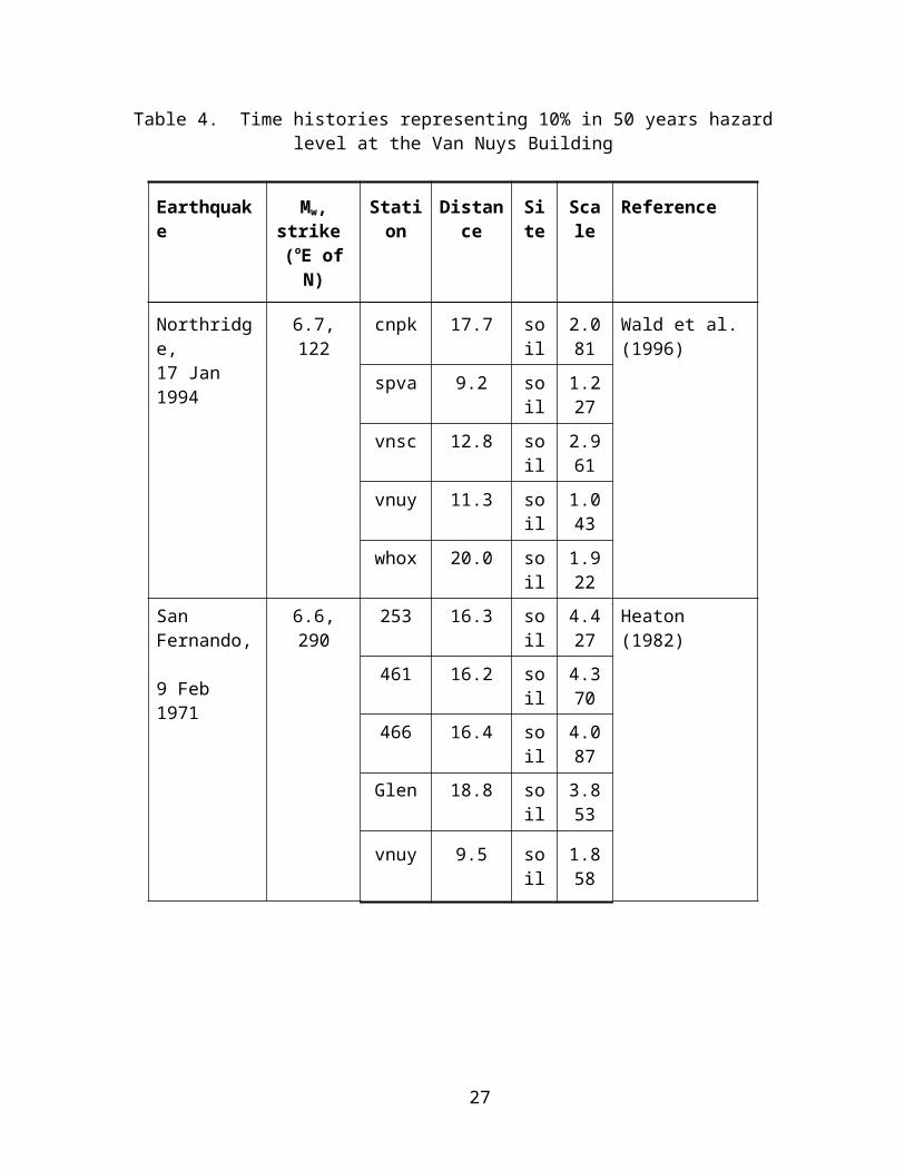
represent the 10% in 50 year ground motions are listed in Table 4. These time histories are

derived from the 1971 San Fernando and 1994 Northridge earthquakes. The time histories used

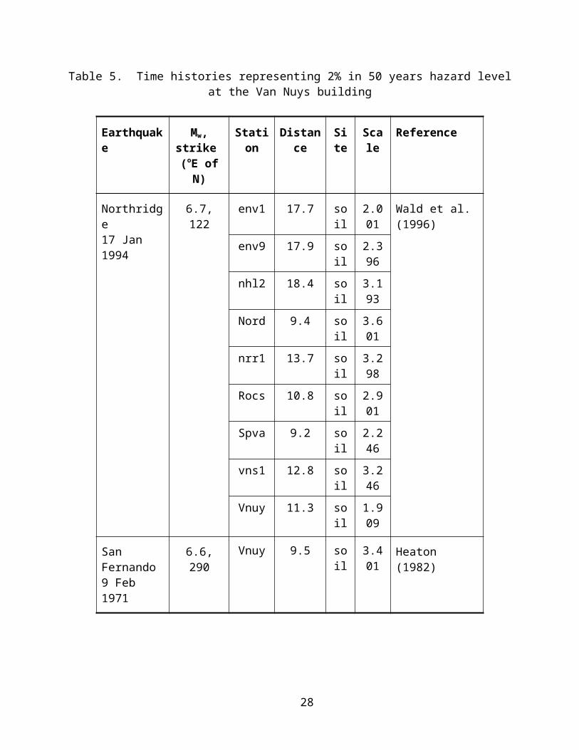
to represent the 2% in 50 year ground motions are listed in Table 5. With the exception of the

Van Nuys recording of the 1971 San Fernando earthquake, all of these time histories are from

the 1994 Northridge earthquake.

Table 3. Time histories representing 50% in 50 years hazard level at the Van Nuys Building

Earthquake Mw, strike

(oE of N)

Station Distance Site Scale Reference

N Palm Springs, 8 July 1986

6.0, 287 plma 9.6 km Soil 2.392 Hartzell (1989)

Northridge, 17 Jan 1994

6.7, 122 env1 17.7 Soil 0.433 Wald et al. (1996)

env9 17.9 Soil 0.519

nhl2 18.4 Soil 0.691

vnsc 12.8 Soil 1.173

whox 20.0 Soil 0.761

San Fernando, 9 Feb 1971

6.6, 290 253 16.3 Soil 1.754 Heaton (1982)

466 16.4 soil 1.620

vnuy 9.5 soil 0.736

Whittier Narrows,

1 Oct 1987

6.0, 280 athl 16.6 soil 3.885 Hartzell and Iida (1990)

17

Table 4. Time histories representing 10% in 50 years hazard level at the Van Nuys Building

Earthquake Mw, strike

(oE of N)

Station Distance Site Scale Reference

Northridge, 17 Jan 1994

6.7, 122 cnpk 17.7 soil 2.081 Wald et al. (1996)

spva 9.2 soil 1.227

vnsc 12.8 soil 2.961

vnuy 11.3 soil 1.043

whox 20.0 soil 1.922

San Fernando,

9 Feb 1971

6.6, 290 253 16.3 soil 4.427 Heaton (1982)

461 16.2 soil 4.370

466 16.4 soil 4.087

Glen 18.8 soil 3.853

vnuy 9.5 soil 1.858

18

Table 5. Time histories representing 2% in 50 years hazard level at the Van Nuys building

Earthquake Mw, strike

(oE of N)

Station Distance Site Scale Reference

Northridge 17 Jan 1994

6.7, 122 env1 17.7 soil 2.001 Wald et al. (1996)

env9 17.9 soil 2.396

nhl2 18.4 soil 3.193

Nord 9.4 soil 3.601

nrr1 13.7 soil 3.298

Rocs 10.8 soil 2.901

Spva 9.2 soil 2.246

vns1 12.8 soil 3.246

Vnuy 11.3 soil 1.909

San Fernando

9 Feb 1971

6.6, 290 Vnuy 9.5 soil 3.401 Heaton (1982)

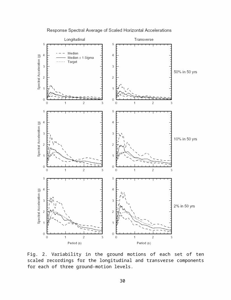
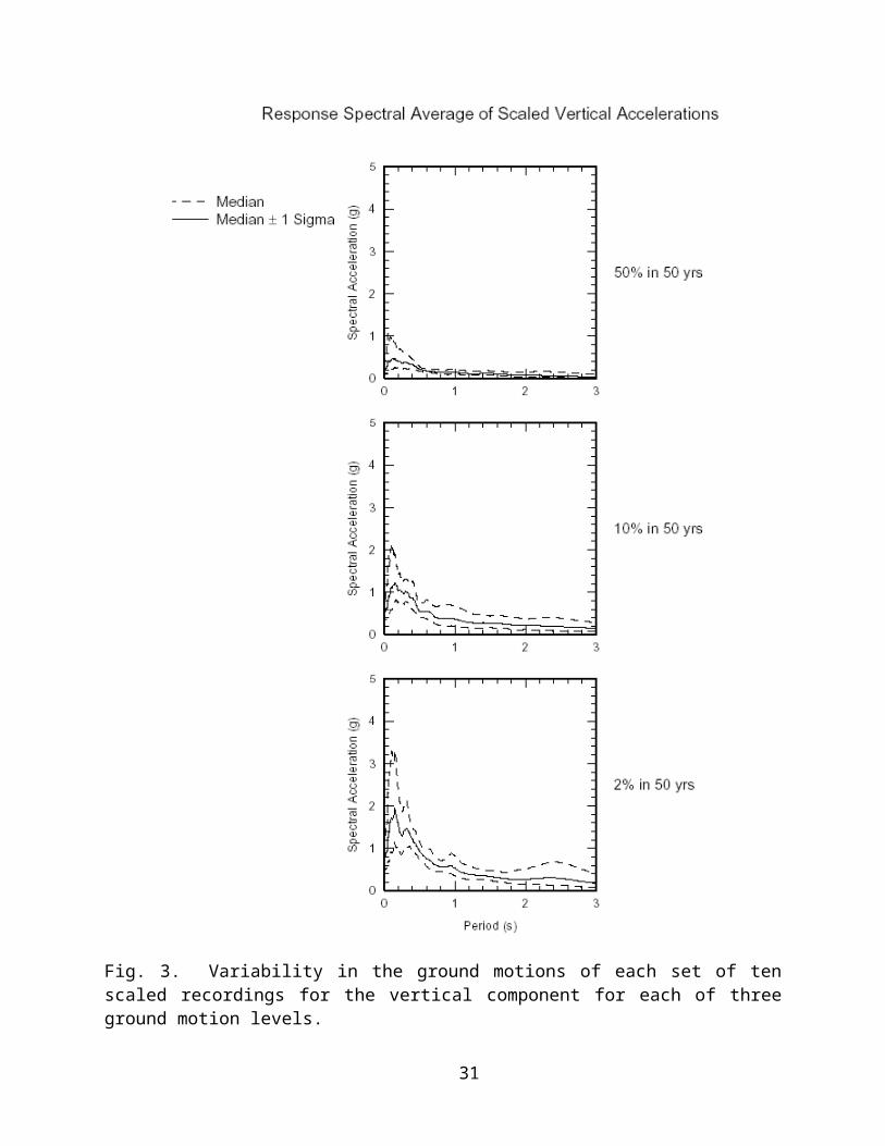
3.2 VARIABILITY IN THE GROUND MOTION RECORDINGS

The variability in the ground motion recordings for each component for each ground-

motion level is shown in Fig. 2 and Fig. 3 for the horizontal and vertical components,

respectively. These figures show the median and plus and minus one standard deviation level for

each set of ten recordings. The scaling causes the variability to go to zero for the longitudinal

component at 1.5 seconds.

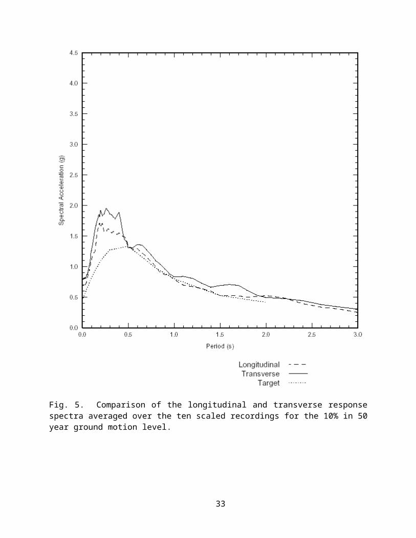
Comparison of Scaled Recording Spectra with the Uniform Hazard Spectra. Fig. 4,

Fig. 5, and Fig. 6 show the longitudinal and transverse response spectra averaged over the ten

recordings for the three ground motion levels. For all three ground motion levels, the average

response spectra of the longitudinal and transverse components of the recordings are similar to

each other, and they are also similar to the uniform hazard response spectra at periods longer

than 0.5 seconds. At periods shorter than 0.5 seconds, the average response spectra of the

recordings are larger than the uniform hazard spectra.

19

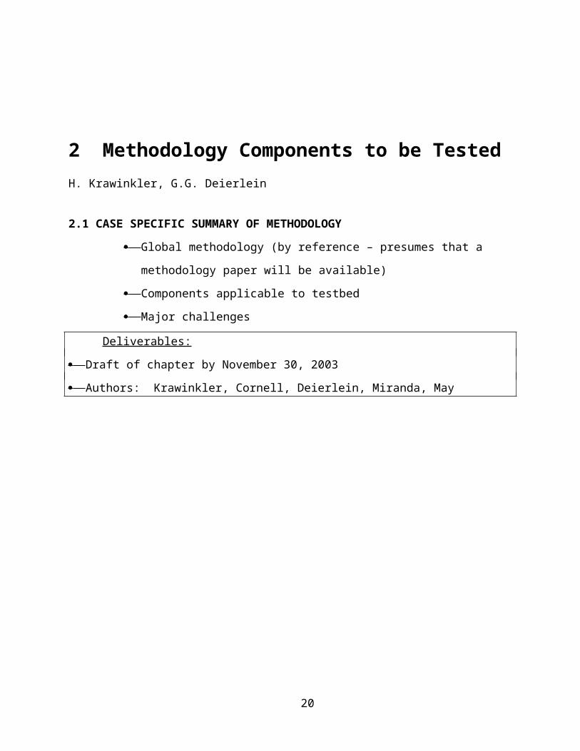
Fig. 2. Variability in the ground motions of each set of ten scaled recordings for the longitudinal and transverse components for each of three ground-motion levels.

20

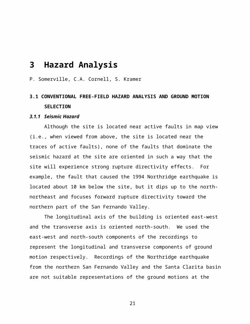
Fig. 3. Variability in the ground motions of each set of ten scaled recordings for the vertical component for each of three ground motion levels.

21

Fig. 4. Comparison of the longitudinal and transverse response spectra averaged over the ten scaled recordings for the 50% in 50 year ground motion level.

22

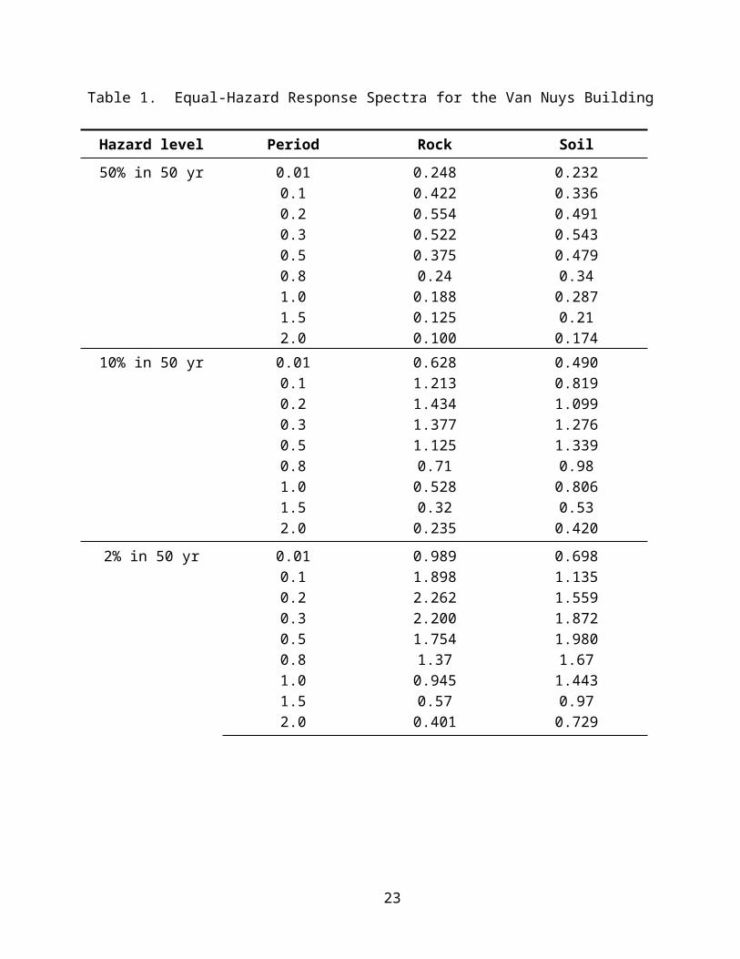
Fig. 5. Comparison of the longitudinal and transverse response spectra averaged over the ten scaled recordings for the 10% in 50 year ground motion level.

23

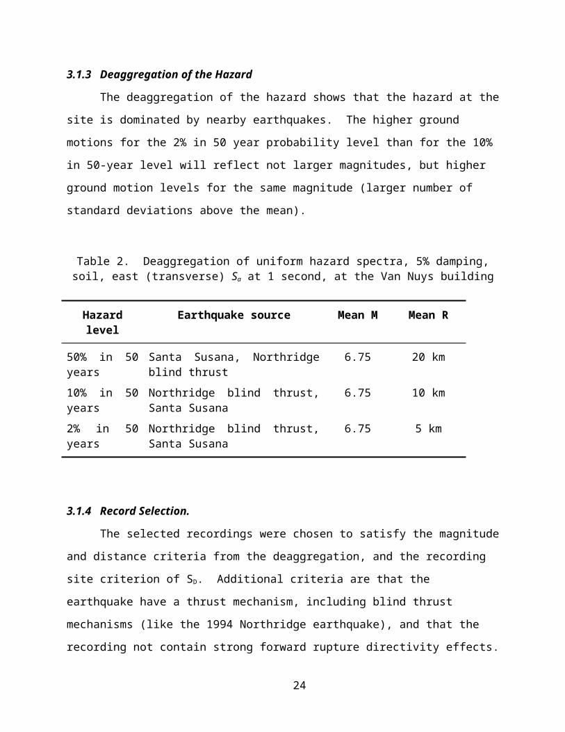
Fig. 6. Comparison of the longitudinal and transverse response spectra averaged over the ten scaled recordings for the 2% in 50 year ground motion level.

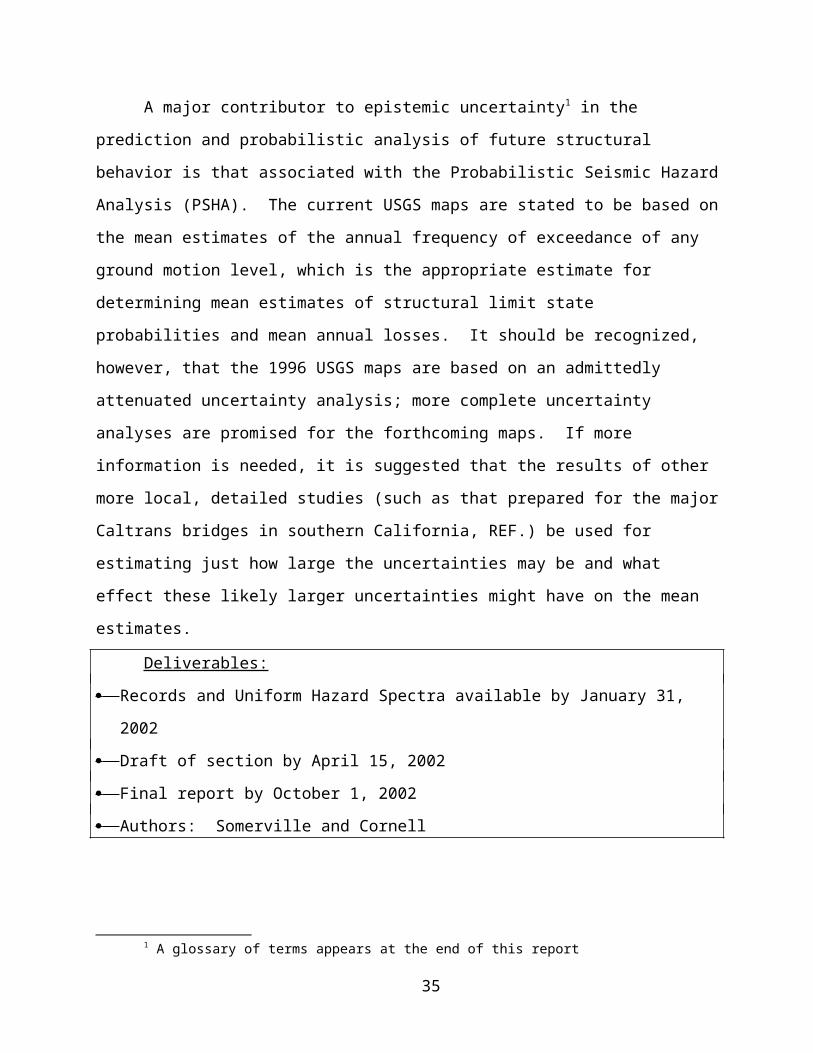
3.2.1 Epistemic Uncertainty in Probabilistic Seismic Hazard Analysis

A major contributor to epistemic uncertainty1 in the prediction and probabilistic analysis

of future structural behavior is that associated with the Probabilistic Seismic Hazard Analysis

1 A glossary of terms appears at the end of this report

24

(PSHA). The current USGS maps are stated to be based on the mean estimates of the annual

frequency of exceedance of any ground motion level, which is the appropriate estimate for

determining mean estimates of structural limit state probabilities and mean annual losses. It

should be recognized, however, that the 1996 USGS maps are based on an admittedly attenuated

uncertainty analysis; more complete uncertainty analyses are promised for the forthcoming maps.

If more information is needed, it is suggested that the results of other more local, detailed studies

(such as that prepared for the major Caltrans bridges in southern California, REF.) be used for

estimating just how large the uncertainties may be and what effect these likely larger

uncertainties might have on the mean estimates.

Deliverables:

Records and Uniform Hazard Spectra available by January 31, 2002

Draft of section by April 15, 2002

Final report by October 1, 2002

Authors: Somerville and Cornell

25

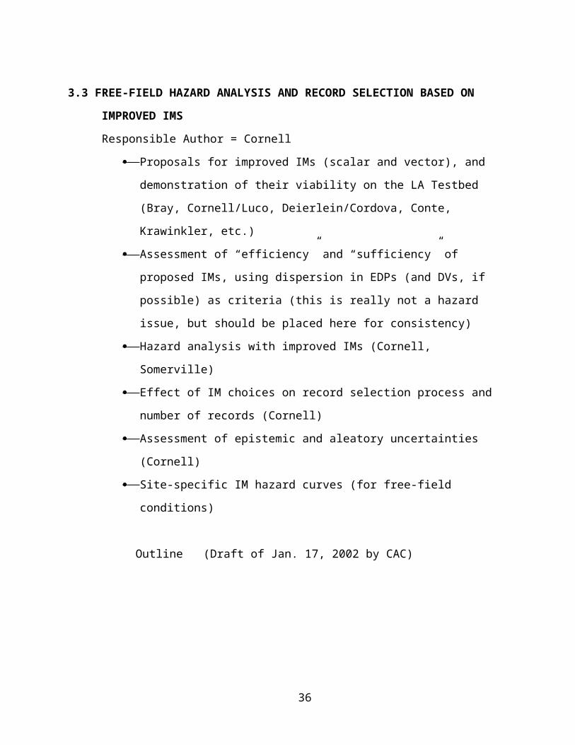
3.3 FREE-FIELD HAZARD ANALYSIS AND RECORD SELECTION BASED ON

IMPROVED IMS

Responsible Author = Cornell

Proposals for improved IMs (scalar and vector), and demonstration of their

viability on the LA Testbed (Bray, Cornell/Luco, Deierlein/Cordova, Conte,

Krawinkler, etc.)

Assessment of “efficiency” and “sufficiency” of proposed IMs, using dispersion

in EDPs (and DVs, if possible) as criteria (this is really not a hazard issue, but

should be placed here for consistency)

Hazard analysis with improved IMs (Cornell, Somerville)

Effect of IM choices on record selection process and number of records (Cornell)

Assessment of epistemic and aleatory uncertainties (Cornell)

Site-specific IM hazard curves (for free-field conditions)

Outline (Draft of Jan. 17, 2002 by CAC)

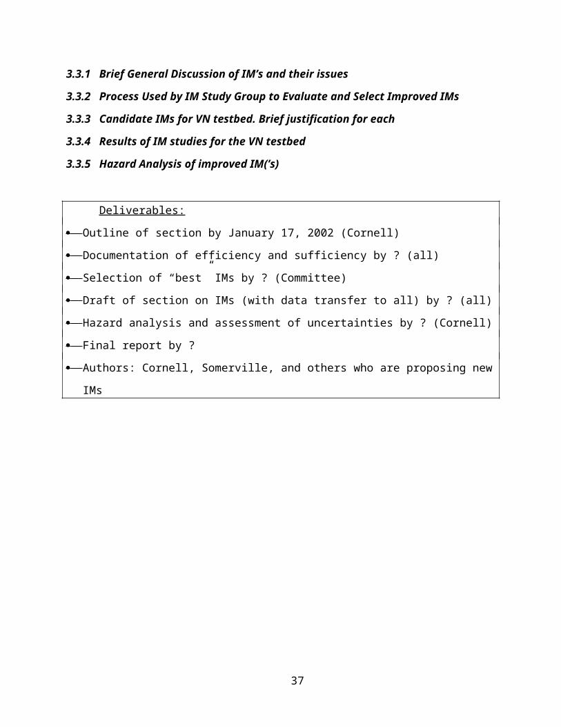
3.3.1 Brief General Discussion of IM’s and their issues

3.3.2 Process Used by IM Study Group to Evaluate and Select Improved IMs

3.3.3 Candidate IMs for VN testbed. Brief justification for each

3.3.4 Results of IM studies for the VN testbed

3.3.5 Hazard Analysis of improved IM(’s)

Deliverables:

Outline of section by January 17, 2002 (Cornell)

Documentation of efficiency and sufficiency by ? (all)

Selection of “best” IMs by ? (Committee)

Draft of section on IMs (with data transfer to all) by ? (all)

Hazard analysis and assessment of uncertainties by ? (Cornell)

Final report by ?

Authors: Cornell, Somerville, and others who are proposing new IMs

26

3.4 EFFECTS OF SITE SOIL PROFILE ON IMS AND GROUND MOTIONS

Responsible Author = Kramer

Best location for IMs and records (free-field versus foundation versus “bedrock”,

etc.) (Kramer, Kutter, Martin)

Effect of soil profile on IMs and records (Kutter, Martin, Kramer, Nagaa). Per

PEER methodology, where do you start the ground motion? Bruce has short

writeup.

Effect of soil profile on response of structure (soil-foundation-structure system) –

interaction with 4.1 (Kramer, Kutter, Martin, Nagaa)

Propagation of uncertainties due to soil properties (Kramer). Kramer’s tornado

diagram.

Deliverables:

Outline of section by January 17, 2002 (Kramer)

Model of soil profile by March 15 (Martin)

Records modified for site soil by April 15 (Martin, Kutter)

Assessment of soil-foundation-structure interaction by September 2002 (Kutter, Martin)

Draft of section by October 1, 2002

Final report by December 2002

Authors: Kramer, Kutter, Martin

Kramer’s outline of Section 3.4, of ~1 June 2002

Soil Conditions Kramer

Regional geology

Site investigations

Soil layers – thicknesses, properties, depth to bedrock

Groundwater conditions

Uncertainty, spatial variability

Foundation Conditions [moved to Section 4.1] Kramer

Site Response Kutter

Development of ground motions

Use of nearby ground motions

27

Use of site-specific response analyses

Optimum location for IMs/records

Effects of soil profiles on IMs/records

Soil-Foundation-Structure Interaction Martin

Introduction

Review of options

Discrete model

Spring constants

Translational DOFs

Rotational DOFs

Dashpot coefficients

Translational DOFs

Rotational DOFs

Effects of nonlinearities

Effects of uncertainties

Finite element model

Soil model

Pile model

Interface model

Pile cap model

Grade beam model

Modeling connections

Effects of uncertainties

Effects of Soil-Foundation-Structure Interaction on IMs Martin, Kutter

28

4 Prediction of EDPsL. Lowes, T. Hutchinson

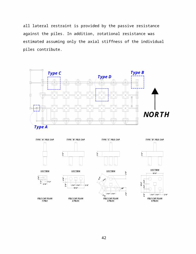
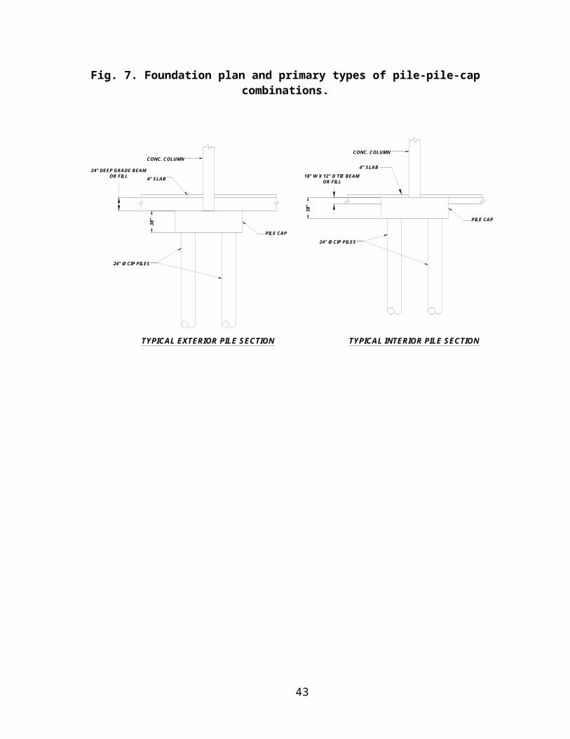
4.1 ANALYTICAL MODELING OF FOUNDATION

The supporting foundation below the Van Nuys building is a series of friction piles integrated

with pile caps as shown in Fig. 7. There are approximately four different types of pile-pile-cap

arrangements, ranging from single piles at select perimeter locations to 4 pile-groups. Pile and

pile-groups are nominally integrated with 24” deep gradebeams at the perimeter of the building

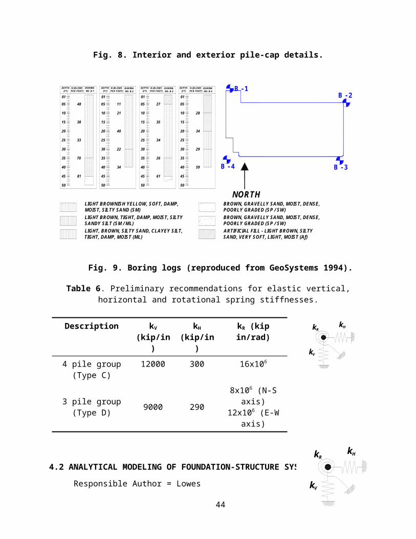
and 12” deep tie beams at the interior as shown in Figure 2. A geotechnical report prepared by

GeoSystems (1994) indicates primarily medium dense silty sands at the site as shown in the four

boring logs reproduced in Figure 3.

For preliminary seismic demand assessment, the foundation actions may be approximated by

uncoupled elastic spring components representing vertical, horizontal and rotational resistances.

Using the methodology suggested in FEMA 273/274 (1997) and an estimated friction angle of ’

= 35º, elastic spring resistances have been estimated and are provided in Table 1. Such

estimations are based on the assumption that the pile-pile-cap connection provides no rotational

restraint (i.e. pinned) and that base contact at the pile-cap is negligible, thus all lateral restraint is

provided by the passive resistance against the piles. In addition, rotational resistance was

estimated assuming only the axial stiffness of the individual piles contribute.

29

NORTH

Type CType D

Type B

Type A

PILE CAP PLAN4 PILES

SECTIONSECTION

PILE CAP PLAN3 PILES

SECTION

PILE CAP PLAN2 PILES

3'-0

"3'

-0"

2'-0

"

10'-0

"

3'-0" 2'-0"3'-0" 3'-0"2'-0"

2'-0"6'-0"

2'-0

"2'

-0"

60°

3'-0" 3'-0" 2'-0"10'-0"

2'-0

"4'

-0"

1'-3

"2'

-6"

1'-3"2'-6"

SECTION

PILE CAP PLAN1 PILE

TYPE "A" PILE CAP TYPE "B" PILE CAP TYPE "C" PILE CAP TYPE "D" PILE CAP

10'-0"

3'-0"

3'-2

"

3'-2

"

3'-2

"

Fig. 7. Foundation plan and primary types of pile-pile-cap combinations.

30

4" SLAB

CONC. COLUMN

24" Ø CIP PILES

PILE CAP

24" DEEP GRADE BEAM OR FILL

CONC. COLUMN

18" W X 12" D TIE BEAM OR FILL

24" Ø CIP PILES

PILE CAP

4" SLAB

38"

38"

TYPICAL EXTERIOR PILE SECTION TYPICAL INTERIOR PILE SECTION

Fig. 8. Interior and exterior pile-cap details.

Fig. 9. Boring logs (reproduced from GeoSystems 1994).

01

05

10

20

15

30

25

40

35

50

45

LIGHT BROWNISH YELLOW, SOFT, DAMP, MOIST, SILTY SAND (SM)LIGHT BROWN, TIGHT, DAMP, MOIST, SILTY SANDY SILT (SM / ML)

BROWN, GRAVELLY SAND, MOIST, DENSE, POORLY GRADED (SP / SW)

LIGHT, BROWN, SILTY SAND, CLAYEY SILT, TIGHT, DAMP, MOIST (ML)

ARTIFICIAL FILL - LIGHT BROWN, SILTY SAND, VERY SOFT, LIGHT, MOIST (Af)

BORING NO. B-1

N (BLOWS PER FOOT)

48

38

33

70

81

BORING NO. B-2

11

21

40

22

34

BROWN, GRAVELLY SAND, MOIST, DENSE, POORLY GRADED (SP / SW)

BORING NO. B-3

27

35

34

26

61

BORING NO. B-4

28

34

29

59

DEPTH(FT)

50

15

40

45

35

25

30

20

10

01

05

50

15

40

45

35

25

30

20

10

01

05

50

15

40

45

35

25

30

20

10

01

05

DEPTH(FT)

N (BLOWS PER FOOT)

DEPTH(FT)

N (BLOWS PER FOOT)

DEPTH(FT)

N (BLOWS PER FOOT)

B - 4

B - 1

B - 3

B - 2

NORTH

31

Vk

kHRk

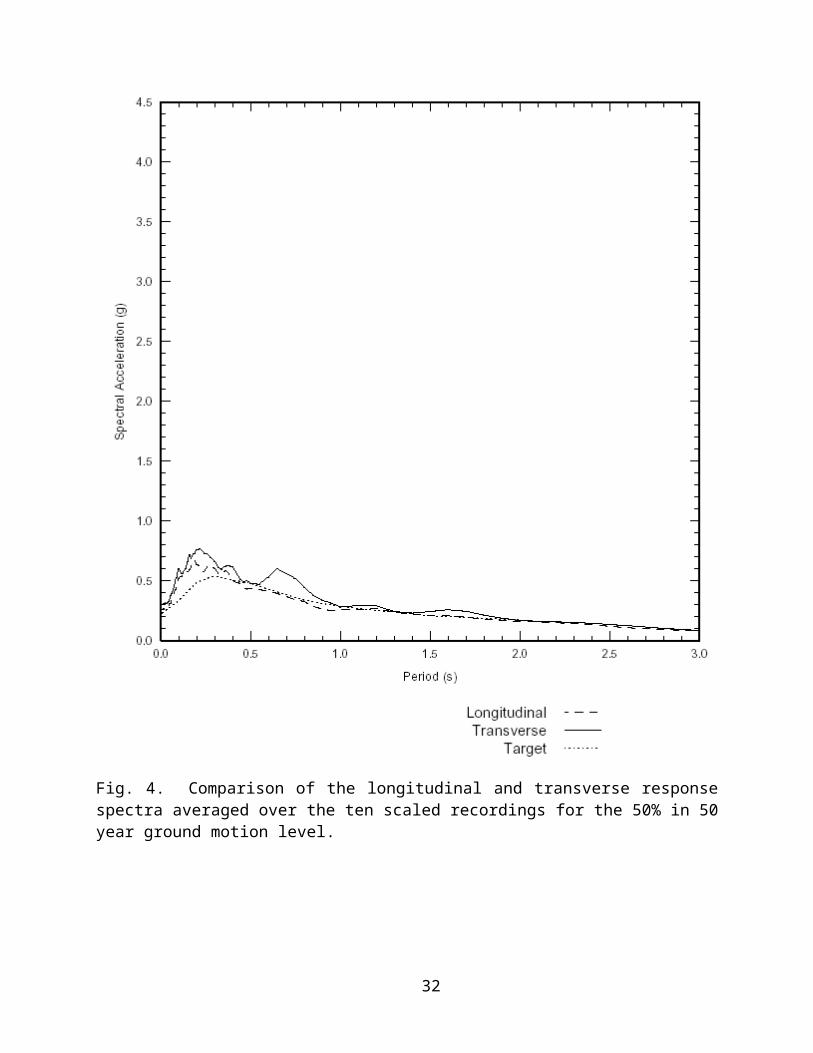
Table 6. Preliminary recommendations for elastic vertical, horizontal and rotational spring stiffnesses.

Description kV (kip/in) kH (kip/in) kR (kip in/rad)

Vk

kHRk4 pile group (Type C) 12000 300 16x106

3 pile group (Type D) 9000 2908x106 (N-S axis)

12x106 (E-W axis)

4.2 ANALYTICAL MODELING OF FOUNDATION-STRUCTURE SYSTEM

Responsible Author = Lowes

Modeling of element behavior (with deterioration) (Lowes, Deierlein)

Utilization of Structural Performance Data Base (Fenves)

Modeling of foundation components (Martin, Lowes)

Modeling of soil-foundation interface (Martin, Kutter, Sitar)

There is much coordination needed between researchers on the previous four

bullets (Lowes, Deierlein, Fenves, Martin, Kutter, Sitar)

Impact of modeling complexity on a few EDPs: max PTD, max PDA, max roof

displacement. Linear response spectrum, multiple nonlinear pushover models,

multiple nonlinear time-history structural analyses.

Impact of modeling assumptions on uncertainties. HK: effect of model

parameter uncertainties on period by Oct 1 Lowes. Lowes: effect of

uncertainties in damping, hinge length, etc., on EDP.

One paragraph saying, only did 2D modeling for good reasons.

Draft outline by L. Lowes (1/17/02)

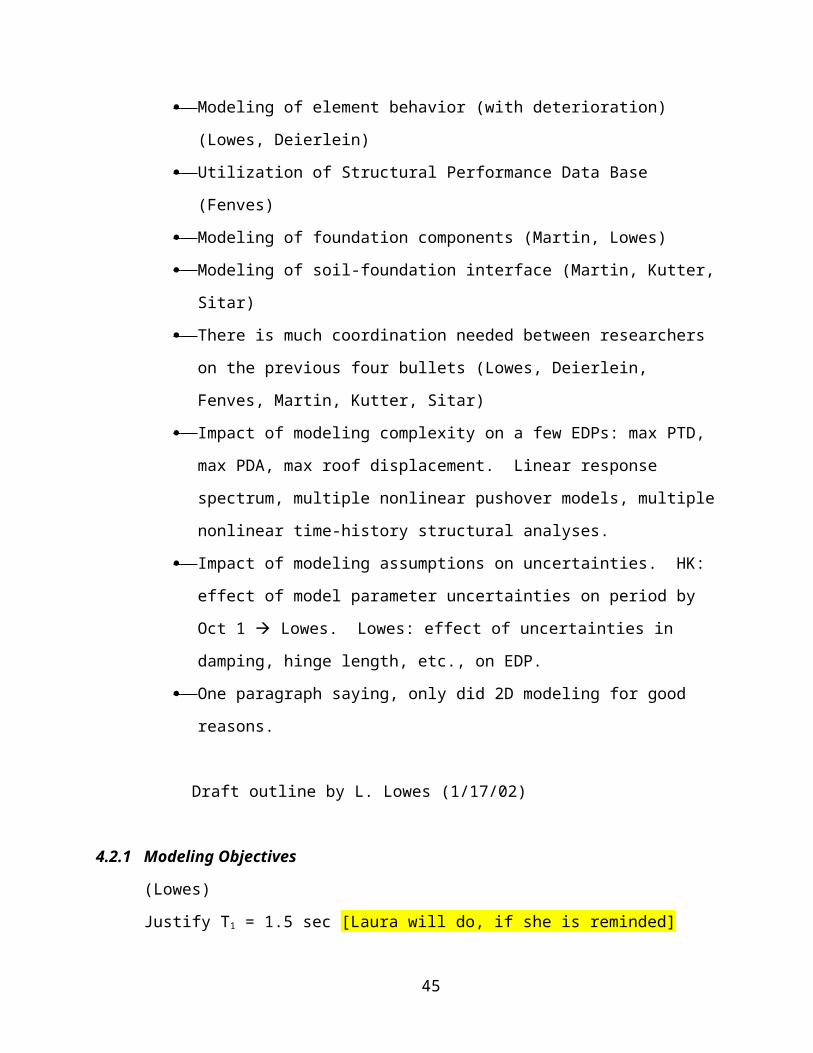
4.2.1 Modeling Objectives

(Lowes)

Justify T1 = 1.5 sec [Laura will do, if she is reminded]

Present D, V, A at floor levels, [story displacement time histories], M-q at beam-column

sections, total joint deformation.

32

4.2.1.1 Efficiency

4.2.1.2 Flexibility

4.2.1.3 Accuracy

4.2.1.4 Calculation of EDP’s

4.2.2 Types of Models Employed

4.2.2.1 Modeling assumptions

(Lowes)

4.2.2.2 2D vs. 3D

(Lowes)

4.2.2.3 Element formulations

(Lowes, Deierlein)

Traditional elements

Non-ductile beam-column element

Beam-column joint element

Foundation elements

4.2.2.4 Modeling of the soil-foundation interface

(Sitar, Kutter, Martin)

4.2.3 Model Verification

4.2.3.1 Structural performance database

(Fenves)

4.2.3.2 Verification of structural elements

(Lowes)

4.2.3.3 Verification of foundation elements and soil-foundation model

(Sitar, Kutter, Martin)

4.2.3.4 Verification of structure response through comparison with sensor data

(Lowes)

4.2.4 Results

4.2.4.1 Typical simulation results

(Lowes)

4.2.4.2 The impact of modeling assumption on model uncertainty

(??)

33

Deliverables:

Outline of section by January 17, 2002 (Lowes)

First 2-D structural model of structure-foundation system by February 28, 2002 (with transfer

of OpenSees model and documentation to other researchers), with improved models to

follow. Work on 2-D modeling of original structure to be completed by May 2002 (Lowes)

Design of retrofitted structure by Heintz by August 31, 2003.

2-D models (one by Heintz, one by Lowes) of retrofitted structures. Heintz by 31 Au 2003,

Lowes by 15 Oct 2003. Lowes’ will use beam-column elements for the shearwall, and input

the same 30 records and provide EDPs. Added effort outside of present scope is creation by

Miranda of fragility functions, perhaps using FEMA 306, 307, 308, and loss model by 15 Oct

2004.

Draft by 10/15/03

Final draft by 12/31/03

Authors: Lowes, Deierlein, Fenves, Sitar, Kutter, Martin

34

4.3 VALIDATION OF ANALYTICAL MODELS

Responsible Author = Lowes

Validation through component tests (Lehman, Lowes, Stanton, Moehle) (by

October 2002). Subassemblage tests considering simulated and observed

response, focusing on columns and joints, using simple (nonductility-based)

column shear-failure models.

Validation through frame tests (Moehle) (by October 2003?) Krawinkler will

follow up with Moehle on this.

Draft outline by L. Lowes (1/17/02)

4.3.1 Experimental Data Used in Model Development and Validation

(October 2002)

4.3.1.1 Beam-column joint data

(Lehman, Lowes, Stanton)

4.3.1.2 Non-ductile column data

(Moehle and Wallace?)

4.3.1.3 Data from frame tests

(Moehle by October 2003?)

4.3.2 Validation Protocol

(Lowes)

4.3.2.1 Load histories considered in model verification

4.3.2.2 Quantification of model accuracy and precision

4.3.2.3 Simulation of response

4.3.3 The EDP to DM Relationship

4.3.4 Structural Performance Data Base

(Fenves)

Deliverables:

Outline of section by January 17, 2002 (Lehman, Moehle)

Draft on component validation tests by October 2003

35

Draft on frame validation test by October 2003

Final report by December 2003

Authors: Moehle, Lehman, Lowes, Stanton

36

4.4 PREDICTION OF EDPS FOR DAMAGE ASSESSMENT

Responsible Author = Miranda

Name the relevant EDPs for damage assessment, including structural,

architectural, MEP, and content subsystems (Miranda, with contributions by

Lowes, Porter, Eberhard, Stanton, and Lehman. Lowes will tell Stanton and

Lehman that they are responsible)

Predictions of EDPs from non-deteriorating and deteriorating models (e.g.,

structure specific descriptions of EDP/IM, and site-specific EDP hazard curves)

(Cornell, Krawinkler, Miranda. EDP data from Lowes by 7 Jul 2003. Miranda

suggests complete text by 15 Sep 2003)

Propagation of uncertainties (this ties in with Section 4.2) (Cornell, Kramer,

Miranda) Chapter 6?

Sensitivities by OpenSees? (Der Kiureghian, Conte – not officially on team)

Prediction of EDP by means of simplified engineering approaches e.g., by

pushover (Krawinkler by 30 Nov 2003)

Outline

4.4.1 General discussion of the role of EDP’s in the methodology

4.4.2 Selection of EDP Vector

(Prepared by EM for insertion in section 4.3)

The Engineering Demand Parameters (EDP’s) that are being considered (by Eduardo and

his students) in connection to PEER’s efforts in loss estimation methodology as applied to the

Van Nuys testbed are:

1. Interstory Drift Ratio (IDR)

2. Peak Absolute Floor Acceleration (PFA)

3. Peak Absolute Floor Velocity (PFV)

The first type of EDP is being evaluated at all story levels while the second and third

types of EDPs are being evaluated at all floor levels including the ground floor level. Hence

these EDPs represent a vector of 23 scalar quantities of peak structural motion (peak structural

response parameters). It is important to note that these EDPs represent peak (maximum absolute

values) of these response parameters and do not necessarily occur at the same time.

37

Interstory drift ratio (IDR) is closely correlated with structural damage of all elements

present in this building, e.g. columns, spandrel beams, slabs and their corresponding connections.

IDR is also well correlated with damage to many types of nonstructural components. A few

examples are: masonry infill walls, interior partitions, windows and glazed walls, interior and

exterior doors, staircases, railings in the elevator, elevator doors, vertical piping, etc.

Peak absolute (ground plus relative) floor acceleration (PFA) is closely correlated with

damage to other nonstructural elements, such as: parapets, suspended ceilings, fire sprinklers,

electrical power generators, counterweights in elevator, horizontal piping, air conditioning units,

etc. Damage to some types of contents may also be correlated to PFA.

Peak absolute (ground plus relative) floor velocity is correlated with damage to some

types of contents (particularly those susceptible to overturning).

It has been shown (Aslani and Miranda, 2002) that the above engineering demand

parameters can be assumed to be lognormally distributed at any given level of intensity, for the

range of intensity measures that are of interest in this testbed. The lognormal probability

distribution only requires two parameters to be fully defined. One parameter is a measure of

central tendency and the other is a measure of dispersion. There are many possible ways to

estimate these parameters. For a detailed discussion on different alternatives for these two

parameters of the lognormal probability distribution the reader is referred to Aslani and Miranda,

2002.

The alternatives that have been considered for the measure of central tendency are:

(i) The exponential of the mean of the natural log of the data; XLne

(ii) The sample (i.e., counted) median;

(iii) A measure of central tendency computed from a regression analysis in normal

coordinates; r~ (for details see Aslani and Miranda 2002).

The alternatives being considered for measure of dispersion are:

(i) The standard deviation of the natural log of the data; XLn

(ii) A measure of dispersion calculated based on the inter-quartile range of the data; (for details see Aslani and Miranda 2002).

(iii) A measure of dispersion calculated based on a regression analysis in normal

coordinates; r~ (for details see Aslani and Miranda 2002).

38

The following recommendations can be made on the applicability of the above

alternatives for the measure of central tendency and of dispersion:

(i) If the EDP’s calculated from time history analyses do not include values that are

significantly larger than the rest of the sample (values that can be considered as

outliers) then XLne and XLn can be used as the measures of central tendency and

dispersion, respectively.

(ii) If the EDP’s calculated from the time history analyses include outliers, but the

sample size is large enough (including results of 10 or more ground motions) then

the counted median of the data can be used as a better measure of central

tendency and calculated from the inter-quartile range of the data can be used as

a better measure of dispersion. This situation arises for example when looking at

IDR in certain floors where computed values for certain ground motions can be

extremely large (collapse cases).

(iii) If the EDP’s calculated from the time history analyses include outliers and the

sample size is small (including less than 10 data points) then the parameters

calculated from the regression analysis, r~ and r~ , are recommended as more

reliable measures of central tendency and dispersion for most of the data in the

sample.

In the approach proposed by Aslani and Miranda 2002, the variation of the measures of

central tendency and dispersion are describe by continuum functions given by:

For the measure of central tendency:

3)(~21

IMIMr (Eq 1)

For the measure of dispersion:

2321 )()(

1~IMIM

r

(Eq 2)

where IM is the selected intensity measure, 1, 2 , 3 are constants are constants that are

computed from a regression analysis with three known IM - r~ pairs. Parameters 1, 2 , and 3

are constants that are computed from a regression analysis with three known IM - r~ pairs.

Therefore in the approach proposed by Aslani and Miranda measures of central tendency and

dispersion are evaluated at three levels of intensity measure. For details on the selection of these

ground motion intensity levels the reader is referred to Aslani and Miranda, 2002. Please note

39

that unlike the LRFD-format simplified approach proposed by Cornell et al. for SAC, here the

dispersion is NOT assumed constant, its variation is explicitly captured.

4.4.3 Results of EDP versus IM

4.4.4 EDP Hazard Curves

4.4.5 Epistemic Uncertainty.

Effect of this on EDP hazard curves.

4.4.6 Prediction by Means of Simplified Approaches

(results from generic structures, various analysis methods [elastic, pushover]

Deliverables:

Draft by October 15, 2003

Final draft by December 31, 2003

Authors: Miranda, Cornell, Krawinkler, Kramer (Der Kiureghian & Conte?)

4.5 PREDICTION OF COLLAPSE PROBABILITY

Responsible Author = Krawinkler

Models for global and local collapses (Lowes, Krawinkler (generic models),

Moehle (columns), Miranda (flat plates), Deierlein (OpenSees), Fenves

(OpenSees)).

Prediction of global and local collapses, and assessment of collapse modes

(Lowes, Cornell, Krawinkler, Moehle)

4.5.1 Discussion of Collapse Estimation and its Role in Method

4.5.2 Models for Global and Local Collapse

4.5.3 Results of Collapse Predictions

4.6 ESTIMATION OF CASUALTIES

4.6.1 Theoretical Means

Cornell’s approach; text by Cornell

4.6.2 Prediction by Means of Simplified Approaches

(results from generic structures, approximate analysis methods [pushover])

Prediction of casualties (Cornell)

40

Propagation of uncertainties (Cornell, Krawinkler)

Prediction by means of simplified engineering approaches (Krawinkler)

Loss modeling: P[collapse | IM] (from Krawinkler 31 Aug 2003; from

Miranda…), p[Death | occupant] (from Seligson by 31 Aug 2003), p[occupant]

(from Seligson by 15 Jul, assuming Porter provides contact info by 1 Jul) Loss

model done by Miranda by 15 Oct 2003.

Deliverables:

Outline of section by January 17, 2002 (Krawinkler)

Global collapse predictions by October 1, 2002 (Lowes, Krawinkler, Cornell)

Partial draft by October 2002

OpenSees model for local collapse (M-P-V) & propagation by October 1, 2002 (Deierlein,

Lowes, Fenves)

Local collapse prediction and consequences by April 2003 (??)

Final report by May 2003

Authors: Krawinkler, Cornell, Lowes, Deierlein, Fenves

41

5 Prediction of Losses

5.1 DM/EDP AND DV/DM RELATIONSHIPS

… for Important Structural and Nonstructural Components

Responsible Authors = Miranda (nonstructural) + Lowes (structural)

The DM refers to a limit state that requires remedial action (e.g., replacement of

a gypsum board wall), and the DM/EDP relationships may be viewed as

“fragility” curves

Determine “realistic” DM/EDP and DV/DM relationships for selected structural,

architectural, MEP, and content components/subsystems (Miranda), see Section

5.3. The DV should be $ losses

Draft outline by E. Miranda (1/16/02)

5.1.1 Structural Elements

(Lowes and Miranda)

5.1.1.1 Beam-Column Connections

(Lowes w/input from Stanton/Lehman by 31 Aug 2003)

P(DM|EDP) of beam-column connections

P(DV|DM) of beam-column connections

5.1.1.2 Slab-Column Connections

(Miranda w/input from Moehle/Roberston by 15 Aug 2003.)

P(DM|EDP) of slab-column connections

P(DV|DM) of slab-column connections

5.1.1.3 Columns

(Miranda w/ significant input from Moehle by 15 Oct 2003.)

P(DM|EDP) of columns

42

P(DV|DM) of columns

5.1.2 Nonstructural Elements

(Miranda by 15 Oct 2003)

5.1.2.1 Drift Sensitive Nonstructural Components

(3 or 4 components)

P(DM|EDP) of drift sensitive non-structural components

P(DV|DM) of drift sensitive non-structural components

5.1.2.2 Slab-Column Connections

(Miranda w/input from Moehle/Roberston)

P(DM|EDP) of slab-column connections

P(DV|DM) of slab-column connections

(Prepared by EM for insertion in section 5)

The following damage states have been proposed for the slab-column connections based

on the experimental reports from other researchers:

1. Small cracking of the connection. This level of cracking typically represents crack

widths smaller than 0.2 mm associated with opening and closure of cracks.

2. Wide cracking of the connection. This damage state can be considered as the first

damage state at which the connection needs to be repaired.

3. Punching shear failure of the connection. At this damage state large cracking,

crushing and spalling of concrete surrounding the column occurs resulting in the

connection looses a significant portion of its lateral loading capacity.

4. Loss of vertical carrying capacity.

There is very little information available to develop EDP to DM functions of

nonstructural elements. In this research, the fragility curves are being developed based on three

different sources of information: (1) experimental results, (2) performance of nonstructural

components in instrumented buildings during previous earthquakes where damage reports are

available, (3) performance of nonstructural components during previous earthquakes in non-

instrumented buildings where damage reports are available.

5.1.2.3 Columns

(Miranda w/ significant input from Moehle)

P(DM|EDP) of columns

43

P(DV|DM) of columns

Deliverables:

Outline of section by January 17, 2002 (Miranda)

Select and describe components and limit states by March 15 (Miranda)

Quantify and disseminate DM/EDP and DV/DM relationships by July 15 (Miranda) (see EM

comments above)

Drafts of section by August 15, 2002.

Final report by October 1, 2002

Author: Miranda & Lowes

44

5.2 APPLICATION OF LOSS ESTIMATION METHODOLOGY

Responsible Author = Miranda/Porter

Summarize options in loss (downtime) estimation methodology (mean annual

losses, losses associated with specified earthquake levels (50/50, 10/50, 2/50?)

(e.g., how to integrate over all components of structure) (Miranda)

Alternative ways to formulate the decision variables, to better accommodate the

needs of owners (interaction with Chapter 8) (all)

Illustrate application of methodology to

o Pre-Northridge building

o Retrofitted building

o Building designed according to PEER methodology

Identify the major contributors to losses (structural vs. nonstructural)

Can the (DM/EDP + DV/DM) detour be avoided by providing cost functions that

directly relate EDP to DV? (Miranda)

Deliverables:

Outline Section by January 17, 2002 (Miranda)

Provide summary of methodology by March 15, 2002 (Miranda)

Itemize (quantity and location of) structural, architectural, MEP, and content

components/subsystems that will be considered in application by May 15, 2002 (Miranda)

Apply methodology to pre-Northridge building by October 1, 2002, with report (Miranda)

Apply methodology to retrofitted building by April 30, 2003, with report (Miranda, in

collaboration with retrofit designer [see Appendix B])

??Apply methodology to PEER designed building by June 30, 2003, with report (Miranda, in

collaboration with PEER methodology designer [see Appendix C])??

This issue is under discussion, because the effort on design methodology has not yet

started.

Final report by end of July 2003

Author: Miranda

45

(Prepared by EM for insertion in section 5.2)

Up to this point our efforts have been aimed at computing the expected annual loss in the

structure.

The expected value of the loss in component j (either a structural or nonstructural

component) is computed as:

dIMdEDPdIM

IMdimIMedpEDPPedpEDPdmDMPdmDMEEm

ijjiijj )()|( )|( ]|[$][$

1 0 0

(Eq

3)

where

m is the number of damage states in component j.

]|[$ ij dmDME is the expected value of the loss in component j given that it is in damage state i.

)|( edpEDPdmDMP ji is the probability that component j will be in damage state i given that component j has been subjected to an EDP equal to edp.

)|( imIMedpEDPP j is the probability that the EDP that affects component j will exceed a certain value edp given that the ground motion intensity measure IM is equal to im

dIMIMd )(

is the slope of the seismic hazard curve corresponding to the intensity

measure IM

The probability that component j will be in damage state i given that component j has

been subjected to an EDP equal to edp is computed as

)|()|()|( 1 edpEDPdmDMPedpEDPdmDMPedpEDPdsDMP jijjijjij (Eq 4)

where

)|( edpEDPdmDMP jij is the probability of exceeding damage state i in component j given that it has been subjected to an EDP equal to edp

)|( 1 edpEDPdmDMP jij is the probability of exceeding damage state i+1 in component j given that it has been subjected to an EDP equal to edp

The expected annual loss for the whole building, without considering downtime, is given

the sum of the expected losses in each individual component in the building, that is

46

n

jjnjjjjBldg EEEEEE

1321. $][$...][$][$][$][$ (Eq 5)

where n is the number of components in the building.

47

6 Propagation of Uncertainties from IM to DVResponsible Author = Porter. By 15 Oct 2003. I will ask Ufuk if he will write a few

pages on what you do with the DVs in financial modeling.

Identify and quantify all sources of uncertainties.

Propagate uncertainties and evaluate their impact on performance assessment

Identify important sources of uncertainty

The Uncertainty breakout group of 1/16/02 has written a draft that discusses the

uncertainty issues in some detail. This draft is available from H.K.

Deliverables:

Outline of section by January 17, 2002 (Cornell)

Identification of all important sources of uncertainty, by February 15, March 31, 2002

(Cornell, Kramer)

Quantification and impact on DV by July 2002 (Cornell, Kramer, May, Meszaros, Ince)

Final Preliminary report by October 1, 2002 (Cornell, Kramer, May, Meszaros, Ince)

48

7 Relation to Presently Accepted Engineering Approaches Responsible Author = Heintz

7.1 CURRENT PRACTICE OF ENGINEERING EVALUATION

1. How would an engineering office evaluate performance of the LA Testbed

building?

2. What are the options and tool available for an engineering evaluation?

Heintz, by 31 Jul 2003

7.1.1 Methodologies and Tools Currently in Use

7.1.2 Communicating Performance to an Owner

7.1.3 FEMA 356 Engineering Assessment of Van Nuys Testbed

Deliverables:

A FEMA 356 Evaluation of the LA Testbed building, by April May 2002 (BIP member,

Heintz)

An assessment of the options and tools available to engineering offices, by June 2002 (BIP

member, Heintz)

Report by July 2002

7.2 A FEMA 356 RETROFIT DESIGN

Heintz, 31 Aug 2003

49

7.3 ENGINEERING ASSESSMENT OF THE PEER PBEE METHODOLOGY

3. How to relate the FEMA 356 evaluation to the PEER PBEE evaluation

4. From a practicing engineer’s perspective, what are the best parameters to

describe performance at various levels?

5. What needs to be done to implement the PEER PBEE methodology in

engineering practice?

Heintz 31 Dec 2003

7.3.1 Comparison of FEMA 356 and PEER Methodologies

Overall assessment results

Performance indicators

Practicality and clarity

7.3.2 Implementation of the PEER Methodology in Engineering Practice

Deliverables:

A comparison between the FEMA 356 and PEER PBEE performance evaluations, by

October 2002 (BIP member, Heintz)

A critique of the PEER PBEE methodology, and suggestions how to overcome impediments

to implementation of the methodology, by December 2002 (BIP member, Heintz)

50

8 Societal Issues and Impact Responsible Author = Meszaros

[Outline needs to be pared back. Ask Jack.]

This is probably best handled as a cross-cutting set of issues for the LA building and

the UC Building, as the societal issues are more than building specific issues. These are

probably best handled as a separate year 6 project; assuming someone is willing to take

them on as commentary. This could be handled as an assessment of the process and as a

commentary on societal considerations.

8.1 ASSESSMENT OF THE PBEE PROCESS

Assess PBEE process and information from perspective of:

o Owner/owner rep

o Insurers/financers

o Engineering practitioners

o Building regulators

Identify alternatives for presenting information and analyses so as to facilitate

decision processes

o Simulate multiple hypothetical financial analyses

8.2 COMMENTARY ON SOCIETAL IMPLICATIONS

Value of PBEE information: Provide a commentary on the value of PBEE

information versus conventional approaches.

Identification of issues for PBEE decision-making:

51

o How might we expect PBEE information to change decisions, if at all?

This would be speculative based on other work in progress and findings

from other contexts.

o What do we expect would either enhance or reduce potential

demand/interest for a PBEE approach to mitigation? Under what

circumstances would owners/others want to undertake PBEE-type

analyses as opposed to conventional approaches? Or: why might we

expect them not to prefer PBEE under most circumstances?

Identification of issues for the regulatory system

o Implications for different roles in building regulation (engineer, architect,

owner, owner rep, financing, insurer, building official, peer review, plan

review)

o Implications for code provisions and guidelines (e.g., need for simplified

version of PBEE, first-cut version; how to convey performance choices

as part of code provisions/guidelines)

o How does legal liability shift under PBEE, if at all?

Other issues

o How do interdependencies/externalities fit the PBEE framework?

o Are social dilemmas any different with PBEE vs. other models?

52

9 ReferencesAbrahamson, N.A. and W.J. Silva, 1997, Empirical response spectral attenuation relations for

shallow crustal earthquakes, Seismological Research Letters 68, 94-127.

Aslani, H. and E. Miranda, 2002, Building-Specific Loss Estimation Methodology, PEER Report (in

preparation).

California GeoSystems, 1994, Foundation Soils Investigation – Existing Holiday Inn Building,

Roscoe Boulevard and Orion Avenue, Van Nuys, California, Glendale, CA, 26 pp.,

http://www.peertestbeds.net/VNY/Van%20Nuys%20soils%20report.pdf

Federal Emergency Management Agency, 1997, FEMA 273: NEHRP Guidelines for the Seismic

Rehabilitation of Buildings, Washington, DC

Federal Emergency Management Agency, 2000, ASCE/FEMA 356: Prestandard for the Seismic

Rehabilitation of Buildings, Washington, DC, http://ww2.degenkolb.com/fema273/2dr356.html

Frankel, A, … 2001, … [>>Paul: ref?<<]

Frankel, A., [>>Paul: and who?<<], 1996, USGS National Seismic Maps: Documentation.

USGS Open File Report 96-532.

Hartzell and Iida, 1990, [>>Paul: ref?<<]

Hartzell, 1989, [>>Paul: ref?<<]

Heaton, T., 1982, [>>Paul: ref?<<]

Office of Emergency Services, 1995, Vision 2000: Performance-Based Seismic Engineering of

Buildings, prepared by Structural Engineers Association of California, Sacramento, CA

Structural Engineers Association of California, 1999, Recommended Lateral Force Requirements

and Commentary, Sacramento, CA, 440 pp.

UC Science Building Testbed Committee, in progress, PEER Performance-Based Earthquake

Engineering Methodology: Content Damage and Operability Aspects, Pacific Earthquake

Engineering Research Center, Richmond, CA

Wald et al., 1996, [>>Paul: ref?<<]

53

10 GlossaryAleatory uncertainty

Aleatory means “of dice.” Aleatory uncertainty, often simply called randomness, refers to uncertainty that cannot be reduced by further study because it is inherent in the process under consideration. In the example of a pair of dice or the toss of a coin, the concept of aleatory uncertainty implies that the probability of any particular outcome can be known, but the true outcome cannot be definitively determined before it is observed. The distinction between epistemic and aleatory uncertainty is accepted by adherents to classical statistics. Bayesian statisticians reject the distinction, holding that all uncertainty can be reduced by further study, though potentially at prohibitive cost. They assert that if an uncertainty is practically defined as aleatory if the cost to reduce it is prohibitive at the present time, rather than because of the nature of the phenomenon itself, then no variable can be definitively identified as inherently aleatory or epistemic. For the examples of the future throw of a pair of dice, if one knew the value of all the relevant independent variables, such as the initial velocity and angular momentum of the toss, the effects of air currents, the exact topology and material characteristics of the surface on which the dice or coin would land, etc., then one could completely determine the outcome before it is observed, and a supposedly inherently random outcome suddenly becomes determinable with a better model of reality, that is, an aleatory uncertainty becomes an epistemic one instead.

Epistemic uncertainty

Epistemology refers to the study of knowledge or belief, or in other words, the study of conceptual models of reality. Epistemic uncertainty therefore refers to the uncertain degree of difference between a model and actual reality. A model that expresses reality more accurately has less epistemic uncertainty, either because it involves more variables to depict more complexity, or because the variables in the model are more closely related to the important aspects of reality, i.e., those aspects that most strongly influence a variable of interest. To reduce epistemic uncertainty therefore requires greater ability to distinguish more-important variables from less-important ones. Epistemic uncertainty is often referred to simply as “uncertainty,” and is a counterpart of aleatory uncertainty, which is often referred to as “randomness.” An example of epistemic uncertainty is the difference between the stress-strain relationship of a nearly elasto-plastic material, and the idealized elasto-plastic model of its stress-strain relationship, or to the difference between engineering stress and true stress. The distinction between epistemic and aleatory uncertainty is accepted in classical statistics and rejected by adherents to Bayesian probability theory. See also aleatory uncertainty.

54

Appendix A. Pre-Northridge Building Condition K. Porter

A.1 Summary Description

The testbed building is a real, 7-story, 66,000 sf (6,200 m2) hotel located at 8244 Orion

Ave, Van Nuys, CA, at 34.221N, 118.471W, in the San Fernando Valley, northwest of

downtown Los Angeles. The location is shown in Fig. 10. The building has been studied

extensively, e.g., by Jennings (1971), Scholl et al. (1982), Islam (1996a, 1996b), Islam et al.

(1998), Li and Jirsa (1998), Trifunac et al. (1999), and Browning et al. (2000).

The hotel was designed in 1965 according to the 1964 Los Angeles City Building Code,

and built in 1966. The architect was Rissman and Rissman Associates (1965), then of Pacific

Palisades, CA, and until October 2001 of Las Vegas, NV. The structural engineer is Harold

Epstein, a licensed Civil Engineer of Los Angeles, CA (1965).

In plan, the building is 63 ft by 150 ft, 3 bays by 8 bays, 7 stories tall. The long direction

is oriented east-west. The building is approximately 65 ft tall: the first story is 13 ft, 6 in; stories

2 through 6 are 8 ft, 6-½ in; the 7th story is 8 ft. The ground floor, as it existed prior to the 1994

Northridge earthquake, contains a lobby, dining room, tavern, banquet room, and various hotel

support services (Fig. 11). Upper floors are arranged with 22 hotel suites accessed via a central

corridor running the longitudinal axis of the building (Fig. 12 and Fig. 13).

(Note that, for the duration of the testbed project, scanned images of the complete

original blueprints can be found at www.peertestbeds.net, and will be permanently archived on

CD-ROM at PEER.)

The hotel is staffed by at most 35 people. Typical staffing is 20 to 22 people during

normal business hours, three at night. The average occupancy rate in its 132 suites is 0.70, and

the average number of people per occupied room is 1.5. This implies a typical daytime

occupancy of 20 to 30, a typical nighttime occupancy of 140 (132 * 0.70 * 1.5 + 3), and a peak

occupancy (at night) of 200 (132 * 1.0 * 1.5 + 3).

Fig. 10. Location of the demonstration building: the “+” symbol above the “405” shield.

The initial value of the facility in 1966 was $1.6M (City of Los Angeles Dept of Building

and Safety, 1966). The general manager estimates the current market value to be $7.5 to $8M.

This estimate agrees with a simple calculation based on net operating income provided by the

general manager, divided by capitalization rate. The gross income in 2001 from hotel room

rentals was $2.7M. The expense ratio (operating expenses as a fraction of gross operating

income) was approximately 0.59, indicating a net operating income of approximately $1.1M.

Another hotel of the same chain and size was advertised for sale in Los Angeles in 2001 with an

advertised capitalization rate (net operating income divided by asking price) of 0.13. Thus,

based on rental income, the value is approximately $8.3M.

Note that a restaurant for this hotel would generate an additional $1M per year in gross

revenue. Although repairs performed after the 1994 Northridge earthquake necessitated closing

the dining room and tavern, we are supposing the building to be in its pre-1994 condition.

Operating expenses for such a restaurant would be 75% of gross revenue, meaning that the

restaurant and tavern would add $250,000 in net revenue. Using the same capitalization rate, the

56

restaurant and tavern would thus add $1.9M to the market value, for a total hypothetical market

value under pre-Northridge conditions of $10.2M.

The replacement cost of the structure can be estimated based on square-foot costs.

According to RS Means Co., Inc. (2001), the median construction cost of a hotel is

approximately $105.00 per square foot. Accounting for location (x1.109) and a total square

footage of 66,150 sf, produces a median replacement cost estimate of $7.7M, implying that land

and improvements other than the building itself account for $2.5M, or approximately 25%, of the

facility value.

57

Fig. 11. First floor architectural plan (Rissman and Rissman Associates, 1965).

58

Fig. 12. Second floor architectural plan (Rissman and Rissman Associates, 1965).

59

Fig. 13. Typical hotel suite floor plan (Rissman and Rissman Associates, 1965).

The owner is a private investor who purchased the building after the 1994 Northridge

earthquake, and licenses the franchise from a major hotel chain. The owner has purchased

earthquake insurance with a $5M per-occurrence limit and 5% deductible. The policy covers

real property, contents, and business income. Based on a document provided by the general

manager that notes $25,000 minimum per-occurrence deductible, it appears that sublimits apply.

Common practice would suggest that the business income coverage sublimit is $500,000, the

contents sublimit is $1,500,000, and the real-property sublimit is $3,000,000. Thus, in case of an

earthquake, the policy would cover all property losses in excess of $150,000, all content losses in

excess of $75,000, and all business-income losses in excess of $25,000, up to a maximum

aggregate payment of $4.5M. The earthquake policy costs $17,950 per year.

A.2 Structural Properties

Geotechnical properties of the site are described in Chapter 4. The structural system is a

cast-in-place reinforced-concrete moment-frame building with nonductile column detailing.

Perimeter moment frames provide the primary lateral force resistance, although the interior

columns and slabs also contribute to lateral stiffness. The gravity system comprises 2-way

60

reinforced-concrete flat slabs supported by square columns at the interior and the rectangular

columns of the perimeter frame. Slabs are 10-in deep at the 2nd floor, 8½ in at the 3rd through 7th

floors, and 8 in at the roof. The roof also has lightweight concrete topping varying in thickness

between 3-1/4 in and 8 in. The column plan (with the designer’s column numbers) is shown Fig.

14. As shown in the figure, the building is founded on 24-in diameter drilled piers in groups of

two, three, and four piers per pilecap. Pier lengths vary between 31.5 ft and 37.

8'-9

1 2 3 4 5 6 7 8 9

D

C

B

A

C1C2 C4C3 C5 C6 C8C7 C9

C1a

C10 C11 C12 C16C10a

C13 C15C14 C17 C18

C19 C20 C21 C25C22 C24C23 C26

C27

C28 C29 C30 C34C31 C33C32 C35 C36

C26aC17a

8 @ 18'-9" = 150'-0"

20'-1"

20'-1"

20'-10"

N

3'-5

14'-0

3'-5

8'-8

Fig. 14. Foundation and column plan. The plan is regular, with three bays in the transverse direction, eight in the longitudinal direction. “C1” through “C36” refers to column numbers (designer’s notation).

Frames are regular in elevation; the south frame elevation is shown in Fig. 15. Floor and

roof beams and spandrel marks are shown in Fig. 16. These figures show the designer’s notation

for beam and column numbering. Floor slabs are flat plates, 10-in thick at the 2nd floor, 8½-in at

the 3rd through 7th floors, and 8 in at the roof. The roof also has lightweight concrete topping of

varying thickness (3-1/4 in to 8 in). Perimeter columns are 14 in by 20 in, oriented to bend in

their strong direction about the east-west axis. Interior columns are 18 in square. Spandrel

beams are generally 16 in wide by 30 in deep at the 2nd floor, 16 in wide by 22-½ in deep at the

3rd to 7th floors, and 16 in wide by 22 in deep at the roof. The tops of the spandrel beams are

flush with the top of the floor slab.

Column concrete has nominal strength of f’c = 5 ksi for the first story, 4 ksi for the second

story, and 3 ksi from the third story to the seventh. Beam and slab concrete is nominally f’c = 4

ksi at the second floor and 3 ksi from the third floor to the roof. Table 7 provides the column

61

reinforcement schedule. The reinforcement of floor spandrel beams for floors 3 through 7 is

shown in Table 8. Reinforcement of floor spandrel beams for the 2nd floor and roof is shown in

Table 9. Column reinforcement steel is A432-62T (Grade 60) for billet bars. Beam and slab

reinforcement is ASTM A15-62T and A305-56T (Grade 40) for intermediate grade, deformed

billet bars. Column reinforcement is arranged as shown in . Slab reinforcement is shown in the

structural drawings included as a CD-ROM with this report.

1 2 3 4 5 6 7 8 9

8'-8"

8'-8.5"

8'-8.5"

8'-8.5"

8'-8.5"

8'-8.5"

13'-6"

Roof

7th Fl

6th Fl

5th Fl

4th Fl

3rd Fl

2nd Fl

65'-8.5"

8 @ 18'-9" = 150'-0" E

FSB3 FSB3 FSB3 FSB3 FSB2 FSB1FSB8 FSB7

FSB3 FSB3 FSB3 FSB3 FSB2 FSB1FSB8 FSB7

FSB3 FSB3 FSB3 FSB3 FSB2 FSB1FSB8 FSB7

FSB3 FSB3 FSB3 FSB3 FSB2 FSB1FSB8 FSB7

FSB3 FSB3 FSB3 FSB3 FSB2 FSB1FSB8 FSB7

2FSB3 2FSB3 2FSB3 2FSB3 2FSB2 2FSB12FSB8 2FSB7

RSB7 RSB3 RSB3 RSB3 RSB2 RSB1RSB9 RSB8

C1 C2 C4C3 C5 C6 C8C7 C9

Fig. 15. South frame elevation, omitting stair tower at west end

Drilled piers are reinforced with 4-#6 longitudinal bars, #2 ties at 12-in centers, 3-in

cover. Pilecaps are 10’-0” square by 38-in deep (4-pier pilecap), 4’-0” by 10’-0” by 38-in deep

(2-pier pilecap), or 2’-6” square by 38-in deep (1-pier pilecap). Triangular pilecaps have edges

2’-0” from pier centers. All piers are spaced at 6’-0” centers. Pier tips are 34.5 to 40 ft below

grade, and as shown in the structural drawings.

The ground floor has full-height masonry infill walls in the north frame between column

lines 5 and 9, and partial-height masonry walls between column lines 1 and 5. Above the 2nd

floor there are no other stiff elements between the columns that might produce a short-column

effect. The building is clad on the north and south facades with aluminum window wall,

comprising 3/16-in heavy sheet glass in sliding frames, and ¼-in cement asbestos board panels

with an ornamental sight-obscuring mesh of baked enamel or colored vinyl. The east and west

endwalls are finished on the inside with gypsum wallboard and on the outside with stucco.

62

Interior partitions are constructed of 5/8-in gypsum wallboard on 3-5/8 in metal studs at

16-in centers. Ceilings in the hotel suites in the 2nd through 7th stories are a textured coating

applied to the soffit of the concrete slab above. At the first floor, ceilings are suspended

wallboard or acoustical ceiling tiles (2-ft grid). Upper-story hallway ceilings are suspended

ceiling on 2-ft-by-4-ft tee-bar grid, just deep enough to accommodate fluorescent fixtures

(approximately 2 in).

63

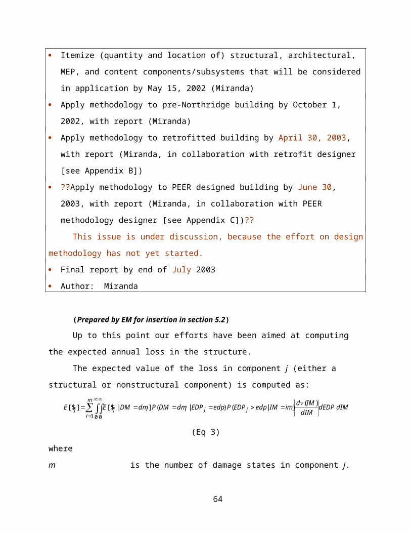
1 2 3 4 5 6 7 9 9

D

C

B

A

RSB1 RSB2 RSB3 RSB3 RSB3 RSB3 RSB2 RSB1

RSB7 RSB3 RSB3 RSB3 RSB2 RSB1RSB9 RSB8

RSB4

RSB6

RSB5

2FSB

14

RSB1

1

2FSB

13

RSB15

RSB12 RB6

RB1

RB2

RB3

RB5

RB4

1 2 3 4 5 6 7 9 9

D

C

B

A

2FSB1 2FSB2 2FSB3 2FSB3 2FSB3 2FSB3 2FSB2 2FSB1

2FSB3 2FSB3 2FSB3 2FSB3 2FSB2 2FSB12FSB8 2FSB7

2FSB

42F

SB6

2FSB

5

2FSB

13

2FSB

10

2FSB

12

2FSB9

2FSB11 2FB3

2FB1

2FB2

2FB2

2FB5

2FB42FB8

2FB6 at floor, 2FB7 mid-landing

1 2 3 4 5 6 7 9 9

D

C

B

A

FSB1 FSB2 FSB3 FSB3 FSB3 FSB3 FSB2 FSB1

FSB3 FSB3 FSB3 FSB3 FSB2 FSB1FSB8 FSB7

FSB4

FSB6

FSB5

FSB1

3

FSB1

0

FSB1

2

FSB9

FSB11 FB3

FB1

FB2

FB2

FB5

FB6 at floor, FB7 mid-landing

FB4FB8

3'-59'-104'-23'-5

8'-9

6'-07'-1 5'-88'-8

Roof

Floors 3-7

Floor 2

Fig. 16. Floor beam and floor spandrel beam plans.

64

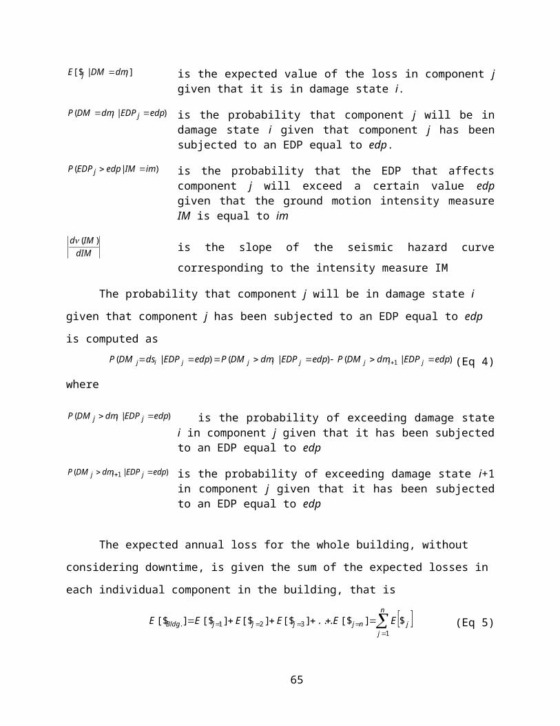
Fig. 17. Arrangement of column steel (Rissman and Rissman Associates, 1965).

Mechanical, electrical, and plumbing plans are no longer available for this building,

either from the City of Los Angeles or the original architect. Equipment conditions were

observed in a walkthough in January, 2002. Through-wall air-conditioning units are mounted in

the waist panels below the windows and provide ventilation to the suites. Central HVAC is

provided only for hallway and ground-floor spaces. Building-service equipment include, on the

ground floor: switchgear and transformers (unanchored, unbraced); anchored hot water heater

and washing machines; and unanchored dryers and water softener. On mechanical pads in the

parking lot: an unanchored transformer and an anchored diesel backup generator. On the roof,

two anchored elevator motors, an anchored upright 1000-gal water tank, anchored cooling tower

(for lobby air conditioning) on steel skids, a kitchen fan on possible unanchored 12-in pipe stilts,

and two packaged air-condition units on two steel skids each supported by two welded 12-in pipe

stilts that do not appear to be anchored to their base. Photos of the equipment are provided on

the CD-ROM included with this report. (During the testbed project, photos can be viewed at

www.peertestbeds.net. They will be permanently archived at PEER.)

Table 7. Column reinforcement schedule.

Column markC13 to

C17, C21 to C26

C11, C12, C20

C30 to C34

C10, C18, C19, C27

C2, C3, C8, C29, C35

C1, C9, C28, C36

C1A, C10A

C17A, C26A

Level Col size 18"x18" 18"x18" 14"x20" 14"x20" 14"x20" 14"x20" 10"x12" 10"x12"7th floor Vert.

bars6-#7 6-#7 6-#7 6-#7 6-#7 6-#7 4-#5

Ties #2@12" #2@12" #2@12" #2@12" #2@12" #2@12" #2@10"6th floor Vert.

bars6-#7 6-#7 6-#7 6-#7 6-#7 6-#7 4-#5 4-#5

Ties #2@12" #2@12" #2@12" #2@12" #2@12" #2@12" #2@10" #2@10"5th floor Vert. 6-#7 6-#8 6-#7 6-#7 6-#7 6-#7 4-#5 4-#5

65

barsTies #2@12" #3@12" #2@12" #2@12" #2@12" #2@12" #2@10" #2@10"

4th floor Vert. bars

6-#8 8-#9 6-#7 6-#9 6-#7 6-#7 4-#5 4-#5

Ties #3@12" #3@12" #2@12" #3@12" #2@12" #2@12" #2@10" #2@10"3rd floor Vert.

bars8-#9 12-#9 6-#9 8-#9 8-#9 6-#7 4-#6 4-#5

Ties #3@12" #3@12" #3@12" #3@12" #3@12" #2@12" #2@10" #2@10"2nd floor Vert.

bars10-#9 12-#9 6-#9 8-#9 8-#9 6-#7 4-#6 4-#5

Ties #3@12" #3@12" #3@12" #3@12" #3@12" #2@12" #2@10" #2@10"1st floor Col size 20"x20" 20"x20"

Vert. bars

10-#9 12-#9 10-#9 12-#9 10-#9 8-#9 4-#8 4-#6

Ties #3@12" #3@12" #3@12" #3@12" #3@12" #3@12" #3@10" #2@10"

Table 8. Spandrel beam reinforcement schedule, floors 3 through 7.

Beam

mark

Width Height Top bars Bottom bars #3 ties

7F 6F 5F 4F 3F

FSB1 16” 22-½” 2#7 2#9 2#9 3#8 3#8 2#7 (2#8 @ 3F, 4F)

3@5”, 5@6”, rest @10”, 3F- 5F

FSB2 top bars 6@4”, 5@6”, 3F-5F

FSB2 16” 22-½” 2#9 3#8 3#8 3#8 3#9 2#6 8@5”, 5@6” ea end

FSB3 top bars Rest @ 10” 3F-5F

FSB3 16” 22-½” 2#8 2#9 3#8 3#8 3#9 2#6 3@5”, 5@6” ea end

Rest @ 10” 3F-5F

FSB7 16” 22-½” FSB3 top bars 2#7 3@5”, 5@6” ea end

FSB8 top bars Rest @ 10” 3F-5F

FSB8 16” 22-½” 2#8 2#9 2#9 3#8 3#8 2#7 (2#8 @ 5F, 2#9 @ 3F, 4F)

3@5”, 5@6”, rest@10” 3F-5F

2#7 2#8 2#9 2#9 3#8 6@4”, 5@6” 3F-5F, , etc.: column lines3F, 4F, etc: floor levels

66

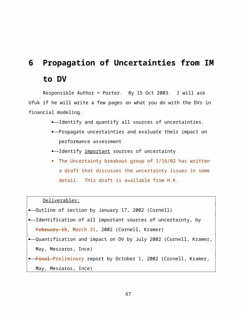
Table 9. Roof and second-floor spandrel beam reinforcement schedule.

Beam mark Width Height Top bars Bottom bars

#3 ties

RSB1 16” 22” 2#6 2#8

2#7 #3@10”

RSB2 16” 22” RSB1 top bars RSB3 top bars

2#6 Same

RSB3 16” 22” 2#8 2#6 Same

RSB7 16” 22” RSB3 top bars 2#9

2#6 Same

RSB8 16” 22” 2#9 3#9

2#9 Same

2FSB1 16” 30” 2#9 2FSB2 top bars

2#8 4 @ 6”, 2 @ 8”, ea end, rest @ 13”

2FSB2 16” 30” 3#8 2FSB3 top bars

2#6 Same

2FSB3 16” 30” 2#9 2#6 Same

2FSB7 16” 30” 2FSB3 top bars 2FSB8 top bars

2#7 Same

2FSB8 16” 30” 2#9 2#9

2#8 Same

A.3 Past Earthquake Damage

Deliverables:

Architectural, mechanical, and structural drawings, soil report, reports on meetings with

owner, architect/engineer (on website, downloadable, as becoming available, to be completed

by March 2002.)

Draft of chapter by April 15, 2002

Final chapter by October 1, 2002

67

The building was strongly shaken by the M6.6 1971 San Fernando event, approximately

20 km to the northeast (Fig. 18). Earth Sciences AR-240 strong-motion accelerometers were

located at the southeast corner of the ground floor, middle of the 4th floor, and southwest corner

of the roof (Fig. 19). The instruments recorded peak accelerations at the ground floor of 240

cm/sec2 in the transverse direction, 130 cm/sec2 longitudinally, an4 170 cm/sec2 in the vertical

direction. Peak roof accelerations were 384 cm/sec2 transverse and 315 cm/sec2 longitudinally at

the southwest corner of the building (Trifunac et al., 1999). The 5%-damped acceleration

response spectra for the ground-floor instruments are shown in Fig. 20 (calculated using Bispec

[Hachem, 2000]).

Islam (1996) reports building periods of 0.70 sec in the early part of the 1971 earthquake,

and 1.5 sec during peak response (Table 10). Hart and Vasdevan (1975) performed system

identification analysis of the accelerometer records to estimate equivalent viscous damping ratios

of 16.4% of critical in the longitudinal direction, 9.7% transverse. McVerry (1979) estimated

17.3% in the longitudinal direction, 19.2% transversely.

Fig. 18. Testbed building (star) relative to 1971 and 1994 earthquakes (EERI, 1994).

68

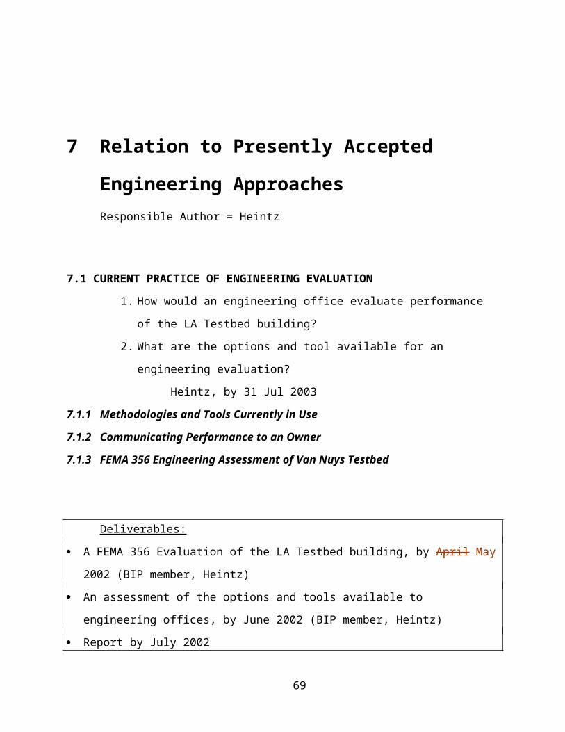
4

6

5

1

3

2

7

9

8

N

1

2

3

4

5

6

7

R

Fig. 19. Instrument locations in 1971 San Fernando earthquake.

0.00

0.25

0.50

0.75

1.00

0.0 0.5 1.0 1.5 2.0 2.5

Period, sec

Spec

tral a

ccel

erat

ion,

g

0.00

0.25

0.50

0.75

1.00

0.0 0.5 1.0 1.5 2.0 2.5

Period, sec

Spec

tral a

ccel

erat

ion,

g

Fig. 20. Spectral acceleration, 1971 ground-floor motions, longit. (left) and transverse (right).

Table 10. Approximate fundamental building periods (Islam, 1996)

69

Longitudinal Transverse Torsional

Pre-1971 San Fernando, ambient vibration 0.52 sec 0.40 sec

1971 San Fernando earthquake

Early part of earthquake 0.70 0.70

During peak response 1.5 1.6

1994 Northridge earthquake

Early part (0-10 sec) 1.5 2.2 1.4

Middle part (10-20 sec) 2.1 2.2

Toward the end (>25 sec) 2.4 2.0

The damage in 1971 mostly required architectural repairs. Jennings (1971) describes

“extensive damage to the interior plaster walls, to the plumbing fixtures, etc., on the second,

third, and fourth floors. The upper three floors were not damaged severely…. The structural

frame received some cracks, indicating strains beyond the elastic limit; the cracks were repaired

with epoxy cement.” John A. Blume & Associates (1973) report:

The structural repair consisted of patching the second-floor beam-column joint on the north side (east end) of the structure…. Some structural distress appeared at some column pour joints located near the exterior beam soffits.… Epoxy repaired the spalled concrete [sic]. Paint was applied to areas where only flaking of paint occurred.

Nonstructural damage was extensive. Almost every guest room suffered some damage. About 80 percent of the repair cost was spent on drywall partitions, bathroom tile, and plumbing fixtures. The damage was most severe on the second and third floors and least severe at the sixth and seventh floors.

Some gypsum wallboard had to be replaced. Interior partitions required paint and new vinyl wall covering…. Forty-five bathtubs … and 12 water closets had to be replaced. Bathroom tile had to be patched, grouted, or replaced in over half the bathrooms…. Spalling occurred at architectural concrete attached to structural concrete columns at the ground floor…. Exterior cement plaster spalled and cracked. Windows in every room required some alighment and caulking, although none needed replacing. Doors needed adjustment.

John A. Blume & Associates (1973) report the repair cost as “approximately $145,000,”

of which $2,000 was for structural repair. Trifunac et al. (1999) report the cost of repair as

$143,000, while Jennings (1971) estimated repair costs as approximately $250,000.

70

In 1980, additional accelerometers were installed; their locations are shown in Fig. 21

(California Strong Motion Instrumentation Program, 2001). As of this writing, they have been

triggered in 11 subsequent events, whose magnitudes, epicentral distances, intensities are shown

in Table 11. According to the available literature, and judging by construction permits on file in

the Los Angeles Department of Building and Safety, none of these subsequent events other than

Northridge series caused significant damage.

Fig. 21. Instrument locations after 1980.

71

Table 11. Events causing strong motion (Trifunac et al., 1999; CSMIP, 1994)

Earthquake Date M R (km)

PGA (cm/sec2) PGV (cm/sec) PGD (cm)Trans Long Trans Long Trans Long

1. San Fernando 9 Feb 1971 6.6 22 240 130 27 23 5.3 9.7

2. Whittier 1 Oct 1987 5.9 41 160 8.7 1.8

3. Whittier aft. 4 Oct 1987 5.3 38 37 52 1.4 2.2 0.3 0.3

4. Pasadena 3 Oct 1988 4.9 32 54 36 1.6 0.9 0.3 0.2

5. Malibu 19 Jan 1989 5.0 36 15 22 0.9 1.0 0.2 0.2

6. Montebello 12 Jun 1989 4.1 34 21 22 0.8 0.8 0.2 0.2

7. Sierra Madre 28 Jun 1991 5.8 44 56 62 4.6 2.8 1.0

8. Landers 28 Jun 1992 7.5 190 41 41 12 11 6.1 4.9

9. Big Bear 28 Jun 1992 6.5 150 25 23 3.6 3.6 0.9 1.0

10. Northridge 17 Jan 1994 6.7 7.2 390 440 40 51 12 7.9

11. Northridge aft. 20 Mar 1994 5.2 1.2 270 140 7.5 4.8 0.6 0.6

12. Northridge aft. 6 Dec 1994 4.5 11 57 60 3.0 2.4 0.5 0.2

Shaking, structural response, and damage in the 1994 Northridge earthquake were more

severe than in the San Fernando earthquake. As noted in Table 11, peak acceleration at the

ground floor was 440 cm/sec2 in the longitudinal direction, 390 cm/sec2 transversely. The 5%-

damped acceleration response spectra for the motion recorded by instruments 16 and 14 are

shown in Fig. 22 (calculated using Bispec [Hachem, 2000]). Assuming a fundamental period of

1.5 to 2.0 sec and 5% viscous damping, the building experienced damped elastic spectral

acceleration of approximately 0.3 to 0.5g.

72

0.0

0.5

1.0

1.5

2.0

0.0 0.5 1.0 1.5 2.0 2.5

Period, sec

Spec

tral a

ccel

erat

ion,

g

0.0

0.5

1.0

1.5

2.0

0.0 0.5 1.0 1.5 2.0 2.5

Period, secSp

ectra

l acc

eler

atio

n, g

Fig. 22. Spectral acceleration of ground-floor motions, 1994 longit. (left) and transverse (right).

Islam (1996) reports structural response in the Northridge earthquake in terms of relative

displacements and transient interstory drift ratios, as shown in Table 12. Several authors have

estimated peak responses at the other floors; Table 12 shows estimates by Li and Jirsa (1998) and

Browning et al. (2000). The table shows fair agreement among the estimates: transient drift

ratios reached approximately 2% in the 1st through 4th stories, decreasing to 0.5% toward the 7th

story.

73

Table 12. Recorded peak displacements and story drift ratios.

FloorMax rel.

displacement(Islam, 1996)

Transient drift ratio relative to floor belowRecorded

(Islam, 1996)Calc., Li & Jirsa

(1998)Calc., Browning

et al. (2000)

Longitudinal

Roof 9.2 in. 0.3% 0.5%

7 0.6% 0.7%

6 8.2 0.9% 1.3%

5 1.9% 1.9%

4 1.7% 1.9%

3 3.6 1.9% 1.9% 1.0%

2 1.6 1.0% 1.8% 0.4%

Transverse

R, east 6.9 in.

R, west 9.0

6, east 6.0

3, east 2.9 1.6%

3, west 3.4 1.3%

2, east 1.6 1.1%

2, west 1.9 1.2%

Trifunac et al. (1999) and Trifunac and Hao (2001) present the results of two thorough

damage surveys performed on February 4, 1994, and April 19, 1994. They report extensive

structural damage, in the form of shear failure of columns and beam-column joints in the

perimeter moment frame. The failures include spalling of the cover concrete over longitudinal

bars, buckling of the longitudinal bars and through-cracks up to several inches wide. Damage to

the south frame occurred at six locations on the 5th floor (column lines A-3, 4, 5, 7, 8, and 9) and

one at the 3rd-floor level (column line A-9), as shown in Fig. 23. Damage to the north frame

occurred in the full-height infill masonry walls at the 1st story, and at the base of the short

columns at the 1st story in column lines D-2, D-3, and D-4. Damage to the north frame also

occurred at or within the beam-column joint at 12 other locations at the 2nd through 5th floors, as

74

shown in Fig. 24. The interested reader is referred to Trifunac et al. (1999) and Trifunac and

Hao (2001) for additional detail, including photos of the damag..

Fig. 23. Structural damage in 1994 Northridge earthquake, south frame (Trifunac et al., 1999)

75

Fig. 24. Structural damage in 1994 Northridge earthquake, north frame (Trifunac et al., 1999)

Structural repairs after the 1994 Northridge earthquake involved the addition of

shearwalls at three columns of the south frame (3, 7, and 8) and four columns of the north frame

(3, 5, 7, and 8), and at several interior column lines. Base fixity is provided to the new

shearwalls by the addition of grade beams spanning between pier groups. Fig. 25 shows the

building as it appeared in March 2001. However, consideration of the testbed building after this

seismic strengthening effort is beyond the scope of the present project.

Fig. 25. Shearwalls added to south (left) and north frames (right) after the 1994 Northridge earthquake. (Left: lines A-3, 7 and 8 from near to far. Right: lines D-8, 7, 5, and 3).

A.4 Occupancy

In order to estimate building-related casualties for a selected building, one first needs to

know the number of occupants in the facility. Building occupancy varies significantly with time

76

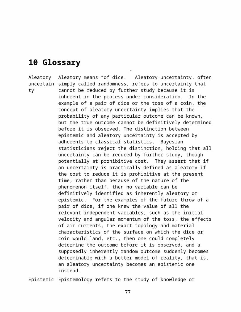
of day and facility use, as well as with building size and configuration. Building occupancy is

typically characterized by general usage (e.g., single family home, office building) at two times

of day; one representing a daytime peak (usually 2 pm) and one representing a nighttime peak

(usually 2 am). The most commonly used published occupancy model is provided by ATC-13:

Earthquake Damage Evaluation Data for California (ATC, 1985). For example, the ATC-13

occupancy model for hotels (ATC social function classification “temporary lodging”) is 0.6

occupants per 1,000 square feet daytime, and 2.5 occupants per 1,000 square feet nighttime2.

The ATC model provides a mean estimate of occupancy by class, with no information regarding

potential variance.

As an alternative to the generalized ATC-13 model, a building-specific occupancy model

can be developed by examining the building layout, and by gathering specific occupancy load

data from the facility manager or occupants. To reflect the uncertainty of the occupancy model,

a building specific model should include, to the extent possible, both a mean occupancy estimate,

as well as a standard deviation or measure of the variance.

In order to estimate fatalities due to collapse of the Van Nuys testbed building, a

building-specific occupancy model was developed from available drawings, and building

information provided by the hotel’s current general manager. The testbed occupancy model

identifies how many people are in the building, as well as where they are located. For

implementation with the PEER Van Nuys testbed fatality model, locations of interest include

those persons on the ground floor (to allow for a reduction in fatalities associated with immediate

escape) and those on upper floors. The temporal distribution is limited to “daytime” and

“nighttime” occupants (approximately 8 am to 8 pm, and 8 pm to 8 am, respectively), along with

peak occupancy levels associated with full hotel occupancy.

There are four classes of occupants within the testbed; hotel guests, hotel staff, restaurant

patrons, and persons attending meetings in the meeting rooms. Data and occupancy rates for

each class of occupants are presented below, with the resulting occupancy model provided in

Table 1.

2 For the 66,150 square foot Van Nuys testbed building, the generalized ATC-13 occupancy model

produces occupancy estimates of 40 daytime occupants and 165 nighttime occupants.

77

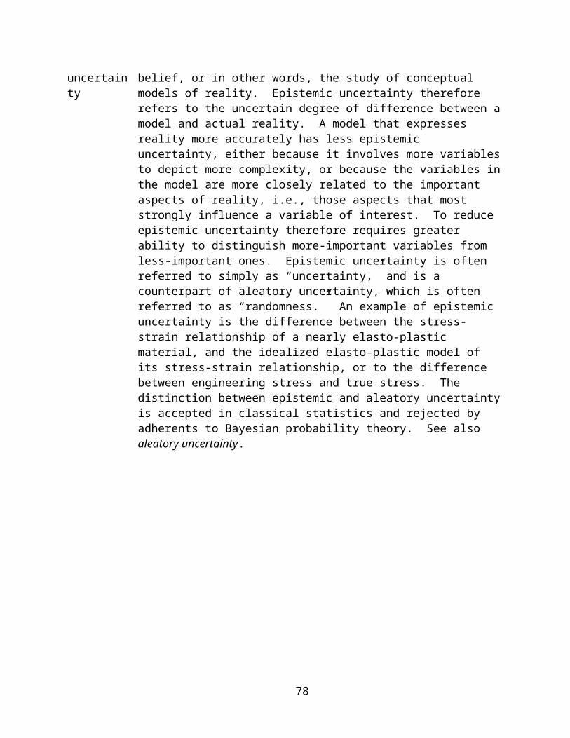
Table 1: Summary of Van Nuys testbed occupancy distribution

Day (approx. 8 am

- 8 pm)

Peak Day (times as noted)

Night (approx. 8 pm

- 8 am)

Peak Night (100%

occupancy)Upper Floors: D-UF PD-UF N-UF PN-UFHotel Guests 20 20 149 198Hotel Staff 9 9 1 2Upper Floors Total 29 29 150 200Ground Floor: D-GF PD-GF N-GF PN-GFHotel Staff 12 26 2 2Restaurant Patrons --- 80 (7:30–8:30am &

11:30am-1:30 pm)134 (5:00–8:00pm)

--- ---

Meeting Attendees 26 200 --- ---Ground Floor Total 38 360 2 2Testbed Total 67 389 152 202

Hotel Guests. The testbed hotel has 132 guest rooms on six floors (22 rooms per floor).

According to the hotel’s general manager (M. Periera, 2003), hotel occupancy rates have

increased slightly since first reported for this project, and now average 75%. The average

number of occupants remains 1.5 persons per room. Further, it is estimated that during the day,

no more than 20 guests are in their rooms at any time.

Accordingly, the typical number of daytime upper floor (D-UF) occupants is 20, while

the typical number of nighttime upper floor occupants (N-UF) is 149. The peak nighttime upper

floor occupancy (PN-UF) is 198 people.

Hotel Staff. According to the hotel’s general manager (M. Periera, 2003), the typical

number of daytime staff is between 20 and 22, with a maximum of 35. At any time during the

day, 7 to 10 hotel staff members are working on the upper floors, with the remainder on the

ground floor. The typical nighttime staffing level is three employees; 2 on the ground floor, and

1 on the upper floors. During peak summer months, one additional nighttime staff person will be

added, covering the upper floors.

The average number of daytime hotel staff on the upper floors (D-UF) is taken to be 9,

while the average number of nighttime upper floor staff (N-UF) is 1. The peak nighttime upper

floor staff (PN-UF) is 2 people. Staffing levels on the ground floor are approximately 12 for

daytime (D-GF) and 2 for nighttime (N-GF). The peak daytime ground floor (PD-GF) staffing

level is taken to be 26.

Restaurant Patrons. The hotel configuration prior to the 1994 Northridge earthquake

included a dining room and a tavern. Occupancy information noted on the architectural first

78

floor plan (Rissman and Rissman Associates, 1965) indicates occupancy loads of 80 for the

restaurant, and 54 for the bar. Peak mealtime occupancies are assumed to be as follows:

1. Breakfast – restaurant at capacity (80) between 7:30 and 8:30 am. (PD-GF=80)

2. Lunch - restaurant at capacity (80) between 11:30 am and 1:30 pm (PD-GF=80)

3. Dinner – restaurant and bar at capacity (134) between 5:00 am and 8:00 pm (PD-GF=134)

Meeting Attendees. Prior to the Northridge earthquake, the Van Nuys testbed hotel had

one large banquet room, which could be subdivided for smaller meetings. Occupancy

information noted on the architectural first floor plan (Rissman and Rissman Associates, 1965)

indicates occupancy loads of 200 in assembly configuration, 94 in dinner configuration.

It appears that the original banquet room is the equivalent of the current “Orion” and

“Van Nuys” meeting rooms combined. (The current “Board Room” meeting room was not part

of the original configuration). These two rooms each measure 19 ft x 36 ft in size, and can each

hold as many as 100 people when set up for a reception, or as few as 40 people in classroom

configuration.

According to the hotel’s General Manager [M. Periera, 2003], the meeting rooms are

typically used three days per week, between the hours of 8am and 5 pm (9 hours), and generally

average 40 occupants for each of the large rooms. This yields an equivalent daytime (12-hour)

occupancy of approximately 26 people (80 people x (9 hrs / 12 hours) x (3 days/7 days)) = 25.71

people, or D-GF = 26). Maximum daytime occupancy (PD-GF) can be taken as 200, assuming

full occupancy.

A.5 References

Applied Technology Council (ATC), 1985, ATC-13, Earthquake Damage Evaluation Data for California, Redwood City, California.

Browning, J., Y.R. Li, A. Lynn, and J.P. Moehle, 2000, “Performance Assessment for a Reinforced Concrete Frame Building,” Earthquake Spectra 16 (3), August 2000, Earthquake Engineering Research Institute, Oakland, CA, 541-556

California Strong Motion Instrumentation Program, 2001, Van Nuys 7-Story Hotel, CSMIP Station No. 24386, California Division of Mines and Geology, Sacramento, CA, ftp://ftp.consrv.ca.gov/pub/dmg/csmip/BuildingPages/BLD24386.HTM

79

City of Los Angeles Dept of Building and Safety, 1966, Application for Inspection of New Building and for Certificate of Occupancy, for 8244 Orion Ave., Sepulveda, Los Angeles, CA

Epstein, H.L., 1965, Holiday Inn of America, Orion Ave, Van Nuys, CA, Structural Calculations, Los Angeles, CA, 183 pp.

Hachem, M.M., 2000, Bispec Ver 1.1.2, University of California, Berkeley, http://www.ce.berkeley.edu/~hachem/bispec.html

Islam, M.S., 1996a, “Analysis of the Response of an Instrumented 7-story Nonductile Concrete Frame Building Damaged During the Northridge Earthquake,” Proceedings of the 1996 Annual Meeting of the Los Angeles Tall Buildings Structural Council, May 10, 1996, Los Angeles, CA.

Islam, M.S., 1996b, “Holiday Inn,” 1994 Northridge Earthquake Buildings Case Study Project Proposition 122: Product 3.2, Sacramento CA: Seismic Safety Commission, 189-233.

Islam, M.S., Gupta, M., and Kunnath, B., 1998, “Critical Review of The State-Of-The-Art Analytical Tools and Acceptance Criterion in Light of Observed Response of an Instrumented Nonductile Concrete Frame Building,” Proceedings, Sixth US National Conference on Earthquake Engineering, Seattle, Washington, May 31-June 4, 1998, Oakland CA: Earthquake Engineering Research Institute, 11 pp.

Jennings, P.C., 1971, Engineering Features of the San Fernando Earthquake of February 9, 1971, Report EERL 71 – 02, Pasadena, CA: California Institute of Technology

John A. Blume & Associates, 1973, “Holiday Inn (29)” San Fernando, California, Earthquake of February 9, 1971, vol. 1, part a, National Oceanographic and Aviation Administration, Washington, DC, 359-393

Li, Y.R., and Jirsa, J.O., 1998, “Nonlinear Analyses of an Instrumented Structure Damaged in the 1994 Northridge Earthquake,” Earthquake Spectra, 14 (2), Earthquake Engineering Research Institute, Oakland, CA, 245-264.

Periera, Martin, personal communication, June 20, 2003.Rissman and Rissman Associates, 1965, Holiday Inn Van Nuys Structural Drawings,

Pacific Palisades, CA

80

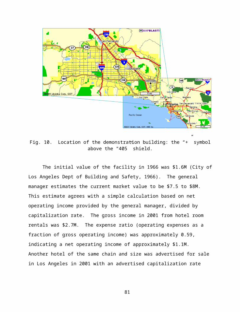
RS Means Co., Inc., 2001, Means Square Foot Assemblies Cost Data 2001, Kingston, MA, 146-147

Scholl, R.E., 1981, Seismic Damage Assessment for Highrise Buildings, Annual Technical Report, Open-file Report 81-381, Menlo Park, CA: US Geological Survey, 143 pp.

Trifunac, M.D., and Hao, T.Y., 2001, 7-Storey Reinforced Concrete Building in Van Nuys, California: Photographs of the Damage from the 1994 Northridge Earthquake, Report CE 01-05, University of Southern California Department of Civil Engineering, Los Angeles, CA, 91 pp, http://www.usc.edu/dept/civil_eng/Earthquake_eng/CE_Reports/01_05/01_05_ALL.PDF

Trifunac, M.D., S.S. Ivanovic, and M.I. Todorovska, 1999, Instrumented 7-Storey Reinforced Concrete Building in Van Nuys, California: Description of the Damage from the 1994 Northridge Earthquake and Strong Motion Data, Report CE 99-02, University of Southern California Department of Civil Engineering, Los Angeles, CA

81

Appendix B. Retrofit DesignDesign of Cost-Effective Retrofit Options (**not yet funded**)

This will be shelved until Year 6, but should get preferential treatment as soon as

funding is available

Krawinkler to outline a work statement by March 1, 2002

82

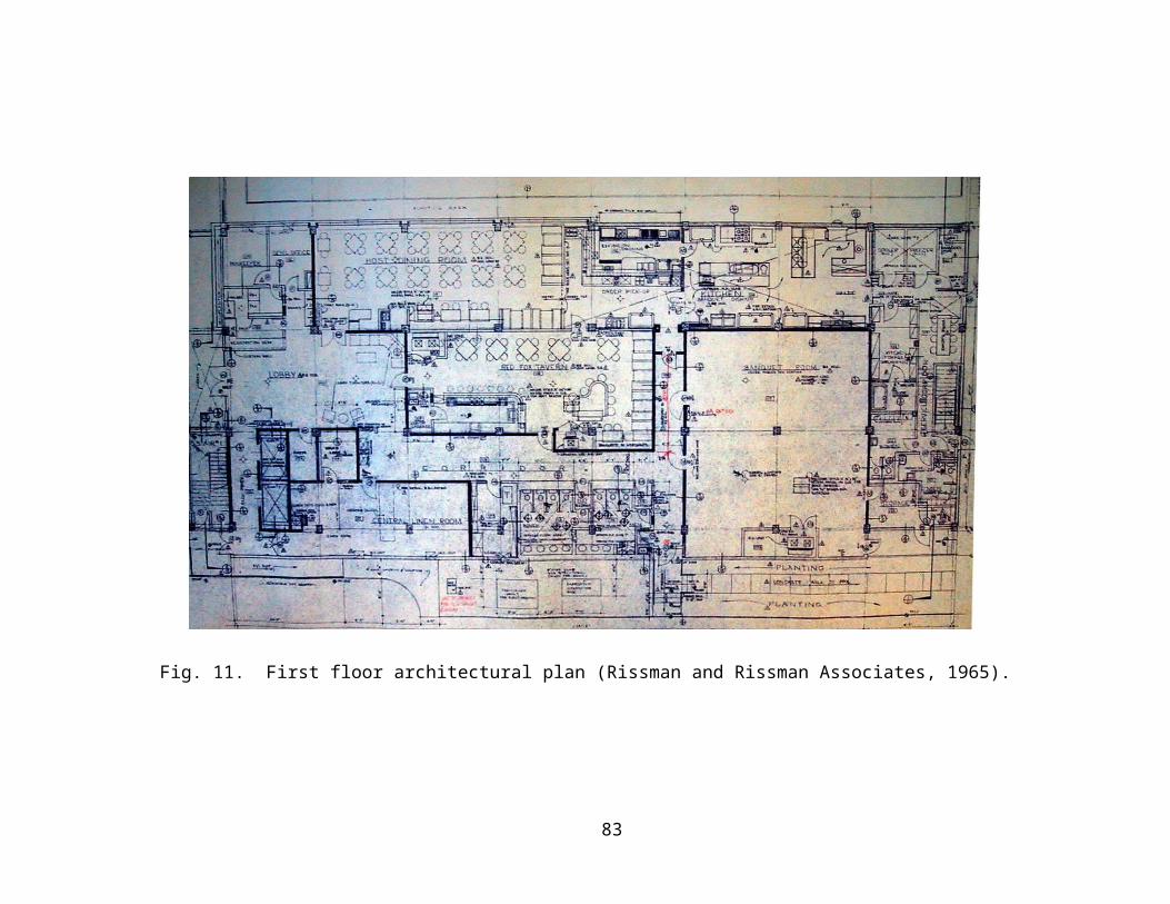
Appendix C. Design By PEER MethodologyDesign Based on PEER PBEE Methodology (**not yet funded**)

This will be shelved until Year 6 (or later).

83