Pentagram Spirals

Richard Evan Schwartz ∗

July 19, 2013

1 Introduction

The pentagram map is a projectively natural map defined on the space of n-gons. The case n = 5 is classical; it goes back at least to Clebsch in the 19thcentury and perhaps even to Gauss. Motzkin [Mot] also considered this casein 1945. I introduced the general version of the pentagram map in 1991. See[Sch1]. I subsequently published two additional papers, [Sch1] and [Sch2],on the topic. Now there is a growing literature. See the discussion below.

To define the pentagram map, one starts with a polygon P and producesa new polygon T (P ), as shown at left in Figure 1.1 for a convex hexagon. Asindicated at right, the map P → T 2(P ) acts naturally on labeled polygons.

P

T(P)2T (P)

P

Figure 1.1: The pentagram map

∗Supported by N.S.F. grant DMS-0604426

1

The pentagram map is defined on polygons over any field. More generally,as I will discuss below, the pentagram map is defined on the so-called twistedpolygons. The pentagram map commutes with projective transformationsand thereby induces a map on spaces of projective equivalence classes ofpolygons, both ordinary and twisted.

The purpose of this paper is to introduce a variant of the pentagrammap, which I will call pentagram spirals . The pentagram spirals relate to thepentagram map much in the way that logarithmic spirals relate to circles. Ihad the idea for pentagram spirals many years ago, but since there was notmuch interest in the pentagram map, I decided not to pursue the idea.

Figure 1.2: The inward half of a pentagram spiral of type (4, 3).

2

In recent years, the pentagram map has attracted a lot of attention,thanks to the following developments.

1. In [Sch3], I found a hierarchy of integrals to the pentagram map, sim-ilar to the KdV hierarchy. I also related the pentagram map to theoctahedral recurrence, and observed that the continuous limit of thepentagram map is the classical Boussinesq equation.

2. In [OST1], Ovsienko, Tabachnikov and I showed that the pentagrammap is a completely integrable system when defined on the space ofprojective classes of twisted polygons. We also elaborated on the con-nection to the Boussinesq equation.

3. In [Sol] Soloviev showed that the pentagram map is completely inte-grable, in the algebro-geometric sense, on spaces of projective classesof real polygons and on spaces of projective classes of complex poly-gons. In particular Soloviev showed that the pentagram map has a Laxpair and he deduced the invariant Poisson structure from the Phong-Krichever universal formula.

4. In [OST2] (independently, at roughly the same time as [Sol]) Ovsienko,Tabachnikov and I showed that the pentagram map is a discrete, com-pletely integrable system, in the sense of Liouville-Arnold, when definedon the space of projective classes of closed convex polygons.

5. In [Gli1], Glick identified the pentagram map with a specific clusteralgebra, and found algebraic formulas for iterates of the map whichare similar in spirit to those found by Robbins and Rumsey for theoctahedral recurrence.

6. In [GSTV], Gekhtman, Shapiro, Tabachnikov, Vainshtein generalizedthe pentagram map to similar maps using longer diagonals, and definedon spaces of so-called corrugated polygons in higher dimensions. Thework in [GSTV] generalizes Glick’s cluster algebra.

7. In [MB1], Mari-Beffa defines higher dimensional generalizations of thepentagram map and relates their continuous limits to various familiesof integrable PDEs. See also [MB2].

3

8. In the recent [KS], Khesin and Soloviev obtain definitive results abouthigher dimensional analogues of the pentagram map, their integrability,and their connection to KdV-type equations.

9. In the preprint [FM], Fock and Marshakov relate the pentagram mapto, among other things, Poisson Lie groups.

10. The preprint [KDiF] discusses many aspects of the octahedral recur-rence, drawing connections to the work in [GSTV].

Though this is not directly related to the pentagram map, it seems alsoworth mentioning the recent paper [GK] of Goncharov and Kenyon, whostudy a family of cluster integrable systems. These systems are closely re-lated to the octahedral recurrence which, in turn, is closely related to thepentagram map.

Informally, a pentagram spiral is a bi-infinite polygonal path P in theprojective plane such that some finite power of the pentagram map carriesP to itself when P is considered as an unlabeled path. §3.1 has a formaldefinition. The global combinatorics of how this is done allows one to describethe type of the spiral by a pair of integers (n, k). For instance, k is the smallestinteger such that T k(P ) = P , as an unlabeled path. The combinatorics ofthe situation will be discussed in §3.2.

For every pair (n, k) with n ≥ 4 and k = 1, ..., (n− 1), I will introduce apentagram spiral of type (n, k). I will focus on the case when the spirals arewhat I call properly locally convex , or PLC for short. The example in Figure1.2 is PLC. Though it is not nearly as obvious as in the case of polygons,the basic constructions which generate the polygon spirals just depend ondrawing and intersecting lines in the projective plane. Thus, they makesense over essentially any field. However, we shall be interested mainly inthe PLC case.

We label the vertices of the spiral by consecutive integers, so that theintegers increase as the spiral moves inwards. A labeled pentagram spiral isreally just the same thing as a pentagram spiral with a distingished vertex.In §3 we will prove

Theorem 1.1 The space C(n, k) of projective equivalence classes of labeled

PLC pentagram spirals of type (n, k) has dimension (2n − 8) + k and is

diffeomorphic to an open ball.

4

This result really amounts to describing how one generates pictures likeFigure 1.2. The space C(n, k) should be seen as a relative of the space C(n)of projective classes of closed convex n-gons. The space C(n) has dimension2n− 8 and is diffeomorphic to an open ball.

The spaces C(n, k) are naturally shift spaces , in that there is a naturalmap

Tn,k : C(n, k) → C(n, k) (1)

which just amounts to moving the distinguished vertex inwards. During thecourse of our proof of Theorem 1.1, we will define Tn,k from several points ofview.

When properly interpreted, the map Tn,k is a dth root of the pentagrammap, where d = 2k/(2n + k). At the same time, when n is large and k issmall, the space C(n, k) is an approximation of the space C(n). Thus, Tn,k

in these cases is a very high root of a map which is close to the pentagrammap. Independent of the intrinsic beauty of the pentagram spirals, it seemsuseful to have these high roots of approximations to the pentagram map.

In §4 we will introduce projectively natural coordinates on the spaceC(n, k) and exhibit a Tn,k invarant function. This is the analog of the in-variant function used in [Sch1] and [Sch2]. For experts, our first invariantfunction is the analogue of what is, in the closed case, one of the Casimirsfor the invariant Poisson structure.

In §5 we will prove the following compactness result, which is similar inspirit to a similar result in [Sch1].

Theorem 1.2 The orbits of Tn,k have compact closure in C(n, k).

Theorem 1.2 says that up to projective equivalence one sees roughly thesame shape, over and over again, as one moves inwards or outwards alongthe spirals. The proof just involves showing that our invariant function hascompact level sets.

In §6 we will use Theorem 1.2 to deduce several geometric corollariesabout PLC pentagram spirals.

Theorem 1.3 The ω-limit set of a PLC pentagram spiral, in the projective

plane, is a union of a single point and a single line. Equivalently, the support

of the triangulation associated to a pentagram spiral is projectively equivalent

to a punctured Euclidean plane.

5

Theorem 1.3 implies that the forward direction of P spirals down to asingle limit point . One might wonder about the nature of this spiraling.

Theorem 1.4 A PLC pentagram spiral winds infinitely many times around

its limit point.

Theorems 1.3 and 1.4 pin down some of the rough geometry of the tri-angulations associated to the pentagram spirals. Theorem 1.3 is the analogof the result in [Sch1] which says that the pentagram map shrinks arbitraryconvex polygons to single points. The triangulations associated to the pen-tagram spirals are locally the same as the triangulations one sees when onetakes the full orbit of a convex polygon under the pentagram map. However,the global structure of the tilings is different.

The main purpose of this paper is geometric. The above results answerprobably the most basic geometric questions one would want to know aboutPLC pentagram spirals. I believe that the deep algebraic structure underly-ing the pentagram map is also present in the pentagram spirals, and I hopethat this paper imspires future work on these objects. In the informal §7, Iwill discuss some computer experiments, conjectures, and topics for furtherstudy.

I wrote a Java program which allows the user to draw the pentagramspirals for smallish values of n and k, and also to watch the spirals evolveunder the map Tn,k. You can download this program at

http://www.math.brown.edu/∼res/Java/SPIRAL.tar

I strongly suggest that the reader interested in this paper download theprogram and play with it. I think that the program greatly enriches thepaper.

This paper contains rigorous proofs of all the main results, but it seemsworth mentioning that I checked the results numerically using my computerprogram. For instance, my program draws the pentagram spirals using ex-actly the formula for Tn,k given in §3.4. The program also lets the user seethat the invariant function Z defined in §4.4 is indeed an invariant of themap Tn,k.

I first thought about the pentagram spirals many years ago when I wastalking to Peter Doyle about his so-called Doyle spirals. The Doyle spiralsare circle packings which relate to the hexagonal circle packing much in the

6

way that the pentagram spirals relate to the pentagram map. Recently Iwalked through the streets of Nice on a pleasant spring night and thoughtback to the puzzles of my youth. In a nostalgic mood, I decided to send ashort note about the pentagram spirals to some of the researchers interestedin the pentagram map. After sending the note, I got the bug again anddecided to write a more systematic paper about them.

I’d like to thank Valentin Ovsienko and Sergei Tabachnikov, my usual col-laborators on the pentagram map, for many discussions about the pentagrammap and related areas of mathematics. This work was carried out during mysabbatical at Oxford in 2012-13. I would especially like to thank All SoulsCollege, Oxford, for providing a wonderful research environment. My sab-batical was funded from many sources. I would like to thank the NationalScience Foundation, All Souls College, the Oxford Maths Institute, the Si-mons Foundation, the Leverhulme Trust, the Chancellor’s Professorship, andBrown University for their support during this time period.

7

2 Preliminaries

2.1 Projective Geometry

The real projective plane RP2 is the space of lines through the origin in R

3.Such lines are denoted by [x : y : z]. This is the line consisting of all vectorsof the form (rx, ry, rz) with r ∈ R.

In the usual way, we think of R2 as an affine patch of RP2. Concretely,

the inclusion is given by(x, y) → [x : y : 1]. (2)

A line in RP2 is a collection of points represented by all the lines in a

plane through the origin in R3. The set RP

2−R2 is a single line, called the

line at infinity . All other lines in RP2 intersect R2 in a straight line. Con-

versely, any straight line construction in R2 extends naturally to a straight

line construction in RP2. When we make our constructions, we will draw

things in the plane (of course) but we really mean to make the constructionsin the projective plane.

A projective transformation is a self-homeomorphism of RP2 induced by

the action of an invertible linear transformation. Projective transformationspermute the lines of RP

2 and are in fact analytic diffeomorphisms. Con-versely any homeomorphism ofRP

2 which carries lines to lines is a projectivetransformation.

A projective construction is one in which points and lines are producedby the following two operations:

• Given distinct points a and b, take the line (ab) through a and b.

• Given distinct lines l and m, take the intersection l ∩m.

We use the notation (ab)(cd) to denote the intersection of the line (ab) withthe line (cd). Since projective transformations carry lines to lines, any pro-jective construction commutes with the action of the group of projectivetransformations.

A subset ofRP2 is convex if some image of that subset under a projective

transformation is a convex subset of R2 in the ordinary sense. For instance,a hyperbola in the plane extends to a closed loop in RP

2 which bounds aconvex subset on one side. Proof: one can move the hyperbola by a projectivetransformation so that it is a circle in the plane.

8

2.2 The Cross Ratio

The inverse cross ratio of 4 real numbers a, b, c, d ∈ R is the quantity

[a, b, c, d] =(a− b)(c− d)

(a− c)(b− d)(3)

When a < b < c < d, the quantity [a, b, c, d] lies in (0, 1). We will usuallyconsider this situation.

Given 4 collinear points A,B,C,D in the projective plane, we choosesome projective transformation which identifies these points with 4 numberson the x-axis, and then we take the cross ratio of the first coordinates ofthese numbers. This lets us define [A,B,C,D]. The result is independent ofany choices made. In particular

[A,B,C,D] = [T (A), T (B), T (C), T (D)] (4)

for any projective transformation T .

2.3 The Corner Invariants

In [Sch3] I introduced the notion of corner invariants of a polygon in theprojective plane. We also used these invariants in [OST1] and [OST2]. Forthe basic definition we will follow the notation in [OST2], but then we willrevert back to an interpretation of the invariants given in [Sch3].

The corner invariants of a polygonal path P with successive vertices {vi}are defined as follows.

We definex3 = [v0, v1, (v0v1)(v2v3), (v0v1)(v3v4)] (5)

x4 = [v4, v3, (v4v3)(v2v1), (v4v3)(v1v0)]. (6)

The remaining invariants are defined by shifting the indices by 2k fork ∈ Z. Figure 2.1 shows a picture of the construction.

9

0

43

2

1

(43)(21)

(01)(34)

(01)(23)

Figure 2.1: The corner invariants

When the curve is such that every 5 consecutive points make the verticesof a convex pentagon, the invariants all lie in (0, 1).

The corner invariants are projectively natural. They provide projectivelynatural coordinates on the space of polygons. Two polygons are projectiveequivalent if and only if they have the same corner invariants. See [Sch3] fordetails. We can express the pentagram map in these coordinates, providedthat we “break symmetry” and choose a less than canonical labeling schemefor P and T (P ). We label the vertices of P ′ = T (P ) so that

v′1 = (v0v2)(v1v3). (7)

The remaining labels are obtained by shifting the indices. In [OST2], wecalled this the right convention. Using the right convention, we have

x′

2 = x4

1− x5x6

1− x1x2

, x′

3 = x3

1− x1x2

1− x5x6

. (8)

The remaining equations are obtained by shifting the indices by 2k. Theseequations are less than perfectly symmetric, on account of the symmetry-breaking labeling convention. However, they served our purposes in [OST1]and [OST2]. In the next section we will explain a more symmetric picture.

10

2.4 Tiling Interpretation of the Coordinates

For convenience we work with bi-infinite paths. Before getting to the paths,however, we will dicsuss a seemingly different construction. We considera hexagonal tiling of the plane, by right-angled isosceles triangles whosehypotenuse is horizontal. Figure 2.2 shows a small part of this triangulation.

G

AB

D

C

E F

Figure 2.2: The corner invariants

We label the edges of the triangulation by real numbers and we insist onthe compatibility relations

AB = CD, G = 1− EF. (9)

These relations are meant to hold for the labels of all the isometric images ofthese configurations. The configurations may be translated or reflected. Wecall such a labeling a pentagram labeling .

If we label the diagonal edges of one row of diagonals, we can fill in theremaining labels using the compatibility rules. This will certainly remindsome readers of the octahedral recurrence, and indeed we worked out theconnection explicitly in [Sch3].

To see the connection between the pentagram labelings and the penta-gram map, we fill in two rows of diagonal edges with the corner invariants,as in Figure 2.3.

11

y5

x1

1−x1x2 1−x3x4 1−x5x6

x3x2 x4 x5 x6

y1 y2 y3 y4

Figure 2.3: The pentagram map seen on the tiling

For ease of labeling we set yi = x′

i. The compatibility rules above expressthe y-coordinates in terms of the x-coordinates, and the formula is exactly asgiven for the pentagram map in Equation 8. The cost of breaking symmetryis that the correspondence between the triangulation labels with the cornerinvariants is somewhat asymmetric. Indeed, if we wanted to continue thiscorrespondence down to the next row of the tiling, so to speak, we wouldhave to switch from the right to the left labeling convention.

In [Sch3] we used a different scheme, whereby the corner invariants cor-responded not to vertices of the polygon but rather flags. The system in[Sch3] worked perfectly from the point of view of lining up the pentagrampicture with the tiling picture, but the apparatus was somewhat cumber-some. Ultimately, we dropped this scheme in [OST1] and [OST2], settlingon something less canonical but more businesslike. In §4 we will try for thebest of both worlds, choosing a convention for the corner invariants whichcaptures the symmetry in [Sch3] but retains the efficient nature of [OST1]and [OST2]

In case we are working in C(n), the labelings we get are periodic withrespect to a horizontal translation by n. (We think of the horizontal edgesas having unit length.) In this case, the reader can probably see that theproducts

E(P ) =n∏

i=1

x2i, O(P ) =n∏

i=1

x2i+1 (10)

are such that

E(T (P )) = O(P ), O(T (P )) = E(P ). (11)

Thus E and O are invariants of the square of the pentagram map. These arethe first invariants of many.

12

3 The Space of Pentagram Spirals

3.1 Basic Definitions

It is actually not so easy to give a formal definition of a pentagram spiral.We will start out with an easy provisional definition but then we will ex-plain the problems with it. Our final definition is somewhat more technical.In the discussion, T denotes the pentagram map, defined on unlabeled paths.

Definition: A bi-infinite polygonal path P ⊂ RP2 is a weak pentagram

spiral if path P ⊂ RP2 with the following there is some integer k > 0 such

that T k is defined on P and T k(P ) = P . The smallest k with this propertyis called the order of P .

It is important to note that perhaps T k(P ) = P only in the unlabeled sense.For instance, when k is even, there is a canonical notion of an action of T onlabeled bi-infinite paths. In this situation, it might be the case that T k(P )and P do not agree as labeled paths.

The definition above is too broad to be of use to us. For example, supposewe have a polygonQ which is periodic under the pentagram map, in the literalsense that T k(Q) = Q. The pentagram map has many periodic points whenacting on projective classes of polygons, but here we mean that the actualpolygon is periodic with respect to the pentagram map. We do not have anexplicit example of this, but presumably it can happen in the non-convexcase. Then we could take P to be a bi-infinite path which winds around Qinfinitely often in both directions. The path Q would be a weak pentagramspiral according to the definition above.

Here is the definition we care about.

Definition: A propertly locally convex pentagram spiral is a weak penta-gram spiral P of order k such that the iterates T j(P ) are embedded, locallyconvex, and pairwise disjoint, for j = 0, ..., (k − 1).

We will usually abbreviate properly locally convex to PLC . Figure 3.1shows an example of a PLC pentagram spiral of order 2. These spirals aremeant to go outwards as well as inwards.

13

Figure 3.1: A PLC pentagram spiral of type (5, 2).

We are not interested in pentagram spirals which are not PLC, but wegive a formal definition for the interested reader. To make this definition gomore smoothly, we will assume Theorem 1.3. Suitably normalized, a PLCpentagram spiral defines a triangulation of the punctured plane. Figure 3.1shows the “inner half” of this triangulation. We call this tiling a PLC tiling.

Let τ denote a PLC tiling. An adapted immersion of τ is continuous mapfrom τ into RP

2 which maps each line segment of τ to a line segment inRP

2. We also require the map to carry each triangle of τ to a nontrivialtriangle.

Definition: A pentagram spiral is the image of a PLC pentagram spiralunder an adapted immersion of the corresponding PLC tiling.

Essentially, a pentagram spiral is an object which has the same locallycombinatorial structure as a PLC pentagram spiral. Since we only discussPLC pentagram spirals in this paper, the reader need not absorb this lastdefinition in order to understand the rest of the paper.

14

3.2 Combinatorics of Pentagram Spirals

We will always work with PLC pentagram spirals, though what we say usuallyworks for a general pentagram spiral. We label the vertices of each pentagramspiral by the integers, so that the numbers increase as one moves inwardsalong the spiral. In our example in Figure 3.1, the map T 2 carries P to itselfbut T 2(Pj) = Pj+6 for all j ∈ Z. Here Pj is the jth point of P . In general,there is some number µ, either a whole or a half integer, such that

T 2k(Pj) = Pj+2µ. (12)

The pair of numbers (µ, k) characterizes the combinatorial type of the tilingproduced by iterating T on the spiral. In Figure 3.1, we have µ = 6. InFigure 1.2, we have µ = 51

2.

We find it more convenient to replace µ with another invariant whichcaptures the same information. We will use the pair (n, k) where k is theorder of the spiral and

n = µ−k

2. (13)

Geometrically, it turns out that n counts the number of sides of the “seed”which generates the spiral. We will explain precisely what we mean by a seedin the next section, but informally, the seed is the outer polygon in Figures1.2 and 3.1. So, we have n = 4 in Figure 1.2 and n = 5 in Figure 3.1.

There is a natural map on the space of pentagram spirals of type (n, k),which we call Tn,k. The map Tn,k shifts the labeling of a spiral by one unit.Thus Tn,k(P ) is the same unlabeled spiral as P , but the kth vertex of Tn,k(P )is the (k+1)st vertex of P . It seems at first that the map Tn,k is trivial, butin fact, on labeled pentagram spirals we have

T 2n+kn,k (P ) = T 2k(P ). (14)

In the next several sections, we will develop the idea of generating a PLCpentagram spiral from a seed. The reason we do this is 2-fold. First, theseeds give a convenient way for drawing the spirals. Second, it turns out thatTn,k can be interpreted as a kind of evolution operator on the set of seeds.The spirals are generated by considering the orbit of the seed under powersof Tn,k.

Once we have the basic constructions involving seeds, we will prove The-orem 1.1. The basic idea is to show that every seed generates a PCL spiraland that every PLC spiral comes from a seed. Finally, we will identify theversion of Tn,k given in terms of seeds with the shift map discussed above.

15

3.3 Seeds

A seed of type (n, k) is a strictly convex n-gon with an additional pointchosen in the interior of each of the last k edges. More precisely, the verticesare points A1, ..., An and the additional Bn−k+1, ..., Bn. Here Bj lies in theinterior of the edge AjAj+1, with indices taken mod n. We will sometimesdenote our seeds as (A,B), where A is short for {A1, ..., An} and B is shortfor {Bn−k+1, ..., Bn}.

5

5

1 2

3

3

4

4

Figure 3.2: A seed of type (5, 3).

Figure 3.2 shows an example of a seed of type (5, 3). The labeling shouldbe fairly obvious: The vertex labeled m denotes Am and the point labeled min the middle of an edge denotes Bm. We decorate the polygon with thicksegments of the following kind:

• (AiAi+1) for i = 1, ..., (n− k + 1).

• (Ai, Bi) for i = (n− k + 1), .., n.

We call these segments the spiral segments . The idea is that a PLC penta-gram spiral and its iterates under the pentagram map will turn out to be aninfinite union of spiral segments, taken from an infinite union of seeds whichpiece together in a way that we explain in the next section.

16

3.4 The Seed Map

Figure 3.3 shows a special case of the general projective construction whichproduces a new seed from an old one.

3

4

5

5

4

4 3 3

2

1

5

5

4

1 2

3

Figure 3.3: One seed produces another.

The boundary of the shaded region is the polygon supporting the newseed. The outside numbers are the old seed labels and the inside numbersare the new seed labels. Putting a star for the new points, we have

• A∗

i = Ai+1 for i = 1, 2.

• Ai = B∗

i for i = 3, 4, 5.

• B∗

5 = (A1A∗

2)(A∗

5A∗

1).

• B∗

i = (Ai+1B∗

i+1)(A∗

iA∗

i+1) for i = 3, 4.

In the last item, we must construct the point with the larger index (i = 5)first. Notice that the spiral segments on the two seeds line up to producewhat promises to be a union of spirals. Figure 3.6 below adds another seed,making the connection to the pentagram map somewhat clearer.

17

4

34

4

1

23

4

3

1 2

34 3

2

4

1

2

3

44

3

2

1 2

3

Figure 3.4: The (4, 2) and (4, 3) cases of the construction.

Figure 3.4 shows two more examples.In general, we define

Tn,k(A1, ..., An;Bn−k+1, ..., Bn) = (A∗

1, ..., A∗

n;B∗

n−k+1, ..., B∗

n) (15)

according to the following rules.

• A∗

i = Ai+1 for i = 1, ..., (n− k).

• A∗

i = Bi for i = (n− k + 1), ..., n.

• B∗

n = (A1A∗

2)(A∗

nA∗

1).

• B∗

j = (Aj+1B∗

j+1)(A∗

jA∗

j+1) for j = (n− 1), ..., (n− k + 1).

In the last item, it is important that the points are constructed going fromthe largest to the smallest index, so that the map is a projective construction.

Lemma 3.1 The starred points form a new seed of the same type.

Proof: The A∗ polygon is obtained from the A polygon by cutting off kcorners using non-overlapping line segments. Hence A∗ is a strictly convexpolygon. The triangle A1A

∗

1A∗

n is nondegenerate and oriented counterclock-wise. A routine induction argument shows that the triangles AjA

∗

jB∗

j arealso nondegenerate and oriented counterclockwise for j = n, ..., (n − k + 2).These facts, together with the definition of the point, imply that each B∗

j liesin the interior of the segment A∗

jA∗

j+1 ♠

18

3.5 The Inverse Map

Figure 3.5, which is a repeat of Figure 3.3 but with different shading, can beinterpreted instead as an illustration of how one can derive outer seed fromthe inner one.

5

5

4

4 3 3

2

1

5

5

4

1 2

3

3

4

Figure 3.5: Figure 3.3 repeated.

We leave it to the reader to check that, in general,

• Ai = A∗

i−1 for i = 2, ..., (n− k + 1).

• Bi = A∗

i for i = (n− k + 1), ..., n.

• Ai = (Ai−1Bi−1)(B∗

i−1B∗

i ) for i = (n− k + 2), ..., n.

• A1 = (AnBn)(A∗

2B∗

n).

This gives us a formula for the inverse map T−1

n,k .

It remains to check that T−1

n,k carries seeds to seeds. If we know in advance

that (A,B) is a seed, then T−1

n,k(A∗, B∗) must be a seed, namely (A,B).

However, what we want to show is that T−1

n,k carries an arbitrary seed to aseed.

19

As readers familiar with the pentagram map know, the inverse of thepentagram map can certainly carry a convex polygon in the plane to a non-convex polygon. However, the inverse of the pentagram map always carries aconvex polygon in the projective plane to a convex polygon in the projectiveplane. The same goes for the the seed map.

Lemma 3.2 If (A∗, B∗) is an arbitrary seed of type (n, k), then the pre-image

(A,B) = T−1

n,k(A∗, B∗) is a seed of the same type.

Proof: First we will show that A is a convex polygon in the projective plane.A is obtained from A∗ by gluing on finitely many shaded triangles, as shownin Figure 3.5. These triangles are constructed successively, starting withA∗

n−k+1A∗

n−k+1An−k+2 and then going counterclockwise. A routine inductiveargument shows that these triangles are never degenerate.

We know that there are some choices of seed (A∗, B∗), namely those in theimage of Tn,k, which give rise to a strictly convex polygon A. We can considera continuous path from a seed which has this property to the seed we areinterested in. The fact that the abovementioned triangles never degenerateimplies that the convexity property is both an open and closed conditionalong our path of A-polygons. Since the initial A-polygon is strictly convex,so is the final one.

It follows from the definition of T−1

n,k that each point Bj lies on the linesegment AjAj+1. Each edge of the form BjAj and BjAj+1 appears as anedge of one of the shaded triangles. Hence these edges are all nontrivial.This forces Bj to lie in the interior of the segment AjAj+1. ♠

Remark: Projective dualities conjugate the pentagram map (suitably inter-preted) to its inverse. The same ought to be true for the map Tn,k, providedthat seeds can be interpreted in a way that puts points and lines on the samefooting. The reader who stares hard enough at Figure 3.5 will eventually seethat this is possible. Given the interaction with duality, the two maps Tn,k

and T−1

n,k are on the same footing and Lemma 3.2 is obvious.

It we interpret C(n, k) as the space of projective classes of seeds of type(n, k), then C(n, k) is clearly a cell of dimension (2n− 8)+k. Indeed, C(n, k)is just a decorated version of C(n). The maps Tn,k and T−1

n,k both acts assmooth diffeomorphisms on C(n, k). To prove Theorem 1.1, it only remainsto reconcile our definition here with the ones made in §3.1.

20

3.6 Reconciling the Two Definitions

In this section we finish the proof of Theorem 1.1 by reconciling the twopoints of view, namely

1. C(n, k) is the space of seeds of type (n, k) and Tn,k is the evolutionoperator defined above by a projective construction.

2. C(n, k) is the space of labeled PLC pentagram spirals of type (n, k) andTn,k is the shift map in this space.

Suppose we start with the first point of view. Let (A,B) be a seed. Theunion of the spiral segments in the bi-infinite orbit

⋃

q∈Z

T qn,k(A,B) (16)

consists of k embedded and locally convex bi-infinite paths in the plane. Tosee that these paths are pentagram spirals, we just have to see that thepentagram map permutes them. This is most easily seen by looking at 3consecutive seeds, as in Figure 3.6.

Figure 3.6: Three consecutive seeds

21

Looking at Figure 3.6 (and generalizing) we see that each line drawn inthe construction of the middle seed is a shortest diagonal of one of the spirals.Since this is true for the middle seed in any sequence of 3 consecutive seeds,this fact is true for every seed in the union in Equation 16. Moreover, thewhite points on each spiral are revealed to be on the image of the “previous”spiral under the pentagram map. Since this is true for the correspondingpoints of the middle seed in every consecutive run of 3 in Equation 16, wesee that the pentagram map indeed permutes the distinghished polygonalpaths. Hence, these paths are all pentagram spirals.

We label our pentagram spirals so that the distinguished point is thepoint A1 of the seed (A,B). We can think of Tn,k as acting on the union inEquation 16. Tn,k takes this union to exactly the same union, except that itis based on the seed (A∗, B∗) = Tn,k(A,B). All that has happened is thatthe new distinguished point is A∗

1, the first point of the new seed. The arrowat the bottom of Figure 3.6 points from A1 to A∗

1. With this interpretation,Tn,k clearly acts as the shift map on our pentagram spirals.

In short, every seed generates a labeled pentagram spiral, and the seedmap acts a shift on the spiral. Thus, for at least some pentagram spirals,namely those generated by seeds, the two points of view coincide. It remainsto see that every pentagram spiral is generated by a seed. We will be a bitsketchy in our argument because we don’t care much about the result. Ifit turned out that there were some exotic pentagram spirals which did notcome from seeds, we would simply add the condition to our definition thatthe spiral come from a seed.

Lemma 3.3 Every pentagram spiral is generated by a seed.

Proof: Let Σ be a pentagram spiral. We interpret Σ as an infinite triangula-tion of some subset of the projective plane. The numbers n and k associatedto Σ characterize the global combinatorics of the tiling. Let Σ′ be a penta-gram spiral produced by a seed of type (n, k). The tiling Σ′ has the samecombinatorics as the tiling Σ. That is, there is a homeomorphism h whichcarries the one triangulation to the other – vertices are taken to vertices andedges are taken to edges. Moreover, certain triples of edges in Σ and in Σ′

line up to form longer line segments – the diagonals used in the pentagrammap. h respects this additional collinearity. Evidently h maps a seed for Σ′

to a seed for Σ. ♠

22

4 Invariant Coordinates

4.1 Flags

We mentioned in §2.4 that we would inprove upon the labeling scheme from§2. The key is to use flags rather than points or lines. On a polygonal path,a flag is a pair (v, e) where v is a vertex of the path and e is an edge of thepath. We indicate the flag (v, e) with an auxilliary point placed on the edgee two-thirds of the way towards v. Figure 4.1 shows what we mean.

e vFigure 4.1: Denoting the flag (v, e).

Suppose we have an oriented polygonal path, as shown in Figure 4.2. Weorient the flags according to the following scheme.

8

3

4

5

6

7

12

Figure 4.2: Ordering the flags along an oriented path

Finally, to each flag along such a path, we associate the cross ratio of theassociated points shown in Figure 4.3. This picture is meant to be invariantunder projective transformations. We call these the flag invariants .

23

Figure 4.3: Invariant of a flag

Let us consider the naturality of this construction. The cross ratio ofinterest can be computed in two ways. First of all, it is the cross ratio ofthe 4 points shown. Two of the points involved are adjacent to the flagpoint. On the other hand, the cross ratio can be computed as the cross ratioof the 4 drawn lines. Two of the lines are adjacent to the line of the flag,going in the other direction from the abovementioned points. Indeed, theentire picture is invariant not just under projective transformations but alsoprojective dualities. Were we to apply a projective duality to the picture,producing another polygonal curve (with points and lines interchanged) theinvariant associated to the flag would be the same. In short, the invariantwe have associated to the given flag is the canonical choice.

Moreover, the ordering of the flags in Figure 4.2 reproduces the orderingof the invariants listed in §2.3. The difference is that, when we work with theflags, there is a canonical way to line up the variables of the path P and itsimage T (P ) under the pentagram map. Figure 4.4 below shows this. Withthis new scheme, there is a natural way to transfer the flag labels to thehexagonal tiling so that the compatibility conditions hold. The method issuch that same-numbered flags correspond to diagonal edges whose centersare on the same vertical. This is illustrates in Figure 4.5. With this newscheme, one need not change labeling conventions at each level.

24

P

T(P)

1

23

3 21

Figure 4.4: Canonical labeling for the pentagram map.

3

1 4

1 4

1 2 4

2

2 3

3

Figure 4.5: Transfer of labels to the tiling.

25

4.2 Pentagram Tilings Revisited

Let T denote the infinite triangular tiling discussed in §2.4. Again, we nor-malize T so that the horizontal edges have length 1. The height of eachtriange is 1/2. Let T denote the set of all pentagram tilings of the edges ofT .

Let T (n, k) denote the set of pentagram tilings which are invariant undertranslation by the vector

V n, k =(n+

k

2,k

2

). (17)

This vector has half-integer coordinates, and the sum of the two coordinatesis an integer. Hence, translation by Vn,k is an isometry of T . Thus, thedefinition of T (n, k) is not vacuous.

Comparing the discussion in §3.1 with the scheme for transfering the flaginvariants of flags to the labels of T , we see that each element of C(n, k)gives rise to a unique element of T (n, k). To make this completely precise,we translate T so that one vertex lies at the origin. We arrange that thediagonal edge joining (0, 0) to (1/2, 1/2) (respectively to (−1/2,−1/2)) cor-responds to the flag just inward (respectively outward) from the distinguishedvertex of the spiral. Thus, when we move righward along horizontal edges,it corresponds to going inward along the spiral. When we move downward,it corresponds to doing the pentagram map.

It is not true that every element of T (n, k) arises from an element ofC(n, k). For one thing, all the labels would have to lie in (0, 1). See §5.1. Foranother thing, the dimensions of the spaces do not match up. For instance,in the toy case when k = 0, the former space has dimension 2n and thelatter space has dimension 2n− 8. The other elements in T (n, 0) correspondto the so-called twisted polygons . In §7 we will informally discuss a similarinterpretation of the general element of T (n, k). Here we will only considerelements of T (n, k) which come from elements of C(n, k).

Remark: The elements of T (n, k) can be considered as edge labelings ofa triangulation of the cylinder R2/Vn,k. The combinatorics of this triangula-tion is essentially the same as the combinatorics of the tiling obtained fromthe pentagram spiral, though the edges of the one triangulation do not pre-cisely match up with the edges of the other. We leave it to the interestedreader to work out the exact correspondence.

26

4.3 Discussion of Formulas

It might be nice, or at least useful for further research, to give explicit formu-las for the action of Tn,k on C(n, k). This amounts to identifying C(n, k) witha specific algebraic variety, and then expressing Tn,k as a birational transfor-mation of that variety. Essentially all the papers on the pentagram map takethis approach.

We have seen above that each element of C(n, k) gives rise to an edge-labeling of a triangulation of R2/Vn,k. The labeling satisfies the above com-patibility rules, and there is some finite list L of edges such that the labels onL determine all the other labels. Thus, one can realize C(n, k) as an algebraicvariety in a finite dimensional space. Using the compatibility rules, one canexpress Tn,k as a birational map.

For the pentagram map, this approach is completely successful. There isa canonical choice for L, and the compatibility rules give rise to a transforma-tion with a very nice formula. See [Sch3], [OST1], and [OST2]. However,for the pentagram spirals, I have not been able to find a good choice for L.No choice seems canonical, and all choices seem to lead to messy formulas.

This state of affairs does not (yet) bother me. I think that the right pointof view is that elements of C(n, k) are simply these labeled triangulations withthe compatibility rules and the map Tn,k is just a shift operator on the spaceof such labelings. However, I can see that this answer will be unsatisfyingto some readers, and perhaps I will eventually find it unsatisfying. I hopewith the interested reader will take up the question of finding good formulasin the sense discussed above. This main point of the discussion is that theproblem is nontrivial.

4.4 The First Invariant

We will use a pictorial method for representing polynomial invariants of themap Tn,k. Let C be some collection of edges of T . The product of the labelsof the variables associated to the edges constituting C is a monomial whichwe denote by 〈C〉. So, 〈C〉 denotes a function on T (n, k) defined by C.

Given a vector V , we say that 〈C〉 is V -invariant if the two functions〈C〉 and 〈C + V 〉 agree on T (n, k). Here C + V is the copy of C which hasbeen translated by V . This definition only makes sense when translation byV preserves T . We call such vectors allowable. Though n and k are notexplicitly mentioned, it is understood that the notion of invariants is defined

27

with respect to these parameters.Figure 4.5 shows the configuration C associated to the pair (n, k) = (4, 3).

This configuration “goes up” 4 + 3 = 7 steps and then ”does down” 4 steps.Translation by V4,3 identifies the endpoints of C and thus C defines a closedpath on the cylinder R2/V4,3 discussed in the remark at the end of the lastsection. We will use the notation Z(4, 3) to denote the corresponding function〈C〉 in this case. The general definition of Z(n, k) follows the same pattern.

Figure 4.5: The monomial Z(4, 3).

Below we will prove that Z(n, k) is invariant with respect to any vectorof T . Before we prove this result, we need to make a short digression. Saythat a zigzag is a path which moves rightward, along diagonal edges of Tand joins two vertices of T .

Lemma 4.1 Suppose that Z1 and Z2 are zigzags which start and end at the

same vertex. Then 〈Z1〉 = 〈Z2〉.

Proof: If we push a zigzag across a single square, as shown in Figure 4.6 be-low, the corresponding monomial does not change, thanks to the pentagramrelations. So, we just keep pushing the one zig-zag until it equals the other. ♠

A

C D

B

Figure 4.6: pushing a zigzag: AB = CD.

28

Lemma 4.2 Z(n, k) is invariant with respect to the vector (1, 0).

Proof: Let C be such that Z(n, k) = 〈C〉 and let C ′ = C + (1, 0). LetZ ′(n, k) = 〈C ′〉. Referring to Figure 4.7, we have

C = A ∪B; C ′ = A′ ∪ B′. (18)

B’A’

B

A

Figure 4.7: C ∪ C ′ drawn on the cylinder R2/V4,3.

By the lemma, we have 〈A〉 = 〈A′〉 and 〈B〉 = 〈B′〉. Finally, we haveZ(n, k) = 〈A〉〈B〉 and Z ′(n, k) = 〈A′〉〈B′〉. ♠

Essentially the same argument works for the vector (1/2, 1/2). Since thevectors (1, 0) and (1/2, 1/2) generate T , we see that Z(n, k) is invariant withrespect to any allowable V .

29

5 Compactness of the Orbit Closures

5.1 Local Convexity

Our main goal in this chapter is to prove Theorem 1.2. For ease of expositionwe will assume that (n, k) 6= (4, 1). Theorem 7.1 from the next chapter takescare of this exceptional case.

Lemma 5.1 Let P be a PLC pentagram spiral whose type is not (4, 1). Every5 consecutive points of P are the vertices of a strictly convex pentagon.

Proof: Let (n, k) be the type of P . It suffices to consider the pointsP1, P2, P3, P4, P5 and let (A,B) be the seed such that A1 = P1 and A2 = P2.There are several cases.

If n− k ≥ 4, then Pi = Ai for all i, and the result is clear: A is a strictlyconvex polygon.

If n − k = 3 (and n > 4) then Pi = Ai for i = 1, 2, 3, 4 and P5 = B4.Again, by construction, the result is true.

P5

P5

34

4

1 2

3 3

4

5

5

4

1 2

3

Figure 5.1: The case when n− k = 2 for n = 4, 5.

If n − k = 2 then Pi = Ai for i = 1, 2, 3 and P4 = B3. The pointsP1, P2, P3, P4 therefore form the vertices of a convex quadrilateral Q, shadedin Figure 5.1. The line P4P5, which coincides with the line B3B4, lies outsideQ and inside the convex polygon bounded by A. These two properties implyour result.

30

5

4

4

3

3

2

21

4

2

34 3

21

5

XP5

P4

XP4

P5

Figure 5.2: The case when n− k = 1 for n = 4, 5.

If n− k = 1 then Pi = Ai for i = 1, 2 and P3 = B2. The same argumentas in the preceding section shows that P1, P2, P3, P4 form the vertices of aconvex quadrilateral Q, shaded in Figure 5.2. The segment B3B4, whichcontains the point marked X, lies outside Q. Hence X lies outside Q aswell. But then P5, which lies on the line segment P4X, lies outside Q aswell. Finally, the segment P4A lies inside the convex polygon bounded by A.These properties imply the result. ♠

Given a pentagram spiral P of type (n, k), let Z(P ) denote the value ofthe invariant Z(n, k) evaluated on P .

Corollary 5.2 Suppose that P is a PLC pentagram spiral. The flag invari-

ants associated to P all lie in (0, 1). Hence Z(P ) serves as a lower bound for

the flag invariants.

Proof: Each flag invariant is computed using 5 points, as in Figure 4.3.The convexity of the 5 points guarantees that the 4 points relevant for thecross ratio come in order along the line. Hence, all the flag invariants lie in(0, 1). Given the invariance of Z(n, k) with respect to any allowable vector,as established in §4.4, we see that Z(P ) can be computed as a product offlag invariants, one of which is the one that currently interests us. ♠

31

5.2 The Vertex Invariant

In this section we associate a different invariant to the the vertices (as opposedto the flags) of a locally convex polygonal path.

DB

A

V

C

Figure 5.3: The vertex invariant

Referring to the points in Figure 5.3, the vertex invariant is

χ(v) = [A,B,C,D]. (19)

A routine calculation, which we omit, shows that

χ(v) = f1f2, (20)

where f1 and f2 are the invariants associated to the flags adjacent to v. Sucha relation is not so surprising, because everything in sight just depends onthe 5 points shown.

Lemma 5.3 Let P be a PLC pentagram spiral. The quantity Z2(P ) is a

lower bound for the vertex invariants of P .

Proof: This is immediate from Corollary 5.2 and from Equation 20. ♠

32

5.3 Uniform Bounds

One of the main goals in this chapter is to show that the invariant Z hascompact level sets. In this section, we will consider a sequence {P (m)}of pentagram spirals such that Z(P (m)) is independent of m. Our goal isto establish some uniform bounds for such spirals. We will normalize byprojective transformations so that

P1(m) = (0, 0), P2(m) = (1, 0), P3(m) = (1, 1), P4(m) = (0, 1) (21)

for all m. Here Pj(m) denotes the jth point of P (m). We let P+(m) denotethe union of all points Pj(m) where j ≥ 1. This is an inward spiraling halfof P (m).

Lemma 5.4 There is some D such that ‖P5(m) − P4(m)‖ < D. Here Ddoes not depend on m.

Proof: It follows from Lemma 5.1 and from our normalization that P5(m)lies between the two lines y = 0 and y = 1, as shown in Figure 5.3.

3

1 2

5

4

Figure 5.3: The points P1, P2, P3, P4, P5.

If ‖P5(m)−P4(m)‖ → ∞ then the corner invariant χ(P3) tends to 0 withm. This is impossible, by Lemma 5.3. ♠

33

Lemma 5.5 There is some d > 0 such that ‖P5(m) − P4(m)‖ > d. Here

d does not depend on m. Likewise, there is some s > 0 such that the line

P4(m)P5(m) has slope at least s. Here s is independent of m.

Proof: These statements have the same proof as in Lemma 5.4. ♠

Lemma 5.6 There is some compact subset K ⊂ R2 such that P+(m) ⊂ K

for all m. In particular, there is some D such that ‖Pj(m)− Pj+1(m)‖ < Dfor all m and all j > 0.

Proof: The local convexity of P (m) guarantees that P+(m) is contained inthe quadrilateral K(m) bounded by the lines x = 1 and y = 0 and y = 1and P4(m)P5(m). Given what we have established about P5(m), we have auniform upper bound to the diameter of this quadrilateral. Hence there is asingle compact K which contains K(m) for all m. The second conclusion ofthe lemma is now immediate. ♠

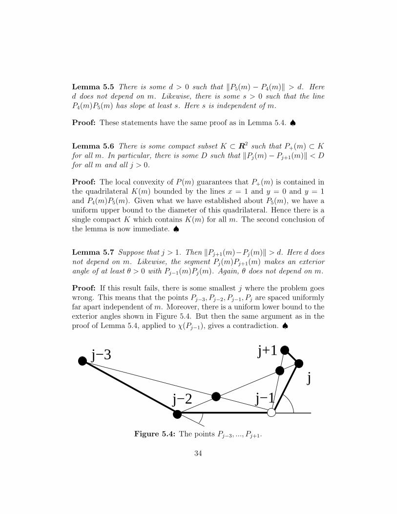
Lemma 5.7 Suppose that j > 1. Then ‖Pj+1(m)−Pj(m)‖ > d. Here d does

not depend on m. Likewise, the segment Pj(m)Pj+1(m) makes an exterior

angle of at least θ > 0 with Pj−1(m)Pj(m). Again, θ does not depend on m.

Proof: If this result fails, there is some smallest j where the problem goeswrong. This means that the points Pj−3, Pj−2, Pj−1, Pj are spaced uniformlyfar apart independent of m. Moreover, there is a uniform lower bound to theexterior angles shown in Figure 5.4. But then the same argument as in theproof of Lemma 5.4, applied to χ(Pj−1), gives a contradiction. ♠

j−3

j

j+1

j−1j−2

Figure 5.4: The points Pj−3, ..., Pj+1.

34

Lemma 5.8 Suppose that j > 1. The segment Pj(m)Pj+1(m) makes an

interior angle of at least θ > 0 with Pj−1(m)Pj(m). Here, θ does not depend

on m.

Proof: This is forced by the fact that every 5 consecutive points lie on aconvex pentagon, together with the uniform lower bound on the side lengths.♠

Corollary 5.9 The sequence {P+(m)} converges, at least on a subsequence,

to a strictly convex infinite polygonal path P+(∞). Every 5 consecutive points

of P+(∞) are the vertices of a strictly convex pentagon.

Proof: This follows immediately from the uniform bounds we have on allthe lengths and angles, together with compactness. ♠

5.4 Compactness Proof

Now we put everything together and prove Theorem 1.2. As we mentionedabove, it suffices to prove that the invariant Z = Z(n, k) has compact levelsets. Let {P (m)} be as in the previous section. These pentagram spirals allhave the same Z-invariant. Let X+(m) denote the portion of the triangula-tion associated to P (m) which is contained in the seed

S ′(m) = T 4k+4

n,k (S(m)). (22)

We use the seed S ′(m) rather than S(m) because our construction producesa union of triangles whose outermost portion is somewhat ragged.

We will show below that the sequence {X+(m)} converges to a triangula-tion which we will call X+(∞). There are two kinds of edges in X+(m). Theedges of the first kind are contained in P (m) and its images under powersof the pentagram map. The union of these edges will converge to strictlylocally convex paths in X+(∞). The second kind of edge in X+(m) is ashortest diagonal of P (m) or one of its images under powers of the penta-gram map. These edges of the second kind will converge to the correspondingshortest diagonals of the strictly convex paths in X+(∞) which we have justmentioned.

35

The convergence of triangulations implies that the sequence of seeds{S ′(m)} converges to a nontrivial seed S ′(∞). Indeed, the convex poly-gon A′ supporting S ′(∞) is just the outer boundary of the tiling X+(∞).Some of the edges of this outer boundary are edges of the first kind, andthese determine the B′ points marking k of the edges of A′. The convergenceof seeds implies the compactness result.

For ease of exposition we suppose k > 1. The case k = 1 is similar and infact easier. Each pentagram spiral P (m) is part of a system of k pentagramspirals P (m, j) for j = 1, ..., k, which are permuted by the pentagram map.

Figure 5.5: The image of P+(∞) under the pentagram map.

Let P+(∞, 1) be the limit guaranteed by Corollary 5.9. The pentagrammap is well defined on P+(∞, 1), starting from the first point onwards, as indi-cated by Figure 5.5. Let P+(∞, 2) be the image of P+(∞, 1) under the penta-gram map. Evidently, P+(∞, 2) is the limit of {P+(m, 2)}, where P+(m, 2) issome forward-infinite portion of P (m, 2). From our construction, we see thatP+(∞, 2) is a locally strictly convex infinite path. Moreover, every 5 consec-utive points of P+(∞, 2) are the vertices of a strictly convex pentagon. Butnow the pentagram map is defined on P+(∞, 2), and we arrive at P+(∞, 3),which is evidently the limit of a suitably defined sequence {P+(m, 3)}.

We continue this way until we reach P+(∞, k + 1). This is a proper sub-path of P+(∞, 1), where roughly n− k/2 vertices have been chopped off thefront. Let X ′

+(∞) denote the union of the paths P+(∞, j), for j = 1, ..., k,together with all their shortest diagonals. The corresponding union X ′

+(m)contains the tiling X+(m).

By construction, X ′

+(m) converges to X ′

+(∞). But then there is a subsetX+(∞) which is the limit of the slightly smaller X+(m). The outer boundaryof X+(∞) is the limit of the sequence {S ′(m)} of seeds. This convergence iswhat we had wanted to establish. The proof of Theorem 1.2 is done.

36

6 Geometry of the Tiling

6.1 Hilbert Diameter

Our goal in this chapter is to prove Theorems 1.3 and 1.4.Let K ⊂ RP

2 be a compact convex domain. Given 2 points b, c ∈ K, wehave the Hilbert distance

dK(b, c) = − log[a, b, c, d] (23)

where a and d are the two points where the line bc intersects ∂K, orderedas in Figure 6.1. This is a projectively natural metric on K. When K is acircle, dK is the hyperbolic metric in the Klein model.

dc

ba

Figure 6.1: The Hilbert distance

Suppose that L is a compact set contained in the interior of K. We definethe Hilbert diameter of L to be the diameter of L as measured in the Hilbertmetric.

Lemma 6.1 Suppose that {Ln} is a sequence of compact convex subsets con-

tained in the interior of K. Suppose that the Euclidean diameter of Ln con-

verges to the Euclidean diameter of K. Then the Hilbert diameter of Ln

converges to ∞.

Proof: Take a segment σm which connects two points on Lm which are max-imally spaced apart. Call these points bm and cm. Let am and dm be thepoints used in the definition of dK(am, bm). By construction ‖am − bm‖ and‖cm−dm‖ converge to 0 whereas ‖bm− cm‖ is uniformly bounded away from0. In this situation dK(bm, cm) → ∞. ♠

37

6.2 Support of the Tiling

Now we turn to the proof of Theorem 1.3. We begin with a corollary ofLemma 6.1.

Corollary 6.2 Suppose that {Km} is a nested family of compact convex sub-

sets, with Km+1 contained in the interior of Km for all m ∈ Z. Suppose that

there is some uniform constant C such that the Hilbert diameter of Km+1

with respect to Km is less than C for all m. Then⋂Km is a single point.

Proof: We just use the upper bound on diameter. Lemma 6.1 implies thatthe Euclidean diameter of Km+1 is at most λ times the Euclidean diameterof Km, for some uniform λ < 1. ♠

Now we turn to the triangulation X associated to a pentagram spiral P .We think of X as a union of solid triangles.

Let (A0, B0) be the seed generating P . Define

(Am, Bm) = Tmn(A0, B0). (24)

Let Km be the convex region bounded by the polygon Am. By construction,Km+1 is contained in the interior of Km.

By Theorem 1.2 and compactness, there is an upper bound C such thatthe Hilbert diameter of Km+1 with respect to Km is less than C, independentof m. Here we are using the projective naturality of the Hilbert metric. Thepoint is that we are just sampling a pre-compact subset of seeds in C(n, k).Corollary 6.2 now says that ⋂

Km (25)

is a single point. But X contains Km−Km+1. Hence X contains all points ofK0 except for this one interesection point. This is what we wanted to prove.

Next we claim that X is a triangulation of RP2 −L, where L is a single

line. This is equivalent to the statement that the ω limit set of P− is a singleline L. Here P− is the outward portion of P .

As is well known, projective dualities conjugate the (suitably interpreted)pentagram map to its inverse. Thus, the ω-limit set of P− is dual to the ω-limit set of P ∗

+, the inward part of the dual pentagram spiral. We havealready proved that the latter is a single point. Hence, the former is a singleline.

This completes the proof of Theorem 1.3.

38

6.3 Winding of Pentagram Spirals

Let P be a pentagram spiral, with distinguished vertex P1. We translate thepicture so that P ⊂ R

2 and so that the origin is the limit point and P1 is onthe positive x-axis, as shown in Figure 6.2.

1

P2

P3

Q2Q3

P1

Q

Figure 6.2: The spine

The vertex Q1 = P1 is the apex of a (shaded) cone C which contains theinward spiraling direction of P starting at P3. Hence C contains the limitpoint of P , namely the origin. The top edge of C leads to a point Q2 lying inthe upper half plane. The important point here is that arg(Q2) > arg(Q1).We can repeat the same construction at Q2. There is a cone which containsthe origin, and one of the edges of this cone leads to a point Q3 such thatarg(Q3) > arg(Q2).

39

Let P+ be the inward spiraling direction of P . Let Q+ be the polygonalpath connecting the points Q1, Q2, Q3, ... as shown in Figure 6.2. Both thesepaths converge to the origin in the forward direction. Since Q+ containsinfinitely many points and each such point lies on one of the finitely manyspirals in the tiling, we see that some spiral contains infinitely many point ofQ+. But, in fact, by inspecting the picture we see that whenever some pointof Q+ intersects a spiral, the next point of Q+ intersects the next spiral.Thus P+ and Q+ intersect infintely often.

Since the argument increases along both P+ and along Q+, we see thatthe argument increases by more than 2π along P+ between every two inter-sections with Q+. Hence, the argument along P+ increases without bound.This proves Theorem 1.4.

Remark: The proof of Theorem 1.4 is really quite simple. The only way itrelies on the previous material is that we would like to say that the pentagramspiral P really does have a single limit point.

40

7 Experiments and Discussion

7.1 Periodicity

With respect to specially chosen labeling schemes, the pentagram map is theidentity on C(5) and has period 2 on C(6). See [Sch1]. Referring to thepentagram spirals, I discovered the following result computationally.

Theorem 7.1 The following is true.

• T 24,1 is the identity on C(4, 1).

• T 24,2 is the identity on C(4, 2).

• T 85,1 is the identity on C(5, 1).

Theorem 7.1 says that all the pentagram spirals of this kind are self-projective. Theorem 7.1 can be expressed in terms of seeds and the seedmap, and so it only involves a finite number of points and lines. Thus,Theorem 7.1 can be established by a finite calculation, similar in spirit towhat is done in [ST]. I have not yet made the rigorous calculations. Some ofthe results in [ST] have conceptual proofs, and I wonder if there are likewiseconceptual proofs for the statements in Theorem 7.1

It seems discussing how I discovered this. My computer program allowsthe user to normalize the spirals so that the first 4 points are the vertices ofthe unit square. One can then watch an animation which shows the iterationof Tn,k. I put in an option which allows the user to choose a smallish integerq and watch the movie showing T q

n,k.For instance, for the parameter (n, k) = (4, 3) the choice q = 18 makes

for a nice movie. The point is that, for a random choice of pentagram spiralof type (4, 3), the 18th power of the shift map is fairly close to the identity,so an animation of the map looks somewhat like a flow to the naked eye. Asanother example, for (n, k) = (6, 2) the choice q = 54 often produces a nicemovie. I have found a few of these values experimentally, but not many. Thereader can see all of this in action on my program.

For the combinatorial type (4, 1), I noticed that the image on the com-puter screen, for q = 1 just flickered back and forth. When I put in q = 2the image was just stationary. Likewise, for the combinatorial type (4, 2),the choice q = 2 “froze the movie” and for the combinatorial type (5, 1)the choice q = 8 “froze the movie”. I would say that this is overwhelmingexperimental support for Theorem 7.1.

41

7.2 Asymptotic Shape

We can combine Theorem 7.1 with some of our other results to get moreinformation about the special cases (4, 1), (4, 2).

Theorem 7.2 Any PLC pentagram spiral of type (4, 1) of (4, 2) is projec-

tively equivalent to a self-similar polygonal path.

Proof: We can normalize by a projective transformation so that our penta-gram spirals lie in the plane and have the origin as their limit point. If P is apentagram spiral as in Theorem 7.1, then there is a projective transformationS so that S(P ) = P . Necessarily S preserves the ω-limit set of P . HenceS preserves the line at infinity and fixes the origin. That is, S is a lineartransformation.

Now, the action of S shifts the indices of P by 2, or 8 depending on thecase. In the cases (4, 1) and (4, 2) one can argue that the path made fromthe short diagonals of P again winds infinitely often around the origin. Butthis means that the orbits of S wind infinitely often around the origin. Butthen S is conjugate to a similarity. So, in the cases (4, 1) and (4, 2), thereis a canonical normalization of the pentagram spirals so that they are self-similar. ♠

The case (4, 1) yields a 1-parameter family of distinct shapes and the case(4, 2) yields a 2 parameter family of shapes. The argument above breaks downin the case (5, 1), but experimentally the result seems to be true.

To describe some experimental results along these lines, we need to in-troduce some terminology. Let Γ be an infinite polygonal path which limitson the origin in one direction and exits every compact set of the plane inthe other direction. We call Γ quasi-logarithmic (or QL for short) if thereis some nontrivial homothety D such that the family of curves {Dn(Γ)} isprecompact in the Hausdorff topology on shapes. To say that Γ is QL is tosay that Γ is only boundedly far from being invariant under a homothety.For instance, a logarithmic spiral is quasi-logarithmic.

I mentioned above that my computer program normalizes pentagram spi-rals so that 4 distinguished vertices are the vertices of a unit square. I alsoprogrammed things so that different normalizations are possible. For in-stance, one can normalize by a homothety so that the distinguished vertexis a point of the unit circle. If a particular pentagram spiral is QL, then the

42

movie shown with this alternate normalization would “go on forever” keepingmore or less the same shape.

It seems that for most choices of n and k, the pentagram spirals of type(n, k) are QL. For instance, when n ≤ 6, only the case (6, 1) seems to producepentagram spirals which are not QL. In general, it seems that the larger val-ues of k produces pentagram spirals which are more likely to be QL. I wouldneed to do more experiments before making a definitive conjecture on this,so let me just pose this as a question:

Question: Are there values (n, k) such that every PLC pentagram spiralis QL? If so, which values?

7.3 Logarithmic Pentagram Spirals

For each choice of (n, k) there is a self-similar pentagram spiral P which Icall the logarithmic pentagram spiral (or LPS for short.) The vertices of Plie in a logarithmic spiral and the edges of P are inscribed in a rotated copyof the logarithmic spiral. The pentagram map carres P to a rotated copy ofP .

The LPS can be normalized so that it has vertices {zn| n ∈ Z}, where

|z| < 1,2π

n+ k< arg(z) <

2π

n, (z + z)k = zn+k(1 + z)k. (26)

These equations come from the observation that the intersection of the linethrough 1 and z2 with the line through z and z3 is

w =z(z + z)

1 + z,

and that the combinatorics of the spiral dictate that wk = zn+2k. I had a lotof trouble solving Equation 26 on Mathematica, but I will describe a differentway to draw very close approximations to the LPS.

Say that the seed P = (A,B) is normalized if

A1 = (0, 0), A2 = (1, 0), A3 = (1, 1), A4 = (0, 1). (27)

That is, the first 4 vertices of P are the vertices of the unit square. Eachpoint of C(n, k) has a unique normalized representative. A normalized repre-sentative consists of a convex n-gon and k additional points. The locations

43

of these points can be described by the quantities

di =‖Ai −Bi‖

‖Ai − Ai+1‖∈ (0, 1), i = (n− k + 1), ..., n. (28)

The point An+1 is interpreted as A1.Given some point P = (A,B) ∈ C(n, k) and some integer j, we define

P j = (Aj, Bj) as the normalized version of T jn,k(P ). Given some integer m,

define Θm(P ) = (A′, B′), where A′ is the pointwise average of the polygonsA0, ...., Am−1 and the number d′j is the average of the corresponding num-bers for P 0, ..., Pm−1. In practice, Θm seems to act as a kind of contractionmapping on C(n, k), and the fixed point is the logarithmic pentagram spiral.

So, one can choose some smallish m and iterate Θm several times. Thisproduces a point in C(n, k) very close to the point representing the logarith-mic pentagram spiral. Given a point in C(n, k) representing the logarithmicpentagram spiral, one can then apply projective transformations to find bet-ter normalizations. The cheapest way to do this is just to apply Tn,k manytimes and then dilate the picture. This method produced the picture shownin Figure 7.1.

Figure 7.1: Approximation to the LPS of type (5, 3).

44

The logarithmic pentagram spiral is a natural origin for the space C(n, k)just as the projective class of the regular n-gon is a natural origin for thespace C(n). Computer experiments suggest the following conjecture

Conjecture 7.3 For any (n, k), the invariant Z is uniquely maximized, and

has a unique critical point, at the point representating the logarithmic penta-

gram spiral.

There is an analogous conjecture for the space C(n). Corollary 1.2 in mypaper [Sch4] proves that (the analogue of) Z is maximized at the regularpolygons when restricted to the subspace of polygons which are inscribed incircles.

7.4 Twisted Pentagram Spirals

The notion of a twisted polygon has been very useful in the study of theordinary pentagram map. See [Sch3], [OST1], and [OST2]. A twisted

n-gon is a map φ : Z → RP2 which intertwines translation by n with a

projective transformation M . That is,

φ ◦ µ = M ◦ φ(k), (29)

Here µ is translation by n. That is, µ(k) = k + n. The transformation M isthe monodromy of the twisted polygon.

The pentagram map acts on twisted n-gons and again commutes withprojective transformations. One can define 2n flag invariants of a twistedn-gon just as for an ordinary ones. The flag invariants of twisted n-gon andits iterates under the pentagram map naturally give rise to a labeling of T ,as in §4.2. This labeling is an element of T (n, 0).

Now we want to do the same kind of thing for pentagram spirals. Firstof all, we fix a model tiling generated by a particular element of C(n, k), saythe logarithmic pentagram spiral. (The model is just used for combinatorialpurposes.) Next, we create a locally identical tiling of the universal cover X̃of R2 − (0, 0). That is, we simply pull back the tiling to X̃. Let T̃ denotethe tiling of the universal cover.

The space X̃ is homeomorphic to the plane, but it has an exotic projectivestructure on it. A straight line in this universal cover is something whichprojects to a straight line. There is a Z-action on X̃, namely the deck

45

group. The deck group acts so as to carry lines to lines. Let µ be a generatorof the deck group. We have µ(T̃ ) = T̃ .

A twisted pentagram spiral is an adapted map φ satisfying Equation 29with respect to the deck group generator µ. By adapted map I mean that φis a homeomorphism when restricted to each (solid) triangle of T̃ and that φcarries each line segment in the 1-skeleton of T̃ to a straight line segment inRP

2. Note that some of these line segments consist of 3 consecutive edgesof triangles.

An ordinary pentagram spiral is simply a twisted pentagram spiral havingmonodromy the identity. Moreover, the above definition reduces to the usualdefinition in the case of closed polygons. It is merely the original definitionrephrased in terms of the triangulation produced by the pentagram map.

Some readers might not like the above geometric definition of a twistedpentagram spiral, so let me describe things algebraically. A projective equiv-alence class of A twisted pentagram spiral is nothing more than an elementof T (n, k). Starting with an element of T (n, k), one can start building anetwork of line segments in the projective plane, such that the correspond-ing flag invariants give the labels of T (n, k). As one develops the picturegoing “all the way around” the cylinder R2/Vn,k, one might observe that theconfiguration in the projective plane does not close up. The failure of thepicture to close up is encoded in the monodromy.

7.5 Integrability

Computer experiments suggest the following conjecture.

Conjecture 7.4 The map Tn,k acting on C(n, k) is a discrete totally inte-

grable system.

What I mean is that C(n, k) should have a singular foliation by tori,each equipped with a flat structure, such that each orbit of Tn,k is containedin a finite union of tori. Moreover, the restriction of a suitable power ofTn,k to each torus is a translation relative to the canonical flat structure.Such a structure would arise if C(n, k) had an invariant Poisson structureand sufficiently many commuting invariant functions. This how the torusfoliation arises in [OST1] and [OST2] for the pentagram map.

I will describe, to some extent, the computer experiments which lead tothis conjecture. The interested reader can do the experiments themselvesusing my program.

46

Let T be a PLC pentagram spiral, and let c(T ) denote the limit pointof the inward spiraling direction of T . If we normalize T so that the first 4vertices are the vertices of the unit square Q, then the point c(T ) ∈ R

2 is acanonical point associated to T . Assuming that T is a pentagram spiral oftype (n, k), we define

cm = c(Tmn,k(T )). (30)

That is, cm is the limit point of the mth iterate of T under the shift map.My computer program allows the reader to view the sequence {cm}.

For instance, the points {cm} seem to lie on a union of two (generically)smooth curve when (n, k) = (5, 2). When we consider the thinner sequence{c18n} in this case, we see points appearing in order on a smooth curve. Inother words, the movie we produce for the choices (n, k) = (5, 2) and q = 18shows the limit point gently rotating around a smooth curve. Again, weencourage the reader to download the program, so that he or she can see thisin action.

The space C(5, 2) is 4-dimensional. The experiments above suggest thatC(5, 2) is foliated by invariant loops and so that R2

5,2 preserves each loop inthe foliation and acts there as a (typically) irrational rotation. As is the casewith the pentagram map, one would describe this situation as “mildly hy-perintegrable”: The completely integrable situation would predict invariant2-tori.

As n and k increase, it is harder to see that the sequence {cm} is theprojection of a sequence of curves lying on a finite union of tori. However,for smallish values of m and k, one still gets a sense that this is the case.

7.6 Monodromy Invariants

The first step to proving the integrability conjecture is to find the integrals(i.e. invariants) of the map Tn,k. For the pentagram map, these invariants bynow have many constructions. I will describe the original way I thought ofthem. LetM be the monodromy of a twistedN -gon. If we replace the twistedN -gon by a projectively equivalent one, the monodromy M is replaced by aconjugate. However, the two quantities

Tr(M)

det1/3(M),

Tr(M∗)

det1/3(M∗). (31)

only depend on the projective equivalence class. In Equation 31 we thinkof M and M∗ as matrices representing the action of the monodromy on the

47

projective plane and on the dual projective plane respectively.The quantities in Equation 31 are rational functions of the flag invari-

ants. There is a certain natural weighting of the monomials in these rationalfunctions, and the homogeneous parts with respect to this weighting are themonodromy invariants. See [Sch3], [OST1] and [OST2] for details aboutthis.

The special weighting can be described as follows. If we take any elementof T (n, k) we can multiply all the forward slanting edges by s and all thebackward slanting edges by 1/s. This produces a new element of T (n, k). Allthe compatibility equations hold for the new equations. Every paper whichhas discussed the integrability of the pentagram map (and its generalizations)uses this scaling in a crucial way.

Now, the monodromy of a pentagram spiral can be computed using a pathwhich only encounters finitely many edges of the tiling T̃ . This, it would seemthat the quantities in Equation 31 would also be rational functions in finitelymany of the flag invariants. The scaling mentioned above works just finehere. So, the weighted homogeneous parts ought to be invariants of the mapTn,k on the larger space T (n, k), which we might as well interpret as the spaceof twisted pentagram spirals of type (n, k). Restricting these invariants tothe subset C(n, k) we would get invariants for the shift map Tn,k.

I tried to compute the monodromy invariants for the very modest case(n, k) = (4, 1) and I arrived at depressingly complicated expressions. Thismakes me somewhat pessimistic that one could arrive at crisp formulas likeEquation 31 in the general case. It seems to me that the calculation will haveto wait either for a more determined experimenter or for a better coordinatesystem.

My guess is that the Poisson bracket of [OST1] and [OST2] will gener-alize to the case of pentagram spirals as well. But I will leave this discussionfor a later paper.

48

8 References

[FM] V. Fock, A. Marshakov, Integrable systems, clusters, dimers and loop

groups, preprint, 2013

[GK] A. B. Goncharov and R. Kenyon, Dimers and Cluster Integrable Sys-

tems , preprint, arXiv 1107.5588, 2011.

[GSTV] M. Gekhtman, M. Shapiro, S.Tabachnikov, A. Vainshtein, Higherpentagram maps, weighted directed networks, and cluster dynamics, Electron.Res. Announc. Math. Sci. 19 21012, 1–17

[Gli] M. Glick, The pentagram map and Y -patterns, Adv. Math. 227, 2012,1019–1045.

[Gli1] M. Glick, The pentagram map and Y -patterns, 23rd Int. Conf. onFormal Power Series and Alg. Combinatorics (FPSAC 2011), 399–410.

[KDif ], R. Kedem and P. DiFrancesco, T -Systems with boundaries from net-

work solutions , preprint, arXiv 1208.4333, 2012

[KS] B. Khesin, F. Soloviev Integrability of higher pentagram maps, Mathem.Annalen. (to appear) 2013

[MB1] G. Mari Beffa, On Generalizations of the Pentagram Map: Discretiza-

tions of AGD Flows , arXiv:1303.5047, 2013

[MB2] G. Mari Beffa, On integrable generalizations of the pentagram map

arXiv:1303.4295, 2013

[Mot] Th. Motzkin, The pentagon in the projective plane, with a comment

on Napiers rule, Bull. Amer. Math. Soc. 52, 1945, 985–989.

[OST] V. Ovsienko, R. Schwartz, S. Tabachnikov, Quasiperiodic motion for

the pentagram map, Electron. Res. Announc. Math. Sci. 16 ,2009, 1–8.

[OST1] V. Ovsienko, R. Schwartz, S. Tabachnikov, The pentagram map:

A discrete integrable system, Comm. Math. Phys. 299, 2010, 409–446.

49

[OST2] V. Ovsienko, R. Schwartz, S. Tabachnikov, Liouville-Arnold inte-

grability of the pentagram map on closed polygons, to appear in Duke Math.J.

[Sch1] R. Schwartz, The pentagram map, Experiment. Math. 1, 1992, 71–81.

[Sch2] R. Schwartz, The pentagram map is recurrent, Experiment. Math.10, 2001, 519–528.

[Sch3] R. Schwartz, Discrete monodromy, pentagrams, and the method of

condensation, J. of Fixed Point Theory and Appl. 3, 2008, 379–409.

[Sch4] R. Schwartz, A Conformal Averaging Process on the Circle Geom.Dedicata., 117.1, 2006.

[Sol] F. Soloviev Integrability of the Pentagram Map, to appear in DukeMath J.

[ST] R. Schwartz, S. Tabachnikov, Elementary surprises in projective ge-

ometry, Math. Intelligencer 32, 2010, 31–34.

50