Penetration of solar radiation in the upper ocean: A

Penetration of solar radiation in the upper ocean:

A numerical model for oceanic and coastal waters

ZhongPing Lee,1,2 KePing Du,3 Robert Arnone,1 SooChin Liew,4 and Bradley Penta1

Received 20 October 2004; revised 11 March 2005; accepted 4 May 2005; published 27 September 2005.

[1] For studies of heat transfer in the upper ocean, the vertical distribution of solarradiation (ESR) in the shortwave domain plays an important role. In earlier studies, a sumof multiple exponentials was used to describe the vertical transmittance of ESR. For thoseexponential terms, an attenuation coefficient for each term is assigned, and thoseattenuation coefficients are assumed to be vertically constant. Furthermore, thoseattenuation coefficients are empirically modeled as functions of chlorophyll concentration(Chl) to cope with varying water properties of the oceans. Since attenuation coefficients ofocean waters are generally determined by components more than Chl alone, we developeda generalized model bypassing the use of Chl on the basis of extensive numericalsimulations. In this new model, vertical transmittance of ESR is separated into twoexponential terms, with one for the contributions of wavelengths below 700 nm (thevisible domain, EVIS) and one for wavelengths above 700 nm (the infrared domain, EIR).An attenuation coefficient is assigned for each of the two exponential terms. Unlike earliermodels, these attenuation coefficients vary with depth as expected. Furthermore, theattenuation coefficient for the visible domain is modeled as a function of water’sabsorption and backscattering coefficients. Since absorption and backscatteringcoefficients of the world oceans can be adequately derived from observations of oceancolor, the model we developed provides an effective and adequate means to describe thethree-dimensional variation of both EVIS and ESR in the upper layer of the world oceans.

Citation: Lee, Z., K. Du, R. Arnone, S. Liew, and B. Penta (2005), Penetration of solar radiation in the upper ocean: A numerical

model for oceanic and coastal waters, J. Geophys. Res., 110, C09019, doi:10.1029/2004JC002780.

1. Introduction

[2] For studies of heat transfer in the upper ocean, it isimportant to reliably provide shortwave solar radiation (ESR,see Table 1 for terms used in this text) in the upper watercolumn [Zaneveld et al., 1981; Lewis et al., 1990]. Knowl-edge of this vertical distribution of ESR requires informationof ESR at the surface and how ESR attenuates with depth (z).The total ESR incident on the water surface can now beestimated with models or measurements made from space[Gregg and Carder, 1990;Mueller et al., 2004]. This energycan be considered as two separate portions: energy withwavelengths less than 700 nm (visible domain, EVIS), andenergy with wavelengths greater than 700 nm (infrareddomain, EIR). The attenuation coefficient for EIR is almostcompletely dominated by water absorption; thus this atten-

uation can be viewed as invariable to changes of waterconstituents [Morel and Antoine, 1994]. Also, because ofthe enormously large absorption coefficients of water mol-ecules, this portion of solar radiation is quickly lost in theupper 3 m [Morel and Antoine, 1994].[3] EVIS encompasses the wavelengths shorter than

700 nm. The pioneer study of Zaneveld et al. [1981] andsubsequent studies [Chang and Dickey, 2004; Kara et al.,2005; Kirk, 1988; Lewis et al., 1990; McClain et al., 1996;Morel and Antoine, 1994; Ohlmann et al., 2000; Schneiderand Zhu, 1998; Siegel et al., 1995] have demonstrated thatthe penetration of EVIS in the upper layer of the ocean playsan important role in heat transfer and sea surface tempera-ture. Unlike the attenuation coefficient for EIR, however, theattenuation coefficient for EVIS changes horizontally withconstituents in the water [Jerlov, 1976; Morel and Antoine,1994; Zaneveld et al., 1981]. Detailed horizontal informa-tion regarding the attenuation coefficient of EVIS is requiredto determine the global distribution of EVIS(z).[4] In the past two decades, multiple exponential terms

[Paulson and Simpson, 1977; Simpson and Dickey, 1981;Zaneveld and Spinrad, 1980] were generally used todescribe the vertical distribution of EVIS or ESR (morereviews can be found in work by Morel and Antoine[1994] and Ohlmann and Siegel [2000]). For these expo-nential terms, an attenuation coefficient (or attenuationdepth) is assigned for each term. These attenuation coef-

JOURNAL OF GEOPHYSICAL RESEARCH, VOL. 110, C09019, doi:10.1029/2004JC002780, 2005

1Naval Research Laboratory, Stennis Space Center, Mississippi, USA.2Also visiting professor at Ocean Remote Sensing Institute, Ocean

University of China, Qingdao, China.3State Key Laboratory of Remote Sensing Science, Research Center for

Remote Sensing and Geographic Information Science, School ofGeography, Beijing Normal University, Beijing, China.

4Center for Remote Imaging, Sensing and Processing, NationalUniversity of Singapore, Singapore.

This paper is not subject to U.S. copyright.Published in 2005 by the American Geophysical Union.

C09019 1 of 12

ficients are kept vertically constant, but horizontally varywith Jerlov [1976] water types. Dividing waters into differ-ent types is coarse and qualitative, where the attenuationcoefficient associated with a water type is a rough estima-tion. Furthermore, variations of attenuation coefficientswithin a water type are ignored, and sharp steps betweenadjacent water types result. In the last decade, advancementin remote sensing of ocean color by satellite has providedfine-scale measurements of optical and biological propertiesfor the world oceans. Therefore models that incorporatethese valuable observations better fit the studies of solarheating on global scales.[5] At present, advanced numerical models [Gordon et

al., 1975; Liu et al., 2002; Mobley, 1995; Morel and Gentili,1991] have been developed to accurately simulate thesubsurface light field with known water properties andboundary conditions. These models, which are excellentfor studying the general trend, are impractical for three-dimensional global models because of their computationalinefficiency. Simple and efficient models, but withoutsignificant loss of accuracy, are required.[6] On the basis of the strategy of case 1 and case 2 water

separation [Morel and Prieur, 1977], simple and explicitmodels have been developed to incorporate satellite-derivedchlorophyll concentrations (Chl) into the description of thehorizontal and vertical distributions of solar radiation. Amodel for the spectral diffuse attenuation coefficients(Kd(l)) has been specifically developed for the spectrallyresolved EVIS, or so-called downwelling spectral irradiance(Ed(l)), with values of Kd(l) described as empirical func-tions of Chl [Morel, 1988; Morel and Maritorena, 2001].When Chl values are provided via satellite observationsof ocean color [Carder et al., 1999; Gordon and Morel,1983] (see also Ocean color algorithm evaluation, availableat http://oceancolor.gsfc.nasa.gov/REPROCESSING/SeaWiFS/R3/), Kd(l) of ocean waters can be evaluated fordesired wavelengths. When this information and surfaceEd(l) are provided, Ed(l, z) at desired depths can be easilycalculated [Gordon et al., 1980], as can EVIS(z), the spectral

integration of Ed(l, z) (see Table 1). Note that for theultraviolet to visible domain, the number of wavelengthscan be more than 100 for fine spectral resolution.[7] Although this wavelength-resolved approach might

be required for studies of phytoplankton photosynthesis[Sathyendranath et al., 1989a], it is found ‘‘superfluouswhen dealing with the heating rate’’ [Morel and Antoine,1994], and computationally expensive for fine-scale three-dimensional modeling of the global oceans. To increase thecomputation efficiency, without significant loss of accuracy,efforts have been made to simplify the process of modelingthe vertical transmittance of EVIS. For this purpose, trans-mittance of EVIS is usually simplified to a few exponentialfunctions, with a partition factor and an ‘‘effective attenu-ation’’ coefficient assigned for each term [Morel andAntoine, 1994; Ohlmann and Siegel, 2000]. Furthermore,these partition factors and attenuation coefficients areexpressed as functions of Chl, and/or cloudiness ratios[Morel and Antoine, 1994; Ohlmann and Siegel, 2000].Therefore when Chl values and other auxiliary information(such as Sun angle) are available, vertical distribution ofEVIS can be quickly provided and efficiently incorporatedinto physical models.[8] However, these models or strategies work only for

case 1 waters, where all optical properties are determined byChl alone (with solar zenith angle explicitly or implicitlyincluded) [International Ocean-Colour CoordinatingGroup, 2000; Morel, 1988]. Since ocean waters havevarious combinations of biological and chemical constitu-ents [Bricaud et al., 1981; Stramski et al., 2001], theglobally averaged bio-optical relationship could result inbig uncertainties for a specific region or a specific time.Fundamentally this is due, first, the optical properties ofocean waters being generally determined by at least threeindependent variables [Sathyendranath et al., 1989b]: phy-toplankton, colored dissolved organic matter (CDOM), andsuspended sediments. In many cases knowledge of chloro-phyll concentration alone is inadequate to accurately quan-tify the attenuation coefficients, an optical property. Second,

Table 1. Terms and Definitions

Definition Units

a(l) absorption coefficient at wavelength l m�1

bb(l) backscattering coefficient at wavelength l m�1

Chl concentration of chlorophyll mg m�3

Ed(l, z) spectral downwelling irradiance at depth z W m�2 nm�1

EIR(z) downwelling solar radiation for wavelengths in the range of

700–2500 nm, =

Z 2500

700

Ed(l, z)dl

W m�2

EVIS(z) downwelling solar radiation for wavelengths in the range of

350–700 nm, =

Z 700

350

Ed(l, z)dl

W m�2

ESR(z) downwelling solar radiation at depth z, = EVIS(z) + EIR(z) W m�2

Kd(l) diffuse attenuation coefficient for Ed(l, z) at l m�1

K̂VIS(z) attenuation coefficient for EVIS(z) between 0 m and depth z m�1

K̂IR(z) attenuation coefficient for EIR(z) between 0 m and depth z m�1

TVIS(z) vertical transmittance of EVIS(z), = EVIS(z)/EVIS(0�) –

TIR(z) vertical transmittance of EIR(z), = EIR(z)/EIR(0�) –

T(z) vertical transmittance of ESR(z), = ESR(z)/ESR(0�) –

FVIS EVIS(0�)/ESR(0

�) –IOP inherent optical properties, mainly referring to the absorption

and backscattering coefficients in this paperm�1

rD subsurface irradiance reflectance –rF surface Fresnel reflectance –qa (qw) solar zenith angle above (below) the surface deg

C09019 LEE ET AL.: ATTENUATION OF SOLAR RADIATION

2 of 12

C09019

even for chlorophyll dominated waters, the attenuationcoefficient can differ significantly from one time to anotheror one place to another because of the ‘‘package effect’’[Bricaud and Morel, 1986; Kirk, 1994]. These naturalvariations put significant limitations on the attenuationcoefficients calculated on the basis of Chl, and then onthe resulting vertical distribution of EVIS.[9] To avoid such limitations associated with Chl-based

models, efforts have also been made to model the verticaltransmittance of EVIS as a function of water’s opticalproperties. In an earlier study based on field measurements,Zaneveld et al. [1993] modeled the attenuation coefficientof EVIS as a linear function of the diffuse attenuationcoefficient at 490 nm. Dividing EVIS of the upper watercolumn into three consecutive layers, separate empiricalcoefficients were developed for each layer [Zaneveld et al.,1993]. These coefficients, however, remain the same withineach layer, which thus cannot represent the steeper thanexponential reduction of EVIS in the subsurface layer[Zaneveld and Spinrad, 1980]. Later, Barnard et al.[1999], on the basis of 30 measurements made aroundCalifornia waters, modeled the attenuation coefficient ofEVIS as a polynomial function of depth and absorptioncoefficient at 490 nm. This empirical model, however, didnot consider the effects of scattering and was based on arelatively narrow range of water properties. Its applicabilityto broader range of waters, especially where scattering bysuspended sediments could be important in determining thelight field, is unclear [Barnard et al., 1999].[10] Realizing that water’s absorption (a) and backscat-

tering coefficients (bb) can be routinely measured in thefield and/or well retrieved from ocean color remote sensing[Hoge and Lyon, 1996; Lee et al., 2002; Loisel et al., 2001;Lyon et al., 2004], it would be very useful if a generalizedmodel for the attenuation of EVIS(z) can be developed thatuses values of a and bb as inputs. To reach this goal, wecarried out extensive numerical simulations by HydroLight[Mobley, 1995; Mobley et al., 2002], and developed asimple model for K̂VIS(z), the vertical attenuation coefficientof EVIS, with a, bb, and z as variables. Combined with themodel for EIR(z), a model with two exponentials is devel-oped for the vertical distribution of ESR(z). With this modeland images of a and bb provided by satellite remote sensing,three-dimensional ESR(z) in the upper ocean can then beefficiently calculated and implemented into models for heattransfer studies. Separately, EVIS(z) can be incorporated intophotosynthesis models [Behrenfeld and Falkowski, 1997] tostudy primary productivity in the oceans.

2. Vertical Transmittance of EIR

[11] As in the work by Morel and Antoine [1994], ESR(z)is partitioned into two portions: EVIS(z) (350–700 nm) andEIR(z) (700–2500 nm):

ESR zð Þ ¼ EVIS zð Þ þ EIR zð Þ: ð1Þ

The split is selected at 700 nm instead of 750 nm [Moreland Antoine, 1994] to accommodate outputs and modelscommonly used in physical and biological studies [Greggand Carder, 1990; Kirk, 1994; Morel, 1978; Zaneveld et al.,1993]. This difference is simply a practical choice, and is

not fundamentally different from that of Morel and Antoine[1994]. In addition, the split at 700 or 750 nm makes nodifference in simulating ESR(z), as long as it is by the sameapproach, though a slightly different set of model constantswould result.[12] The vertical distribution of the two components in

equation (1) are described by two separate exponentialfunctions,

EVIS zð Þ ¼ EVIS 0�ð Þe�K̂VIS zð Þz ð2aÞ

EIR zð Þ ¼ EIR 0�ð Þe�K̂IR zð Þz: ð2bÞ

Here K̂VIS(z) and K̂IR(z) in equation (2) are not the values atdepth z (so-called local value), but a spatial average between0 m and z. Also, K̂VIS(z) and K̂IR(z) are spectrally averageddiffuse attenuation coefficients that are weighted by thespectral irradiance in the visible and in the infrared,respectively. Both K̂VIS and K̂IR vary with depth and Sunangle.[13] Since water’s absorption coefficients are extremely

large in the infrared domain [Morel and Antoine, 1994], K̂IR

is considered independent of changes in water constituents.Also, as most of the solar radiation in this domain isabsorbed within the layer of top 3 m, Morel and Antoine[1994] treated K̂IR independent of z. Here we moved onestep further to resolve the vertical variation of K̂IR. For thisdevelopment, we first calculated K̂IR(z) as was done byMorel and Antoine [1994],

K̂IR zð Þ ¼ 1

zln

Z 2500

700

Ed l; 0�ð ÞdlZ 2500

700

Ed l; 0�ð Þe�aw lð Þz= cos qwð Þdl

0BBB@

1CCCA; ð3Þ

with qw the subsurface solar zenith angle. aw(l) is theabsorption coefficient of water in the range of 700–2500 nm, with values taken from Smith and Baker [1981]and Morel and Antoine [1994]. Ed(l, 0

�) is estimated fromMODTRAN 4 with standard marine aerosols (morecommon for the this study). The effect of aerosol type onthe calculated K̂IR is small (�10% for z = 0.5 m and �7%for z = 2.0 m) even when Ed(l, 0

�) estimated using strongcontinental aerosols.[14] From equation (3), values of K̂IR(z) in the layer of

0.01–3.0 m (for z deeper than 3 m, EIR is negligible)are calculated, with Sun angle (qa) varying from 0–60�(equivalent to qw from 0 to 40�) from zenith. From theseK̂IR(z), we found that K̂IR(z) can be described as

K̂IR z; qað Þ ¼ 0:560þ 2:304

0:001þ zð Þ0:65

" #1þ 0:002qað Þ: ð4Þ

Figure 1 presents examples of equation (4) modeled K̂IR(z)versus equation (3) calculated K̂IR(z), with an average errorof �3.0%. Clearly, for a change of 2 orders of magnitude ofK̂IR(z) in the surface layer, equation (4) represents thevertical variation of K̂IR(z) very well.[15] Studies [Pegau et al., 1997; Pegau and Zaneveld,

1993] have found that values of aw(l) in the infrared


3 of 12

C09019

domain vary with temperature and salinity, with thetemperature effect greater than the salinity effect. Thistemperature effect is found generally within �10% ofaw(l) for a temperature range of 0�C to 30�C, and thelarger effects only happened at a few wavelengths (such as750 nm) [see Pegau et al., 1997]. Since K̂IR(z) representsthe spectrally integrated attenuation in the wavelength rangeof 700–2500 nm, the temperature effect at a few wave-lengths is considered insignificant to K̂IR(z). Thereforevalues presented in equation (4) should be applicable towaters with temperature and salinity widely observed in theoceans.

3. Vertical Transmittance of EVIS

[16] For the visible domain, K̂VIS varies not only withdepth (the vertical direction), but also with water constitu-ents (the horizontal direction). In order to cope with thisthree-dimensional change of K̂VIS,Morel and Antoine [1994]expressed the vertical transmittance of EVIS (represented byTVIS) as

TVIS zð Þ ¼ EVIS zð ÞEVIS 0�ð Þ ¼

X2i¼1

vie�kiz: ð5Þ

Here vi and ki are parameters for TVIS and are constants fordifferent depths. For these multiexponential models, thevalues of vi and ki are further expressed as 5-orderpolynomial functions of log(Chl) [Morel and Antoine,1994]. Therefore given Chl and z, values of TVIS(z) can bequickly evaluated.[17] As stated earlier, water’s optical properties are gen-

erally determined by constituents not limited to Chl, butalso by CDOM and suspended sediments [Sathyendranathet al., 1989b]. Furthermore, Chl values derived from remotesensing of ocean color are not as reliable as those ofabsorption and backscattering coefficients [Lee et al.,2002; Lyon et al., 2004]. To get more accurate verticaldistribution of EVIS, an efficient and reliable approach is toestimate K̂VIS (an optical property) directly from water’s

inherent optical properties (IOP) [Preisendorfer, 1976]. Acomprehensive model is thus needed to describe the changeof K̂VIS for different optical properties and different depths.To develop such a model, concurrent data containing widerange of K̂VIS(z) and the corresponding optical properties arerequired. In an approach similar to Ohlmann and Siegel[2000], we used HydroLight to generate appropriate datasets. From the HydroLight data sets, we developed a modelto describe K̂VIS as a function of water’s inherent opticalproperties and depth. Such a model, combined with avail-able optical properties from satellite measurements, can beapplied for studies of heat transfer and photosynthesis inglobal oceans.

4. Numerical Simulations to Obtain K̂VIS(zzz)

[18] As in earlier studies [Morel and Antoine, 1994;

Ohlmann and Siegel, 2000], K̂VIS(z) is first derived fromnumerically simulated EVIS(z) that corresponds to a widerange of optical properties. As described by Ohlmann andSiegel [2000], simulation of Ed(z, l) is carried out byHydroLight. Unlike the simulations of Ohlmann and Siegel[2000] where water’s IOPs were determined by Chl only,IOPs in our simulations were simulated with varying Chland independently varying CDOM and suspended sedi-ments, as described by Lee et al. [2002] and InternationalOcean-Colour Coordinating Group/Ocean Colour AlgorithmGroup (Model, parameters, and approaches used to generatewide range of absorption and backscattering spectra, 2003,available at http://www.ioccg.org/groups/OCAG_data.html). Later, K̂VIS(z) is modeled as a function of totalabsorption and backscattering coefficients. This way, theconcentrations of Chl, CDOM, and sediment are no longerrequired, as long as accurate total absorption and backscat-tering coefficients are provided. In natural waters, for thesame optical properties, it is common to have differentconcentrations of Chl, CDOM, and sediments.[19] For numerical simulations by HydroLight, numerous

descriptions can be found in the literature [Berwald et al.,1995; Lee et al., 1998;Mobley et al., 1993, 2002;Morel andLoisel, 1998]. The following summarizes the input settingscarried out in this study.[20] 1. The downwelling irradiance at sea surface from

the Sun and sky is simulated by the spectral model of Greggand Carder [1990]. A wind speed of 5 m/s is assigned. Sunangles were at 10�, 30�, and 60� from zenith, respectively,with a clear sky.[21] 2. To determine the light field within the upper water

column, HydroLight requires information of water’s IOPs.For the attenuation coefficient of downwelling irradiance(the focus of this study), the important IOPs are the totalabsorption (a) and backscattering coefficients (bb), as thisattenuation is relatively insensitive to the scattering phasefunction of particles when values of a and bb are fixed [Leeet al., 2005a]. Chl values ranging from 0.03 to 30.0 mg/m3

(20 scales with a roughly 50% increasing rate) were used asone free parameter in order to provide a wide range ofoptical properties. Similar to earlier numerical studies[Gordon, 1989; Kirk, 1991; Morel and Loisel, 1998], allIOPs were kept vertically constant in this study.[22] 3. Total absorption coefficients were expressed as a

sum of the contributions of pure water, phytoplankton

Figure 1. Example of modeled K̂IR(z) (equation (4), opendiamonds) compared with calculated K̂IR(z) (equation (3),solid diamonds), with the Sun at 50� from zenith.


4 of 12

C09019

pigments, and CDOM (including detritus). Values of purewater absorption coefficient were taken from Pope and Fry[1997], with the pigment absorption coefficient determinedby Chl values [Bricaud et al., 1995]. Similar to Lee et al.[2002], five different CDOM absorption coefficients foreach Chl value were randomly assigned, with the ratio ofCDOM absorption to pigment absorption at 440 nm in arange of 0.5 to 5.0 (resulted in a range of 0.017–3.2 m�1 fora(440)).[23] 4. Scattering is separated into molecular and nonmo-

lecular (collectively called particle) components [Gordonand Morel, 1983; Morel and Gentili, 1993; Sathyendranathet al., 2001], with the molecular scattering coefficient takenfrom Morel [1974]. As described in Lee et al. [2002], theparticle scattering coefficient at 550 nm varied with Chl in arandom fashion. The phase function for particle scattering isthe average from Petzold’s measurements [Mobley et al.,2002]. With these different combinations of Sun angles andwater properties, a total of 300 (20 (Chl) � 5 (CDOM andparticle) � 3 (Sun angles)) HydroLight runs were carriedout.[24] 5. HydroLight simulations were performed for l in the

range of 350–700 nm with a 10-nm spectral resolution. Forthe same set of optical properties and boundary conditions,sensitivity tests with HydroLight run at a 5-nm resolutionshowed negligible (<1%) effects on TVIS(z) (not presented).[25] 6. Five geometric depths (excluding 0 m) were

selected for each HydroLight run, with depths spread withinand beyond the euphotic zone [Kirk, 1994]. Before initiat-ing HydroLight, a preliminary estimation was made todecide the deepest depth (zd) for each simulation. This zdis corresponding to �10�3 of Ed(l, 0�), with l thewavelength with lowest attenuation coefficient (the deepestpenetration wavelength) for that spectrum. This 0 to zdwater ‘‘slab’’ is then sliced into five consecutive layers. Forthe five layers with zi equal to the position of the bottom ofeach layer, EVIS(zi)/EVIS(0

�) span a range of � 0–80%. In

these HydroLight simulations, corresponding to the differ-ent optical properties, the first (z1) (and last, z5) depths ofthe layers ranged from 1.8 (147.4) m for the low absorptioncase to 0.2 (13.7) m for the high-absorption case.[26] 7. Bottom reflectance and inelastic scatterings (such

as Raman scattering) are excluded as they are beyond thescope of this study. Inelastic scattering makes negligiblecontributions to heat transfer and photosynthesis in thewater column [Morel and Gentili, 2004].[27] Note that the light field is actually determined by the

absorption and scattering properties [Mobley et al., 2002],the bio-optical models and the Chl values used in theHydroLight simulations merely provide a wide range ofinputs for the numerical simulations [Kirk, 1991].

5. Variation of K̂VIS and Its Modeling

[28] From HydroLight simulated EVIS(z), K̂VIS(z) is cal-culated through

K̂VIS zð Þ ¼ 1

zln

EVIS 0�ð ÞEVIS zð Þ

� �: ð6Þ

Figure 2 presents examples of K̂VIS(z) for a few cases. Notsurprisingly, for vertically homogeneous water, K̂VIS(z) stillchanges a lot (greater than a factor of two) in the subsurfacelayer. Also, K̂VIS(z) differs significantly for varying waterproperties. All these variations are the fundamental reasonsfor the multiple exponentials used to cope with the steepreduction of EVIS(z) below the surface. When a verticallyconstant value is used to replace K̂VIS(z), it will result inoverestimation of EVIS for the near-surface layer andunderestimation of EVIS for deeper depths. To accuratelydescribe the vertical distribution of EVIS that is needed forstudies of heat transfer and photosynthesis, it is important toknow and model the vertical variation of K̂VIS(z).[29] For each individual K̂VIS(z) profile, we found that it

could be well reproduced by a two-parameter model,

K̂VIS IOP; zð Þ ¼ K1 IOPð Þ þ K2 IOPð Þ1þ zð Þ0:5

: ð7Þ

Here K1 and K2 are model parameters with K1 for theasymptotic value at greater depths and K2 more important tothe subsurface K̂VIS value. IOP here represents combina-tions of different inherent optical properties. K1 and K2 inequation (7) do not vary with depth but vary with IOP. Thedotted lines in Figure 2 show equation (7) modeled K̂VIS(z)for those examples. Figure 3 presents the result ofHydroLight K̂VIS(z) versus equation (7)–modeled K̂VIS(z),for HydroLight simulations with the Sun at 30� from zenith.For the simulated data that K̂VIS(z) ranged from 0.04–1.6 m�1, the average error between HydroLight K̂VIS(z) andequation (7)–modeled K̂VIS(z) is 2.2% (maximum error is6.4%). Such results clearly demonstrate that equation (7) isadequate to describe the vertical change of K̂VIS(z). Thus thevertical profile of TVIS(z) can be modeled by a singleexponential function with two parameters (K1 and K2).[30] For this single exponential term, however, K̂VIS(z)

varies with both z and IOP. For global models to incorporatethe smooth distributions of water properties obtained fromsatellite observation of water color, it is necessary to spell

Figure 2. Examples of K̂VIS(z) for different water proper-ties. The numbers in the inset are values of a(490) andbb(490), respectively. Squares, diamonds, and circlesrepresent K̂VIS(z) from HydroLight simulations, whiledotted lines are models from equation (7) (see text fordetails).


5 of 12

C09019

out how K1,2 vary with water’s optical properties, as well aswith solar zenith angle. For K̂VIS(z) obtained from Hydro-Light simulations with the Sun at 30� from zenith, Figure 4shows the variations of K1,2 versus total absorption coef-ficients at 440 nm and 490 nm. These results show apositive correlation between K1,2 and a(440, 490), respec-tively. Since K1,2 also varies with backscattering coeffi-cients (not shown), values of K1,2 (and then K̂VIS(z)) cannotbe well predicted from a(440, 490) alone (see Figure 4).These features, however, suggest that K1,2 can be modeledas functions of both total absorption and backscatteringcoefficients.[31] Since K1,2 are cumulative effects of absorption and

scattering in the visible domain, there could be many waysto model K1,2 with different combinations of inputs. Asimple approach, as suggested by Zaneveld et al. [1993]and Barnard et al. [1999], is to use absorption and back-scattering coefficients at one spectral band, where data fromsatellite measurements are also available, to model K̂VIS(z).For this approach, we tried to model K1,2 using the values at

440 and 490 nm as inputs, respectively, and found usingvalues at 490 nm provided a slightly better result. Thereforeempirical models for K1,2 are obtained, with

K1 IOPð Þ ¼ c0 þ c1 a 490ð Þð Þ0:5þ c2bb 490ð Þ ð8aÞ

K2 IOPð Þ ¼ z0 þ z1a 490ð Þ þ z2bb 490ð Þ: ð8bÞ

Now, the values of c0,1,2 and V0,1,2 are independent of bothdepth and water properties, though they may still vary withsolar zenith angle.[32] To observe the variations of K1,2 for different solar

zenith angles, values of K1,2 from HydroLight simulationswith the Sun at 10� and 60� from zenith were analyzed.These results suggested that K1 only varies slightly fordifferent solar zenith angles, as expected from the asymp-totic theory [Zaneveld, 1989]. More variations with Sunangles were found for K2– the parameter important forsubsurface solar radiation. On the basis of these K1,2 valuesfrom HydroLight simulations, equation (8) is expanded toinclude Sun angle dependence,

K1 IOP; qað Þ ¼ c0 þ c1 a 490ð Þð Þ0:5þ c2bb 490ð Þh i

1þ a0 sin qað Þð Þ

ð9aÞ

K2 IOP; qað Þ ¼ z0 þ z1a 490ð Þ þ z2bb 490ð Þ½ a1 þ a2 cos qað Þð Þ:ð9bÞ

Note that qa is the solar zenith angle above the surface. Withthis model, the final mathematic function for TVIS(z) became

TVIS IOP; z; qað Þ ¼ e�K̂VIS IOP;z;qað Þz: ð10Þ

By fitting TVIS values from HydroLight simulations with thecombination of equations (7), (9), and (10), values ofparameters c0,1,2, V0,1,2, and a0,1,2 are derived (provided inTable 2) by least squares curve fitting, as done in earlierstudies to derive model parameters [Morel and Antoine,

Figure 3. K̂VIS(z) from model (equation (7)) comparedwith K̂VIS(z) from HydroLight (30� solar zenith angle),indicating that K̂VIS(z) can be well described by equation (7)with two parameters.

Figure 4. Values of (a) K1 and (b) K2, which are model parameters for K̂VIS(z), versus absorptioncoefficients at 440 nm and 490 nm.


6 of 12

C09019

1994; Ohlmann and Siegel, 2000]. Figure 5 presentsequation (10) modeled TVIS(IOP, z, qa) versus TVIS(IOP, z,qa) determined from HydroLight simulations. For those TVISvalues (limiting to the range of �0.001 to 0.8), bigger errorshappened at TVIS < 0.003, where the effects of EVIS on heattransfer and photosynthesis in the water column are small.For TVIS > 0.003, the average error is �9%. These resultsindicate that the simple, optical property-based, model(equation (10)) is adequate for describing the vertical profileof EVIS(z) for different waters.

6. Improvement Over Chl-Based Models

[33] On the basis of equations (1) and (2), the verticaltransmittance (= ESR(z)/ESR(0

�)) for shortwave solar radi-ation is

T IOP; z; qað Þ ¼ FVISe�K̂VIS IOP;z;qað Þz þ 1� FVISð Þe�K̂IR z;qað Þz; ð11Þ

with K̂VIS and K̂IR provided by equations (7) and (4),respectively. Here FVIS is the ratio of EVIS(0

�)/ESR(0�), and

its value is around 0.424 [Mobley, 1994] when the solarradiation is split at 700 nm. Equation (11) is similar to thewidely used model of Paulson and Simpson [1977, 1981].The attenuation coefficients in the two models, however, arefundamentally different. The attenuation coefficients inequation (11) vary with depth as suggested from radiativetransfer, while they are vertically constant in work byPaulson and Simpson [1977].

[34] In order to test the performance of this model andearlier models, a ‘‘standard’’ T(z) data set is generated,which is

T zð Þ ¼ FVISTVIS zð Þ þ 1� FVISð ÞTIR zð Þ; ð12Þ

with TVIS(z) created by HydroLight simulations and TIR(z)on the basis of equation (3). The HydroLight simulationswere run with Chl ranged from 0.03–30 mg/m3, but withcompletely different absorption and scattering coefficientsas compared to those described in section 4. The depths arefixed at 1, 2, 5, 10, 20, and 50 m, that is, within thecommonly observed surface mixed layer. Also, the Sunangle is set at 45� from zenith. Figure 6 shows the values ofChl and a(490) that are used as inputs to these HydroLightsimulations and to the T(z) models. The dotted line in Figure6 represents case 1 a(490) for those Chl values. Clearly, thedata set follows the pattern commonly observed in the field[Gordon and Morel, 1983; Morel, 1988].[35] There are two earlier models that can provide T(z) for

given Chl and z. One is that of Morel and Antoine [1994](MA94 hereafter), where T(z) is described as a sum of threeexponentials; another is that of Ohlmann and Siegel [2000](OS00 hereafter), where T(z) is evaluated from a sum offour exponentials. For this standard data set, since values ofChl (so do a(490) and bb(490)) are known, T(z) can bepredicted from these models. These T(z) can then becompared to each other, and to the standard data set.[36] The MA94 model has the same mathematical for-

mulation as equation (12), but the wavelength range is from300 to 2750 nm and the separation of visible and infrared isat 750 nm. Since solar irradiance at the sea surface in therange of 300–350 nm and 2500–2750 nm are only about1% of the total irradiance, we applied the model parametersofMorel and Antoine [1994] to the standard data set withoutany change. The split at 750 nm makes the FVIS valuedifferent from the FVIS value split at 700 nm, and a value of0.56 [Morel and Antoine, 1994] is used when applied to theMA94 model.

Figure 5. TVIS(z) from model (equation (10)) comparedwith TVIS(z) from HydroLight for three Sun angles.

Table 2. Values of the Model Parameters for K̂VIS(z)

Parameter Value

c0, m�1 –0.057

c1 0.482c2 4.221V0, m

�1 0.183V1 0.702V2 –2.567a0 0.090a1 1.465a2 �0.667

Figure 6. Values of a(490) and Chl used in section 6 formodel testing. The dotted line is case 1 a(490) for those Chlvalues, derived on the basis of the Kd(490) model of Morel[1988], and a(490) is approximated as 0.9 Kd(490).


7 of 12

C09019

[37] The OS00 model (equation (3) of Ohlmann andSiegel [2000]) is developed for the ratio of net irradianceflux, that is,

T 0 zð Þ ¼ ESR zð Þ � Eu zð ÞESR 0þð Þ ; ð13Þ

where Eu(z) is the upwelling irradiance at depth z, and T0(z)is modeled as a sum of four exponentials similar toequation (5). Compared to T(z) defined by Morel andAntoine [1994] and in this study, there is

T zð Þ ¼ T 0 zð Þ1� rF � rDð Þ 1� rDð Þ : ð14Þ

Here rF is the surface Fresnel reflectance and rD is theirradiance reflectance of water. For a Sun angle of 45�, rF isabout 0.03 [Morel and Antoine, 1994]. The rD value isgenerally less than �0.01 [Morel and Antoine, 1994]. Wealso noticed that the model for T0(z) [Ohlmann and Siegel,2000] was developed for a wavelength range of 250–2500 nm, while the wavelength range in this study is 350–

2500 nm. Since solar radiation in the wavelength rangeshorter than 350 nm is less than 4% of the total at seasurface [Mobley, 1994], the influence from this wavelengthmismatch on T(z) is very small. Therefore T(z) for the modelof Ohlmann and Siegel [2000] is approximated as 1.05T0(z)on the basis of equation (14) and T0(z) is calculated as in thework by Ohlmann and Siegel [2000] for given Chl and zwith cloud-free model parameters.[38] Figure 7 compares model-determined T(z) values to

the standard T(z) values for all Chl, with Figure 7a for MA94,Figure 7b for OS00, and Figure 7c for the IOP-based model(equation (11)). Furthermore, Figure 7d compares all mod-eled T(z) values for Chl � 3.0 mg/m3, which is usually theupper limit for oceanic waters. All comparisons and analysesare limited to T(z) greater than 0.1% (a total number of 474left from the 600 ‘‘standard’’ values).[39] Clearly, for all water properties and depths studied,

the T(z) values from the two Chl-based models can differsignificantly from the standard T(z) values. Also, althoughboth MA94 and OS00 used the same Chl values todetermine T(z), the results from both models are quitedifferent. The R2 (square of correlation coefficient) valuesin log transferred domain are 0.79 (slope of 1.18) for MA94

Figure 7. T(z) from models compared with T(z) from the standard data set, where Chl varied from0.03–30.0 mg/m3 and z varied from 1 to 50 m: (a) MA94, (b) OS00, (c) the model of this study, and(d) comparison of T(z) of all models for Chl � 3.0 mg/m3. Both MA94 and OS00 used Chl value topredict T(z), while model of this study used a(490) and bb(490) to predict T(z). These Chl, a(490), andbb(490) values are independent of those discussed in section 4.


8 of 12

C09019

(Figure 7a), and 0.72 (slope of 1.12) for OS00 (Figure 7b).On average, the percentage error for T(z) in log-log scaleare �60% from the two Chl-based models, with MA94performing slightly better. For Chl � 3.0 mg/m3 (Figure 7d),the performances of the two models are not significantlybetter. From these Chl-based models, the euphotic zonedepth (where TVIS(z) = 1% [Kirk, 1994]) can be quitedifferent, and could be significantly deeper or shallowerthan the actual depth. Note that the approximationsmade regarding MA94 and OS00 will only cause a smallpercentage difference in the calculated T(z) compared totheir original models.[40] The T(z) values predicted by the IOP-based model

(equation (11)) matched the standard data sets very well forall waters and for all depths (with an average percentageerror of �6% in log-log scale). The R2 value is 0.99 (slopeof 0.99) for data in Figure 7c, also in log transferreddomain. Compared to the results from Chl-based models,such results demonstrate the robustness and stability ofmodels on the basis of inherent optical properties. Conse-quently, the euphotic zone depth can be estimated moreaccurately. Note that both OS00 and the IOP-based modelwere developed with data from HydroLight simulations,and that the test data set here is independent of the data usedfor the development of both models.[41] Apparently the results presented here were not in

favor of Chl-based models. It could be argued that it is not afair comparison for MA94 and OS00, as in the developmentof those models Chl values were the only variable used todetermine the optical properties of the water. The test dataset here, however, deliberately disturbed that picture (seeFigure 6), with optical properties determined by Chl andother optically active constituents. So, a mismatch betweenT(z) from the Chl-based model and T(z) of the test data set isnot surprising. This mismatch does not disprove the vali-dation of MA94 and OS00 for water environments whereoptical properties quantitatively follow the case 1 relation-ship. More realistically, the results presented here should beviewed as clear evidence that, if water’s optical propertiesdo not follow a predefined empirical bio-optical relationship(e.g., the dotted line in Figure 6), the predicted verticaltransmittance of EVIS (and ESR) will be subject to biguncertainties. In addition, since optical properties of naturalwaters are indeed determined by more than the value of Chl[Sathyendranath et al., 1989b; Stramski et al., 2001], thiscomparison clearly demonstrates the limitations and uncer-tainties of the Chl-based models, as suggested by Morel andAntoine [1994].[42] For the same wide range of water properties,

however, the IOP-based model (equation (11)) providedsignificantly better results in predicting T(z) for the upperocean. Since remote sensing of ocean color can provideadequate measurements of water’s optical properties forglobal oceans, clearly the IOP-based model can greatlyimprove the study of heat transfer and photosynthesis inthe upper layer of the global oceans. However, it isnecessary to keep in mind that so far this newly developedmodel and the models of Morel and Antoine [1994] andOhlmann and Siegel [2000] are only tested with numericallysimulated data. For validation and wide applications, it isessential to test the models with high-quality data obtainedfrom field measurements.

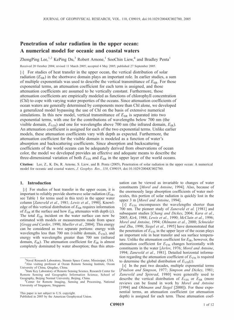
[43] The above compared T(z) values are for a fewdiscrete depths. To reveal the vertical details of T(z) in thesubsurface layer, Figure 8 presents examples of T(z) of top10 m for four commonly observed Chl values in the field.Figure 8 also shows T(z) from the standard data set. Clearly,since Morel and Antoine [1994] did not try to resolve thedetails of T(z) within the top 1 m, larger errors are found fornear-surface T(z) in the MA94 model, as pointed out byMorel and Antoine [1994]. The models of Ohlmann andSiegel [2000] and this study tried to resolve the details ofnear-surface T(z). In addition, since the attenuation in theinfrared domain is dominated by that of pure water, theresults between T(z) from OS00 and T(z) from this studyshow good agreement for the near-surface layer. Note thatfor z < 1 m, changes of water constituents have only minoreffects on T(z).

7. Discussion

[44] The T(z) values from the IOP-based model used onlyabsorption and backscattering coefficients at 490 nm; opti-cal properties at other wavelengths were ignored. The robustresults from the IOP-based model (see Figures 7 and 8)suggest that knowing the absorption and backscatteringcoefficient at 490 nm is adequate for estimation of thevertical transmittance of EVIS and ESR, as implied in earlierstudies [Barnard et al., 1999; Zaneveld et al., 1993]. This issomewhat surprising, because for studies such as the esti-mation of primary production detailed spectral informationis important [Sathyendranath et al., 1989a]. The reason forthis relaxed requirement in spectral information is that thefocus of this study is the spectrally integrated solar radiationthat is available for water heating. There could be quitedifferent absorption coefficients at 350 or 410 nm for thesame absorption coefficient at 490 nm [Lee et al., 2005b],and these differences will result in different irradiance forthose wavelengths at a specific depth. These irradiances,however, are only a small portion of the total solar radiation,and the decrease of irradiance at one wavelength may becompensated by an increase at another wavelength at thatdepth, so the sum of the irradiance of all wavelengths(which gives EVIS and ESR) may not vary much. Such ascenario is not true for depths below the euphotic zonewhere irradiance is eventually concentrated to a narrowband; but the contribution of solar radiation at such aspectral band and at such depths is small compared to theabsorbed solar energy in the upper water column.[45] The results presented here show significant improve-

ments in modeling of the vertical distribution of EVIS andESR in the upper ocean by utilization of IOPs. Such anapproach is adequate for satellite remote sensing of oceancolor and in environments where water’s optical propertiesare well measured. However, if Chl value is the onlyavailable parameter for a water environment, since thereare wide uncertainties in estimating its IOPs, we expect nosignificant difference in estimated T(z) from either IOP-based model or MA94 or OS00. It is recognized that theaccuracy of IOPs (a(490), for instance) derived from oceancolor to the best can be within �10% [Lee et al., 2002].This error will be propagated to the calculated K̂VIS(z) andthen TVIS(z). However, since K̂VIS(z) is a spectrally averagedvalue with a big portion determined by the large absorption


9 of 12

C09019

coefficients of aw(l) in the red wavelengths, only a fractionof errors in IOPs will be transferred to K̂VIS(z).[46] It is necessary to point out that the model developed

here has primarily demonstrated the strategy, concept, andadvantages of modeling the vertical transmittance of EVIS

and ESR using inherent optical properties. The work herepresented a model with the major variables such as IOPsand Sun angle incorporated, and the model is for clear-skyconditions with marine aerosols and a well-mixed surfacelayer [Mueller and Lange, 1989]. When the sky is cloudy,reduction of the total downwelling irradiance and the ratioof the visible portion (FVIS) need to be adjusted accordingly[Behrenfeld and Falkowski, 1997; Ohlmann and Siegel,2000]. However, a recent study [Bartlett et al., 1998]pointed out that clouds have only a small spectral effecton surface EVIS, which suggests that model parametersdeveloped in this study could be applicable to cloudyconditions, though a slight adjustment for qa (or subsurfacesolar zenith angle as in work by Sathyendranath and Platt[1988]) is necessary. Similarly, when the subsurface lightfield is more diffuse as a result of capillary waves [Zaneveldet al., 2001], an effective qa might also be required.However, the effects of slightly incorrect qa on the attenu-ation of EVIS are much smaller than that of incorrectabsorption and backscattering coefficients.[47] One should take caution when applying the newly

developed model to depths that are below the well-mixed

surface layer, especially if the optical properties at thosedepths are significantly different from those in the mixedlayer. For such conditions, the evaluation of downwellingirradiance at those depths will be changed, and the proper-ties retrieved from observed ocean color might also beaffected [Gordon and Clark, 1980; Sathyendranath andPlatt, 1989; Zaneveld et al., 1998]. A critical hurdle inremote sensing is the lack of instantaneous knowledge ofthe vertical distribution of the optical properties when asatellite sensor makes measurements. Historical data mayprovide a general guidance about the vertical distributions,but those measurements are insufficient and the verticaldistributions vary spatially and temporally. A method toadequately provide the details of the vertical distribution ofthe optical or biogeochemical properties of a water body isneeded. Combining measurements from satellite sensorswith outputs from dynamic oceanography models [Chai etal., 2002; McGillicuddy et al., 1995] may provide usefulalternatives to overcome the limitations of significantlystratified upper water column.

8. Conclusions

[48] In this study, an innovative model is developed fordescribing the vertical transmittance of solar radiation in theupper layer of the oceans. Similar to Morel and Antoine[1994], our study explicitly partitioned the solar radiation

Figure 8. Examples of T(z) for the top 10 m, with T(z) calculated by three models and from the standarddata set. Values of Chl, a(490), and bb(490) are provided in the insets.


10 of 12

C09019

into two portions: one for the visible domain (EVIS, 350–700 nm), and the other for the infrared domain (EIR, 700–2500 nm). For the two portions, two exponential functionsare used separately to describe their vertical transmittance.For each exponential term, an attenuation coefficient isassigned. For EIR, its attenuation coefficient (K̂IR(z)) ismodeled as a function of z and solar zenith angle. For EVIS,its attenuation coefficient (K̂VIS(z)) is modeled as a functionof depth, solar zenith angle, and water’s optical properties,after extensive numerical simulations using HydroLight.[49] Compared with earlier Chl-based models, the model

developed here has fewer empirical parameters and providesrobust and stable results in describing the vertical distribu-tion of the visible portion or the full spectrum of solarradiation in the subsurface layer. Since the model requiresa(490) and bb(490) as inputs, accurate retrieval of these twooptical properties from satellite observations of ocean coloris required. When these properties are available for worldoceans, the model can be used to provide efficient evalua-tion of EVIS(z) and ESR(z) in the well mixed upper watercolumn, which in turn can be incorporated into physicalmodels to study heat transfer [e.g., Kara et al., 2005]. Also,after consideration of the average cosine [Sathyendranathand Platt, 1988], EVIS(z) can be easily converted to photo-synthetic available radiation (PAR) and incorporated intomodels for estimating primary production of the watercolumn. In addition, the K̂VIS(z) model provides an easyand reliable tool to predict the light level at desired depthsfrom satellite IOPs, needed to plan the C14 incubation for insitu measurements of primary production [Barnard et al.,1999].

[50] Acknowledgments. Support for this study was provided by theOffice of Naval Research (P.E. 61153N and N0001405WX20623). Theauthors thank Robert F. Chen for assistance in MODTRAN calculation andHeather Melton Penta for editorial contribution, and the authors are verygrateful to Curtis Mobley for providing HydroLight code and assistance.Comments and suggestions from two reviewers are greatly appreciated.

ReferencesBarnard, A. H., J. R. V. Zaneveld, W. S. Pegau, J. L. Mueller, H. Maske,R. Lara-Lara, S. Alvarez-Borrego, R. Cervantes-Duarte, and E. Valdez-Holguin (1999), The determination of PAR levels from absorption coef-ficient profiles at 490 nm, Cienc. Mar., 25(4), 487–507.

Bartlett, J. S., A. M. Ciotti, R. F. Davis, and J. J. Cullen (1998), The spectraleffects of clouds on solar irradiance, J. Geophys. Res., 103, 31,017–31,031.

Behrenfeld, M. J., and P. G. Falkowski (1997), A consumer’s guide tophytoplankton primary productivity models, Limnol. Oceanogr., 42,1479–1491.

Berwald, J., D. Stramski, C. D. Mobley, and D. A. Kiefer (1995), Influ-ences of absorption and scattering on vertical changes in the averagecosine of the underwater light field, Limnol. Oceanogr., 40, 1347–1357.

Bricaud, A., and A. Morel (1986), Light attenuation and scattering byphytoplanktonic cells: A theoretical modeling, Appl. Opt., 25, 571–580.

Bricaud, A., A. Morel, and L. Prieur (1981), Absorption by dissolvedorganic matter of the sea (yellow substance) in the UV and visible do-mains, Limnol. Oceanogr., 26, 43–53.

Bricaud, A., M. Babin, A. Morel, and H. Claustre (1995), Variability in thechlorophyll-specific absorption coefficients of natural phytoplankton:Analysis and parameterization, J. Geophys. Res., 100, 13,321–13,332.

Carder, K. L., F. R. Chen, Z. P. Lee, S. K. Hawes, and D. Kamykowski(1999), Semianalytic Moderate-Resolution Imaging Spectrometer algo-rithms for chlorophyll a and absorption with bio-optical domains basedon nitrate-depletion temperatures, J. Geophys. Res., 104, 5403–5422.

Chai, F., R. C. Dugdale, T.-H. Peng, F. P. Wilkerson, and R. T. Barber(2002), One-dimensional ecosystem model of the equatorial Pacific up-welling system, part I: Model development and silicon and nitrogencycle, Deep Sea Res., Part II, 49, 2713–2745.

Chang, G. C., and T. D. Dickey (2004), Coastal ocean optical influences onsolar transmission and radiant heating rate, J. Geophys. Res., 109,C01020, doi:10.1029/2003JC001821.

Gordon, H. R. (1989), Can the Lambert-Beer law be applied to the diffuseattenuation coefficient of ocean water?, Limnol. Oceanogr., 34, 1389–1409.

Gordon, H. R., and D. K. Clark (1980), Remote sensing optical propertiesof a stratified ocean: An improved interpretation, Appl. Opt., 19, 3428–3430.

Gordon, H. R., and A. Morel (1983), Remote Assessment of Ocean Colorfor Interpretation of Satellite Visible Imagery: A Review, 44 pp., Springer,New York.

Gordon, H. R., O. B. Brown, and M. M. Jacobs (1975), Computed relation-ship between the inherent and apparent optical properties of a flat homo-geneous ocean, Appl. Opt., 14, 417–427.

Gordon, H. R., R. C. Smith, and J. R. V. Zaneveld (1980), Introduction toocean optics, in Proc. SPIE Soc. Opt. Eng., 208, 1–43.

Gregg, W. W., and K. L. Carder (1990), A simple spectral solar irradiancemodel for cloudless maritime atmospheres, Limnol. Oceanogr., 35,1657–1675.

Hoge, F. E., and P. E. Lyon (1996), Satellite retrieval of inherent opticalproperties by linear matrix inversion of oceanic radiance models: Ananalysis of model and radiance measurement errors, J. Geophys. Res.,101, 16,631–16,648.

International Ocean-Colour Coordinating Group (2000), Remote sensing ofocean colour in coastal, and other optically-complex, waters, Rep. 3,edited by S. Sathyendranath, 140 pp., Dartmouth, Nova Scotia, Canada.

Jerlov, N. G. (1976), Marine Optics, Elsevier, New York.Kara, A. B., A. J. Wallcraft, and H. E. Hurlburt (2005), Sea surface tem-perature sensitivity to water turbidity from simulations of the turbid BlackSea using HYCOM, J. Phys. Oceanogr., 35, 33–54.

Kirk, J. T. O. (1988), Solar heating of water bodies as influenced by theirinherent optical properties, J. Geophys. Res., 93, 10,897–10,908.

Kirk, J. T. O. (1991), Volume scattering function, average cosines, and theunderwater light field, Limnol. Oceanogr., 36, 455–467.

Kirk, J. T. O. (1994), Light and Photosynthesis in Aquatic Ecosystems,Cambridge Univ. Press, New York.

Lee, Z. P., K. L. Carder, C. D. Mobley, R. G. Steward, and J. S. Patch(1998), Hyperspectral remote sensing for shallow waters. 1. A semiana-lytical model, Appl. Opt., 37, 6329–6338.

Lee, Z. P., K. L. Carder, and R. Arnone (2002), Deriving inherent opticalproperties from water color: A multi-band quasi-analytical algorithm foroptically deep waters, Appl. Opt., 41, 5755–5772.

Lee, Z. P., K. P. Du, and R. Arnone (2005a), A model for the diffuseattenuation coefficient of downwelling irradiance, J. Geophys. Res.,110, C02016, doi:10.1029/2004JC002275.

Lee, Z. P., W. J. Rhea, R. Arnone, and W. Goode (2005b), Absorptioncoefficients of marine waters: Expanding multi-band informationto hyperspectral data, IEEE Trans. Geosci. Remote Sens., 43(1), 118–124.

Lewis, M. R., M. Carr, G. Feldman, W. Esaias, and C. McMclain (1990),Influence of penetrating solar radiation on the heat budget of theequatorial Pacific Ocean, Nature, 347, 543–545.

Liu, C.-C., R. Miller, K. L. Carder, and Z. P. Lee (2002), Estimating theunderwater light field from remote sensing, in Ocean Optics XVI [CD-ROM], edited by S. Ackleson, Off. of Naval Res. Arlington, Va.

Loisel, H., D. Stramski, B. G. Mitchell, F. Fell, V. Fournier-Sicre,B. Lemasle, and M. Babin (2001), Comparison of the ocean inherentoptical properties obtained from measurements and inverse modeling,Appl. Opt., 40, 2384–2397.

Lyon, P. E., F. E. Hoge, C. W. Wright, R. N. Swift, and J. K. Yungel (2004),Chlorophyll biomass in the global oceans: Satellite retrieval using inher-ent optical properties, Appl. Opt., 43, 5886–5892.

McClain, C., K. Arrigo, K.-S. Tai, and D. Turk (1996), Observations andsimulations of physical and biological process at ocean weather station P,1951–1980, J. Geophys. Res., 101, 3697–3713.

McGillicuddy, D. J., J. J. McCarthy, and A. R. Robinson (1995), Coupledphysical and biological modeling of the spring bloom in the NorthAtlantic I: Model formulation and one dimensional bloom processes,Deep Sea Res., Part I, 42, 1313–1357.

Mobley, C. D. (1994), Light and Water: Radiative Transfer in NaturalWaters, Elsevier, New York.

Mobley, C. D. (1995), Hydrolight 3.0 users’ guide, SRI Int., Menlo Park,Calif.

Mobley, C. D., B. Gentili, H. R. Gordon, Z. Jin, G. W. Kattawar, A. Morel,P. Reinersman, K. Stamnes, and R. H. Stavn (1993), Comparison ofnumerical models for computing underwater light fields, Appl. Opt.,32, 7484–7504.

Mobley, C. D., L. K. Sundman, and E. Boss (2002), Phase function effectson oceanic light fields, Appl. Opt., 41, 1035–1050.


11 of 12

C09019

Morel, A. (1974), Optical properties of pure water and pure sea water, inOptical Aspects of Oceanography, edited by N. G. Jerlov and E. S.Nielsen, pp. 1–24, Elsevier, New York.

Morel, A. (1978), Available, usable, and stored radiant energy in relation tomarine photosynthesis, Deep Sea Res., 25, 673–688.

Morel, A. (1988), Optical modeling of the upper ocean in relation to itsbiogenous matter content (case I waters), J. Geophys. Res., 93, 10,749–10,768.

Morel, A., and D. Antoine (1994), Heating rate within the upper ocean inrelation to its bio-optical state, J. Phys. Oceanogr., 24, 1652–1665.

Morel, A., and B. Gentili (1991), Diffuse reflectance of oceanic waters:Its dependence on Sun angle as influenced by the molecular scatteringcontribution, Appl. Opt., 30, 4427–4438.

Morel, A., and B. Gentili (1993), Diffuse reflectance of oceanic waters. II.Bidirectional aspects, Appl. Opt., 32, 6864–6879.

Morel, A., and B. Gentili (2004), Radiation transport within oceanic (case 1)water, J. Geophys. Res., 109, C06008, doi:10.1029/2003JC002259.

Morel, A., and H. Loisel (1998), Apparent optical properties of oceanicwater: Dependence on the molecular scattering contribution, Appl. Opt.,37, 4765–4776.

Morel, A., and S. Maritorena (2001), Bio-optical properties of oceanicwaters: A reappraisal, J. Geophys. Res., 106, 7163–7180.

Morel, A., and L. Prieur (1977), Analysis of variations in ocean color,Limnol. Oceanogr., 22, 709–722.

Mueller, J. L., and R. E. Lange (1989), Bio-optical provinces of the north-east Pacific Ocean: A provisional analysis, Limnol. Oceanogr., 34,1572–1586.

Mueller, R. W., et al. (2004), Rethinking satellite-based solar irradiancemodelling: The SOLIS clear-sky module, Remote Sens. Environ., 91,160–174.

Ohlmann, J. C., and D. Siegel (2000), Ocean radiant heating. Part II:Parameterizing solar radiation transmission through the upper ocean,J. Phys. Oceanogr., 30, 1849–1865.

Ohlmann, J. C., D. A. Siegel, and C. D. Mobley (2000), Ocean radiantheating. part I: Optical influences, J. Phys. Oceanogr., 30, 1833–1848.

Paulson, C. A., and J. J. Simpson (1977), Irradiance measurements in theupper ocean, J. Phys. Oceanogr., 7, 953–956.

Paulson, C. A., and J. J. Simpson (1981), The temperature difference acrossthe cool skin of the ocean, J. Geophys. Res., 86, 11,044–11,054.

Pegau, W. S., and J. R. V. Zaneveld (1993), Temperature-dependentabsorption of water in the red and near-infrared portions of the spectrum,Limnol. Oceanogr., 38, 188–192.

Pegau, W. S., D. Gray, and J. R. V. Zaneveld (1997), Absorption andattenuation of visible and near-infrared light in water: Dependence ontemperature and salinity, Appl. Opt., 36, 6035–6046.

Pope, R., and E. Fry (1997), Absorption spectrum (380–700 nm) of purewaters: II. Integrating cavity measurements, Appl. Opt., 36, 8710–8723.

Preisendorfer, R. W. (1976), Hydrologic Optics, vol. 1, Introduction, Natl.Tech. Inf. Serv., Springfield, Va.

Sathyendranath, S., and T. Platt (1988), The spectral irradiance field at thesurface and in the interior of the ocean: A model for applications inoceanography and remote sensing, J. Geophys. Res., 93, 9270–9280.

Sathyendranath, S., and T. Platt (1989), Remote sensing of oceanchlorophyll: Consequence of nonuniform pigment profile, Appl. Opt.,28, 490–495.

Sathyendranath, S., T. Platt, C. M. Caverhill, R. E. Warnock, and M. R.Lewis (1989a), Remote sensing of oceanic primary production: Compu-tations using a spectral model, Deep Sea Res., Part A, 36, 431–453.

Sathyendranath, S., L. Prieur, and A. Morel (1989b), A three-componentmodel of ocean colour and its application to remote sensing of phyto-plankton pigments in coastal waters, Int. J. Remote Sens., 10, 1373–1394.

Sathyendranath, S., G. Cota, V. Stuart, M. Maass, and T. Platt (2001),Remote sensing of phytoplankton pigments: A comparison of empiricaland theoretical approaches, Int. J. Remote Sens., 22, 249–273.

Schneider, E. K., and Z. Zhu (1998), Sensitivity of the simulated annualcycle of sea surface temperature in the Equatorial Pacific to sunlightpenetration, J. Clim., 11, 1932–1950.

Siegel, D., J. C. Ohlmann, L. Washburn, R. R. Bidigare, C. T. Nosse,E. Fields, and Y. Zhou (1995), Solar radiation, phytoplankton pigmentsand radiant heating of the equatorial Pacific warm pool, J. Geophys. Res.,100, 4885–4891.

Simpson, J. J., and T. D. Dickey (1981), Alternative parameterizations ofdownward irradiance and their dynamic significance, J. Phys. Oceanogr.,11, 876–882.

Smith, R. C., and K. S. Baker (1981), Optical properties of the clearestnatural waters, Appl. Opt., 20, 177–184.

Stramski, D., A. Bricaud, and A. Morel (2001), Modeling the inherentoptical properties of the ocean based on the detailed composition of theplanktonic community, Appl. Opt., 40, 2929–2945.

Zaneveld, J. R. V. (1989), An asymptotic closure theory for irradiance in thesea and its inversion to obtain the inherent optical properties, Limnol.Oceanogr., 34, 1442–1452.

Zaneveld, J. R. V., and R. W. Spinrad (1980), An arc tangent model ofirradiance in the sea, J. Geophys. Res., 85, 4919–4922.

Zaneveld, J. R. V., J. C. Kitchen, and H. Pak (1981), The influence ofoptical water type on the heating rate of a constant depth mixed layer,J. Geophys. Res., 86, 6426–6428.

Zaneveld, J. R. V., J. C. Kitchen, and J. L. Mueller (1993), Vertical structureof productivity and its vertical integration as derived from remotelysensed observations, Limnol. Oceanogr., 38, 1384–1393.

Zaneveld, J. R. V., A. H. Barnard, W. S. Pegau, and E. Boss (1998), Aninvestigation into the appropriate depth average of remotely sensedoptical parameters, in Ocean Optics XIV [CD-ROM], edited byS. Ackleson and J. Campbell, Off. of Naval Res. Arlington, Va.

Zaneveld, J. R. V., E. Boss, and P. A. Hwang (2001), The influence ofcoherent waves on the remotely sensed reflectance, Opt. Express, 9(6),260–266.

��R. Arnone, Z. Lee, and B. Penta, Naval Research Lab, Code 7333,

Stennis Space Center, MS 39529, USA. ([email protected])K. Du, State Key Laboratory of Remote Sensing Science, Research

Center for Remote Sensing and GIS, School of Geography, Beijing NormalUniversity, Beijing, 100875, China.S. Liew, Center for Remote Imaging, Sensing and Processing, National

University of Singapore, Lower Kent Ridge Road, Singapore 119260.


12 of 12

C09019

Documents

Penetration of solar radiation in the upper ocean: A