Peer-to-Peer Lenders versus Banks:Substitutes or Complements?

Huan Tang∗

ABSTRACT

This paper studies whether peer-to-peer (P2P) lending platforms operate as sub-stitutes to banks or instead complement them in consumer credit markets. I developa framework and derive testable predictions to distinguish between the two cases. Us-ing a regulatory change as an exogenous shock to bank credit supply, I find that P2Plending is a substitute to bank lending in that it serves infra-marginal bank borrowers,but also complements bank lending for small-size loans. These findings suggest thatthe credit expansion P2P lending brings about is likely to occur only among borrowerswith access to bank credit.

Keywords: peer-to-peer lending; access to credit; financial innovation.

JEL Classification: D14, E51, G2

∗HEC Paris, 1 rue de la liberation, 78350 Jouy-en-Josas, France; email: huan.tang@hec.edu. I am gratefulto Denis Gromb, Johan Hombert, and Guillaume Vuillemey for their support and guidance. I also thank thediscussant (Gerard Hoberg), the editors (Andrew Karolyi, Itay Goldstein, and Wei Jiang), Xiaoyan Zhang,and the participants at the RFS FinTech Workshop (Columbia, 2017) and Tsinghua PBC School of Financefor their helpful comments.

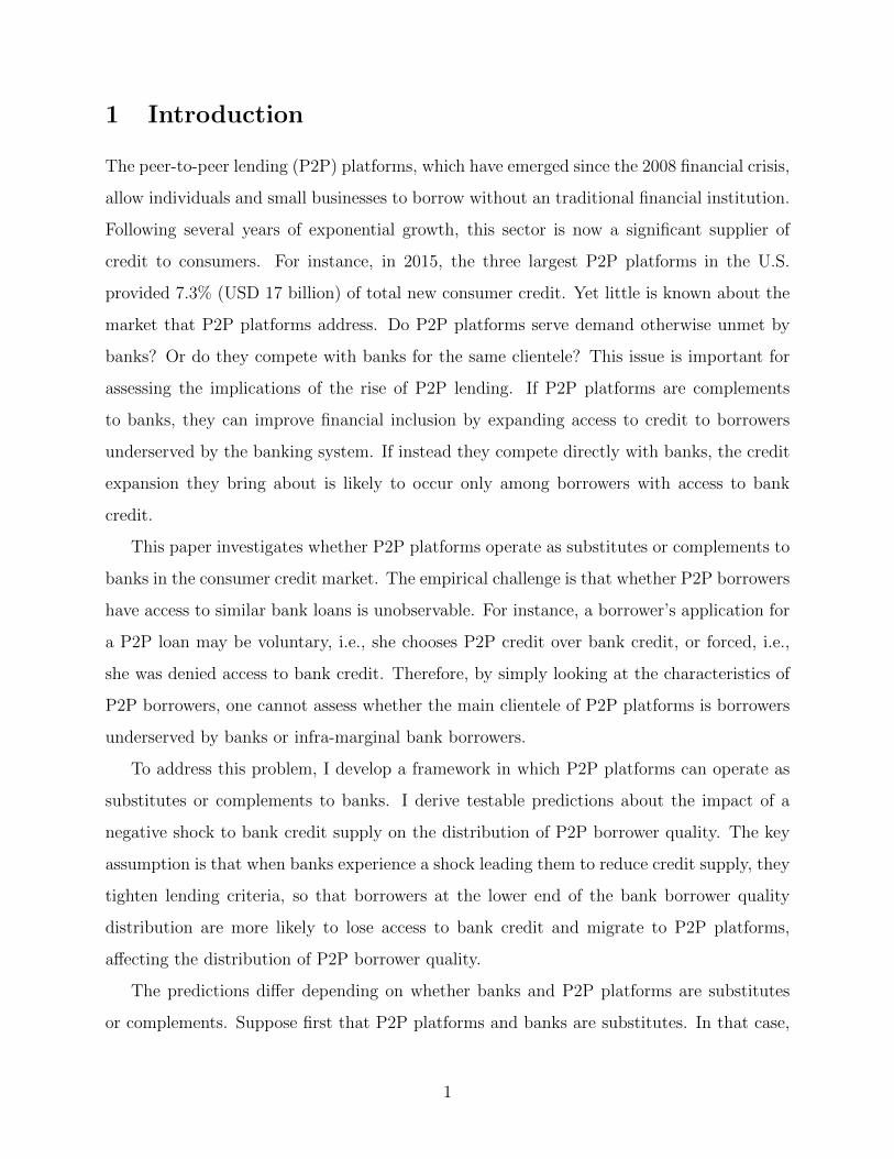
1 Introduction

The peer-to-peer lending (P2P) platforms, which have emerged since the 2008 financial crisis,

allow individuals and small businesses to borrow without an traditional financial institution.

Following several years of exponential growth, this sector is now a significant supplier of

credit to consumers. For instance, in 2015, the three largest P2P platforms in the U.S.

provided 7.3% (USD 17 billion) of total new consumer credit. Yet little is known about the

market that P2P platforms address. Do P2P platforms serve demand otherwise unmet by

banks? Or do they compete with banks for the same clientele? This issue is important for

assessing the implications of the rise of P2P lending. If P2P platforms are complements

to banks, they can improve financial inclusion by expanding access to credit to borrowers

underserved by the banking system. If instead they compete directly with banks, the credit

expansion they bring about is likely to occur only among borrowers with access to bank

credit.

This paper investigates whether P2P platforms operate as substitutes or complements to

banks in the consumer credit market. The empirical challenge is that whether P2P borrowers

have access to similar bank loans is unobservable. For instance, a borrower’s application for

a P2P loan may be voluntary, i.e., she chooses P2P credit over bank credit, or forced, i.e.,

she was denied access to bank credit. Therefore, by simply looking at the characteristics of

P2P borrowers, one cannot assess whether the main clientele of P2P platforms is borrowers

underserved by banks or infra-marginal bank borrowers.

To address this problem, I develop a framework in which P2P platforms can operate as

substitutes or complements to banks. I derive testable predictions about the impact of a

negative shock to bank credit supply on the distribution of P2P borrower quality. The key

assumption is that when banks experience a shock leading them to reduce credit supply, they

tighten lending criteria, so that borrowers at the lower end of the bank borrower quality

distribution are more likely to lose access to bank credit and migrate to P2P platforms,

affecting the distribution of P2P borrower quality.

The predictions differ depending on whether banks and P2P platforms are substitutes

or complements. Suppose first that P2P platforms and banks are substitutes. In that case,

1

they serve the same clientele before the shock, with the same distribution of borrower quality.

Following a negative shock to bank credit supply, low-quality bank borrowers will migrate to

P2P platforms. As a result, the average P2P borrower quality should drop and the quantiles

of the distribution of P2P borrower quality shift left.

Suppose instead that P2P platforms complement banks by addressing a low-quality bor-

rower segment underserved by banks. In that case, the borrower pool of P2P platforms is

of worse quality than banks. Upon the shock to bank credit supply, the borrowers switching

from banks to P2P platforms will improve the quality of the P2P borrower pool. As a result,

the average P2P borrower quality will increase, and the quantiles of the distribution of P2P

borrower quality shift right.

To test these predictions empirically, I exploit a regulatory change that caused banks to

tighten their lending criteria. In 2010, the Financial Accounting Standards Board (FASB)

implemented a new regulation (FAS 166/167) requiring banks to consolidate securitized off-

balance sheet assets onto their balance sheets and include them in the risk-weighted assets

starting in 2011Q1. In aggregate, this caused banks to consolidate USD 399.9 billion of

assets, over 80% of which were revolving consumer loans.1 The change in accounting had a

large effect on banks lending through its impact on regulatory capital. Different banks were

affected differently depending on how much securitized assets qualifying for consolidation

they held off-balance sheet. Affected banks reduced small business lending and mortgage

approval rates (Dou 2016; Dou, Ryan, and Xie 2016), and increased the average quality of

credit card loans (Tian and Zhang 2016).

I conjecture that the shock affect local credit markets differently depending on the ex-

posure of local banks to the new regulation. I identify banks as being affected if they held

off-balance sheet assets qualifying for the consolidation under FAS 166/167. Counties with

at least one affected bank are defined as affected markets, other counties forming a control

group. I then examine the change in the distribution of P2P borrower quality in affected

markets. Hence, the bank credit supply shock’s impact on the distribution of P2P borrower

quality is identified by the variation in exposure to the shock across local markets.

1See the Board of Governors of the Federal Reserve System’s “Notes on Data” of the data set “Assetsand Liabilities of Commercial Banks in the United States - H.8”, released on April 9, 2010, available at:https://www.federalreserve.gov/releases/h8/h8notes.htm.

2

I use information on asset consolidation from the annual Call Reports to identify affected

banks. In total, 59 banks have consolidated assets under FAS 166/167. The data on P2P

lending volume, loan application and borrower characteristics (FICO score, debt-to-income

ratio, employment, etc.) as well as loan characteristics is obtained from LendingClub, a large

P2P platform whose market share represents over 50% of P2P personal loans in the U.S. I

construct county-level variables using the data on 880,346 loan applications and 93,159 loan

originations during 2009-12. The final sample consists of 1,908 affected and 1,025 unaffected

markets, defined at the county level. On average, per thousand inhabitants in a county, the

number of P2P loan applications and the number of funded loans originated are 0.6 and 0.05

per year, respectively.

I start by examining the treatment effect of FAS 166/167 on P2P loan application and

origination volumes. I find that compared to the control group, affected markets experience

an increase in P2P loan applications. On average, per thousand inhabitants in the county,

0.07 more applications are made for an additional amount of USD 1,108, which represents

a 27% increase in the number of applications and a 42% increase in the dollar amount.

The results suggest that some borrowers who would otherwise have been served by banks

turned to P2P platforms. Moreover, it appears that this additional demand was partially

satisfied by P2P platforms. I find that compared to the control group, affected markets also

saw an increase in the number and dollar amount of P2P loans. On average, per thousand

inhabitants in the county, 0.016 more P2P loans were originated for an additional amount

of USD 301. Compared to the pre-shock level of origination, the number of loans increases

by 1.1 times and the dollar amount of loans increases by 1.5 times.

Second, I test the predictions regarding the shock’s impact on the distribution of P2P

borrower quality. Using FICO scores as a measure of borrower quality, I find that com-

pared to the control group, affected markets experience a left shift of all quantiles of the

distribution. These findings suggest that P2P loans are substitutes to bank loans.

Other tests on the frequency distribution of P2P borrower quality lend additional support

to this interpretation. If bank borrowers migrating to P2P platforms are of worse quality than

existing P2P borrowers, one should observe a higher frequency only in the low-FICO range of

the P2P borrower quality distribution. This is indeed what I find. The number of originations

3

increases by 1.6 times among borrowers with FICO scores below 690, which corresponds to

the 45th percentile of the pre-shock distribution of P2P borrowers. In contrast, there is no

significant change in the number of originations in the upper end of the borrower distribution.

FICO scores are a coarse measure of borrower quality, and banks often use additional

information to assess default risk. For example, the primary reasons for mortgage application

denials, as reported in the Home Mortgage Disclosure Act, include credit history, the debt-to-

income ratio and length of employment. Therefore, I construct another measure of borrower

quality combining FICO score, debt-to-income ratio, and length of employment. Specifically,

I estimate an ordered probit model taking application outcomes (rejected, qualified but

not funded, or qualified and funded) as the dependent variable and the three borrower

characteristics as explanatory variables, and summarize all the information into a single

cardinal measure, the predicted application quality.

Using the new measure in the quantile and frequency tests delivers similar results. First,

compared to the control group, the predicted borrower quality distribution in affected mar-

kets experiences a left shift of all quantiles. The average predicted quality also decreases,

although not significantly at the conventional levels. Second, the increase in the number of

originations comes from borrowers with predicted quality below the 20th percentile. The

overall number of originations among those low-quality borrowers increases by 1.3 times.

Again, these results are consistent with P2P platforms operating as substitutes to banks.

Overall, these findings suggest that P2P platforms are substitutes to banks in that they

serve the same borrower population. However, the technological advantage of P2P platforms

may allow them to operate as complements to banks in the dimension of loan size. More

specifically, due to a low fixed cost of originating loans, P2P platforms may focus on the

small loan size segment compared to banks. I thus repeat the analysis for the distribution of

loan size. I find that borrowers migrating from banks to P2P platforms apply for larger loans

than pre-existing P2P borrowers. Compared to the control group, the average loan size in

affected markets increases by 9.6% (USD 1,066) and the loan size distribution experiences

a right shift of almost all quantiles. Frequency tests show that the number of originations

quadrupled for loans larger than the 80th percentile of the pre-shock loan size distribution. In

contrast, the number of loans of smaller size does not change significantly. This is consistent

4

with P2P platforms operating as complements to banks by offering smaller loans.

To understand the implication of the expansion of P2P lending for P2P investors, I

analyze loan performance before and after the shock. Controlling for borrower characteristics,

I find that loans originated after the shock are not more likely to default or being late in

payment. Therefore, loan performance does not deteriorate after the shock.

Taken together, the evidence suggests that P2P platforms operate as substitutes to banks

by serving infra-marginal bank borrowers. The expansion of P2P lending is likely to mostly

benefit this group of borrowers. P2P credit is fungible with bank credit for borrowers who

could have been served by banks, though loans offered by P2P platforms tend to be smaller.

Much of the emerging literature on P2P lending focuses on investor behavior in relation

to borrower characteristics, e.g., appearance, disclosures, and social networks (Herzenstein,

Sonenshein, and Dholakia 2011; Michels 2012; Duarte, Siegel, and Young 2012; Lin, Prabhala,

and Viswanathan 2013; Freedman and Jin 2017). Several papers document herding by online

lenders (Kim and Viswanathan 2016; Chuprinin and Hu 2016; Zhang and Liu 2012). Another

line of research studies the information production and efficiency in P2P market through

auctions (Franks, Serrano-Velarde, and Sussman 2016), screening accuracy (Balyuk (2016)),

and the use of non-standard information (Iyer et al. 2015).

The current study is among the first to investigate P2P lending in relation to bank lend-

ing. Previous papers show mixed evidence on the type of borrowers served by P2P platforms

relative to banks. For example, Buchak et al. (2017) document complementarity between

FinTech lenders and banks in the residential lending market. They find that shadow banks,

including FinTech lenders, gain a larger share among less creditworthy borrowers. Similar

results are also found in the consumer credit market in Germany and China (De Roure, Peliz-

zon, and Tasca 2016; Liao et al. 2017). However, some opposite results have been documents

in the U.S. consumer credit market. Wolfe and Yoo (2017) provide evidence in line with P2P

platforms being substitutes to banks as small (rural) commercial banks lose lending volume

in response to P2P lending encroachment.

This study differs from the previous ones in several ways. First, I address explicitly the

issue whether P2P borrowers could have obtained bank credit by considering a shock to bank

credit supply. Second, I provide causal evidence that borrowers substitute bank credit with

5

P2P credit. Third, whereas most studies focus on the average borrower quality, I provide

precise characterization of the borrowers who migrate from banks to P2P platforms.

The rest of the paper proceeds as follows. Section 2 outlines the conceptual framework.

Sections 3 and 4 describe the institutional background of P2P lending and the data. Section 5

presents the empirical strategy. Section 6 reports main results on P2P lending volume and

borrower composition, while some additional results on P2P loan size and performance are

presented in Section 7. Finally, Section 8 concludes.

2 Conceptual Framework

To guide the empirical investigation of the P2P-bank relationship, I analyze a simple frame-

work in which P2P lenders and banks coexist. In particular, I derive predictions about the

impact of a negative shock to bank credit supply on the quantity and composition of P2P

loans.

There is a population of potential borrowers with quality γ distributed according to

certain distribution. They can borrow either from a bank or from a P2P platform. I make

two simplifying assumptions on the supply side and the demand side of the lending market.

First, bank credit supply and P2P credit supply to borrowers with quality above some

threshold γi are perfectly elastic, and the elasticities are zero to borrowers with quality

below γi, for i P tbank, P2P u. Second, for any level of borrower quality, a fraction α P r0, 1s

of borrowers choose to borrow from P2P platforms if they can obtain credit from either

banks or P2P platforms.

To streamline the discussion, I first consider two polar cases in which P2P platforms are

either perfect substitutes or perfect complements to banks, and then discuss intermediate

cases. Each case is characterized by the value of three parameters: γbank, γP2P and α.

2.1 Perfect substitutes

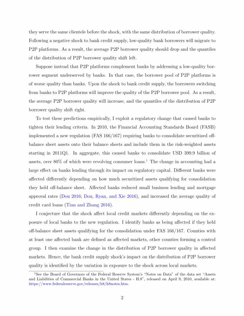
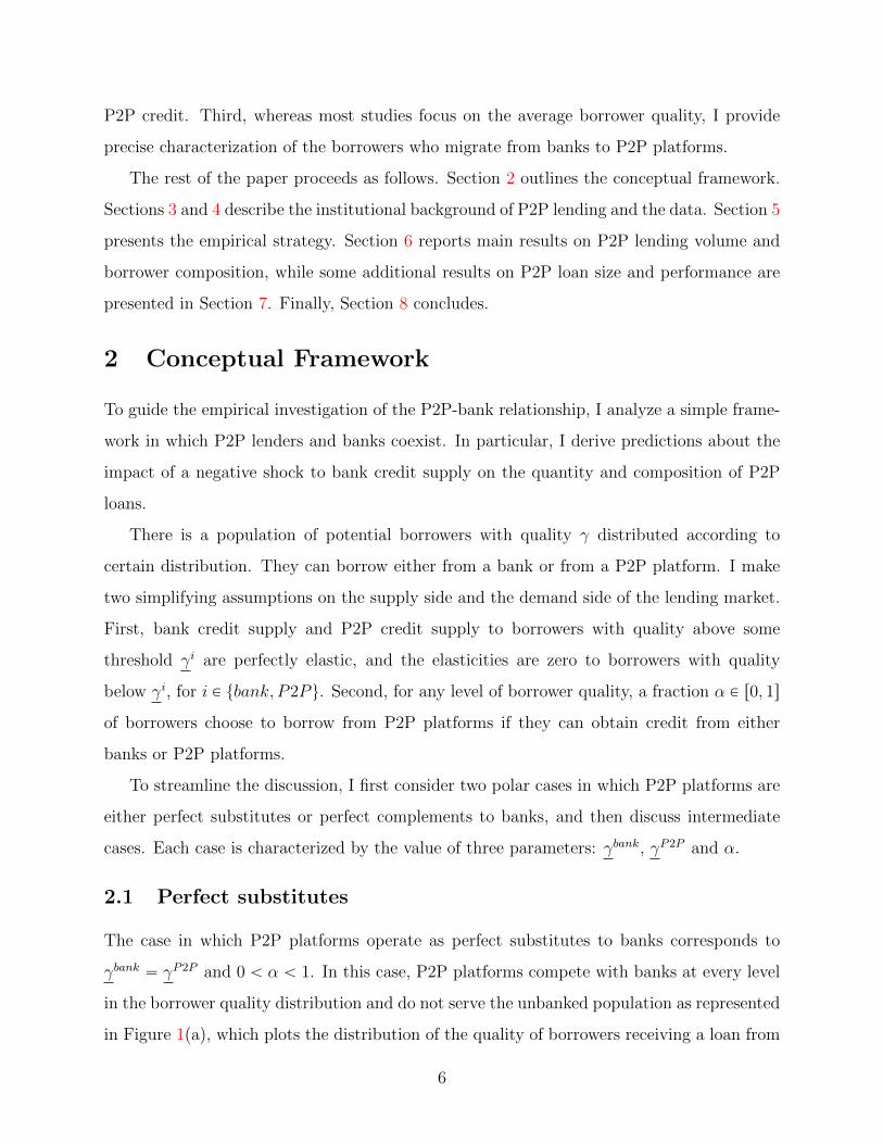
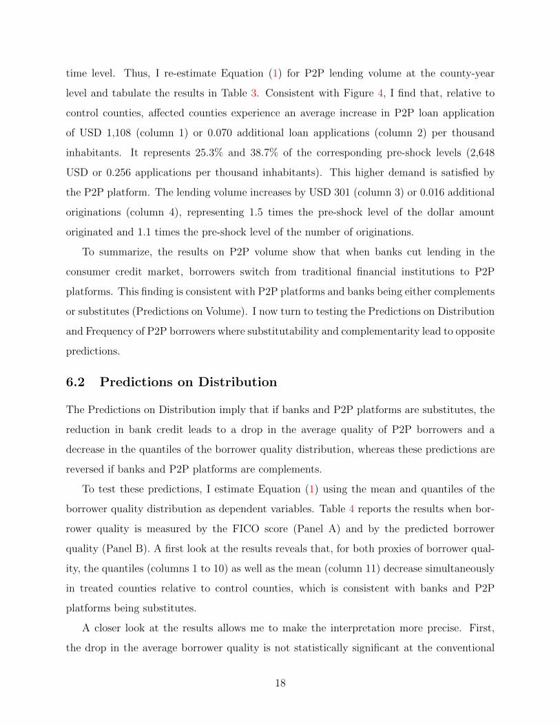
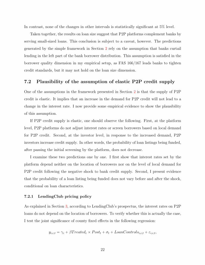
The case in which P2P platforms operate as perfect substitutes to banks corresponds to

γbank “ γP2P and 0 ă α ă 1. In this case, P2P platforms compete with banks at every level

in the borrower quality distribution and do not serve the unbanked population as represented

in Figure 1(a), which plots the distribution of the quality of borrowers receiving a loan from

6

either a bank or a P2P platform (blue curve) and the part of this distribution served by P2P

platforms (red curve).

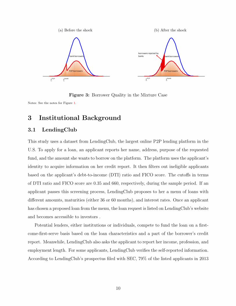
(a) Before the shock (b) After the shock

P2P borrowers

bankborrowers

𝛾"#$% = 𝛾'('

borrowersrejectedbybanks

bankborrowers

𝛾"#" 𝛾$%&'

Figure 1: Borrower Quality Distribution: Perfect Substitutes

Notes: This figure shows the change in the P2P borrower quality distribution when banks tighten their lending criteria. The

line at the top depicts the aggregate distribution of borrower quality; the area in orange represents the borrowers served by P2P

platforms, while the area between the blue curve and the red curve are the borrowers served by banks. Panel (a) shows the initial

distribution of P2P borrowers in the case of perfect substitutability (i.e., P2P platforms and banks serve the same population).

Panel (b) shows the distributions after banks tighten their lending criteria; the borrowers in the red area switch to P2P platforms.

Consider now that the effect of a tightening of banks’ lending criteria, i.e., an increase in

γbank, as illustrated in Figure 1(b). Borrowers with quality between γP2P and γbank previously

borrowing from banks now obtain credit from P2P platforms. The quality of the borrowers

migrating from banks to P2P platforms is at the low end of the pre-shock distribution of P2P

borrower quality. It implies that the distribution of P2P borrower quality shifts to the left

after the shock. More precisely, all the quantiles of the P2P borrower quality distribution

decreases, while the increase in P2P lending volume is concentrated at the low end of the

borrower quality distribution. To summarize:

Predictions from Substitutability: If P2P platforms and banks are perfect substi-

tutes, a tightening of banks’ lending criteria leads to the following predictions about P2P

borrowers:

1. Volume: a higher P2P lending volume;

2. Distribution: a lower average P2P borrower quality and lower quantiles of the P2P

borrower quality distribution;

7

3. Frequency: a higher P2P lending volume only in the low end of the pre-shock borrower

quality distribution.

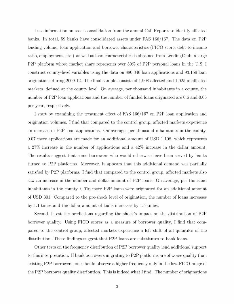
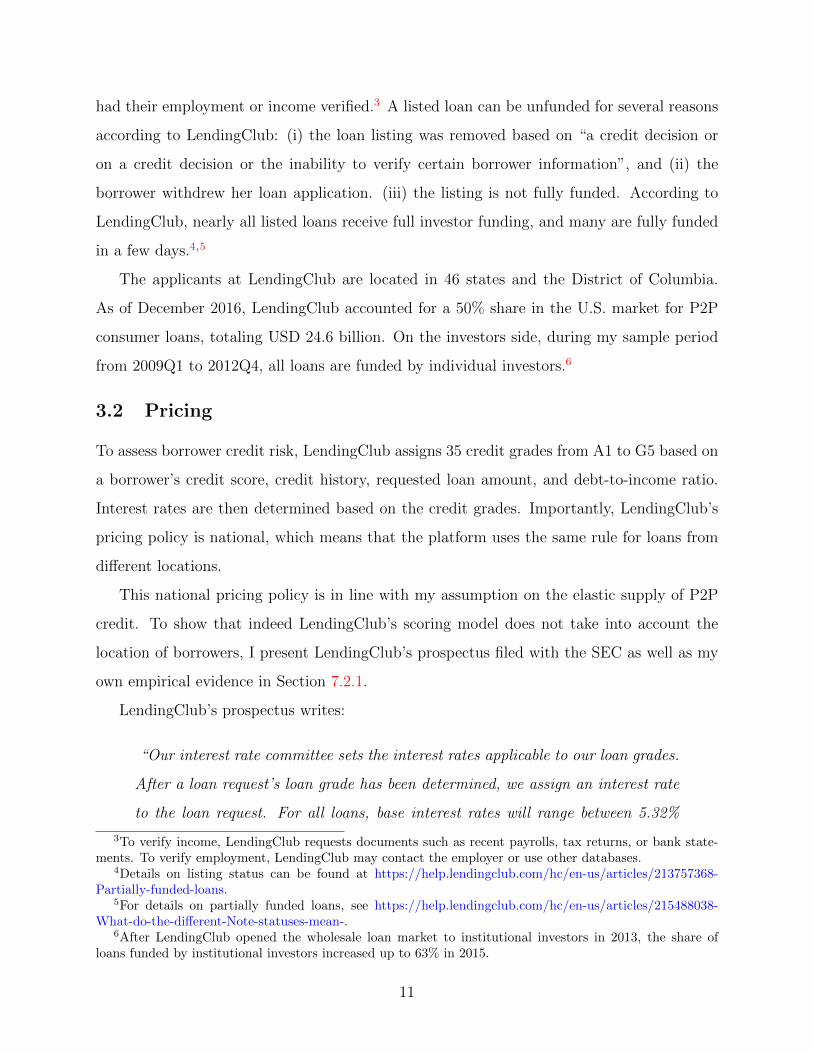
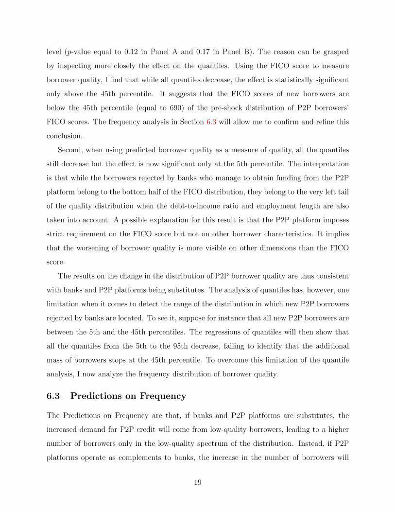
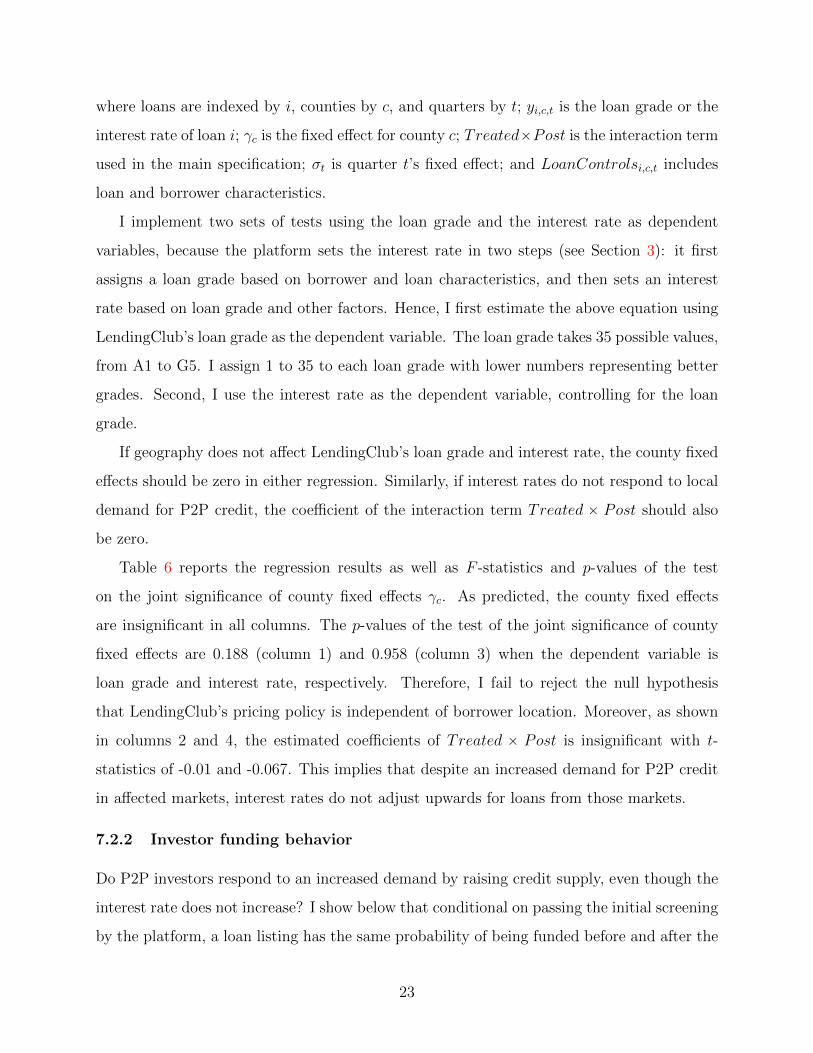
2.2 Perfect complements

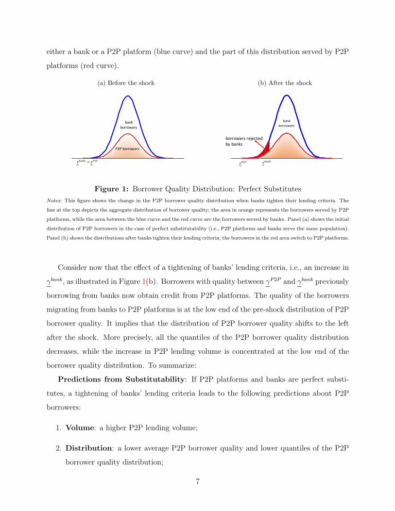
P2P platforms are perfect complements to banks corresponds to γP2P ă γbank and α “ 0. In

this case, P2P platforms and banks serve two non-overlapping segments of the market, with

banks taking the high-quality borrowers and P2P platforms lending to individuals unable to

obtain credit from banks, as represented in (Figure 2(a)).

(a) Before the shock (b) After the shock

P2P borrowers

bankborrowers

𝛾"#" 𝛾$%&'

borrowersrejectedbybanks

bankborrowers

𝛾"#$%𝛾&'&

Figure 2: Borrower Quality Distribution: Perfect Complements

Notes: See the notes for Figure 1.

Again, consider a tightening of banks’ lending criteria: γbank increases, as illustrated in

(Figure 2(b)). Borrowers of quality between the pre-shock and post-shock values of γbank

are denied access to bank credit and now borrow from P2P platforms. The quality of these

new P2P borrowers is at the high end of the pre-shock distribution of P2P borrower quality.

Therefore, the distribution of P2P borrower quality shifts to the right after the shock: all

quantiles shift right. In addition, the increase in P2P lending volume is concentrated at the

high end of the borrower quality distribution. To summarize:

Predictions from Complementarity: If P2P platforms and banks are perfect com-

plements, a reduction in bank credit supply leads to the following predictions about P2P

borrowers:

1. Volume: a higher P2P lending volume;

8

2. Distribution: a higher average P2P borrower quality and higher quantiles of the P2P

borrower quality distribution;

3. Frequency: a higher P2P lending volume only in the high end of the pre-shock bor-

rower quality distribution.

Comparing the predictions from substitutability with those from complementarity, one

can notice that while the effect of the shock on P2P lending volume is the same whether P2P

platforms substitute or complement banks, the effects on the distribution and frequency of

P2P borrower quality are opposite. These opposite predictions will allow me to distinguish

between the two cases in the empirical analysis.

As all the predictions are categorized into three groups (volume, distribution, and fre-

quency), in the following, I use “Predictions on Volume” to refer to the predictions on

volume from both substitutability and complementarity. “Predictions on Distribution” and

“Predictions on Frequency” are similarly defined.

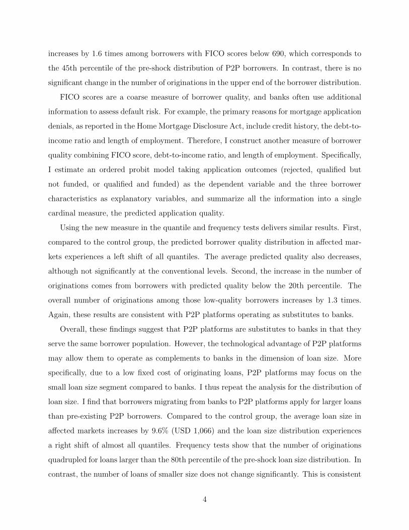
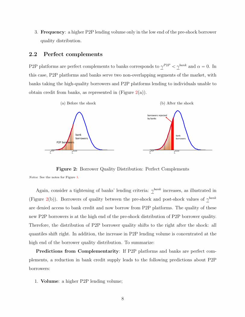
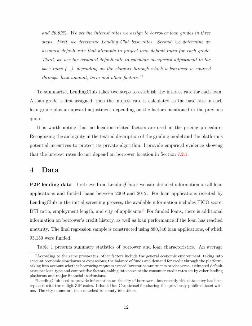
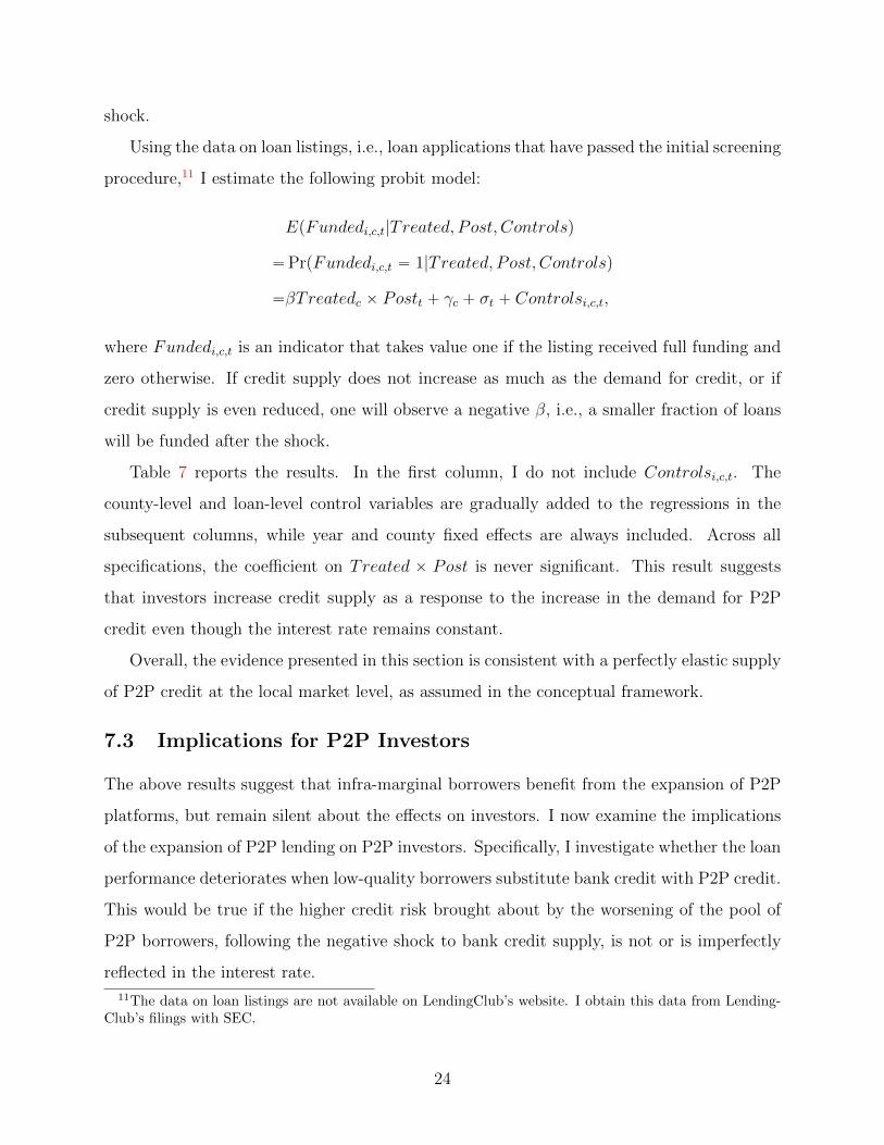
2.3 An intermediate case

My simple framework can also accommodate intermediate cases between perfect substi-

tutability and perfect complementarity of banks and P2P platforms. For instance, P2P

platforms may be substitutes to bank in the range of borrower quality served by banks while

also complementing banks by lending to borrowers unserved by banks, i.e., γP2P ă γbank and

0 ă α ă 1, as represented in Figure 3(a). In this case, a tightening of banks’ lending criteria

will lead to an increase in P2P lending volume in the middle part of the P2P borrower quality

distribution, as illustrated in Figure 3(b). Thus, analyzing changes in the frequency distribu-

tion of P2P borrower quality induced by the shock will also allow me to detect intermediate

cases between perfect substitutability and perfect complementarity.2 More specifically, the

the tightening of lending criteria leads to a higher P2P lending volume in the middle of the

distribution depending on the degree of substitution and complementarity.

2Another possibility not considered here is that P2P platforms cherry pick the highest-quality borrowerswhile banks lend to the rest of the population. In this case, a tightening of banks’ lending criteria wouldhave no effect on P2P lending volume, which I reject in the empirical analysis (see Section 6.1).

9

(a) Before the shock (b) After the shock

P2P borrowers

bank borrowers

𝛾"#" 𝛾$%&'

P2P borrowers

bank borrowersborrowersrejectedbybanks

𝛾"#" 𝛾$%&'

Figure 3: Borrower Quality in the Mixture Case

Notes: See the notes for Figure 1.

3 Institutional Background

3.1 LendingClub

This study uses a dataset from LendingClub, the largest online P2P lending platform in the

U.S. To apply for a loan, an applicant reports her name, address, purpose of the requested

fund, and the amount she wants to borrow on the platform. The platform uses the applicant’s

identity to acquire information on her credit report. It then filters out ineligible applicants

based on the applicant’s debt-to-income (DTI) ratio and FICO score. The cutoffs in terms

of DTI ratio and FICO score are 0.35 and 660, respectively, during the sample period. If an

applicant passes this screening process, LendingClub proposes to her a menu of loans with

different amounts, maturities (either 36 or 60 months), and interest rates. Once an applicant

has chosen a proposed loan from the menu, the loan request is listed on LendingClub’s website

and becomes accessible to investors .

Potential lenders, either institutions or individuals, compete to fund the loan on a first-

come-first-serve basis based on the loan characteristics and a part of the borrower’s credit

report. Meanwhile, LendingClub also asks the applicant to report her income, profession, and

employment length. For some applicants, LendingClub verifies the self-reported information.

According to LendingClub’s prospectus filed with SEC, 79% of the listed applicants in 2013

10

had their employment or income verified.3 A listed loan can be unfunded for several reasons

according to LendingClub: (i) the loan listing was removed based on “a credit decision or

on a credit decision or the inability to verify certain borrower information”, and (ii) the

borrower withdrew her loan application. (iii) the listing is not fully funded. According to

LendingClub, nearly all listed loans receive full investor funding, and many are fully funded

in a few days.4,5

The applicants at LendingClub are located in 46 states and the District of Columbia.

As of December 2016, LendingClub accounted for a 50% share in the U.S. market for P2P

consumer loans, totaling USD 24.6 billion. On the investors side, during my sample period

from 2009Q1 to 2012Q4, all loans are funded by individual investors.6

3.2 Pricing

To assess borrower credit risk, LendingClub assigns 35 credit grades from A1 to G5 based on

a borrower’s credit score, credit history, requested loan amount, and debt-to-income ratio.

Interest rates are then determined based on the credit grades. Importantly, LendingClub’s

pricing policy is national, which means that the platform uses the same rule for loans from

different locations.

This national pricing policy is in line with my assumption on the elastic supply of P2P

credit. To show that indeed LendingClub’s scoring model does not take into account the

location of borrowers, I present LendingClub’s prospectus filed with the SEC as well as my

own empirical evidence in Section 7.2.1.

LendingClub’s prospectus writes:

“Our interest rate committee sets the interest rates applicable to our loan grades.

After a loan request’s loan grade has been determined, we assign an interest rate

to the loan request. For all loans, base interest rates will range between 5.32%

3To verify income, LendingClub requests documents such as recent payrolls, tax returns, or bank state-ments. To verify employment, LendingClub may contact the employer or use other databases.

4Details on listing status can be found at https://help.lendingclub.com/hc/en-us/articles/213757368-Partially-funded-loans.

5For details on partially funded loans, see https://help.lendingclub.com/hc/en-us/articles/215488038-What-do-the-different-Note-statuses-mean-.

6After LendingClub opened the wholesale loan market to institutional investors in 2013, the share ofloans funded by institutional investors increased up to 63% in 2015.

11

and 30.99%. We set the interest rates we assign to borrower loan grades in three

steps. First, we determine Lending Club base rates. Second, we determine an

assumed default rate that attempts to project loan default rates for each grade.

Third, we use the assumed default rate to calculate an upward adjustment to the

base rates (...) depending on the channel through which a borrower is sourced

through, loan amount, term and other factors.”7

To summarize, LendingClub takes two steps to establish the interest rate for each loan.

A loan grade is first assigned, then the interest rate is calculated as the base rate in each

loan grade plus an upward adjustment depending on the factors mentioned in the previous

quote.

It is worth noting that no location-related factors are used in the pricing procedure.

Recognizing the ambiguity in the textual description of the grading model and the platform’s

potential incentives to protect its private algorithm, I provide empirical evidence showing

that the interest rates do not depend on borrower location in Section 7.2.1.

4 Data

P2P lending data I retrieve from LendingClub’s website detailed information on all loan

applications and funded loans between 2009 and 2012. For loan applications rejected by

LendingClub in the initial screening process, the available information includes FICO score,

DTI ratio, employment length, and city of applicants.8 For funded loans, there is additional

information on borrower’s credit history, as well as loan performance if the loan has reached

maturity. The final regression sample is constructed using 880,346 loan applications, of which

93,159 were funded.

Table 1 presents summary statistics of borrower and loan characteristics. An average

7According to the same prospectus, other factors include the general economic environment, taking intoaccount economic slowdowns or expansions; the balance of funds and demand for credit through the platform,taking into account whether borrowing requests exceed investor commitments or vice versa; estimated defaultrates per loan type and competitive factors, taking into account the consumer credit rates set by other lendingplatforms and major financial institutions.

8LendingClub used to provide information on the city of borrowers, but recently this data entry has beenreplaced with three-digit ZIP codes. I thank Don Carmichael for sharing this previously-public dataset withme. The city names are then matched to county identifiers.

12

borrower has a FICO score of 711, a DTI ratio of 0.147, around 6 years of working experience,

and applies for a loan of USD 13,224. The average interest rate is 13.3%, with the minimum

being 5.4% and the maximum being 24.9%.

Bank data Banks that consolidate securitized assets under FAS 166/167 report the size of

consolidated Variable Interest Entities (VIEs) in Schedule RC-V of the Call Reports starting

in 2011Q1. I use the annual Call Reports to identify banks that consolidate securitized

assets under FAS 166/167, and the Summary of Deposits to identify counties with presence

of branches from those banks.

I also use use the Summary of Deposits to construct variables of the banking market

structure at the county level: HHI, share of small banks, share of national banks, and the

geographical diversity of local banks.

5 Empirical Strategy

In this section, I describe the main empirical strategy for testing the hypotheses generated

by the conceptual framework in Section 2.

5.1 Identification strategy

Natural experiments in which banks cut lending for reasons unrelated to credit demand are

rare. I circumvent this difficulty by exploiting an arguably exogenous shock to bank credit

supply that was introduced by the implementation of the regulation FAS 166/167. In 2010,

the Financial Accounting Standards Board (FASB) enacted a new regulation requiring banks

to consolidate the assets held in VIEs (a) in their total assets when calculating leverage ratios

and (b) in their risk-weighted assets when calculating risk-weighted capital ratios. The new

regulation came with an optional four-quarter phase-in period.9 I thus use 2011Q1 as the

starting point of my post-shock period.

In total, 59 banks were subject to this regulation as they held off-balance sheet assets

qualifying for consolidation. Dou, Ryan, and Xie (2016) report that at the end of 2010,

assets held by the consolidated VIEs accounted for 5.3% of the banking industry’s total

9For details, see https://www.federalreserve.gov/newsevents/pressreleases/bcreg20100121a.htm.

13

assets. Of these newly consolidated assets, about 10% were held by asset-backed commercial

paper conduits, and 80% by other types of securitization entities, mostly credit card master

trusts. Therefore, one expects to see a direct impact of FAS 166/167 on banks’ choice of the

quantity and quality of their credit card loans, because all credit card loans originated after

the implementation of FAS 166/167 are treated as on-balance sheet assets.

Using data on small business lending at the bank-county level under the Community

Reinvestment Act, I replicate the analysis in Dou (2016) and report the results in Appendix

Table A2. I find that the regulation change leads affected banks to reduce small business

lending by USD 3,097 per thousand inhabitants in the county, which represents 16% of the

average small business lending volume before 2011. Moreover, the negative effect on credit

supply is stronger for small businesses with annual revenues below USD one million than

for those with annual revenue above. The reduction in lending for the two loan categories

are USD 1,756 (20% of the pre-shock level) and USD 1,463 (14% of the pre-shock level),

respectively. Due to the unavailability of personal loan data at the bank-county level, I

cannot conduct the same exercise for consumer credit. However, it is plausible that the

impact of FAS 166/167 on consumer credit is also negative.

In addition, Tian and Zhang (2016) show that after the implementation of FAS 166/167,

the quality of credit card loans improves as the percentage of non-securitized credit card loans

that are past due drops by 1.4 percentage points. This result provides empirical evidence

that banks exhibit “fly-to-safety” behaviors by adjusting their loan portfolios away from

risky borrowers.

The implementation of FAS 166/167 therefore provides me with an arguably exogenous

shock inducing banks to cut lending at the bottom of their borrower quality distribution,

which is in line with the type of bank credit shock in the conceptual framework outlined in

Section 2. To identify the effects of this shock on P2P lending, I exploit variation in the

presence of banks affected by FAS 166/167 across local markets.

14

5.2 Empirical specification

I identify the effect of FAS 166/167 on P2P lending by estimating regressions of the following

form:

yc,t “ β Treatedc ˆ Postt ` Controlsc,t ` γc ` σt ` εc,t, (1)

where c denotes counties, and t indexes quarters or years, depending on the specifications.

Treatedc is a dummy variable equal to one for a county with at least one deposit branch of

the banks affected by FAS 166/167, i.e., the banks required to consolidate off-balance sheet

assets after the implementation of FAS 166/167. Postt takes value one from 2011 onwards

and 0 before. γc represents a county fixed effect, and σt is a time fixed effect. Controlsc,t

denotes other control variables, including the banking market structure of county c at time t,

as will be described below.

In terms of the dependent variable yc,t, I use several measures to describe P2P lending.

First, I measure the quarterly/annual P2P credit demand at the county level by the total

volume of loan applications, which is either the dollar amount applied for or the number

of applications, both normalized by county population. The quarterly/annual P2P lending

volume is defined as the total loan amount or the number of funded loans, both normalized

by county population. When either P2P application or origination volume is used as the

dependent variable in Equation (1), I expect β ą 0, no matter whether banks and P2P

platforms are substitutes or complements (Predictions on Volume).

Second, to test the Predictions on Distribution and Frequency, I use two different mea-

sures for borrower quality. The first one is the FICO score, which is the most widely-used

criterion in the loan underwriting process by financial institutions. However, borrower cred-

itworthiness can be multidimensional. In this spirit, I develop an additional measure of

borrower quality that combines information about FICO score, DTI ratio, and length of

employment. More specifically, I first estimate an ordered probit model for the loan appli-

cation outcome, which takes one of the three values — 0 if the application is rejected, 1

if it is qualified but not funded, and 2 if it is qualified and funded. The latent borrower

quality determines the application outcome. With the model estimates, I then construct the

predicted latent borrower quality, a continuous variable normalized to be between 0 and 1.

15

Details on the construction of this measure can be found in Appendix B.

To capture the statistical features of the distribution of P2P borrower quality, I construct

the following measures: (i) the average quality of P2P borrowers; (ii) ten quantiles of the

borrower quality distribution, the kth percentile with k P t5, 15, . . . , 95u; (iii) the number

of borrowers in ten equal-width intervals of the P2P borrower quality distribution. For the

FICO score, which ranges from 650 to 850, the ten intervals are 20-point wide. For predicted

quality that takes value from 0 to 1, each of the ten intervals have a width of 0.1.

The Predictions on Distribution imply that β ă 0 (β ą 0) when the dependent variable is

the average quality or quantiles if banks and P2P platforms are substitutes (complements).

While the Predictions on Frequency imply that β ą 0 when the dependent variable is

borrower frequency of the low (high) end of the quality distribution, if banks and P2P

platforms are substitutes (complements).

Lastly, banks and P2P platforms may be substitutes or complements along other dimen-

sions of credit demand. One natural dimension is loan size, as P2P platforms may specialize

in providing smaller-sized loans compared to banks. I therefore repeat the same exercises

for loan size to obtain the average and the ten quantiles of the loan size distribution. In the

sample period, loan size ranges from USD 1,700 to USD 35,000, I thus divide the support of

loan size into ten intervals with a fixed width of 3,400 and calculate the number of loans in

each loan size interval.

Following the banking competition literature, I construct various measures of the local

banking market structure. I classify counties into three categories based on the value of

the Herfindahl-Hirschman Index (HHI) of bank branches, with two conventional cutoffs at

1000 and 1800 (White 1987). Counties with lower HHI have more competitive markets.

Sharepsmall banksq is the share of small banks with total assets below USD one billion.

Sharepnational banksq is the share of national banks. Geo. diversification, the median

number of states that banks in each county operate in, captures the geographical diversifica-

tion of local banks. Deposit is the dollar amount of total deposit in all local bank branches

divided by county population. These variables control for local supply of bank credit, which

may affect the demand for P2P credit.

I also control for county demographic and economic factors, including population, median

16

personal income, and unemployment rate, as they may affect the size and composition of

borrower pool.10

6 Main Results

6.1 Predictions on Volume

The first prediction of the simple framework outlined in Section 2 is that, regardless of the

nature of the relationship between P2P platforms and banks, complements or substitutes,

a tightening of banks’ lending criteria induces an increase in the volume of P2P lending

volume. To test this prediction, I estimate Equation (1) using P2P lending volume as the

left-hand side variable. I use two measures of P2P lending volume: the total amount of loans

and the number of loans, both normalized by county population (in thousands).

Table 2 lists statistics of county-level P2P lending volume. The average number of loan

applications and qualified loans are 76 and 6, respectively. The largest local market, Los

Angeles county, experiences 16,278 applications and 2,526 originations in 2012.

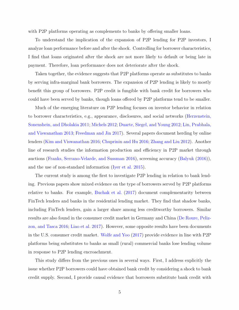
To visualize the timing of the effect of the bank credit shock, I start by replacing the

Post dummy in Equation (1) with year-quarter dummies and then plot the coefficients on the

year-quarter dummies interacted with the Treated dummy in Figure 4. P2P lending volume

in the quarter preceding the policy change (2010Q4) is used as the reference level. Green

dots represent loan applications and orange triangles represent funded loans. It shows that

P2P application and origination volumes increase significantly in affected counties relative

to control counties after the negative shock to bank credit supply, both in terms of the total

loan amount (Panel a) and the number of loans (Panel b). In addition, there is no significant

difference in P2P lending volume between treated counties and control counties before the

shock. The absence of pre-shock trend reasures that the increase in demand for P2P credit

is unlikely to be driven by unobservable differences between treated and control markets.

When I turn to predictions regarding the composition of borrowers in Sections 6.2 and

6.3, it will be preferable to work with annual data in order to obtain more precise measures

of the statistical features (e.g., quantiles) of the borrower quality distribution at the county-

10The data on economic indices and demographics are from the Bureau of Economics Analysis.

17

time level. Thus, I re-estimate Equation (1) for P2P lending volume at the county-year

level and tabulate the results in Table 3. Consistent with Figure 4, I find that, relative to

control counties, affected counties experience an average increase in P2P loan application

of USD 1,108 (column 1) or 0.070 additional loan applications (column 2) per thousand

inhabitants. It represents 25.3% and 38.7% of the corresponding pre-shock levels (2,648

USD or 0.256 applications per thousand inhabitants). This higher demand is satisfied by

the P2P platform. The lending volume increases by USD 301 (column 3) or 0.016 additional

originations (column 4), representing 1.5 times the pre-shock level of the dollar amount

originated and 1.1 times the pre-shock level of the number of originations.

To summarize, the results on P2P volume show that when banks cut lending in the

consumer credit market, borrowers switch from traditional financial institutions to P2P

platforms. This finding is consistent with P2P platforms and banks being either complements

or substitutes (Predictions on Volume). I now turn to testing the Predictions on Distribution

and Frequency of P2P borrowers where substitutability and complementarity lead to opposite

predictions.

6.2 Predictions on Distribution

The Predictions on Distribution imply that if banks and P2P platforms are substitutes, the

reduction in bank credit leads to a drop in the average quality of P2P borrowers and a

decrease in the quantiles of the borrower quality distribution, whereas these predictions are

reversed if banks and P2P platforms are complements.

To test these predictions, I estimate Equation (1) using the mean and quantiles of the

borrower quality distribution as dependent variables. Table 4 reports the results when bor-

rower quality is measured by the FICO score (Panel A) and by the predicted borrower

quality (Panel B). A first look at the results reveals that, for both proxies of borrower qual-

ity, the quantiles (columns 1 to 10) as well as the mean (column 11) decrease simultaneously

in treated counties relative to control counties, which is consistent with banks and P2P

platforms being substitutes.

A closer look at the results allows me to make the interpretation more precise. First,

the drop in the average borrower quality is not statistically significant at the conventional

18

level (p-value equal to 0.12 in Panel A and 0.17 in Panel B). The reason can be grasped

by inspecting more closely the effect on the quantiles. Using the FICO score to measure

borrower quality, I find that while all quantiles decrease, the effect is statistically significant

only above the 45th percentile. It suggests that the FICO scores of new borrowers are

below the 45th percentile (equal to 690) of the pre-shock distribution of P2P borrowers’

FICO scores. The frequency analysis in Section 6.3 will allow me to confirm and refine this

conclusion.

Second, when using predicted borrower quality as a measure of quality, all the quantiles

still decrease but the effect is now significant only at the 5th percentile. The interpretation

is that while the borrowers rejected by banks who manage to obtain funding from the P2P

platform belong to the bottom half of the FICO distribution, they belong to the very left tail

of the quality distribution when the debt-to-income ratio and employment length are also

taken into account. A possible explanation for this result is that the P2P platform imposes

strict requirement on the FICO score but not on other borrower characteristics. It implies

that the worsening of borrower quality is more visible on other dimensions than the FICO

score.

The results on the change in the distribution of P2P borrower quality are thus consistent

with banks and P2P platforms being substitutes. The analysis of quantiles has, however, one

limitation when it comes to detect the range of the distribution in which new P2P borrowers

rejected by banks are located. To see it, suppose for instance that all new P2P borrowers are

between the 5th and the 45th percentiles. The regressions of quantiles will then show that

all the quantiles from the 5th to the 95th decrease, failing to identify that the additional

mass of borrowers stops at the 45th percentile. To overcome this limitation of the quantile

analysis, I now analyze the frequency distribution of borrower quality.

6.3 Predictions on Frequency

The Predictions on Frequency are that, if banks and P2P platforms are substitutes, the

increased demand for P2P credit will come from low-quality borrowers, leading to a higher

number of borrowers only in the low-quality spectrum of the distribution. Instead, if P2P

platforms operate as complements to banks, the increase in the number of borrowers will

19

occur in the high-quality part of the distribution.

To test this prediction, I estimate Equation (1) using the number of P2P borrowers in

each of the twenty-point-wide FICO score intervals between 650 and 850 as the dependent

variable. The estimated coefficients are plotted in the top panel of Figure 5(a). I find that

the increase in P2P lending volume is driven by the bottom two FICO score intervals, ranging

from 650 to 690.

To interpret more precisely this result, I compare the estimated change in the frequency

distribution (top panel) to the pre-shock distribution of P2P borrowers’ FICO scores (bottom

panel). The prediction is that, if banks and P2P borrowers are substitutes, the increase in

the frequency distribution should be located in the left part of the support of the pre-shock

distribution (see Figure 1), whereas if they are complements, the increase should be located

to the right of the support of the pre-shock distribution (see Figure 2).

This is exactly what I find. More specifically, in the interval of FICO score between 650

and 690, which corresponds to FICO scores below the 45th percentile of the pre-shock distri-

bution, the number of originations increases by 0.013 per thousand inhabitants (significant

at 1% level), or 1.9 times of the pre-shock level. In contrast, the the number of originations

does not increase significantly in other intervals where the FICO score is above 690. Thus,

the increase in P2P lending induced by the shock to bank credit supply is located at the

lower end of the P2P borrower quality distribution, consistent with P2P platforms and banks

being substitutes.

I obtain similar results using predicted quality as the measure of borrower quality as

reported in Figure 5(b). The top panel shows that the increase is located between 0.1 and

0.4, corresponding to the levels of predicted borrower quality below the 20th percentile of

the pre-shock distribution. Comparing the top panel to the pre-shock distribution of pre-

dicted borrower quality in the bottom panel, we observe that the increase in the frequency

distribution is indeed located in the left part of the pre-shock distribution. More specifi-

cally, the total number of originations in the bottom four intervals increases by 0.009 per

thousand inhabitants (significant at 5% level), amounting to 1.3 times the pre-shock level.

In contrast, the change in the other six intervals are not significant. These results suggest

a disproportionally high growth in loan originations in low-quality intervals compared to in

20

high-quality intervals.

Overall, the results in this section indicate that following the tightening of banks’ lending

criteria, P2P platforms experience an increase in originations among low-quality borrowers,

in line with P2P platforms being substitutes to banks.

7 Additional Results

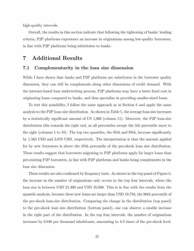
7.1 Complementarity in the loan size dimension

While I have shown that banks and P2P platforms are substitutes in the borrower quality

dimension, they can still be complements along other dimensions of credit demand. With

the internet-based loan underwriting process, P2P platforms may have a lower fixed cost in

originating loans compared to banks, and thus specialize in providing smaller-sized loans.

To test this possibility, I follow the same approach as in Section 6 and apply the same

analysis to the P2P loan-size distribution. As shown in Table 5, the average loan size increases

by a statistically significant amount of US 1,066 (column 11). Moreover, the P2P loan-size

distribution tilts towards the right end, as all percentiles except the 5th percentile move to

the right (columns 1 to 10). The top two quantiles, the 85th and 95th, increase significantly

by 1,563 USD and 3,870 USD, respectively. The interpretation is that the amount applied

for by new borrowers is above the 85th percentile of the pre-shock loan size distribution.

These results suggest that borrowers migrating to P2P platforms apply for larger loans than

pre-existing P2P borrowers, in line with P2P platforms and banks being complements in the

loan size dimension.

These results are also confirmed by frequency tests. As shown in the top panel of Figure 6,

the increase in the number of originations only occurs in the top four intervals, where the

loan size is between USD 21,400 and USD 35,000. This is in line with the results from the

quantile analysis, because these new loans are larger than USD 19,750, the 90th percentile of

the pre-shock loan-size distribution. Comparing the change in the distribution (top panel)

to the pre-shock loan size distribution (bottom panel), one can observe a sizable increase

in the right part of the distribution. In the top four intervals, the number of originations

increases by 0.048 per thousand inhabitants, amounting to 4.3 times of the pre-shock level.

21

In contrast, none of the changes in other intervals is statistically significant at 5% level.

Taken together, the results on loan size suggest that P2P platforms complement banks by

serving small-sized loans. This conclusion is subject to a caveat, however. The predictions

generated by the simple framework in Section 2 rely on the assumption that banks curtail

lending in the left part of the bank borrower distribution. This assumption is satisfied in the

borrower quality dimension in my empirical setup, as FAS 166/167 leads banks to tighten

credit standards, but it may not hold on the loan size dimension.

7.2 Plausibility of the assumption of elastic P2P credit supply

One of the assumptions in the framework presented in Section 2 is that the supply of P2P

credit is elastic. It implies that an increase in the demand for P2P credit will not lead to a

change in the interest rate. I now provide some empirical evidence to show the plausibility

of this assumption.

If P2P credit supply is elastic, one should observe the following. First, at the platform

level, P2P platforms do not adjust interest rates or screen borrowers based on local demand

for P2P credit. Second, at the investor level, in response to the increased demand, P2P

investors increase credit supply. In other words, the probability of loan listings being funded,

after passing the initial screening by the platform, does not decrease.

I examine these two predictions one by one. I first show that interest rates set by the

platform depend neither on the location of borrowers nor on the level of local demand for

P2P credit following the negative shock to bank credit supply. Second, I present evidence

that the probability of a loan listing being funded does not vary before and after the shock,

conditional on loan characteristics.

7.2.1 LendingClub pricing policy

As explained in Section 3, according to LendingClub’s prospectus, the interest rates on P2P

loans do not depend on the location of borrowers. To verify whether this is actually the case,

I test the joint significance of county fixed effects in the following regression:

yi,c,t “ γc ` βTreatedc ˆ Postt ` σt ` LoanControlsi,c,t ` εi,c,t,

22

where loans are indexed by i, counties by c, and quarters by t; yi,c,t is the loan grade or the

interest rate of loan i; γc is the fixed effect for county c; TreatedˆPost is the interaction term

used in the main specification; σt is quarter t’s fixed effect; and LoanControlsi,c,t includes

loan and borrower characteristics.

I implement two sets of tests using the loan grade and the interest rate as dependent

variables, because the platform sets the interest rate in two steps (see Section 3): it first

assigns a loan grade based on borrower and loan characteristics, and then sets an interest

rate based on loan grade and other factors. Hence, I first estimate the above equation using

LendingClub’s loan grade as the dependent variable. The loan grade takes 35 possible values,

from A1 to G5. I assign 1 to 35 to each loan grade with lower numbers representing better

grades. Second, I use the interest rate as the dependent variable, controlling for the loan

grade.

If geography does not affect LendingClub’s loan grade and interest rate, the county fixed

effects should be zero in either regression. Similarly, if interest rates do not respond to local

demand for P2P credit, the coefficient of the interaction term Treated ˆ Post should also

be zero.

Table 6 reports the regression results as well as F -statistics and p-values of the test

on the joint significance of county fixed effects γc. As predicted, the county fixed effects

are insignificant in all columns. The p-values of the test of the joint significance of county

fixed effects are 0.188 (column 1) and 0.958 (column 3) when the dependent variable is

loan grade and interest rate, respectively. Therefore, I fail to reject the null hypothesis

that LendingClub’s pricing policy is independent of borrower location. Moreover, as shown

in columns 2 and 4, the estimated coefficients of Treated ˆ Post is insignificant with t-

statistics of -0.01 and -0.067. This implies that despite an increased demand for P2P credit

in affected markets, interest rates do not adjust upwards for loans from those markets.

7.2.2 Investor funding behavior

Do P2P investors respond to an increased demand by raising credit supply, even though the

interest rate does not increase? I show below that conditional on passing the initial screening

by the platform, a loan listing has the same probability of being funded before and after the

23

shock.

Using the data on loan listings, i.e., loan applications that have passed the initial screening

procedure,11 I estimate the following probit model:

EpFundedi,c,t|Treated, Post, Controlsq

“PrpFundedi,c,t “ 1|Treated, Post, Controlsq

“βTreatedc ˆ Postt ` γc ` σt ` Controlsi,c,t,

where Fundedi,c,t is an indicator that takes value one if the listing received full funding and

zero otherwise. If credit supply does not increase as much as the demand for credit, or if

credit supply is even reduced, one will observe a negative β, i.e., a smaller fraction of loans

will be funded after the shock.

Table 7 reports the results. In the first column, I do not include Controlsi,c,t. The

county-level and loan-level control variables are gradually added to the regressions in the

subsequent columns, while year and county fixed effects are always included. Across all

specifications, the coefficient on Treated ˆ Post is never significant. This result suggests

that investors increase credit supply as a response to the increase in the demand for P2P

credit even though the interest rate remains constant.

Overall, the evidence presented in this section is consistent with a perfectly elastic supply

of P2P credit at the local market level, as assumed in the conceptual framework.

7.3 Implications for P2P Investors

The above results suggest that infra-marginal borrowers benefit from the expansion of P2P

platforms, but remain silent about the effects on investors. I now examine the implications

of the expansion of P2P lending on P2P investors. Specifically, I investigate whether the loan

performance deteriorates when low-quality borrowers substitute bank credit with P2P credit.

This would be true if the higher credit risk brought about by the worsening of the pool of

P2P borrowers, following the negative shock to bank credit supply, is not or is imperfectly

reflected in the interest rate.

11The data on loan listings are not available on LendingClub’s website. I obtain this data from Lending-Club’s filings with SEC.

24

Since almost all loans originated no later than 2012 have reached maturity at the time

of the data collection, I observe loan status. A loan can be fully paid, in grace period (late

for 1-15 days), late for 16-120 days, charged off, or in default. I categorize a loan as non-

performing if the loan is not paid in full, and test whether loan performance worsens in

affected counties after the shock, controlling for interest rate. Now working at the loan level,

I regress the non-performing loan dummy on the interest rate, the treated county dummy

interacted with the post-FAS 166/167 dummy, as well as county and year fixed effects.

The results are reported in Table 8. In column 1, I check whether the interest rate predicts

loan non-performance. Indeed, it does so with a high level of statistical significance (a t-

statistic of 50). In column 2, I add the Treatedˆ Post and find an insignificant coefficient.

Adding the loan-level control variables (column 3) and the county-level control variables

(column 4) yields similar results. To summarize, the worsening of the borrower pool is priced

into interest rate, and therefore loan performance does not deteriorate after controlling for

interest rate.

8 Concluding Remarks

The fast emergence of P2P lending after the 2008 financial crisis opens a hotly debated

question about its consequences. The answer to the question crucially depends on whether

the P2P industry merely displaces the incumbents or fills the gap in an under-served credit

market. This paper provides insights on this debate by examining the relation between P2P

platforms and banks. Exploiting a negative shock to bank credit supply, I show that P2P

lending expands in the markets exposed to this shock. I also find evidence for substitution

between banks and P2P platforms based on the fact that, when low-quality bank borrowers

migrate to P2P platforms, P2P borrower pool worsens. This result suggests that the credit

expansion opportunities brought by P2P lenders are likely to occur only for infra-marginal

bank borrowers. On the other hand, P2P platforms complement banks by focusing on the

market segment for small loans. The amount requested by borrowers migrating from banks

to P2P platforms is larger than 90% of pre-existing P2P loans.

Although the empirical analysis carried out in the paper uses data from the largest P2P

lending platform in the U.S., two caveats are in order. First, the empirical analysis focuses

25

on the unsecured consumer loan market. The results may not generalize to other markets

such as the residential lending market, or to other countries with a different banking market

structure than the U.S. Second, the landscape of the FinTech industry is changing rapidly.

Therefore, P2P platforms may not operate as substitutes to banks in the long run. That being

said, it is noteworthy that notwithstanding the rapid growth of the sector, LendingClub was

the dominant player in the P2P unsecured consumer loan market during my sample period

2019-12, and is still so in 2018, .

26

References

Balyuk, T. 2016. Financial innovation and borrowers: Evidence from peer-to-peer lending .

Buchak, G., G. Matvos, T. Piskorski, and A. Seru. 2017. Fintech, regulatory arbitrage, and

the rise of shadow banks. Working Paper, National Bureau of Economic Research.

Chuprinin, O., and M. R. Hu. 2016. Herding and capital allocation efficiency: Evidence from

peer lending .

De Roure, C., L. Pelizzon, and P. Tasca. 2016. How does p2p lending fit into the consumer

credit market? .

Dou, Y. 2016. Spillover effects of consolidating securitization entities on small business

lending. Available at SSRN 2727958 .

Dou, Y., S. G. Ryan, and B. Xie. 2016. The real effects of fas 166 and fas 167 .

Duarte, J., S. Siegel, and L. Young. 2012. Trust and credit: the role of appearance in

peer-to-peer lending. Review of Financial Studies 25:2455–84.

Franks, J., N. Serrano-Velarde, and O. Sussman. 2016. Marketplace lending, information

effciency, and liquidity .

Freedman, S., and G. Z. Jin. 2017. The information value of online social networks: lessons

from peer-to-peer lending. International Journal of Industrial Organization 51:185–222.

Herzenstein, M., S. Sonenshein, and U. M. Dholakia. 2011. Tell me a good story and I

may lend you money: The role of narratives in peer-to-peer lending decisions. Journal of

Marketing Research 48:S138–49.

Iyer, R., A. I. Khwaja, E. F. Luttmer, and K. Shue. 2015. Screening peers softly: Inferring

the quality of small borrowers. Management Science 62:1554–77.

Kim, K., and S. Viswanathan. 2016. The “experts” in the crowd: The role of’expert’investors

in a crowdfunding market .

27

Liao, L., Z. Wang, H. Xiang, and X. Zhang. 2017. P2p lending in china: An overview .

Lin, M., N. R. Prabhala, and S. Viswanathan. 2013. Judging borrowers by the company

they keep: Friendship networks and information asymmetry in online peer-to-peer lending.

Management Science 59:17–35.

Michels, J. 2012. Do unverifiable disclosures matter? evidence from peer-to-peer lending.

The Accounting Review 87:1385–413.

Tian, X. S., and H. Zhang. 2016. Impact of FAS 166/167 on credit card securitization .

White, L. J. 1987. Antitrust and merger policy: a review and critique. The Journal of

Economic Perspectives 1:13–22.

Wolfe, B., and W. Yoo. 2017. Crowding out banks: Credit substitution by peer-to-peer

lending .

Zhang, J., and P. Liu. 2012. Rational herding in microloan markets. Management science

58:892–912.

28

Figures and Tables

Figure 4: P2P Lending Volume around FAS 166/167

(a) Dollar amount (b) Number of loans

-150

015

030

0

-500

050

010

00

-8 -7 -6 -5 -4 -3 -2 1 2 3 4 5 6 7 8Quarters since FAS 166/167

$ application (left axis) $ funded (right axis)

-.005

50

.005

5.0

11.0

165

-.02

0.0

2.0

4.0

6

-8 -7 -6 -5 -4 -3 -2 1 2 3 4 5 6 7 8Quarters since FAS 166/167

# application (left axis) # funded (right axis)

Notes: This figure reports the effects of FAS 166/167 on local P2P application volume (green dots) and origination volume

(orange triangle), obtained from the estimates of Equation (1) at with the quarterly data. The left (right) vertical axis represents

the magnitude of the green dots (orange triangle). P2P lending volume is measured in dollar amount per thousand inhabitants

in panel (a) and by the number of loans per thousand inhabitants in panel (b). Quarter t “ ´1 denotes the last quarter of 2010

and is used as the reference point. Error bars show 95% confidence intervals. Standard errors are clustered at county level.

29

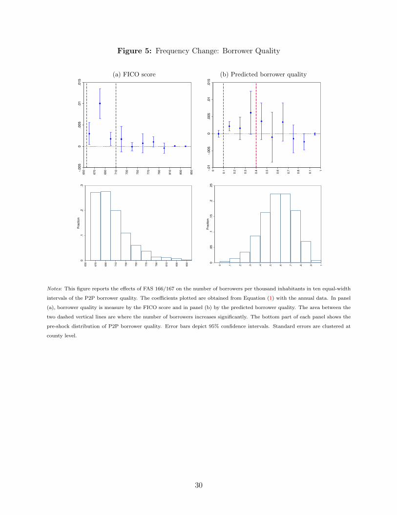
Figure 5: Frequency Change: Borrower Quality

(a) FICO score (b) Predicted borrower quality-.005

0.005

.01

.015

650

670

690

710

730

750

770

790

810

830

850

0-.0

1-.0

05.0

05.0

1.0

150

0.1

0.2

0.3 0.4

0.5

0.6

0.7

0.8

0.1 1

0.1

.2.3

Fraction

650

670

690

710

730

750

770

790

810

830

850 0

.05

.1.15

.2.25

Fraction

0 .1 .2 .3 .4 .5 .6 .7 .8 .9 1

Notes: This figure reports the effects of FAS 166/167 on the number of borrowers per thousand inhabitants in ten equal-width

intervals of the P2P borrower quality. The coefficients plotted are obtained from Equation (1) with the annual data. In panel

(a), borrower quality is measure by the FICO score and in panel (b) by the predicted borrower quality. The area between the

two dashed vertical lines are where the number of borrowers increases significantly. The bottom part of each panel shows the

pre-shock distribution of P2P borrower quality. Error bars depict 95% confidence intervals. Standard errors are clustered at

county level.

30

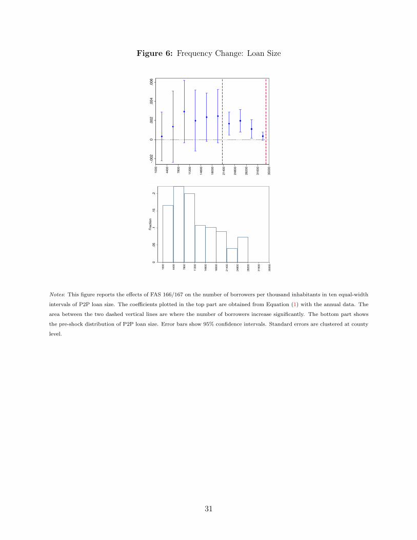
Figure 6: Frequency Change: Loan Size

-.002

0.002

.004

.006

1000

4400

7800

11200

14600

18000

21400

24800

28200

31600

35000

0.05

.1.15

.2Fraction

1000

4400

7800

11200

14600

18000

21400

24800

28200

31600

35000

Notes: This figure reports the effects of FAS 166/167 on the number of borrowers per thousand inhabitants in ten equal-width

intervals of P2P loan size. The coefficients plotted in the top part are obtained from Equation (1) with the annual data. The

area between the two dashed vertical lines are where the number of borrowers increase significantly. The bottom part shows

the pre-shock distribution of P2P loan size. Error bars show 95% confidence intervals. Standard errors are clustered at county

level.

31

Table 1: Summary Statistics: LendingClub Loans

Min Mean Max Std. Dev. Num. of observations

Panel A. All applications

Amount 1,000 1,3104 35,000 10,111 880,346FICO score 457 666 815 82.988 880,346DTI 0.000 0.188 1.000 0.162 880,346LengthEmploy 0 2.053 11 3.553 880,346

Panel B. Funded loans

Interest rate 0.054 0.133 0.249 0.043 93,159Amount 1,000 13,224 35,000 8,426 93,159Maturity 0 0.135 1 0.342 93,159DTI 0 0.147 0.332 0.079 93,159FICO score 660 711 848 38 93,159Predicted borrower quality 0 0.568 1 0.163 93,159Mortgage 0 0.439 1 0.496 93,159Home owner 0 0.106 1 0.308 93,159Delinquency 0 0 1 0.016 93,159Revolving balance 0 14,054 86,557 14,504 93,159Total credit line 4 22.383 56 11.235 93,159Open accounts 2 9.823 23 4.497 93,159Revolver utilization 0 52.125 97.400 27.286 93,159Inquiries last6m 0 0.953 5 1.151 93,159Delinquency last2yers 0 0.174 3 0.506 93,159LengthEmploy 0 5.703 11 3.929 93,159LengthCredit 4 14.358 38 7.081 93,159

Notes: This table presents summary statistics of LendingClub loan characteristics for all loan applications (Panel A) and fundedloans (Panel B). The definition of each variable is provided in Table A1 in Appendix A.

32

Table 2: Summary Statistics: County Characteristics

Min Mean Max Std. Dev. Num. of observations

Panel A. Lending Volume

$ applications (in thousands) 0 776.090 240,235 4,012 15,180

# applications 0 76 16,278 288 15,180

$ funded loans (in thousands) 0 77.911 33,177 506.440 15,180

# funded loans 0 6 2,526 37 15,180

Panel B. Normalized lending volume

$ applications/(population/1000) 0 7,665 291,908 10,329 11,794

# applications/(population/1000) 0 0.585 18.935 0.701 11,794

$ funded loans/(population/1000) 0 604 50,457 1,387 11,794

# funded loans/(population/1000) 0 0.048 2.014 0.096 11,794

Panel C. Other variables

Treated 0 0.662 1 0.473 12,134

HHI 466 3,118 10,000 2041.191 12,058

Share(small banks) 0 0.389 1 0.402 12,058

Share(national banks) 0 0.154 1 0.271 12,058

Geo. diversification 1 3.037 40 4.642 12,058

Deposit 1,434 17809 1,795,294 24,379 11,728

Population 258 103,742 10,045,175 324,247 11,794

Personal income 14,360 35,298 176,046 9,681 11,794

Unemployment rate 1.600 8.922 28.900 3.026 11,795

Notes: This table shows the summary statistics of the county-level variables. Panels A and B report the overall P2P lendingvolume and the normalized P2P lending volume, respectively. Panel C presents other county-level variables. Treated is abinary dummy variable that takes value 1 if there is at least one bank affected by FAS 166/167 in the county. HHI measuresmarket competition in the local banking industry. Sharepsmall banksq is the share of banks with total assets below one billion;Sharepnational banksq is the share of national banks. Geo. diversification is a proxy for the geographical diversification ofbanks, measured by the median number of the states in which the banks in a given county operate. Deposit is the depositper thousand inhabitants in a county. Personal income is the median annual personal income, in USD. Unemployment is theunemployment rate (in percentage points) in a given year in a county.

33

Table 3: The Impact of FAS 166/167 on LendingClub Demand and Supply

Applications Funded loansAmount($) Number(#) Amount($) Number(#)

(1) (2) (3) (4)

Treated ˆ Post 1107.690*** 0.070*** 300.542*** 0.016***(2.888) (2.918) (6.310) (4.741)

1000 ď HHI ă 1800 65.618 -0.019 -17.221 -0.000

(0.130) (-0.561) (-0.191) (-0.019)

HHI ě 1800 151.585 -0.014 -36.821 0.000

(0.242) (-0.343) (-0.348) (0.024)

Share(small banks) 182.530 0.026 162.522 0.013(0.163) (0.366) (1.452) (1.614)

Share(national banks) -1159.254 -0.014 383.648 0.029*(-1.291) (-0.236) (1.473) (1.794)

Geo. diversification 140.281** 0.013*** 36.014 0.002*(2.167) (3.055) (1.481) (1.696)

Population -0.049*** -0.000*** -0.011*** -0.000***(-5.157) (-5.225) (-5.613) (-5.651)

Deposit 0.004*** 0.000*** 0.001*** 0.000***(3.098) (2.953) (2.617) (4.038)

Personal income 0.013 0.000** 0.005 0.000(0.354) (2.235) (0.819) (1.316)

Unemployment rate 747.445*** 0.046*** 79.788*** 0.005***(6.339) (6.521) (3.792) (4.885)

Year FE Y Y Y YCounty FE Y Y Y Y

Observations 11,726 11,726 11,726 11,726R2 0.710 0.756 0.532 0.557

Notes: This table reports the impact of the bank credit supply shock on P2P application and origination volumes, which isestimated from the following regression with the county-year data during 2009-12:

yc,t “ βTreatedc ˆ Postt ` Controlsc,t ` γc ` σt ` εc,t.

The dependent variable is P2P application volume or P2P origination volume. Application volume is measured by either thetotal amount demanded in loan applications per thousand inhabitants (column 1) or the total number of loan applications perthousand inhabitants (column 2) in a given county. The same method is applied to the origination volume in columns 3 and 4.Treated is an indicator for whether there are affected banks in the county. Post takes value 1 from 2011 on and 1 before. Othercounty-level control variables are defined in Table A1. Year and county fixed effects are included in all regressions. t-statisticsare in parentheses. Standard errors are clustered at county level. * p ă 0.10, ** p ă 0.05, *** p ă 0.01.

34

Table 4: Changes in Post-shock Distributions of P2P Loans: Borrower Quality

PercentileMean

5th 15th 25th 35th 45th 55th 65th 75th 85th 95th(1) (2) (3) (4) (5) (6) (7) (8) (9) (10) (11)

Panel A. FICO score

TreatedˆPost -2.357 -0.317 -0.046 -2.402 -2.148 -8.675*** -7.996** -8.790** -6.716* -1.175 -3.707(-0.744) (-0.100) (-0.015) (-0.752) (-0.680) (-2.610) (-2.311) (-2.384) (-1.710) (-0.286) (-1.562)

Panel B. Predicted borrower quality

TreatedˆPost -0.053*** -0.021 -0.006 -0.013 -0.008 -0.023 -0.017 -0.024 -0.020 -0.007 -0.020(-3.060) (-1.222) (-0.396) (-0.843) (-0.532) (-1.543) (-1.124) (-1.590) (-1.352) (-0.464) (-1.396)

Controls Y Y Y Y Y Y Y Y Y Y YYear FE Y Y Y Y Y Y Y Y Y Y YCounty FE Y Y Y Y Y Y Y Y Y Y YN 5,059 5,059 5,059 5,059 5,059 5,059 5,059 5,059 5,059 5,059 5,059

Notes: This table reports the impact of the bank credit supply shock on the quantiles and the mean of the borrower qualitydistribution, which is estimated from the following regression with the county-year data during 2009-12:

yc,t “ βTreatedc ˆ Postt ` Controlsc,t ` γc ` σt ` εc,t.

In each of columns 1-10, the dependent variable the kth (k P t5, 15, . . . , 95u) percentile of the distribution of FICO scores (PanelA) and predicted borrower quality (Panel B). In column 11, the dependent variable is the average borrower quality. All columnsinclude the same set of baseline controls as in Table 3 as well as county and year fixed effects. t-statistics are in parentheses.Standard errors are clustered at county level. * p ă 0.10, ** p ă 0.05, *** p ă 0.01.

35

Table 5: Changes in Post-shock Distributions of P2P Loans: Loan Size

PercentileMean

5th 15th 25th 35th 45th 55th 65th 75th 85th 95th(1) (2) (3) (4) (5) (6) (7) (8) (9) (10) (11)

TreatedˆPost -431.227 133.105 539.770 315.903 782.406 122.866 860.915 955.827 1562.936** 3869.708*** 1066.046**(-0.774) (0.240) (1.003) (0.559) (1.360) (0.209) (1.456) (1.433) (2.049) (4.819) (2.043)

Controls Y Y Y Y Y Y Y Y Y Y YYear FE Y Y Y Y Y Y Y Y Y Y YCounty FE Y Y Y Y Y Y Y Y Y Y Y

N 5,059 5,059 5,059 5,059 5,059 5,059 5,059 5,059 5,059 5,059 5,059

Notes: This table reports the impact of the bank credit supply shock on the quantiles and the mean of the loan size distribution,which is estimated from the following regression with the county-year data during 2009-12:

yc,t “ βTreatedc ˆ Postt ` Controlsc,t ` γc ` σt ` εc,t.

In each of columns 1-10, the dependent variable the kth (k P t5, 15, . . . , 95u) percentile of the loan size distribution. In column11, the dependent variable is the average loan size. All columns include the same set of baseline controls as in Table 3 as wellas county and year fixed effects. t-statistics are in parentheses. Standard errors are clustered at county level. * p ă 0.10, **p ă 0.05, *** p ă 0.01.36

Table 6: Testing the Elastic Supply of P2P Credit

Loan grade Interest rate(1) (2) (3) (4)

Panel A: Test results

Number of counties 1,925 1,925 1,925 1,925

F(1925, 89,839) 1.029 1.029 0.945 0.944

p-value 0.188 0.186 0.958 0.958

Panel B: Estimated coefficients

Treated ˆ Post -0.00186 -0.254(-0.010) (-0.067)

Amount 0.000244*** 0.000244*** 0.000317*** 0.000317***(157.750) (157.745) (9.133) (9.136)

Loan term 6.185*** 6.185*** 10.38*** 10.39***(225.074) (225.080) (15.139) (15.152)

FICO score2 0.000933*** 0.000933*** 0.00206*** 0.00206***(147.587) (147.582) (14.582) (14.583)

FICO score -1.472*** -1.472*** -2.616*** -2.616***(-156.443) (-156.439) (-12.301) (-12.304)

DTI -13.42*** -13.44*** 1804.2*** 1803.8***(-4.360) (-4.367) (30.179) (30.173)

FICO score ˆ DTI 0.000583 0.000615 -2.507*** -2.506***(0.143) (0.151) (-31.670) (-31.664)

DTI2 33.11*** 33.11*** -29.49 -29.60(20.739) (20.733) (-0.949) (-0.952)

LengthEmploy -0.0394*** -0.0393*** 0.105 0.107(-3.696) (-3.685) (0.510) (0.518)

LengthEmploy2 0.00337*** 0.00336*** -0.000775 -0.000965(3.910) (3.895) (-0.046) (-0.058)

LengthCredit -0.143*** -0.143*** 0.874*** 0.874***(-22.030) (-22.026) (6.934) (6.936)

LengthCredit2 0.00324*** 0.00323*** -0.0223*** -0.0223***(18.995) (18.993) (-6.741) (-6.741)

Mortgage -0.354*** -0.355*** -3.703*** -3.707***(-14.391) (-14.400) (-7.735) (-7.743)

Own 0.0133 0.0133 -1.109 -1.110(0.327) (0.325) (-1.399) (-1.400)

Current delinquency -1.804** -1.805** 28.60* 28.59*(-2.161) (-2.163) (1.766) (1.765)

Revolving balance -0.0000135*** -0.0000135*** -0.000106*** -0.000106***(-14.588) (-14.582) (-5.899) (-5.896)

Total credit lines -0.00332** -0.00329** 0.0980*** 0.0984***(-2.356) (-2.335) (3.579) (3.595)

Open accounts -0.00694** -0.00696** 0.285*** 0.284***(-2.031) (-2.038) (4.292) (4.287)

Revolver utilization 0.0299*** 0.0299*** 0.0184* 0.0184*(55.464) (55.464) (1.719) (1.722)

Inquiries last6m 0.751*** 0.751*** 1.809*** 1.810***(74.147) (74.147) (8.700) (8.703)

Delinquency last2yrs 0.253*** 0.253*** 0.288 0.287(11.888) (11.884) (0.696) (0.694)

Year-quarter FE Y Y Y YLoan grade FE N N Y YObservations 89,839 89,837 89,839 89,837R2 0.801 0.801 0.982 0.982

Notes: This table reports the test results of the elastic supply of P2P credit using the following regression equation, estimatedat loan level during 2009-12:

yi,c,t “ γc ` βTreatedc ˆ Postt ` LoanControlsi,c,t ` σt ` εi,c,t.

The dependent variable is either the loan grade assigned by LendingClub (columns 1-2) or the interest rate (in basis point)(columns 3-4). In all columns, loan and borrower characteristics are included. In columns 2 and 4, the interaction termTreatedˆ Post is included. The F -statistic and p-value of the test on the joint significance of county fixed effects are reportedin Panel A. Standard errors are clustered at county level. t statistics are in parentheses. * p ă 0.10, ** p ă 0.05, *** p ă 0.01.

37

Table 7: Probability of Loan Listings Being Funded

Dependent variable = 1 if funded(1) (2) (3) (4)

Treated ˆ Post -0.016 -0.031 -0.098 -0.113(-0.252) (-0.430) (-1.303) (-1.371)

Interest Rate -13.427*** -13.337***(-45.898) (-42.736)

Amount 4.6e-6** 4.8e-6**(2.259) (2.154)

Amount ˆ Interest rate -0.000*** -0.000***(-10.498) (-9.800)

FICO score -0.086*** -0.086***(-22.276) (-21.086)

FICO score2 0.000*** 0.000***(21.200) (20.057)

DTI 16.972*** 16.702***(12.996) (12.002)

DTI2 -18.921*** -18.711***(-31.131) (-29.423)

FICO score ˆ DTI -0.015*** -0.015***(-8.683) (-7.936)

LengthEmploy 0.014 0.014(0.802) (0.657)

LengthEmploy2 -0.001* -0.001(-1.872) (-1.489)

LengthCredit 0.014*** 0.013***(4.886) (4.255)

LengthCredit2 -5.0e-4*** -4.8e-4***(-7.082) (-6.318)

Mortgage 0.012 0.011(1.230) (1.031)

Home owner -0.295*** -0.302***(-20.097) (-19.582)

Delinquency -0.851*** -0.907***(-2.946) (-2.983)

Revolving balance -5.4e-6*** -5.5e-6***(-15.675) (-15.649)

Total credit line 0.005*** 0.006***(8.107) (8.321)

Open accounts 0.009*** 0.009***(6.323) (5.628)

Revolver utilization 0.007*** 0.007***(28.654) (26.782)

Inquiries last6m -0.079*** -0.077***(-17.014) (-14.869)

Delinquency last2yrs -0.010 -0.013(-1.186) (-1.496)

County Controls N Y N YYear FE Y Y Y YCounty FE Y Y Y Y

# Observations 154,046 135,867 123,714 109,363Pseudo R2 0.018 0.018 0.152 0.151

Notes: This table reports the impact of the shock to the bank credit supply on the probability of P2P loans listings beingfunded. The estimates are from the following probit model with the loan level data during 2009-12:

EpFundedi,c,t|Treated, Post, Controlsq

“PrpFundedi,c,t “ 1|Treated, Post, Controlsq

“βTreatedc ˆ Postt ` γc ` σt ` Controlsi,c,t,

where the dependent variable is an indicator that takes value 1 if the loan listing is funded and 0 otherwise. In column 1,the interaction term is included as the explanatory variable. In columns 2 and 4, county level control variables are included.In columns 3 and 4, borrower characteristics and loan characteristics are included. Year and county fixed effects are alwaysincluded. t-statistics are in parentheses. Standard errors are clustered at county level. * p ă 0.10, ** p ă 0.05, *** p ă 0.01.

38

Table 8: Loan Performance

Dependent variable = 1 if non-performing(1) (2) (3) (4)

Interest Rate 7.470*** 7.470*** 5.140*** 5.120***(50.510) (50.501) (13.691) (13.553)

Treated ˆ Post 0.076 0.062 0.046(0.588) (0.500) (0.351)

Amount ˆ Interest Rate -0.000 -0.000(-0.885) (-0.920)

Amount 0.000 0.000(0.749) (0.745)

Maturity 0.293*** 0.293***(16.781) (16.771)

FICO score 0.020*** 0.021***(3.326) (3.423)

FICO score2 -0.000*** -0.000***(-3.565) (-3.655)

DTI 3.994** 4.410**(2.265) (2.493)

DTI2 0.857 0.809(0.934) (0.875)

FICO score ˆ DTI -0.005** -0.005**(-2.041) -0.005**

LengthEmploy -0.006 -0.007(-0.979) (-1.066)

LengthEmploy2 0.001 0.001(1.457) (1.528)

LengthCredit -0.001 -0.001(-0.330) (-0.296)

LengthCredit2 0.000 0.000(0.612) (0.612)

Mortgage -0.086*** -0.087***(-6.164) (-6.131)

Home owner -0.013 -0.011(-0.598) (-0.505)

Revolving balance -0.000*** -0.000***(-7.231) (-7.084)

Total credit lines -0.005***(-6.618) (-6.582)

Open accounts 0.006*** 0.006***(3.083) (3.026)

Revolver utilization 0.001*** 0.001***(3.148) (3.090)

Inquiries last6m 0.078*** 0.078***(13.668) (13.706)

Delinquency last2yrs -0.023** -0.024**(-2.054) (-2.130)

County Controls N N N YYear FE Y Y Y YCounty FE Y Y Y Y

Observations 90,169 90,169 87,234 86,080Pseudo R2 0.065 0.065 0.078 0.077

Notes: This table reports the impact of the bank credit supply shock on loan performance. The estimates are obtained fromthe following probit model with the loan level data during 2009-12:

EpNPLi,c,t|Treated, Post, Controlsq “PrpNPLi,c,t “ 1|Treated, Post, Controlsq

“βTreatedc ˆ Postt ` γc ` σt ` Controlsi,c,t,

where the dependent variable is a dummy variable that takes value 1 if a loan is in default, charged off, in grace period, or late for16-120 days. I add the following variables one by one: the interaction term TreatedcˆPostt, borrower and loan characteristics,and county controls. County and year fixed effects are included in all specifications. t-statistics are in parentheses. Standarderrors are clustered at county level. * p ă 0.10, ** p ă 0.05, *** p ă 0.01.

39

Appendix

A Additional Tables

Table A1: Definition of Variables

Variable Definition Source

Credit supply shock

Treated An indicator for whether at least one bank is affected by FAS 166/167 in a given county. Call Report, Schedule RC-V

Local market structure

HHI Herfindahl-Hirschman Index of banking market at county level based on deposit shares. FDIC Summary of Deposits

Share(small banks) Deposit share of small banks with total asset less than USD one billion. FDIC Summary of Deposits

Share(national banks) Deposit share of national banks at county level. FDIC Summary of Deposits

Geo. diversification The median number of states that banks at each county operate in. FDIC Summary of Deposits

Deposit Total deposits in all bank branches in the county, divided by population (in thousands). FDIC Summary of Deposits

County demographics

Population Total population in the county. Bureau of Economic Analysis

Personal income Median annual personal income. Bureau of Economic Analysis

Unemployment rate Unemployment percentage. Bureau of Economic Analysis

40

Definition of Variables, Continued

Variable Definition Source

Loan & borrower characteristics

LendingClub interest rate The interest rate proposed by LendingClub and accepted by borrowers and lenders. LendingClub

Amount The dollar amount requested by the borrower. LendingClub

Maturity The variable takes value 1 if the original maturity is 60 months, or 0 otherwise. LendingClub

DTI Debt-to-income ratio calculated using the borrower’s total monthly debt payments on the total debtobligations, excluding mortgage and the requested LendingClub loan, divided by the borrower’s self-reported monthly income.

LendingClub

LengthEmploy Employment length reported by the borrower. It can take 10 values from less than 1 year, 2 years, 3years...and equal or more than 10 years.

LendingClub

LengthCredit The length of the borrower’s credit history in years. LendingClub

Homeowner Home ownership status provided by the borrower during registration. It takes value 1 if the borrowerowns his home completely.

LendingClub

Mortgage Home ownership status provided by the borrower during registration. It takes value 1 if the borrowerowns his/her home under mortgage.

LendingClub

Revolving balance Total outstanding balance that the borrower owes on open credit cards or other revolving credit accountsreported by the credit bureau.

LendingClub

Total credit lines The total number of credit lines currently in the borrower’s credit file. LendingClub

Open accounts The number of open credit lines in the borrower’s credit file. LendingClub

Revolver utilization Revolving line utilization rate, or the amount of credit that the borrower is using relative to all availablerevolving credit.

LendingClub

Inquiries last6m The number of inquiries in past 6 months (excluding auto and mortgage inquiries) reported by the creditbureau.

LendingClub

Delinquency last2yrs Number of delinquencies the borrower have had in the last two years. LendingClub

Non-performing loan The non-performing loan indicator takes value 1 if the current LendingClub loan status is default, chargedoff, late for 16-120 days, or in grace period.

LendingClub

41

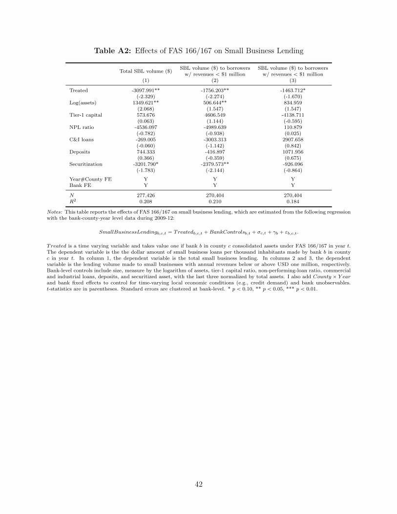
Table A2: Effects of FAS 166/167 on Small Business Lending

Total SBL volume ($)SBL volume ($) to borrowers SBL volume ($) to borrowers

w/ revenues ă $1 million w/ revenues ă $1 million(1) (2) (3)

Treated -3097.991** -1756.203** -1463.712*(-2.329) (-2.274) (-1.670)

Log(assets) 1349.621** 506.644** 834.959(2.068) (1.547) (1.547)

Tier-1 capital 573.676 4606.549 -4138.711(0.063) (1.144) (-0.595)

NPL ratio -4536.097 -4989.639 110.879(-0.782) (-0.938) (0.025)

C&I loans -269.005 -3003.313 2907.658(-0.060) (-1.142) (0.842)

Deposits 744.333 -416.897 1071.956(0.366) (-0.359) (0.675)

Securitization -3201.790* -2379.573** -926.096(-1.783) (-2.144) (-0.864)

Year#County FE Y Y YBank FE Y Y Y

N 277,426 270,404 270,404R2 0.208 0.210 0.184

Notes: This table reports the effects of FAS 166/167 on small business lending, which are estimated from the following regressionwith the bank-county-year level data during 2009-12:

SmallBusinessLendingb,c,t “ Treatedb,c,t `BankControlsb,t ` σc,t ` γb ` εb,c,t.

T reated is a time varying variable and takes value one if bank b in county c consolidated assets under FAS 166/167 in year t.The dependent variable is the the dollar amount of small business loans per thousand inhabitants made by bank b in countyc in year t. In column 1, the dependent variable is the total small business lending. In columns 2 and 3, the dependentvariable is the lending volume made to small businesses with annual revenues below or above USD one million, respectively.Bank-level controls include size, measure by the logarithm of assets, tier-1 capital ratio, non-performing-loan ratio, commercialand industrial loans, deposits, and securitized asset, with the last three normalized by total assets. I also add County ˆ Y earand bank fixed effects to control for time-varying local economic conditions (e.g., credit demand) and bank unobservables.t-statistics are in parentheses. Standard errors are clustered at bank-level. * p ă 0.10, ** p ă 0.05, *** p ă 0.01.

42

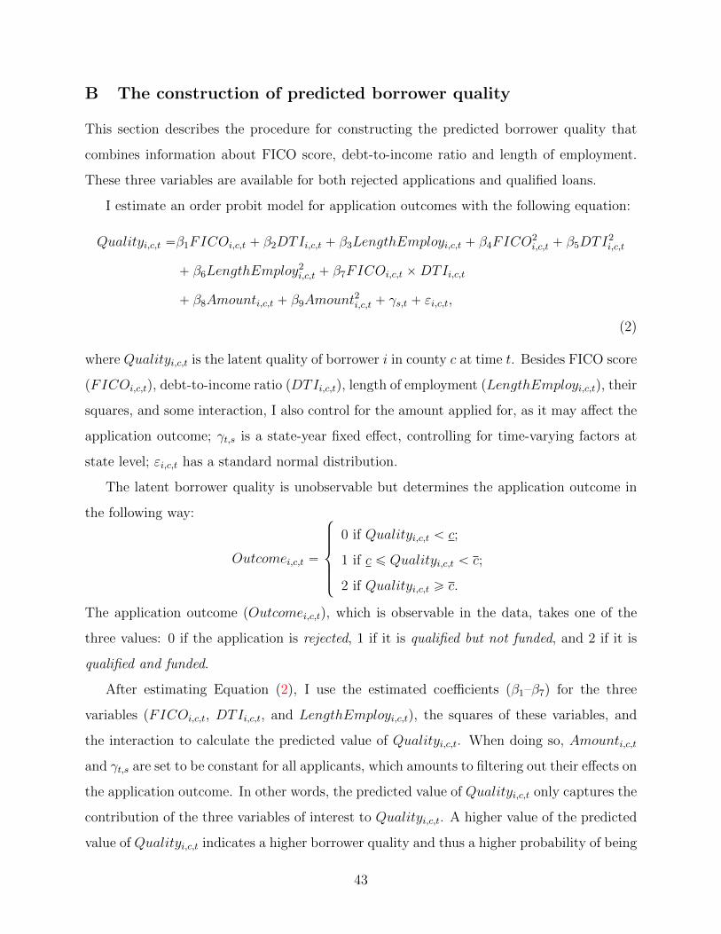
B The construction of predicted borrower quality

This section describes the procedure for constructing the predicted borrower quality that

combines information about FICO score, debt-to-income ratio and length of employment.

These three variables are available for both rejected applications and qualified loans.

I estimate an order probit model for application outcomes with the following equation:

Qualityi,c,t “β1FICOi,c,t ` β2DTIi,c,t ` β3LengthEmployi,c,t ` β4FICO2i,c,t ` β5DTI

2i,c,t

` β6LengthEmploy2i,c,t ` β7FICOi,c,t ˆDTIi,c,t

` β8Amounti,c,t ` β9Amount2i,c,t ` γs,t ` εi,c,t,

(2)

where Qualityi,c,t is the latent quality of borrower i in county c at time t. Besides FICO score

(FICOi,c,t), debt-to-income ratio (DTIi,c,t), length of employment (LengthEmployi,c,t), their

squares, and some interaction, I also control for the amount applied for, as it may affect the

application outcome; γt,s is a state-year fixed effect, controlling for time-varying factors at

state level; εi,c,t has a standard normal distribution.

The latent borrower quality is unobservable but determines the application outcome in

the following way:

Outcomei,c,t “

$

’

’

’

&

’

’

’

%

0 if Qualityi,c,t ă c;

1 if c ď Qualityi,c,t ă c;

2 if Qualityi,c,t ě c.

The application outcome (Outcomei,c,t), which is observable in the data, takes one of the

three values: 0 if the application is rejected, 1 if it is qualified but not funded, and 2 if it is

qualified and funded.

After estimating Equation (2), I use the estimated coefficients (β1–β7) for the three

variables (FICOi,c,t, DTIi,c,t, and LengthEmployi,c,t), the squares of these variables, and

the interaction to calculate the predicted value of Qualityi,c,t. When doing so, Amounti,c,t

and γt,s are set to be constant for all applicants, which amounts to filtering out their effects on

the application outcome. In other words, the predicted value of Qualityi,c,t only captures the

contribution of the three variables of interest to Qualityi,c,t. A higher value of the predicted

value of Qualityi,c,t indicates a higher borrower quality and thus a higher probability of being

43

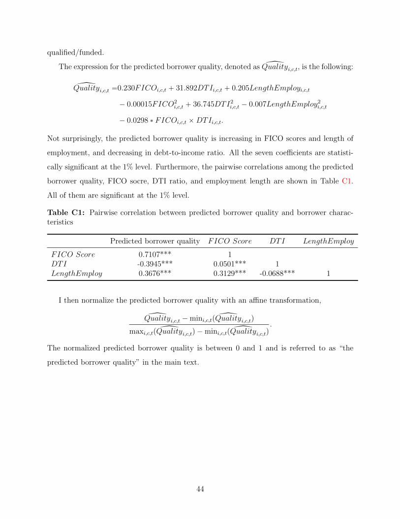
qualified/funded.

The expression for the predicted borrower quality, denoted as {Qualityi,c,t, is the following:

{Qualityi,c,t “0.230FICOi,c,t ` 31.892DTIi,c,t ` 0.205LengthEmployi,c,t

´ 0.00015FICO2i,c,t ` 36.745DTI2

i,c,t ´ 0.007LengthEmploy2i,c,t

´ 0.0298 ˚ FICOi,c,t ˆDTIi,c,t.

Not surprisingly, the predicted borrower quality is increasing in FICO scores and length of

employment, and decreasing in debt-to-income ratio. All the seven coefficients are statisti-

cally significant at the 1% level. Furthermore, the pairwise correlations among the predicted

borrower quality, FICO socre, DTI ratio, and employment length are shown in Table C1.

All of them are significant at the 1% level.

Table C1: Pairwise correlation between predicted borrower quality and borrower charac-teristics

Predicted borrower quality FICO Score DTI LengthEmploy

FICO Score 0.7107*** 1DTI -0.3945*** 0.0501*** 1LengthEmploy 0.3676*** 0.3129*** -0.0688*** 1

I then normalize the predicted borrower quality with an affine transformation,

{Qualityi,c,t ´mini,c,tp {Qualityi,c,tq

maxi,c,tp {Qualityi,c,tq ´mini,c,tp {Qualityi,c,tq.

The normalized predicted borrower quality is between 0 and 1 and is referred to as “the

predicted borrower quality” in the main text.

44