Pedagogical Review of Quantum Measurement Theory with an

Pedagogical Review ofQuantum Measurement Theorywith an Emphasis onWeak MeasurementsBengt E. Y. Svensson

Department of Astronomy and Theoretical Physics, Lund University, Sweden. E-mail: Bengt E [email protected]

Editors: Danko Georgiev & Stefano Ansoldi

Article history: Submitted on January 25, 2013; Accepted on April 30, 2013; Published on May 15, 2013.

The quantum theory of measurement has beenwith us since quantum mechanics was invented.It has recently been invigorated, partly due to

the increasing interest in quantum information sci-ence. In this partly pedagogical review I attemptto give a self-contained overview of non-relativisticquantum theory of measurement expressed in densitymatrix formalism. I will not dwell on the applicationsin quantum information theory; it is well covered byseveral books in that field. The focus is instead on ap-plications to the theory of weak measurement, as de-veloped by Aharonov and collaborators. Their devel-opment of weak measurement combined with whatthey call post-selection – judiciously choosing not onlythe initial state of a system (pre-selection) but also itsfinal state – has received much attention recently. Notthe least has it opened up new, fruitful experimen-tal vistas, like novel approaches to amplification. Butthe approach has also attached to it some air of mys-tery. I will attempt to demystify it by showing that (al-most) all results can be derived in a straight-forwardway from conventional quantum mechanics. Amongother things, I develop the formalism not only to firstorder but also to second order in the weak interac-tion responsible for the measurement. I apply it tothe so called Leggett–Garg inequalities, also knownas Bell inequalities in time. I also give an outline, evenif rough, of some of the ingenious experiments that

the work by Aharonov and collaborators has inspired.As an application of weak measurement, not relatedto the approach by Aharonov and collaborators, theformalism also allows me to derive the master equa-tion for the density matrix of an open system in inter-action with an environment. An issue that remains inthe weak measurement plus post-selection approachis the interpretation of the so called weak value of anobservable. Is it a bona fide property of the systemconsidered? I have no definite answer to this ques-tion; I shall only exhibit the consequences of the pro-posed interpretation.Quanta 2013; 2: 18–49.

1 Introduction

The measurement aspects of quantum mechanics are asold as quantum mechanics itself. When von Neumannwrote his overview [1] of quantum mechanics in 1932, hecovered several of these aspects. The review volume [2]edited by Wheeler and Zurek tells the history up until1983. Since then, the interest has if anything increased,

This is an open access article distributed under the termsof the Creative Commons Attribution License CC-BY-3.0, whichpermits unrestricted use, distribution, and reproduction in any medium,provided the original author and source are credited.

Quanta | DOI: 10.12743/quanta.v2i1.12 May 2013 | Volume 2 | Issue 1 | Page 18

mailto:[email protected]

http://creativecommons.org/licenses/by/3.0/

http://dx.doi.org/10.12743/quanta.v2i1.12

in particular in connection with the growth of quantuminformation science. Three books reflect the evolutionof the field: the one by Braginsky and Khalili [3] from1992, the one by Nielsen and Chuang [4] from 2000,and the more recent one by Wiseman and Milburn [5]from 2009. One important feature in the developmentover the last decades has been the increasing emphasis onwhat is call ancilla (or indirect) measurement, in whichthe measurement process is modeled in some detail byconsidering how the system under study interacts withthe measurement device.

Since the seminal paper [6] from 1988 by Aharonov,Albert and Vaidman, there has been another interestingdevelopment largely parallel to other ones. This is thefield of weak measurement and weak values. Since itwas started, its ideas have been skillfully advocated, inparticular by Aharonov and collaborators; see [7–17]. Athorough, up-to-date review of the field with an extensivelist of references is in [18].

Aharonov and collaborators started from the well-known characteristics of quantum mechanics which dis-tinguishes it from classical physic: a quantum mechanicalmeasurement irrevocably disturbs the system measured.What, they asked, would happen if the interaction respon-sible for the measurement becomes very weak? True, thedisturbance will decrease but so will also the informationobtained in the measurement process. The revolutionaryobservation by Aharonov and collaborators is that thistrade-off could be to the advantage of the non-disturbanceaspect. There is new physics to be extracted from weakmeasurement, in particular when the weak measurementis combined with a judicious choice of the initial state(pre-selection) and the final state (post-selection) of thesystem under study.

This article provides an overview of the field of weakmeasurement without claiming originality of the results.The purpose is also to give a general pedagogical intro-duction to some more modern aspects of quantum theoryof measurement. Prerequisites from readers will onlybe basic knowledge of the standard formulation of quan-tum mechanics in Hilbert space as presented in any well-written textbook on quantum mechanics, like [19,20]; thelatter also covers some of the material I present in thisarticle.

To make the article self-contained, and to introducethe notations to be used, I begin anyhow with a summaryof the standard quantum theory of measurement. In sec-tion 2, I treat the direct (or projective) scheme, and insection 3 and section 4, the indirect (or ancilla) scheme. Ido this in the density matrix formalism, which I also de-scribe in some detail; other names for the density matrixare state matrix, density operator and statistical operator.Part of my motivation for doing so is that this formalism –

arguably slightly more general than the pure-state, wave-function (or Hilbert-space state) formalism – is a straight-forward, though maybe somewhat clumsy, approach toreaching the quantum mechanical results one wants, andthis, again arguably, in a less error-prone way. In fact,the density matrix formalism provides an indispensabletool for any thorough-going analysis of the measurementprocess. Despite my preference for density matrices, insome of the more concrete problems I revert to the pure-state formalism. Anyhow, I illustrate in subsection 10.2the advantage of the density matrix formalism by a sidetheme, not related to the main track of the article, viz.,continuous measurement. In particular I derive, even ifin a pedestrian way, the so called master equation for anopen system.

The approach to the measurement process taken hereis not the most general one. An approach based onso called measurement operators and on effects, aliaspositive-operator valued measures (POVMs) is more gen-eral; see [5, section 1.4.1] and subsection 10.1. In fact, thebasic premises of that approach can be derived from thedensity matrix treatment of the ancilla method reviewedin section 3. In subsection 10.1, I expose these items.

In section 5, my treatment of weak measurements willbe focused on the scheme by Aharonov and collabora-tors that combines it with post-selection. I present themain arguments and derive expressions for the relevantquantities. In fact, I do this not only to linear order in thestrength of the interaction but to second order.

Even without invoking weak measurements, it is ofinterest to study amplification. This is done by focusingon that subensemble of the total measured sample thatarises from chosing only those events that end up in aparticular final state. I give some examples on how suchan amplification setup could be implemented.

If there ever were any magic connected with the deriva-tion and application of weak value, I hope my presentationwill get rid of them. For example, nowhere in my argu-ments will there occur negative probabilities or complexvalues of a number operator. In fact, what I present isnothing but conventional quantum mechanics applied tosome particular problems. In short, I hope that the articlewill provide a framework that aims to clear up some ofthe inadvertencies regarding the concept of weak valuethat, in my opinion, can be found in the literature both bytheorists and experimentalists.

In section 6, I choose to illustrate the fruitfulness ofthe weak measurement plus post-selection approach byapplying it to the so called Leggett–Garg inequalities [21],sometimes also called the Bell inequalities in time.

In section 7, I describe, even if in rough outlines only,some of the very ingenious experiments – admittedlysubjectively chosen – that have exploited the new vistas



opened up by the weak measurement plus post-selectionapproach. To give a trailer of what they include: it isnowadays possible to measure the wave function of aparticle directly, as well as to map the trajectories of theparticles in a double-slit setup.

Up till the last but one section of this article, the argu-ments are strictly based on conventional quantum mechan-ics and should not meet with any objections. If there areany open questions regarding the approach by Aharonovand collaborators, they concern the very interpretation ofthe formalism. In section 8, I venture into this slightlycontroversial field. There, I attempt to further illuminatesome of the basic premises that underlie the concept of aweak value, but also to raise some questions regarding itsmeaning and interpretation.

A final section 9 before the appendices gives a sum-mary and some further discussion of the conclusionsreached in the article.

Not covered in this article is the extension of conven-tional quantum mechanics in terms of the so called thetwo-state vector formalism that Aharonov and collabora-tors have proposed [7], partly as a further development oftheir weak measurement approach. These ideas definitelygo beyond conventional quantum mechanics. Anotheractive field of research, which is not covered herein, is theinformation-theoretic aspect of the quantum measurementprocess. Here, I may refer the interested reader to [4, 5].

2 The ideal (or projective)measurement scheme

2.1 The basic scheme

All treatment of measurements in conventional quantummechanics relies in one way or another on a standardtreatment of the measurement process due to Born andvon Neumann [1], with later extension by Luders [22].The scheme is sometimes also named after von Neumann.Since I will refer to a von Neumann protocol later on inthis article, I prefer not to attach von Neumann’s nameto the present scheme in order not to cause unnecessaryconfusion.

As it is described in most textbooks, it goes somethinglike this. The object to be measured is a system S de-scribed by a normalized ket |s〉 in a (finite-dimensional)Hilbert spaceHS. This system could be an atom, an elec-tron, a photon, or anything amenable to a quantum me-chanical description. Suppose we are interested in mea-suring an observable S on this system. The observable isdescribed by a Hermitian operator S = S † and has a com-plete, orthonormal set of eigenstates |si〉, i = 1, 2, . . . , dS ,where dS is the dimension of the Hilbert spaceHS.

The physical interpretation is entailed in the followingrules:

Rule (1): The possible result of measuring the observ-able S on the system S is one of the eigenvalues si of theoperator S , and nothing else.

Rule (2): Under the same conditions, the probabilityof obtaining a particular eigenvalue si (assumed for sim-plicity to be non-degenerate) of the operator S , given thatthe system S is in the state |s〉, is

prob(si||s〉) = |〈si|s〉|2 (1)

Rule (3): After such a measurement with the result si,the system S is described by the ket |si〉. This is usuallydescribed as the reduction (or collapse) of the state vector|s〉 to |si〉.

Moreover, I shall only consider non-destructive mea-surements, i.e., measurements that do not destroy thesystem, even if they may leave it in a new state. For ex-ample, if the system is a photon, I require there still to bea photon after the measurement.

Let me elaborate somewhat on these basic premises.Firstly, I want to reformulate the postulates in the more

general framework, where states are described by densitymatrices, also called density operators or statistical oper-ators. These are not vectors but operators in the Hilbertspace HS. For the simple case when the system S isdescribed by a pure state in the form of a ket

|s〉 =

dS∑i=1

ci|si〉 (2)

the corresponding density matrix – I will denote it by σ –is simply the projector Ps with the definition

σ = Ps = |s〉〈s| (3)

In the more general case, when the system S is describedby a (classical) statistical mixture, i.e., an incoherentsuperposition of pure, normalized (but not necessarilyorthogonal) states |s(a)〉, a = 1, 2, . . . ,K, each with itsprojector Ps(a) and each with a probability pa, the densitymatrix σ representing the state of the system S is givenby

σ0 =

K∑a=1

paPs(a) (4)

Here, I attached a subscript 0 to σ in order to identify itas the initial state. We shall meet such density matricesin a slightly different context later on, when discussingthe state of one part of a system composed of severalsubsystems.

One important property of a density matrix is that ithas unit trace, the trace being defined as the sum of its



diagonal elements

Tr(σ0) =

K∑a=1

paTr(Ps(a)

)=

K∑a=1

pa = 1 (5)

This trace property of any density matrix then expressesthe normalization condition and is a very useful checkwhen performing calculations.

With such an incoherent sum of pure states, the threemeasurement rules above take a partly new form:

Rule (1′): Same as rule (1).Rule (2′): The probability of obtaining a particular

eigenvalue si of the operator S , given that the system Sis in the state σ0, is

prob (si|σ0) =∑

a

paprob(si||s(a)〉

)(6)

Before turning to the third (collapse) condition in thedensity matrix formalism, I want to elaborate on this newexpression for the probability. Using

prob(si||s(a)〉

)= |〈si|s(a)〉|2

= 〈si|s(a)〉〈s(a)|si〉

= 〈si|Ps(a) |si〉 (7)

one finds

prob (si|σ0) = 〈si|∑

a

paPs(a) |si〉

= 〈si|σ0|si〉 (8)

It is standard to rewrite this simple expression in a slightlymore complicated form, which will be advantageous lateron. Using the fact that the eigenstates are orthogonal,〈si|s j〉 = δi, j, one deduces that

prob (si|σ0) = 〈si|σ0|si〉

=∑

j

〈s j|si〉〈si|σ0|si〉〈si|s j〉

= Tr(Psiσ0Psi

)= Tr

(Psiσ0

)(9)

Here the last equation follows from the easily provedinvariance of the trace under cyclic permutations andfrom the fact that a projector P is idempotent

PP = P2 = P (10)

As an interim summary, then, the second condition maybe formulated as:

Rule (2′): The probability of obtaining a particulareigenvalue si of the operator S , given that the system Sis in the state σ0, is

prob (si|σ0) = Tr(Psiσ0

)(11)

The collapse condition may now be stated in two dif-ferent forms, as conditional or unconditional. The con-ditional (or ‘selective’) form applies when one asks forthe density matrix after the measurement with a particularresult si and reads:

Rule (3′): Measurement of S , with result si, transformsthe original density matrix σ0 into the conditional densitymatrix σ1(hereafter subscript 1 identifies entities after themeasurement) according to

σ0 →Psiσ0Psi

prob(si|σ0)= σ1(|si) (12)

This is the so called Luders’ rule [22] for how an idealmeasurement transforms (or collapses or updates) theinitial density matrix; we will meet this rule in severaldisguises in the sequel.

Let me note in passing that the rules (2′) and (3′) in factalso apply in case the eigenvalue si is degenerate, thenwith the projector onto a non-degenerate state replacedby the projector onto that subspace of the Hilbert spaceHS which is spanned by the eigenvectors having thiseigenvalue.

It is easy to check that the rule (3′) entails the rule(3) when the density matrix σ0 represents a pure state.Moreover, one may convince oneself that the conditionaldensity matrix, σ1(|si), even if the initial state is a mixture,represents a pure state provided the eigenvalue si is non-degenerate.

The unconditional or non-selective case occurs whenthe measurement is performed but when, for one reasonor another, one does not register the outcomes. Then,one must average over the possible conditional densitymatrices, each with its probability, to get:

Rule (3′′): Measurement of S , but without registeringthe result, transforms the original density matrix σ0 intothe unconditional density matrix σ1 according to

σ0 →∑

i

prob(si|σ0)σ1(|si)

=∑

i

(Psiσ0Psi

)= σ1 (13)

2.2 Post-selection and theAharonov–Bergmann–Lebowitz rule

As an application of the projective measurement scheme,let me consider a situation in which two successive mea-surements are made on the same system; remember that Isuppose all measurement on the system under study to benon-destructive.

Begin by preparing (pre-selecting) the system S in aninitial (pure, for simplicity) state |s〉. Let this be followedby a measurement of the observable S , resulting in one



|s>

|s1>

|s2>

|s3>

|si>

|sds>

|f>

S F

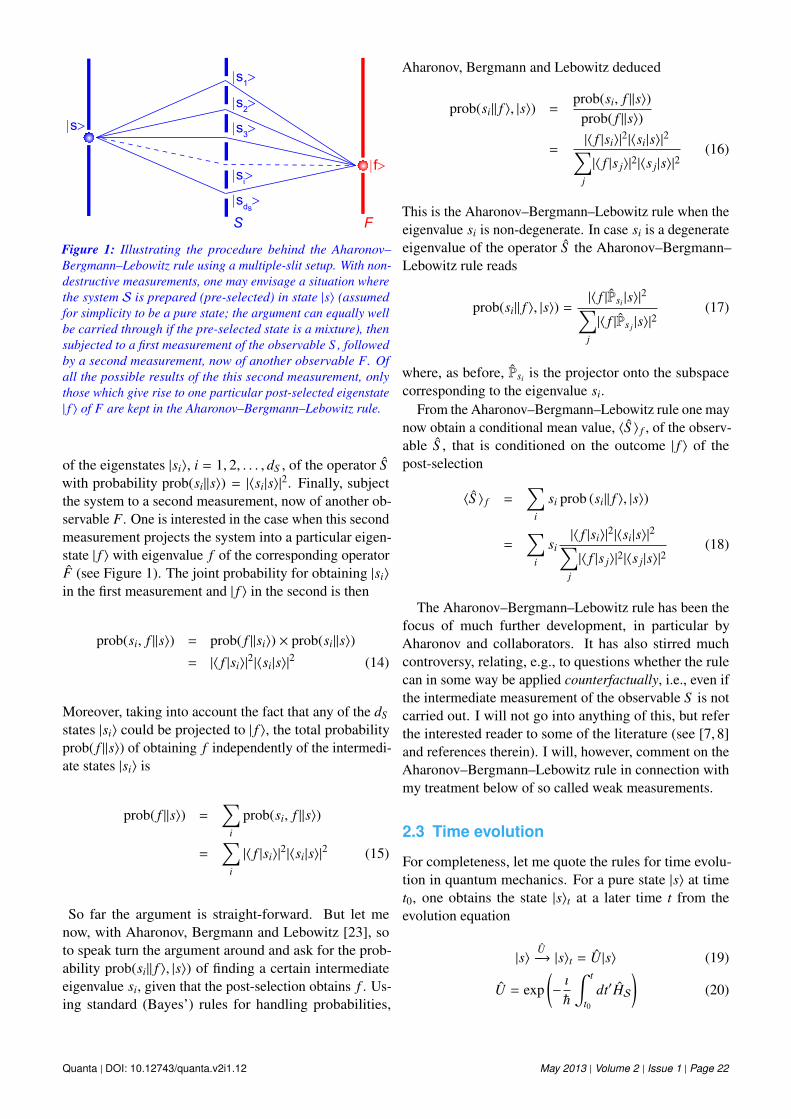
Figure 1: Illustrating the procedure behind the Aharonov–Bergmann–Lebowitz rule using a multiple-slit setup. With non-destructive measurements, one may envisage a situation wherethe system S is prepared (pre-selected) in state |s〉 (assumedfor simplicity to be a pure state; the argument can equally wellbe carried through if the pre-selected state is a mixture), thensubjected to a first measurement of the observable S , followedby a second measurement, now of another observable F. Ofall the possible results of the this second measurement, onlythose which give rise to one particular post-selected eigenstate| f 〉 of F are kept in the Aharonov–Bergmann–Lebowitz rule.

of the eigenstates |si〉, i = 1, 2, . . . , dS , of the operator Swith probability prob(si||s〉) = |〈si|s〉|2. Finally, subjectthe system to a second measurement, now of another ob-servable F. One is interested in the case when this secondmeasurement projects the system into a particular eigen-state | f 〉 with eigenvalue f of the corresponding operatorF (see Figure 1). The joint probability for obtaining |si〉

in the first measurement and | f 〉 in the second is then

prob(si, f ||s〉) = prob( f ||si〉) × prob(si||s〉)

= |〈 f |si〉|2|〈si|s〉|2 (14)

Moreover, taking into account the fact that any of the dS

states |si〉 could be projected to | f 〉, the total probabilityprob( f ||s〉) of obtaining f independently of the intermedi-ate states |si〉 is

prob( f ||s〉) =∑

i

prob(si, f ||s〉)

=∑

i

|〈 f |si〉|2|〈si|s〉|2 (15)

So far the argument is straight-forward. But let menow, with Aharonov, Bergmann and Lebowitz [23], soto speak turn the argument around and ask for the prob-ability prob(si|| f 〉, |s〉) of finding a certain intermediateeigenvalue si, given that the post-selection obtains f . Us-ing standard (Bayes’) rules for handling probabilities,

Aharonov, Bergmann and Lebowitz deduced

prob(si|| f 〉, |s〉) =prob(si, f ||s〉)

prob( f ||s〉)

=|〈 f |si〉|

2|〈si|s〉|2∑j

|〈 f |s j〉|2|〈s j|s〉|2

(16)

This is the Aharonov–Bergmann–Lebowitz rule when theeigenvalue si is non-degenerate. In case si is a degenerateeigenvalue of the operator S the Aharonov–Bergmann–Lebowitz rule reads

prob(si|| f 〉, |s〉) =|〈 f |Psi |s〉|

2∑j

|〈 f |Ps j |s〉|2(17)

where, as before, Psi is the projector onto the subspacecorresponding to the eigenvalue si.

From the Aharonov–Bergmann–Lebowitz rule one maynow obtain a conditional mean value, 〈S 〉 f , of the observ-able S , that is conditioned on the outcome | f 〉 of thepost-selection

〈S 〉 f =∑

i

si prob (si|| f 〉, |s〉)

=∑

i

si|〈 f |si〉|

2|〈si|s〉|2∑j

|〈 f |s j〉|2|〈s j|s〉|2

(18)

The Aharonov–Bergmann–Lebowitz rule has been thefocus of much further development, in particular byAharonov and collaborators. It has also stirred muchcontroversy, relating, e.g., to questions whether the rulecan in some way be applied counterfactually, i.e., even ifthe intermediate measurement of the observable S is notcarried out. I will not go into anything of this, but referthe interested reader to some of the literature (see [7, 8]and references therein). I will, however, comment on theAharonov–Bergmann–Lebowitz rule in connection withmy treatment below of so called weak measurements.

2.3 Time evolution

For completeness, let me quote the rules for time evolu-tion in quantum mechanics. For a pure state |s〉 at timet0, one obtains the state |s〉t at a later time t from theevolution equation

|s〉U−→ |s〉t = U |s〉 (19)

U = exp(−ı

~

∫ t

t0dt′HS

)(20)



by time-integration of the Schrodinger equation with theHamiltonian HS. This translates immediately to the timeevolution of a density matrix

σ0 → σt = Uσ0U† (21)

with U† the Hermitian conjugate of U.

3 The indirect (or ancilla)measurement scheme

3.1 Modeling the measurement process

The approach to measurement described in section 2leaves the concept of measurement unanalyzed. In partic-ular, it takes no account whatsoever of how the measure-ment is performed, what kind of measurement apparatusis used, what distinguishes measurements from other pos-sible types of interactions, etc.

In the indirect, or ancilla, scheme that I will now de-scribe, one goes a few steps in the direction of describ-ing the very measurement process. True, it is still veryschematic. But at least it introduces a measurement de-vice (or ancilla) – to be alternatively called a meter or apointer – into the picture even if ever so schematically.It is the interaction of the meter with the system – calledalternatively the object, or the probe or, for photons, thesignal photon – that constitute the measurement: by read-ing off the meter one gets information as to the value ofthe system observable. Note that in experimental situa-tions, the meter and the system could even be propertiesof one and the same physical object – like momentumand polarization for a photon (see section 7 for someexamples).

The meterM will be modeled as a quantum device. Ithas a Hilbert space HM with a complete, orthonormalset of basis states |mk〉, k = 1, 2, . . . , dM, where dM isthe dimension of HM. The operator in HM which hasthese states as eigenstates is denoted M. For reasons tobecome clearer later on, the observable M is called thepointer variable, and the states |mk〉 the pointer states.The intrinsic Hamiltonian ofM is denoted HM. For sim-plicity, it will be assumed to vanish in most cases I treat– if not, use time-dependent operators in the Heisenbergrepresentation (see [24]) – but it is instructive to keep itwhen setting up the scheme. Projectors in HM will bedenoted Omk , etc. The meter is assumed to be prepared inan initial pure state |m(0)〉 – not necessarily an eigenstateof the pointer variable M (see below) – so that the meterinitial density matrix is µ0 = |m(0)〉〈m(0)|.

The object or system S – I sometimes also refer to it asthe object-system in order to distinguish it from the totalsystem comprising the meter and the object-system – has

its Hilbert spaceHS in the same way as in the projectivemeasurement scheme of section 2. It has a complete,orthonormal set of basis states |si〉, i = 1, 2, . . . , dS , withdS the dimension of the Hilbert space HS. They areeigenstates of the operator S inHS which corresponds tothe observable S to be measured. The system’s intrinsicHamiltonian is HS (which, as with HM, I will assume tovanish); projectors in HS will be denoted Psi , etc. Thesystem is assumed to be initially prepared (pre-selected)either in a pure state |s〉 given by Equation 2 – in whichcase its density matrix is σ0 = |s〉〈s| – or in a moregeneral state described by an arbitrary σ0 (but of coursenormalized so that Tr(σ0) = 1).

The total system T comprises the object-system S andthe meterM. Its Hilbert space isHT = HS⊗HM, wherethe symbol ⊗ stands for the direct product. The initialstate of the total system is τ0 = σ0 ⊗ µ0, i.e. the systemand the meter are assumed to be initially uncorrelated(not entangled). The total Hamiltonian is

HT = HS + HM + Hint (22)

The interaction Hamiltonian Hint does not vanish, anddepends on the observable S to be measured as well as ona pointer variable; see below for details. Moreover, theassumption of non-destructive measurement (as spelledout in subsection 3.2 below) – in the present case, withvanishing intrinsic Hamiltonians, this is the criterion for aso called quantum non-demolition measurement – impliesthat the commutator [Hint, S ] = 0.

3.2 The pre-measurement

The system and the meter are assumed to interact via aunitary time-evolution operator U in what is called a pre-measurement. This means that the total system T withits initial density matrix τ0 will evolve unitarily into τ1:

τ0 = σ0 ⊗ µ0U−→ τ1 = Uσ0 ⊗ µ0U† (23)

where U† is the Hermitian conjugate of U. If the Hamil-tonian is known, the unitary operator U is given by

U = exp(−ı

~

∫dtHT

)(24)

with t denoting time. To start with, I shall, however, notuse this Hamiltonian expression but characterize U inanother way.

To this end, note that for U to be a pre-measurementof S , U must have properties so that it distinguishes be-tween the different states |si〉. It is therefore assumedthat an initial joint pure state |si〉 ⊗ |m(0)〉 of the system



and the meter – remember that I consider non-destructivemeasurements – is transformed by U into

|si〉 ⊗ |m(0)〉U−→ U

(|si〉 ⊗ |m(0)〉

)= |si〉 ⊗ |m(i)〉 (25)

where i = 1, 2, . . . , dS and the meter states |m(i)〉 act asmarkers for the system state |si〉; we will see in detail howthis comes about later.

If this initial state is a superposition of eigenstates givenby Equation 2, and because U is a linear operator, we get

|s〉 ⊗ |m(0)〉U−→ U

(|s〉 ⊗ |m(0)〉

)=

dS∑i=1

ci|si〉 ⊗ |m(i)〉 (26)

The joint matrix τ0 = σ0 ⊗ µ0, written out in full detail,evolves according to

τ0U−→ τ1 = Uσ0 ⊗ µ0U†

=∑i, j

(|si〉 ⊗ |m(i)〉〈si|σ0|s j〉〈s j| ⊗ 〈m( j)|

)=

∑i, j

(|m(i)〉Psiσ0Ps j〈m

( j)|)

(27)

where the last equation has introduced the projectionoperators Psi = |si〉〈si| and similarly for Ps j .

It is important to note that

• A system’s pure eigenstate |si〉 is left unchanged un-der this operation; among other things, the assump-tion of a non-destructive measurement is importanthere.

• One of the most important consequences of the pre-measurement is that the object-system’s state be-comes correlated (entangled) with the meter state:τ1 cannot be written as a product of one object stateand one meter state.

• The meter states |m(0)〉 and |m(i)〉 are, in general, noteigenstates of the meter operator M, but superpo-sitions of such eigenstates. In particular, the states|m(0)〉 and |m(i)〉, i = 1, 2, . . . , dS , are normalized butin general not mutually orthogonal. Nor do theyform a complete set inHM. Indeed, the dimensionsdS and dM of the respective Hilbert spacesHS andHM need not be equal.

• The operation U thus correlates the system state|si〉 with the meter state |m(i)〉 but not necessarilyin a unique way: to each |si〉 there corresponds adefinite |m(i)〉, different for different |si〉, but therecould be overlap between |m(i)〉 and |m( j)〉, expressedby 〈m(i)|m( j)〉 , 0, for i , j. An example we willsee in more detail later on : |m(i)〉 could represent a

Gaussian distribution (Equation 42) for a continu-ous pointer variable q (the position of a pointer on ascale) so that |m(i)〉 ∼ exp

[−(q − gsi)2/4∆2

], where

g is a coupling constant and ∆ the width of the Gaus-sian; for large enough ∆ compared to gsi, differentwave functions (different i-values) will overlap sub-stantially. See further subsection 4.1 below.

The rule for obtaining the separate states σ1 for the sys-tem, and µ1 for the meter, after this pre-measurement, isto take the partial trace over the non-interesting degreesof freedom. In case we want the state σ1 of the system,this means summing over the basis states |mk〉 for HM,transforming an operator inHS ⊗HM into one inHS:

σ0U−→ σ1 = TrMτ1 =

∑k

〈mk|τ1|mk〉

=∑k,i, j

〈mk|m(i)〉Psiσ0Ps j〈m( j)|mk〉

=∑i, j

(Psiσ0Ps j〈m

( j)|m(i)〉)

(28)

The last equation follows from the completeness of thebasis states |mk〉 in the Hilbert spaceHM.

As is seen, were it not for a possible overlap betweenthe meter states |m(i)〉 and |m( j)〉, the system density matrixσ1 after the pre-measurement would have had diagonalelements only, i.e. would not have allowed any interfer-ence effects between different eigenvalues si. Anotherway to express this fact is to realize that, in case of nooverlap between different states |m(i)〉, the indirect mea-surement scheme have the same consequences for theobject-system as would a projective measurements havehad: if 〈m(i)|m( j)〉 = 0 for i , j, then the ancilla schemeis the same as the projective scheme. The general case,〈m(i)|m( j)〉 , 0 for i , j, does allow for interference, afact which will have interesting measureable effects aswe will see in more detail in section 5.

The same conclusion may be reached by consideringthe meter. Its state after the pre-measurement is

µ0U−→ µ1 = TrSτ1 =

∑i

〈si|τ1|si〉

=∑

i

|m(i)〉〈si|σ0|si〉〈m(i)| (29)

with matrix elements

〈mk|µ1|ml〉 =∑

i

〈mk|m(i)〉〈si|σ0|si〉〈m(i)|ml〉 (30)

expressed in terms of the wavefunctions 〈mk|m(i)〉. Fromthis result we again see clearly that a pre-measurementcan distinguish effectively between different values si

of the system observable S only if different meter wavefunctions 〈mk|m(i)〉 do not overlap.



3.3 The read-out: Projective measurementon the meter

So far, no real measurement has been performed in thesense of obtaining a record. The entangled system-meteris still in a quantum-mechanical superposition τ1. Oneneeds a recording, a read-out of the meter, in order toobtain information that constitutes a real measurement(see for example [5] , in particular section 1.2)

Therefore, the next step in this indirect measurementscheme is to subject the meter, and only the meter, toa projective measurement of the pointer observable M.Reading off the meter means obtaining an eigenvaluemk of the corresponding operator M in a reaction thatis symbolized by the projector Omk = |mk〉〈mk| onto thecorresponding subspace of the meter Hilbert spaceHM.Since, as a result of the pre-measurement, the system isentangled with the meter, this will influence the systemstate too, and is therefore also a measurement of theobject-system as will be evident shortly.

For the total density matrix, this projective measure-ment, complying to the Luders’ rule (Equation 12), im-plies

τ1Omk−−−→ τ1(|mk) =

(IS ⊗ Omk

)τ1

(IS ⊗ Omk

)prob (mk)

(31)

where IS is the unit operator inHS and where prob(mk) =

prob(mk|τ1) is the probability of obtaining the pointervalue mk given the state τ1. It may be evaluated

prob(mk) = TrT[(IS ⊗ Omk

)τ1

]=

∑i

(|〈m(i)|mk〉|

2〈si|σ0|si〉)

=∑

i

prob(mk||m(i)〉) × prob(si|σ0) (32)

Note again that the mk-distribution reflects the si-distribution uniquely only if the different wave functions〈mk|m(i)〉 do not overlap.

The result for prob(mk) may seem remarkable: noquantum-mechanical interference here! Rather, the prob-ability of finding the value mk for the pointer variableis the sum of products of two probabilities. The one isprob(mk||m(i)〉), the probability to obtain the pointer valuemk, given the state |m(i)〉 that corresponds, in the pre-measurement, to the state |si〉. The other is prob(si|σ0),the probability to obtain the value si in the initial stateσ0 of the system. Indeed this is what one would expectfrom a pure classical treatment of probabilities, but hereit arises from the quantum mechanical formalism.

So what have we learned concerning the object-systemfrom this read-out of the meter? The answer sits in itsdensity matrix σ1(|mk) after the read-out, representing

as it does the state of the system after that action. It isobtained in the usual way by taking the partial trace ofthe corresponding total density matrix

σ1(|mk) = TrMτ1(|mk)

=1

prob(mk)TrM

[(IS ⊗ Omk

)τ1

(IS ⊗ Omk

)]=

1prob(mk)

〈mk|Uσ0 ⊗ µ0U†|mk〉

=1

prob(mk)〈mk|U |m(0)〉σ0〈m(0)|U†|mk〉

=1

prob(mk)Ωkσ0Ω

†

k (33)

where Ωk is an operator onHS defined by

Ωk = 〈mk|U |m(0)〉

=∑

i

〈mk|m(i)〉|si〉〈si|

=∑

i

〈mk|m(i)〉Psi (34)

The operators Ωk are called measurement operators,in the literature often denoted Mk (but I use Ωk since inthis article I use M for entities related to the meter). Theyplay an important role in general theories of measure-ment [4, 5]. Some of their properties are presented insubsection 10.1.

If we, in describing the system after the pre-measurement, do not care which of the results mk is ob-tained in the projective measurement on the meter – wedeliberately neglect the outcome of the read-out – thenthe system must be described by the statistical sum overall possibilities∑

k

prob(mk) × σ1(|mk) =∑

k

Ωkσ0Ω†

k

=∑

k

〈mk|Uσ0 ⊗ µ0U†|mk〉 = σ1 (35)

This is exactly the same unconditional density matrixσ1, Equation 28, as the one that describes the systemright after the pre-measurement and before the projec-tive measurement of the meter has taken place. For thisunconditional density matrix of the system it is thus ofno importance whether one performs the projective mea-surement on the meter or not, provided the result is notrecorded. In particular, an unregistered projective metermeasurement has no effect on the probability distributionfor the eigenvalues si.

For completeness, I also give the meter’s density matrixafter the meter has been read-out. It takes the form

µ1(|mk) =Omk µ1Omk

prob(mk)(36)



In particular, the meter and the object-system becomeun-entangled after a conditional measurement (but notafter an unconditional one).

Now that the machinery is set up, it may be used toanswer any legitimate question regarding results of themeasurement process. I will use it extensively in thesequel. But first, I will need a further general result.

3.4 Consecutive measurements

For future use, I will consider the case of two succes-sive ancilla measurements. The system remains intact –remember I require non-destructive measurement – butis transformed in steps according to the rules just estab-lished.

To start with, let me assume that the second measure-ment involves a different meter from the first. Lookingonly at the un-conditional matrices for the system, onehas

σ01st measurement−−−−−−−−−−−−→ σ1 =

∑k1

Ω(1)k1σ0Ω

(1)†k1

σ12nd measurement−−−−−−−−−−−−→ σ2 =

∑k2

Ω(2)k2σ1Ω

(2)†k2

(37)

σ2 =∑k1,k2

Ω(2)k2

Ω(1)k1σ0Ω

(1)†k1

Ω(2)†k2

=∑k1,k2

Ω(2)k2

Ω(1)k1σ0

(Ω

(2)k1

Ω(1)k2

)†(38)

That is, the measurement operators for consecutive ancillameasurement compose naturally. In particular, the gener-alization to any number of consecutive measurements isobvious.

If the second measurement is identical – has an identi-cal meter to the first and is involved in an identical unitarypre-measurement U as the first – the expression simplifiesto

σ2 =∑k,k′

Ω(1)k′ Ω

(1)k σ0

(Ω

(1)k′ Ω

(1)k

)†=

∑i, j

Psiσ0Ps j

(〈m( j)|m(i)〉

)2(39)

as is seen by a short calculation. This expression, too, iseasily generalized to any number of identical measure-ments.

4 Some application of the ancillascheme

In this section, I give some examples of applications(protocols) based on the indirect, or ancilla, measurement

scheme. These examples will be used several times lateron in the article for more concrete illustration of particularaspects of weak measurements and weak values.

4.1 The von Neumann protocol

Soon after quantum mechanics was invented, von Neu-mann [1, chapter 6] gave a formulation of the measure-ment process which is, essentially, a specific applicationof the ancilla scheme. His protocol gives a more detailedspecification of the meterM and uses a particular formfor the interaction Hamiltonian Hint between the object-system S and the meter M and, consequently, for theunitary pre-measurement operator U. I will now describethat measurement protocol, for simplicity for the casewhere the initial state is a pure state.

As a matter of terminology, do not confuse the vonNeumann measurement protocol presented here, whichis a particular realization of the present ancilla measure-ment scheme, with the von Neumann scheme, which is aterm sometimes used as alternative name to the projectivemeasurement scheme described in section 2.

The meter is supposed to have a continuous pointervariable Q replacing M, and with pointer states |q〉 replac-ing |mk〉. Here, I take the usual liberty of the physicistin translating, without further ado, a discrete treatmentin the finite-dimensional Hilbert space HM into a con-tinuous one. Almost realistically, q is to be thought ofas the pointer position of a graded gauge. One may thenintroduce the wave functions ϕ0(q) and ϕi(q) from theexpansions

|m(0)〉 =

∫dq|q〉〈q|m(0)〉 =

∫dq|q〉ϕ0(q) (40)

|m(i)〉 =

∫dq|q〉〈q|m(i)〉 =

∫dq|q〉ϕi(q) (41)

I shall assume that the initial pointer state ϕ0(q) iscentered around q = 0, i.e., that the expectation value〈Q〉0 in the initial state vanishes. A particular choice forϕ0(q) could be

ϕ0(q) =

[1

√2π∆2

exp(−

q2

2∆2

)] 12

(42)

so chosen that the probability density |ϕ0(q)|2 is a Gaus-sian with width ∆. As will be clear in a moment, the otherwave functions, ϕi(q), can be expressed in terms of ϕ0(q).

The next step in this protocol is to specify the interac-tion Hamiltonian. The choice von Neumann made was

Hint = γ S ⊗ P (43)

Here, γ is a coupling constant and P is the meter variableconjugate to the pointer variable Q, i.e., P is the meter



momentum, obeying the commutation relation [Q, P] =

ı~. Moreover, S is the observable one wants to measurefor the object-system; as previously, it is assumed to actin a finite-dimensional Hilbert space.

The measurement is supposed to occur during a shorttime interval δtU , so that the time integral

∫dtHint enter-

ing in the time-evolution operator U may be substitutedby γ S ⊗ PδtU ; possible effects from switching the in-teraction on and off is assumed to be taken into accountby suitable smoothing of the time-dependence of the in-teraction. The combination γ δtU = g is then a kind ofeffective coupling constant. (In the litterature – see forexample [7, 8] – it is in fact more common to use an alter-native but equivalent way of implementing this impulseapproximation, viz., to set the coupling constant γ equalto gδ(t) with δ(t) the Dirac δ-function.)

All this, and the simplifying assumption that the intrin-sic Hamiltonians HS and HM both vanish, imply that theunitary operator U responsible for the pre-measurementbecomes

U = exp(−ı

~

∫dtHT )

= exp(−ı

~

∫dtHint)

= exp(−ı

~g S ⊗ P) (44)

The reason for this very choice of Hint hangs on the factthat an operator exp( ı~λP) , with λ a real number, actsas a translation operator on a wave function ϕ(q) in theq-basis:

exp(ı

~λP)|ϕ〉 = exp(

ı

~λP)

∫dq|q〉ϕ(q)

=

∫dq|q〉ϕ(q + λ) (45)

Consequently,

|si〉 ⊗ |m(0)〉U−→ |si〉 ⊗ |m(i)〉 (46)

|si〉 ⊗ |m(i)〉 = U(|si〉 ⊗ |m(0)〉)

= exp(−ı

~g S ⊗ P)(|si〉 ⊗ |m(0)〉)

= |si〉 ⊗ (exp(−ı

~gsiP)|m(0)〉)

= |si〉 ⊗ (exp(−ı

~gsiP)

∫dq|q〉ϕ0(q))

= |si〉 ⊗

∫dq|q〉ϕ0(q − gsi) (47)

In other words,

|m(i)〉 =

∫dq|q〉〈q|m(i)〉

=

∫dq|q〉ϕi(q)

=

∫dq|q〉ϕ0(q − gsi) (48)

so that, finally

ϕi(q) = ϕ0(q − gsi) (49)

This means that the initial pointer state of the meter, as-sumed to be centered around q = 0, is transformed bythe pre-measurement to a superposition of states ϕi(q),which are translations of the initial state by the amountgsi. In a very concrete and manifest way this illustratesthat the von Neumann protocol describes how the pre-measurement shifts the pointer from q = 0 to one of thevalues q = gsi, which can then be obtained in the read-out. It indeed constitutes a measurement of the systemvariable S !

All relevant quantities related to the measurement maynow be evaluated in terms of the shifted states ϕ0(q− gsi).Let me, for example, consider the meter density matrixafter the pre-measurement

µ1 =∑

i

|m(i)〉〈si|σ0|si〉〈m(i)|

=∑

i

〈si|σ0|si〉

∫dqdq′|q〉ϕ0(q − gsi)

×ϕ0(q′ − gsi)∗〈q′| (50)

It can be used to calculate the mean value 〈h(Q)〉1 ofany function h(Q) of the pointer observable Q after thepre-measurement (indicated by the subscript 1)

〈h(Q)〉1 = Tr[h(Q)µ1

](51)

=∑

i

〈si|σ0|si〉

∫dq h(q)|ϕ0(q − gsi)|2

In particular (as usual, a subscript 0 indicates entities inthe initial state)

〈Q〉1 =∑

i

〈si|σ0|si〉

∫dq q|ϕ0(q − gsi)|2

= g〈S 〉0 + 〈Q〉0 = g〈S 〉0 (52)

since 〈Q〉0 = 0 by assumption, and

〈Q2〉1 = 〈Q2〉0 + g2〈S 2〉0 (53)

so that the variance (spread) of the Q-distribution after thepre-measurement is augmented compared to the initialstate by the variance of the S -distribution

∆Q21 = 〈Q2〉1 −

(〈Q〉1

)2= ∆Q2

0 + g2∆S 20 (54)

a very reasonable result.



4.2 The double qubit

By the ingenuity of the experimentalists it is possible toproduce single photons with well-defined polarization,to entangle two photons prepared in that way, and tomeasure the polarization of either or both [25]. This typeof experiment in which one qubit measures another qubitis aptly amenable to analysis in the indirect measurementscheme of this section [26].

In such a photon experiment one describes the photonpolarization states in a 2-dimensional Hilbert space interms of basis vector |H〉 and |V〉, corresponding respec-tively to horizontal and vertical polarizations. Essentiallyonly for ease of notation, I shall instead use a so calledcomputational basis in which |H〉 is substituted by |0〉 and|V〉 by |1〉 [27, 28]. I shall attach a subscript S for entitiesbelonging to the system (or signal) photon, a subscriptMfor those belonging to the meter (or probe) photon.

The translation of the general scheme into this particu-lar realization then takes the following form.

For the initial states one chooses

|s〉 = α|0〉S + β|1〉S (55)

with complex numbers α and β satisfying |α|2 + |β|2 = 1,and

|m(0)〉 = cosϑ

2|0〉M + sin

ϑ

2|1〉M (56)

The observable to be measured is

S S1 = |0〉S〈0|S − |1〉S〈1|S (57)

which in the photon case is (one of) the so called Stokes’parameter(s); here, it may be identified with the Paulimatrix σz (no relation whatsoever to my notation for thesystem density matrix!). Its eigenstates are |0〉S and |1〉Swith eigenvalues +1 and −1, respectively. Note that myuse here of the computational basis deviates from mynotation elsewhere in the article. In a fully consistentnotation, |0〉S should be replaced by |si = +1〉 and |1〉Sby |si = −1〉. I hope the reader can bear these inconsisten-cies.

For the pre-measurement U, the protocol says

|0〉S ⊗ |k〉MU−→ |0〉S ⊗ |k〉M (58)

|1〉S ⊗ |k〉MU−→ |1〉S ⊗ |1 − k〉M (59)

where k = 0, 1. In computer language jargon, this iscalled an CNOT gate. For an arbitrary (but pure) initialstate the pre-measurement then implies

|s〉 ⊗ |m(0)〉 = (α|0〉S + β|1〉S) ⊗ (cosϑ

2|0〉M + sin

ϑ

2|1〉M)

U−→ α|0〉S ⊗ (cos

ϑ

2|0〉M + sin

ϑ

2|1〉M)

+β|1〉S ⊗ (sinϑ

2|0〉M + cos

ϑ

2|1〉M) (60)

From here, one identifies the two possible meter statesafter the pre-measurement

|m(si=+1)〉 = cosϑ

2|0〉M + sin

ϑ

2|1〉M (61)

|m(si=−1)〉 = sinϑ

2|0〉M + cos

ϑ

2|1〉M (62)

which in their turn can be used to obtain the total systemdensity matrix τ1.

4.3 Amplification by post-selection

In the ideal measurement scheme, restricting the eventsunder consideration to one particular final state | f 〉 for thesystem by post-selection, led to the Aharonov–Bergmann–Lebowitz rule as spelled out in subsection 2.2. Since theancilla scheme does not measure the system observable Sdirectly, it does not provide any direct way to obtain theAharonov–Bergmann–Lebowitz rule. But in the limit of astrong measurement – which, as shown in subsection 3.2,can be achieved if there is no overlap between the differentmeter states |m(i)〉 – one retrieves all the results of theprojective scheme, including the Aharonov–Bergmann–Lebowitz rule.

In the ancilla scheme, there are more degrees of free-dom than those for the system, viz., those for the meter.This may be used to extract new information. In partic-ular, a judicious choice of a post-selected state | f 〉 forthe system with respect to the pre-selected one, σ0 (or|s〉〈s| if it is a pure state), provides a technique for am-plification that has been exploited in exquisite ways byexperimentalists. I devote this section to the theoreticalbackground for that technique, while subsection 7.2 de-scribes the experiments. Similar considerations may befound in [29–31].

To exploit the added degrees of freedom of the meter,the trick in the ancilla scheme is, firstly, to make noread-out on the meter: all density matrices should be theunconditional ones. In particular, the joint system densitymatrix after pre-measurement becomes

τ1 =∑i, j

(|m(i)〉Psiσ0Ps j〈m( j)|) (63)

Next, post-select | f 〉 for the system, turning the jointsystem density matrix τ1 into

τ f =

(P f ⊗ IM

)τ1

(P f ⊗ IM

)prob( f |τ1)

(64)

whereprob( f |τ1) = Tr

[(P f ⊗ IM

)τ1

](65)

Finally, focus on the meter density matrix µ f = TrS(τ f )after the post-selection, and use it to investigate suitable



observables for the meter in that state, trying to get the am-plifying effect from choosing the denominator prob( f |τ1)as small as possible.

I shall not treat the most general case, but start byconcentrating on the special case where the system is aqubit, described by a pure state

|s〉 = α|0〉 + β|1〉 (66)

with complex numbers α and β satisfying |α|2 + |β|2 = 1.The system observable is chosen to be

S = |0〉〈0| − |1〉〈1| (67)

that is one of the Stokes parameters in case the qubit is aphoton (see subsection 4.2).

As for the meter, it is taken to be a von Neumann one(see subsection 4.1), so that

U = exp(−ı

~g S ⊗ P) (68)

with P the meter operator conjugate to the pointer variableQ. Consequently,

|s〉 ⊗ |m(0)〉 = |s〉 ⊗∫

dq|q〉ϕ0(q)

U−→ α|0〉

∫dq|q〉ϕ0(q − g) + β|1〉

∫dq|q〉ϕ0(q + g)

(69)

In fact, this is a good model for a Stern–Gerlach setup,with g a measure of the (inhomogeneous) magnet field– g is proportional to µ∂Bz

∂x where µ is the magnetic mo-ment of the electron (no connection whatsoever to mynotation for the meter density matrix!) and Bz the mag-netic field causing the spin components in the z-directionto be separated – and q the length coordinate along thisz-direction.

Upon post-selection of a system state | f 〉 (in the Stern–Gerlach setup, this should be the eigenstate of a spincomponent other than the ones in the z-direction), thematrix element of the ensuing meter final density matrixµ f , calculated as described above, may be written

〈q|µ f |q′〉 =ϕ f (q)ϕ f (q′)∗

prob( f |τ1)(70)

Here, the (non-normalized) wave function ϕ f (q) for themeter after the post-selection is given by

ϕ f (q) = α fϕ0(q − g) + β fϕ0(q + g) (71)

α f = α〈 f |0〉 (72)

β f = β〈 f |1〉 (73)

and the probability to obtain the eigenvalue f is

prob( f |τ1) =

∫dq|ϕ f (q)|2

= |α f |2 + |β f |

2 + 2Re(∫

dqα fϕ0(q − g)β∗fϕ0(q + g)∗)

(74)

In fact, the expression for the wave function may bederived directly from considerations of the state vectorsinstead of using the density matrix formalism.

Of particular interest shall be the mean value 〈Q〉 f

of the pointer variable after the post-selection. A shortcalculation gives

〈Q〉 f = Tr(Qµ f ) =g(|α f |

2 − |β f |2)

|α f |2 + |β f |

2 + 2rRe(α fβ

∗f

) (75)

wherer =

∫dqϕ0(q − g)ϕ0(q + g)∗ (76)

the overlap between the two wave functions, is assumed tobe real (which it is , e.g., for ϕ0(q) an even function of itsargument q). This simple form for Tr(Qµ f ) also requirescross products like

∫dqqϕ0(q − g)ϕ0(q + g)∗ to vanish,

which would occur, e.g., for ϕ0(q) an even function of itsargument q and real.

The expression for 〈Q〉 f is to be compared to themean value 〈Q〉1 of the pointer variable without any post-selection

〈Q〉1 = Tr(Qµ1) = g(|α|2 − |β|2) (77)

One realizes immediately the possibility of reaching muchlarger values for 〈Q〉 f than for 〈Q〉1 due to the denomina-tor prob( f |τ1) in the expression for 〈Q〉 f . Upon choosinga small value for prob( f |τ1), one could expect a largeamplification effect

〈Q〉 f

〈Q〉1 1 (78)

In other words, accommodating the post-selected state | f 〉so that only rare events are considered – low prob( f |τ1) –one might hope to achieve a large amplification.

A more concrete result is obtained by studying 〈Q〉 f

as a function of 〈 f |s〉. A straight-forward calculation,assuming α f , 0, shows that

|〈Q〉 f | ≤g

√1 − r2

(79)

with equality for

〈 f |s〉 = α f1r

[±

√1 − r2 − (1 − r)

](80)



For that value of 〈 f |s〉 one has

prob( f |τ1) = 2|α f |

2(1 − r2

)1 +√

1 − r2(81)

As one sees, the amplification effect becomes larger, thenearer r is to ±1, but with a corresponding decrease of theprobability to find the state | f 〉. This leads me to consider,in the next section, so called weak measurements, inwhich one strives for r → 1.

But before that, let me quote two other results.Firstly, it is also of some interest to calculate the vari-

ance, ∆Q2f , of the pointer distribution after the post-

selection. For a Gaussian initial meter function, one finds

∆Q2f = ∆Q2

0 +g2|α f |

2 + |β f |2

prob( f |τ1)−

|α f |2 − |β f |

2

prob( f |τ1)

2 (82)

For 〈Q〉 f at the maximal value one has

∆Q2f = ∆Q2

0 (83)

At maximal amplification, the spread of the final pointerdistribution is thus the same as the corresponding initialone, independent of the strength of the measurement. Infact, there are even values of 〈 f |s〉 for which the finalpointer spread is smaller than the initial one.

Secondly, I will just mention the results of the ampli-fication considerations for the double qubit of subsec-tion 4.2. Very similar arguments as those for the vonNeumann protocol above, and without extra assumptions,lead to

prob( f |τ1) = |α f |2 + |β f |

2 + 2 sinϑRe(α fβ

∗f

)(84)

with the angle ϑ giving the initial composition of themeter qubit as given in subsection 4.2. Consequently, themean value 〈SM1 〉 f of the Stokes’ parameter

SM1 = |0〉M〈0|M − |1〉M〈1|M (85)

for the meter qubit, after the post-selection as above on| f 〉 for the system, becomes

〈SM1 〉 f = Tr(SM1 µ f

)=

cosϑ (|α f |2 − |β f |

2)prob( f |τ1)

(86)

The similarity of this expression to the one for 〈Q〉 f above,allows one to draw the conclusion that

|〈SM1 〉 f | ≤cosϑ√

1 − sin2 ϑ= 1 (87)

Consequently, and maybe not too astonishing: from thepoint of view of amplification in the double qubit case,there is no real gain using post-selection in the sense thatone will never reach outside the conventional interval.

5 Weak measurements – with orwithout post-selection

A quantum mechanical measurement, described either bythe ideal measurement scheme of section 2 or the indirectone of section 3, in general implies that the object-systemunder study will suffer large changes (disturbances) inits state, even if the measurement is considered non-destructive; indeed, non-destructive only means that thesystem is not annihilated in the measurement. In the for-malism I have described, these disturbances appear inthe change from the initial density matrix σ0 to a usu-ally quite different matrix σ1 after the measurement. Aweak measurement is a measurement that disturbs thestate of the object of interest as little as possible. As wewill see, a weak measurement is also such that the mea-surement results are less clear than in a strong or sharpmeasurement. For example, there will be difficulties indistinguishing one eigenvalue of the observable understudy from another. This feature, however, can and hasto be compensated for by increasing the statistics, i.e.,repeating the experiment many more times.

But is it not kind of silly to deliberately refrain fromdoing a measurement as sharply as possible? The answeris that new phenomena occur for weak measurement, phe-nomena that can only be studied by weakening the interac-tion responsible for the measurement as much as possible.As has been advocated, in particular by Aharonov andcollaborators [7, 8], the idea of using weak measurementis particularly fruitful when combined with post-selection.Let me first give a short overview of these ideas.

5.1 Preliminaries on weak values fromindirect measurement withpost-selection

Consider a setup like the one I described in section 3,with the system under study coupled to a measurementdevice, the meter. In this preliminary presentation, let mefocus on the more concrete expression for U from the vonNeumann protocol of subsection 4.1. For simplicity, letthe system initial state be a pure one, |s〉. What I calledthe pre-measurement U amounts to the transition

|s〉 ⊗ |m(0)〉U−→ U(|s〉 ⊗ |m(0)〉) (88)

= exp(−ı

~g S ⊗ P)(|s〉 ⊗ |m(0)〉)

A weak measurement may be characterized by the factthat g is small, so that a Taylor series expansion of theexponential should be valid

exp(−ı

~g S ⊗ P) ≈ (1 −

ı

~g S ⊗ P) (89)



By post-selecting on a state | f 〉 for the system, and assum-ing 〈 f |s〉 , 0, the resulting final state |m( f )〉 for the metermay be written

|m( f )〉 = 〈 f | exp(−ı

~g S ⊗ P

) (|s〉 ⊗ |m(0)〉

)≈ 〈 f |s〉(1 −

ı

~g〈 f |S |s〉〈 f |s〉

P)|m(0)〉

≈ 〈 f |s〉 exp(−ı

~g S wP)|m(0)〉 (90)

where the so called weak value S w of S is defined by

S w =〈 f |S |s〉〈 f |s〉

(91)

Moreover, and for simplicity, S w has been assumed real;this will be relaxed in due course.

As an aside, I remark that Aharonov and collabora-tors [7, 8] take a slightly different approach to this ap-proximation scheme, essentially amounting to – in myconventions – characterizing a weak measurement as onein which the spread ∆P0 in the meter momentum ob-servable P tends to zero, equivalent to a spread ∆Q0 inthe pointer variable Q that tends to infinity. The two ap-proaches are equivalent whenever both apply; in fact, therelevant small parameter is rather g/∆Q0.

It follows from the treatment of the von Neumann pro-tocol in subsection 3.2 that the result for |m( f )〉means thatthe initial meter wave function 〈q|m(0)〉 = ϕ0(q), centeredaround q = 0, is transformed into a final wavefunction

ϕ f (q) = 〈q|m( f )〉 = ϕ0(q − g S w) (92)

that is the initial wavefunction shifted by gS w and not byany of the eigenvalues gsi, as was the case in the originalvon Neumann protocol.

This procedure thus puts focus on a new entity for theobject-system S, viz., the weak value S w of an observable.Note that S w depends both on the initial system state |s〉and on the final state | f 〉. Note also that the way it entersthe game is via an ancilla measurement. There is noroom for it in a projective measurement scheme, simplybecause there is no weak measurement to be defined inthat scheme.

The weak value has been the focus of much almostphilosophical debate; see, e.g., [7] and references therein.It has also been used in several ingenious ways by ex-perimentalists – see section 7 below – to study entitiesnot thought measureable at all, like the trajectories in adouble slit experiment or the wave function of an object;it has also been used for amplification purposes. Before Icomment a little on the meaning of a weak value, and de-scribe some of these experimental items, I must elaborateon the rather crude derivation just given and look a littlebit more in detail on how weak measurements in generalare to be described.

5.2 Weak measurement in the ancillascheme

As I already emphasized, weak measurements must betreated in the ancilla scheme. My treatment here corre-sponds to what is presented in [29–31]

From section 3, recall that the total system densitymatrix τ1 after the pre-measurement U is τ1 = Uτ0U†.Here, τ0 = σ0 ⊗ µ0 is the direct product of the systeminitial density matrix σ0 and the meter initial densitymatrix µ0 = |m(0)〉〈m(0)| . Now, assuming that in U =

exp(− ı~

∫dtHT ) we may write (see the treatment of the

von Neumann protocol in subsection 4.1; also, recall that Iassume the intrinsic Hamiltonians HS and HM to vanish)

exp(−ı

~

∫dtHT ) = exp(−

ı

~

∫dtHint)

= exp(−ı

~g S ⊗ N) (93)

with g an (effective) coupling constant, S the operator forthe observable under study for the object-system, and N aHermitian operator, a (conjugate) pointer variable in theHilbert spaceHM of the meter. Besides being motivatedby the choices made in the von Neumann protocol, onemay also argue that the interaction Hamiltonian, repre-senting, as it should, a non-destructive measurement of S ,should commute with S . The simplest choice is then tohave it proportional to that operator. The meter operatorN will be specified later; it generalizes the P operator ofthe von Neumann protocol. For ease of writing, I alsotemporarily introduce the abbreviation X = g S ⊗ N. Then

U = exp(−ı

~

∫dtHT )

= exp(−ı

~X)

= 1 −ı

~X −

12~2 X2 + O(X3) (94)

so that (an approximate sign, ≈, means equality disregard-ing terms of order X3 and higher)

τ1 = Uτ0U† ≈(1 −

ı

~X −

12~2 X2

)τ0

(1 +

ı

~X −

12~2 X2

)≈ τ0 +

ı

~

[τ0, X

]−

12~2

(X2τ0 + τ0X2 − 2Xτ0X

)= τ0 +

ı

~

[τ0, X

]−

12~2

[[τ0, X

], X

](95)

with brackets [. . .] symbolizing a commutator; the lastterm is then a double commutator.

Using the simplifying assumptions

〈N〉0 = TrM(µ0N

)= 0 (96)

〈N2〉0 = TrM(µ0N2

), 0 (97)



the system’s unconditional density matrix reads

σ1 = TrMτ1 ≈ σ0 −1

2~2 g2〈N2〉0

[[σ0, S

], S

](98)

This becomes more illuminating if one exhibits its matrixelements in the |si〉-basis

〈si|σ1|s j〉 ≈ 〈si|σ0|s j〉

[1 −

12~2 g

2〈N2〉0(si − s j

)2]

(99)

an expression which indeed shows characteristics of aweak measurement: the correction to the initial densitymatrix is even of second order in the strength g of themeasurement.

Next, consider the overlap 〈m(i)|m( j)〉 of the final meterstate in this approximation. A short calculation – or adirect comparison of the expression for 〈si|σ1|s j〉 justderived with the general expression Equation 28 – showsthat

〈m(i)|m( j)〉 ≈ 1 −1

2~2 g2〈N2〉0

(si − s j

)2(100)

meaning that for a weak measurement there is (almost)total overlap between the different meter states, i.e., theydo not any longer differentiate (effectively) between thedifferent si values. This is again a special characteristicof weak measurements.

The final meter state, calculated in the same approxi-mation, is

µ1 = TrS(τ1) ≈ µ0 +ı

~g〈S 〉0

[µ0, N

]−

12~2 g

2〈S 2〉0[[µ0, N

], N

](101)

Let me immediately note one consequence of this result.I want to find the after-measurement mean value, 〈M〉1 ,of the meter variable M conjugate to N – meaning thatthe commutator

[M, N

]= ı~; of course, this is copied on

the von Neumann protocol case, where one identifies Nwith P and M with Q. Assuming the corresponding meanvalue 〈M〉0 in the initial state to vanish, it reads

〈M〉1 = g〈S 〉0 + O(g2) (102)

This relation between the mean values of the pointer vari-able M and the system variable S is a further characteris-tic of weak measurements.

5.3 Weak measurement followed bypost-selection

The next step in the protocol is to subject the system afterthe weak measurement, when it is described by a totaldensity matrix

τ1 ≈ τ0 +ı

~[τ0, g S ⊗ N] −

12~2 [[τ0, g S ⊗ N], g S ⊗ N]

(103)

to a post-selection on the state | f 〉 for the system. Sincethe object-system and the meter are still entangled beforethis action – it is assumed that no read-out of the meterhas taken place – the meter state µ f will also be influencedby the post-selection. It takes the form

µ f =1

prob( f |τ1)TrS

[(P f ⊗ IM

)τ1

](104)

Here P f = | f 〉〈 f | is the usual projector, so that thenumerator reads

TrS[(| f 〉〈 f | ⊗ IM

)τ1

]≈ 〈 f |σ0| f 〉µ0

+ı

~g〈 f |σ0S | f 〉µ0N − 〈 f |S σ0| f 〉Nµ0

−

12~2 g

2〈 f |σ0S 2| f 〉µ0N2 + 〈 f |S 2σ0| f 〉N2µ0

−2〈 f |S σ0S | f 〉Nµ0N

(105)

For ease of comparison with what is usually quoted inthe literature, I shall in the following only consider thecase of a pure initial system state, σ0 = |s〉〈s|. Then

TrS[(| f 〉〈 f | ⊗ IM

)τ1

]≈ |〈 f |s〉|2µ0

+2g

~Im

(〈 f |S |s〉〈s| f 〉Nµ0

)−

(g

~

)2Re

(〈 f |S 2|s〉〈s| f 〉N2µ0

−〈 f |S |s〉〈s|S | f 〉Nµ0N)

(106)

Here, the symbol Im (respectively Re) means the anti-Hermitian (respectively Hermitian) part of the bracketedoperator that follows. Assuming 〈 f |s〉 , 0, this may bewritten

TrS[(| f 〉〈 f | ⊗ IM

)τ1

]≈ |〈 f |s〉|2

[µ0 + 2

g

~Im

(S wNµ0

)−

(g

~

)2Re

(〈 f |S 2|s〉〈 f |s〉

N2µ0 − |S w|2Nµ0N

) ](107)

where S w, given by Equation 91, is the weak value of theobservable S .

The expression for the probability prob( f |τ1) is mosteasily obtained from the requirement that Tr

(µ f

)= 1. It

reads, to second order in the strength g of the interaction,and using 〈N〉0 = 0,

prob( f |τ1) ≈ |〈 f |s〉|2[1 −

(g

~

)2〈N2〉0

×Re(〈 f |S 2|s〉〈 f |s〉

− |S w|2) ]

(108)

where Re (and Im in the following equations) now meansthe ordinary real (respectively imaginary) value.



It pays to stop for a while and digest this result. Itsays that the probability to obtain a final state | f 〉 afterthe pre-measurement, and for a system initially in a state|s〉, is, to leading order in the measurement strength g,given by the overlap |〈 f |s〉|2. This is not that astonishing.But it is important for the subsequent applications of theprocedure, in which the weak value S w of the observableS for the system is in focus. The case of amplificationis particularly important. In the special cases I studiedin subsection 4.3, large amplification requires a smallvalue of prob( f |τ1), which for weak measurement meansa small value of 〈 f |s〉, in turn implying a large value ofS w. I will treat amplification in the weak measurementscheme in more detail in subsection 5.5 below.

Continuing on the main track, the final expression forthe meter density matrix µ f after post-selecting on thestate | f 〉 – assuming the initial object state to be pure,σ0 = |s〉〈s|, that 〈 f |s〉 , 0, and correct to second order inthe interaction strength g – then reads

µ f ≈ D−1[µ0 + 2

g

~Im

(S wNµ0

)(109)

−

(g

~

)2Re

(〈 f |S 2|s〉〈 f |s〉

N2µ0 − |S w|2Nµ0N

) ]For easier writing, I here introduced the abbreviation

D = 1 −(g

~

)2〈N2〉0Re

(〈 f |S 2|s〉〈 f |s〉

− |S w|2)

(110)

As is seen, the weak value S w takes a prominent placehere; in fact, to first order in the interactions strength g itis the only reference to the object that remains.

The expression for µ f contains all relevant informationof the joint meter-system state after the post-selection;the meter and the object-system are of course no longerentangled after the post-selection. It may be used to cal-culate any relevant quantity one wants. In that way, onemay deduce the value of S w from suitably chosen mea-surements on the meter. In this sense, S w is a measurablequantity.

More concretely, let L be any meter observable. Ne-glecting the g2 term in the nominator, one has for theexpectation value 〈L〉 f of L after the post-selection

〈L〉 f = Tr(Lµ f ) ≈ 〈L〉0 + 2g

~Im

(S w〈LNµ0〉

)D−1 (111)

Here, it is instructive to write LN as a sum of a commuta-tor and an anticommutator

LN =12

([L, N

]+

L, N

)(112)

so that

2Im(S w〈LN〉0

)= −ı〈

[N, L

]〉0Re (S w)

+〈N, L

〉0Im (S w) (113)

explicitly exhibiting the real and imaginary parts of S w

separately.Two concrete choices of L may illustrate the procedure.

Consider first L = N. Then, within the approximationsmade, one gets

〈N〉 f ≈ 2g

~〈N2〉0Im (S w)D−1 (114)

The second case is the same as was considered in sub-section 5.2 above, viz., of an operator M that is conju-gate to the operator N in the sense that the commutator[M, N] = ı~; the anticommutator M, N in general re-mains unknown. It follows that

〈M〉 f ≈

(g Re (S w) +

g

~〈N, M〉0Im (S w)

)D−1 (115)

so from here Re (S w) may be recovered as well.

5.4 Application 1: Weak measurement inthe von Neumann protocol

Much of the treatment above is tailored on the von Neu-mann measurement protocol of subsection 4.1. So it is notastonishing that the results just derived may be directlyapplied to that case.

I first note that the wavefunction of the meter after thepre-measurement but before post-selection becomes

ϕ1(q) ≈ ϕ0(q − g〈s|S |s〉

)(116)

reflecting the fact that

〈Q〉1 = g〈S 〉0 = 〈s|S |s〉 (117)

(see the expression for 〈M〉1 given by Equation 102 insubsection 5.2).

Let us stop for a moment to comprehend this result.As a mean value, 〈s|S |s〉 is usually thought of as thesum of its eigenvalues weighted with their respectiveprobabilities. To measure it would, then, require manymeasurements on the system S to find these eigenvaluesand probabilities. Here, it appears in principle directlyfrom the (weak) measurement on the ancilla through thewave function of the latter. Of course, there are caveats:In any case, it will be a matter of getting the statistics.And is it really easier or more economical to make thenecessary (weak) measurement on the ancilla than todetermine 〈s|S |s〉 in the conventional way?

From Equation 114 and Equation 115, with the substi-tions N → P and M → Q, one immediately deduces

〈Q〉 f ≈

(gRe (S w) +

g

~〈P, Q

〉0Im (S w)

)D−1

vN (118)

〈P〉 f ≈ 2g

~〈P2〉0Im (S w)D−1

vN (119)



with

DvN = 1 −(g

~

)2〈P2〉0Re

(〈 f |S 2|s〉〈 f |s〉

− |S w|2)

(120)

Note in particular that 〈Q〉 f contains a term ∝ Im (S w):in general, 〈

P, Q

〉0 , 0, but the anticommutator term

does vanish for an initial meter wave function ϕ0(q) thatis purely real.

These results mean that the weak value S w for thesystem’s observable S can be directly read-off from the(mean) position of the pointer variables Q and P after thepost-selection operation. The results also generalize theresults of the more brute-force method of subsection 5.1,the result of which within its limits is also confirmed.

It is also of some interest to calculate the second mo-ment 〈Q2〉 f of the pointer position and of its conjugatemomentum. One finds

〈Q2〉 f = 〈Q2〉0 + O(g2) (121)

〈P2〉 f = 〈P2〉0 + O(g2) (122)

provided third-moment quantities like 〈Q2P〉 and 〈P3〉

vanish (which they do, e.g., for a wave function ϕ0(q)symmetric around q = 0). The result means that thespread of the pointer states surviving the post-selection isapproximately the same as the initial spread of the pointerstates.

5.5 Application 2: Weak values for doublequbits

The double qubit case of subsection 4.2 requires a slightlydifferent approach, since there I did not define any uni-tary operator U. This case is especially interesting, sincehere all calculations can be made analytically without anyapproximations [26]; in the presentation here, however,I shall restrict myself to the weak measurement approxi-mation.

The important starting point is the entangled wave func-tion, given by Equation 60, after the pre-measurement

α|0〉S ⊗(cos

ϑ

2|0〉M + sin

ϑ

2|1〉M

)+β|1〉S ⊗

(sin

ϑ

2|0〉M + cos

ϑ

2|1〉M

)(123)

By inspection, one sees that a weak measurement is onein which the angular variable ϑ is near π

2 . To exploitthis fact, one puts ϑ = π

2 − 2ε and makes a Taylor seriesexpansion in the (small) parameter ε.

I give the result only for one relevant entity, the Stokesparameter SM1 for the meter. After some calculations one

finds, neglecting terms of order ε3:

〈SM1 〉 f = Tr(SM1 µ f

)=

cosϑRe(〈 f |S S1 |s〉〈s| f 〉)prob( f |τ1)

≈ εRe(S S1 )wD−1dq (124)

where, with the abbreviations α f = α〈 f |0〉 and β f =

β〈 f |1〉,

Ddq = 1 − ε2Re(α fβ∗f )|〈 f |s〉|

−2 (125)

and where 〈 f |s〉 = α f + β f is assumed not to vanish.

5.6 Application 3: Amplification with weakmeasurement

From the treatment in subsection 4.3, the maximum ampli-fication under the assumption made there – the essentialpoints being the use of a von Neumann measurement ona qubit – was regulated by the overlap

r =

∫dqϕ0(q − g)ϕ0(q + g)∗ (126)

in the sense that

|〈Q〉 f | ≤g

√1 − r2

(127)

In the weak measurement approximation

r = 1 −12

(g

~

)2〈P2〉0 + O(g3) (128)

so that √1 − r2 ≈

g

~

(〈P2〉0

) 12 (129)

and consequently

〈Q〉maxf ≈ ~

(〈P2〉0

)− 12∼

(〈Q2〉0

) 12 (130)

In other words, the weak measurement plus post-selection

procedure provides for a large amplification 〈Q〉 f

〈Q〉1, the max-

imum of which is regulated by the spread of the initialmeter wave function. However, the large amplificationcomes at a price – the corresponding value for the proba-bility reads

prob( f |τ1) ≈(g

~

)2|α f |

2〈P2〉0 ∝(〈Q〉max

f

)−2(131)

so a large amplification occurs only very rarely.



6 Testing the Leggett–Garginequality with the double qubit

As a non-trivial example of the use of the weak measure-ment concept, I will in this section apply it to one of theLeggett–Garg inequalities, derived in subsection 10.3.

Bell derived his famous inequality from certain verygeneral and ‘reasonable’ assumptions (locality, macro-realism). Quantum mechanics violates Bell’s inequal-ity, as do experiments. As a further probe on the rela-tion of the micro world to the macro world, Leggett andGarg [21] derived another set of inequalities that againfollow from some very general and reasonable assump-tions: macroscopic realism and nonevasive measurability.The main difference to Bell’s approach is that the Leggett–Garg inequalities involve measurements at different timesbut on one and the same system; that is why these inequal-ities are also sometimes called Bell inequalities in time.Subsection 10.3 gives a background to Leggett–Garg in-equalities. For some experiments on Leggett–Garg in-equalities, see [28, 32–34].

From subsection 10.3, I take a Leggett–Garg inequality,given by Equation 203, in the form applicable to a weakmeasurement plus post-selection situation. The relevantquantity is

〈B〉 = 〈s|S |s〉 + |〈 f |s〉|2(Re (S w) − 1) (132)

where as before S w denotes the weak value Equation 91of the observable S .

The Leggett–Garg inequality, assuming the eigenvaluesof S all lie in the interval [−1,+1], reads

− 3 ≤ 〈B〉 ≤ 1 (133)

Let me now apply this Leggett–Garg inequality to thedouble qubit scheme of subsection 4.2.

Firstly, I note that the Leggett–Garg inequality is for-mulated only in terms of quantities referring to the object-system S; however, the meter is so to speak in the back-ground, needed at least for an experimental determinationof S w. Since only entities referring to the system areinvolved, I may use a simplified notation with no sub-script S on the state vectors, etc; they now all refer to theobject-system.

The initial state for the object-system is

|s〉 = α|0〉 + β|1〉 (134)

where |α|2 + |β|2 = 1. The observable is taken to be

S = |0〉〈0| − |1〉〈1| (135)

(the Stokes’ parameter S 1 for the photon case), and post-selection is made on

| f 〉 = cosϑ

2|0〉 + sin

ϑ

2|1〉 (136)

It follows that

〈s|S |s〉 = |α|2 − |β|2 (137)

〈 f |s〉 = α cosϑ

2+ β sin

ϑ

2(138)

|〈 f |s〉|2Re (S w) = Re(〈s| f 〉〈 f |S |s〉)

= |α cosϑ

2|2 − |β sin

ϑ

2|2 (139)

The entity 〈B〉 under these particular circumstances thenreads (α =

√1 − |β|2 is assumed real)

〈B〉 = |α|2 − |β|2 + |α cosϑ

2|2 − |β sin

ϑ

2|2

−|α cosϑ

2+ β sin

ϑ

2|2 (140)

= 1 − 3|β|2 + |β|2 cosϑ −√

1 − |β|2 sinϑRe(β)

It may take values up to a maximum of 1312 , occurring for

β = ± 16 , ϑ = ∓ arccos 1

6 , thus exceeding the Leggett–Garginequality limit of +1.

In summary, the double qubit version of the weak valueprotocol affords an interesting testing ground for Leggett–Garg inequality. Concretely, it proves that quantum me-chanics violates the Leggett–Garg inequality. The experi-ments [28, 32–34] that test the Leggett–Garg inequalityin other ways show the same. Since all these approachesapply weak measurements, the Leggett–Garg assump-tion of non-invasive measurement (see subsection 10.3)is (approximately) fulfilled. Consequently, the reason forviolating Leggett–Garg inequality can be uniquely tracedto the quantum mechanics violation of the other main as-sumption in deriving Leggett–Garg inequality: quantummechanics as well as nature do not respect the assumptionof macroscopic realism.

7 An experimental bouquet

Several, often very ingenious, experiments have beenperformed utilizing the weak measurement plus post-selection scheme. From the way they apply the scheme –and not primarily from the experimental methods used –they can be very roughly divided into two categories.

The first category comprises experiments that in oneway or another test basic premises of the scheme or (someof) the proposals that the proponents of the scheme havesuggested. They include tests of the so called Hardy’sParadox [35–38] and the Three-Box Paradox [7,8,39–41]as well as some tests of the Leggett–Garg inequality[21, 28, 32–34]. The experimental methods used hereare essentially based on the double-qubit scheme of sub-section 4.3 in its photonic polarization version, but the



use of solid state devices [34] for investigating weak val-ues may also be placed in this category. I comment verybriefly on these experiments in subsection 7.1 below.

To the second category I count some very innovativeexperiments [42–47], where the advantages of the weakmeasurement plus post-selection scheme have broughtreally new insight. They will be treated in somewhat moredetail, even if still sketchy, in sections 7.2, 7.3 and 7.4below. Needless to say, the choice of these particularlybeautiful flowers in the experimental bouquet is highlysubjective.

From the outset, let me also say that I will not beable to do justice to the often very intricate experimentaltechniques developed. I will merely focus on how the ex-periments in question throw light on the more theoreticaland principal questions.

7.1 Qubit measures qubit

In most case, the experimental realization of the qubit-measures-qubit protocol of subsection 4.2 and subsec-tion 5.5 has been through the use of entangled polarizedphotons [28]. Two polarized photons in the initial stateare entangled, e.g., to give the CNOT gate of subsec-tion 4.2 or some similar entanglement; this could be doneby a technique with a set of polarizing beam splittersand so called half-wave plates [28]. The experimentsalso rely on techniques to measure the polarization of aphoton without destroying it [47]. Here, I shall restrictmyself to this very brief sketch of the principles; in sub-section 8.2 below, I shall comment on their relevance forunderstanding what a weak value really means.

7.2 Amplification

We have seen in subsection 4.3 how post-selection opensup the possibility of amplification, in particular if themeasurement is weak (subsection 5.5). In fact, the pio-neering work [6] caught the interest of experimentalists.The theoretical ideas were for the first time implementedexperimentally in a paper from 1991 by Richtie and col-laborators [42].

Their experiment can be characterized as an opticalanalog of a Stern-Gerlach set-up for electrons. They useda birefringent crystal to give different directions to thetwo linear-polarization components – to be identified withthe degrees of freedom of the object-system in my gen-eral presentation – of a laser beam that passes throughthe crystal. But the separation between the two emergingbeams is much too small to be detectable. So, with asecond polarization analyzer the experimenters make apost-selection on the polarization of the beam. If this post-selected state is almost orthogonal to the initial state, the

maximum mean value 〈Q〉maxf of the meter pointer vari-

able – in this case the (transverse) position of the beamon a screen (actually a photo detector) – will be clearlydisplaced from the beam position without the polarizer.This amplification effect thus arises from the fact that theexpression for 〈Q〉 f , given by Equation 118, is propor-tional to the weak value of the polarization, in particularto the (small) denominator 〈 f |s〉. All this is consistent:

the imprecision ∆ky =(〈P2〉0

) 12 in the transverse mo-

mentum of the incoming laser beam can be made verysmall, implying that the bound 〈Q〉 f <

~∆ky

allows for

large experimental values of 〈Q〉 f (see also 5.6)A remark in passing: note that here and in the next

experiments described, the meter and the system referto two properties – a photon’s (transverse) momentumand its polarization, respectively – of one and the samephysical object.

A very similar idea lies behind the experiment byHosten and Kwiat from 2008 [43]. They investigated theso called spin Hall effect for light. This effect amountsto a (transverse) splitting of a well collimated laser beaminto two parallel beams of different circular polarizations,when the beam under certain circumstances passes fromone material to another with different refractive indices.The splitting effect is, however, tiny – a fraction of thewavelength of the light – and requires amplification. Togenerate the splitting, the experimenters sent a linearlypolarized laser beam at an angle through a glass-air in-terface. To enhance the spin Hall effect for light, theexperimenters only analyzed outgoing photons polarizedalmost at π

2 radians with respect to the incoming beam(post-selection). In this way, the weak measurement pluspost-selection effect amplifies the original displacement,in the actual case by four orders of magnitude, corre-sponding to a sensitivity of ∼ 0.1 nm. Again, this agreeswith the general treatment in subsections 4.3 and 5.5.

Still another amplification effect exploiting the weakmeasurement plus post-selection scheme was investigatedby Dixon and collaborators in 2009 [44]. They used a socalled Sagnac interferometer. Very roughly, in their set-uplight is sent into a channel formed as a square circuit. Thelight enters the circuit in one corner through a 50/50 po-larizing beam splitter, thus, depending on the polarization,being directed into one of the two arms emanating fromthat corner. The beam then reflects off (one of the) fixedmirrors in the adjacent corners and off a tiltable mirror inthe diagonally opposite corner. The light continues andreaches the other fixed mirror in the second adjacent cor-ner, finally to make the full tour and return to the cornerof the circuit from where it entered. Moreover, one maysuitably insert into the circuit a polarization-dependentdevice that shifts the phase for light travelling the circuit



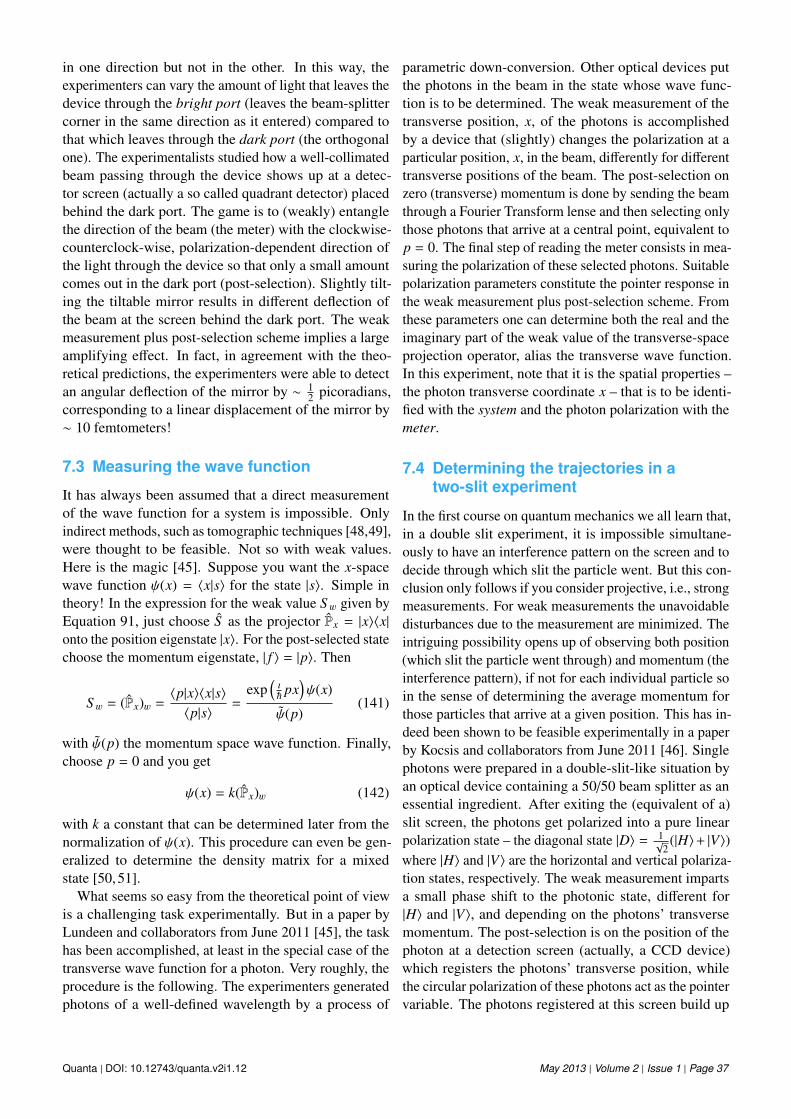
in one direction but not in the other. In this way, theexperimenters can vary the amount of light that leaves thedevice through the bright port (leaves the beam-splittercorner in the same direction as it entered) compared tothat which leaves through the dark port (the orthogonalone). The experimentalists studied how a well-collimatedbeam passing through the device shows up at a detec-tor screen (actually a so called quadrant detector) placedbehind the dark port. The game is to (weakly) entanglethe direction of the beam (the meter) with the clockwise-counterclock-wise, polarization-dependent direction ofthe light through the device so that only a small amountcomes out in the dark port (post-selection). Slightly tilt-ing the tiltable mirror results in different deflection ofthe beam at the screen behind the dark port. The weakmeasurement plus post-selection scheme implies a largeamplifying effect. In fact, in agreement with the theo-retical predictions, the experimenters were able to detectan angular deflection of the mirror by ∼ 1

2 picoradians,corresponding to a linear displacement of the mirror by∼ 10 femtometers!

7.3 Measuring the wave function

It has always been assumed that a direct measurementof the wave function for a system is impossible. Onlyindirect methods, such as tomographic techniques [48,49],were thought to be feasible. Not so with weak values.Here is the magic [45]. Suppose you want the x-spacewave function ψ(x) = 〈x|s〉 for the state |s〉. Simple intheory! In the expression for the weak value S w given byEquation 91, just choose S as the projector Px = |x〉〈x|onto the position eigenstate |x〉. For the post-selected statechoose the momentum eigenstate, | f 〉 = |p〉. Then

S w = (Px)w =〈p|x〉〈x|s〉〈p|s〉

=exp

(ı~ px

)ψ(x)

ψ(p)(141)

with ψ(p) the momentum space wave function. Finally,choose p = 0 and you get

ψ(x) = k(Px)w (142)

with k a constant that can be determined later from thenormalization of ψ(x). This procedure can even be gen-eralized to determine the density matrix for a mixedstate [50, 51].

What seems so easy from the theoretical point of viewis a challenging task experimentally. But in a paper byLundeen and collaborators from June 2011 [45], the taskhas been accomplished, at least in the special case of thetransverse wave function for a photon. Very roughly, theprocedure is the following. The experimenters generatedphotons of a well-defined wavelength by a process of

parametric down-conversion. Other optical devices putthe photons in the beam in the state whose wave func-tion is to be determined. The weak measurement of thetransverse position, x, of the photons is accomplishedby a device that (slightly) changes the polarization at aparticular position, x, in the beam, differently for differenttransverse positions of the beam. The post-selection onzero (transverse) momentum is done by sending the beamthrough a Fourier Transform lense and then selecting onlythose photons that arrive at a central point, equivalent top = 0. The final step of reading the meter consists in mea-suring the polarization of these selected photons. Suitablepolarization parameters constitute the pointer response inthe weak measurement plus post-selection scheme. Fromthese parameters one can determine both the real and theimaginary part of the weak value of the transverse-spaceprojection operator, alias the transverse wave function.In this experiment, note that it is the spatial properties –the photon transverse coordinate x – that is to be identi-fied with the system and the photon polarization with themeter.

7.4 Determining the trajectories in atwo-slit experiment

In the first course on quantum mechanics we all learn that,in a double slit experiment, it is impossible simultane-ously to have an interference pattern on the screen and todecide through which slit the particle went. But this con-clusion only follows if you consider projective, i.e., strongmeasurements. For weak measurements the unavoidabledisturbances due to the measurement are minimized. Theintriguing possibility opens up of observing both position(which slit the particle went through) and momentum (theinterference pattern), if not for each individual particle soin the sense of determining the average momentum forthose particles that arrive at a given position. This has in-deed been shown to be feasible experimentally in a paperby Kocsis and collaborators from June 2011 [46]. Singlephotons were prepared in a double-slit-like situation byan optical device containing a 50/50 beam splitter as anessential ingredient. After exiting the (equivalent of a)slit screen, the photons get polarized into a pure linearpolarization state – the diagonal state |D〉 = 1√

2(|H〉+ |V〉)

where |H〉 and |V〉 are the horizontal and vertical polariza-tion states, respectively. The weak measurement impartsa small phase shift to the photonic state, different for|H〉 and |V〉, and depending on the photons’ transversemomentum. The post-selection is on the position of thephoton at a detection screen (actually, a CCD device)which registers the photons’ transverse position, whilethe circular polarization of these photons act as the pointervariable. The photons registered at this screen build up



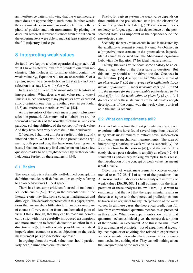
an interference pattern, showing that the weak measure-ment does not appreciably disturb them. In other words,the experimenters can simultaneously determine both thephotons’ position and their momentum. By placing thedetection screen at different distances from the slit screenthe experimenters were able to map (at least statistically)the full trajectory landscape.

8 Interpreting weak values

So far, I have kept to a rather operational approach. Allwhat I have treated follows from standard quantum me-chanics. This includes all formulae which contain theweak value S w, Equation 91, for an observable S of asystem, subject to a pre-selection in the state |s〉 and post-selection in a state | f 〉, with 〈 f |s〉 , 0.

In this section I venture to move into the territory ofinterpretation: What does a weak value really mean?This is a mined territory; many physicists have expressedstrong opinions one way or another; see, in particular,[7, 8] and references therein, as well as [52].

As the inventors of the weak measurement plus post-selection protocol, Aharonov and collaborators are theforemost advocates of the novelty, usefulness, and evenparadox-solving abilities, of the concept of weak value.And they have been very successful in their endeavor.

Of course, I shall not aim for a verdict in this slightlyinfected debate. What I will do is to present some argu-ments, both pro and con, that have some bearing on theissue. I shall not draw any final conclusion but leave a fewquestion-marks to be straightened-out by further debate.I elaborate further on these matters in [54].

8.1 Basics

The weak value is a formally well-defined concept. Itsdefinition includes well-defined entities entirely referringto an object-system’s Hilbert space.

There has been some criticism focused on mathemat-ical deficiencies [52]. True, in the presentations in theliterature one may find some cavalier mathematics andditto logic. The derivations presented in this paper, deriva-tions that are maybe a little stricter than other ones, areof course still very cavalier from a mathematical point ofview. I think, though, that they can be made mathemati-cally strict with more carefully introduced assumptionsand more attention to formal deduction; an effort in thisdirection is in [53]. In other words, possible mathematicalimperfections cannot be used as objections to the weakmeasurement plus post-selection approach..

In arguing about the weak value, one should particu-larly bear in mind three circumstances.

Firstly, for a given system the weak value depends onthree entities: the pre-selected state |s〉, the observableS , and the post-selected state | f 〉. There is sometimes atendency to forget, e.g., that the dependence on the post-selected state is as important as the dependence on thepre-selected state.

Secondly, the weak value occurs in, and is measured by,the ancilla measurement scheme. It cannot be obtained ina (projective) measurement on the system alone. In partic-ular, it cannot be derived from the Aharonov–Bergmann–Lebowitz rule Equation 17 for ideal measurements.

Thirdly, the weak value bears some analogy to an or-dinary mean value of the observable in question. Butthis analogy should not be driven too far. One sees inthe literature [55] descriptions like “the weak value ofan observable S (is) the average of a sufficiently largenumber of identical . . . weak measurements of S . . .” and“. . . the average for the sub-ensemble post-selected in thestate (| f 〉), i.e. the weak value, is given by (S w) . . .”. Ido not consider these statements to be adequate enoughdescriptions of the actual way the weak value is arrivedat in the ancilla scheme.

8.2 What can experiments tell?

As is evident even from the short presentation in section 7,experimentalists have found several ingenious ways ofusing weak measurement to extract novel informationfrom quantum mechanical measurements. The idea ofinterpreting a particular weak value as (essentially) thewave function for the system [45], and the use of deli-cately chosen post-selection to amplify an effect [42–44]stand out as particularly striking examples. In this sense,the introduction of the concept of weak value has meanta real novelty.

Other uses of weak measurements concern experi-mental tests [37, 38, 41] of some of the paradoxes thatAharonov and collaborators have analyzed in terms ofweak values [36, 39, 40]. I shall comment on the inter-pretation of these analyses below. Here, I just want toemphasize that the fact that the experimental results inthese cases agree with the theoretical prediction cannotbe taken as an argument for any interpretation of the weakvalues. In all these cases, the theoretical predictions fol-low from conventional quantum mechanics as presentedin this article. What these experiments show is thus thatquantum mechanics indeed gives the correct descriptionof their particular experiment. And this is no small feat!But as a matter of principle – not of experimental ingenu-ity, technique or of anything else related to experimentsand experimentalists – what the experiments test is quan-tum mechanics, nothing else. They can tell nothing aboutthe interpretation of the weak value.



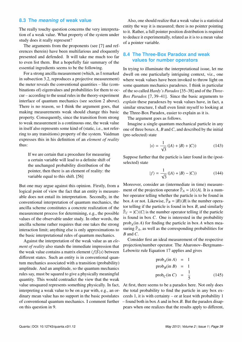
8.3 The meaning of weak value

The really touchy question concerns the very interpreta-tion of a weak value. What property of the system understudy does it really represent?

The arguments from the proponents (see [7] and ref-erences therein) have been multifarious and eloquentlypresented and defended. It will take me much too farto even list them. But a hopefully fair summary of theessential ingredients seems to be the following.

For a strong ancilla measurement (which, as I remarkedin subsection 3.2, reproduces a projective measurement)the meter reveals the conventional quantities – like (com-binations of) eigenvalues and probabilities for them to oc-cur – according to the usual rules in the theory-experimentinterface of quantum mechanics (see section 2 above).There is no reason, so I think the argument goes, thatmaking measurements weak should change this basicproperty. Consequently, since the transition from strongto weak measurement is a continuous one, the weak valuein itself also represents some kind of (static, i.e., not refer-ring to any transitions) property of the system. Vaidmanexpresses this in his definition of an element of realitythus:

If we are certain that a procedure for measuringa certain variable will lead to a definite shift ofthe unchanged probability distribution of thepointer, then there is an element of reality: thevariable equal to this shift. [56]

But one may argue against this opinion. Firstly, from alogical point of view the fact that an entity is measure-able does not entail its interpretation. Secondly, in theconventional interpretation of quantum mechanics, theancilla scheme constitutes a concrete realization of themeasurement process for determining, e.g., the possiblevalues of the observable under study. In other words, theancilla scheme rather requires that one takes the stronginteraction limit; anything else is only approximations tothe basic interpretational rules of quantum mechanics.

Against the interpretation of the weak value as an ele-ment of reality also stands the immediate impression thatthe weak value contains a matrix element 〈 f |S |s〉 betweendifferent states. Such an entity is in conventional quan-tum mechanics associated with a transition (probability)amplitude. And an amplitude, so the quantum mechanicsrules say, must be squared to give a physically meaningfulquantity. This would contradict the view that the weakvalue unsquared represents something physically. In fact,interpreting a weak value to be on a par with, e.g., an or-dinary mean value has no support in the basic postulatesof conventional quantum mechanics. I comment furtheron this question in 9.

Also, one should realize that a weak value is a statisticalentity the way it is measured; there is no pointer pointingto it. Rather, a full pointer position distribution is requiredto deduce it experimentally, related as it is to a mean valueof a pointer variable.

8.4 The Three-Box Paradox and weakvalues for number operators

In trying to illuminate the interpretational issue, let medwell on one particularly intriguing context, viz., onewhere weak values have been invoked to throw light onsome quantum mechanics paradoxes. I think in particularof the so called Hardy’s Paradox [35–38] and of the Three-Box Paradox [7, 39–41]. Since the basic arguments toexplain these paradoxes by weak values have, in fact, asimilar structure, I shall even limit myself to looking atthe Three-Box Paradox, easier to explain as it is.

The argument goes as follows.Imagine a single quantum mechanical particle in any

one of three boxes A, B and C, and described by the initial(pre-selected) state

|s〉 =1√

3(|A〉 + |B〉 + |C〉) (143)

Suppose further that the particle is later found in the (post-selected) state

| f 〉 =1√

3(|A〉 + |B〉 − |C〉) (144)

Moreover, consider an (intermediate in time) measure-ment of the projection operator PA = |A〉〈A|. It is a num-ber operator telling whether the particle is to be found inbox A or not. Likewise, PB = |B〉〈B| is the number opera-tor telling if the particle is found in box B, and similarlyPC = |C〉〈C| is the number operator telling if the particleis found in box C. One is interested in the probabilityprobA(in A) for finding the particle in box A when mea-suring PA, as well as the corresponding probabilities forB and C.

Consider first an ideal measurement of the respectiveprojection/number operator. The Aharonov–Bergmann–Lebowitz rule Equation 17 applies and gives

probA(in A) = 1

probB(in B) = 1

probC(in C) =15

(145)

At first, there seems to be a paradox here. Not only doesthe total probability to find the particle in any box ex-ceeds 1, it is with certainty – or at least with probability 1– found both in box A and in box B. But the paradox disap-pears when one realizes that the results apply to different,



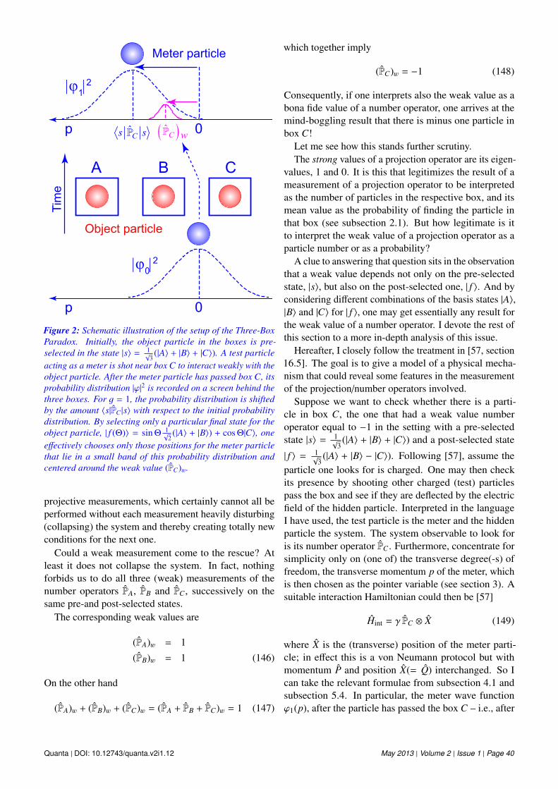
A B C

p 0

p 0

Tim

eMeter particle

Object particle

ˆCs s ( )ˆ

C w

|ϕ1|2

|ϕ0|2

Figure 2: Schematic illustration of the setup of the Three-BoxParadox. Initially, the object particle in the boxes is pre-selected in the state |s〉 = 1

√3(|A〉 + |B〉 + |C〉). A test particle

acting as a meter is shot near box C to interact weakly with theobject particle. After the meter particle has passed box C, itsprobability distribution |ϕ|2 is recorded on a screen behind thethree boxes. For g = 1, the probability distribution is shiftedby the amount 〈s|PC |s〉 with respect to the initial probabilitydistribution. By selecting only a particular final state for theobject particle, | f (Θ)〉 = sin Θ 1

√2(|A〉 + |B〉) + cos Θ|C〉, one

effectively chooses only those positions for the meter particlethat lie in a small band of this probability distribution andcentered around the weak value (PC)w.

projective measurements, which certainly cannot all beperformed without each measurement heavily disturbing(collapsing) the system and thereby creating totally newconditions for the next one.

Could a weak measurement come to the rescue? Atleast it does not collapse the system. In fact, nothingforbids us to do all three (weak) measurements of thenumber operators PA, PB and PC , successively on thesame pre-and post-selected states.

The corresponding weak values are

(PA)w = 1

(PB)w = 1 (146)

On the other hand

(PA)w + (PB)w + (PC)w = (PA + PB + PC)w = 1 (147)

which together imply

(PC)w = −1 (148)

Consequently, if one interprets also the weak value as abona fide value of a number operator, one arrives at themind-boggling result that there is minus one particle inbox C!

Let me see how this stands further scrutiny.The strong values of a projection operator are its eigen-

values, 1 and 0. It is this that legitimizes the result of ameasurement of a projection operator to be interpretedas the number of particles in the respective box, and itsmean value as the probability of finding the particle inthat box (see subsection 2.1). But how legitimate is itto interpret the weak value of a projection operator as aparticle number or as a probability?

A clue to answering that question sits in the observationthat a weak value depends not only on the pre-selectedstate, |s〉, but also on the post-selected one, | f 〉. And byconsidering different combinations of the basis states |A〉,|B〉 and |C〉 for | f 〉, one may get essentially any result forthe weak value of a number operator. I devote the rest ofthis section to a more in-depth analysis of this issue.

Hereafter, I closely follow the treatment in [57, section16.5]. The goal is to give a model of a physical mecha-nism that could reveal some features in the measurementof the projection/number operators involved.

Suppose we want to check whether there is a parti-cle in box C, the one that had a weak value numberoperator equal to −1 in the setting with a pre-selectedstate |s〉 = 1√

3(|A〉 + |B〉 + |C〉) and a post-selected state

| f 〉 = 1√3(|A〉 + |B〉 − |C〉). Following [57], assume the

particle one looks for is charged. One may then checkits presence by shooting other charged (test) particlespass the box and see if they are deflected by the electricfield of the hidden particle. Interpreted in the languageI have used, the test particle is the meter and the hiddenparticle the system. The system observable to look foris its number operator PC . Furthermore, concentrate forsimplicity only on (one of) the transverse degree(-s) offreedom, the transverse momentum p of the meter, whichis then chosen as the pointer variable (see section 3). Asuitable interaction Hamiltonian could then be [57]

Hint = γ PC ⊗ X (149)

where X is the (transverse) position of the meter parti-cle; in effect this is a von Neumann protocol but withmomentum P and position X(= Q) interchanged. So Ican take the relevant formulae from subsection 4.1 andsubsection 5.4. In particular, the meter wave functionϕ1(p), after the particle has passed the box C – i.e., after



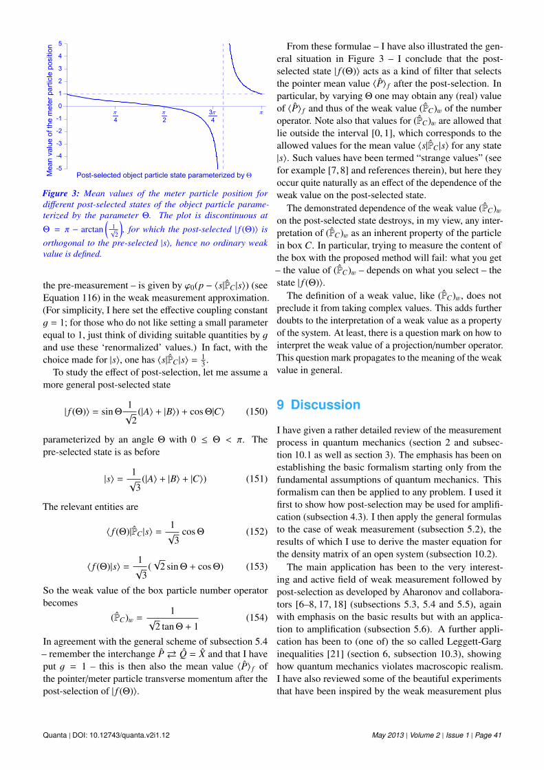
5

4

3

2

1

0

-1

-2

-3

-4

-5

4π

2π 3

4π π

Post-selected object particle state parameterized by ΘMea

n va

lue

of th

e m

eter

par

ticle

pos

ition

Figure 3: Mean values of the meter particle position fordifferent post-selected states of the object particle parame-terized by the parameter Θ. The plot is discontinuous at

Θ = π − arctan(

1√

2

), for which the post-selected | f (Θ)〉 is

orthogonal to the pre-selected |s〉, hence no ordinary weakvalue is defined.

the pre-measurement – is given by ϕ0(p − 〈s|PC |s〉) (seeEquation 116) in the weak measurement approximation.(For simplicity, I here set the effective coupling constantg = 1; for those who do not like setting a small parameterequal to 1, just think of dividing suitable quantities by gand use these ‘renormalized’ values.) In fact, with thechoice made for |s〉, one has 〈s|PC |s〉 = 1

3 .To study the effect of post-selection, let me assume a

more general post-selected state

| f (Θ)〉 = sin Θ1√

2(|A〉 + |B〉) + cos Θ|C〉 (150)

parameterized by an angle Θ with 0 ≤ Θ < π. Thepre-selected state is as before

|s〉 =1√

3(|A〉 + |B〉 + |C〉) (151)

The relevant entities are

〈 f (Θ)|PC |s〉 =1√

3cos Θ (152)

〈 f (Θ)|s〉 =1√

3(√

2 sin Θ + cos Θ) (153)

So the weak value of the box particle number operatorbecomes

(PC)w =1

√2 tan Θ + 1

(154)

In agreement with the general scheme of subsection 5.4– remember the interchange P Q = X and that I haveput g = 1 – this is then also the mean value 〈P〉 f ofthe pointer/meter particle transverse momentum after thepost-selection of | f (Θ)〉.

From these formulae – I have also illustrated the gen-eral situation in Figure 3 – I conclude that the post-selected state | f (Θ)〉 acts as a kind of filter that selectsthe pointer mean value 〈P〉 f after the post-selection. Inparticular, by varying Θ one may obtain any (real) valueof 〈P〉 f and thus of the weak value (PC)w of the numberoperator. Note also that values for (PC)w are allowed thatlie outside the interval [0, 1], which corresponds to theallowed values for the mean value 〈s|PC |s〉 for any state|s〉. Such values have been termed “strange values” (seefor example [7,8] and references therein), but here theyoccur quite naturally as an effect of the dependence of theweak value on the post-selected state.

The demonstrated dependence of the weak value (PC)won the post-selected state destroys, in my view, any inter-pretation of (PC)w as an inherent property of the particlein box C. In particular, trying to measure the content ofthe box with the proposed method will fail: what you get– the value of (PC)w – depends on what you select – thestate | f (Θ)〉.

The definition of a weak value, like (PC)w, does notpreclude it from taking complex values. This adds furtherdoubts to the interpretation of a weak value as a propertyof the system. At least, there is a question mark on how tointerpret the weak value of a projection/number operator.This question mark propagates to the meaning of the weakvalue in general.

9 Discussion

I have given a rather detailed review of the measurementprocess in quantum mechanics (section 2 and subsec-tion 10.1 as well as section 3). The emphasis has been onestablishing the basic formalism starting only from thefundamental assumptions of quantum mechanics. Thisformalism can then be applied to any problem. I used itfirst to show how post-selection may be used for amplifi-cation (subsection 4.3). I then apply the general formulasto the case of weak measurement (subsection 5.2), theresults of which I use to derive the master equation forthe density matrix of an open system (subsection 10.2).

The main application has been to the very interest-ing and active field of weak measurement followed bypost-selection as developed by Aharonov and collabora-tors [6–8, 17, 18] (subsections 5.3, 5.4 and 5.5), againwith emphasis on the basic results but with an applica-tion to amplification (subsection 5.6). A further appli-cation has been to (one of) the so called Leggett-Garginequalities [21] (section 6, subsection 10.3), showinghow quantum mechanics violates macroscopic realism.I have also reviewed some of the beautiful experimentsthat have been inspired by the weak measurement plus



post-selection approach [25,28,32–34,37,38,41–47] (sec-tion 7), experiments that show amplification in action orrelax some of the restrictions that are attached to thestandard, projective (strong) quantum mechanical mea-surement scheme.

With respect to the weak measurement plus post-selection approach, I have thus shown that it requiresno new features besides conventional quantum mechanicsto arrive at the main results. I have specially stressed theessential role played by the post-selection component ofthe scheme. This is particularly true in the applicationsof the approach to some of the so called paradoxes ofquantum mechanics( [35, 36, 39, 40]). The crucial issuehere is the meaning of the weak value of a number orprojection operator: is it legitimate to interprete a weakvalue like (PC)w of Equation 148 literally as a number?

Some arguments that have been put forward to supportsuch an interpretation can be disposed of. The fact thatexperiments agree with the calculated value has no bear-ing on the interpretation (subsection 8.2). Nor has thefact that the weak value is a measureable quantity: themere fact that a quantity is measureable does not entailsits interpretation.

With the Three-Box Paradox as an example, I havealso shown concretely (subsection 8.4) that a literal in-terpretation of the weak value of a number operator isdifficult to uphold: invoking the crucial dependence ofthe weak value on the post-selected state, essentially any(complex) value of the weak value (PC)wmay be obtained(see also [54]).

Indeed, on a very fundamental level, it is difficult tosee how a literal interpretation of a weak value can bededuced from the basic postulates of quantum mechanics.In other words, it seems to me that Aharonov and collabo-rators go beyond conventional quantum mechanics whenthey do this: in some way or other, they have extendedthe usual list of quantum mechanical postulates. I refrainfrom an opinion on whether the outcome of this extensionis profitable. What I have shown is, anyhow, that it resultsin complex values for what they interpret as a number, afact that I find awkward.

Acknowledgement

I thank Stefan Kroll, Lloyd Sanders and Bo Soderbergfor comments on (part of) the manuscript, Mats-Erik Pis-tol for constructive suggestions, Holger F. Hoffman forinteresting discussions over the net and for drawing myattention to the work [18], Sahel Ashhab for a carefulreading of the first version of this article, and DankoGeorgiev for very constructive editing of my manuscript.

10 Appendix

10.1 Some properties of measurementoperators and effects, alias POVM

The so called measurement operators are defined in termsof the pre-measurement unitary evolution operator U insubsection 3.3. They play a relatively minor role in mypresentation. This is because I prefer to rely on moreexplicit expressions for U, and to derive the results I wantfrom the ensuing time-evolution of the density matrices.However, in more general treatments of the measurementprocess in quantum mechanics, they and the effects – tobe defined in point (7) below – play a much more centralrole; see [5, section 1.4.1]. Therefore, it is of interest alsohere to list and derive some of their properties, which Ido in this appendix, making heavy use of the notation andthe results from section 3.

10.1.1 Basic properties

1. A measurement operator is defined by

Ωk = 〈mk|U |m(0)〉 (155)

It is an operator in the Hilbert spaceHS of the sys-tem.

2. Some elementary relations are

Ωk = 〈mk|U |m(0)〉

=∑

i

〈mk|m(i)〉|si〉〈si|

=∑

i

〈mk|m(i)〉Psi (156)

3. If one compares the expression

σ1(|mk) =Ωkσ0Ω

†

k

prob (mk)(157)

to the Luders’ rule

σ1(|si) =Psiσ0Psi

prob(si|σ0)(158)

in a projective measurement, one sees that the mea-surement operators Ωk play the role of a kind ofgeneralized projectors. However, they do obey dif-ferent rules from ordinary projectors.

4. Projectors obey

P†si= Psi (159)

Psi Ps j = δi, jPsi (160)



For measurement operators such rules, in general,are not valid

Ω†

k =∑

i

〈m(i)|mk〉Psi , Ωk (161)

and

Ω†

kΩl = (∑

i

〈m(i)|mk〉Psi)† × (

∑j

〈ml|m( j)〉Ps j)

=∑

i

〈m(i)|mk〉Psi〈ml|m(i)〉 (162)

which in general has no simple relation to either Ωk

or Ωl; remember that the states |m(i)〉 in general donot form a complete set inHM.

5. Note however that

Ω†

kΩk =∑

i

〈m(i)|mk〉Psi〈mk|m(i)〉

=∑

i

|〈m(i)|mk〉|2Psi (163)

implying that ∑k

Ω†

kΩk = IS (164)

with IS the unit operator in the system Hilbert spaceHS; in deriving this relation I have used the factsthat the basis states |mk〉 in the meter Hilbert spaceHM form a complete set, and that the states |m(i)〉

are normalized. This relation could be compared tothe completeness relation∑

i

Psi = IS (165)

for usual projectors.

6. The measurement operators also enter into the ex-pression for the probability prob(mk) to obtain thevalue mk:

TrS(Ωkσ0Ω

†

k

)= TrS

(Ω†

kΩkσ0)

=∑

j

∑i

∣∣∣∣∣〈m(i)|mk〉

∣∣∣∣∣2〈s j|Psiσ0|s j〉

=

∑i

∣∣∣∣∣〈m(i)|mk〉

∣∣∣∣∣2〈si|σ0|si〉

= prob(mk) (166)

In fact, this is a consistency condition, since it isequivalent to the normalization condition

TrS σ1(|mk) = 1 (167)

7. The product Ω†

kΩk = Ek, appearing naturally inthis expression for prob(mk), has many names. Itis called effect or probability operator, sometimesalternatively positive-operator valued measure (ab-breviated POVM). With this notation, the relationgiven by Equation 164 reads∑

k

Ek = IS (168)

It is an expression of the fact that probabilities

prob(mk) = TrS(Ekσ0

)(169)

sum to unity. Thus not only the measurement opera-tors Ωk but also the effects Ek have properties similarto projectors. The effects are Hermitian

E†

k = Ek (170)

but in general not idempotent

EkEl , δk,lEk (171)

8. A more realistic model of the ancilla scheme takesinto account the fact that the measurement processcould involve more degrees of freedom than thepointer observable M and the one, S , to be mea-sured for the system. So let me suppose that theadded degrees of freedom, referred to as D, aredescribed in a Hilbert space HD with basis states|dr〉, r = 1, 2, . . . , dD = dim(HD). The initial stateis |d(0)〉. The pre-measurement prescription Equa-tion 25 of subsection 3.2 is replaced by:

|si〉 ⊗ |d(0)〉 ⊗ |m(0)〉U−→ U(|si〉 ⊗ |d(0)〉 ⊗ |m(0)〉)

= |si〉 ⊗ |d(i)〉 ⊗ |m(i)〉 (172)

Thus, the measurement process is supposed to influ-ence also the new degrees of freedom. The differ-ence is that they are of no interest for that processand must consequently be summed over. In partic-ular, when forming the conditional density matrixσ1(|mk) after the read out of M with the result mk,one must trace out also the D degrees of freedom(see subsection 3.3), resulting in

σ1(|mk) = TrM,D (τ1(|mk))

=TrM,D

[(IS ⊗ ID ⊗ Omk

)τ1

(IS ⊗ ID ⊗ Omk

)]prob(mk)

=

∑r

(〈dr |〈mk|U |d(0)〉|m(0)〉σ0〈m(0)|〈d(0)|U†|mk〉|dr〉

)prob(mk)

=1

prob(mk)

∑r

Ωk,rσ0Ω†

k,r (173)



with

Ωk,r = 〈dr |〈mk|U |d(0)〉|m(0)〉

=∑

i

〈mk|m(i)〉〈dr |d(i)〉Psi (174)

The probability becomes

prob(mk) = TrS(∑

r

Ωk,rσ0Ω†

k,r)

=∑

r

TrS(Ω†k,rΩk,rσ0) (175)

implying that the effects read

Ek =∑

r

Ω†

k,rΩk,r (176)

The expressions for the relations between the densitymatrix σ1(|mk), the measurement operators Ωk,r, andthe effects Ek derived here are the most general onesin the general theory of measurement (see [5, section1.4.1]).

10.1.2 Realization in the von Neumann protocol

The von Neumann protocol of subsection 4.1 lives in theq-basis. This means the following concrete realizationsof the measurement operators

Ωk =∑

i

〈mk|m(i)〉Psi

→ Ωq =∑

i

ϕi(q)Psi

=∑

i

ϕ0(q − gsi)Psi (177)

For the effects

Ek =∑

i

|〈m(i)|mk〉|2Psi

→ Eq =∑

i

|ϕ0(q − gsi)|2Psi (178)

10.1.3 Realization in the double qubit protocol

In the double qubit protocol of subsection 4.2, there aretwo measurement operators, Ω0 and Ω1. They take theform (recall what I said in subsection 4.2 concerning theswitch to a computational basis notation!)

Ω0 = 〈0|M|m(si=+1)〉MPsi=+1 + 〈0|M|m(si=−1)〉MPsi=−1

= cosϑ

2|0〉S〈0|S + sin

ϑ

2|1〉S〈1|S

=

(cos ϑ

2 00 sin ϑ

2

)(179)

Ω1 = 〈1|M|m(si=+1)〉MPsi=+1 + 〈1|M|m(si=−1)〉MPsi=−1

= sinϑ

2|0〉S〈0|S + cos

ϑ

2|1〉S〈1|S

=

(sin ϑ

2 00 cos ϑ

2

)(180)

where I explicitly introduced the matrix representations.The effects then become

E0 = Ω†

0Ω0 =

(cos2 ϑ

2 00 sin2 ϑ

2

)(181)

E1 = Ω†

1Ω1 =

(sin2 ϑ

2 00 cos2 ϑ

2

)(182)

10.2 Continuous measurements, thequantum Zeno effect, and the masterequation for an open system

The treatment of weak measurement in the ancilla schemein subsection 5.2 is a convenient starting point for treatingcontinuous measurements and for handling the influenceof interaction with an environment for an open system.The transition to a continuous measurement is accom-plished by performing a limit in which the time durationδtU of the pre-measurement interaction between the sys-tem and the meter tends to zero. It is not straight-forward,though, just to take the limit δtU → 0; some efforts arerequired in order to overcome a few stumbling blocks. Inthis appendix I give a broad outline of how this can bedone.

10.2.1 The quantum Zeno effect

I will consider a continuous measurement as the limitof a sequence of consecutive measurements, carried outat regular time intervals of a duration δtU , which tendto zero. Thus, I model it by assuming the system to besubjected to n consecutive, identical measurements intime intervals between fixed times t = t0 and t = t f = tn.The difference tr−tr−1 between any two consecutive timesis assumed to tend to zero as n → ∞. Indeed, I assumeeach pre-measurement U = exp(− ı

~γ S ⊗ P δtU) to be ofduration δtU and to occur in the time interval betweenthe indicated times so that tr − tr−1 = δtU , r = 1, 2, . . . , n.The limit to be taken is then δtU → 0, n → ∞ but suchthat n × δtU = t f − t0 remains finite and non-vanishing.Consequently, a weak interaction approximation for Uapplies.

It follows from Equation 39 of subsection 3.4 that thesystem density matrix σn, after n such identical, consecu-tive measurements, reads

σn =∑i, j

Psiσ0Ps j

(〈m( j)|m(i)〉

)n(183)



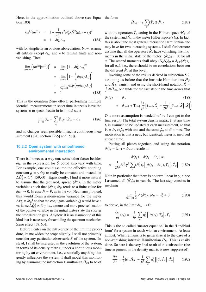
Here, in the approximation outlined above (see Equa-tion 100)

〈m( j)|m(i)〉 ≈ 1 −1

2~2γ2δt2

U〈N2〉0(si − s j)2

= 1 − δt2U Ai j (184)

with for simplicity an obvious abbreviation. Now, assumeall entities except δtU and n to remain finite and non-vanishing. Then

limn→∞

(〈m( j)|m(i)〉

)n= lim

n→∞

(1 − δt2

U Ai j)n

= limn→∞

(1 −

1nδtU t f Ai j

)n

= limδtU→0

exp(−δtU t f Ai j

)= 1 (185)

This is the quantum Zeno effect: performing multipleidentical measurements in short time intervals leave thesystem so to speak frozen in its initial state

limn→∞

σn =∑i, j

Psiσ0Ps j = σ0 (186)

and no changes seem possible in such a continuous mea-surement ( [20, section 12-5] and [58]).

10.2.2 Open system with smoothenedenvironmental interaction

There is, however, a way out: some other factor besidesδtU in the expression for U could also vary with time.For example, one could assume the effective couplingconstant g = γ δtU to really be constant and instead let∆Q2

0 ∝ δt−1U [59, 60]. Equivalently, I find it more natural

to assume that the (squared) spread 〈N2〉0 in the metervariable is such that 〈N2〉0 δtU tends to a finite value forδtU → 0. In case N = P, as in the von Neumann protocol,this would mean a momentum variance for the meter∆P2

0 ∝ δt−1U so that the conjugate variable Q would have a

variance ∆Q20 ∝ δtU i.e., a more and more precise location

of the pointer variable in the initial meter state the shorterthe time duration gets. Anyhow, it is an assumption of thiskind that is necessary for avoiding the quantum mechanicsZeno effect [59, 60].

Before I enter on the nitty-gritty of the limiting proce-dure, let me widen the scope slightly. I shall not primarilyconsider any particular observable S of the system. In-stead, I shall be interested in the evolution of the system,in terms of its density matrix, under a continuous moni-toring by an environment, i.e., essentially anything thatgently influences the system. I shall model this monitor-ing by assuming the interaction Hamiltonian Hint to be of

the formHint = γ

∑a

(Ta ⊗ Na) (187)

with the operators Ta acting in the Hilbert space HS ofthe system and Na in the meter Hilbert spaceHM. In fact,this is about the most general interaction Hamiltonian onemay have for two interacting systems. I shall furthermoreassume that all the operators Na have vanishing first mo-ments in the initial state of the meter: 〈Na〉0 = 0, for alla. The second moments shall obey 〈NaNb〉0 = δa,b〈N2

a〉0,for all a, b, i.e., there should be no correlations betweenthe different Na at this level.

Invoking some of the results derived in subsection 5.2,assuming as before that the intrinsic Hamiltonians HSand HM vanish, and using the short-hand notation X =∫

dtHint, one finds for the last step in the time-series that

σ(t f ) = σn (188)

≈ σn−1 + TrM

(ı

~

[τn−1, X

]−

12~2

[[τn−1, X

], X

])One more assumption is needed before I can get to thefinal result: The total system density matrix τr at any timetr is assumed to be updated at each measurement, so thatτr = σr ⊗ µ0 with one and the same µ0 at all times. Themotivation is that a new, but identical, meter is involvedat each time.

Putting all pieces together, and using the notationσ(t f − δtU) = σn−1, results in

σ(t f ) − σ(t f − δtU) ≈

≈ −1

2~2 δt2Uγ

2∑

a

〈N2a〉0

[[σ(t f − δtU), Ta

], Ta

](189)

Note in particular that there is no term linear in γ, sinceI assumed all 〈Na〉0 to vanish. The last step consists ininvoking

limδtU→0

12γ2〈N2

a〉0 δtU = η2a , 0 (190)

to derive, in the limit δtU → 0:

∂σ

∂t(t f ) = −

1~2

∑a

η2a

[[σ(t f ), Ta

], Ta

](191)

This is the so called ‘master equation’ in the ‘Lindbladform’ for a system in touch with an environment. At leastalmost. What remains is to generalize it to the case of anon-vanishing intrinsic Hamiltonian HS. This is easilydone. So here is the very final result of this subsection (thetime argument in the density matrix is now suppressed)

∂σ

∂t=ı

~[σ, HS] −

1~2

∑a

η2a

[[σ, Ta

], Ta

](192)



One may question some of the assumptions made inderiving this master equation. Indeed, other less pedes-trian methods must be applied in a stricter derivation. Thepoor man’s derivation presented here may anyhow be mo-tivated by its comparative simplicity. See, e.g., [5, chapter3], and [61, 62] for more basic approaches. I shall notdwell upon applications of the master equation but referto the literature. Let me only mention that one impor-tant such application is the study of decoherence due tointeraction with the environment [5, chapter 3], and [62].

10.3 The Leggett–Garg inequality

From a few reasonable assumptions on what character-izes the macro world, Leggett and Garg [21] were able todeduce inequalities involving (in general different) mea-surements performed at successive times but on one andthe same object-system. These inequalities are then gen-eralized to the micro domain. In this appendix, I sketchthe derivation of (one of) these inequalities, the one usedin section 6.

The assumptions invoked by Leggett and Garg are,slightly reformulated

• Macroscopic realism: A macroscopic system will atall times be in one or the other of the states availableto it.

• Noninvasive detection: It is possible to determine thestate of the system with arbitrary small perturbationson its subsequent dynamics.

The set-up for Leggett–Garg inequality consists of threesuccessive measurements of the observables A0, A1 andA2. For purely simplifying purposes, I shall assume thatthere is no time evolution in between the appropriatemeasurements.

Consider first how the argument based on macroscopicreasoning goes. Suppose the result of a measurement ofthe observable Ai is ai, i = 0, 1, 2. Suppose also that allthe ai lie in the interval [−1,+1]. Leggett and Garg thenconsider the combination

B = a0a1 + a1a2 − a2a0 (193)

It is straight-forward to show the inequality

− 3 ≤ B ≤ 1 (194)

Averaging B over the probability distributions for obtain-ing the respective values does not destroy the inequality– there are some subtleties involved, and one must ofcourse use the fact that probabilities lie between 0 and +1as well as the assumptions of macroscopic realism andnoninvasive detection in the derivation – so with

〈B〉 = 〈A0A1〉 + 〈A1A2〉 − 〈A2A0〉 (195)

(bra-kets 〈. . .〉 denote averages over the respective proba-bility distributions), one arrives at

− 3 ≤ 〈B〉 ≤ 1 (196)

This inequality is then taken over to the micro domainby interpreting classical averages, like 〈A0A1〉 , as quan-tum mechanical expectation values 〈A0A1〉 etc. of thecorresponding operators in an initial state prepared be-fore the measurement of A0 takes place. It constitutesone of the Leggett–Garg inequalities; other inequalitiesmay be obtained by invoking more than three consecutivemeasurements.

The Leggett–Garg framework is aptly suited for studiesusing weak measurement: For a weak measurement, thecondition of noninvasive measurement can be considered(approximately) fulfilled. Therefore, with weak measure-ment, the Leggett–Garg inequality effectively only teststhe macrorealism assumption. One may even relax a biton the requirement of weak measurements. In fact, themain steps in the derivation of the Leggett–Garg inequal-ity really only require the middle measurement, that of A1,to be weak. Both initially and finally, for A0 respectivelyA2, the measurement could be projective.

The actual applications [28, 32–34] even choose A0 =

|s〉〈s|, the projection operator on the initial (‘pre-selected’)state. The Leggett–Garg entity 〈B〉 then reads

〈B〉 = 〈s|A1|s〉 + 〈s|A1A2|s〉 − 〈s|A2|s〉 (197)

where, as remarked, A2 may be measured projectivelyand only A1 is required to be measured weakly. In theexperimental realizations, different choices for A1 and A2have been investigated [32–34].

One could fit the Leggett–Garg inequality even moreclosely to the theme of this article by considering a weakmeasurement plus post-selection situation. By this I meanmaking the substitutions

A0 → σ0 = |s〉〈s| (198)

A1 → S (199)

A2 → | f 〉〈 f | (200)

which for 〈 f |s〉 , 0 result in

〈B〉 = 〈s|S |s〉 + 〈s|S | f 〉〈 f |s〉 − 〈s| f 〉〈 f |s〉

= 〈s|S |s〉 + |〈 f |s〉|2(S w − 1) (201)

This expression involves the weak value S w, given byEquation 91, of the observable S .

Note, however, that there is an inherent order ambiguityin translating a classical mean value of a product of twoobservables into a quantum mechanical expectation valuewhen the two corresponding operators do not commute.



In the last example, this is reflected in the fact that S w, acomplex number in general, appears in 〈B〉. I propose tosolve the ambiguity by replacing an operator product, sayA1A2, by the symmetrized one, 1

2 (A1A2 + A2A1).Then, provided all the eigenvalues si of S lie in the

interval [−1,+1], the final expression for the Leggett–Garg inequality becomes in this case

−3 ≤ 〈B〉 ≤ 1 (202)

〈B〉 = 〈s|S |s〉 + |〈 f |s〉|2 [Re(S w) − 1] (203)

I devote section 6 of the main text to an analysis of thisparticular version of Leggett–Garg inequality in the dou-ble qubit setup.

Summing up, the weak ancilla protocol has the advan-tage in connection with Leggett–Garg inequality that itobeys the non-invasive detection assumption, in the limitof a very weak pre-measurement interaction, g → 0. Inparticular, any violation of the Leggett–Garg inequalitycan then be blamed on the violation of the macroscopicrealism assumption.

References

[1] von Neumann J. Matematische Grundlagen derQuantenmechanik. Springer Verlag, 1932. [Englishtranslation: Mathematical Foundations of QuantumMechanics. Princeton University Press, 1955]

[2] Wheeler JA, Zurek WH. Quantum theory and mea-surement. Princeton University Press, 1983.

[3] Braginsky VB, Khalili FY. Quantum Measurement.Cambridge: Cambridge University Press, 1992.

[4] Nielsen MA, Chuang IL. Quantum Computationand Quantum Information, 10th Anniversary edition.Cambridge: Cambridge University Press, 2011.

[5] Wiseman HM, Milburn GJ. Quantum Measurementand Control. Cambridge: Cambridge UniversityPress, 2009.

[6] Aharonov Y, Albert DZ, Vaidman L. How the resultof a measurement of a component of the spin of aspin-1/2 particle can turn out to be 100. PhysicalReview Letters 1988; 60 (14): 1351-1354. http://dx.doi.org/10.1103/PhysRevLett.60.1351

[7] Aharonov Y, Vaidman L. The two-state vectorformalism: an updated review. In: Time inQuantum Mechanics, vol.734, Muga JG, MayatoRS, Egusquiza IL (editors), Springer Berlin Hei-delberg, 2007, pp.399-447. http://arxiv.org/abs/quant-ph/0105101

[8] Aharonov Y, Popescu S, Tollaksen J. A time-symmetric formulation of quantum mechanics.Physics Today 2010; 63 (11): 27-32. http://dx.doi.org/10.1063/1.3518209

[9] Nauenberg M. Time-symmetric quantum mechan-ics questioned and defended. Physics Today 2011;64 (5): 8. http://dx.doi.org/10.1063/1.3592020

[10] Hobson A. Time-symmetric quantum mechanicsquestioned and defended. Physics Today 2011;64 (5): 8-9. http://dx.doi.org/10.1063/1.3595152

[11] Mukamel S. Time-symmetric quantum mechan-ics questioned and defended. Physics Today 2011;64 (5): 9,62. http://dx.doi.org/10.1063/1.3595153

[12] Griffiths RB. Time-symmetric quantum mechan-ics questioned and defended. Physics Today 2011;64 (5): 62. http://dx.doi.org/10.1063/1.3595149

[13] Aharonov Y, Popescu S, Tollaksen J. Time-symmetric quantum mechanics questioned and de-fended. Physics Today 2011; 64 (5): 62-63. http://dx.doi.org/10.1063/1.3595150

[14] Mermin ND. Consistent treatments of quantum me-chanics. Physics Today 2011; 64 (10): 8-9. http://dx.doi.org/10.1063/PT.3.1271

[15] Griffiths RB. Consistent treatments of quantum me-chanics. Physics Today 2011; 64 (10): 9. http://dx.doi.org/10.1063/PT.3.1272

[16] Aharonov Y, Popescu S, Tollaksen J. Consistenttreatments of quantum mechanics. Physics Today2011; 64 (10): 9-10. http://dx.doi.org/10.1063/PT.3.1273

[17] Cho A. Furtive approach rolls back the limitsof quantum uncertainty. Science 2011; 333(6043): 690-693. http://dx.doi.org/10.

1126/science.333.6043.690

[18] Kofman AG, Ashhab S, Nori F. Nonperturbativetheory of weak pre- and post-selected measurements.Physics Reports 2012; 520 (2): 43-133. http://dx.doi.org/10.1016/j.physrep.2012.07.001

[19] Griffiths DJ. Introduction to Quantum Mechanics.Pearson Prentice Hall, 2004.


http://dx.doi.org/10.1103/PhysRevLett.60.1351


http://arxiv.org/abs/quant-ph/0105101


http://dx.doi.org/10.1063/1.3518209

http://dx.doi.org/10.1063/1.3518209

http://dx.doi.org/10.1063/1.3592020

http://dx.doi.org/10.1063/1.3592020

http://dx.doi.org/10.1063/1.3595152

http://dx.doi.org/10.1063/1.3595152

http://dx.doi.org/10.1063/1.3595153

http://dx.doi.org/10.1063/1.3595153

http://dx.doi.org/10.1063/1.3595149

http://dx.doi.org/10.1063/1.3595149

http://dx.doi.org/10.1063/1.3595150

http://dx.doi.org/10.1063/1.3595150

http://dx.doi.org/10.1063/PT.3.1271






http://dx.doi.org/10.1126/science.333.6043.690

http://dx.doi.org/10.1126/science.333.6043.690

http://dx.doi.org/10.1016/j.physrep.2012.07.001

http://dx.doi.org/10.1016/j.physrep.2012.07.001


[20] Peres A. Quantum Theory: Concepts and Methods.Kluwer, 1993.

[21] Leggett AJ, Garg A. Quantum mechanics ver-sus macroscopic realism: Is the flux there whennobody looks? Physical Review Letters 1985;54 (9): 857-860. http://dx.doi.org/10.1103/PhysRevLett.54.857

[22] Luders G. Uber die Zustandanderung durchden Meßprozeß. Annalen der Physik (Leipzig)1951; 443 (8): 322-328. http://dx.doi.org/10.1002/andp.19504430510

[23] Aharonov Y, Bergmann PG, Lebowitz JL. Timesymmetry in the quantum process of measurement.Physical Review B 1964; 134 (6): 1410-1416. http://dx.doi.org/10.1103/PhysRev.134.B1410

[24] Di Lorenzo A, Egues JC. Weak measurement: Effectof the detector dynamics. Physical Review A 2008;77 (4): 042108. http://dx.doi.org/10.1103/PhysRevA.77.042108

[25] Pryde GJ, O’Brien JL, White AG, Ralph TC, Wise-man HM. Measurement of quantum weak values ofphoton polarization. Physical Review Letters 2005;94 (22): 220405. http://dx.doi.org/10.1103/PhysRevLett.94.220405

[26] Wu S, Mølmer K. Weak measurements with a qubitmeter. Physics Letters A 2009; 374 (1): 34-39.http://arxiv.org/abs/0909.0841

[27] Brun TA, Diosi L, Strunz WT. Test of weak measure-ment on a two- or three-qubit computer. PhysicalReview A 2008; 77 (3): 032101. http://arxiv.org/abs/0711.4149

[28] Langford NK, Weinhold TJ, Prevedel R, ReschKJ, Gilchrist A, O’Brien JL, Pryde GJ, WhiteAG. Demonstration of a simple entangling opti-cal gate and its use in Bell-state analysis. Physi-cal Review Letters 2005; 95 (21): 210504. http://arxiv.org/abs/quant-ph/0506262

[29] Geszti T. Postselected weak measurement beyondthe weak value. Physical Review A 2010; 81 (4):044102. http://arxiv.org/abs/0909.2206

[30] Zhu X, Zhang Y, Pang S, Qiao C, Liu Q, Wu S.Quantum measurements with preselection and post-selection. Physical Review A 2011; 84 (5): 052111.http://arxiv.org/abs/1108.1608

[31] Wu S, Li Y. Weak measurements beyond theAharonov-Albert-Vaidman formalism. Physical Re-view A 2011; 83 (5): 052106. http://arxiv.org/abs/1010.1155

[32] Goggin ME, Almeida MP, Barbieri M, Lanyon BP,O’Brien JL, White AG, Pryde GJ. Violation of theLeggett–Garg inequality with weak measurementsof photons. Proceedings of the National Academyof Sciences 2011; 108 (4): 1256-1261. http://dx.doi.org/10.1073/pnas.1005774108

[33] Palacios-Laloy A, Mallet F, Nguyen F, Bertet P,Vion D, Esteve D, Korotkov AN. Experimental vi-olation of a Bell’s inequality in time with weakmeasurement. Nature Physics 2010; 6 (6): 442-447.http://arxiv.org/abs/1005.3435

[34] Williams NS, Jordan AN. Weak Values and theLeggett–Garg Inequality in Solid-State Qubits.Physical Review Letters 2008; 100 (2): 026804.http://arxiv.org/abs/0707.3427

[35] Hardy L. Quantum mechanics, local realistictheories, and Lorentz-invariant realistic theories.Physical Review Letters 1992; 68 (20): 2981-2984.http://dx.doi.org/10.1103/PhysRevLett.

68.2981

[36] Aharonov Y, Botero A, Popescu S, Reznik B, Tollak-sen J. Revisiting Hardy’s paradox: counterfactualstatements, real measurements, entanglement andweak values. Physics Letters A 2002; 301: 130-138.http://arxiv.org/abs/quant-ph/0104062

[37] Lundeen JS, Steinberg AM. Experimental jointweak measurement on a photon pair as a probe ofHardy’s paradox. Physical Review Letters 2009;102 (2): 020404. http://arxiv.org/abs/0810.4229

[38] Yokota K, Yamamoto T, Koashi M, Imoto N. Directobservation of Hardy’s paradox by joint weak mea-surement with an entangled photon pair. New Jour-nal of Physics 2009; 11 (3): 033011. http://dx.doi.org/10.1088/1367-2630/11/3/033011

[39] Aharonov Y, Vaidman L. Complete description of aquantum system at a given time. Journal of PhysicsA 1991; 24 (10): 2315. http://dx.doi.org/10.1088/0305-4470/24/10/018

[40] Ravon T, Vaidman L. The three-box para-dox revisited. Journal of Physics A 2007;40 (11): 2873. http://dx.doi.org/10.1088/1751-8113/40/11/021




http://dx.doi.org/10.1002/andp.19504430510

http://dx.doi.org/10.1002/andp.19504430510

http://dx.doi.org/10.1103/PhysRev.134.B1410

http://dx.doi.org/10.1103/PhysRev.134.B1410

http://dx.doi.org/10.1103/PhysRevA.77.042108

http://dx.doi.org/10.1103/PhysRevA.77.042108



http://arxiv.org/abs/0909.0841









http://dx.doi.org/10.1073/pnas.1005774108

http://dx.doi.org/10.1073/pnas.1005774108








http://dx.doi.org/10.1088/1367-2630/11/3/033011

http://dx.doi.org/10.1088/1367-2630/11/3/033011

http://dx.doi.org/10.1088/0305-4470/24/10/018

http://dx.doi.org/10.1088/0305-4470/24/10/018

http://dx.doi.org/10.1088/1751-8113/40/11/021

http://dx.doi.org/10.1088/1751-8113/40/11/021


[41] Resch KJ, Lundeen JS, Steinberg AM. Experimentalrealization of the quantum box problem. Physics Let-ters A 2004; 324 (2-3): 125-131. http://arxiv.org/abs/quant-ph/0310091

[42] Ritchie NWM, Story JG, Hulet RG. Realization ofa measurement of a “weak value”. Physical ReviewLetters 1991; 66 (9): 1107-1110. http://dx.doi.org/10.1103/PhysRevLett.66.1107

[43] Hosten O, Kwiat P. Observation of the spin Hall ef-fect of light via weak measurements. Science 2008;319 (5864): 787-790. http://dx.doi.org/10.1126/science.1152697

[44] Dixon PB, Starling DJ, Jordan AN, Howell JC. Ul-trasensitive beam deflection measurement via in-terferometric weak value amplification. PhysicalReview Letters 2009; 102 (17): 173601. http://arxiv.org/abs/0906.4828

[45] Lundeen JS, Sutherland B, Patel A, Stewart C,Bamber C. Direct measurement of the quantumwavefunction. Nature 2011; 474 (7350): 188-191.http://arxiv.org/abs/1112.3575

[46] Kocsis S, Braverman B, Ravets S, Stevens MJ, MirinRP, Shalm LK, Steinberg AM. Observing the av-erage trajectories of single photons in a two-slitinterferometer. Science 2011; 332 (6034): 1170-1173. http://dx.doi.org/10.1126/science.1202218

[47] Pryde GJ, O’Brien JL, White AG, Ralph TC, Wise-man HM. Measurement of quantum weak valuesof photon polarization. Physical Review Letters2005; 94 (22): 220405. http://arxiv.org/abs/quant-ph/0412204

[48] Raymer MG. Measuring the quantum mechani-cal wave function. Contemporary Physics 1997;38 (5): 343-355. http://dx.doi.org/10.1080/001075197182315

[49] Raymer MG. Measuring the quantum mechani-cal wave function. Contemporary Physics 2009;50 (1): 323-335. http://dx.doi.org/10.1080/00107510902734797

[50] Lundeen JS, Bamber C. Weak measurement ofthe Dirac distribution. 2011; http://arxiv.org/abs/1110.0727

[51] Lundeen JS, Bamber C. Procedure for direct mea-surement of general quantum states using weak mea-surement. Physical Review Letters 2012; 108 (7):070402. http://arxiv.org/abs/1112.5471

[52] Parrott S. What do quantum “weak” measurementsactually measure? 2009; http://arxiv.org/abs/0908.0035

[53] Haapasalo E, Lahti P, Schultz J. Weak versus ap-proximate values in quantum state determination.Physical Review A 2011; 84 (5): 052107. http://arxiv.org/abs/1108.3663

[54] Svensson BEY. What is a quantum-mechanical‘weak value’ the value of? 2013; http://arxiv.org/abs/1301.4328

[55] Leavens CR, Puerto Gimenez I, Alonso D, SalaMayato R. General N-box problem. Physics LettersA 2006; 359 (5): 416-423. http://dx.doi.org/10.1016/j.physleta.2006.06.089

[56] Vaidman L. Weak-measurement elements of real-ity. Foundations of Physics 1996; 26 (7): 895-906.http://arxiv.org/abs/quant-ph/9601005

[57] Rohrlich D, Aharonov Y. Quantum Paradoxes:Quantum Theory for the Perplexed. Weinheim:Wiley-VCH, 2005.

[58] Misra B, Sudarshan ECG. The Zeno’s paradox inquantum theory. Journal of Mathematical Physics1977; 18 (4): 756-763. http://dx.doi.org/10.1063/1.523304

[59] Barchielli A, Lanz L, Prosperi GM. A model for themacroscopic description and continual observationsin quantum mechanics. Il Nuovo Cimento B 1982;72 (1): 79-121. http://dx.doi.org/10.1007/BF02894935

[60] Scott AJ, Milburn GJ. Quantum nonlinear dynam-ics of continuously measured systems. PhysicalReview A 2001; 63 (4): 042101. http://arxiv.org/abs/quant-ph/0008108

[61] Jacobs K, Steck DA. A straightforward introduc-tion to continuous quantum measurement. Con-temporary Physics 2006; 47 (5): 279-303. http://arxiv.org/abs/quant-ph/0611067

[62] Hornberger K. Introduction to decoherence theory.In: Entanglement and Decoherence, vol.768, Buch-leitner A, Viviescas C, Tiersch M (editors), SpringerBerlin Heidelberg, 2009, pp.221-276. http://arxiv.org/abs/quant-ph/0612118






http://dx.doi.org/10.1126/science.1152697









http://dx.doi.org/10.1080/001075197182315

http://dx.doi.org/10.1080/001075197182315

http://dx.doi.org/10.1080/00107510902734797

http://dx.doi.org/10.1080/00107510902734797










http://dx.doi.org/10.1016/j.physleta.2006.06.089

http://dx.doi.org/10.1016/j.physleta.2006.06.089


http://dx.doi.org/10.1063/1.523304

http://dx.doi.org/10.1063/1.523304

http://dx.doi.org/10.1007/BF02894935

http://dx.doi.org/10.1007/BF02894935








Documents

Pedagogical Review of Quantum Measurement Theory with an