PDO-Related Wintertime Atmospheric Anomalies over the MidlatitudeNorth Pacific: Local versus Remote SST Forcing

LINGFENG TAO, XIU-QUN YANG, JIABEI FANG, AND XUGUANG SUN

China Meteorological Administration–Nanjing University Joint Laboratory for Climate Prediction Studies,

School of Atmospheric Sciences, Nanjing University, Nanjing, China

(Manuscript received 28 February 2019, in final form 6 May 2020)

ABSTRACT

Observed wintertime atmospheric anomalies over the central North Pacific associated with the Pacific

decadal oscillation (PDO) are characterized by a cold/trough (warm/ridge) structure, that is, an anomalous

equivalent barotropic low (high) over a negative (positive) sea surface temperature (SST) anomaly.While the

midlatitude atmosphere has its own strong internal variabilities, to what degree local SST anomalies can affect

the midlatitude atmospheric variability remains unclear. To identify such an impact, three atmospheric

general circulation model experiments each having a 63-yr-long simulation are conducted. The control run

forced by observed global SST reproduces well the observed PDO-related cold/trough (warm/ridge) struc-

ture. However, the removal of the midlatitude North Pacific SST variabilities in the first sensitivity run re-

duces the atmospheric response by roughly one-third. In the second sensitivity run in which large-scale North

Pacific SST variabilities are mostly kept, but their frontal-scale meridional gradients are sharply smoothed,

simulated PDO-related cold/trough (warm/ridge) anomalies are also reduced by nearly one-third. Dynamical

diagnoses exhibit that such a reduction is primarily due to the weakened transient eddy activities that are

induced by weakenedmeridional SST gradient anomalies, in which the transient eddy vorticity forcing plays a

crucial role. Therefore, it is suggested that midlatitude North Pacific SST anomalies make a considerable

(approximately one-third) contribution to the observed PDO-related cold/trough (warm/ridge) anomalies in

which the frontal-scale meridional SST gradient (oceanic front) is a key player, although most of those at-

mospheric anomalies are determined by the SST variabilities outside of the midlatitude North Pacific.

1. Introduction

During the past decades, a number of observational

studies have revealed that the midlatitude ocean–

atmosphere system has significantly coherent variabil-

ities on decadal-to-interdecadal time scales in both

oceanic and atmospheric spatiotemporal structures

(Cayan 1992a,b; Deser and Blackmon 1993; Kushnir

1994; Hurrell 1995; Dickson et al. 1996). In around

1976/77, a striking decadal change happened in the

North Pacific ocean–atmosphere system with sea sur-

face temperature (SST) cooling in the western-central

North Pacific and Aleutian low strengthening and

southeastward shifting. Such a decadal change is called

Pacific decadal oscillation (PDO) (Mantua et al. 1997;

Minobe 1997; Enfield andMestas-Nuñez 1999; Zhu and

Yang 2003; Deser et al. 2004). The covarying of ocean

and atmosphere associated with PDO indicates the

existence of interaction between ocean and atmo-

sphere in the midlatitudes.

Since the internal variability of midlatitude atmo-

sphere is extremely strong, there has been a long em-

phasis on the atmospheric forcing on the ocean in

themidlatitude air–sea interaction (Hasselmann 1976;

Battisti et al. 1995; Frankignoul et al. 1997), as the

ocean has a relatively weak feedback on the atmo-

sphere. However, complex coupled ocean–atmosphere

model simulations have shown that the decadal vari-

ability of midlatitude SST can be strengthened by air–

sea coupling process (Delworth and Greatbatch 2000).

The midlatitude air–sea coupling has been considered

one of causes of the decadal variability in a number of

recent studies (Mantua and Hare 2002; Liu and Wu

2004; Zhong et al. 2008; Newman et al. 2016; Liu and Di

Lorenzo 2018). The atmospheric forcing of the ocean

is well examined, but to what extent the basin-scale

Denotes content that is immediately available upon publica-

tion as open access.

Corresponding authors: Xiu-Qun Yang, xqyang@nju.edu.cn;

Jiabei Fang, fangjb@nju.edu.cn

15 AUGUST 2020 TAO ET AL . 6989

DOI: 10.1175/JCLI-D-19-0143.1

� 2020 American Meteorological Society. For information regarding reuse of this content and general copyright information, consult the AMS CopyrightPolicy (www.ametsoc.org/PUBSReuseLicenses).

Unauthenticated | Downloaded 03/19/22 11:45 PM UTC

midlatitude SST variabilities could affect the large-

scale atmospheric circulation is still an open question.

Previous studies showed that the atmospheric re-

sponse to midlatitude SST anomalies can be completely

different in different models. Some demonstrated that

the atmospheric response is barotropic, with atmospheric

high (low) pressure over warm (cold) SST anomalies as in

observations (Palmer and Sun 1985; Peng et al. 1995,

1997; Sun et al. 2018) or atmospheric low pressure over

warm SST anomalies (Pitcher et al. 1988; Kushnir and

Lau 1992; Peng andWhitaker 1999), while others showed

that the atmospheric response is baroclinic in linear

models (Hoskins and Karoly 1981; Kushnir and Held

1996). In terms of Peng and Whitaker (1999), the struc-

ture of the atmospheric response to diabatic heating is

baroclinic, and with the help of transient eddies, the

response turns to be barotropic. Therefore, midlati-

tude air–sea interaction is more complicated than

expected when atmospheric transient eddy activity is

involved.

The midlatitude atmosphere has strong baroclinicity,

and thus synoptic transient eddies accompanying the

storm track develop actively (Ren et al. 2010; Chu et al.

2013; Liu et al. 2014).With high-resolution satellite data,

recent studies revealed a consistency between the at-

mospheric storm track and oceanic front (Nakamura

and Shimpo 2004; Minobe et al. 2008; Nakamura et al.

2008; Wang et al. 2017). A variety of model simulations

suggested that the oceanic front zone is a key region.

The effect of a large SST gradient in oceanic front zone

can propagate from the lower to the upper troposphere,

bringing an indirect influence on atmospheric circula-

tion (Feliks et al. 2004, 2007; Sampe et al. 2010; Yao

et al. 2016, 2017; Chen et al. 2019; Wang et al. 2019).

However, previous sensitivity simulations altered the

large-scale SST greatly when the role of oceanic front

was identified; that is, the impacts of both the SST itself

and the SST meridional gradient are mixed. Isolating

the role of oceanic front anomalies from large-scale

SST variabilities is also an open question.

Furthermore, based on observational analysis, Fang

and Yang (2016) proposed a hypothesis in which there

is a positive feedback between midlatitude ocean–

atmosphere system. During the PDO warm phase, the

strengthened Aleutian low drives negative SST anom-

alies through increasing upward surface heat flux and

southward Ekman advection. In the southern flank

of the cooling SST, the meridional SST gradient is

strengthened, leading to an enhanced atmospheric

baroclinicity above, which favors the generation of

more atmospheric transient eddies. Through the tran-

sient eddy vorticity forcing, an equivalent barotropic

low geopotential height anomaly is formed, which in

turn enhances the Aleutian low. The roles of meridional

SST gradient and atmospheric transient eddy vorticity

forcing in the impact of midlatitude SST anomalies on

the atmosphere are emphasized.

Therefore, previous studies provide a clue that oce-

anic thermal conditions can affect the atmosphere in two

possible ways: direct thermal forcing by diabatic heating

and indirect thermal and dynamical forcing by atmo-

spheric transient eddies. The diabatic heating in most of

the midlatitudes is quite weak as compared to that in the

tropics, and confined in the lower troposphere because

of stable atmospheric stratification. On the other hand,

by the steady heating flux on the air–sea interface, the

oceanic frontal zone produces a large low-level atmo-

spheric baroclinicity, leading to atmospheric synoptic

transient eddy activities. The atmospheric transient

eddies can redistribute heat and momentum in the

middle to upper troposphere, effectively influencing

the large-scale atmospheric circulations. However, the

dynamical processes and relative role of the midlati-

tude ocean’s impact in the formation of midlatitude

atmospheric anomalies are still unclear.

This study aims to understand the role of midlatitude

oceanic thermal condition in the formation of PDO-

related winter atmospheric anomaly structure over

North Pacific, by using an atmospheric model with

prescribed SST. Specifically, the study identifies the

relative contributions of diabatic heating forcing and

transient eddies’ thermal and dynamical forcing by

quantitative analyses. The rest of the paper is orga-

nized as follows. Section 2 describes the data andmodel

experiments. Section 3 represents the structure of the

anomalous atmospheric circulation over the midlatitude

North Pacific during the PDO warm phase in both ob-

servation and Global Ocean and Global Atmosphere

(GOGA) experiment. The effects of SST anomalies and

meridional SST gradient anomalies in the midlatitude

North Pacific are examined in sections 4 and 5, respec-

tively. Dynamical processes and relative role of SST

anomalies in the midlatitude North Pacific in the for-

mation and maintenance of the atmospheric anomalies

are investigated in section 6. The final section is devoted

to conclusions and discussion.

2. Data and model experiments

In this study, the observed monthly-mean atmospheric

variables, including geopotential height, wind velocity, and

air temperature at 12 standard pressure levels from 1000 to

100hPa, are taken fromNCEP–NCARmonthly reanalysis

data (Kalnay et al. 1996). The observed global SST data

are taken from Atmospheric Model Intercomparison

Project II (AMIP II) (Gates 1992; Kanamitsu et al. 2002).

6990 JOURNAL OF CL IMATE VOLUME 33

Unauthenticated | Downloaded 03/19/22 11:45 PM UTC

The PDO index is represented by the leading principal

component of the wintertime midlatitude North Pacific

SST anomalies (208–708N) (Mantua et al. 1997; Zhang

et al. 1997). Through linear regression upon the PDO

index, the spatial patterns of the wintertime oceanic and

atmospheric anomalies during the PDO warm phase are

obtained, respectively.

The atmospheric GCM used in this study is GFDL

AM2.1model developed byGeophysical FluidDynamics

Laboratory (GFDL)with a finite-volume dynamical core.

The latitude–longitude horizontal grid is the staggered

Arakawa B grid with a resolution of 28 latitude 3 2.58longitude. In the vertical, the model has 24 levels with

the lowest model level about 30m above the surface

(Anderson et al. 2004). To distinguish the impact of the

midlatitude North Pacific SST anomalies on the atmo-

sphere, three experiments with the atmospheric GCM

are conducted, a control run (GOGA in short) and two

sensitivity runs, which are named xNPOGA (global

ocean with North Pacific Ocean absent and global at-

mosphere) and GOGA_smth (global ocean and global

atmosphere with smoothed North Pacific), respectively.

In theGOGA run, long-term observed global SSTs taken

from AMIP II are prescribed in the GCM as the

boundary forcing. In the first sensitivity run (i.e., the

xNPOGA run), the SSTs used to force the atmosphere

are the same as in theGOGA run, except for those in the

midlatitude North Pacific (shown with the red box in

Fig. 1a) where only the climatological SSTs are prescribed.

This fixation leads to a small SST discontinuity around

208N, and has little influence on atmospheric responses. In

the second sensitivity run (i.e., the GOGA_smth run), the

SSTs used to force the atmosphere are also the same as in

the GOGA run, except for those in the midlatitude North

Pacific where the large-scale SST variabilities are kept

but their meridional gradients are greatly smoothed by

applying a 3-point smoother 1000 times to the North

Pacific SST anomalies north of 208N. The 3-point

smoother can effectively reduce small-scale or frontal-

scale SST gradients. Unlike in the xNPOGA run, this

smoothing does not bring large SST discontinuity around

208N. To evaluate the differences of the SST variabilities

associated with PDO before and after smoothing, the

winter SST anomalies used in the GOGA_smth run are

projected onto the spatial pattern of the observed (also

GOGA’s) PDO-related SST anomalies in the midlati-

tude North Pacific (shownwith the red box in Fig. 1a). As

shown in Fig. 1b, the decadal variabilities of the smoothed

SST (blue bar) are basically unchanged (Figs. 7a,c), as the

correlation coefficient between the time series of PDO

index and the projected time series for the North Pacific

SST anomalies used in the GOGA_smth is 0.989. This

indicates that the GOGA_smth run keeps the large-scale

SST variabilities but considerably removes the oceanic

front variabilities in the North Pacific.

All the three runs are integrated from 1 September

1947 to 31 December 2010, wherein the first 4 months

(September–December 1947) of model integrations are

removed as the spinup time, and only the outputs of

remaining 63 years (January 1948–December 2010, the

same period for observation) are used for analysis. The

wintertime atmospheric anomalies are only investigated

in this study, and winter here is defined as the 3-month

average ofDecember–February (DJF). The synoptic eddies

are extracted from the daily model outputs through the 2–

8-day bandpass Lanczos filtering (Duchon 1979). The

atmospheric baroclinicity is represented by Eady growth

rate sBI at 850hPa, which can be calculated by the for-

mula sBI 5 0.31fj›V/›zj/N (Vallis 2006).

The statistical regression method is used to identify

the PDO-related atmospheric anomalies, which are

measured by the regressions of atmospheric anomalies

FIG. 1. (a) Regressed wintertime (DJF) global SST anomalies (K) upon the standardized PDO index in obser-

vation (also used in the GOGA run). (b) Time series (blue bar) of the North Pacific SST anomalies used in the

GOGA_smth run projected onto the regressed SST anomalies in the red box region of (a), in comparison with the

time series of PDO index (red line), for 1948–2010. The dots in (a) indicate the regions exceeding 90% confidence

level with the nonparameter random-phase test.

15 AUGUST 2020 TAO ET AL . 6991

Unauthenticated | Downloaded 03/19/22 11:45 PM UTC

upon the standardized PDO index. As the Student’s

t test depends on an accurate estimation of degrees of

freedom, we choose to use a nonparameter method to

test the significance of regression. This method was de-

veloped by Ebisuzaki (1997) and is usually referred to as

the random-phase test (Wu et al. 2016). The basic cal-

culating procedure for this test is as follows. Assume that

A and B are two time series, and r(A, B) is their re-

gression. The statistical robustness of regression can be

simply tested with the following two steps. First, the time

seriesA is reconstructedN times randomly, but all of the

reconstructed time series with random temporal phases

have the same power spectrumwithA, through a discrete

Fourier analysis. Second, we obtain N reconstructed re-

gressions by regressing B upon every reconstructed time

series independently. If the magnitude of r(A,B) exceeds

a percentage (say, 90%) of the reconstructed regressions,

then we say that r(A, B) passes confidence level at this

percentage. In this study,N is set to be 5000 to ensure the

robustness of significance test, and the confidence level is

set to be 90%.

3. Observed and simulated PDO-relatedatmospheric anomalies

The PDO is the principal signature of SST variabilities

in the North Pacific (Fig. 1) and a significant cold-to-

warm phase PDO transition occurred in the winter of

1976/77 (Nitta and Yamada 1989; Miller et al. 1994;

Francis and Hare 1997; Mantua et al. 1997), as shown in

Fig. 1b (red line). During the PDO warm phase, an El

Niño–like SST warming locates in the central-eastern

tropical Pacific, while the SST anomalies exhibit a cooling

in the central North Pacific and a warming along the west

coast of North American continent (Fig. 1a). With linear

regressions upon the standardized PDO index, spatial

patterns of the observed and GOGA-simulated winter-

time atmospheric anomalies associated with PDO are

shown in Figs. 2 and 3 .

Corresponding to the PDOwarm phase, a similar basin-

scale cooling is observed in the lower-level (850hPa) air

temperature anomalies over themidlatitudeNorth Pacific,

and an anomalous low 850-hPa geopotential height is

found north of the air temperature cooling center, imply-

ing an enhanced Aleutian low, as shown in Fig. 2a. At

250hPa (Fig. 2b), the air temperature is anomalously

warm, but the geopotential height remains anomalously

low, with amplitude much larger than that at 850hPa.

Therefore, the negative geopotential height anomalies are

characterized by an equivalent barotropic vertical struc-

ture that is clearly confirmed from the latitude–altitude

cross section along the 1408E–1208W averaged longitude

shown in Fig. 3a. The geopotential height is consistently

lower than normal throughout the whole troposphere with

its minimum center at 300hPa around 458N. Following the

hydrostatic relation, the air temperature anomalies (also

Fig. 3a) are colder than normal in the lower troposphere

but warmer in the upper troposphere, consistent with their

horizontal distributions in the lower and upper tropo-

sphere (Figs. 2a,b). Such a vertical structure of decadal

atmospheric anomalies over a cooling SST in the mid-

latitude North Pacific is called the equivalent barotropic

cold/trough structure (Fang and Yang 2016). Resultantly,

increased (decreased) westerly anomalies appear in the

southern (northern) flank of the negative geopotential

height anomalies, that is, south (north) of 458N (Figs. 2e,f),

and their vertical cross section also exhibits an equivalent

barotropic structure (Fig. 3b). The westerly jet is thus

greatly enhanced and slightly southward shifted.

Basically, the GOGA run with prescribed observed

long-term global SST qualitatively reproduces well the

observed PDO-related atmospheric anomalies over the

midlatitude North Pacific. Simulated spatial patterns

(either horizontal or vertical distributions) of the anom-

alous geopotential height (Figs. 2c,d and 3c) and zonal

wind (Figs. 2g,h and 3d) regressed upon the PDO index

are quite similar to the observed, even though their lo-

cations are slightly different and their amplitudes are

slightly weaker. Specifically, the GOGA run successfully

simulated those features of atmospheric responses which

are characterized by the equivalent barotropic cold/trough

structure (Fig. 3c) and by the enhanced westerly jet (Fig. 3d).

The consistency between the observed and GOGA-

simulated PDO-related atmospheric anomalies over the

North Pacific allows us in the following sections to

identify the relative role of local versus remote SST

variabilities in those atmospheric anomalies.

4. Role of the midlatitude North Pacific SSTvariabilities

As reviewed byNewman et al. (2016), the PDO-related

midlatitude atmospheric anomalies are also closely re-

lated to the tropical SST anomalies. Towhat extent and in

what way the midlatitude SST variabilities can affect the

atmospheric circulation is still unclear. The role of the

midlatitude SST anomalies in the North Pacific atmo-

spheric anomalies can be identified from the first sensi-

tivity run (xNPOGA) in which the midlatitude North

Pacific SST variabilities are removed. Generally, the

typical spatial patterns of PDO-related atmospheric

anomalies as seen from the GOGA run are reproduced

in the xNPOGA run. As shown in Fig. 4a, during the

PDO warm phase, at 850hPa, the geopotential height

exhibits an anomalous low over the northeastern North

Pacific, while the air temperature features an anomalous

6992 JOURNAL OF CL IMATE VOLUME 33

Unauthenticated | Downloaded 03/19/22 11:45 PM UTC

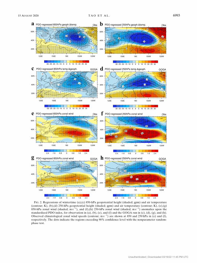
FIG. 2. Regressions of wintertime (a),(c) 850-hPa geopotential height (shaded; gpm) and air temperature

(contour; K), (b),(d) 250-hPa geopotential height (shaded; gpm) and air temperature (contour; K), (e),(g)

850-hPa zonal wind (shaded; m s21), and (f),(h) 250-hPa zonal wind (shaded; m s21) anomalies upon the

standardized PDO index, for observation in (a), (b), (e), and (f) and the GOGA run in (c), (d), (g), and (h).

Observed climatological zonal wind speeds (contour; m s21) are shown at 850 and 250 hPa in (e) and (f),

respectively. The dots indicate the regions exceeding 90% confidence level with the nonparameter random-

phase test.

15 AUGUST 2020 TAO ET AL . 6993

Unauthenticated | Downloaded 03/19/22 11:45 PM UTC

cooling over the western-to-middle North Pacific; at

250 hPa (Fig. 4b), the anomalous geopotential low over

the northeastern North Pacific is retained, while the

cooling temperature anomalies turn to be anomalous

warming. Accordingly, the enhanced westerly winds

appear in the exit region of the westerly jet in both the

lower and upper troposphere (Figs. 4e,f). The geo-

potential height anomalies also display an equivalent

barotropic vertical structure (Fig. 5a) with maximal

amplitude at 300 hPa, as in the GOGA run, despite their

smaller amplitudes and slight northward shifting. The

westerly jet is also accelerated throughout the whole

layer as in the GOGA run but with a weaker strength

(Fig. 5b). These results indicate that the removal of

midlatitudeNorth Pacific SST variabilities only weakens

the amplitudes of the PDO-related atmospheric anom-

alies over North Pacific, without largely altering their

spatial patterns.

To what degree the amplitude of atmospheric re-

sponse is reduced by the removal of the midlatitude

North Pacific SST variabilities can be further identified

by calculating the regressions of differences between the

GOGAand xNPOGA runs upon the PDO standardized

index. As shown in Figs. 4c and 4d, the cooling SST

anomalies in the midlatitude North Pacific tend to induce

atmospheric anomalies with a cold/trough structure in the

FIG. 3. Latitude–altitude sections averaged between 1408E and 1208W of regressions of wintertime (a),(c) geo-

potential height (shaded; gpm) and air temperature (contour; K), and (b),(d) zonal wind (shaded; m s21) on the

standardized PDO index, for (top) observation and (bottom) the GOGA run. Observed and GOGA-simulated

cimatological zonal wind speeds (contour; m s21) are shown in (b) and (d), respectively. The dots indicate the

regions exceeding 90% confidence level with the nonparameter random-phase test.

6994 JOURNAL OF CL IMATE VOLUME 33

Unauthenticated | Downloaded 03/19/22 11:45 PM UTC

FIG. 4. Regressions of xNPOGA-simulated wintertime (a) 850-hPa geopotential height (shaded; gpm) and air

temperature (contour; K), (b) 250-hPa geopotential height (shaded; gpm) and air temperature (contour; K),

(e) 850-hPa zonal wind (shaded; m s21), and (f) 250-hPa zonal wind (shaded; m s21) anomalies upon the stan-

dardized PDO index. (c),(d),(g),(h) As in (a), (b), (e), and (f), respectively, but for the regressions of differences

betweenGOGAand xNPOGA (GOGA2 xNPOGA). The xNPOGA-simulated climatological zonal wind speeds

(contour; m s21) at 850 and 250 hPa are shown in (e),(g) and in (f),(h), respectively. The dots indicate the regions

exceeding 90% confidence level with the nonparameter random-phase test.

15 AUGUST 2020 TAO ET AL . 6995

Unauthenticated | Downloaded 03/19/22 11:45 PM UTC

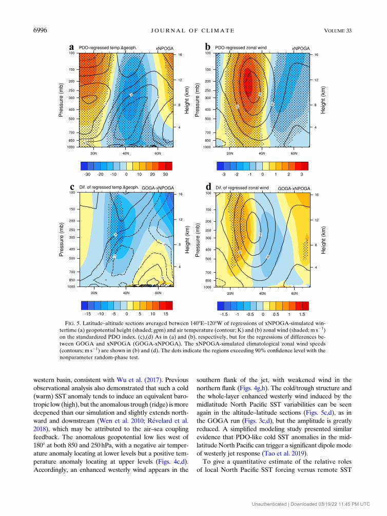
western basin, consistent with Wu et al. (2017). Previous

observational analysis also demonstrated that such a cold

(warm) SST anomaly tends to induce an equivalent baro-

tropic low (high), but the anomalous trough (ridge) ismore

deepened than our simulation and slightly extends north-

ward and downstream (Wen et al. 2010; Révelard et al.

2018), which may be attributed to the air–sea coupling

feedback. The anomalous geopotential low lies west of

1808 at both 850 and 250hPa, with a negative air temper-

ature anomaly locating at lower levels but a positive tem-

perature anomaly locating at upper levels (Figs. 4c,d).

Accordingly, an enhanced westerly wind appears in the

southern flank of the jet, with weakened wind in the

northern flank (Figs. 4g,h). The cold/trough structure and

the whole-layer enhanced westerly wind induced by the

midlatitude North Pacific SST variabilities can be seen

again in the altitude–latitude sections (Figs. 5c,d), as in

the GOGA run (Figs. 3c,d), but the amplitude is greatly

reduced. A simplified modeling study presented similar

evidence that PDO-like cold SST anomalies in the mid-

latitude North Pacific can trigger a significant dipole mode

of westerly jet response (Tao et al. 2019).

To give a quantitative estimate of the relative roles

of local North Pacific SST forcing versus remote SST

FIG. 5. Latitude–altitude sections averaged between 1408E–1208W of regressions of xNPOGA-simulated win-

tertime (a) geopotential height (shaded; gpm) and air temperature (contour; K) and (b) zonal wind (shaded; m s21)

on the standardized PDO index. (c),(d) As in (a) and (b), respectively, but for the regressions of differences be-

tween GOGA and xNPOGA (GOGA-xNPOGA). The xNPOGA-simulated climatological zonal wind speeds

(contours; m s21) are shown in (b) and (d). The dots indicate the regions exceeding 90% confidence level with the

nonparameter random-phase test.

6996 JOURNAL OF CL IMATE VOLUME 33

Unauthenticated | Downloaded 03/19/22 11:45 PM UTC

forcing in the formation of the PDO-related cold/trough

structure, we define and calculate a ratio of the North

Pacific SST anomaly-induced PDO-regressed geopotential

height anomalies over those induced by the global SST

anomalies, that is, (GOGA 2 xNPOGA)/GOGA for

PDO-regressed geopotential height anomalies. In terms

of the vertical distributions of regresssed geopotential

height anomalies (Figs. 3c and 5c), the ratio is averaged

over ranges from 1000 to 100 hPa in vertical direction

and from 308 to 408N in the meridional direction, cov-

ering most of the regions with negative anomalies ex-

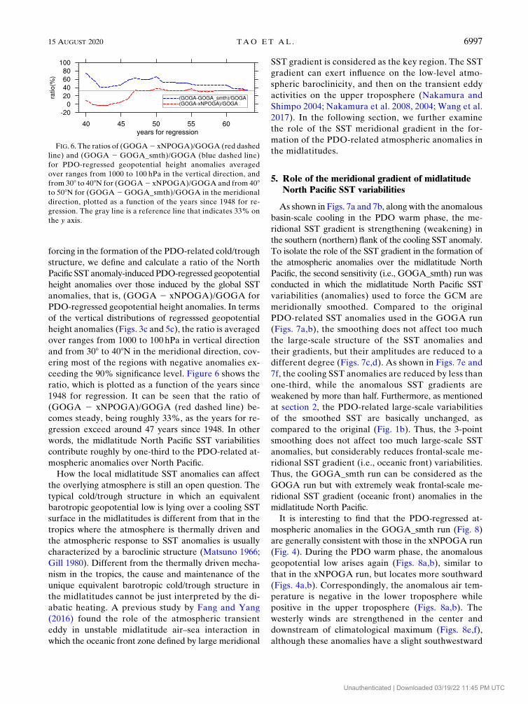
ceeding the 90% significance level. Figure 6 shows the

ratio, which is plotted as a function of the years since

1948 for regression. It can be seen that the ratio of

(GOGA 2 xNPOGA)/GOGA (red dashed line) be-

comes steady, being roughly 33%, as the years for re-

gression exceed around 47 years since 1948. In other

words, the midlatitude North Pacific SST variabilities

contribute roughly by one-third to the PDO-related at-

mospheric anomalies over North Pacific.

How the local midlatitude SST anomalies can affect

the overlying atmosphere is still an open question. The

typical cold/trough structure in which an equivalent

barotropic geopotential low is lying over a cooling SST

surface in the midlatitudes is different from that in the

tropics where the atmosphere is thermally driven and

the atmospheric response to SST anomalies is usually

characterized by a baroclinic structure (Matsuno 1966;

Gill 1980). Different from the thermally driven mecha-

nism in the tropics, the cause and maintenance of the

unique equivalent barotropic cold/trough structure in

the midlatitudes cannot be just interpreted by the di-

abatic heating. A previous study by Fang and Yang

(2016) found the role of the atmospheric transient

eddy in unstable midlatitude air–sea interaction in

which the oceanic front zone defined by large meridional

SST gradient is considered as the key region. The SST

gradient can exert influence on the low-level atmo-

spheric baroclinicity, and then on the transient eddy

activities on the upper troposphere (Nakamura and

Shimpo 2004; Nakamura et al. 2008, 2004; Wang et al.

2017). In the following section, we further examine

the role of the SST meridional gradient in the for-

mation of the PDO-related atmospheric anomalies in

the midlatitudes.

5. Role of the meridional gradient of midlatitudeNorth Pacific SST variabilities

As shown in Figs. 7a and 7b, along with the anomalous

basin-scale cooling in the PDO warm phase, the me-

ridional SST gradient is strengthening (weakening) in

the southern (northern) flank of the cooling SST anomaly.

To isolate the role of the SST gradient in the formation of

the atmospheric anomalies over the midlatitude North

Pacific, the second sensitivity (i.e., GOGA_smth) run was

conducted in which the midlatitude North Pacific SST

variabilities (anomalies) used to force the GCM are

meridionally smoothed. Compared to the original

PDO-related SST anomalies used in the GOGA run

(Figs. 7a,b), the smoothing does not affect too much

the large-scale structure of the SST anomalies and

their gradients, but their amplitudes are reduced to a

different degree (Figs. 7c,d). As shown in Figs. 7e and

7f, the cooling SST anomalies are reduced by less than

one-third, while the anomalous SST gradients are

weakened by more than half. Furthermore, as mentioned

at section 2, the PDO-related large-scale variabilities

of the smoothed SST are basically unchanged, as

compared to the original (Fig. 1b). Thus, the 3-point

smoothing does not affect too much large-scale SST

anomalies, but considerably reduces frontal-scale me-

ridional SST gradient (i.e., oceanic front) variabilities.

Thus, the GOGA_smth run can be considered as the

GOGA run but with extremely weak frontal-scale me-

ridional SST gradient (oceanic front) anomalies in the

midlatitude North Pacific.

It is interesting to find that the PDO-regressed at-

mospheric anomalies in the GOGA_smth run (Fig. 8)

are generally consistent with those in the xNPOGA run

(Fig. 4). During the PDO warm phase, the anomalous

geopotential low arises again (Figs. 8a,b), similar to

that in the xNPOGA run, but locates more southward

(Figs. 4a,b). Correspondingly, the anomalous air tem-

perature is negative in the lower troposphere while

positive in the upper troposphere (Figs. 8a,b). The

westerly winds are strengthened in the center and

downstream of climatological maximum (Figs. 8e,f),

although these anomalies have a slight southwestward

FIG. 6. The ratios of (GOGA2 xNPOGA)/GOGA (red dashed

line) and (GOGA 2 GOGA_smth)/GOGA (blue dashed line)

for PDO-regressed geopotential height anomalies averaged

over ranges from 1000 to 100 hPa in the vertical direction, and

from 308 to 408N for (GOGA2 xNPOGA)/GOGA and from 408to 508N for (GOGA 2GOGA_smth)/GOGA in the meridional

direction, plotted as a function of the years since 1948 for re-

gression. The gray line is a reference line that indicates 33% on

the y axis.

15 AUGUST 2020 TAO ET AL . 6997

Unauthenticated | Downloaded 03/19/22 11:45 PM UTC

shift as compared to those in the xNPOGArun (Figs. 4e,f).

Furthermore, as shown in Figs. 9a and 9b, both the

anomalous geopotential low and the strengthened zonal

wind demonstrate again equivalent barotropic vertical

structures that are quite similar to those in the xNPOGA

run, not only in their distributions but their amplitudes.

The similarity of atmospheric responses between the

GOGA_smth and xNPOGA runs indicates that the re-

spective removal of the North Pacific SST variabilities and

their frontal-scale meridional gradients exerts an equiva-

lent effect on the atmosphere, especially in the upper

troposphere.

Similarly, by looking at the regression of difference

between the GOGA and GOGA_smth runs upon the

standardized PDO index, the effect of the frontal-scale

SST gradient variabilities can be seen more clearly. As

shown in Figs. 8c and 8d, the meridional SST gradient

anomalies in North Pacific tend to considerably induce

an anomalous geopotential low over the northeastern

North Pacific. Besides, they also strengthen the western

part of the GOGA’s cold/trough structure (Figs. 2c,d),

and the anomalous geopotential low in the western basin

is similar to that induced by the North Pacific SST

anomalies (Figs. 4c,d). In the western basin, the westerly

wind is enhanced (decreased) in the southern (northern)

flank of the jet, while it is enhanced east of 1808,downstream of the jet (Figs. 8g,h). The latitude–altitude

distributions exhibit that the SST gradient anomalies-

induced geopotential height and zonal wind anomalies

are equivalent barotropic (Figs. 9c,d). Compared to

FIG. 7. Regressions of wintertime (a),(c) SST (K) and (b),(d) SST gradient [K (110 km)21] anomalies upon the

standardized PDO index used in the (a),(b) GOGA and (c),(d) GOGA_smth runs. (e),(f) The regressions of

differences between GOGA and GOGA_smth (GOGA2 GOGA_smth), respectively, in which the contours are

exactly the same as the shades in (a) and (b), respectively. The dots indicate the regions exceeding 90% confidence

level with the nonparameter random-phase test.

6998 JOURNAL OF CL IMATE VOLUME 33

Unauthenticated | Downloaded 03/19/22 11:45 PM UTC

those induced by the North Pacific SST anomalies

(Figs. 5c,d), the atmospheric anomalies by the SST

gradient anomalies (Figs. 9c,d) have the comparable

amplitudes despite their northward shifts in location.

A quantitative relative contribution of the SST

gradient anomalies to the total atmospheric response

is similarly estimated, by calculating the ratio of

(GOGA 2 GOGA_smth)/GOGA for PDO-regressed

geopotential height anomalies averaged over the ranges

from 1000 to 100 hPa in vertical direction and from

408 to 508N in meridional direction, which cover most

of the regions with negative geopotential height anom-

alies exceeding 90% significance level. As shown in

Fig. 6, the relative contribution to the geopotential

FIG. 8. As in Fig. 4, but for the GOGA_smth run and for the regressions of differences between GOGA and

GOGA_smth (GOGA 2 GOGA_smth).

15 AUGUST 2020 TAO ET AL . 6999

Unauthenticated | Downloaded 03/19/22 11:45 PM UTC

height anomalies by the frontal-scale meridional SST

gradient anomalies (blue dashed line) merges with

that by the North Pacific SST anomalies (red dashed

line), as the years for regression exceed 60 years since

1948, although the meridional ranges for averaging

geopotential height anomalies have a slight differ-

ence. Therefore, during the PDO warm phase, the

frontal-scale SST gradient anomalies also contribute

roughly by one-third to the anomalous cold/trough

structure as well as the enhanced westerly wind in the

GOGA run, comparable to what the North Pacific

SST anomalies do. One possible deduction from the

results is that the SST anomalies in the midlatitude

North Pacific affect the atmosphere mainly through

the anomalous meridional SST gradients. In the fol-

lowing section, we further examine possiblemechanisms

and processes by which the midlatitude SST anomalies

affect the atmosphere.

6. Ways the midlatitude North Pacific SSTvariabilities affect the atmosphere

a. Forcing sources of midlatitude seasonal meanatmospheric state

As mentioned in section 4, the midlatitude atmo-

sphere is characterized by abundant synoptic transient

eddy activities due to atmospheric baroclinicity. The

midlatitude SST anomaly may affect the atmosphere

by altering low-level atmospheric baroclinicity. In the

GOGA run, as shown in Figs. 10a and 10b, the clima-

tological meridional air temperature gradient is large

over the Kuroshio–Oyashio Extension (KOE) regions,

FIG. 9. As in Fig. 5, but for the GOGA_smth run and for the regressions of differences between GOGA and

GOGA_smth (GOGA 2 GOGA_smth).

7000 JOURNAL OF CL IMATE VOLUME 33

Unauthenticated | Downloaded 03/19/22 11:45 PM UTC

coinciding with large climatological atmospheric baro-

clinicity represented by Eady growth rate at 850 hPa.

During the PDO warm phase, both the air temperature

gradient and atmospheric baroclinicity are enhanced

downstream of their climatological maximums, with

two branches west of 1808 (Figs. 10a,b), correspondingto the enhanced SST gradient anomalies (Fig. 7b). For

both GOGA minus xNPOGA and GOGA minus

GOGA_smth, the SST and its frontal-scale meridional

gradient anomalies tend to strengthen the atmospheric

baroclinicity between 208 and 408N over the North

Pacific (Figs. 10c–f), when the PDO is in its positive

phase. The former mainly strengthens the southern

branch while the latter mainly strengthens the northern

branch, which is consistent with recent observational

results that the basin-scale SST gradient anomalies in

the central-to-eastern North Pacific could have an im-

pact on the atmosphere comparable to those in the KOE

region (Wang et al. 2017; Révelard et al. 2018). Gan and

Wu (2013) utilized lagged maximum covariance analysis

of observed wintertime storm tracks and SSTs and

proposed that preceding cold SST anomalies in the

western-central North Pacific are associated with the

equatorward shift of atmospheric baroclinicity and

storm track, which is consistent with our simulation

results. Therefore, a strengthened SST gradient caused

FIG. 10. Regressions of wintertime (a) 850-hPa meridional temperature gradient [shaded; K (110 km)21] and

(b) 850-hPa Eady growth rate (shaded; day21) anomalies in the GOGA run upon the standardized PDO index.

Their respective climatologies (contours) are shown in (a) and (b). (c),(d) The corresponding regressions of dif-

ferences between GOGA and xNPOGA (GOGA 2 xNPOGA, and (e),(f) the differences between GOGA and

GOGA_smth (GOGA2GOGA_smth). The contours in (c),(e) and in (d),(f) are exactly the same as the shading in

(a) and (b), respectively. The dots indicate the regions exceeding 90% confidence level with the nonparameter

random-phase test.

15 AUGUST 2020 TAO ET AL . 7001

Unauthenticated | Downloaded 03/19/22 11:45 PM UTC

by the SST anomaly generates a strengthened atmo-

spheric temperature gradient as well as an enhanced

atmospheric baroclinicity, favoring the generation of

more synoptic baroclinic Rossby waves, namely tran-

sient eddies.

The synoptic transient eddy can redistribute heat and

momentum efficiently in the upper troposphere, which is

essential in formation and maintenance of the midlati-

tude eddy-driven jet (Williams 1979; Panetta and Held

1988; Panetta 1993). Following Fang and Yang (2016),

the role of the synoptic transient eddy in the midlati-

tude seasonal-mean atmospheric state can be determined

by the quasigeostrophic potential vorticity (QGPV)

equation:

�›

›t1V

h� =��

1

f=2F1 f 1

›

›p

�f

s1

›F

›p

��

52f›

›p

a

s1

Qd

T

!2 f

›

›p

a

s1

Qeddy

T

!1F

eddy, (1)

where the overbar denotes the seasonal mean, F is

the geopotential height, a is the reciprocal of density,

s1 is the static stability parameter (s1 5 2a› lnu/›p),

and T is the temperature. Also, Qd is the seasonal-

mean diabatic heating, calculated with four compo-

nents of model outputs (vertical diffusion, latent heat

of condensation, longwave and shortwave radiation

heating/cooling); Qeddy and Feddy are two transient

eddy forcing terms, namely the seasonal-mean transient

eddy heating and vorticity forcing term, respectively. They

are basically determined by the convergence of transient

eddy heat and vorticity fluxes, respectively, which can be

expressed asQeddy 52= �V0hT

0 2 ›v0T 0/›p1R/Cppv0T 0,and Feddy 52= �V0

h§0, where the prime denotes the de-

viations from seasonal mean, § is the relative vorticity,R is

the gas constant, and Cp is the specific heat at constant

pressure. Since the low-level atmospheric baroclinicity is

closely related to high-frequency transient eddy activity

(Simmons and Hoskins 1978; Hoskins and James 2014),

the role of synoptic-scale (2–8-day filtered) transient

eddies is only discussed in this study.

On the right-hand side of Eq. (1), there are three

forcing terms that can generate atmospheric potential

vorticity (PV): diabatic heating (F1), transient eddy

heating forcing (F2), and transient eddy vorticity forcing

(F3). The midlatitude seasonal-mean atmospheric state

is driven by both thermal and dynamical forcing. Thus,

the midlatitude SST anomalies can affect the atmo-

sphere through two ways: direct thermal forcing by

diabatic forcing and indirect thermal and dynami-

cal forcing by atmospheric transient eddy activities.

These forcing terms that are associated with PDO are

calculated with daily model output data and presented

in Figs. 11 and 12 . The vertical structure of diabatic

heating and transient eddy forcing terms can be iden-

tified by their zonal averages over the basin-scale

midlatitude North Pacific. For the GOGA run, clima-

tologically (shown with contours in Figs. 11a–c), the

diabatic heating is generally confined to the lower tro-

posphere over the midlatitude North Pacific (Fig. 11a),

while the transient eddy heating has positive centers in

themid- to upper troposphere north of 328Nand negative

centers in the mid- to lower troposphere south of 458N,

forming a baroclinic structure between 328 and 458N(Fig. 11b). Interestingly, the transient eddy vorticity

forcing is characterized by an equivalent barotropic me-

ridional dipole structure in climatology, with larger pos-

itive (negative) centers north (south) of 358N in the upper

troposphere (Fig. 11c).

During the PDO warm phase, diabatic heating

anomalies are basically in phase with its climatology,

mainly confined to the lower troposphere, although

some can penetrate into high-level atmosphere (Fig. 11a).

However, through transient eddy activities, the tran-

sient eddy forcing can influence the mid- to upper

troposphere. The transient eddy heating is enhanced

and shifts southward in the whole troposphere at

around 408N, especially in the mid- to lower tropo-

sphere (Fig. 11b). The transient eddy vorticity forcing

anomaly demonstrates a vertical structure similar to its

climatology, but shifts southward (Fig. 11c). Overall,

the transient eddy forcing is intensified and shifts

southward, corresponding to the atmospheric baroclinicity

anomalies (Fig. 10b). To compare with the anomalous

transient eddy vorticity forcing term F3 (Fig. 12c), we

further calculate the former two forcing terms (F1 and F2)

that are proportional to the vertical gradient of diabatic

heating anomalies and transient eddy heating anomalies,

respectively. Different from the equivalent barotropic

structure of F3 (Fig. 12c), both F1 and F2 display a baro-

clinic structure with a negative (positive) anomaly above

(below) its maximal heating anomaly in the vertical di-

rection, respectively, partly canceling each other out at

around 408N (Figs. 12a,b).

The effects of the midlatitude North Pacific SST

anomalies and their SST gradients on the diabatic

heating, transient eddy heating, and transient eddy

vorticity forcing are also shown. Basically, the anomalies

of those forcing terms induced by the SST anomalies and

by the SST gradient anomalies are similar, and all in

phase with the anomalies from the GOGA run, but their

amplitudes are relatively weak (Figs. 11 and 12). The

transient eddy transport anomalies induced by the SST

anomalies slightly shift southward (Figs. 11e,f), but

are shifted northward by the SST gradient anomalies

7002 JOURNAL OF CL IMATE VOLUME 33

Unauthenticated | Downloaded 03/19/22 11:45 PM UTC

(Figs. 11f,i), corresponding to the shifts of the at-

mospheric low-level temperature gradient and bar-

oclinicity, respectively (Figs. 10c–f). As in the GOGA

run, F1 and F2 induced by the SST anomalies and by

the SST gradient anomalies are both baroclinic, and

partly cancel out each other (Figs. 12d,e,g,h), and only

F3 is equivalent barotropic in the vertical direction

(Figs. 12f,i).

b. Relative contributions of different forcing sources

To quantitatively analyze the relative contributions of

anomalous diabatic heating, transient eddy heating, and

FIG. 11. Latitude–altitude sections averaged between 1408E and 1208W of regressions of wintertime (a) diabatic heating (shaded;

K day21), (b) transient eddy heating (shaded; K day21), and (c) transient eddy vorticity forcing (shaded; 10211 s22) anomalies in the

GOGA run upon the standardized PDO index. Their respective climatologies (contours) are shown in (a)–(c). (d)–(f) The corresponding

regressions of differences between GOGA and xNPOGA (GOGA 2 xNPOGA), and (g)–(i) the differences between GOGA and

GOGA_smth (GOGA2GOGA_smth). The contours in (d)–(f) and in (g)–(i) are exactly the same as the shades in (a)–(c), respectively.

The dots indicate the regions exceeding 90% confidence level with the nonparameter random-phase test.

15 AUGUST 2020 TAO ET AL . 7003

Unauthenticated | Downloaded 03/19/22 11:45 PM UTC

transient eddy vorticity forcing to the winter mean atmo-

spheric anomalies, the tendency of geopotential height

anomalies induced by those forcing anomalies is deter-

mined by the following relation (Fang and Yang 2016):�1

f=2 1 f

›

›p

�1

s1

›

›p

���›DF

›t

�}

2f›

›p

a

s1

DQd

T

!2 f

›

›p

a

s1

DQeddy

T

!1DF

eddy, (2)

where D denotes the anomaly. Given the forcing terms,

the tendency of geopotential height anomalies can be

numerically solved with the successive overrelaxation

(SOR) method. The settings of boundary conditions are

important and may disturb the solution as the SOR

method is applied. The effect of horizontal boundary

condition is small, which can be set as�›F

›t

�2:58S

5 0,›

›y

�›F

›t

�908N

5 0, (3)

FIG. 12. As in Fig. 11, but for the forcing terms (10211 s22) induced by (a),(d),(g) diabatic heating anomalies (F1), (b),(e),(h) transient eddy

heating anomalies (F2), and (c),(f),(i) transient eddy vorticity forcing anomalies (F3).

7004 JOURNAL OF CL IMATE VOLUME 33

Unauthenticated | Downloaded 03/19/22 11:45 PM UTC

in the y direction. A cycling boundary is applied in the x

direction. Following Lau and Holopainen (1984), we set

the vertical boundary conditions for Qd and Qeddy as�›

›p

�›F

›t

��1000 hPa/100 hPa

52R

pQ

1000hPa/100 hPa, (4)

at 1000 and 100hPa, respectively. For Feddy, they are

set as �›

›p

�›F

›t

��1000 hPa/100 hPa

5 0: (5)

The vertical boundary conditions may have some effect

on the geopotential tendencies in the stratosphere in-

duced by Qd and Qeddy, which are supposed to vanish

there. The geopotential height tendency induced by the

diabatic heating, transient eddy heating, and transient

eddy vorticity forcing, respectively, is calculated and

shown in Fig. 13.

In the GOGA run, the anomalous diabatic heating

tends to induce geopotential tendency anomaly with a

tripole structure in vertical direction at around 408N(Fig. 13a), while the geopotential tendency induced by

the anomalous transient eddy heating features a dipole

in the vertical (Fig. 13b). Therefore, the geopotential

responses to both thermal forcing terms are baroclinic.

Nevertheless, the geopotential tendency induced by the

anomalous transient eddy vorticity forcing is equivalent

barotropic, characterized by a negative geopotential

height tendency anomaly at around 408N (Fig. 13c),

corresponding to the anomalous geopotential low in

Fig. 3c. Therefore, the transient eddy vorticity forcing

is more important than other two thermal forcing terms

in the formation of the cold/trough structure, as found

by Fang and Yang (2016). As for the GOGA minus

xNPOGA and GOGAminus GOGA_smth cases, all of

the geopotential tendencies induced by diabatic heating

forcing and transient eddy heating forcing are also bar-

oclinic (Figs. 13d,e,g,h). Only the geopotential tendency

induced by transient vorticity forcing is equivalent bar-

otropic in both GOGA 2 xNPOGA and GOGA 2GOGA_smth, and has a southward shift in the former

case but a northward shift in the latter case, corre-

sponding to the anomalous geopotential height in Figs. 5c

and 9c, respectively.

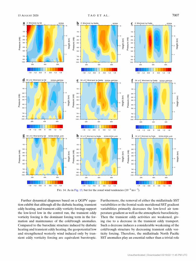
In terms of the geostrophic relationship, the zonal

wind tendency can be derived from the geopotential

height tendency. The zonal wind is increased in the

southern flank of the geopotential low, while decreased

in its northern flank. Again, the zonal wind tendency

induced only by the transient eddy vorticity forcing is

equivalent barotropic (Fig. 14c), while that induced by

either the diabatic heating or the transient eddy heating

is baroclinic in the GOGA run (Figs. 14a,b). As

for the GOGA minus xNPOGA and GOGA minus

GOGA_smth cases, the zonal wind tendency induced

by those terms shows similar structure but with weaker

amplitude, and southward shift in the GOGA minus

xNPOGA case and northward shift in the GOGAminus

GOGA_smth case (Figs. 14d–i). The equivalent baro-

tropic positive zonal wind tendency induced by the

transient eddy vorticity forcing in the GOGA, GOGA

minus xNPOGA, and GOGAminus GOGA_smth cases

corresponds to the enhanced westerly wind, as shown in

Figs. 3d, 5d, and 9d, respectively.

Therefore, the above results indicate that the tran-

sient eddy vorticity forcing is a key dynamical process

for the midlatitude North Pacific SST and its gradient

variabilities to affect the atmosphere. Moreover, the

contrast among different runs indicates that large-scale

SST variabilities in the midlatitude North Pacific mainly

affect the diabatic heating, while the similarity among

different runs implies again that the frontal-scale SST

meridional gradient is the key for the midlatitude North

Pacific SST anomalies to affect the atmosphere in which

the transient eddy vorticity forcing is a key player.

7. Conclusions and discussion

The PDO is the dominant decadal-to-interdecadal

climate variability in the North Pacific air–sea system.

During the PDO warm phase, the anomalous winter-

time air–sea system of the midlatitude North Pacific is

characterized by a cold/trough structure in observation;

that is, an anomalous equivalent barotropic geopotential

low lies upon the negative SST anomaly. Forced by long-

term observed global SST in a control run, the typical

wintertime cold/trough structure over the midlatitude

North Pacific is captured by an atmospheric GCM

(GFDL AM2.1), although simulated amplitudes of the

anomalous trough and associated strengthened westerly

wind are weaker than the observed, which may be at-

tributable to the lack of air–sea coupling. To identify the

impact of the midlatitude oceanic thermal condition on

the atmosphere, the SST variabilities in the midlatitude

North Pacific are removed by simply setting the SST

there as climatology in the first sensitivity run. The at-

mospheric response also shows an equivalent barotropic

cold/trough structure in the vertical direction. As for the

anomalous amplitude, the lack of the midlatitude North

Pacific SST variabilities tends to reduce the atmospheric

response by roughly one-third. Therefore, the midlati-

tude North Pacific SST anomalies make a considerable

(approximately one-third) contribution to the PDO-related

cold/trough anomalies, although most of those atmo-

spheric anomalies are determined by the SST variabilities

15 AUGUST 2020 TAO ET AL . 7005

Unauthenticated | Downloaded 03/19/22 11:45 PM UTC

outside of the midlatitude North Pacific, especially by the

tropical Pacific SST variabilities.

Different from the thermally driven mechanism in-

duced by deep convection in the tropics, the diabatic

heating is mainly confined to the low-level troposphere

in the midlatitudes. The typical cold/trough structure

cannot be explained by only thermal processes. During

the PDO warm phase, the meridional SST gradient is

anomalously strengthened in the southern flank of the

cooling SST anomaly. In the second sensitivity run, the

frontal-scale meridional SST gradient variabilities in the

North Pacific are sharply smoothed, while the large-

scale SST variabilities there are kept. In this case, the

simulated PDO-related cold/trough anomalies are also

reduced by nearly one-third. Therefore, the frontal-

scale meridional SST gradient (oceanic front) is essen-

tial in the process of the midlatitude SST anomaly’s

impact on the atmosphere above.

FIG. 13. As in Fig. 11, but for the geopotential tendencies (1024 m2 s23) induced by (a),(d),(g) diabatic heating anomalies (F1), (b),(e),(h)

transient eddy heating anomalies (F2), and (c),(f),(i) transient eddy vorticity forcing anomalies (F3).

7006 JOURNAL OF CL IMATE VOLUME 33

Unauthenticated | Downloaded 03/19/22 11:45 PM UTC

Further dynamical diagnoses based on a QGPV equa-

tion exhibit that although all the diabatic heating, transient

eddy heating, and transient eddy vorticity forcings support

the low-level low in the control run, the transient eddy

vorticity forcing is the dominant forcing term in the for-

mation and maintenance of the cold/trough anomalies.

Compared to the baroclinic structure induced by diabatic

heating and transient eddy heating, the geopotential low

and strengthened westerly wind induced only by tran-

sient eddy vorticity forcing are equivalent barotropic.

Furthermore, the removal of either the midlatitude SST

variabilities or the frontal-scale meridional SST gradient

variabilities primarily decreases the low-level air tem-

perature gradient as well as the atmospheric baroclinicity.

Then the transient eddy activities are weakened, giv-

ing rise to a decrease in the transient eddy transport.

Such a decrease induces a considerable weakening of the

cold/trough structure by decreasing transient eddy vor-

ticity forcing. Therefore, the midlatitude North Pacific

SST anomalies play an essential rather than a trivial role

FIG. 14. As in Fig. 13, but for the zonal wind tendencies (1026 m s22).

15 AUGUST 2020 TAO ET AL . 7007

Unauthenticated | Downloaded 03/19/22 11:45 PM UTC

in the winter atmospheric anomalies associated with

PDO, in which the frontal-scale meridional SST gradient

(oceanic front) and synoptic transient eddy dynamical

feedback are key players.

As the transient eddy activities are important in the

midlatitude air–sea interaction, finer-resolution models

can be better in resolving storm track. Thus, a compar-

ison among different models with diverse resolution is

needed. Furthermore, the seasonal-mean relationship

between the SST and the atmosphere identified in this

study is simultaneous, in terms of AMIP-like experi-

ments. The lead–lag relationships, especially when the

SST anomalies lead the atmospheric anomalies, need to

be further examined with coupled ocean–atmosphere

model experiments.

Acknowledgments. This work is supported by the

National Natural Science Foundation of China (Grant

41621005). We are also grateful for support from the

Jiangsu Collaborative Innovation Center for Climate

Change and the program B for Outstanding PhD can-

didate of Nanjing University.

REFERENCES

Anderson, J. L., and Coauthors, 2004: The new GFDL global at-

mosphere and land model AM2–LM2: Evaluation with pre-

scribed SST simulations. J. Climate, 17, 4641–4673, https://

doi.org/10.1175/JCLI-3223.1.

Battisti, D. S., U. S. Bhatt, andM. A. Alexander, 1995: Amodeling

study of the interannual variability in the wintertime North

Atlantic Ocean. J. Climate, 8, 3067–3083, https://doi.org/

10.1175/1520-0442(1995)008,3067:AMSOTI.2.0.CO;2.

Cayan, D. R., 1992a: Latent and sensible heat flux anomalies over

the northern oceans: The connection to monthly atmospheric

circulation. J. Climate, 5, 354–369, https://doi.org/10.1175/1520-

0442(1992)005,0354:LASHFA.2.0.CO;2.

——, 1992b: Latent and sensible heat flux anomalies over the

northern oceans: Driving the sea surface temperature. J. Phys.

Oceanogr., 22, 859–881, https://doi.org/10.1175/1520-0485(1992)

022,0859:LASHFA.2.0.CO;2.

Chen, Q., H. Hu, X. Ren, and X.-Q. Yang, 2019: Numerical

simulation of midlatitude upper-level zonal wind response

to the change of North Pacific subtropical front strength.

J. Geophys. Res. Atmos., 124, 4891–4912, https://doi.org/10.1029/2018JD029589.

Chu, C.-J., X.-Q. Yang, X.-J. Ren, and T.-J. Zhou, 2013: Response

of Northern Hemisphere storm tracks to Indian-western

Pacific Ocean warming in atmospheric general circulation

models. Climate Dyn., 40, 1057–1070, https://doi.org/10.1007/

s00382-013-1687-y.

Delworth, T. L., and R. J. Greatbatch, 2000: Multidecadal ther-

mohaline circulation variability driven by atmospheric surface

flux forcing. J. Climate, 13, 1481–1495, https://doi.org/10.1175/

1520-0442(2000)013,1481:MTCVDB.2.0.CO;2.

Deser, C., and M. L. Blackmon, 1993: Surface climate variations

over the North Atlantic Ocean during winter: 1900–1989.

J. Climate, 6, 1743–1753, https://doi.org/10.1175/1520-0442(1993)

006,1743:SCVOTN.2.0.CO;2.

——, G. Magnusdottir, R. Saravanan, and A. Phillips, 2004: The

effects of North Atlantic SST and sea ice anomalies on the

winter circulation in CCM3. Part II: Direct and indirect com-

ponents of the response. J. Climate, 17, 877–889, https://doi.org/

10.1175/1520-0442(2004)017,0877:TEONAS.2.0.CO;2.

Dickson, R., J. Lazier, J. Meincke, and P. Rhines, 1996: Long-

term coordinated changes in the convective activity of the

North Atlantic.Decadal Climate Variability: Dynamics and

Predictability, D. L. T. Anderson and J. Willebrand, Eds.,

Springer, 211–261.

Duchon, C. E., 1979: Lanczos filtering in one and two dimen-

sions. J. Appl. Meteor., 18, 1016–1022, https://doi.org/10.1175/

1520-0450(1979)018,1016:LFIOAT.2.0.CO;2.

Ebisuzaki, W., 1997: A method to estimate the statistical significance

of a correlation when the data are serially correlated. J. Climate,

10, 2147–2153, https://doi.org/10.1175/1520-0442(1997)010,2147:

AMTETS.2.0.CO;2.

Enfield, D. B., and A. M. Mestas-Nuñez, 1999: Multiscale vari-

abilities in global sea surface temperatures and their rela-

tionships with tropospheric climate patterns. J. Climate, 12,

2719–2733, https://doi.org/10.1175/1520-0442(1999)012,2719:

MVIGSS.2.0.CO;2.

Fang, J.-B., and X.-Q. Yang, 2016: Structure and dynamics of decadal

anomalies in the wintertime midlatitude North Pacific ocean–

atmosphere system. Climate Dyn., 47, 1989–2007, https://doi.org/

10.1007/s00382-015-2946-x.

Feliks, Y., M. Ghil, and E. Simonnet, 2004: Low-frequency vari-

ability in the midlatitude atmosphere induced by an oceanic

thermal front. J. Atmos. Sci., 61, 961–981, https://doi.org/

10.1175/1520-0469(2004)061,0961:LVITMA.2.0.CO;2.

——, ——, and ——, 2007: Low-frequency variability in the midlati-

tude baroclinic atmosphere induced by an oceanic thermal front.

J. Atmos. Sci., 64, 97–116, https://doi.org/10.1175/JAS3780.1.

Francis, R., and S. Hare, 1997: Regime scale climate forcing of

salmon populations in the Northeast Pacific—Some new

thoughts and findings. Estuarine and Ocean Survival of

Northeastern Pacific Salmon: Proceedings of the Workshop,

NOAA Tech. Memo. NMFSNWFSC-29, 113–128.

Frankignoul, C., P. Müller, and E. Zorita, 1997: A simple model of

the decadal response of the ocean to stochastic wind forcing.

J. Phys. Oceanogr., 27, 1533–1546, https://doi.org/10.1175/

1520-0485(1997)027,1533:ASMOTD.2.0.CO;2.

Gan, B., and L. Wu, 2013: Seasonal and long-term coupling be-

tween wintertime storm tracks and sea surface temperature in

the North Pacific. J. Climate, 26, 6123–6136, https://doi.org/

10.1175/JCLI-D-12-00724.1.

Gates,W.L., 1992:AMIP: TheAtmosphericModel Intercomparison

Project.Bull. Amer. Meteor. Soc., 73, 1962–1970, https://doi.org/

10.1175/1520-0477(1992)073,1962:ATAMIP.2.0.CO;2.

Gill, A. E., 1980: Some simple solutions for heat-induced tropical

circulation. Quart. J. Roy. Meteor. Soc., 106, 447–462, https://

doi.org/10.1002/qj.49710644905.

Hasselmann, K., 1976: Stochastic climate models part I. Theory.

Tellus, 28, 473–485, https://doi.org/10.3402/tellusa.v28i6.11316.

Hoskins, B. J., and D. J. Karoly, 1981: The steady linear re-

sponse of a spherical atmosphere to thermal and orographic

forcing. J. Atmos. Sci., 38, 1179–1196, https://doi.org/10.1175/

1520-0469(1981)038,1179:TSLROA.2.0.CO;2.

——, and I. N. James, 2014: Fluid Dynamics of the Mid-Latitude

Atmosphere. John Wiley & Sons, 432 pp.

Hurrell, J. W., 1995: Decadal trends in the North Atlantic oscilla-

tion: Regional temperatures and precipitation. Science, 269,

676–679, https://doi.org/10.1126/science.269.5224.676.

7008 JOURNAL OF CL IMATE VOLUME 33

Unauthenticated | Downloaded 03/19/22 11:45 PM UTC

Kalnay, E., and Coauthors, 1996: The NCEP/NCAR 40-Year

Reanalysis Project.Bull. Amer. Meteor. Soc., 77, 437–471, https://

doi.org/10.1175/1520-0477(1996)077,0437:TNYRP.2.0.CO;2.

Kanamitsu, M., W. Ebisuzaki, J. Woollen, S.-K. Yang, J. J. Hnilo,

M. Fiorino, and G. L. Potter, 2002: NCEP–DOE AMIP-II

Reanalysis (R-2). Bull. Amer. Meteor. Soc., 83, 1631–1644,

https://doi.org/10.1175/BAMS-83-11-1631.

Kushnir, Y., 1994: Interdecadal variations in North Atlantic Sea

surface temperature and associated atmospheric conditions.

J. Climate, 7, 141–157, https://doi.org/10.1175/1520-0442(1994)

007,0141:IVINAS.2.0.CO;2.

——, and N.-C. Lau, 1992: The general circulation model response

to a North Pacific SST anomaly: Dependence on time scale

and pattern polarity. J. Climate, 5, 271–283, https://doi.org/

10.1175/1520-0442(1992)005,0271:TGCMRT.2.0.CO;2.

——,and I.M.Held, 1996:Equilibriumatmospheric response toNorth

Atlantic SST anomalies. J. Climate, 9, 1208–1220, https://doi.org/

10.1175/1520-0442(1996)009,1208:EARTNA.2.0.CO;2.

Lau, N.-C., and E. O. Holopainen, 1984: Transient eddy forcing

of the time-mean flow as identified by geopotential ten-

dencies. J. Atmos. Sci., 41, 313–328, https://doi.org/10.1175/

1520-0469(1984)041,0313:TEFOTT.2.0.CO;2.

Liu, C.-J., X.-J. Ren, and X.-Q. Yang, 2014: Mean flow-storm track

relationship and Rossby wave breaking in two types of El-

Niño. Adv. Atmos. Sci., 31, 197–210, https://doi.org/10.1007/

s00376-013-2297-7.

Liu, Z.-Y., andL.-X.Wu, 2004:Atmospheric response toNorth Pacific

SST: The role of ocean–atmosphere coupling. J. Climate, 17,

1859–1882, https://doi.org/10.1175/1520-0442(2004)017,1859:

ARTNPS.2.0.CO;2.

——, and E. Di Lorenzo, 2018: Mechanisms and predictability of

Pacific decadal variability.Curr. ClimateChangeRep., 4, 128–144,

https://doi.org/10.1007/s40641-018-0090-5.

Mantua, N. J., and S. R. Hare, 2002: The Pacific decadal oscillation.

J. Oceanogr., 58, 35–44, https://doi.org/10.1023/A:1015820616384.

——,——,Y. Zhang, J.M.Wallace, andR. C. Francis, 1997:APacific

interdecadal climate oscillation with impacts on salmon produc-

tion. Bull. Amer. Meteor. Soc., 78, 1069–1079, https://doi.org/

10.1175/1520-0477(1997)078,1069:APICOW.2.0.CO;2.

Matsuno, T., 1966: Quasi-geostrophic motion in the equatorial

area. J. Meteor. Soc. Japan, 44, 25–43, https://doi.org/10.2151/

jmsj1965.44.1_25.

Miller, A. J., D. R. Cayan, T. P. Barnett, N. E. Graham, and J. M.

Oberhuber, 1994: The 1976–77 climate shift of the Pacific Ocean.

Oceanography, 7, 21–26, https://doi.org/10.5670/oceanog.1994.11.

Minobe, S., 1997: A 50–70 year climatic oscillation over the North

Pacific and North America. Geophys. Res. Lett., 24, 683–686,

https://doi.org/10.1029/97GL00504.

——, A. Kuwano-Yoshida, N. Komori, S.-P. Xie, and R. J. Small,

2008: Influence of theGulf Stream on the troposphere.Nature,

452, 206–209, https://doi.org/10.1038/nature06690.Nakamura, H., and A. Shimpo, 2004: Seasonal variations in the

Southern Hemisphere storm tracks and jet streams as revealed

in a reanalysis dataset. J. Climate, 17, 1828–1844, https://doi.org/

10.1175/1520-0442(2004)017,1828:SVITSH.2.0.CO;2.

——, T. Sampe, Y. Tanimoto, and A. Shimpo, 2004: Observed

associations among storm tracks, jet streams and midlati-

tude oceanic fronts. Earth’s Climate: The Ocean–Atmosphere

Interaction,Geophys. Monogr., Vol. 147, American Geophysical

Union, 329–345.

——, ——, A. Goto, W. Ohfuchi, and S.-P. Xie, 2008: On the

importance of midlatitude oceanic frontal zones for the

mean state and dominant variability in the tropospheric

circulation. Geophys. Res. Lett., 35, L15709, https://doi.org/

10.1029/2008GL034010.

Newman, M., and Coauthors, 2016: The Pacific decadal oscillation,

revisited. J. Climate, 29, 4399–4427, https://doi.org/10.1175/

JCLI-D-15-0508.1.

Nitta, T., and S. Yamada, 1989: Recent warming of tropical sea

surface temperature and its relationship to the Northern

Hemisphere circulation. J. Meteor. Soc. Japan, 67, 375–383,

https://doi.org/10.2151/jmsj1965.67.3_375.

Palmer, T. N., and Z. Sun, 1985: A modelling and observational

study of the relationship between sea surface temperature in

the North-West Atlantic and the atmospheric general circu-

lation. Quart. J. Roy. Meteor. Soc., 111, 947–975, https://

doi.org/10.1002/qj.49711147003.

Panetta, R. L., 1993: Zonal jets in wide baroclinically unstable

regions: Persistence and scale selection. J. Atmos. Sci., 50,

2073–2106, https://doi.org/10.1175/1520-0469(1993)050,2073:

ZJIWBU.2.0.CO;2.

——, and I. M. Held, 1988: Baroclinic eddy fluxes in a one-

dimensional model of quasi-geostrophic turbulence. J. Atmos.

Sci., 45, 3354–3365, https://doi.org/10.1175/1520-0469(1988)

045,3354:BEFIAO.2.0.CO;2.

Peng, S.-L., and J. S. Whitaker, 1999: Mechanisms determining the

atmospheric response to midlatitude SST anomalies. J. Climate,

12, 1393–1408, https://doi.org/10.1175/1520-0442(1999)012,1393:

MDTART.2.0.CO;2.

——, L. A. Mysak, J. Derome, H. Ritchie, and B. Dugas, 1995:

The differences between early and midwinter atmospheric

responses to sea surface temperature anomalies in the

northwest Atlantic. J. Climate, 8, 137–157, https://doi.org/

10.1175/1520-0442(1995)008,0137:TDBEAM.2.0.CO;2.

——, W. A. Robinson, and M. P. Hoerling, 1997: The modeled

atmospheric response to midlatitude SST anomalies and its

dependence on background circulation states. J. Climate, 10,

971–987, https://doi.org/10.1175/1520-0442(1997)010,0971:

TMARTM.2.0.CO;2.

Pitcher, E. J., M. L. Blackmon, G. T. Bates, and S. Muñoz, 1988:The effect of North Pacific Sea surface temperature anomalies on

the January climate of a general circulation model. J. Atmos. Sci.,

45, 173–188, https://doi.org/10.1175/1520-0469(1988)045,0173:

TEONPS.2.0.CO;2.

Ren, X.-J., X.-Q. Yang, and C.-J. Chu, 2010: Seasonal variations of

the synoptic-scale transient eddy activity and polar front jet

over East Asia. J. Climate, 23, 3222–3233, https://doi.org/

10.1175/2009JCLI3225.1.

Révelard, A., C. Frankignoul, and Y.-O. Kwon, 2018: A multi-

variate estimate of the cold season atmospheric response to

North Pacific SST variability. J. Climate, 31, 2771–2796, https://

doi.org/10.1175/JCLI-D-17-0061.1.

Sampe, T., H. Nakamura, A. Goto, and W. Ohfuchi, 2010:

Significance of amidlatitude SST frontal zone in the formation

of a storm track and an eddy-drivenwesterly jet. J. Climate, 23,

1793–1814, https://doi.org/10.1175/2009JCLI3163.1.

Simmons, A. J., and B. J. Hoskins, 1978: The life cycles of some

nonlinear baroclinic waves. J. Atmos. Sci., 35, 414–432,

https://doi.org/10.1175/1520-0469(1978)035,0414:TLCOSN.2.0.CO;2.

Sun, X., L. Tao, and X.-Q. Yang, 2018: The influence of oceanic sto-

chastic forcing on the atmospheric response to midlatitude North

Pacific SST anomalies.Geophys. Res. Lett., 45, 9297–9304, https://

doi.org/10.1029/2018GL078860.

Tao, L., X. Sun, and X.-Q. Yang, 2019: The asymmetric atmospheric

response to the midlatitude North Pacific SST anomalies.

15 AUGUST 2020 TAO ET AL . 7009

Unauthenticated | Downloaded 03/19/22 11:45 PM UTC

J. Geophys. Res. Atmos., 124, 9222–9240, https://doi.org/

10.1029/2019JD030500.

Vallis, G. K., 2006: Atmospheric and Oceanic Fluid Dynamics:

Fundamentals and Large-Scale Circulation. Cambridge

University Press, 745 pp.

Wang, L., X.-Q. Yang, D. Yang, Q. Xie, J. Fang, and X. Sun, 2017:

Two typical modes in the variabilities of wintertime North

Pacific basin-scale oceanic fronts and associated atmospheric

eddy-driven jet. Atmos. Sci. Lett., 18, 373–380, https://doi.org/

10.1002/asl.766.

——, H. Hu, and X. Yang, 2019: The atmospheric responses to the

intensity variability of subtropical front in the wintertime

North Pacific. Climate Dyn., 52, 5623–5639, https://doi.org/

10.1007/S00382-018-4468-9.

Wen, N., Z. Liu, Q. Liu and C. Frankignoul, 2010: Observed at-

mospheric responses to global SST variability modes: A uni-

fied assessment using GEFA. J. Climate, 23, 1739–1759,

https://doi.org/10.1175/2009JCLI3027.1.

Williams, G. P., 1979: Planetary circulations: 2. The Jovian quasi-

geostrophic regime. J. Atmos. Sci., 36, 932–969, https://doi.org/

10.1175/1520-0469(1979)036,0932:PCTJQG.2.0.CO;2.

Wu, B., T. Zhou, and T. Li, 2016: Impacts of the Pacific–Japan and

circumglobal teleconnection patterns on the interdecadal

variability of the East Asian summer monsoon. 29, 3253–3271,

https://doi.org/10.1175/JCLI-D-15-0105.1.

——, ——, and ——, 2017: Atmospheric dynamic and thermo-

dynamic processes driving the western North Pacific anom-

alous anticyclone during El Niño. Part I: Maintenance

mechanisms. J. Climate, 30, 9621–9635, https://doi.org/10.1175/JCLI-D-16-0489.1.

Yao, Y., Z. Zhong, and X.-Q. Yang, 2016: Numerical ex-

periments of the storm track sensitivity to oceanic fron-

tal strength within the Kuroshio/Oyashio Extensions.

J. Geophys. Res. Atmos., 121, 2888–2900, https://doi.org/

10.1002/2015JD024381.

——, ——, ——, and W. Lu, 2017: An observational study of the

North Pacific storm-track impact on the midlatitude oceanic

front. J. Geophys. Res. Atmos., 122, 6962–6975, https://doi.org/

10.1002/2016JD026192.

Zhang, Y., J. M. Wallace, and D. S. Battisti, 1997: ENSO-like inter-

decadal variability: 1900–93. J. Climate, 10, 1004–1020, https://

doi.org/10.1175/1520-0442(1997)010,1004:ELIV.2.0.CO;2.

Zhong, Y., Z. Liu, and R. Jacob, 2008: Origin of Pacific multidecadal

variability in Community Climate System Model, version 3

(CCSM3): A combined statistical and dynamical assessment.

J. Climate, 21, 114–133, https://doi.org/10.1175/2007JCLI1730.1.

Zhu, Y., and X. Yang, 2003: Joint propagating patterns of SST and

SLP anomalies in the North Pacific on bidecadal and penta-

decadal timescales. Adv. Atmos. Sci., 20, 694–710, https://

doi.org/10.1007/BF02915396.

7010 JOURNAL OF CL IMATE VOLUME 33

Unauthenticated | Downloaded 03/19/22 11:45 PM UTC