GIS Ostrava 2008 27. - 30. 1. 2008, Ostrava

1

THE USE OF GIS IN ESTIMATING THE REAL EROSION IN

ZAYANDEHROOD BASIN

Dr Amir Gandomkar

Islamic Azad University – Najafabad Branch

Department: Geography

Islamic Azad university – Najafabad Branch, Najafabad, Isfahan, Iran

E-mail: aagandomkar@yahoo.com

Abstract

Interpolation, the generalization of point data to scatter data, and combining maps are three cases

of important applications of GIS in Climatology studies. In this study, it has been tried to make the

estimation of rain erosion capacity (Fournier Method) more real through using GIS capability in

interpolation and the generalization of point data to scatter data. In Fournier method, the rain erosion

capacity is calculated through the use of two climatic parameters (annual precipitation and the

rainfall mean in the rainiest month of year) and two physiological parameters (the height and slop of

the region).In Fournier method only use means of four parameters, but in this research use the amount

of each parameters in each pixcel of basin and then combin together. The findings of this study

indicated that there is significant difference between these two methods of calculating rain erosion

capacity. Using the means, rain erosion potential was estimated to be almost 121 tones per square

kilometers annually while this amount was estimated to be 267 tones per square kilometers annually

by using GIS capabilities (use the amount of each parameters in each pixcel of basin and then combin

together).

1. Introduction

One of the problems that researchers of geomorphology, climatology and civil are met in landuse

planning, is estimating the real amount of the rain deposition, because in some cases complex factors

should be computed which their assessment is difficult, time consuming and expensive. There are

more than 90 methods to estimate deposition square of an area which is different in accordance with

the type of the deposition in used elements (Gandomkar 2000).

Douglas's Method (Douglas 1973), Musgrave's Method (1947) and Fournier's Method (1960)

(Fournier 1960) are some common examples of estimating deposition. These models have used some

limited factors which are quite simple to obtain or evaluate. In some other methods, various factors are

used, such as: USLE Method (Wishmayer 1947, 1976), EMP Method (Yaroslov Serni 1952)

(Gavrilovic 1988), Fao Method, Estlic Method (Zashar 1982), Psiac Method (PSIAC) and SLEMSA

Method (Ramesht 1996).

Purpose of this research is estimating the real erosion in Zayandehrood basin for loanduse planing,

environmental protection and reduce soil erosian in this basin.

2. MATERIALS AND METHODS

Fournier's Method (1960) estimates amount of annual deposition of a basin with respect to climatic

and morphologic specialties. In this method, two climatic parameters (average annual precipitation and

rainfall mean in the rainiest month of year) and two physiological parameters (The height and slope of

the basin) are used to compute the square of the rain erosion capacity as following (Chorley, Schumm

and Sugden 1985).

Equation (1): 1.56 - tanS) H(0.46Log

P2.65Log Log

2

sQ ×+=ρ

H : Average height of the basin according to meter

S: Average slope of the basin according to degree

GIS Ostrava 2008 27. - 30. 1. 2008, Ostrava

2

P : Average annual precipitation according to mm

Qs: Deposition according to ton in square kilometer in a year

ρ 2: Rainfall mean in the rainiest month of year according to mm (Rafahi 1999)

Fournier studied floating deposition weight for 78 arid or semi arid areas in Tunisia and Algeria which

had a survey from 2460 to 1060000 square kilometer. He showed that there's a meaningful relationship

between the deposition weight and regard monthly rain to average annual (P2ρ

) in areas which

have different unevenness. In this relation, P is the average annually precipitation according to mm

and ρ 2

is the Rainfall mean in the rainiest month of year according to mm. So it's clear that in arid

and semi arid areas which most precipitation of a year happens in one or two special months, the

relation between P2ρ

will increase and the impression amount of this factor in Rain erosion

capacity will increase, too. So the deposition capacity of basin in respect with wet areas will be more

(Chorley, Schumm and Sugden 1985).

In equation (1), average factors are used in basin. This method seem correct when basin is completely

constant and each factor has a permanent amount in the total basin, whereas the amount of each factor

in different part of the basin is various and it makes two principal problems in estimating amount of

rain erosion. The first problem is that with Fournier's method, amount of erosion would only be a

number that is used for the total basin, which the amount of erosion in various points of the basin is

different and in some parts amount of deposition might be several time as much as other parts.

The second problem is related to different dimensions in Fournier's method. As it is observed in

Fournier's method the average rain of the rainiest month of the year is squared and its minor change

can change the amount of deposition strongly, while a change in average annual precipitation and

height or basin slope has less effect on the amount of deposition. So average amount of factors and

average amount of deposition gained in equation (1), can't state the real amount of deposition in total

basin (Kiarsi 2001).

To remove above problems we can use three ability of GIS software including: Interpolation, the

generalization of point data to scatter data, and combining maps (Gandomkar 2000).

The gridding methods in this research use weighted average interpolation algorithms (Burrough 1986).

This means that, with all other factors being equal, the closer a point is to a grid node, the more weight

it carries in determining the Z value at that grid node. The difference between gridding methods is how

the weighting factors are computed and applied to data points during grid node interpolation. To

understand how weighted averages are applied, consider the equation shown here. Given N data

values: {Z1,Z2, … , Zn) the interpolated value at any grid node (for example, Gj) can be computed as

the weighted average of the data values:

∑ ==

N

iWijZiGj

1

Where Gj is the interpolated grid node value at node j; N is the number of points used to interpolate at

each node; Zi is the Z value at the ith point; and wij is the weight associated with the i

th data value when

computing Gj.

Kriging is a geostatistical gridding method that has proven useful and popular in many fields. This

method produces visually appealing maps from irregularly spaced data. Kriging attempts to express

trends suggested in data, so that, for example, high points might be connected along a ridge rather than

isolated by bull's-eye type contours. Kriging is a very flexible gridding method. I can accept the

Kriging defaults to produce an accurate grid of data. Within this research, Kriging can be either an

exact or a smoothing interpolator depending on the user-specified parameters. It incorporates

anisotropy and underlying trends in an efficient and natural manner (Cressie N 1990).

Data used in this studding includes as follows:

1- Average 30 years (1971-2000) precipitation in Synoptic, climatology and rain gauge station

inside and around Zayanderood Basin that is deciphered from statistical calendars of

meteorology organization.

GIS Ostrava 2008 27. - 30. 1. 2008, Ostrava

3

2- Average 30 years (1971-2000) rainfall mean in the rainiest month of year in Synoptic,

climatology and rain gauge station inside and around Zayanderood Basin that is deciphered

from statistical calendars of meteorology organization.

3- The topography map of Zayanderood Basin and its suburbs.

4- The map of the Zayanderood Basin slope provided on the basis of the topography map.

3. Discussion

Filling the dam's lake by rain deposition is one of the biggest problems for dams. Deposition is created

by erosion of the basins depend on various factors, Such as: amount and intensity of the rain, Land

sloping, land use, plant covering and ets. To compute amount of erosion, different formulas and

relations are represented and each one has used different factors. One of these relations is Fournier's

relation that is suggested in 1960 and emphasized on climatic and morphologic specialties. The

climatic specialty used in this relation is concerning between rainfall in the rainiest month of the year

and average annual rain in basin. That in fact emphasized the rain intensity. So the more ratio, the

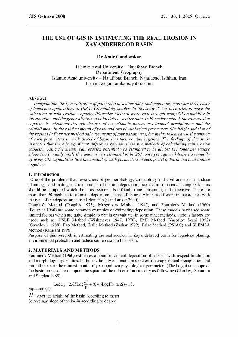
more the rain and the more rain erosion capacity. To compute average annual rain in Zayanderood

Basin, They used average 30 years annual rain of the synoptic, climatology and rain gauge station

inside and around Zayanderood Basin and interpolation was done by Kriging method and then the

map of the isohyets lines was sketched (Figure 1).

50.1 50.2 50.3 50.4 50.5 50.6 50.7

32.4

32.5

32.6

32.7

32.8

32.9

33

33.1

0Km 10Km 20Km

Figure 1: Annual isohyets lines map of Zayanderood Basin

In accordance with this, in Zayanderood Basin the average annual precipitation differs from about 290

mm in North eastern part of the basin to about 1380 mm in South western parts of the basin and the

average precipitation in the basin is about 534 mm.

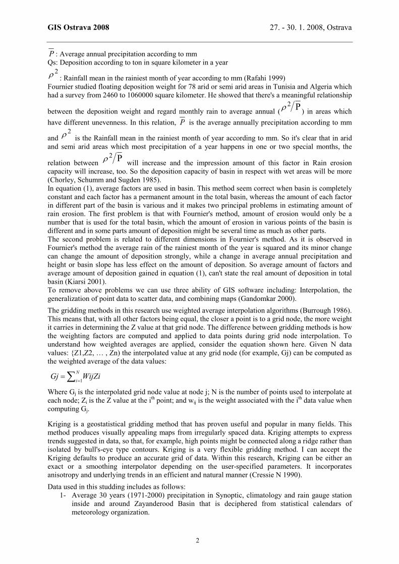
Average 30 years rain in March (the rainiest month) is used to find the interpolation with Kriging

Method and the map relation to monthly isohyets lines in March is sketched (Figure 2).

According to these computations amount of the rain in the rainiest month of the year in the basin a

differs from about 53 mm in North eastern parts of basin to about 320 mm in western parts of basin

and average rain in March in the whole basin is about 105 mm.

GIS Ostrava 2008 27. - 30. 1. 2008, Ostrava

4

50.1 50.2 50.3 50.4 50.5 50.6 50.7

32.4

32.5

32.6

32.7

32.8

32.9

33

33.1

0Km 10Km 20Km

Figure 2: March isohyets lines map of Zayanderood Basin

50.1 50.2 50.3 50.4 50.5 50.6 50.7

32.4

32.5

32.6

32.7

32.8

32.9

33

33.1

0Km 10Km 20Km

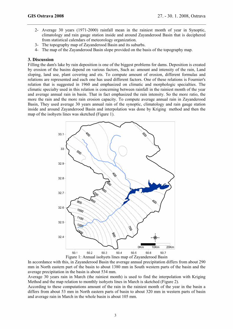
Figure3: Contour map of Zayanderood Basin

GIS Ostrava 2008 27. - 30. 1. 2008, Ostrava

5

To provide information related to contour map of the Zayanderood Basin topography map is used, and

map's data conversed to the numerical data. Then with Kriging Method we found interpolation of the

data and the contour map was sketched (Figure3).

In this basin, the least height is about 2080 meter and the most is about 4040 meter and the area

average height is about 2473 meter.

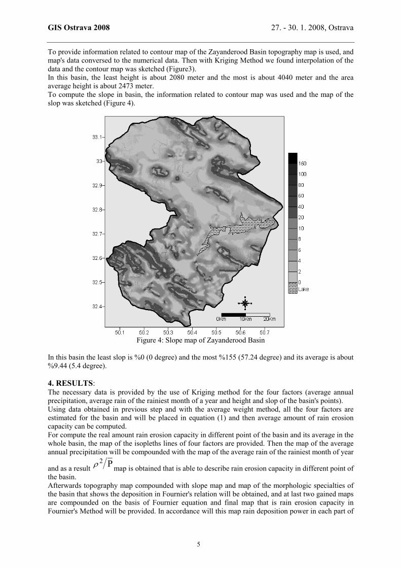
To compute the slope in basin, the information related to contour map was used and the map of the

slop was sketched (Figure 4).

Figure 4: Slope map of Zayanderood Basin

In this basin the least slop is %0 (0 degree) and the most %155 (57.24 degree) and its average is about

%9.44 (5.4 degree).

4. RESULTS: The necessary data is provided by the use of Kriging method for the four factors (average annual

precipitation, average rain of the rainiest month of a year and height and slop of the basin's points).

Using data obtained in previous step and with the average weight method, all the four factors are

estimated for the basin and will be placed in equation (1) and then average amount of rain erosion

capacity can be computed.

For compute the real amount rain erosion capacity in different point of the basin and its average in the

whole basin, the map of the isopleths lines of four factors are provided. Then the map of the average

annual precipitation will be compounded with the map of the average rain of the rainiest month of year

and as a result P2ρ

map is obtained that is able to describe rain erosion capacity in different point of

the basin.

Afterwards topography map compounded with slope map and map of the morphologic specialties of

the basin that shows the deposition in Fournier's relation will be obtained, and at last two gained maps

are compounded on the basis of Fournier equation and final map that is rain erosion capacity in

Fournier's Method will be provided. In accordance will this map rain deposition power in each part of

GIS Ostrava 2008 27. - 30. 1. 2008, Ostrava

6

that basin can be defined and computed its average amount with average weight method for the whole

basin.

After computing the average of all the four factors used in Fournier's equation and by placing their

amount in equation (1) the average rain erosion in Zayanderood Basin was calculated: In this way,

average amount of rain erosion in the basin was estimated about 121 ton/square kilometer in a year.

This amount is average number and in fact the whole basin is supposed constant, while in some parts

the amount of erosion might be several times as much as other parts.

To solve the problem, we used GIS abilities and compounded the map made in previous step in

Fournier's equation and at last a map of the erosion was obtained, so that amount of the rain erosion

capacity in each point was computed separately. Then by average weight, the real amount of the rain

erosion power in the area was computed.

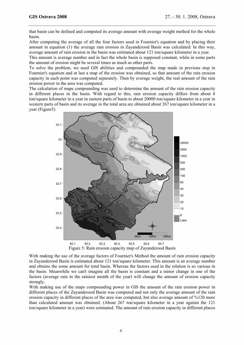
The calculation of maps compounding was used to determine the amount of the rain erosion capacity

in different places in the basin. With regard to this, rain erosion capacity differs from about 8

ton/square kilometer in a year in eastern parts of basin to about 20000 ton/square kilometer in a year in

western parts of basin and its average in the total area are obtained about 267 ton/square kilometer in a

year (Figure5).

50.1 50.2 50.3 50.4 50.5 50.6 50.7

32.4

32.5

32.6

32.7

32.8

32.9

33

33.1

8

10

20

30

40

60

100

200

500

1000

5000

20000

0Km 10Km 20Km

Lake

Figure 5: Rain erosion capacity map of Zayanderood Basin

With making the use of the average factors of Fournier's Method the amount of rain erosion capacity

in Zayanderood Basin is estimated about 121 ton/square kilometer. This amount is an average number

and obtains the some amount for total basin. Whereas the factors used in the relation is so various in

the basin. Meanwhile we can't imagine all the basin is constant and a minor change in one of the

factors (average rain in the rainiest month of the year) will change the amount of erosion capacity

strongly.

With making use of the maps compounding power in GIS the amount of the rain erosion power in

different places of the Zayanderood Basin was computed and not only the average amount of the rain

erosion capacity in different places of the area was computed, but also average amount of %120 more

than calculated amount was obtained. (About 267 ton/square kilometer in a year against the 121

ton/square kilometer in a year) were estimated. The amount of rain erosion capacity in different places

GIS Ostrava 2008 27. - 30. 1. 2008, Ostrava

7

of the Zayanderood Basin was calculated too. So programmers can perform the plans regarded to the

difference in the rain erosion power in different places of the basin.

LITERATURE REFERENCES

Boardman J and Foster I D L and Dearing J A, 1990, Soil erosion on agricultural land, John Wiley and

Sons Co.

Burrough P A, 1986, Principal of Geographical information systems for land resources assessment,

Oxford, Clarendon Press.

Box J E and Meyer L D, 1984, Adjustment of USLE for cropland soils containing coarse fragments,

S.S.S.A Pub, No 13.

Clifford S. Riebe, 2001, Minimal climatic control on erosion rates in the Sierra Nevada, California,

Journal of Geology, Vol 29, P 447-450.

Cressie N 1990, The Origins of Kriging, Mathematical Geology, v. 22, p. 239-252.

David P. Finlayson and David R. Montgomery, 2003, Modeling large-Scale fluvial erosion in

geographic information system, Journal of Geomorphology, Volume 53, Issues 1-2, Pages 147-164.

Deom A, Gouyon R and Berne C, 2005, Rain erosion resistance characterizations: Link between on-

ground experments and in-flight specifications, Wear, Volume 258, Issues 1-4, Pages 545-551.

Douglas I, 1973, Rates of denudation in selected small catchments in Eastern Australia, University of

Hull Occasional Papers in Geography 21.

Fournier M F, 1960, Climate et erosion, Paris, Presses universities de France.

Gandomkar A, 2000, Hydrogeomorphology of upstream Boshar River, Isfahan, P 110 – 120.

Gavrilovic Z, 1988, The use of an empirical method (Erosion potential Method) for calculating

sediment production and transportation in unstudied or torrential streams, International conference on

River regime, Published by John Wiley and Sons, Paper 12, P 411- 422.

Janda R J, 1971, An evaluation of procedures used in computing chemical denudation rates, Bulletin

of the Geological Society of America, Vol 82, P 67 – 80.

Kiarsi F, 2001, Hydrogeomorphology of mean stream Boshar River, Isfahan, P 115 – 130.

Khawlie M, Awad M, Shaban, A, Bou Kheir R and Abdallah C, 2002, Remot sensing for

environmental protection of the eastern Mediterranean rugged mountainous areas, Lebanan, ISPRS

Journal of Photogrammetry and Remot Sensing, Volum 57, Issues 1-2, Pages 13-23

Kenneth G and Jeremy R, 1994, Using monthly precipitation data to estimate the R-factor in the

revised USLE, Journal of Hydrology, Volume 157, Issues 1-4, Pages 287-306.

Langbein W B and Schumm S A, 1958, Yield of sediment in relation to mean annual precipitation,

Transactions of the American Geophysical union, Vol 39, P 1076 – 1084.

Meyer L D, 1981, How rain intensity affects in Terrill erosion, Trans, Am, Soc, Agric, Engnrs 2.

Morgan R P C, 1986, Soil erosion and conservation, Longman scientific and technical, John Wiley

and Sons.

Ramesht M, 1996, Using geomorphology in planning, Isfahan.

Rafahi H, 1999, Soil erosion by water of conservation, Tehran, P 233 – 268.

Rpmero-Diaz A, Alonso-Sarria F and Martinez-Lioris M, 2007, Erosion rates obtained from check-

dam sedimentation (SE Spain). A multi-method comparison, CATENA, Volume 71, Issue 1, Pages

172-178.

Sauerborn P, Klein A, Botschek J and Skowronek A, 1999, Future rainfall erosivity derived from

large-scale climate models – methods and scenarios for a humid region, Geodema, Volume 93, Issues

3-4, Pages 269-276

Stoddart D R, 1969, World erosion and sedimentation, in R J Chorley, Water, Earth and Man, London,

Methuen P 43 – 64.

Wilson L, 1973, Variations in mean annual sediment yield as a function of mean annual precipitation,

American Journal of Science, Vol 273, P 335 – 349.

Wishmeier W H, 1976, Use and misuse of universal soil loss equation, Journal of Soil and Water

conversation Vol 31.