Embed Size (px)
Citation preview
THE MACRO-ECONOMIC IMPACT OF BREXIT:
USING THE CBR MACRO-ECONOMIC MODEL OF THE UK
ECONOMY (UKMOD)
Centre for Business Research, University of Cambridge, Working Paper no. 483
by
Graham Gudgin
CBR, University of Cambridge
Ken Coutts
CBR, University of Cambridge
Neil Gibson
Ulster University Economic Policy Centre
Jordan Buchanan
Ulster University Economic Policy Centre
May 2017
This is a revised version of a working paper first published in December 2016
Abstract. This working paper uses the new CBR macro-economic model of the
UK economy to investigate possible futures following the referendum decision
to leave the EU. The paper briefly explains why we felt the necessity to build a
new model and describes some of its key features. Since Brexit is a unique event
with no precedent it is not possible to do a normal forecast in which a few
assumptions are made about a limited range of exogenous variables. The best that
can be done is to construct scenarios and two are presented here. The difficult
part is to decide what scale of adjustment is needed to reflect the likely realities
of Brexit. Gravity model analysis by HM Treasury of the potential impact of
various outcomes for trade outside the EU is examined and found wanting. The
gravity model approach is replicated and shows that the impact of EU
membership on the level of exports to the EU is much smaller for the UK than
for other EU members. The implication is that the impact of EU membership on
UK trade is much less than suggested by the Treasury
In addition the actual experience of UK export performance is examined for a
long period including both pre- and post- accession years. This augments the
gravity model results in suggesting a more limited impact of EU membership.
While we include a scenario based on Treasury assumptions, a more realistic,
although in our view still pessimistic, scenario assumes a much lower level of the
trade loss than that of the Treasury. The results are presented through comparing
these scenarios with a pre-referendum forecast. In the milder Brexit scenario there
is a minor loss of GDP by 2025 (around 1%) but no loss of per capita GDP, and
also less unemployment but more inflation. In the more severe, Treasury-based
scenario the loss of GDP is nearer 4% (2.5% for per capita GDP), inflation is
higher and the advantage in unemployment less.
JEL Classification: E12; E17; E27; E37; E47; E66; F17
Keywords: Brexit; H M Treasury; macroeconomic policy; fiscal and monetary
policy; macroeconomic forecasts; macroeconomic models.
Acknowledgements We are grateful for comments made on a version of this
paper at a seminar in the St. Catharine’s College series in Cambridge, November
2016.
Further information about the Centre for Business Research can be found at:
www.cbr.cam.ac.uk
1
Introduction
The result of the referendum on membership of the European Union in June 2016
generated a large shock to the UK economy. Even after triggering the formal Article
50 mechanism in March 2017 to begin the process of leaving, the final arrangements
for trade and migration are not yet known. The UK government intends to achieve
an exit from the EU which returns control of migration to the UK, involving leaving
the single market, and removing the UK from the jurisdiction of the European Court
of Justice. The aim is to secure a free trade agreement with the remainder of the EU,
but if this is not feasible then the UK will leave without a formal trade agreement
and rely on WTO rules to govern its trade with both the EU and with the rest of the
world.
The UK was already a semi-detached member of the EU, outside both the Euro
single currency area and the Shengen area of passport-free movement of people, and
as a result the likely impact of leaving the EU will be less of a shock than might
otherwise have been the case. Even so, leaving will involve one of the largest
changes in the institutional arrangements for the UK economy since joining the EU
in 1973. It is not of course the only large shock over this period. The accession of
the Eastern European A10 states between 2004 and 2013 represented a large shock,
albeit one not immediately recognised, in setting up the large-scale immigration
flows in the UK which became one of the two strongest factors behind the ‘leave’
vote in the referendum.
In this paper we use the CBR macro-economic model of the UK economy to estimate
the potential impact of what has come to be known as ‘Brexit’. From the outset we
need to say that no normal forecast is possible. The CBR model is an econometric
model which uses a large set of equations to forecast future trends, each equation
based on data covering the last few decades of UK economic behaviour. Because
this period has been almost wholly one in which the UK has been a member of the
EU, the equations contain little or no direct information about how the UK would
fare outside the EU. Put simply, leaving the EU is a unique event; no country has
ever done this. The best we can do is to construct a series of scenarios based on
assumptions about future trading arrangements, migration controls and about the
2
short-term uncertainties which could affect business investment in the run-up to the
likely leaving date of 2019.
Our estimates of the impact of Brexit will depend partly on the nature of the CBR
model and we will say a little about this. Mostly the estimates will reflect the
assumptions entered into the model. Much was written and said during the
referendum campaign about such assumptions, much of it highly controversial. Most
detailed were the two major reports from H.M. Treasury, one on the long-term
impact and the other on the more immediate consequences of a vote to leave1.
Although the analysis in these Treasury reports was inevitably coloured by the
Government’s stated opposition to leaving the EU, the two reports, together
involving 280 pages of analysis, offered a comprehensive literature review and were
based on best practice in that literature. We thus review the Treasury’s methodology
leading to their conclusion that a complete break with the EU Single Market would
lead to a loss in GDP of 7.2% by 2030. Since the Treasury analysis strangely says
little directly about the UK’s trade record within the EU we also examine this in
detail to see whether this supports the more indirect methods used by the Treasury
in assessing the impact of EU membership on the volume of trade.
The CBR Macro-Economic Model
The main burden of this paper involves assessing what assumptions should be
entered into our CBR macro-economic model and then using these assumptions to
generate forecasts for two scenarios over the period 2017-25. These issues are dealt
with below, but first we describe some of the relevant context of the UK economy
and the way in which the CBR model approaches key issues.
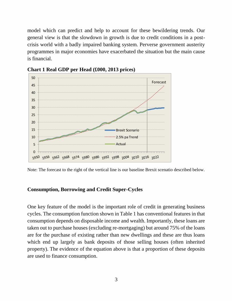
Something has gone badly wrong with economic growth in the UK where a
relatively consistent growth trend of close to 2.5% per annum has comprehensively
broken down (Chart 1). Similarly dramatic breaks of trend can be observed for the
USA and the EU although in the latter case the slowdown began rather earlier in
2000 coinciding with the introduction of the Euro. These breaks of trend are related
to the so-called ‘productivity puzzle’ for which economists have no agreed
explanation. Alongside the failure of existing forecasting models to predict the 2008
economic crisis this break of trend provides another reason for developing a new
3
model which can predict and help to account for these bewildering trends. Our
general view is that the slowdown in growth is due to credit conditions in a post-
crisis world with a badly impaired banking system. Perverse government austerity
programmes in major economies have exacerbated the situation but the main cause
is financial.
Chart 1 Real GDP per Head (£000, 2013 prices)
Note: The forecast to the right of the vertical line is our baseline Brexit scenatio described below.
Consumption, Borrowing and Credit Super-Cycles
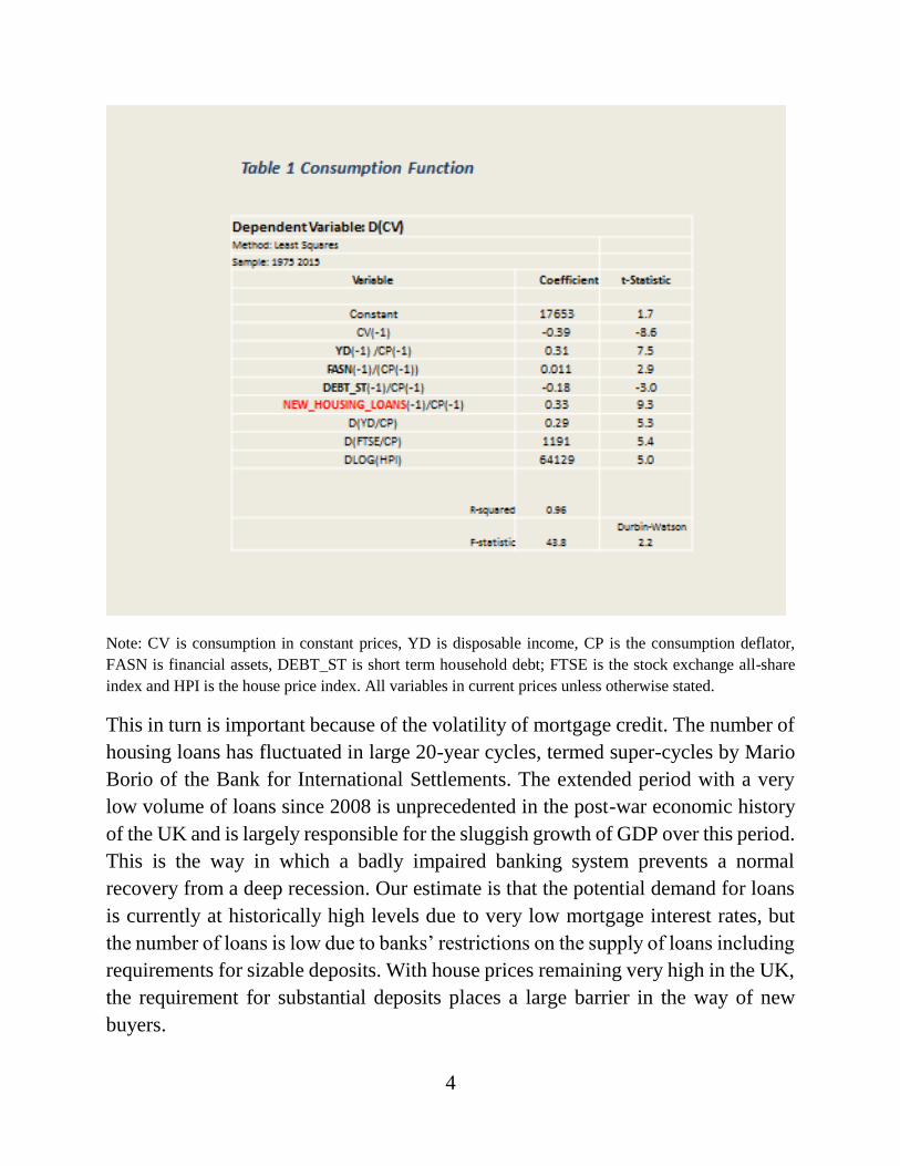
One key feature of the model is the important role of credit in generating business
cycles. The consumption function shown in Table 1 has conventional features in that
consumption depends on disposable income and wealth. Importantly, these loans are
taken out to purchase houses (excluding re-mortgaging) but around 75% of the loans
are for the purchase of existing rather than new dwellings and these are thus loans
which end up largely as bank deposits of those selling houses (often inherited
property). The evidence of the equation above is that a proportion of these deposits
are used to finance consumption.
0
5
10
15
20
25
30
35
40
45
50
Brexit Scenario
2.5% pa Trend
Actual
Forecast
4
Note: CV is consumption in constant prices, YD is disposable income, CP is the consumption deflator,
FASN is financial assets, DEBT_ST is short term household debt; FTSE is the stock exchange all-share
index and HPI is the house price index. All variables in current prices unless otherwise stated.
This in turn is important because of the volatility of mortgage credit. The number of
housing loans has fluctuated in large 20-year cycles, termed super-cycles by Mario
Borio of the Bank for International Settlements. The extended period with a very
low volume of loans since 2008 is unprecedented in the post-war economic history
of the UK and is largely responsible for the sluggish growth of GDP over this period.
This is the way in which a badly impaired banking system prevents a normal
recovery from a deep recession. Our estimate is that the potential demand for loans
is currently at historically high levels due to very low mortgage interest rates, but
the number of loans is low due to banks’ restrictions on the supply of loans including
requirements for sizable deposits. With house prices remaining very high in the UK,
the requirement for substantial deposits places a large barrier in the way of new
buyers.
5
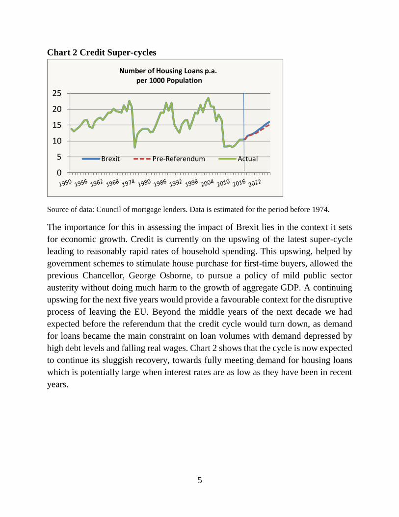
Chart 2 Credit Super-cycles
0
5
10
15
20
25
Number of Housing Loans p.a.per 1000 Population
Brexit Pre-Referendum Actual
Source of data: Council of mortgage lenders. Data is estimated for the period before 1974.
The importance for this in assessing the impact of Brexit lies in the context it sets
for economic growth. Credit is currently on the upswing of the latest super-cycle
leading to reasonably rapid rates of household spending. This upswing, helped by
government schemes to stimulate house purchase for first-time buyers, allowed the
previous Chancellor, George Osborne, to pursue a policy of mild public sector
austerity without doing much harm to the growth of aggregate GDP. A continuing
upswing for the next five years would provide a favourable context for the disruptive
process of leaving the EU. Beyond the middle years of the next decade we had
expected before the referendum that the credit cycle would turn down, as demand
for loans became the main constraint on loan volumes with demand depressed by
high debt levels and falling real wages. Chart 2 shows that the cycle is now expected
to continue its sluggish recovery, towards fully meeting demand for housing loans
which is potentially large when interest rates are as low as they have been in recent
years.
6
Assumptions on Brexit
The difficulty in generating any forecast for the future of the UK economy is in
knowing what to assume about both future trade arrangements and the short-term
impact of uncertainty about these arrangements. As we have stated, the best that is
possible is to generate scenarios based on assumptions about these things. This is
not to say that there is little on which to base assumptions. A plethora of reports
were produced during the referendum campaign to assess what the impact might be
of a vote to leave the EU and, several months on from the referendum, some
consequences have also begun to emerge.
Short-term Impact of Brexit
These reports published during the referendum campaign generally produced
separate estimates for both the short-term impact of uncertainty and the long-term
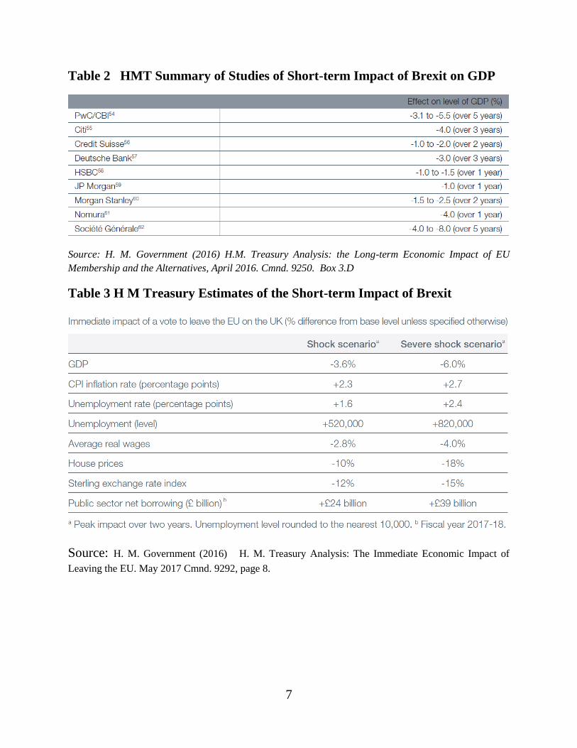
impact of changed trading arrangements. A summary of short-term impacts from
non-government sources is shown in table 2. The government’s own estimates are
shown in Table 3. The estimates vary depending on what is assumed about the nature
of the likely eventual relationship sought with the EU. In general the largest
estimates of losses of GDP stem from an expectation that the UK will leave the
single market and fall back on WTO rules. Something of a consensus emerges from
these studies with an expectation that uncertainty will reduce GDP (relative to a pre-
referendum baseline) by around 1% after one year, 2-4% after 2 years, 3-4% after
three years and 4-6% after 5 years. The Treasury’s estimates are at the high end of
this spectrum of views with a view that GDP would be reduced by between 3.5%
and 6%.
7
Table 2 HMT Summary of Studies of Short-term Impact of Brexit on GDP
Source: H. M. Government (2016) H.M. Treasury Analysis: the Long-term Economic Impact of EU
Membership and the Alternatives, April 2016. Cmnd. 9250. Box 3.D
Table 3 H M Treasury Estimates of the Short-term Impact of Brexit
Source: H. M. Government (2016) H. M. Treasury Analysis: The Immediate Economic Impact of
Leaving the EU. May 2017 Cmnd. 9292, page 8.
8
The Treasury summarised its own view in the following words, “The analysis shows
that the economy would fall into recession with four quarters of negative growth.
After two years, GDP would be around 3.6% lower…. the fall in the value of the
pound would be around 12%, and unemployment would increase by around
500,000, with all regions experiencing a rise in the number of people out of work.
The exchange-rate-driven increase in the price of imports would lead to a material
increase in prices, with the CPI inflation rate higher by 2.3 percentage points after
a year”. 2
The mechanism underlying the Treasury assessment is that firms and households
would begin adjusting to the expected new relationship with the EU, and business
investment would be damaged by uncertainty. Financial markets would react
immediately with a 10-14% fall in the sterling exchange rate. Consumer spending
would be reduced because higher inflation occasioned by a lower exchange rate
would lead to lower real wages. Exports would be higher and imports lower but the
overall impact would be sharply negative. Some econometric work was done to
assess the relationship between measures of uncertainty and key macro-economic
variables. However the actual judgement on uncertainty impacts is arbitrary with the
assumption of a 1 to 1.5 standard deviation rise in uncertainty. A similar assumption
is used to obtain the financial markets effect resulting in a 1 -2 percentage point rise
in market interest rates and equity risk premia.
Writing almost a year after the referendum result, only one of the Treasury’s
expectations has been clearly realized. This is the fall in the value of sterling. A 12%
fall in the effective exchange rate matches the HMT ‘severe shock’ scenario. There
was however little movement on interest rates, even after the US Presidential
election result in November 2016 when anticipated higher infrastructure spending
and higher expected inflation quickly drove bond yields upwards. The UK Treasury
expectation that equity risk premia would rise, leading to lower equity prices, has
thus proved wrong. The sterling depreciation instead led to higher UK equity prices
as corporate earnings from abroad became worth more in sterling. Preliminary data
also suggest little or no fall in consumption, house prices or house building. GDP in
the third and fourth quarters of 2016 was well above Treasury expectations, although
slow growth in the first quarter of 2017 may indicate the start of a period of slower
growth.
9
Our own expectation has been that there would be little direct impact of Brexit on
consumer spending or investment in housing. Since, as we argue below, the long-
term impact of Brexit is expected to be well below Treasury estimates, even if the
UK ends up with no free trade agreement or other privileged access to the EU Single
Market, our expectation of any transitional losses to investment would be relatively
small. Uncertainty effects on company investment are harder to assess. It seems
reasonable to expect that at least some domestic firms will delay investment until
they are clearer about future trade arrangements; foreign direct investment will be
reduced partly for the same reasons and also because some firms wish to locate
within the EU. The initial evidence to date has been mixed. Several strategically
important firms have announced major investments. Others, particularly in financial
services are said to be at least exploring the possibility of relocating some activities
into the continuing EU. These announcements have no doubt influenced the OBR in
the March 2017 forecasts released in conjunction with the Chancellor’s Spring
Budget. Their forecast of GDP growth of 2.0% in 2017 is a long way from the
Treasury’s four quarters of negative growth3.
We have made two arbitrary assumptions on short-term impacts to drive our Brexit
scenarios. We propose two scenarios. A severe scenario broadly matches Treasury
expectations even though we view these as unrealistic. A mild scenario assumes a
significant but milder reduction in business investment. In the mild scenario net new
business investment is arbitrarily reduced in 2017 by close to 3% below the pre-
referendum baseline, after which uncertainty reduces and some recovery of
investment occurs. In the severe scenario the reduction in business investment is
closer to 30%. The sterling effective exchange rate is assumed to depreciate
immediately by 10%, although some of the depreciation into 2017 was already
projected in our pre-referendum baseline forecast. The impact on consumer
spending, household investment and exports and imports are all indirect
consequences of the above assumptions without any more direct impacts.
10
Long-term Impact of Brexit
It is widely accepted that the long-term impact of Brexit depends on the trade
arrangements agreed for the UK after leaving the EU. Several forecasters have made
separate estimates for the UK joining the European Economic Area (EEA),
negotiating a new free-trade agreement with the EU, or most drastically having no
agreement and falling back on World Trade Organisation (WTO) rules. In this paper
we focus on the last of these three as the putative worst-case scenario. Other
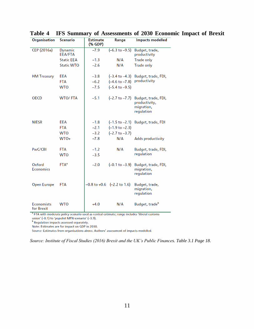
scenarios should not be as bad for the UK. The Institute for Fiscal studies (IFS)
usefully summarised the range of estimates for fourteen years after the referendum
(Table 4). Several major forecasters (Treasury, OECD, NIESR and the LSE’s Centre
For Economic Policy (CEP) broadly agree that leaving the single market and falling
back on WTO rules would lead to GDP being more than 7% lower by 2030 than it
would otherwise have been. PwC, Oxford Economics and Open Europe have lower
impacts for the scenarios they consider, but the main reason seems to be that they
exclude the productivity effects included in the Treasury, OECD, NIESR and CES
studies. The one clear outlier is that of the Economists for Brexit led by the free-
market economists Patrick Minford and Gerard Lyons. The main reason for the
positive impact of Brexit in their study appears to be their assumption that all exports
and imports behave like oil and other commodities. Commodities can always be sold
in world markets at prevailing world prices, and hence being shut out of any
particular market makes little difference. This seems to us an assumption which,
although true for some exports and more imports, is not representative of most
exports.
11
Table 4 IFS Summary of Assessments of 2030 Economic Impact of Brexit
Source: Institute of Fiscal Studies (2016) Brexit and the UK’s Public Finances. Table 3.1 Page 18.
12
How Does the Treasury estimate its Long-term Impact?
In this paper we focus on the Treasury’s assessment of the long-term impact of
Brexit as a representative example. The Treasury examines three possible cases
(EEA, FTA and WTO rules) and we take only the last of these as an example of a
worst-case scenario. The Treasury report4 made estimates of three macro-economic
variables and then inserted these estimates into the NIESR’s NiGEM model to
calculate overall impacts on GDP and GDP per head. The three variables are:
Trade (exports and imports)
Foreign Direct Investment (FDI)
Productivity (GDP per head)
The Treasury’s estimates for WTO rules
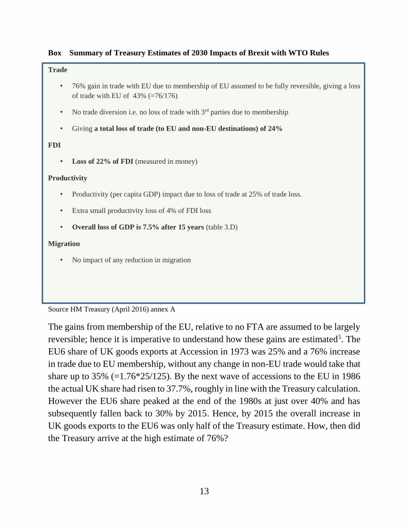
The Treasury’s estimates are summarised in the Box below. These estimates are for
a case in which the UK leaves the EU without joining the European Economic Area
or concluding a new free-trade agreement. The estimated loss of trade with the EU
in this option is very large at 43%, and is based on coefficients from econometric
work which the Treasury regards as being in line with academic studies. The same
work leads the Treasury to conclude that these losses would not be offset by any
gains in trade with non-EU countries.
13
Box Summary of Treasury Estimates of 2030 Impacts of Brexit with WTO Rules
Trade
• 76% gain in trade with EU due to membership of EU assumed to be fully reversible, giving a loss
of trade with EU of 43% (=76/176)
• No trade diversion i.e. no loss of trade with 3rd parties due to membership
• Giving a total loss of trade (to EU and non-EU destinations) of 24%
FDI
• Loss of 22% of FDI (measured in money)
Productivity
• Productivity (per capita GDP) impact due to loss of trade at 25% of trade loss.
• Extra small productivity loss of 4% of FDI loss
• Overall loss of GDP is 7.5% after 15 years (table 3.D)
Migration
• No impact of any reduction in migration
Source HM Treasury (April 2016) annex A
The gains from membership of the EU, relative to no FTA are assumed to be largely
reversible; hence it is imperative to understand how these gains are estimated5. The
EU6 share of UK goods exports at Accession in 1973 was 25% and a 76% increase
in trade due to EU membership, without any change in non-EU trade would take that
share up to 35% (=1.76*25/125). By the next wave of accessions to the EU in 1986
the actual UK share had risen to 37.7%, roughly in line with the Treasury calculation.
However the EU6 share peaked at the end of the 1980s at just over 40% and has
subsequently fallen back to 30% by 2015. Hence, by 2015 the overall increase in
UK goods exports to the EU6 was only half of the Treasury estimate. How, then did
the Treasury arrive at the high estimate of 76%?
14
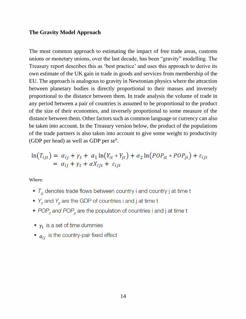
The Gravity Model Approach
The most common approach to estimating the impact of free trade areas, customs
unions or monetary unions, over the last decade, has been “gravity” modelling. The
Treasury report describes this as ‘best practice’ and uses this approach to derive its
own estimate of the UK gain in trade in goods and services from membership of the
EU. The approach is analogous to gravity in Newtonian physics where the attraction
between planetary bodies is directly proportional to their masses and inversely
proportional to the distance between them. In trade analysis the volume of trade in
any period between a pair of countries is assumed to be proportional to the product
of the size of their economies, and inversely proportional to some measure of the
distance between them. Other factors such as common language or currency can also
be taken into account. In the Treasury version below, the product of the populations
of the trade partners is also taken into account to give some weight to productivity
(GDP per head) as well as GDP per se6.
Where:
15
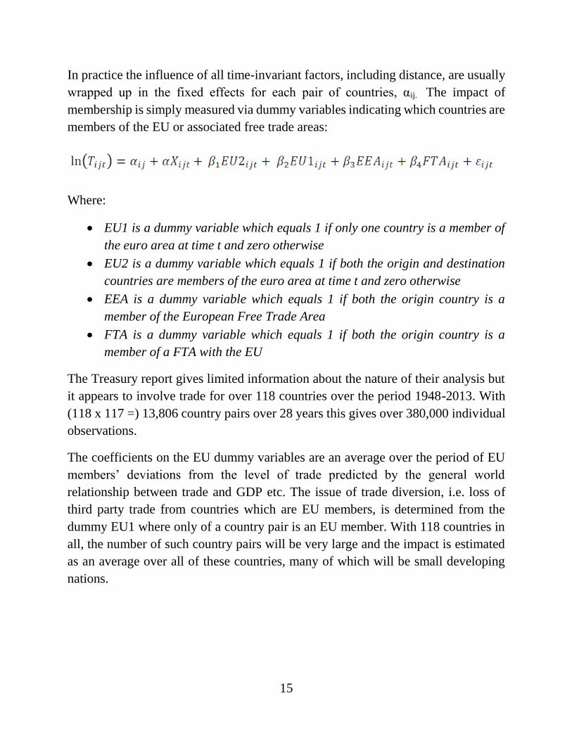
In practice the influence of all time-invariant factors, including distance, are usually
wrapped up in the fixed effects for each pair of countries, αij. The impact of
membership is simply measured via dummy variables indicating which countries are
members of the EU or associated free trade areas:
Where:
EU1 is a dummy variable which equals 1 if only one country is a member of
the euro area at time t and zero otherwise
EU2 is a dummy variable which equals 1 if both the origin and destination
countries are members of the euro area at time t and zero otherwise
EEA is a dummy variable which equals 1 if both the origin country is a
member of the European Free Trade Area
FTA is a dummy variable which equals 1 if both the origin country is a
member of a FTA with the EU
The Treasury report gives limited information about the nature of their analysis but
it appears to involve trade for over 118 countries over the period 1948-2013. With
(118 x 117 =) 13,806 country pairs over 28 years this gives over 380,000 individual
observations.
The coefficients on the EU dummy variables are an average over the period of EU
members’ deviations from the level of trade predicted by the general world
relationship between trade and GDP etc. The issue of trade diversion, i.e. loss of
third party trade from countries which are EU members, is determined from the
dummy EU1 where only of a country pair is an EU member. With 118 countries in
all, the number of such country pairs will be very large and the impact is estimated
as an average over all of these countries, many of which will be small developing
nations.
16
The Treasury is thus relying on averages across a range of EU member states at
different dates, rather than on the direct experience of the UK itself. Indeed, the
Treasury analysis provides virtually no information directly about UK trade with the
EU. We will return to this issue below, but will first complete a description of the
Treasury approach to estimating the overall impact of Brexit.
Service sector trade
A similar approach is used to estimate the impact of EU membership on trade in
services. Once again the data includes a large range of countries over the period
1981-2009. Once again the method finds a positive impact of EU membership,
albeit smaller than for goods, and no evidence of trade diversion.
The Impact on FDI
The Treasury again uses a gravity model to assess the extent to which EU
membership increases the flow of foreign direct investment between country pairs.
The data in this case covers 40 countries over the period 2000-14. Although the
Treasury does not say so, the data is in the form of financial flows. It thus includes
financing flows and mergers and acquisitions alongside physical investment projects
such as new green-field sites or extensions to existing sites. The Treasury does admit
that the data is troublesome due to profit shifting for tax reasons. In fact the data can
be very difficult, with annual FDI inflows into Luxemburg in recent years averaging
320% of GDP and flows into Ireland and the Netherlands averaging 25% of GDP.
Our own estimates for the UK are that under a quarter of FDI flows measured in
money terms relate to new physical investment projects7. The issue then is: even if
EU membership increases FDI flows in money it is difficult to assess what impact
this will have on an individual economy. The impact of new physical investment is
likely to be very different from acquisitions or profit-shifting.
The estimation period used in this analysis i.e. 2000-14 means that the results are
dominated by countries which joined the EU in these years. These were of course
17
largely Eastern-European post-Soviet bloc countries with very low labour costs. The
impact of EU membership was generally very large, as restrictions on inward
investment from the EU were removed and EU-based companies were able to take
advantage of the low cost of labour. The analysis estimates that EU membership
increased FDI flows by 22% with no diversion from other countries, but it is difficult
to know what this implies for physical FDI flows into the UK and hence for UK
economic development.
Impact on Productivity
The Treasury Report summarises a few academic reports linking expansion in trade
and FDI to increases in economy-wide or firm productivity. Some of the trade
studies are based on a gravity model methodology. Once again the relationships
emerging from these studies are based on the experience of up to 200 countries. Most
of these countries are once again necessarily small emerging economies. In some
cases, trade increases as economies emerge from behind high tariff walls allowing
multi-national companies to operate. In these circumstances it is unsurprising that
aggregate productivity rises, but it is not obvious that these results can be applied to
a well-developed open economy like the UK leaving a single market and customs
union with generally low tariffs.
An average elasticity of 0.25 is drawn by the Treasury from this literature. Even if
this were applicable, any impact depends on the size of the trade losses based on
gravity model studies which, in our view, are unreliable. Two established
practitioners of this approach recently published a ’mea culpa’ in which they
discovered that their earlier results were extremely sensitive to equation
specification. They concluded that it is “currently beyond our ability to estimate the
effect of currency unions on trade with much confidence”8.This paper referred to
trade and currency unions but it seems likely that the conclusions apply to similar
studies of trade and customs unions.
The Treasury also cites a number of firm-level studies. It is well known that foreign-
owned firms generally have higher productivity than domestic companies -much of
this is because the former are more likely to be exposed to greater competition and
18
to be involved in international trade and foreign direct investment. The ‘most
comprehensive of these studies in the view of the Treasury is the study by Melitz
and Trifler showing that productivity in Canadian manufacturing grew by 14% from
1988-96 following Canada’s joining the US-Canada FTA in 1989 and the full
NAFTA in 1993. What the Treasury did not say was that part of the effect was due
to an 18% loss of jobs in low productivity plants in Canada. Nor did they apparently
know that the impact on the Canadian economy as a whole was entirely the opposite.
Per capita GDP fell sharply in 1990 and has never regained the 2.5% per annum
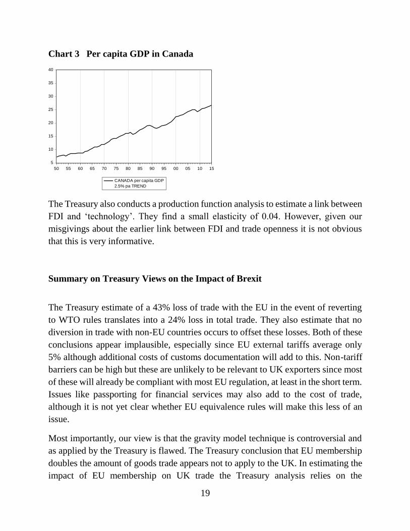
growth trend established over the previous four decades and more (Chart 3). What
seems to have happened is that opening Canada to greater competition raised
productivity in a range of surviving manufacturing firms but displaced a significant
amount of labour in low productivity sectors. Importantly, this labour was never re-
employed at pre-NAFTA levels of productivity. This may be a general process since
most countries joining the EU at various dates between 1970 and 1996 had a similar
experience. This includes the UK joining in 1973.
19
Chart 3 Per capita GDP in Canada
The Treasury also conducts a production function analysis to estimate a link between
FDI and ‘technology’. They find a small elasticity of 0.04. However, given our
misgivings about the earlier link between FDI and trade openness it is not obvious
that this is very informative.
Summary on Treasury Views on the Impact of Brexit
The Treasury estimate of a 43% loss of trade with the EU in the event of reverting
to WTO rules translates into a 24% loss in total trade. They also estimate that no
diversion in trade with non-EU countries occurs to offset these losses. Both of these
conclusions appear implausible, especially since EU external tariffs average only
5% although additional costs of customs documentation will add to this. Non-tariff
barriers can be high but these are unlikely to be relevant to UK exporters since most
of these will already be compliant with most EU regulation, at least in the short term.
Issues like passporting for financial services may also add to the cost of trade,
although it is not yet clear whether EU equivalence rules will make this less of an
issue.
Most importantly, our view is that the gravity model technique is controversial and
as applied by the Treasury is flawed. The Treasury conclusion that EU membership
doubles the amount of goods trade appears not to apply to the UK. In estimating the
impact of EU membership on UK trade the Treasury analysis relies on the
5
10
15
20
25
30
35
40
50 55 60 65 70 75 80 85 90 95 00 05 10 15
CANADA per capita GDP
2.5% pa TREND
20
coefficients of a dummy variable for EU membership. In principle this is reasonable,
but the value of the coefficient obviously depends on the underlying equation. In the
Treasury analysis this equation is estimated over a very large number of countries
most of which are involved in minimal levels of trade with the UK. The estimate is
also an average across EU members and is estimated over the long period spanning
almost three decades. In the annex to this paper we estimate a gravity model for
goods trade. This analysis generates a smaller coefficient for EU membership than
does the Treasury analysis and a much smaller impact for the UK alone (see annex
B).
The Treasury approach also assumes that the EU coefficient captures the beneficial
impact of the Single Market on trade between EU members, but in our view this
cannot be the entire impact. A major additional factor is the growth of demand for
imports within the EU compared with elsewhere. The fact that the EU, and especially
Eurozone, economies have grown so slowly over recent decades has meant that
exports to EU countries have grown less rapidly than exports to other destinations9.
This will affect all exporters but especially those which undertake most trade with
EU countries, and hence mainly the EU countries themselves. Since gravity models
estimate the amount of extra trade occurring between EU members, after allowing
for the size of the economies, the measure does not take account of any slower growth
in the sizes of EU economies relative to non-EU economies. Even if there are
persistent benefits from EU membership due to an absence of tariffs and border
controls, and to uniform regulations, there will be offsetting disadvantages from
slow growth. Our estimate in Annex B of the impact of EU membership on UK
exports is relatively stable over time, but as we show in the next section actual UK
exports to the EU have grown over the last decade much more slowly than UK
exports to non-EU destinations.
The Treasury has used an impact for membership of the Single Market which is
average over all member states. The evidence of our analysis indicates that the UK
experience is very different from the other member states. It turns out that UK
exports to EU partners are much lower than predicted by our equation with the single
exception of exports to Ireland. This may also be the case in the Treasury analysis
but their report makes no comment on this, even though an earlier Treasury paper
showed clearly that the impact of EU membership on goods trade was much smaller
than the average impact across all EU members10.
21
Since the loss of trade turns out to be much lower in our analysis than in that of the
Treasury, the Treasury’s assumption that a loss of trade will reduce productivity
becomes less important. In any case it is not obvious that a productivity link of this
magnitude based on evidence dominated by emerging economies is appropriate for
the Brexit situation. Nor is the evidence cited on FDI impressive, although there is
likely to be some loss of physical FDI.
Another issue ignored in the Treasury analysis is the importance of exchange rates.
The 12% depreciation of sterling that occurred immediately after the Referendum
will do much to offset EU tariffs on EU exports. Our estimate is, for instance, that a
15% depreciation of sterling relative to the euro is sufficient to offset the impact of
a 10% EU external tariff on motor vehicles, including the higher costs of
intermediate imports to this sector. For most engineering firms, tariffs of close to 2%
are small in relation to a sterling depreciation of this magnitude.
Our preferred gravity model equation agrees with the Treasury in indicating that
there is no evidence that membership of the EU has led to reduced exports to non-
EU markets. However, this does not mean in our view that leaving the EU cannot
result in increased exports to non-EU markets. We do not go as far as the
‘Economists for Brexit’ in assuming that all exports lost in EU markets can be sold
in non-EU markets11, but it defies logic to move to the opposite extreme and accept
the Treasury estimate that no trade will be diverted. Some UK exports (e.g. milk
powder) are commodities that can be sold on world markets as the Economists for
Brexit suggest. For other exports it may take longer, in some cases much longer, to
build additional export sales.
In summary, we regard much of the Treasury evidence on the likely impact of Brexit
on trade, FDI and productivity to be flawed and not directly relevant to the likely
impact on UK trade from leaving the EU. Our attempt to replicate the gravity model
analysis, reported in annex B, generated very different conclusions to those of the
Treasury. It was a serious weakness of the Treasury report that almost no evidence
of the record of UK trade with the EU was included in the analysis. Before outlining
this analysis we examine the direct evidence on UK trade.
Direct Evidence on UK Exports to the EU
22
A different approach to analysing the impact of the UK joining the EU, to get a sense
of what might happen when the UK leaves, is to examine time series data. This
approach compares the pre-accession trends in economic behaviour with post-
accession behaviour. Two variables are of key interest. The first is trade, and we will
examine the EU share of UK exports of goods and services. Instead of looking at the
EU membership at any particular date, we examine a constant set of the current 28
members throughout a period from 1950-2015. Second is productivity. If
membership of the EU is beneficial for productivity, this should show up in the UK’s
productivity record. The difficulty comes in allowing for factors other than EU
membership, especially since the UK’s accession date of 1973 was in many ways a
turning point in post-war economic history, especially in Western Europe.
Data Sources
For data on trade we have used the IMF’s Direction of Trade (DOT) series of annual
goods exports by country from 194812. This provides data for our 1950-2015 period
for all of those current member states that have been independent states throughout
the period. Data is thus missing prior to 1990 for the Baltic States, formerly part of
the Soviet Union and Slovenia and Croatia which were part of the former
Yugoslavia. Even without these five states, the data covers 98% of the exports of the
current EU. However for completeness we have estimated UK exports to these five
states for the period prior to 199013.
ONS data on total UK exports of goods and services is available back to 1950. The
IMF DOT data provides data for exports to the EU28 but only for goods. For
services, ONS provides data only from 1999. For earlier years we have assumed that
the EU28 share of UK services exports expanded at the same rate as the share for
goods. The sum of exports of goods and services at current prices is deflated by the
same UK export price deflator whether these exports are to the EU or to other
countries.
23
Productivity is measured as per capita GDP. Data for GDP and population has been
obtained for the EU28 countries from the Conference Board database. GDP is
measured in $1990 at purchasing power parity. Data is converted into sterling using
the average dollar-sterling exchange rate for each year. Missing data for the Baltic
and former Yugoslav States prior to 1990 is estimated in the same way as for trade.
Trends in UK Exports to the EU28
We examine exports to all current EU member states from 1950 to 2015 irrespective
of whether the states were EU members at any particular date, or even whether they
were independent states. This avoids the problem of an EU membership which
changes over time. If membership of the EU promotes trade then we might expect
to see growing exports to the EU28 not only after the UK joined in 1973, but also as
other countries joined in subsequent years and as countries left the Soviet orbit after
the fall of the Iron Curtain in 1989.
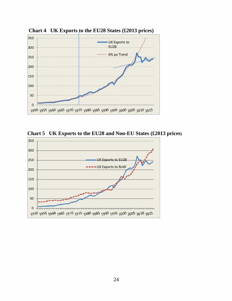
Total exports to the EU28 countries grew surprisingly rapidly through most of the
post-war period (Chart 4). The 6% per annum pre-accession growth trend was
sustained right up until the end of the 20th century, despite the sharp slowdown in
the growth of the European economies14. UK exports to the rest of the world grew
more slowly than exports to the EU28 in the pre-accession period at just over 3%
per annum or around half the rate of exports to the EU28 (Chart 5). This reflected
the more rapid growth of the European economies recovering from the enormous
damage of World War II and catching up with the USA representing the best practice
frontier for technological efficiency. The growth of UK exports to non-EU28
countries clearly slowed down after UK accession in contradiction to the Treasury
finding that no trade diversion took place15. From the millennium, UK exports to
non-EU countries have grown rapidly, and much more rapidly than to the EU. It is
a little-known fact that Commonwealth markets have grown faster than EU markets
since the UK’s historic switch from the former to the latter in 197316.
24
Chart 4 UK Exports to the EU28 States (£2013 prices)
Chart 5 UK Exports to the EU28 and Non-EU States (£2013 prices)
0
50
100
150
200
250
300
350UK Exports toEU28
6% pa Trend
0
50
100
150
200
250
300
350
UK Exports to EU28
UK Exports to RoW
25
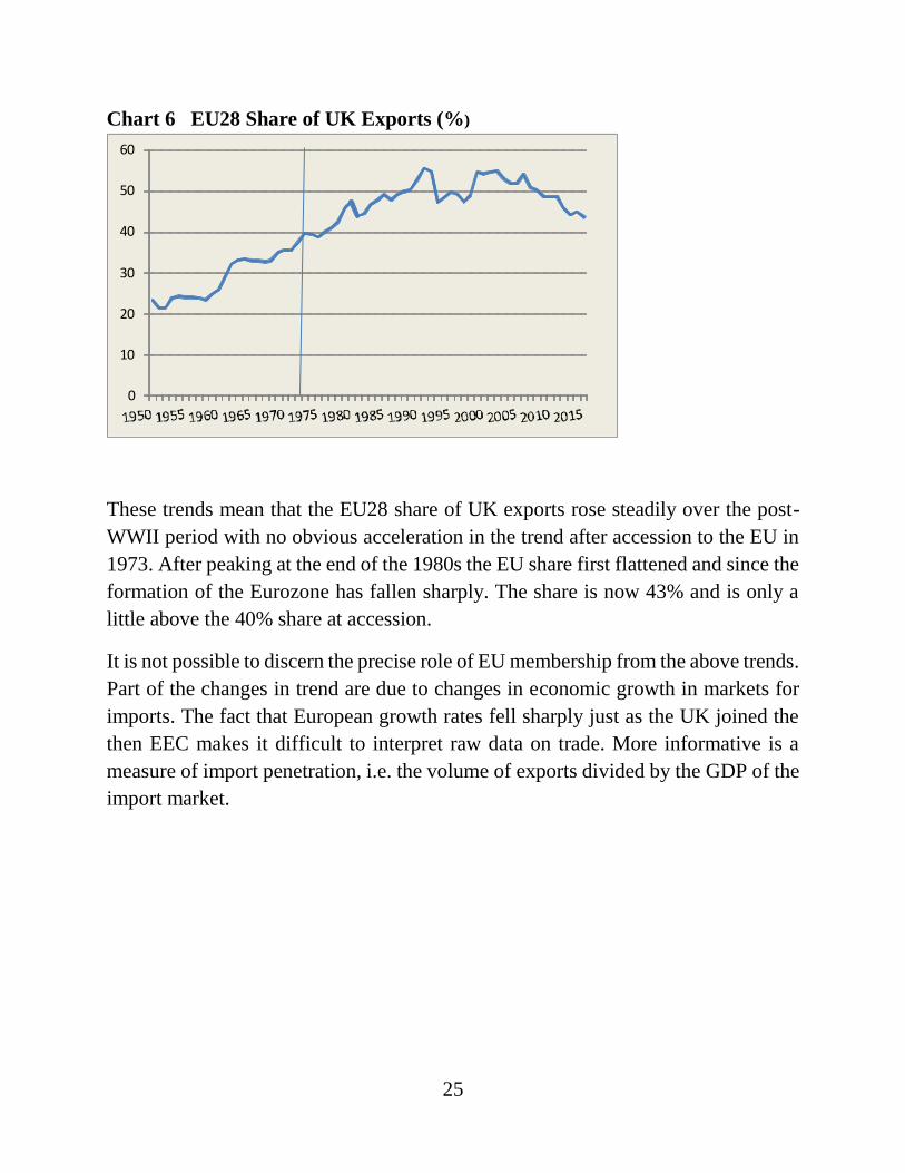
Chart 6 EU28 Share of UK Exports (%)
These trends mean that the EU28 share of UK exports rose steadily over the post-
WWII period with no obvious acceleration in the trend after accession to the EU in
1973. After peaking at the end of the 1980s the EU share first flattened and since the
formation of the Eurozone has fallen sharply. The share is now 43% and is only a
little above the 40% share at accession.
It is not possible to discern the precise role of EU membership from the above trends.
Part of the changes in trend are due to changes in economic growth in markets for
imports. The fact that European growth rates fell sharply just as the UK joined the
then EEC makes it difficult to interpret raw data on trade. More informative is a
measure of import penetration, i.e. the volume of exports divided by the GDP of the
import market.
0
10
20
30
40
50
60
26
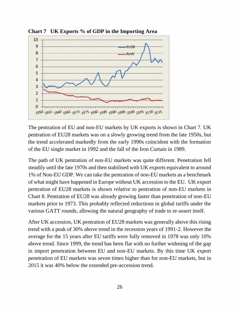
Chart 7 UK Exports % of GDP in the Importing Area
The pentration of EU and non-EU markets by UK exports is shown in Chart 7. UK
pentration of EU28 markets was on a slowly growing trend from the late 1950s, but
the trend accelerated markedly from the early 1990s coincident with the formation
of the EU single market in 1992 and the fall of the Iron Curtain in 1989.
The path of UK pentration of non-EU markets was quite different. Penetration fell
steadily until the late 1970s and then stabilised with UK exports equivalent to around
1% of Non-EU GDP. We can take the pentration of non-EU markets as a benchmark
of what might have happened in Europe without UK accession to the EU. UK export
pentration of EU28 markets is shown relative to pentration of non-EU markets in
Chart 8. Pentration of EU28 was already growing faster than penetration of non-EU
markets prior to 1973. This probably reflected reductions in global tariffs under the
various GATT rounds, allowing the natural geography of trade to re-assert itself.
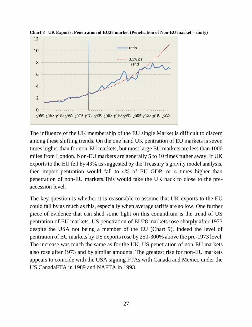
After UK accession, UK pentration of EU28 markets was generally above this rising
trend with a peak of 30% above trend in the recession years of 1991-2. However the
average for the 15 years after EU tariffs were fully removed in 1978 was only 10%
above trend. Since 1999, the trend has been flat with no further widening of the gap
in import penetration between EU and non-EU markets. By this time UK export
penetration of EU markets was seven times higher than for non-EU markets, but in
2015 it was 40% below the extended pre-accession trend.
0
1
2
3
4
5
6
7
8
9
10
EU28
RoW
27
Chart 8 UK Exports: Penetration of EU28 market (Penetration of Non-EU market = unity)
The influence of the UK membership of the EU single Market is difficult to discern
among these shifting trends. On the one hand UK pentration of EU markets is seven
times higher than for non-EU markets, but most large EU markets are less than 1000
miles from London. Non-EU markets are generally 5 to 10 times futher away. If UK
exports to the EU fell by 43% as suggested by the Treasury’s gravity model analysis,
then import pentration would fall to 4% of EU GDP, or 4 times higher than
penetration of non-EU markets.This would take the UK back to close to the pre-
accession level.
The key question is whether it is reasonable to assume that UK exports to the EU
could fall by as much as this, especially when average tariffs are so low. One further
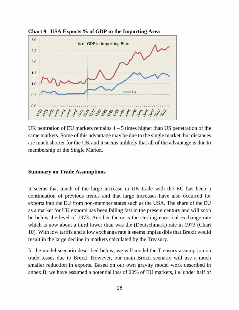
piece of evidence that can shed some light on this conundrum is the trend of US
pentration of EU markets. US penetration of EU28 markets rose sharply after 1973
despite the USA not being a member of the EU (Chart 9). Indeed the level of
pentration of EU markets by US exports rose by 250-300% above the pre-1973 level.
The increase was much the same as for the UK. US penetration of non-EU markets
also rose after 1973 and by similar amounts. The greatest rise for non-EU markets
appears to coincide with the USA signing FTAs with Canada and Mexico under the
US CanadaFTA in 1989 and NAFTA in 1993.
0
2
4
6
8
10
12
ratio
3.5% paTrend
28
Chart 9 USA Exports % of GDP in the Importing Area
0.0
0.5
1.0
1.5
2.0
2.5
3.0% of GDP in Importing Bloc
EU
UK pentration of EU markets remains 4 – 5 times higher than US penetration of the
same markets. Some of this advantage may be due to the single market, but distances
are much shorter for the UK and it seems unlikely that all of the advantage is due to
membership of the Single Market.
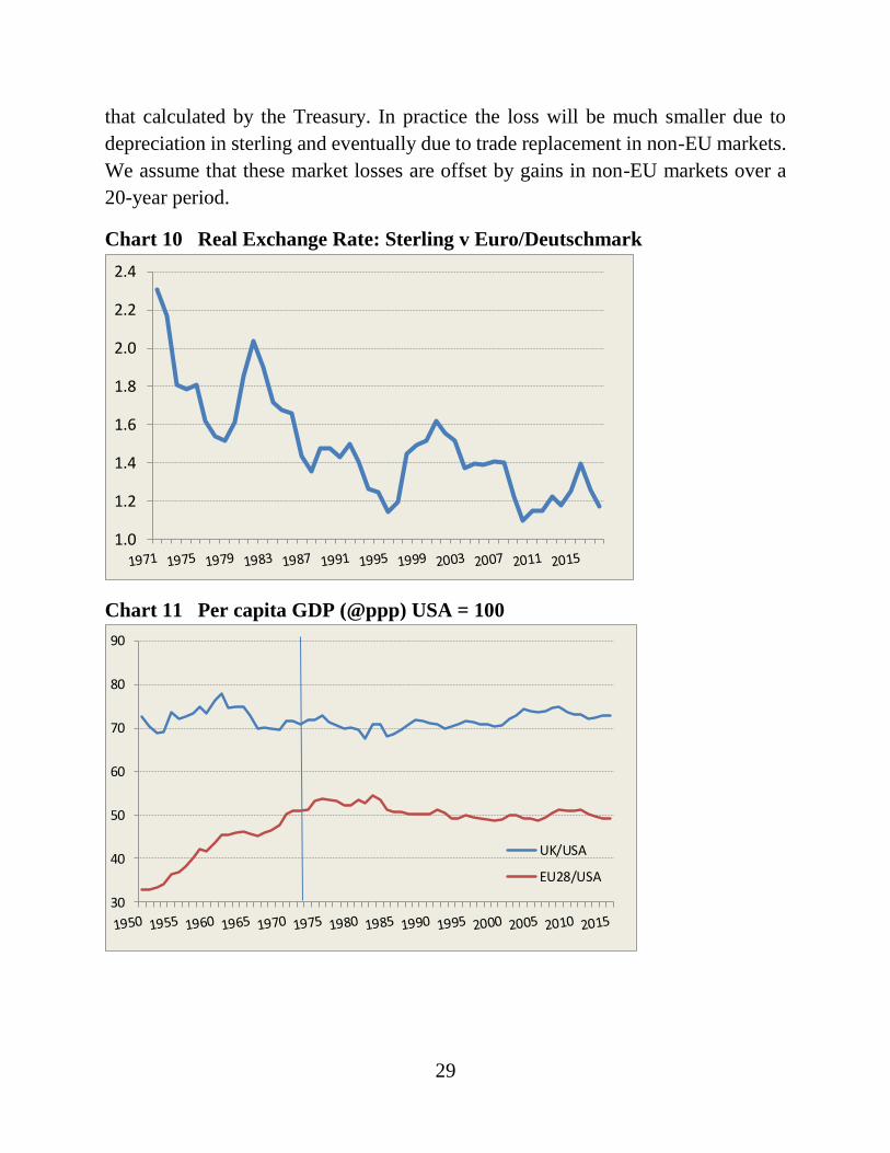
Summary on Trade Assumptions
It seems that much of the large increase in UK trade with the EU has been a
continuation of previous trends and that large increases have also occurred for
exports into the EU from non-member states such as the USA. The share of the EU
as a market for UK exports has been falling fast in the present century and will soon
be below the level of 1973. Another factor is the sterling-euro real exchange rate
which is now about a third lower than was the (Deutschmark) rate in 1973 (Chart
10). With low tariffs and a low exchange rate it seems implausible that Brexit would
result in the large decline in markets calculated by the Treasury.
In the model scenario described below, we will model the Treasury assumption on
trade losses due to Brexit. However, our main Brexit scenario will use a much
smaller reduction in exports. Based on our own gravity model work described in
annex B, we have assumed a potential loss of 20% of EU markets, i.e. under half of
29
that calculated by the Treasury. In practice the loss will be much smaller due to
depreciation in sterling and eventually due to trade replacement in non-EU markets.
We assume that these market losses are offset by gains in non-EU markets over a
20-year period.
Chart 10 Real Exchange Rate: Sterling v Euro/Deutschmark
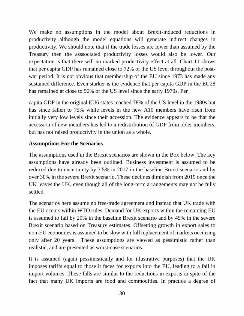
Chart 11 Per capita GDP (@ppp) USA = 100
1.0
1.2
1.4
1.6
1.8
2.0
2.2
2.4
30
40
50
60
70
80
90
UK/USA
EU28/USA
30
We make no assumptions in the model about Brexit-induced reductions in
productivity although the model equations will generate indirect changes in
productivity. We should note that if the trade losses are lower than assumed by the
Treasury then the asssociated productivity losses would also be lower. Our
expectation is that there will no marked productivity effect at all. Chart 11 shows
that per capita GDP has remained close to 72% of the US level throughout the post-
war period. It is not obvious that membership of the EU since 1973 has made any
sustained difference. Even starker is the evidence that per capita GDP in the EU28
has remained at close to 50% of the US level since the early 1970s. Per
capita GDP in the original EU6 states reached 78% of the US level in the 1980s but
has since fallen to 75% while levels in the new A10 members have risen from
initially very low levels since their accession. The evidence appears to be that the
accession of new members has led to a redistribution of GDP from older members,
but has not raised productivity in the union as a whole.
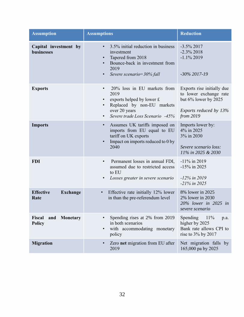
Assumptions For the Scenarios
The assumptions used in the Brexit scenarios are shown in the Box below. The key
assumptions have already been outlined. Business investment is assumed to be
reduced due to uncertainty by 3.5% in 2017 in the baseline Brexit scenario and by
over 30% in the severe Brexit scenario. These declines diminish from 2019 once the
UK leaves the UK, even though all of the long-term arrangements may not be fully
settled.
The scenarios here assume no free-trade agreement and instead that UK trade with
the EU occurs within WTO rules. Demand for UK exports within the remaining EU
is assumed to fall by 20% in the baseline Brexit scenario and by 45% in the severe
Brexit scenario based on Treasury estimates. Offsetting growth in export sales to
non-EU economies is assumed to be slow with full replacement of markets occurring
only after 20 years. These assumptions are viewed as pessimistic rather than
realistic, and are presented as worst-case scenarios.
It is assumed (again pessimistically and for illustrative purposes) that the UK
imposes tariffs equal to those it faces for exports into the EU, leading to a fall in
import volumes. These falls are similar to the reductions in exports in spite of the
fact that many UK imports are food and commodities. In practice a degree of
31
diversion of imports may occur. For instance new world wines displace French,
Italian, Spanish and other EU wines.
We have assumed substantial losses in net FDI flows into the UK. These are flows
of physical investment with direct effects on employment, rather than the financial
flows in the Treasury analysis. The numbers are essentially arbitrary but are based
on the belief that a significant proprtion of FDI enters the UK as a base for accessing
an EU-wide market, and will be less attracted to a UK location once the UK leaves
the EU.
The sterling effective exchange rate has been adjusted so that the average value in
2017 is 12% below the pre-referendum level. No further adjustment is made and the
exchange rate after 2017 is determined by the exchange rate equation in the model.
32
Assumption Assumptions Reduction
Capital investment by
businesses
• 3.5% initial reduction in business
investment
• Tapered from 2018
• Bounce-back in investment from
2019
• Severe scenario=30% fall
-3.5% 2017
-2.3% 2018
-1.1% 2019
-30% 2017-19
Exports • 20% loss in EU markets from
2019
• exports helped by lower £
• Replaced by non-EU markets
over 20 years
• Severe trade Loss Scenario -45%
Exports rise initially due
to lower exchange rate
but 6% lower by 2025
Exports reduced by 13%
from 2019
Imports • Assumes UK tariffs imposed on
imports from EU equal to EU
tariff on UK exports
• Impact on imports reduced to 0 by
2040
Imports lower by:
4% in 2025
3% in 2030
Severe scenario loss:
11% in 2025 & 2030
FDI
• Permanent losses in annual FDI,
assumed due to restricted access
to EU
• Losses greater in severe scenario
-11% in 2019
-15% in 2025
-12% in 2019
-21% in 2025
Effective Exchange
Rate
• Effective rate initially 12% lower
in than the pre-referendum level
8% lower in 2025
2% lower in 2030
20% lower in 2025 in
severe scenario
Fiscal and Monetary
Policy
• Spending rises at 2% from 2019
in both scenarios
• with accommodating monetary
policy
Spending 11% p.a.
higher by 2025
Bank rate allows CPI to
rise to 3% by 2017
Migration • Zero net migration from EU after
2019
Net migration falls by
165,000 pa by 2025
33
Fiscal policy for 2017-18 is taken directly from government plans announced in the
2017 Budget. In these plans spending rises faster than in pre-referendum plans by
close to 1% per annum. We increase this extra spending by closer to 2% in 2019-20,
and continue faster growth by 1% from 2021. Government current and capital
spending on goods and services is consequently 11% higher by 2025 than in the pre-
referendum forecast. Monetary policy is accommodating of higher inflation and the
bank rate is assumed to be kept 1.75 percentage point lower in 2017 than in the pre-
referendum forecast with the gap eliminated by 2020.
Finally, controls on migration from the EU are assumed to be imposed in mid-2019,
leading to net migration falling to around 165,000 from 2020.
Scenario Results
As outlined above we generate two scenarios. Our baseline Brexit scenario uses the
main assumptions in the Box above. The other more severe ‘HMT Brexit’ scenario
uses the Treasury’s calculated impact on trade and short-term uncertainty impacts
which are much higher than those in the baseline Brexit scenario. These assumptions
were entered into the CBR UKMOD model with no further adjustments. The
following sections calculate an estimated impact of Brexit as the difference between
the Brexit scenarios and our pre-referendum forecasts run in June 2016 and with
none of the adjustments listed in the Box. We emphasise again that we regard these
scenarios as pessimistic but illustrative of what could happen. In practice, we expect
a free-trade agreement to emerge between the UK and EU. Since this a continuation
of the status quo it should be easier to negotiate than a completely new FTA such as
the Canada-EU agreement. Political differences may however mean that this takes a
long time to emerge, although it seems likely that transitional arrangements based
on free-trade will be put in place.
34
Real GDP
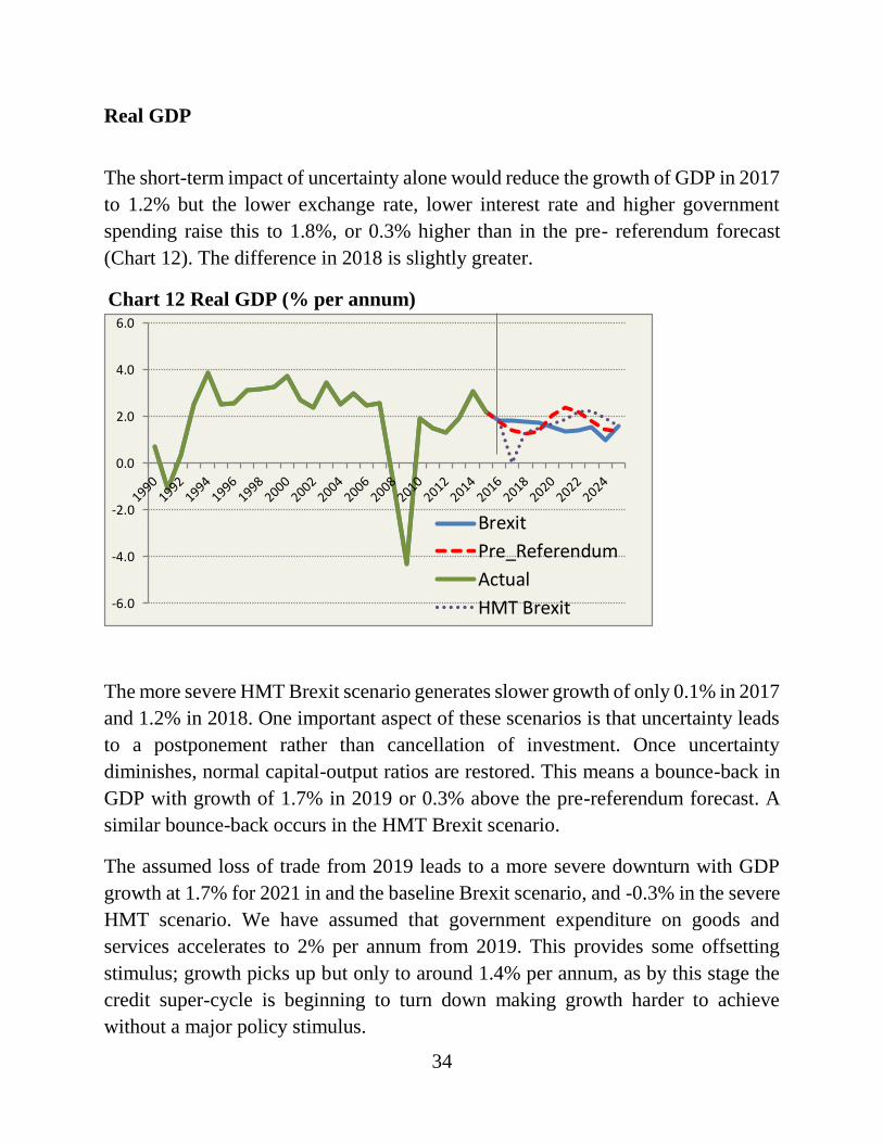
The short-term impact of uncertainty alone would reduce the growth of GDP in 2017
to 1.2% but the lower exchange rate, lower interest rate and higher government
spending raise this to 1.8%, or 0.3% higher than in the pre- referendum forecast
(Chart 12). The difference in 2018 is slightly greater.
Chart 12 Real GDP (% per annum)
-6.0
-4.0
-2.0
0.0
2.0
4.0
6.0
Brexit
Pre_Referendum
Actual
HMT Brexit
The more severe HMT Brexit scenario generates slower growth of only 0.1% in 2017
and 1.2% in 2018. One important aspect of these scenarios is that uncertainty leads
to a postponement rather than cancellation of investment. Once uncertainty
diminishes, normal capital-output ratios are restored. This means a bounce-back in
GDP with growth of 1.7% in 2019 or 0.3% above the pre-referendum forecast. A
similar bounce-back occurs in the HMT Brexit scenario.
The assumed loss of trade from 2019 leads to a more severe downturn with GDP
growth at 1.7% for 2021 in and the baseline Brexit scenario, and -0.3% in the severe
HMT scenario. We have assumed that government expenditure on goods and
services accelerates to 2% per annum from 2019. This provides some offsetting
stimulus; growth picks up but only to around 1.4% per annum, as by this stage the
credit super-cycle is beginning to turn down making growth harder to achieve
without a major policy stimulus.
35
The overall impact in the baseline Brexit scenario is that GDP is a little higher up to
2020 as the lower exchange and interest rates offset the negative impact of
uncertainty. After 2020 the loss of trade results in GDP falling below the pre-
referendum trend, ending up in 2025 some 1.5% below the pre-referendum forecast.
Part of this reduction in GDP comes from lower migration. As a result, there is less
of a fall in per capita GDP which ends up in 2025 at much the same as in the pre-
referendum forecast. The HMT Brexit scenario has a greater loss, at 6% of GDP in
2025. This is close to the Treasury’s 7% for 2030. Once again, the fall in per capita
GDP by 2025 is less in this scenario at 4%. Unlike the NiGEM model our CBR
model predicts a negative impact of migration on productivity measured as per capita
GDP. This is to be expected when the majority of recent immigrants from the EU
come to work initially in minimum wage jobs.
Beyond 2025, the model predicts a pick-up in GDP and per capita GDP as trade
begins to slowly recover. By 2030 both GDP and per capita GDP are above the pre-
referendum forecast. Again, a lower exchange rate and faster growth in government
spending play a role in this recovery. This recovery is broadly sustainable in that the
current account on the balance of payments is more favourable by 2030 than in the
pre-referendum forecast. The government deficit remains low at close to 2% of GDP.
Government debt is substantially higher than in the pre-referendum forecast but does
from 88% in 2017 to 77% in 2030.
Consumer Price Inflation
The one indisputable result of the Brexit Referendum has been a large fall in sterling
relative to most other currencies, although in our view this brings forward a
depreciation that would eventually have occurred albeit more slowly. The long-term
result of this depreciation is expected to be a welcome reduction in the large balance
of payments deficit to a manageable level. The more immediate impact is to increase
the price of imported goods and services leading to a general rise in consumer price
inflation.
36
Chart 13 UK Consumer Price Inflation (% per annum)
0
1
2
3
4
5
6
7
8Brexit
Pre-Referendum
Actual
HMT Brexit
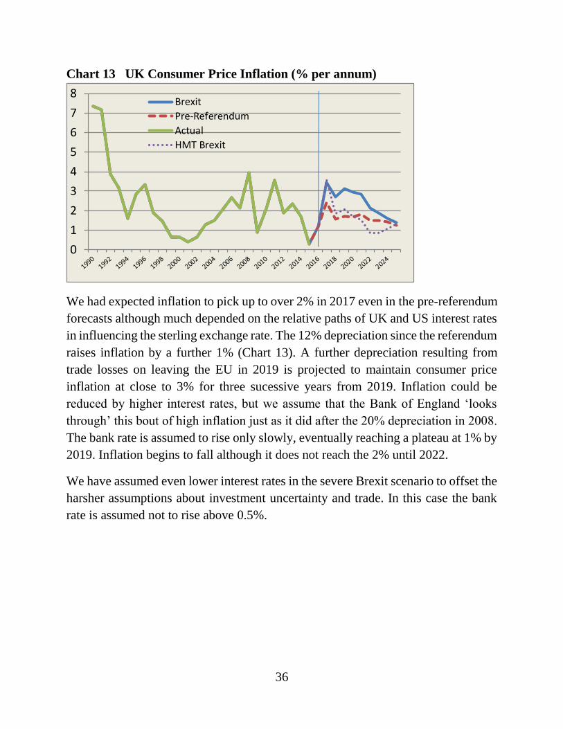
We had expected inflation to pick up to over 2% in 2017 even in the pre-referendum
forecasts although much depended on the relative paths of UK and US interest rates
in influencing the sterling exchange rate. The 12% depreciation since the referendum
raises inflation by a further 1% (Chart 13). A further depreciation resulting from
trade losses on leaving the EU in 2019 is projected to maintain consumer price
inflation at close to 3% for three sucessive years from 2019. Inflation could be
reduced by higher interest rates, but we assume that the Bank of England ‘looks
through’ this bout of high inflation just as it did after the 20% depreciation in 2008.
The bank rate is assumed to rise only slowly, eventually reaching a plateau at 1% by
2019. Inflation begins to fall although it does not reach the 2% until 2022.
We have assumed even lower interest rates in the severe Brexit scenario to offset the
harsher assumptions about investment uncertainty and trade. In this case the bank
rate is assumed not to rise above 0.5%.
37
Real wages
High inflation resulting the sterling depreciation can undermine the real value of
wages, leading in turn to lower consumption and hence lower GDP. Much depends
on whether wages rise in response to higher inflation. Average earnings have risen
by less than 2% per annum in most years since the economic crisis of 2008 and there
is a widespread view among economists that there is a relatively stable 2% per
annum wage norm among employers. Average weekly wages did break this ceiling
in 2013 and 2015 but not by much.
Our equations for earnings suggest that earnings will rise by more than 2% as
employment rates reach a peak in 2017 and especially as migration reduces from
2019. The UK labour market has become very dependent on foreign-born labour
with the increase in foreign-born workers being equivalent to over 80% of additional
employment since 2004. Immigration restrictions will provide the biggest shock to
wage bargaining for over a decade. Even so, we expect real wages to decline gently
until 2020. Nominal wages will fail to keep pace with rising consumer prices but
only by a little. Real wages in 2025 are expected to be only 3% above the level in
2007 shortly after the accession of the EU10 member states to the EU. It is only later
that we expect lower migration to be associated with steady rises in real wages.
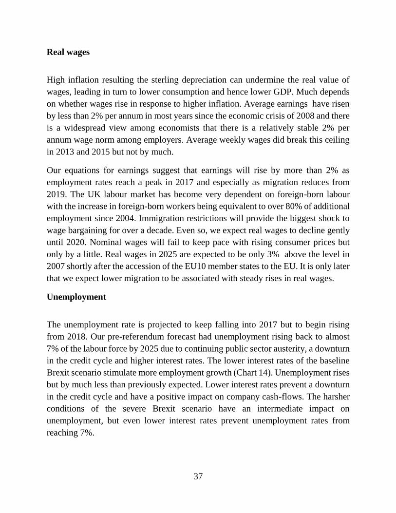
Unemployment
The unemployment rate is projected to keep falling into 2017 but to begin rising
from 2018. Our pre-referendum forecast had unemployment rising back to almost
7% of the labour force by 2025 due to continuing public sector austerity, a downturn
in the credit cycle and higher interest rates. The lower interest rates of the baseline
Brexit scenario stimulate more employment growth (Chart 14). Unemployment rises
but by much less than previously expected. Lower interest rates prevent a downturn
in the credit cycle and have a positive impact on company cash-flows. The harsher
conditions of the severe Brexit scenario have an intermediate impact on
unemployment, but even lower interest rates prevent unemployment rates from
reaching 7%.
38
Chart 14 Unemployment rate (% of labour Force)
3
4
5
6
7
8
9
10
11
Brexit
Pre-Referendum
ACTUAL
HMT Brexit
Public Sector Finances
Public expenditure on goods and services rises 1-2% per annum faster than in our
pre-referendum forecast. With GDP growth generally slower, public sector revenues
are initially lower but improve into the next decade as economic growth picks up
and with savings on contributions to the EU. The values we use for public spending
assume that the EU savings are spent on other things and these are built into the
spending assumptions above. The same spending assumptions are used in both
Brexit scenarios, but tax revenues are lower in the severe scenario due to lower
growth in GDP.
39
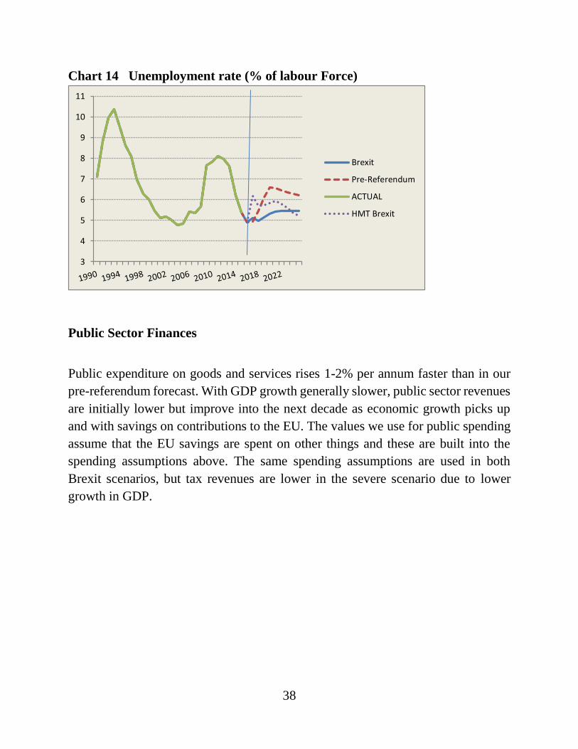
Chart 15 Government Fiscal Deficit (% of GDP)
-2.0
0.0
2.0
4.0
6.0
8.0
10.0
12.0
Actual
Brexit
Pre_referendum
HMT Brexit
In our pre-referendum forecast we had not expected the government’s fiscal defict
to hit the Chancellor’s target of budget balance by 2019-20, but instead to flatline at
around 2.5% of GDP for a few years before continuing a downward trajectory (Chart
15). The Brexit scenarios, not surprisingly, have initially higher deficits. The deficit
in the baseline Brexit scenario remains below 3% of GDP which is low enough keep
aggregate debt on a downward path from 2017 helped by higher price inflation
(Chart 16). Even in the severe scenario the deficit does not rise above 4%, allowing
the debt ratio to fall below its 2016 level by 2025.
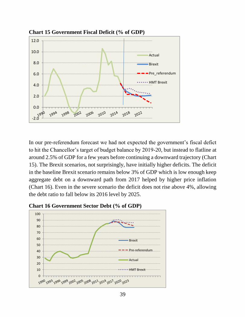
Chart 16 Government Sector Debt (% of GDP)
0
10
20
30
40
50
60
70
80
90
100
Brexit
Pre-referendum
Actual
HMT Brexit
40
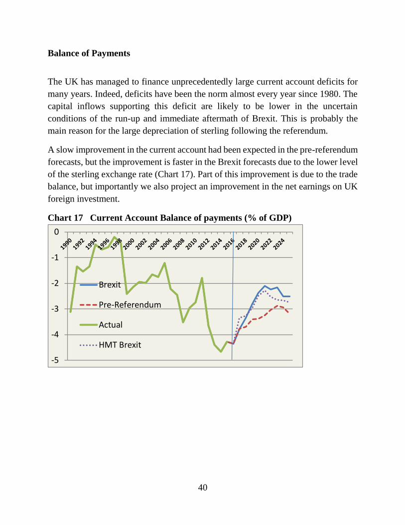
Balance of Payments
The UK has managed to finance unprecedentedly large current account deficits for
many years. Indeed, deficits have been the norm almost every year since 1980. The
capital inflows supporting this deficit are likely to be lower in the uncertain
conditions of the run-up and immediate aftermath of Brexit. This is probably the
main reason for the large depreciation of sterling following the referendum.
A slow improvement in the current account had been expected in the pre-referendum
forecasts, but the improvement is faster in the Brexit forecasts due to the lower level
of the sterling exchange rate (Chart 17). Part of this improvement is due to the trade
balance, but importantly we also project an improvement in the net earnings on UK
foreign investment.
Chart 17 Current Account Balance of payments (% of GDP)
-5
-4
-3
-2
-1
0
Brexit
Pre-Referendum
Actual
HMT Brexit
41
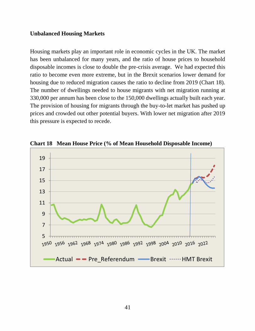
Unbalanced Housing Markets
Housing markets play an important role in economic cycles in the UK. The market
has been unbalanced for many years, and the ratio of house prices to household
disposable incomes is close to double the pre-crisis average. We had expected this
ratio to become even more extreme, but in the Brexit scenarios lower demand for
housing due to reduced migration causes the ratio to decline from 2019 (Chart 18).
The number of dwellings needed to house migrants with net migration running at
330,000 per annum has been close to the 150,000 dwellings actually built each year.
The provision of housing for migrants through the buy-to-let market has pushed up
prices and crowded out other potential buyers. With lower net migration after 2019
this pressure is expected to recede.
Chart 18 Mean House Price (% of Mean Household Disposable Income)
5
7
9
11
13
15
17
19
Actual Pre_Referendum Brexit HMT Brexit
42
Conclusions
A model based largely on equations reflecting past relationships between macro-
economic variables has little to go on in attempting to project a long-term future
outside the EU. Nor is there much on which to base a judgement about how much of
investment and consumption might be delayed or cancelled due to inevitable
uncertainty about the future. Our two scenarios about possible futures leading up to
and following Brexit are based on a series of assumptions not only about what form
trade arrangements might take, but importantly, what impact these changes will have
on the wider economy. We do not feel that it is possible to rely strongly on the
gravity model approach in estimating the impact of EU membership on trade. The
method can generate different results in different formulations and the Treasury’s
use of this approach is inappropriate. The Treasury relies on average impacts across
all EU members and on equations estimated across over a hundred countries most of
them involved in little trade with the UK. The impact on UK exports to the EU is
much smaller. Our attempt to replicate the Treasury analysis with a gravity model
using data with a Poisson estimator to deal with the higher variability among small
countries demonstrates that the UK’s dependence on the EU is much weaker than
the average. The Treasury failed to recognise this and its conclusion must be
regarded as flawed.
We enter this lower trade estimate into our macro-economic model as a baseline
Brexit scenario. Our other scenario examines the impact of the Treasury’s
assumptions even though we feel that these have little basis in reality. The baseline
Brexit scenario builds in things we already know including the depreciation of
sterling and the government’s expenditure plans for the next two years. In this
baseline scenario the loss of GDP peaks at less than 2% in the next decade, after
leaving the EU, before beginning to recover. Postponed investment, loss of EU trade
and lower migration all play a role, but an accommodating monetary policy and a
depreciated currency help to manage the shock, as they should. In per capita terms,
there is never any loss of more than 1%, and in the longer term a substantial gain as
lower cumulative migration exerts an influence. Even under these somewhat
pessimistic assumptions about (temporary) uncertainty and trade losses, the path of
GDP is projected to be only a little lower than it might have been in the absence of
a Leave vote. Inflation is higher but unemployment lower as migration is restrained.

43
The economic outlook is grey rather than black, but this would, in our view, have
been the case with or without Brexit. The deeper reality is the continuation of slow
growth in output and productivity that have marked the UK and other western
economies since the banking crisis. Slow growth of bank credit in a context of
already high debt levels, and exacerbated by public sector austerity prevent
aggregate demand growing at much more than a snail’s pace.
44
Notes
1 H. M. Government (2016) H. M. Treasury Analysis: the Long-term Economic
Impact of EU Membership and the Alternatives, April 2016. Cmnd. 9250. H. M.
Government (2016) H. M. Treasury Analysis: The Immediate Economic Impact of
Leaving the EU. May 2017 Cmnd. 9292
2 H.M.Treasury May 2016 page 8.
3 Office For Budget Responsibility. Economic and Fiscal Outlook. March 2017.
4 HM Treasury (April 2016) op cit.
5 In their milder scenarios the Treasury assume that only half of the gains to trade
from EU membership are reversed since non-tariff barriers in the form of regulatory
differences will initially be limited. In the Treasury’s severe scenario it is assumed
that gains are fully reversed.
6 There is something odd about a gravity model applied to trade in that the amount
of trade between two countries is not constrained by the size of the smaller economy.
Hence the size of the term ln(Yi*Yj) can be the same for trade between say
Luxemburg and the USA as between two medium sized countries even though in the
former case the size of the Luxemburg economy imposes an upper limit on the level
of trade.
7 We have used data from FDI Intelligence, an FT subsidiary, on employment in
FDI projects to estimate the money value of physical projects. The Treasury does
undertake some sensitivity analysis but in our view this will not solve the problem.
8 Glick R and Rose A K (September 2015) Currency Unions and Trade. A Post-
EMU Mea Culpa. NBER Working Paper 21535. In a revised version of this paper
published in March 2016 Glick and Rose repeat the point that different econometric
methodologies deliver different results. In particular, different samples of countries
deliver widely variant results. However, in this paper they adopt a preferred form of
equation which generates a positive impact for membership of the EMU. See Rose
and Glick (March 2016) Currency Unions and Trade. A Post-EMU Re-assessment.
Haas School of Business, University of California, Berkeley.
9 Over the last decade the volume of UK exports to the EU has grown by only 4%
due to stagnation in many Eurozone markets, while exports to non-EU markets have
45
grown by 42%. The Treasury forecast of a future loss of 43% of the EU market
equates with a fall in the EU share from the current level (also of 43%), down to
32% by 2030. This level was last seen (for the same 27 countries) in the early 1960s.
If the falling share of EU markets for UK exports experienced over the last decade
were to continue, the EU share would in any case fall to around 30% even if the UK
stayed fully within the UK. Oxford Economics have undertaken a more precise
calculation and estimates a fall to 32% (see Slater A (2016) Will Brexit Speed a
Seismic Shift in UK Trade Patterns? Oxford Economics Research Briefing. Global
7 Sept 2016).
10
https://www.gov.uk/government/uploads/system/uploads/attachment_data/file/220
968/foi_eumembership_trade.pdf
11 This implies that all exports are standard commodities for which there is a world
price at which all exporters can sell their goods.
12 A convenient source for accessing this database is at
www.stats.ukdataservice.ac.uk
13 For the Baltic States, we assume that exports grew at the same rate as in Poland,
and for Croatia and Slovenia at the same rate as the former Yugoslavia.
14 GDP at purchasing power parity in the EU28 countries grew at an annual average
rate of 4.7% in the period 1950-79 but only at 2.4% over the subsequent 1980-1999
period, falling to 1.1% after the Eurozone was established in 1999.
15 Growth in UK exports to Non-EU28 countries was 3.3% per annum prior to 1976
but only 1.5% per annum in the following 13 years. New Zealand was the most
obvious market affected by UK accession to the EU. NZ exports to the UK fell
sharply and UK exports to NZ fell by three-quarters between 1974 and 1984 and
have remained low ever since.
46
16 Source: The Commonweath Association. The World Economics website
(http://www.worldeconomics.com/papers/Commonwealth_Growth_Monitor_0e53
b963-bce5-4ba1-9cab-333cedaab048.paper) shows that since 1971 the Eurozone has
declined from 22% to 12% of world GDP while the Commonwealth has grown from
10% to 16%.
17 In a Keynesian demand-based system a reduction in government spending would
normally result in slower growth in GDP. In the OBR model medium-term GDP is
determined independently of demand and the link between austerity and slower
growth is broken.
18 These are ECM equations estimated as single regressions, rather than as a system.
19 Monetary Economics: an Integrated Approach to Credit, Money, Income,
Production and Wealth WynneGodley and Marc Lavoie, Palgrave MacMillan, 2007
20 See footnote 10
21 A convenient source is available at: www. ukdataservice.ac.uk. Data on GDP and
population by country is available at Conference Board Total Economy Database,
http://www.conference-oard.org/data/economydatabase/
47
Annex A. The CBR Model of the UK Macro-economy
The CBR model has been developed and refined over the last five years. It was
originally developed in response to the failure of academic and commercial
economic forecasters to foresee or understand the economic crisis of 2008-9 or to
recognise the dangers in the preceding accumulation of debt by the household and
financial sectors. The ‘business as usual’ response of much of the forecasting
industry leaves much to be desired and the nature of the main public sector models
in the UK is, in our view, unfit for several aspects of policy analysis.
The OBR model, which took over from the Treasury model in 2010, when the Office
for Budget Responsibility was set up as an independent body to place official
economic forecasting at arm’s length from Government, has particular problems. In
an attempt to make a predominantly demand-side system into a supply-side model,
the OBR model gives precedence to its projections of productive capacity. This
capacity is projected purely by assumption. The key assumption relates to labour
productivity which is exogenous and usually presumed to grow at close to 2% per
annum despite the fact that there has been virtually no increase in UK productivity
since 2007. In the OBR’s world, next year will always be better. The other, less
important assumption is on the growth of labour supply, and the OBR adopts official
ONS projections with their arbitrary assumptions about future migration flows. To
make the demand system consistent with supply the OBR assume that actual output
will move to achieve full-capacity operation within 3 or 4 years. At times like the
present where the economy is already operating at close to full capacity, the forecast
for GDP is almost exactly just the track of productive capacity. In the latest OBR
Economic and Fiscal Outlook, released in March 2017, the forecast for growth in
real GDP is 2.1% per annum from 2019. In such a system there can be no Keynesian
multiplier and as a result OBR forecasts have been consistently over-optimistic
about tax revenues and hence the Government’s ability to achieve fiscal balance17.
The forecasting model of the Bank of England (in line with other Central Banks) is
a new Keynesian general equilibrium system, with rigorous but unrealistic micro-
economic foundations. This has a poor forecasting record leading to unfortunate
embarrassments for the Governor of the Bank of England. These include the debacle
in 2013 when Mark Carney attempted to introduce a ‘forward guidance’ regime to
48
guide financial markets as to the probable future path for interest rates. The Bank’s
unemployment forecasts which underpinned the regime proved hopelessly
pessimistic and the regime had to be quietly side-lined.
A general equilibrium model is also used by the Revenue and Customs (HMRC) side
of the Treasury. Our dealings with HMRC over the transfer of responsibility for
corporation tax to Northern Ireland showed that use of this model defied common
sense to an extant verging on the bizarre. The model predicted that changes in
corporation tax would lead to rapid adjustments in the capital stock of businesses
with no medium or long-term impact on FDI flows. In reality low corporation tax
rates continue to attract investment year after year as the experience of the Republic
of Ireland has demonstrated for more than half a century. The decisions of successive
Chancellors of the Exchequer to reduce UK corporation tax rates from 30% down to
17% since 2007 suggest that the advice of their own modellers has been
comprehensively ignored.
The CBR Macro-Economic Model (UKMOD)
The CBR model is described in CBR Working Paper 472 at
www.cbr.cam.ac.uk/publications/working-papers. In brief the model consists of
series of econometric equations18 and identities describing how important macro-
economic indicators are related to one another in both the long-term and short-term.
All equations consist of statistically significant relationships estimated from UK data
over recent decades. A Keynesian view of the economic world influences the
relationships selected for inclusion in these equations, but ultimately it is the data
that determines what precisely is included in each equation and with what weights.
There is no overt attempt to insert profit-maximising or other optimising behaviour
into the model except in as far as it is implicit in the equations for such things as
company investment or private-sector employment. Nor is the model precise about
the formation of expectations. Since it is assumed that most expectations are based
on the recent history of the economy these become subsumed within econometric
equations.
Importantly, there is no explicit NAIRU (non-accelerating inflation rate of
unemployment). Instead the estimated equations prevent employment rates rising
49
above historic peaks via higher inflation and rising interest rates. We estimate
equations for various key aggregate price terms based on past behaviour. In practice
these show that price inflation reflects changes in wage and import costs. Wage
inflation in return reflects price inflation and the employment rate. Interest rates also
influence inflation with a two year lag (mainly via their influence on the sterling
exchange rate) but there is no strong tendency in the data in recent decades for
inflation to accelerate when unemployment is below some critical rate as assumed
in many forecasting models. Forecasts and simulations generated with UKMOD
indicate that rises in wage inflation associated with low unemployment (or high
employment rates) can be contained with relatively small increases in short-term
interest rates.
The forecasts generated by the model are conditional on a number of exogenous
variables chiefly reflecting government fiscal policy and economic conditions
outside the UK. Key exogenous variables are:
World trade (weighted by UK markets)
Government fiscal policy plans (tax rates and nominal spending plans)
Short-term interest rate (used as a policy variable to target consumer price
inflation)
Interest rates in USA
Global price of oil and other raw materials.
50
The model is based on the post-Keynesian approach of Wynne Godley described in
‘Monetary Economics’ by Godley and Lavoie 19:
• 4 sector approach: households, companies, government and foreign
(importantly Godley-Lavoie also has a separate monetary/banking sector
which is not yet developed in this model)
• Stock-flow consistent with a tendency for ratios of assets to incomes not to
diverge too far from long-term averages
• Consumer spending depends on borrowing as well as income, assets and
liabilities
• Mark-up pricing (i.e. consumer prices rise with wage and other costs of
production)
• Wages determined as attempts to gain a traditional share of value-added but
constrained by changes in the employment rate.
In its present form the model does not have a banking sector, although lending to
households is modelled. Household borrowing is semi-exogenous determined by an
equation reflecting past experience in the demand for housing loans but with a partial
adjustment mechanism to move from the current situation in which bank lending is
constrained by impaired balance sheets back towards a relatively unconstrained
position.
51
Annex B An Alternative Gravity Model
In the academic literature, there has been an explosion of papers in the past decade
on empirical estimates of trade relationships, using the workhorse of the gravity
model. The basic hypothesis is that trade between any country pair is proportional
to the products of the GDPs of the two countries and is inversely related to some
measure of distance between the country pair – hence the analogy with the
Newtonian theory of gravitation. This approach underpinned the Treasury’s
estimates of the impact of Brexit. The method used residuals from a basic gravity
equation to measure the impact of EU membership on trade flows. The gravity model
approach is used by the Treasury to establish a crucial elasticity for the impact of
EU membership on the size of trade between EU member countries in the years when
both country pairs have been members. The other elasticity, for country pairs where
one country is an EU member, but the other is not, is interpreted as indicating
whether there is a trade diversion effect for the country which joins the EU. Given
the Treasury’s methodology of using the size and significance of these two factors
in estimating the overall loss to UK trade for leaving the EU, the econometric
procedure bears a great deal of weight in the Treasury’s overall assessment.
The Treasury equation was not described in detail but appeared to be based on data
from around 114 countries and 65 years, providing about 390,000 observations in
all. A feature of this large country sample used by the Treasury is that the vast
majority of the sample consists of non-OECD countries. Much of the cross-section
variation is likely to reflect the large differences in GDP per capita and trade between
emerging economies and mature industrial economies. This is important since the
measure of the EU impact depends on the underlying gravity equation. An average
relationship between trade, GDP and distance obtained from such a large range of
countries, most of which do little trade with the UK or the EU, may not be the best
basis for estimating the impact of EU membership on trade flows. Glick and Rose
(2016) show that in the context of membership of the European Monetary Union
(EMU) the number of countries included in the sample makes a large difference to
the results obtained from a gravity model20.
To investigate further the properties of the gravity modelling adopted by HM
Treasury, we have used a similarly large dataset but with a Poisson quasi-likelihood
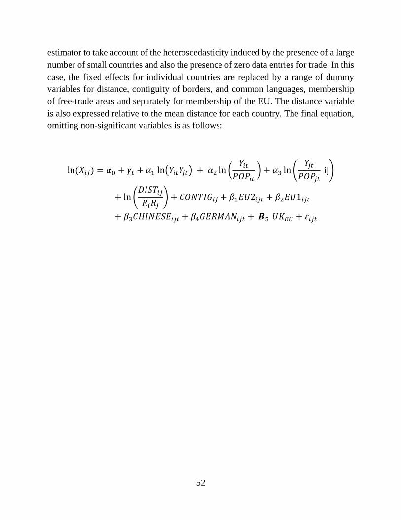
52
estimator to take account of the heteroscedasticity induced by the presence of a large
number of small countries and also the presence of zero data entries for trade. In this
case, the fixed effects for individual countries are replaced by a range of dummy
variables for distance, contiguity of borders, and common languages, membership
of free-trade areas and separately for membership of the EU. The distance variable
is also expressed relative to the mean distance for each country. The final equation,
omitting non-significant variables is as follows:
ln(𝑋𝑖𝑗) = 𝛼0 + 𝛾𝑡 + 𝛼1 ln(𝑌𝑖𝑡𝑌𝑗𝑡) + 𝛼2 ln (𝑌𝑖𝑡
𝑃𝑂𝑃𝑖𝑡 ) + 𝛼3 ln (
𝑌𝑗𝑡
𝑃𝑂𝑃𝑗𝑡 ij)
+ ln (𝐷𝐼𝑆𝑇𝑖𝑗
𝑅𝑖𝑅𝑗) + 𝐶𝑂𝑁𝑇𝐼𝐺𝑖𝑗 + 𝛽1𝐸𝑈2𝑖𝑗𝑡 + 𝛽2𝐸𝑈1𝑖𝑗𝑡
+ 𝛽3𝐶𝐻𝐼𝑁𝐸𝑆𝐸𝑖𝑗𝑡 + 𝛽4𝐺𝐸𝑅𝑀𝐴𝑁𝑖𝑗𝑡 + 𝑩5 𝑈𝐾𝐸𝑈 + 𝜀𝑖𝑗𝑡
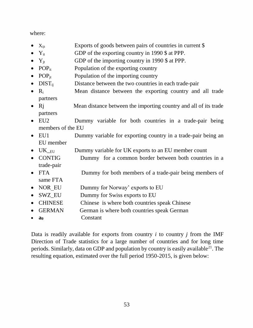
53
where:
Xijt Exports of goods between pairs of countries in current $
Yit GDP of the exporting country in 1990 $ at PPP.
Yjt GDP of the importing country in 1990 $ at PPP.
POPit Population of the exporting country
POPjt Population of the importing country
DISTij Distance between the two countries in each trade-pair
Ri Mean distance between the exporting country and all trade
partners
Rj Mean distance between the importing country and all of its trade
partners
EU2 Dummy variable for both countries in a trade-pair being
members of the EU
EU1 Dummy variable for exporting country in a trade-pair being an
EU member
UK_EU Dummy variable for UK exports to an EU member count
CONTIG Dummy for a common border between both countries in a
trade-pair
FTA Dummy for both members of a trade-pair being members of
same FTA
NOR_EU Dummy for Norway’ exports to EU
SWZ_EU Dummy for Swiss exports to EU
CHINESE Chinese is where both countries speak Chinese
GERMAN German is where both countries speak German
a0 Constant
Data is readily available for exports from country i to country j from the IMF
Direction of Trade statistics for a large number of countries and for long time
periods. Similarly, data on GDP and population by country is easily available21. The
resulting equation, estimated over the full period 1950-2015, is given below:
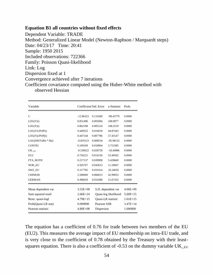
54
Equation B1 all countries without fixed effects
The equation has a coefficient of 0.76 for trade between two members of the EU
(EU2). This measures the average impact of EU membership on intra-EU trade, and
is very close to the coefficient of 0.78 obtained by the Treasury with their least-
squares equation. There is also a coefficient of -0.53 on the dummy variable UK_EU
Dependent Variable: TRADE
Method: Generalized Linear Model (Newton-Raphson / Marquardt steps)
Date: 04/23/17 Time: 20:41
Sample: 1950 2015
Included observations: 722366
Family: Poisson Quasi-likelihood
Link: Log
Dispersion fixed at 1
Convergence achieved after 7 iterations
Coefficient covariance computed using the Huber-White method with
observed Hessian
Variable Coefficient Std. Error z-Statistic Prob.
C -12.96323 0.131690 -98.43779 0.0000
LOG(Yit) 0.851496 0.005066 168.0877 0.0000
LOG(Yjt) 0.862108 0.005124 168.2519 0.0000
LOG(Yit/POPit) 0.449555 0.010018 44.87443 0.0000
LOG(Yjt/POPjt) 0.447144 0.007786 57.43147 0.0000
LOG(DIST/(Rit * Rjt) -0.819123 0.008534 -95.98123 0.0000
CONTIG 0.109109 0.018964 5.753385 0.0000
UK_EU -0.530022 0.028728 -18.44986 0.0000
EU2 0.756215 0.014136 53.49502 0.0000
FTA_BOTH 0.217137 0.039998 5.428669 0.0000
NOR_EU 0.505767 0.043613 11.59667 0.0000
SWZ_EU 0.317785 0.031014 10.24659 0.0000
CHINESE 2.580000 0.060013 42.99053 0.0000
GERMAN 0.496659 0.031686 15.67432 0.0000
Mean dependent var 3.55E+08 S.D. dependent var 4.06E+09
Sum squared resid 2.66E+24 Quasi-log likelihood 5.60E+15
Restr. quasi-logl 4.79E+15 Quasi-LR statistic 1.61E+15
Prob(Quasi-LR stat) 0.000000 Pearson SSR 3.47E+14
Pearson statistic 4.80E+08 Dispersion 1.000000
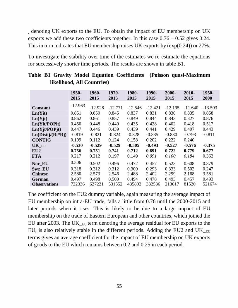
55
, denoting UK exports to the EU. To obtain the impact of EU membership on UK
exports we add these two coefficients together. In this case 0.76 – 0.52 gives 0.24.
This in turn indicates that EU membership raises UK exports by (exp(0.24)) or 27%.
To investigate the stability over time of the estimates we re-estimate the equations
for successively shorter time periods. The results are shown in table B1.
Table B1 Gravity Model Equation Coefficients (Poisson quasi-Maximum
likelihood, All Countries)
1950-
2015
1960-
2015
1970-
2015
1980-
2015
1990-
2015
2000-
2015
2010-
2015
1950-
2000
Constant -12.963 -12.928 -12.771 -12.546 -12.421 -12.195 -11.640 -13.503
Ln(Yit) 0.851 0.850 0.845 0.837 0.831 0.830 0.835 0.858
Ln(Yjt) 0.862 0.861 0.857 0.849 0.844 0.843 0.827 0.876
Ln(Yit/POPit) 0.450 0.448 0.440 0.435 0.428 0.402 0.418 0.517
Ln(Yjt/POPjt) 0.447 0.446 0.439 0.439 0.441 0.429 0.407 0.443
Ln(Distij/(Ri*Rj) -0.819 -0.821 -0.824 -0.828 -0.835 -0.830 -0.793 -0.811
CONTIG 0.109 0.112 0.124 0.158 0.202 0.222 0.240 UK_EU -0.530 -0.529 -0.529 -0.505 -0.493 -0.527 -0.576 -0.375
EU2 0.756 0.751 0.741 0.712 0.691 0.722 0.779 0.677
FTA 0.217 0.212 0.197 0.149 0.091 0.100 0.184 0.362
Nor_EU 0.506 0.502 0.496 0.472 0.457 0.523 0.608 0.379
Swz_EU 0.318 0.312 0.312 0.300 0.293 0.333 0.502 0.247 Chinese 2.580 2.573 2.546 2.488 2.402 2.299 2.168 3.581
German 0.497 0.498 0.500 0.494 0.478 0.493 0.457 0.493
Observations 722336 627221 531552 435802 332536 213617 81520 521674
The coefficient on the EU2 dummy variable, again measuring the average impact of
EU membership on intra-EU trade, falls a little from 0.76 until the 2000-2015 and
later periods when it rises. This is likely to be due to a large impact of EU
membership on the trade of Eastern European and other countries, which joined the
EU after 2003. The UK_EU term denoting the average residual for EU exports to the
EU, is also relatively stable in the different periods. Adding the EU2 and UK_EU
terms gives an average coefficient for the impact of EU membership on UK exports
of goods to the EU which remains between 0.2 and 0.25 in each period.
56
Our conclusion is that the impact of EU membership on UK exports to the EU is
much smaller than the impact reported by the Treasury. The latter was reported as
though it applied to the UK, even though it was estimated as an average across all
EU member states. Our preferred gravity equation is the one reported above with a
Poisson estimator, but the difference in impacts between an EU average and the UK
alone is also observed with the Treasury’s least squares approach. The Treasury
neglected to point out that this was the case, even though they observed this
difference in an earlier (2005) paper.

57


![Macro Economic Theory [Doyle]](https://img.pdfslide.us/doc/110x75/577d20151a28ab4e1e91f26d/macro-economic-theory-doyle.jpg)