Signals and Systems Lab Course - Jacobs University … 3 Signals and Systems Lab, Fall 2013 Outlines ControlFlowFunctions. for, while, if, else, and elseif Example: Oscilloscope Probe

1Introduction Malab

Signals and Systems Lab, Fall 2013

Signals and Systems Lab CourseAdvanced Electrical Engineering Lab Course I (Course Number 300221 )

Mat Lab Introduction

Instructors:

Dr. Dietmar Knipp

Professor or Electrical Engineering

Uwe Pagel

Information: Campusnet

2Introduction Malab


Outlines

What is Matlab?

Matlab Features.

Getting Started with Matlab.

Practical Hints.

From Analog to Digital.

Creating sinusoidal waves using,

1. Matlab commands.

2. Matlab script file.

3. Matlab function file.

3Introduction Malab


Outlines

Control Flow Functions.

for, while, if, else, and elseif

Example: Oscilloscope Probe Frequency Response.

Matlab Toolboxes.

Signal Processing Toolbox.

Complex Functions.

real, imag, complex, conj, abs, and angle

Waveform Generation Functions.

square, sinc, rectpuls, tripuls, and pulstran

4Introduction Malab


What Is MATLAB?

MATLAB is a software package for high performance numerical

computation and visualization.

The name stands for MATrix LABoratory.

The fundamental data-type is the array and the basic building block is the

matrix.

In university environments, it is the standard instructional tool for

introductory and advanced courses in mathematics, engineering, and

science.

In industry, MATLAB is the tool of choice for high-productivity research,

development, and analysis.

5Introduction Malab


Built-in functions User functions

Matlab functions

Matlab programming language

Extra functions

(Tool boxes)

Graphics Computation

C and Fortran

functions

…etc

Matlab's Main Features

External Interface

Matlab functions are optimized for vector operations

6Introduction Malab


Matlab WindowsCommand Window

Figure Window

Edit Window

History Window

7Introduction Malab


Getting help in Matlab

You can launch Matlab help be selecting Help> MATLAB Help. From there

you can easily go to the Matlab function reference and the alphabetical list of

the available functions.

8Introduction Malab


Getting help in Matlab

The easiest and fastest way to get help in Matlab is by using,

The command help and The keyword search lookfor

Type help

Brings out a list of categories in which help is organized.

Type help category

e.g. help elfun gives a list of elementary math functions with the full name of

each function.

Type help function_name

e.g. help sin gives a brief description of the sinusoidal function.

Type Lookfor a descriptive word about the function for which you

need help

e.g. lookfor absolute gives the function abs performing the absolute value.

9Introduction Malab


Creating a directory and saving files

There is a default folder called “work” where Matlab saves the files if no other

location was specified.

If you need to store the files somewhere else,you have to specify the path to

the files or change the working directory of Matlab to the desired directory

using,

The command path The command cd

Type path Shows the Matlab search path

Type cd Shows the current directory

Type addpath C:\mywork Adds the directory mywork to the existing

path

Type rmpath C:\mywork removes the directory mywork from the

current path

Type cd C:\mywork Sets the current directory to C:\mywork

10Introduction Malab


Array,Vector and matrix

What is an array?

What is a vector?

What is a matrix?

All elements can be real or complex numbers using either ‘i’ or ’j’ .

A matrix is written with a square bracket ‘[ ]’ with spaces separating

adjacent columns and semicolons separating adjacent rows.

For examples, consider the following assignments of the variable x.

Real scalar >> x = 5

Complex scalar >> x = 5+10j or x = 5+10i

Row vector >> x = [1 2 3] or [1, 2, 3]

Column vector >> x = [1; 2; 3]

3 x 3 matrix >> x = [1 2 3; 4 5 6; 7 8 9]



Practical Hints

Matlab is case sensitive so "a" and "A" are two different names.

Comment statements are preceded by a “%”.

A semicolon at the end suppresses screen output.

Elements of a matrix or vector can also be accessed.

>>A = [1 2 3; 4 5 6; 7 8 9]

A =

1 2 3

4 5 6

7 8 9

>> x = A(1,3)

x =

3

>> y = A(2,:)

y =

4 5 6

>> z = A(:,3)

z =

3

6

9

>> A= [1 3 6 5 7 8]

A =

1 3 6 5 7 8

>>x=A(2:5)

x =

3 6 5 7

>> A= [1 ;3; 6; 5; 7; 8]A =136578

>>y=A(5:6)y =78



Practical Hints

The command length returns the length of a vector.

>> A= [1 3 6 5 7 8]

A =

1 3 6 5 7 8>> length(A)

ans =

6

You can not add (or subtract) a row vector to a column vector.

Multiplying a vector with a scalar using the arithmetic operator.

What is the difference between arithmetic operator * or / and

the array operator .* or ./ ?

You can multiply (or divide) the elements of two same sized vectors

term by term.

Trigonometric functions as well as elementary math functions operate

on vectors term by term.



Sampling Frequency / Time Vector



What are the different ways of creating vectors?

Using the command t=initial_value:Increment:final_value

t=0:1:10 gives t=[0 1 2 3 4 5 6 7 8 9 10]

Using the built-in function linspace(a,b,n)

t=linspace(0,10,5) gives t=[0 2.5 5 7.5 10]

Using the built-in function logspace(a,b,n)

t=logspace(0,3,4) gives t=[0 10 100 1000]

For vectors of zeros or ones can be created with functions zeros and ones

x=zeros(1,10) creates a 10 element long row vector of 0’s

y=ones(10,1) creates a 10 element long column vector of 1’s



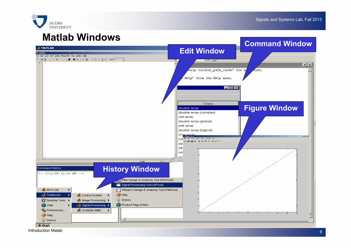
Basic Plotting Commands

MATLAB provides a variety of functions for displaying vector data as line plots

in 2D and 3D, as well as functions for annotating and printing these graphs.

The following table summarizes the functions that produce basic line plots.

These functions differ in the way they scale the plot's axes. Each accepts

input in the form of vectors and automatically scales the axes to

accommodate the data.

Function Description

plot Graph 2-D data with linear scales for both axes

plot3 Graph 3-D data with linear scales for both axes

loglog Graph with logarithmic scales for both axes

semilogx Graph with a logarithmic scale for the x-axis and a

linear scale for the y-axis

semilogy Graph with a logarithmic scale for the y-axis and a

linear scale for the x-axis



Exercise 1: Plot the sinusoidal wave shown below.



File Types

M-filesStandard ASCII text files

.m extension

Two types:

Script files Function files

Mex-filesMatlab-callable Fortran

and C programs

Extension .mex

Mat-filesBinary data files

.mat extension



Scripts Files

Script files are useful when you have to repeat a set of commands

several times.

Script files are sequences of any number of commands, including

commands calling built-in functions or user functions.

Script files can be created using an editor or word processing application,

e.g. notepad (Windows) or the M-file editor (part of the standard Matlab

installation under Windows) and saved as M-files, i.e. using the

extension .m.

To execute a script file,you just have to type the name of the file on the

command line without the extension .m.

Matlab executes the commands one by one as if you have typed all the

commands stored in the file one by one at the command line.

Scripts can operate on existing data in the workspace, i.e. on global

variables, and any variables that they create remain in the workspace.



Script Files

Practical Hints

Never name a script file the same as the name of a variable.

1labcourse.m and labcourse.a1.m are not valid names.

You have to store the script files in the current directory.

If you duplicate script files names, Matlab executes the one that occurs

first in the search path.

Exercise 2:

Create a script file to plot two periods of a sine wave having 4 volts

peak-to-peak amplitude and 800Hz frequency.Save the file under the name

ex2.m and execute it in Matlab.Use the same increment value for creating

the time vector.



Function Files

Function files operate on local variables.

A function file begins with a function definition line,which has a well defined

list of inputs and outputs.The function definition line may look slightly

different depending on whether there is no output, a single output, or

multiple output.

There are two ways a function can be executed

function [y1,y2] = function_name (x1,x2); Function definition line

% add one line describing the function H1 line, Help text

% write online help comments Help text

% your name and date Help text

…………. Function body

[y1,y2] = function_name (x1,x2); With explicit out

function_name (x1,x2); Without any output



Function Files

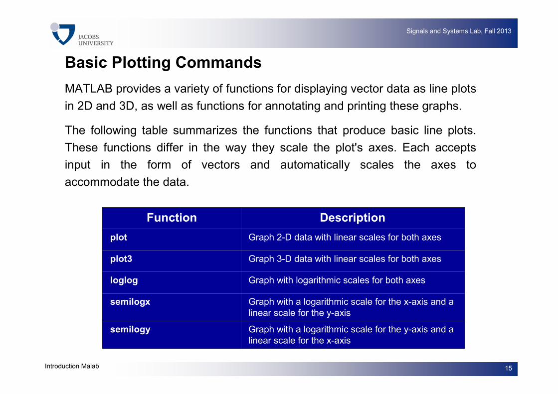
Practical Hints

The first word in the function definition line ‘function' must be typed in lower case.

The function file name and the function name must be the same

You have to store the function files in the current directory.

If you duplicate function names, Matlab executes the one that occurs first

in the search path.

Exercise 3:

Write a function file to plot a sine wave. The peak amplitude, the frequency,

the dc level shift and the number of periods to be plotted are arbitrary.Save the

file under the name ex3.m and execute it to plot 5 periods of a sine wave

having 4 volts peak-to-peak amplitude, 2KHz frequency, and +1.5V dc shift.

Note: For creating the time vector, the increment value should be 0.01T,where

T is the signal period.



Script and function files

Can be easily modifiedCan be easily modified

Have argumentsDo not have arguments

Local variablesGlobal variables

Function filesScript files



Control Flow Functions

for Repeat statements a specific number of times.

while Repeat statements an indefinite number of times

until a condition is no longer satisfied.

for i=1:3

x=i+1

end

x=1;

i=1;

while x < 8

x=2^i

i=i+1

end

x =2

x =3

x =4

x =

2

i =

2

x =

4

i =

3

x =

8

i =

4



Control Flow Functions

if Conditionally execute statements.

else/elseif Conditionally execute statements.

end Terminate for, while, and if statements.

i=5; j=10;

if i>3

k=i

elseif

(i>1)&(j==9)

k=j

else

k=1

end

k =

5



Oscilloscope Probe Frequency Response

Probes are part of your measurement system. Signals travel from the tip

of the probe to the input of the oscilloscope. This signal path makes the

probe an important electrical system component that can affect the

accuracy of the measurement.

Passive probes are specified by bandwidth, attenuation ratio, and

compensation range.




Probes with attenuation X1, X10, or X100, have a tuneable capacitor

that can reduce capacitive effects at the input. The ability to cancel or

minimize effective capacitance improves the probe’s bandwidth.

A simple model describing a passive voltage probe connected to an

oscilloscope consists of a probe capacitance, probe attenuation resistance

together with the oscilloscope input impedance.




Plot output voltage of oszi probe from 10kHz to 1GHz!

C1=10e-12; C2=90e-12; R1=9.0e+6; R2=1.0e+6

RIN=[20 25 30 40 50]; VIN=5;



C1=10e-12;

C2=90e-12;

R1=9.0e+6;

R2=1.0e+6;

RIN=[20 25 30 40 50];

VIN=5;

f=logspace(4,9,100);

for j=1:5

for i=1:100

Z1(i)=1 + j*2*pi*C1*R1*f(i);

Z2(i)=1 + j*2*pi*C2*R2*f(i);

Zin(i)=(R1/Z1(i))+(R2/Z2(i))+(RIN(j));

VOUT(i)=VIN*(R2/Z2(i))/Zin(i);

VOUTABS(i)=abs(VOUT(i));

end


semilogx(f, VOUTABS,'b')

AXIS([10^4 10^9 0.25 0.5])

grid

xlabel('Frequency,Hz');

ylabel('Voltage Amplitude ,V');

title('Frequency Response');

hold on

end



RIN�




Built-in functions User functions

Matlab functions

Matlab programming language

Extra functions

(Tool boxes)

Graphics Computation

C and Fortran

functions

…etc

Matlab's Main Features

External Interface

Matlab functions are optimized for vector operations



Toolboxes

MATLAB features a family of application-specific solutions called toolboxes.

Very important to most users of MATLAB, toolboxes allow you to learn and

apply specialized technology. Toolboxes are comprehensive collections of

MATLAB functions (M-files) that extend the MATLAB environment to solve

particular classes of problems.

Control System Design and Analysis

Control System Toolbox System Identification Toolbox Fuzzy Logic Toolbox

Robust Control Toolbox Model Predictive Control Toolbox

Signal Processing and Communications

Signal Processing Toolbox Communications Toolbox Filter Design Toolbox

Filter Design HDL Coder Wavelet Toolbox Fixed-Point Toolbox RF Toolbox

Link for Code Composer Studio™ Link for ModelSim®

Image Processing

Image Processing Toolbox Image Acquisition Toolbox Mapping Toolbox



Signal Processing Toolbox

The Signal Processing Toolbox contains the following categories of

functions.

Filter Analysis Filter Implementation FIR Digital Filter Design

IIR Digital Filter Design IIR FIlter Order Estimation

Analog Lowpass Filter Prototypes Analog Filter Design

Analog Filter Transformation Filter Discretization

Linear System Transformations Windows Transforms

Cepstral Analysis Statistical Signal Processing and Spectral Analysis

Parametric Modeling Linear Prediction Multirate Signal Processing

Waveform Generation Specialized Operations

Graphical User Interfaces



Complex Functions

In the following we will discuss important functions that belong to elementary

mathematics of complex numbers .

X = real(Z) returns the real part of the complex Z.

Y = imag(Z) returns the imaginary part of the complex Z.

C = complex(a,b) creates a complex output, c, from the two real

inputs.



Complex Functions

ZC = conj(Z) returns the complex conjugate of the complex Z.

x = abs(Z) returns the magnitude of the complex Z,that is

abs(Z) = sqrt(real(Z).^2 + imag(Z).^2)

y = angle(Z) returns the phase angles, in radians, of the complex

Z. The phase angle lies between -π and π.



Waveform Generation Functions

In the following we discuss a list of important functions for waveform generation, which are available as part the signal processing toolbox.

Square Function

x = square (t)

Generates a square wave with period 2π for the elements of time vector t.

x = square (t,duty)

Generates a square wave with specified duty cycle, duty.

Exercise 1: Plot a square wave having 20% duty cycle over the domain -4π ≤ t ≤ 4π.



Exercise 2: Plot a sinc wave for a linearly spaced vector with values ranging from -8 to 8.


Sinc function

y = sinc (x)

computes the mathematical sinc function for an input vector or matrix x.

The sinc function is

The sinc function has a value of 1 where x is zero, and a value of

for all other elements of x.

( ) ( )

≠ππ

==

0x,x

xsin

0x,1

xcsin

( )x

xsin

ππ




Rectangular function

-0.5 0 0.5

1

time

rect (t)

-t0 0

a

T

time

rect (t)

( ) ( )

>

≤==

5.0t,0

5.0t,1trectts

( )

>+

≤+

=

+⋅=

5.0T

tt,0

5.0T

tt,a

T

ttrectats

0

0

0

Normalized continuous time rectangular pulse function

Scaled, and time-shifted continuous time rectangular pulse

function




y = rectpuls (t)

returns a continuous, aperiodic, unity-height rectangular pulse at the sample

times indicated in array t, centered about t = 0 and with a default width of 1.

y = rectpuls (t,w)

generates a rectangle of width w.

rectpuls is typically used in conjunction with the pulse train

generating function pulstran

Exercise 3: Plot a continuous time rectangular pulse having 3V amplitude and pulse width of 5 over the domain -4π ≤ t ≤ 4π.The pulse is time-shifted by 2 in the direction of the positive axis.




Triangular function

( ) ( )

>

≤−=Λ=

1,0

11

t

tttts

1

-1 0 1

time

triangle (t)

Normalized continuous time triangular function

y = tripuls (T)

returns a continuous, aperiodic, symmetric, unity-height triangular pulse at the

times indicated in array T, centered about T=0 and with a default width of 1.

y = tripuls (T,w)

generates a triangular pulse of width w.




Triangular function (Continue)

y = tripuls (T,w,s)

generates a triangular pulse with skew s, where -1 < s < 1. When s is 0, a

symmetric triangular pulse is generated.

tripuls is typically used in conjunction with the pulse train

generating function pulstran

Exercise 4: Plot a continuous time triangular pulse having 2V amplitude and pulse width of 4 over the domain -4π ≤ t ≤ 4π.The pulse is time-shifted by 1 in the direction of the negative axis.




Pulse Train

y = pulstran (t,d,'func')

generates a pulse train based on samples of a continuous function, 'func',

where 'func' is

'rectpuls', for generating a sampled aperiodic rectangle

'tripuls', for generating a sampled aperiodic triangle

pulstran is evaluated length(d) times and returns the sum of the evaluations

y = func(t-d(1)) + func(t-d(2)) + ...

The function is evaluated over the range of argument values specified in

array t, after removing a scalar argument offset taken from the vector d.




An optional gain factor may be applied to each delayed evaluation by specifying

d as a two-column matrix, with the offset defined in column 1 and associated

gain in column 2 of d. Note that a row vector will be interpreted as specifying

delays only.

Pulstran (t,d,'func',p1,p2,...)

allows additional parameters to be passed to 'func' as necessary.

For example:

func(t-d(1),p1,p2,...) + func(t-d(2),p1,p2,...) + ...



Exercise 5:

Generate a symmetric triangular wave with a repetition rate of 4 Hz and pulse

width of 0.1s. The triangular wave has a length of 1s and 1 kHz sampling

frequency. The repetition amplitude should attenuate by 0.5 each time.

Exercise 6:

Using the same Matlab commands used in exercise 5, modify the code to

generate a sawtooth wave instead of a triangular wave



Exercise 7:

Using the ‘pulstran’ function , plot an impulse train signal of length 1s. The

repetition rate of the impulse train signal is 5Hz. The impulse has 50ms impulse

width and 500 Hz sampling frequency. The amplitude of the impulses should be

5V.The impulse train signal is superimposed by random noise (Rand) of 0.5 as

a maximum noise value.



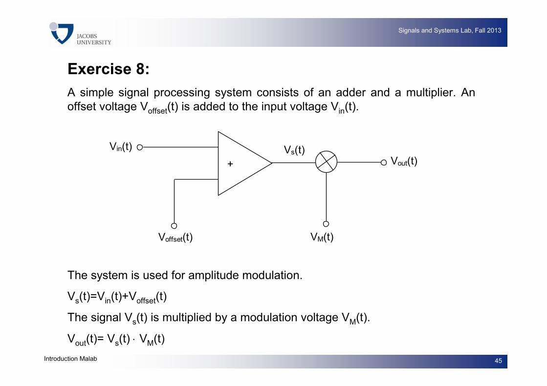
Exercise 8:

A simple signal processing system consists of an adder and a multiplier. An

offset voltage Voffset(t) is added to the input voltage Vin(t).

The system is used for amplitude modulation.

Vs(t)=Vin(t)+Voffset(t)

The signal Vs(t) is multiplied by a modulation voltage VM(t).

Vout(t)= Vs(t) ⋅ VM(t)

Voffset(t)

Vin(t)

+

VM(t)

Vs(t) Vout(t)



The input signal is given by

Vin(t)=V0⋅cos(2πt/Tin), V0=2V, Tin=0.2ms

The modulation voltage is described by

VM(t)=cos(2πt/TM), TM=10µs

The offset voltage Voff(t) is constant over time and described by:

Voffset=2V0=const.

(a) Create the signals Vs(t) and Vout(t).The two signals should be together

on the same plot.

(b) Use subplot to plot the four signals Vin(t), VM(t), Vs(t), and Vout(t).

(c) The offset voltage is reduced to Voffset2(t)=1.5.V0 ,Voffset3(t)=V0 and

Voffset4(t)=0.5.V0 .Use subplot to plot the output signals for the four

cases. Export the plot as JPEG image.



Tasks

Read the safety instructions and sign the safety agreement.

The agreement will be collected next week.

Prepare Experiment 1 , Part A, RLC Transient Response.

Documents

Signals and Systems Lab Course - Jacobs University … 3 Signals and Systems Lab, Fall 2013 Outlines ControlFlowFunctions. for, while, if, else, and elseif Example: Oscilloscope Probe