Embed Size (px)
Citation preview

LECTURE NOTES IN LOGIC
YIANNIS N. MOSCHOVAKIS
March 29, 2014


CONTENTS
Chapter 1. First order logic . . . . . . . . . . . . . . . . . . . . . . . . . . . . . . . . . . 11A. Examples of structures. . . . . . . . . . . . . . . . . . . . . . . . . . . . . . . . . . . . . . 11B. The syntax of First Order Logic (FOL) . . . . . . . . . . . . . . . . . . . . . 41C. Semantics of FOL . . . . . . . . . . . . . . . . . . . . . . . . . . . . . . . . . . . . . . . . . . 91D. First order definability . . . . . . . . . . . . . . . . . . . . . . . . . . . . . . . . . . . . . . 151E. Arithmetical functions and relations . . . . . . . . . . . . . . . . . . . . . . . . 171F. Quantifier elimination . . . . . . . . . . . . . . . . . . . . . . . . . . . . . . . . . . . . . . 221G. Theories and elementary classes . . . . . . . . . . . . . . . . . . . . . . . . . . . . . 291H. The Hilbert proof system for FOL . . . . . . . . . . . . . . . . . . . . . . . . . . 341I. The Completeness Theorem. . . . . . . . . . . . . . . . . . . . . . . . . . . . . . . . . 381J. The Compactness and Skolem-Lowenheim Theorems . . . . . . . . 441K. Some other languages . . . . . . . . . . . . . . . . . . . . . . . . . . . . . . . . . . . . . . . 461L. Problems for Chapter 1 . . . . . . . . . . . . . . . . . . . . . . . . . . . . . . . . . . . . . 48
Chapter 2. Some results from model theory . . . . . . . . . . . . . . . . 572A. Elementary embeddings and substructures . . . . . . . . . . . . . . . . . . 572B. The downward Skolem-Lowenheim Theorem . . . . . . . . . . . . . . . . 632C. Types . . . . . . . . . . . . . . . . . . . . . . . . . . . . . . . . . . . . . . . . . . . . . . . . . . . . . . 662D. Back-and-forth games. . . . . . . . . . . . . . . . . . . . . . . . . . . . . . . . . . . . . . . 802E. ∃1
1 on countable structures . . . . . . . . . . . . . . . . . . . . . . . . . . . . . . . . . . 912F. Craig interpolation and Beth definability (via games) . . . . . . . 100
Chapter 3. Introduction to the theory of proofs . . . . . . . . . . 1053A. The Gentzen Systems . . . . . . . . . . . . . . . . . . . . . . . . . . . . . . . . . . . . . . . 1053B. Cut-free proofs . . . . . . . . . . . . . . . . . . . . . . . . . . . . . . . . . . . . . . . . . . . . . 1113C. Cut Elimination . . . . . . . . . . . . . . . . . . . . . . . . . . . . . . . . . . . . . . . . . . . . 1123D. The Extended Hauptsatz . . . . . . . . . . . . . . . . . . . . . . . . . . . . . . . . . . . 1163E. The propositional Gentzen systems . . . . . . . . . . . . . . . . . . . . . . . . . 1183F. Craig Interpolation and Beth definability (via proofs) . . . . . . . 1203G. The Hilbert program. . . . . . . . . . . . . . . . . . . . . . . . . . . . . . . . . . . . . . . . 1253H. The finitistic consistency of Robinson’s Q . . . . . . . . . . . . . . . . . . . 1263I. Primitive recursive functions . . . . . . . . . . . . . . . . . . . . . . . . . . . . . . . . 128
i

ii CONTENTS
3J. Further consistency proofs . . . . . . . . . . . . . . . . . . . . . . . . . . . . . . . . . . 1333K. Problems for Chapter 3 . . . . . . . . . . . . . . . . . . . . . . . . . . . . . . . . . . . . . 136
Chapter 4. Incompleteness and undecidability . . . . . . . . . . . . . . 1394A. Tarski and Godel (First Incompleteness Theorem). . . . . . . . . . . 1394B. Numeralwise representability in Q . . . . . . . . . . . . . . . . . . . . . . . . . . 1454C. Rosser, more Godel and Lob . . . . . . . . . . . . . . . . . . . . . . . . . . . . . . . . 1504D. Computability and undecidability . . . . . . . . . . . . . . . . . . . . . . . . . . . 1574E. Computable partial functions . . . . . . . . . . . . . . . . . . . . . . . . . . . . . . . 1644F. The basic undecidability results . . . . . . . . . . . . . . . . . . . . . . . . . . . . . 1714G. Problems for Chapter 4 . . . . . . . . . . . . . . . . . . . . . . . . . . . . . . . . . . . . . 175
Chapter 5. Introduction to computability theory . . . . . . . . . 1815A. Semirecursive relations. . . . . . . . . . . . . . . . . . . . . . . . . . . . . . . . . . . . . . 1815B. Recursively enumerable sets. . . . . . . . . . . . . . . . . . . . . . . . . . . . . . . . . 1865C. Productive, creative and simple sets. . . . . . . . . . . . . . . . . . . . . . . . . 1925D. The Second Recursion Theorem. . . . . . . . . . . . . . . . . . . . . . . . . . . . . 1955E. The arithmetical hierarchy . . . . . . . . . . . . . . . . . . . . . . . . . . . . . . . . . . 1985F. Relativization. . . . . . . . . . . . . . . . . . . . . . . . . . . . . . . . . . . . . . . . . . . . . . . 2035G. Effective operations . . . . . . . . . . . . . . . . . . . . . . . . . . . . . . . . . . . . . . . . . 2095H. Problems for Chapter 5 . . . . . . . . . . . . . . . . . . . . . . . . . . . . . . . . . . . . . 214
Chapter 6. Introduction to formal set theory . . . . . . . . . . . . . 2216A. The intended universe of sets . . . . . . . . . . . . . . . . . . . . . . . . . . . . . . . 2216B. ZFC and its subsystems . . . . . . . . . . . . . . . . . . . . . . . . . . . . . . . . . . . . . 2246C. Set theory without powersets, AC or foundation, ZF− . . . . . . 2296D. Set theory without AC or foundation, ZF . . . . . . . . . . . . . . . . . . . 2456E. Cardinal arithmetic and ultraproducts, ZFC . . . . . . . . . . . . . . . . . 2506F. Problems for Chapter 6 . . . . . . . . . . . . . . . . . . . . . . . . . . . . . . . . . . . . . 258
Chapter 7. The constructible universe . . . . . . . . . . . . . . . . . . . . . . 2677A. Preliminaries and the basic definition . . . . . . . . . . . . . . . . . . . . . . . 2677B. Absoluteness. . . . . . . . . . . . . . . . . . . . . . . . . . . . . . . . . . . . . . . . . . . . . . . . 2767C. The basic facts about L . . . . . . . . . . . . . . . . . . . . . . . . . . . . . . . . . . . . . 2857D. ♦ . . . . . . . . . . . . . . . . . . . . . . . . . . . . . . . . . . . . . . . . . . . . . . . . . . . . . . . . . . . 2917E. L and Σ1
2 . . . . . . . . . . . . . . . . . . . . . . . . . . . . . . . . . . . . . . . . . . . . . . . . . . . 2967F. Problems for Chapter 7 . . . . . . . . . . . . . . . . . . . . . . . . . . . . . . . . . . . . . 303
Appendix to Chapters 1 – 5 . . . . . . . . . . . . . . . . . . . . . . . . . . . . . . . . . . . . . 1
Additional problems for 220B . . . . . . . . . . . . . . . . . . . . . . . . . . . . . . . . . . 1
Informal notes, full of errors, March 29, 2014, 15:45 ii
CHAPTER 1
FIRST ORDER LOGIC
Our main aim in this fist chapter is to introduce the basic notions of logicand to prove Godel’s Completeness Theorem 1I.1, which is the first, fun-damental result of the subject. Along the way to motivating, formulatingprecisely and proving this theorem, we will also establish some of the basicfacts of Model Theory, Proof Theory and Recursion Theory, three of themain parts of logic. (The fourth is Set Theory.)
1A. Examples of structures
The language of First Order Logic is interpreted in mathematical struc-tures, like the following.
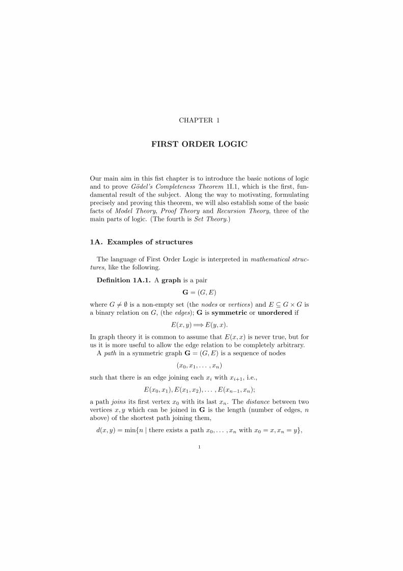
Definition 1A.1. A graph is a pair
G = (G, E)
where G 6= ∅ is a non-empty set (the nodes or vertices) and E ⊆ G×G isa binary relation on G, (the edges); G is symmetric or unordered if
E(x, y) =⇒E(y, x).
In graph theory it is common to assume that E(x, x) is never true, but forus it is more useful to allow the edge relation to be completely arbitrary.
A path in a symmetric graph G = (G,E) is a sequence of nodes
(x0, x1, . . . , xn)
such that there is an edge joining each xi with xi+1, i.e.,
E(x0, x1), E(x1, x2), . . . , E(xn−1, xn);
a path joins its first vertex x0 with its last xn. The distance between twovertices x, y which can be joined in G is the length (number of edges, nabove) of the shortest path joining them,
d(x, y) = minn | there exists a path x0, . . . , xn with x0 = x, xn = y,
1

2 1. First order logic
and (by convention) it is 0 from a vertex to itself, d(x, x) = 0, and ∞ ifx 6= y and there is no path from x to y. The diameter of a symmetricgraph is the largest distance between two vertices, if there is a maximumdistance, otherwise it is ∞:
diam(G) = supd(x, y) | x, y ∈ G.A symmetric graph is connected if any two distinct points in it are
joined by a path, otherwise it is disconnected.
Definition 1A.2. A partial ordering is a pair
P = (P,≤),
where P is a non-empty set and ≤ is a binary relation on P satisfying thefollowing conditions:
1. For all x ∈ P , x ≤ x (reflexivity).2. For all x, y, z ∈ P , if x ≤ y and y ≤ z, then x ≤ z (transitivity).3. For all x, y ∈ P , if x ≤ y and y ≤ x, then x = y (antisymmetry).A linear ordering is a partial ordering in which every two elements are
comparable, i.e., such that4. for all x, y ∈ P , either x ≤ y or y ≤ x.A wellordering is a linear ordering (U,≤) in which every non-empty
subset has a least element: i.e., for every X ⊆ U , if X 6= ∅, then thereexists some x0 ∈ X such that for all x ∈ X,x0 ≤ x.
Definition 1A.3. The structure of arithmetic or the natural num-bers is the tuple
N = (N, 0, S, +, ·)where N = 0, 1, 2, . . . is the set of (non-negative) integers and S, +, ·are the operations of successor, addition and multiplication on N. Thestructure N has the following characteristic properties:(1) The successor function S is an injection, i.e.,
S(x) = S(y)=⇒x = y,
and 0 is not a successor, i.e., for all x, S(x) 6= 0.(2) For all x, y, x + 0 = x and x + S(y) = S(x + y).(3) For all x, y, x · 0 = 0 and x · S(y) = x · y + x.(4) The Induction Principle: for every set of numbers X ⊆ N, if 0 ∈ X
and for every x, x ∈ X =⇒S(x) ∈ X, then X = N.These properties (or sometimes just (1) and (4)) are called the Peano Ax-ioms for the natural numbers.
Definition 1A.4. A field is a structure of the form
K = (K, 0, 1, +, ·)
Informal notes, full of errors, March 29, 2014, 15:45 2

1A. Examples of structures 3
where 0, 1 ∈ K, + and · are binary operations on K and the following fieldaxioms are true.
(1) (K, 0,+) is a commutative group, i.e., the following hold:1. For all x, x + 0 = x.2. For all x, y, z, x + (y + z) = (x + y) + z.3. For all x, y, x + y = y + x.4. For each x there exists some y such that x + y = 0.(2) 1 6= 0 and for all x, x · 0 = 0, x · 1 = x.(3) The structure (K \0, 1, ·) is a commutative group, and in particular
x, y 6= 0 =⇒x · y 6= 0.
Together with (2), this means that for all x, y in K,
x · y = 0 ⇐⇒ x = 0 or y = 0.
(4) For all x, y, z, x · (y + z) = x · y + x · z (the distributive law).Basic examples of fields are the rational numbers Q, the real numbers R
and the complex numbers C, with universes Q,R,C respectively and theusual operations on these number sets.
Definition 1A.5. The universe of sets is the structure
V = (V,∈)
where V is the collection of all sets and ∈ is the binary relation of member-ship. We list here the most common set of axioms usually assumed aboutsets, not in the simplest way, but directly in terms of the basic membershiprelation, without introducing any auxiliary notions.(1) Extensionality: two sets are equal exactly when they have the same
members, in symbols:
x = y ⇐⇒ (∀u)[u ∈ x ⇐⇒ u ∈ y].
(2) Emptyset and Pairing: there exists a set ∅ with no members, and forany two sets x, y, there is a set z whose members are exactly x and y,i.e., for all u,
u ∈ z ⇐⇒ u = x or u = y.
(3) Union: for each set x there exists a set z whose members are themembers of members of x, i.e., for all u
u ∈ z ⇐⇒ (∃y ∈ x)[u ∈ y].
(4) Power: for each set x there exists a set z whose members are all thesubsets of x, i.e., for all u,
u ∈ z ⇐⇒ (∀v ∈ u)[v ∈ x].
Informal notes, full of errors, March 29, 2014, 15:45 3

4 1. First order logic
(5) Subsets: for each set x and each “definite condition” P (u) on sets,there exists a set z whose members are the members of x which satisfyP (u), i.e., for all u,
u ∈ z ⇐⇒ u ∈ x and P (u).
(6) Infinity: there exists a set z such that ∅ ∈ z and z is closed under the“singleton operation”, i.e., for every x,
x ∈ z =⇒x ∈ z.
(7) Choice: for every set x whose members are all non-empty and pairwisedisjoint, there exists a set z which intersects each member of x inexactly one point, i.e., if y ∈ x, then there exists exactly one u suchthat u ∈ y and also u ∈ z.
(8) Replacement: for every set x and every “definite operation” F whichassigns a set F (v) to every set v, the image F [x] of x by F is a set,i.e., there exists a set z such that for all u,
u ∈ z ⇐⇒ (∃v ∈ x)[u = F (v)].
(9) Foundation: every non-empty set x has a member z from which it isdisjoint, i.e., there is no u ∈ X such that also u ∈ z.
We will not take up seriously the study of set theory until Chapters 6 and7. We need, however, right away, some basic, elementary and mostly well-known facts about sets which are routinely used in all areas of mathematics;some of these are summarized in the Appendix to Chapters 1 – 5.
1B. The syntax of First Order Logic (FOL)
The name FOL abbreviates First Order Logic. It is actually a familyof languages FOL(τ), one for each vocabulary τ , where τ provides namesfor the distinguished elements, relations and functions of the structures wewant to talk about.FOL is also known as Lower Predicate Calculus (with Identity), or Ele-
mentary Logic with Identity or just Elementary Logic.
Definition 1B.1. A vocabulary or signature is a quadruple
τ = (Const, Rel,Funct, arity),
where the sets of constant symbols Const, relation symbols Rel, and functionsymbols Funct have no common members and
arity : Rel ∪ Funct → 1, 2, . . . .A relation or function symbol P is n-ary if arity(P ) = n. We will oftenassume that these sets of names are finite (as they are in the examples
Informal notes, full of errors, March 29, 2014, 15:45 4

1B. The syntax of First Order Logic (FOL) 5
above), but it is convenient and useful to allow them to be arbitrary sets inthe general case; and we should also keep in mind that any one—or all—of these sets may be empty. When they are all finite, we usually exhibitsignatures by enumerating their symbols: for example,
τg = (E) (with E binary)
is a signature for graphs;
τa = (0, S, +, .)
is a signature for arithmetic (with 0 a constant, S a unary function symboland +, · binary function symbols);
τf = (0, 1, +, ·)(with the appropriate arities) is a signature for fields; and
τ∈ = (∈)
(with ∈ binary) is a signature for universe of sets. (We say a rather thanthe signature because the “symbols” R,S, +,∈ etc. are arbitrary.)
Definition 1B.2. The alphabet of the first order language with iden-tity FOL(τ) comprises the symbols in the vocabulary τ and the following,additional symbols which are common to all FOL(τ).
1. The logical symbols ¬ & ∨ → ∀ ∃ =2. The punctuation symbols ( ) ,3. The (individual) variables: v0, v1, v2, . . .
Here ¬ (not), & (and), ∨ (or) and → (implies) are the propositionalsymbols, and ∀ (for all) and ∃ (there exists) are the quantifiers.
Words are finite strings (sequences) of symbols and lh(α) is the lengthof the word α. We use ≡ to denote identity of strings,
α ≡ β ⇐⇒df α and β are the same string.
We also setα v β ⇐⇒df α is an initial segment of β,
so that e.g., ∀v0 v ∀v0R(v0). The concatenation of two strings αβ is thestring produced by putting them together, with α first, so that α v αβ.
Definition 1B.3 (Terms and formulas). Terms are defined by the re-cursion: (a) Each variable is a term. (b) Each constant symbol is a term. (c)If t1, . . . , tn are terms and f is an n-ary function symbol, then f(t1, . . . , tn)is a term. In abbreviated notation:
t :≡ v | c | f(t1, . . . , tn),
where | is read as “or”.
Informal notes, full of errors, March 29, 2014, 15:45 5

6 1. First order logic
Formulas are defined by the recursion: (a) If s, t are terms, then s = tis a formula. (b) If t1, . . . , tn are terms and R is an n-ary relation symbol,then R(t1, . . . , tn) is a formula. (c) If φ, ψ are formulas and v is a variable,then the following are formulas:
¬(φ) (φ) → (ψ) (φ) & (ψ) (φ) ∨ (ψ) ∀vφ ∃vφ
In abbreviated form,
χ :≡ s = t | R(t1, . . . , tn) (the prime formulas)
| ¬(φ) | (φ) → (ψ) | (φ) & (ψ) | (φ) ∨ (ψ) | ∀vφ | ∃vφ
For the rigorous interpretations of these recursive definitions of sets seeProblem app3.
A formula is quantifier free if neither of the quantifier symbols ∃, ∀occurs in it. A formula is in prenex normal form (prenex ) if it lookslike
φ ≡ Q1x1 · · ·Qnxnψ
where each Qi is ∀ or ∃, each xj is a variable and ψ is quantifier free.Terms and formulas are collectively called (well formed) expressions.
Proposition 1B.4 (Parsing for terms). Each term t satisfies exactly oneof the following three conditions.
1. t ≡ v for a uniquely determined variable v.2. t ≡ c for a uniquely determined constant c.3. t ≡ f(t1, . . . , tn) for a uniquely determined function symbol f and
uniquely determined terms t1, . . . , tn.
Proposition 1B.5 (Parsing for formulas). Each formula χ satisfies ex-actly one of the following conditions.
1. χ ≡ s = t for uniquely determined terms s, t.2. χ ≡ R(t1, . . . , tn) for a uniquely determined relation symbol R and
uniquely determined terms t1, . . . , tn.3. χ ≡ ¬(φ) for a uniquely determined formula φ.4. χ ≡ (φ) & (ψ) for uniquely determined formulas φ, ψ.5. χ ≡ (φ) ∨ (ψ) for uniquely determined formulas φ, ψ.6. χ ≡ (φ) → (ψ) for uniquely determined formulas φ, ψ.7. χ ≡ ∃vφ for a uniquely determined variable v and a uniquely deter-
mined formula φ.8. χ ≡ ∀vφ for a uniquely determined variable v and a uniquely deter-
mined formula φ.
These propositions allow us to prove properties of expressions by struc-tural induction, i.e., induction on the length of expressions; and we can
Informal notes, full of errors, March 29, 2014, 15:45 6

1B. The syntax of First Order Logic (FOL) 7
also give definitions by structural recursion, i.e., recursion on the lengthof expressions, cf. Problem app4.
Definition 1B.6 (Free and bound variables). Every occurrence of a vari-able in a term is free. The free occurrences of variables in formulas aredefined by structural recursion as follows.
1. FO(s = t) = FO(s) ∪ FO(t),FO(R(t1, . . . , tn)) = FO(t1) ∪ · · · ∪ FO(tn)
2. FO(¬(φ)) = FO(φ), FO((φ) & (ψ)) = FO(φ) ∪ FO(ψ), and similarlyfor the other connectives.
3. FO(∀vφ) = FO(∃vφ) = FO(φ) \ v, meaning that we remove fromthe free occurrences of variables in φ all the occurrences of the variablev.
An occurrence of a variable which is not free in an expression α is boundin α. The free variables of α are the variables which have at least one freeoccurrence in α; the bound variables of α are those which have at least onebound occurrence in α.
To illustrate what these notions mean, consider the three formulas in thelanguage of arithmetic
φ :≡ ∃v1(+(v2, v1) = 0), ψ :≡ ∃v5(+(v2, v5) = 0),
χ :≡ ∃v1(+(v5, v1) = 0)
As we read these formulas in English (unabbreviating the formal symbols),the first two of them say exactly the same thing: that we can add somenumber to v2 and get 0—which is true exactly when v2 is a name of 0.The third formula says the same thing about whatever number v5 names,which need not be the same as the number named by v2. In short, the“meaning” (and truth value) of a formula does not change if we replaceits bound variables by others, but it may change when we change its freevariables. A customary example from calculus is the notation we use forintegrals: for a 6= b,
∫ a
0
x2dx =∫ a
0
y2dy =a3
3but
∫ a
0
x2dx 6=∫ b
0
x2dx =b3
3,
which means that in the expression∫ a
0x2dx the occurrences of x are bound,
while a occurs freely.An expression is closed if it has no free occurrences of variables. A
closed formula is a sentence. The universal closure of a formula φ isthe sentence
~∀ φ ≡df ∀v0∀v1 . . . ∀vnφ,
where n is least so that all the free variables of φ are among v0, . . . , vn.
Informal notes, full of errors, March 29, 2014, 15:45 7

8 1. First order logic
Note that a variable may occur both free and bound within a formula.For example, the following are well formed by the rules:
∃v1∀v1R(v1, v1), (∃v1R(v1)) & (∀v2S(v1, v2))
(Think through what these formulas mean, and which variable occurrencesare free or bound in them.)
1B.7. Abbreviations and misspellings. In practice we never writeout terms and formulas in full: we use infix notation for terms, e.g.,
s + t for + (s, t)
in arithmetic, we introduce and use abbreviations, we use “metavariables”(names) x, y, z, u, v, . . . , for the specific formal variables of the language,we skip (or add) parentheses or replace parentheses by brackets or otherpunctuation marks, and (in general) we are satisfied with giving “instruc-tions for writing out a formula” rather than exhibiting the actual formula.For example, the following sentence says about arithmetic that there areinfinitely many prime numbers:
(∀x)(∃y)[x ≤ y & (∀u)(∀v)[(y = u · v) → (u = 1 ∨ v = 1)]
where we have used the abbreviations
x ≤ y :≡ (∃z)[x + z = y] 1 :≡ S(0).
The correctly spelled sentence which corresponds to this is quite long (andunreadable).
Two useful logical abbreviations are for the “iff”
(φ ↔ ψ) :≡ ((φ → ψ) & (ψ → φ))
and the quantifier “there exists exactly one”
(∃!x)φ :≡ (∃z)(∀x)[φ ↔ x = z],
where z 6≡ x. (Think this through.) We also set∨∨
0≤i≤nφi :≡ φ0 ∨ φ1 ∨ · · · ∨ φn∧∧0≤i≤nφi :≡ φ0 & φ1 & · · · & φn
(and analogously for more complex sets of indices).
Definition 1B.8 (Substitution). For each expression α, each variable vand each term t, the expression αv :≡ t is the result of replacing all freeoccurrences of v in α by the term t; we say that t is free for v in α ifno occurrence of a variable in t is bound in the result of the substitutionαv :≡ t. The simultaneous substitution
αv1 :≡ t1, . . . , vn :≡ tn
Informal notes, full of errors, March 29, 2014, 15:45 8

1C. Semantics of FOL 9
is defined similarly: we replace simultaneously all the occurrences of eachvi in α by ti. Note than in general
αv1 :≡ t1v2 :≡ t2 6≡ αv1 :≡ t1, v2 :≡ t2.If α is an expression, then αv1 :≡ t1, . . . , vn :≡ tn is also an expression,and of the same kind—term or formula.
Definition 1B.9 (Extended expressions). An extended expression isa pair (α, (v1, . . . , vn)) of a (well formed) term or formula α and a list ofdistinct variables. We use the notation
α(v1, . . . , vn) :≡ (α, (v1, . . . , vn)),
and for any sequence of terms t1, . . . , tn, we set
α(t1, . . . , tn) :≡ αv1 :≡ t1, . . . , vn :≡ tn.This is essentially a notational convention, to facilitate dealing with substi-tutions, and the pedantic distinction between “expressions” and “extendedexpressions” is not always explicitly noted: we may refer to “a formulaα(~v)”, letting the notation indicate that we are really specifying both aformula α and a list ~v = (v1, . . . , vn).
An extended expression α(v1, . . . , vn) is full if the list (v1, . . . , vn) in-cludes all the variables which occur free in α.
1B.10. First order logic without identity. We will also work withthe smaller language FOL−, which is obtained by removing the symbol= and the clauses involving it in the definitions. There are no formulasin FOL−(τ), unless the signature τ has at least one relation symbol, andso when we state results about FOL−(τ), we will tacitly assume that thesignature has at least one relation symbol.
1C. Semantics of FOL
We interpret the terms and formulas of the language FOL(τ) in structuresof signature τ , which include all but one of the examples in Section 1A andare defined in general as follows:
Definition 1C.1 (Structures). A τ -structure is a pair A = (A, I )where A is a non-empty set and I assigns to each constant symbol c a mem-ber I (c) of A; to each n-ary relation symbol an n-ary relation I (R) ⊆ An;and to each n-ary function symbol f an n-ary function I (f) : An → A.The set A is the universe of the structure A, and the constants, relationsand functions which interpret the symbols of the signature in A are itsprimitives. We set
cA = I(c), RA = I(R), fA = I(f),
Informal notes, full of errors, March 29, 2014, 15:45 9

10 1. First order logic
so that the specification of a τ -structure can be given in the form
A = (A, cAc∈Const, RAR∈Rel, fAf∈Funct).
In the typical case where there are only finitely many symbols in τ , wedenote structures as tuples, as in Section 1A, so that a graph G = (G,E)is an (E)-structure and the structure N = (N, 0, S, +, ·) of arithmetic is a(0, S, +, ·)-structure.
Note that this definition of structure does not capture the universe of setsV = (V,∈) in 1A.5, because the collection V of all sets is not a set app6.Much of what we will say applies also to such “large” structures, but it isbest to confine ourselves to structures whose universe is a set until Chap-ter 6.
Definition 1C.2 (Substructures). Suppose A = (A, I ), B = (B, J ) areτ -structures. We call A a substructure of B and B an extension of Aand we write A ⊆ B if the following conditions hold.
1. A ⊆ B.2. For each constant symbol c of τ , cB = cA ∈ A.3. For each n-ary relation symbol R and all x1 . . . , xn ∈ A,
RB(x1 . . . , xn) ⇐⇒ RA(x1 . . . , xn).
4. For each n-ary function symbol f and all x1 . . . , xn ∈ A,
fB(x1 . . . , xn) = fA(x1 . . . , xn) ∈ A.
For example, the field of rationals Q (the fractions) is a substructure ofthe field of real numbers R in the language of fields.
Definition 1C.3 (Sublanguages). If τ, τ ′ are vocabularies and each sym-bol of τ is a symbol (of the same kind and with the same arity) in τ ′, wesay that τ is a reduct of τ ′ and we write τ ⊆ τ ′.
Definition 1C.4 (Expansions and reducts). Suppose σ ⊆ τ are signa-tures, A = (A, I ) is a σ-structure and B = (B, J ) is a τ -structure. We callA a reduct of B and B an expansion of A if A = B and for all symbolsC ∈ σ, I (C) = J (C). If B is a given τ -structure and σ ⊆ τ , we define thereduct of B to σ by deleting from B the objects assigned to the symbolsnot in σ, formally
B¹σ = (B, J ¹σ).
Conversely, if τ ⊆ σ, we can define expansions of B by assigning interpre-tations to the symbols in σ which are not in τ . The standard notation forthis operation is
(B,K ) =df the expansion of B by K ,
Informal notes, full of errors, March 29, 2014, 15:45 10

1C. Semantics of FOL 11
which is easier to understand in examples: (N, 0, S) and (N, 0,+) arereducts of the structure of arithmetic N obtained (in the first case) bydeleting from the signature the symbols + and ·, so that
(N, 0, S) = N¹0, S, (N, 0, +) = N¹0, S,+.Also, the additive group of the reals (R, 0, 1,+) is a reduct of the real fieldR = (R, 0, 1, +, ·).
A useful expansion of N is obtained by adding to the signature a symbolexp for exponentiation and to N the exponentiation function,
(N, exp) = (N, 0, S, +, ·, exp) where exp(m, n) = nm;
and the ordered real field (R,≤) = (R, 0, 1,+, ·,≤) is an expansion of R.
It is important to keep clear the (trivial) distinction between substructures-extensions and reducts-expansions.
Definition 1C.5 (Assignments). An assignment into a structure A isany function π : Variables → A. If v is a variable and x ∈ A, then πv := xis the assignment which agrees with π on all variables except v, to whichit assigns x:
πv := x(u) =
x, if u ≡ v,
π(u), otherwise.
We call πv := x the update of π by (the reassignment) v := x.
Definition 1C.6 (Truth values). We will use the numbers 0 and 1 todenote the truth values, 0 for falsity and 1 for truth.
Definition 1C.7 (Denotations and satisfaction). The value or deno-tation of a term for an assignment π is defined by structural recursion onthe terms as follows:
1. value(v, π) =df π(v).2. value(c, π) =df cA.3. value(f(t1, . . . , tn), π) =df fA(value(t1, π), . . . , value(tn, π)).
In the same way, by structural recursion on formulas, we define the truthvalue or denotation of a formula for an assignment π:
1. value(s = t, π) =df
1, if value(s, π) = value(t, π),0, otherwise.
2. value(R(t1, . . . , tn), π) =df
1, if RA(value(t1, π), . . . , value(tn, π)),0, otherwise.
3. value(¬φ, π) =df 1− value(φ, π).
Informal notes, full of errors, March 29, 2014, 15:45 11

12 1. First order logic
4. value((φ) & (ψ), π) = min(value(φ, π), value(ψ, π)). For ∨ we take themaximum and for implication we use
value((φ) → (ψ), π) =df value((¬(φ)) ∨ (ψ))
= max(1− value(φ), value(ψ)).
5. value(∃vφ, π) =df maxvalue(φ, πv := x) | x ∈ A.6. value(∀vφ, π) =df minvalue(φ, πv := x) | x ∈ A.The denotation function depends on the structure, of course, although we
suppressed this in the notation. When we need to exhibit the dependencewe write
valueA(α, π) = value(α, π),and for formulas
A, π |= φ ⇐⇒df valueA(φ, π) = 1.
If A, π |= φ, we say that the assignment π satisfies φ in A.
Theorem 1C.8 (The Tarski truth conditions). The satisfaction condi-tion on σ-structures, σ-formulas and assignments has the following prop-erties:
A, π |= s = t ⇐⇒ valueA(t, π) = valueA(s, π)
A, π |= R(t1, . . . , tn) ⇐⇒ RA(valueA(t1, π), . . . , valueA(tn, π))
A, π |= ¬φ ⇐⇒ A, π 6|= φ
A, π |= φ & ψ ⇐⇒ A, π |= φ and A, π |= ψ
A, π |= φ ∨ ψ ⇐⇒ A, π |= φ or A, π |= ψ
A, π |= φ → ψ ⇐⇒ either A, π 6|= φ or A, π |= ψ
A, π |= ∃vφ ⇐⇒ there exists an x ∈ A such that A, πv := x |= φ
A, π |= ∀vφ ⇐⇒ for all x ∈ A,A, πv := x |= φ
Proof is by structural induction on formulas. aThe Tarski conditions give in effect a translation of FOL(τ) into a small
fragment of English, with primitive symbols those in the vocabulary τ andthe logical symbols ¬, &,∃, etc. The basic fact here is that the syntax(grammar) of this fragment is formulated rigorously by the rules for con-structing terms and formulas, and that the denotation of each of its “propo-sitions” is also defined rigorously, as a function of the values assigned tothe variables. Moreover, the denotations of terms and formulas are definedin such a way that the value of an expression is a function of the values ofits subexpressions. This is generally referred to as the CompositionalityPrinciple for denotations, and it is the key to a mathematical analysis ofdenotations. The next theorem expresses it rigorously.
Informal notes, full of errors, March 29, 2014, 15:45 12
1C. Semantics of FOL 13
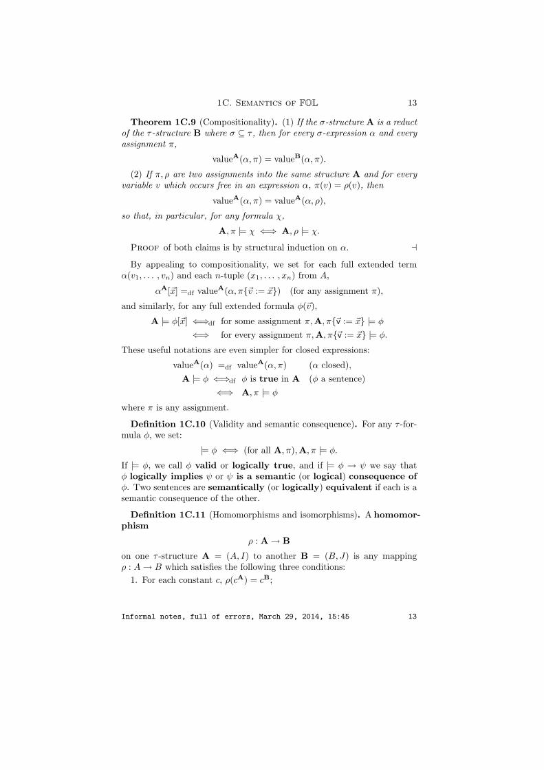
Theorem 1C.9 (Compositionality). (1) If the σ-structure A is a reductof the τ -structure B where σ ⊆ τ , then for every σ-expression α and everyassignment π,
valueA(α, π) = valueB(α, π).
(2) If π, ρ are two assignments into the same structure A and for everyvariable v which occurs free in an expression α, π(v) = ρ(v), then
valueA(α, π) = valueA(α, ρ),
so that, in particular, for any formula χ,
A, π |= χ ⇐⇒ A, ρ |= χ.
Proof of both claims is by structural induction on α. aBy appealing to compositionality, we set for each full extended term
α(v1, . . . , vn) and each n-tuple (x1, . . . , xn) from A,
αA[~x] =df valueA(α, π~v := ~x) (for any assignment π),
and similarly, for any full extended formula φ(~v),
A |= φ[~x] ⇐⇒df for some assignment π,A, π~v := ~x |= φ
⇐⇒ for every assignment π,A, π~v := ~x |= φ.
These useful notations are even simpler for closed expressions:
valueA(α) =df valueA(α, π) (α closed),A |= φ ⇐⇒df φ is true in A (φ a sentence)
⇐⇒ A, π |= φ
where π is any assignment.
Definition 1C.10 (Validity and semantic consequence). For any τ -for-mula φ, we set:
|= φ ⇐⇒ (for all A, π),A, π |= φ.
If |= φ, we call φ valid or logically true, and if |= φ → ψ we say thatφ logically implies ψ or ψ is a semantic (or logical) consequence ofφ. Two sentences are semantically (or logically) equivalent if each is asemantic consequence of the other.
Definition 1C.11 (Homomorphisms and isomorphisms). A homomor-phism
ρ : A → B
on one τ -structure A = (A, I) to another B = (B, J) is any mappingρ : A → B which satisfies the following three conditions:
1. For each constant c, ρ(cA) = cB;
Informal notes, full of errors, March 29, 2014, 15:45 13

14 1. First order logic
2. for each n-ary function symbol f and all x1, . . . , xn ∈ A,
ρ(fA(x1, . . . , xn)) = fB(ρ(x1), . . . , ρ(xn));
3. for each n-ary relation symbol R and all x1, . . . , xn ∈ A,
RA(x1, . . . , xn)=⇒RB(ρ(x1, ), . . . , ρ(xn)).(1C-1)
It is a strong homomorphism if it also satisfies
RA(x1, . . . , xn) ⇐⇒ RB(ρ(x1, ), . . . , ρ(xn)),(1C-2)
which is stronger than (1C-1).
An embedding ρ : A ½ B is an injective strong homomorphism, and anisomorphism ρ : A½→B is an embedding which is bijective (one-to-oneand onto). We set
A ' B ⇐⇒ there exists an isomorphism ρ : A½→B,
and when these conditions hold, we say that A and B are isomorphic.
An isomorphism ρ : A½→A of a structure A onto itself is an automor-phism of A, and a structure A is rigid if it has no automorphisms otherthan the (trivial) identity function id : A ½→A,
id(x) = x.
The basic properties of homomorphisms in the next proposition are quiteeasy and we will leave the proof for Problem x1.4; here ρ π : V → B isthe composition of given π : V → A and ρ : A → B,
(ρ π)(v) = ρ(π(v)).
Proposition 1C.12. (a) If ρ : A → B is a homomorphism, then forevery term t and every assignment π into A,
valueB(t, ρ π) = ρ(valueA(t, π)).
(b) If ρ : A→→B is a surjective, strong homomorphism, then for everyformula φ of FOL−(τ) and every assignment π into A,
A, π |= φ ⇐⇒ B, ρ π |= φ,(1C-3)
so that, in particular, for every FOL−(τ)-sentence χ,
A |= χ ⇐⇒ B |= χ.(1C-4)
(c) If ρ : A½→B is an isomorphism, then (1C-3) holds for all FOL(τ)-formulas φ, and (1C-4) holds for all FOL(τ)-sentences χ.
Informal notes, full of errors, March 29, 2014, 15:45 14

1D. First order definability 15
1D. First order definability
A proposition Φ of ordinary (mathematical) English, about a certain τ -structure A is expressed by a sentence φ of FOL(τ) if Φ and φ “mean” thesame thing; similarly, a proposition Φ(x) about an arbitrary object x in astructure A is expressed by a formula φ(x) with one free variable x, if foreach x ∈ A, Φ(x) and φ(x) “mean” the same thing. For example,
(∀x)[x + 0 = x] means “every number added to 0 yields itself”.
We cannot make this notion of “expressing” precise unless we first definemeaning rigorously for both natural language and FOL. On the otherhand, we have a clear, intuitive understanding of it which is important forapplications: roughly speaking, φ expresses Φ if we can construct the firstfrom the second by straightforward translation, more-or-less word for word,“and”, “but”, “also” going to & , “all”, “each”, “any” going to ∀, etc. Forexample, “every number is either odd or even” refers to the structure ofarithmetic and translates to something of the form
(∀x)[φ(x) ∨ ψ(x)]
where φ(x) and ψ(x) can be constructed to express the properties of beingodd or even.
As it turns out, all mathematical propositions and properties can beexpressed by FOL(τ)-sentences or formulas on appropriate structures. Thisis one of the main discoveries of modern mathematical logic and the sourceof its applications to mathematics. We will explain how it works in thesequel, starting in this section with the theory of first order definability ona fixed structure.
Definition 1D.1 (The basic local notions). Suppose A is a τ -structure.An n-ary relation R ⊆ An on A is first order definable or elementary
on A, if there is a full extended formula χ(v1, . . . , vn) such that
R(~x) ⇐⇒ A |= χ[~x] (~x ∈ An).
A function f : An → A is A-explicit if for some full extended term α(~v)
f(~x) = αA[~x] (~x ∈ An).
A function f : An → A is first order definable or elementary on Aif its graph
Gf (~x,w) ⇐⇒ f(~x) = w
is elementary on A, i.e., if there is a full extended formula χ(~v, u) such that
f(~x) = w ⇐⇒ A |= χ[~x,w].
The elementary functions and relations of the standard structure N ofarithmetic are called arithmetical.
Informal notes, full of errors, March 29, 2014, 15:45 15

16 1. First order logic
The next theorem is useful, as it often frees us from needing to worryexcessively about the formal syntax of FOL.
Theorem 1D.2. The collection E(A) of A-elementary functions andrelations on the universe of a structure
A = (A, cAc∈Const, RAR∈Rel, fAf∈Funct)
has the following properties:(1) Each primitive relation RA is A-elementary; and the (binary) identity
relation x = y is A-elementary.(2) For each constant symbol c and each n, the n-ary constant function
g(~x) = cA
is A-elementary; each primitive function fA is A-elementary; andevery projection function
Pni (x1, . . . , xn) = xi (1 ≤ i ≤ n)
is A-elementary.(3) E(A) is closed under substitutions of A-elementary functions: i.e., if
h(u1, . . . , um) is an m-ary A-elementary function and g1(~x), . . . , gm(~x)are n-ary, A-elementary, then the function
f(~x) = h(g1(~x), . . . , gm(~x))
is A-elementary; and if P (u1, . . . , um) is an m-ary A-elementary re-lation, then the n-ary relation
Q(~x) ⇐⇒ P (g1(~x), . . . , gm(~x))
is A-elementary.(4) E(A) is closed under the propositional operations: i.e., if P1(~x) and
P2(~x) are A-elementary, n-ary relations, then so are the followingrelations:
Q1(~x) ⇐⇒ ¬P1(~x),Q2(~x) ⇐⇒ P1(~x) & P2(~x),Q3(~x) ⇐⇒ P1(~x) ∨ P2(~x),Q4(~x) ⇐⇒ P1(~x) → P2(~x).
(5) E(A) is closed under quantification on A, i.e., if P (~x, y) is A-elementary,then so are the relations
Q1(~x) ⇐⇒ (∃y)P (~x, y),Q2(~x) ⇐⇒ (∀y)P (~x, y).
Moreover: E(A) is the smallest collection of functions and relations onA which satisfies (1) – (5).
Informal notes, full of errors, March 29, 2014, 15:45 16

1E. Arithmetical functions and relations 17
Proof. To show that E(A) has these properties, we need to constructlots of formulas and appeal repeatedly to the definition of A-elementaryfunctions and relations; this is tedious, but not difficult.
For the second (“moreover”) claim, we first make it precise by replacingE(A) by F throughout (1) – (5), and (temporarily) calling a class F offunctions and relations good if it satisfies all these conditions—so what hasalready been shown is that E(A) is good. The additional claim is that everygood F contains all A-elementary functions and relations, and it is verifiedby structural induction on the formula χ such that some full extension ofit χ(~v) defines a given, A-elementary relation—after showing, easily, thatthe graph of every A-explicit function is in F . a
The theorem suggests that E(A) is a very rich class of relations andfunctions. As it turns out, this is true for “rich”, “standard” structureslike N, but not true for structures with simple primitives—e.g., the plain(A) which has no primitives. We consider examples of these two kinds ofstructures in the next two sections.
1E. Arithmetical functions and relations
Is the exponential function
exp(t, x) = xt (x, t ∈ N)
arithmetical? Not obviously—but it is, as a corollary of a basic result aboutdefinition by recursion in N which we will prove in this section, and whichhas many important applications.
Definition 1E.1 (Primitive recursion). A function f : N→ N is definedby primitive recursion from the number w0 ∈ N and the binary functionh(w, t) if it satisfies the following two equations, for all t:
f(0) = w0, f(t + 1) = h(f(t), t);(1E-5)
more generally, a function f : Nn+1 → N of n+1 arguments on the naturalnumbers is defined by primitive recursion from the n-ary function g andthe (n + 2)-ary function h if it satisfies the following two equations, for allt, ~x:
f(0, ~x) = g(~x), f(t + 1, ~x) = h(f(t, ~x), t, ~x).(1E-6)
For example, if we set
f(0, x) = x, f(t + 1, x) = S(f(t, x)),
then (easily, by induction on t)
f(t, x) = t + x,
Informal notes, full of errors, March 29, 2014, 15:45 17

18 1. First order logic
and so addition is defined by primitive recursion from the two, simplerfunctions
g(x) = x, h(w, t, x) = S(w),
i.e., (essentially) the identity and the successor. Similarly, if we set
f(0, x) = 0, f(t + 1, x) = f(t, x) + x,
then, easily, f(t, x) = t · x, and so multiplication is defined by primitiverecursion from the functions
g(x) = 0, h(w, t, x) = w + t,
i.e., (essentially) the constant 0 and addition. More significantly (for ourpurposes here),
exp(0, x) = x0 = 1, exp(t + 1, x) = xt+1 = xt · x = exp(t, x) · x,
so that exponentiation is defined by primitive recursion from the functions
g(x) = 1, h(w, t, x) = w · x,
i.e., (essentially) the constant 1 and multiplication.
Theorem 1E.2. If f : Nn+1 → N is defined by the primitive recur-sion (1E-6) above and g, h are arithmetical, then so is f .
To prove this we must reduce the recursive definition of f into an explicitone, and this is done using Dedekind’s analysis of recursion:
Proposition 1E.3. If f : Nn+1 → N is defined by the primitive recur-sion in (1E-6), then for all t, ~x, w,
(1E-7) f(t, ~x) = w ⇐⇒ there exists a sequence (w0, . . . , wt) such that
w0 = g(~x) & (∀s < t)[ws+1 = h(ws, s, ~x)] & w = wt.
Proof. If f(t, ~x) = w, set ws = f(s, ~x) for s ≤ t, and verify easily thatthe sequence (w0, . . . , wt) satisfies the conditions on the right. For theconverse, suppose that (w0, . . . , wt) satisfies the conditions on the rightand prove by (finite) induction on s ≤ t that ws = f(s, ~x). a
We can view the equivalence (1E-7) as a theorem about recursive defini-tions which have already been justified in some other way; or we can see itas a definition of a function f which satisfies the recursive equations (1E-6)and so justifies recursive definitions—which is how Dedekind saw it. In anycase, it reduces proving Theorem 1E.2 to justifying quantification over fi-nite sequences within the class of arithmetical relations, and we will do thisby an arithmetical coding of finite sequences whose construction requires acouple of basic facts from arithmetic.
Informal notes, full of errors, March 29, 2014, 15:45 18

1E. Arithmetical functions and relations 19
Proposition 1E.4 (The Division Theorem). For every natural numbery > 0 and every x ∈ N, there exist exactly one q and one r such that
x = y · q + r and 0 ≤ r < y.(1E-8)
This is verified easily by induction on x. If (1E-8) holds, we set
quot(x, y) = q, rem(x, y) = r,
and for completeness, we also let quot(x, 0) = 0, rem(x, 0) = x.
Theorem 1E.5 (The Chinese Remainder Theorem). If d0, . . . , dt arerelatively prime numbers and w0 < d0, . . . , wt < dt, then there exists somenumber a such that
w0 = rem(a, d0), . . . , wt = rem(a, dt).
Proof. Consider the set D of all (t + 1)-tuples bounded by the givennumbers d0, . . . , dt,
D = (w0, . . . , wt) | w0 < d0, . . . , wt < dt,which has |D| = d0d1 · · · dt members, and let
A = a | a < |D|which is equinumerous with D. Define the function π : A → D by
π(a) = (rem(a, d0), rem(a, d1), . . . , rem(a, dt)).
Now π is injective (one-to-one), because if f(a) = f(b) with a < b < |D|,then b − a is divisible by each of d0, . . . , dt and hence by their product D(which is what their being relatively prime implies); hence d ≤ b−a, whichis absurd since a < b < |D|. We now apply the Pigeonhole Principle: sinceA and D are equinumerous and π : A ½ D is an injection, it must be asurjection, and hence whatever (w0, . . . , wt) may be, there is an a < d suchthat
π(a) = (rem(a, d0), rem(a, d1), . . . , rem(a, dt)) = (w0, . . . , wt). aThe idea now is to code an arbitrary tuple (w0, . . . , wt) by a pair of
numbers (d, a), where d can be used to produce uniformly t + 1 relativelyprime numbers d0, . . . , dt and then a comes from the Chinese RemainderTheorem.
Lemma 1E.6 (Godel’s β-function). Set
β(a, d, i) = rem(a, 1 + (i + 1)d).
This is an arithmetical function, and for each sequence of numbers w0, . . . , wt
there exist numbers a and d such that
β(a, d, 0) = w0, . . . , β(a, d, t) = wt.
Informal notes, full of errors, March 29, 2014, 15:45 19

20 1. First order logic
Proof. The β-function is arithmetical because it is defined by substi-tutions from addition, multiplication and the remainder function, which isarithmetical since
rem(x, y) = r ⇐⇒ (∃q)[x = yq + r & r < y].
To find the required a, d which code the tuple (w0, . . . , wt), set
s = max(t + 1, w0, . . . , wt), d = s!
and verify that the t + 1 numbers
d0 = 1 + (0 + 1)d, d1 = 1 + (1 + 1)d, . . . , dt = 1 + (t + 1)d
are relatively prime. (If a prime p divides 1+(1+ i)s! and also 1+(1+ j)s!with i < j, then it must divide their difference (j − i)s!, and hence it mustdivide one of (j− i) or s!; in either case, it divides s!, since (j− i) ≤ s, andthen it must divide 1, since it is assumed to divide 1 + (1 + i)s!, which isabsurd.) It is also immediate that wi < d = s!, by the definition of s, andso the Chinese Remainder Theorem supplies some a such that
(w0, . . . , wt) = (rem(a, d0), . . . , dt) = (β(a, d, 0), . . . , β(a, d, t))
as required. aProof of Theorem 1E.2. By the Dedekind analysis and using the β-
function to code tuples, we have
f(t, ~x) = w ⇐⇒ (∃a)(∃d)[β(a, d, 0) = g(~x)
& (∀s < t)[β(a, d, s + 1) = h(β(a, d, s), s, ~x)] & β(a, d, t) = w]
Thus the graph of f is arithmetical, by the closure properties of the arith-metical functions and relations in Theorem 1D.2. a
Remark. It may seem a little surprizing that we needed to use (for thefirst time) some number theory to prove Theorem 1E.2, but think aboutit: this is a result about the structure N = (N, 0, S, +, ·), not about anystructure in the vocabulary of arithmetic, which says something non-trivialabout “the natural numbers”, and it stands to reason that its proof mustuse something about them.
There is no single, standard definition of rich structure, but the followingnotion covers many important examples:
Definition 1E.7 (Structures with tuple coding). A copy of N in a struc-ture A is a structure N′ = (N′, 0′, S′, +′, ·′) such that:
1. N′ is isomorphic with the structure of arithmetic N.2. N′ ⊆ A.3. The set N′, the object 0′ and the functions S′, +′ and ·′ are all A-
elementary.
Informal notes, full of errors, March 29, 2014, 15:45 20

1E. Arithmetical functions and relations 21
A structure A admits tuple coding if it has a copy of N and there is anA-elementary function γ : An+1 → A such that for every tuple w0, . . . , wt ∈A, there is some ~a ∈ An such that
γ(~a, 0) = w0, γ(~a, 1) = w1, . . . , γ(~a, t) = wt,
where 0, 1, . . . , t are the “A-numbers” 0, 1, . . . , t (i.e., the copies of thesenumbers into A by the given isomorphism of N with N′).
In this definition, γ plays the role of the β-function in N, and we haveallowed for the possibility that triples (n = 3) or quadruples (n = 4) areneeded to code tuples of arbitrary length in A using γ. We might havealso allowed the natural numbers to be coded by pairs of elements of A ortweak the definition in various other ways, but this version captures all theinteresting examples already. The key result is:
Proposition 1E.8. Suppose A admits coding of tuples,
g : An → A, h : An+2 → A;
are A-elementary, f : An+1 → A, and for t ∈ N ′, y /∈ N ′,
f(0, ~x) = g(~x), f(t + 1, ~x) = h(f(t, ~x), t, ~x)), f(y, ~x) = y;(1E-9)
it follows that f is A-elementary.
It can be used to show that structures which admit tuple coding have arich class of elementary functions and relations.
Example 1E.9 (The integers). The ring of (rational) integers
Z = (Z, 0, 1, +, ·) (Z = . . . ,−2,−1, 0, 1, 2, . . . )(1E-10)
admits tuple coding.To see this, we use the fact that N ⊆ Z, and it is a Z-elementary set
because of Lagrange’s Theorem, by which every natural number is the sumof four squares:
x ∈ N ⇐⇒ (∃u, v, s, t)[x = u2 + v2 + s2 + t2] (x ∈ Z).
We can then use the β-function (with some tweaking) to code tuples ofintegers.
Example 1E.10 (The fractions). The field of rational numbers (frac-tions)
Q = (Q, 0, 1, +, ·)admits tuple coding.
This is a classical theorem of Julia Robinson which depends on a non-trivial, Q-elementary definition of N within Q.
Informal notes, full of errors, March 29, 2014, 15:45 21

22 1. First order logic
Example 1E.11 (The real numbers, with Z). The structure of analy-sis
(R,Z) = (R, 0, 1,Z,+, ·)admits tuple coding.
This requires some work—and it is not a luxury that we have includedthe integers as a distinguished subset: the field of real numbers
R = (R, 0, 1,+, ·)does not admit tuple coding. We will discuss this very interesting, classicalstructure later.
1F. Quantifier elimination
At the other end of the class of structures which admit tuple codingare some important, classical structures which are, in some sense, very“simple”: the elementary functions and relations on them are quite triv-ial. We will consider some examples of such structures in this section, andwe will isolate the property of quantifier elimination which makes them“simple”—much as tuple coding makes the structures in the preceding sec-tion complex.
We list first, for reference, some simple logical equivalences which we willbe using, and to simplify notation, we set for arbitrary τ -formulas φ, ψ andany τ -structure A:
φ ³A ψ ⇐⇒ A |= φ ↔ ψ,
φ ³ ψ ⇐⇒ |= φ ↔ ψ.
Proposition 1F.1 (Basic logical equivalences).(1) The distributive laws:
φ & (ψ ∨ χ) ³ (φ & ψ) ∨ (φ & χ), φ ∨ (ψ & χ) ³ (φ ∨ ψ) & (φ ∨ χ)
(2) De Morgan’s laws:
¬(φ & ψ) ³ ¬φ ∨ ¬ψ, ¬(φ ∨ ψ) ³ ¬φ & ¬ψ
(3) Double negation, implication and the universal quantifier:
¬¬φ ³ φ, φ → ψ ³ ¬φ ∨ ψ, ∀xφ ³ ¬(∃x)¬φ
(4) Renaming of bound variables: if y is a variable which does not occurin φ and φx :≡ y is the result of replacing x by y in all its free occurrences,then
∃xφ ³ ∃yφx :≡ y, ∀xφ ³ ∀yφx :≡ y
Informal notes, full of errors, March 29, 2014, 15:45 22

1F. Quantifier elimination 23
(5) Distribution law for ∃ over ∨:
∃x(φ1 ∨ · · · ∨ φn) ³ ∃xφ1 ∨ · · · ∨ ∃xφn
(6) Pulling the quantifiers to the front: if x does not occur free in ψ, then
∃xφ & ψ ³ ∃x(φ & ψ), ∃xφ ∨ ψ ³ ∃x(φ ∨ ψ)
∀xφ & ψ ³ ∀x(φ & ψ), ∀xφ ∨ ψ ³ ∀x(φ ∨ ψ)
∀xφ → ψ ³ ∃x[φ → ψ], ∃xφ → ψ ³ ∀x[φ → ψ]
(7) The general distributive laws: for all natural numbers n, k and everydoubly-indexed sequence of formulas φi,j with i ≤ n, j ≤ k,
∧∧i≤n
∨∨j≤k φi,j ³
∨∨f :0,... ,n→0,... ,k
∧∧i≤n φi,f(i).(1F-11)
∨∨i≤n
∧∧j≤k φi,j ³
∧∧f :0,... ,n→0,... ,k
∨∨i≤n φi,f(i).(1F-12)
Proof. To see (1F-11), fix a structure A and an assignment π andcompute:
A, π |= ∧∧i≤n
∨∨j≤k φi,j
⇐⇒ for each i ≤ n, there is some j ≤ k such that A, π |= φi,j
⇐⇒ there is a function f : 0, . . . , n → 0, . . . , ksuch that for all i ≤ n,A, π |= φi,f(i),
where (in the implication from left to right) the function f in the lastequivalence assigns to each i ≤ n the least j = f(i) ≤ k such that A, π |=φi,j . The dual (1F-12) is established by taking the negation of both sidesof (1F-11) applied to ¬φi,j , pushing the negation through the conjunctionsand disjunctions using De Morgan’s laws and finally applying the obvious¬¬φi,j ³ φi,j . a
1F.2 (Literals). For the constructions in the remainder of this section,it is useful to enrich the language FOL(τ) with propositional constants t, ffor truth and falsity. We may think of these as abbreviations,
t :≡ ∃x(x = x), f :≡ ∀x(x 6= x),
considered (by convention) as prime formulas. A literal is either t or f ora prime formula R(t1, . . . , tn), s = t or the negation of a prime formula:
` :≡ t | f | R(t1, . . . , tn) | s = t | ¬R(t1, . . . , tn) | ¬s = t
Proposition 1F.3 (Disjunctive normal form). Every quantifier-free for-mula χ is (effectively) logically equivalent to a disjunction of conjunctionsof literals which has no variables that do not occur in χ: i.e., for suitablen, ni, and literals `ij (i = 1, . . . , n, j = 1, . . . , ni) whose variables all occurin χ,
χ ³ χ∗ ≡ φ1 ∨ · · · ∨ φn, where for i = 1, . . . , n, φi ³ `i1 & · · · & `ini .
Informal notes, full of errors, March 29, 2014, 15:45 23

24 1. First order logic
By the definition in the proposition, x = y∨¬(z = z) is not a disjunctivenormal form of x = y (if all three variables are distinct), even though
x = y ³ x = y ∨ ¬(z = z)
Proof. We show by structural induction that for every quantifier-freeformula χ, both χ and its negation ¬χ are logically equivalent to a dis-junction of conjunctions of literals, among which we count t (truth) and f(falsity).
The result is trivial in the Basis, when χ is prime, since χ and ¬χ are indisjunctive normal form with n = 1, n1 = 1, and `11 ≡ χ or `11 ≡ ¬χ.
In the Induction Step, the proposition is immediate for χ ≡ ¬χ1, sincethe Induction Hypothesis gives us disjunctive normal form for χ1 ³ ¬χ and¬χ1 ≡ χ.
If χ is a disjunction or conjunction of χ1 and χ2, we may assume thatthe disjunctive normal forms for χ1 and χ2
χ1 ³∨∨
i<n
∧∧j<k χ1,i,j , χ2 ³
∨∨i<n
∧∧j<k χ2,i,j
given by the induction hypothesis have the same number of disjuncts andconjuncts, by “padding”—adding harmless insertions of t and f. We getimmediately a disjunctive normal form for the disjunction:
χ1 ∨ χ2 ³( ∨∨
i<n
∧∧j<k χ1,i,j
)∨
( ∨∨i<n
∧∧j<k χ2,i,j
)
³ ∨∨i<2n
[either i < n and
∧∧j<k χ1,i,j or n ≤ i and
∧∧j<k χ1,i−n,j
]
³ ∨∨i<2n
∧∧j<k χ2,i,j
where
χi,j ≡
χ1,i,j , if i < n,
χ2,i−n,j , otherwise.
To get a disjunctive normal form for the conjunction χ1 & χ2, we use thedistributive laws (1F-11), (1F-12) which give us equivalent conjunctive nor-mal forms
χ1 ³∧∧
i<n
∨∨j<k χ1,i,j , χ2 ³
∧∧i<n
∨∨j<k χ2,i,j
for the conjuncts, and using these we compute as above:
χ1 & χ2 ³( ∧∧
i<n
∨∨j<k χ1,i,j
)&
( ∧∧i<n
∨∨j<k χ2,i,j
)³ ∧∧
i<2n
∨∨j<k χi,j
where
χi,j ≡
χ1,i,j , if i < n,
χ2,i−n,j , otherwise.
We now use (1F-11) again to get a disjunctive normal form for χ1 & χ2.
Informal notes, full of errors, March 29, 2014, 15:45 24

1F. Quantifier elimination 25
These two computations also give us disjunctive normal forms for thenegations of disjunction and conjunctions by appealing to the De MorganLaws, and also for implication, using χ1 → χ2 ³ ¬χ1 ∨ χ2. a
Proposition 1F.4 (Prenex normal forms). Every formula χ is (effec-tively) logically equivalent to a formula
χ∗ ≡ Q1x1 · · ·Qnxnψ (ψ quantifier-free)
in prenex form, whose free variables are among the free variables of χ.
Definition 1F.5 (Quantifier elimination for structures). A quantifier-free normal form for a formula χ in a structure A is any quantifier-freeformula χ∗ (in which t or f may appear) whose variables are among thefree variables of χ and such that
χ ³A χ∗.
A structure A admits elimination of quantifiers, if every formula χhas a quantifier-free normal form in A; and it admits effective elimina-tion of quantifiers, if there is an effective procedure which will computefor each χ a quantifier-free normal form for χ in A.
1F.6. Quantifier elimination and decidability. To see the impor-tance of this notion, suppose the vocabulary τ is purely relational, i.e., ithas no constant or function symbols. Now the only quantifier-free sentencesare t and f; and so if a τ -structure A admits effective quantifier elimination,then we can effectively decide for each sentence χ whether it is logicallyequivalent in A to t or f—in other words, we have a decision procedurefor truth in A.
More generally, suppose τ may have constants and function symbols andA admits effective quantifier elimination: if we have a decision procedurefor quantifier-free sentences (with no variables), then we have a decisionprocedure for truth in A. The hypothesis is, in fact, satisfied by manystructures that occur naturally in mathematics, including (trivially) thestructure of arithmetic N = (N, 0, 1, +, ·); so we cannot expect that Nadmits effective quantifier elimination, because we don’t expect it to bedecidable—and in time we will prove that it is not decidable.
Lemma 1F.7 (Quantifier elimination test). If every formula of the form
χ ≡ ∃x[χ1 & · · · & χn] (where χ1, . . . , χn are literals)
is (effectively) equivalent in a structure A to a quantifier-free formula whosevariables are all among the free variables of χ, then A admits (effective)quantifier elimination.
Proof. Let F be the set of formulas which (effectively) have quantifierfree forms in A. It is enough to show that F contains all literals, which it
Informal notes, full of errors, March 29, 2014, 15:45 25

26 1. First order logic
clearly does; that it is closed under ¬, & and ∨, which it clearly is; andthat it is closed under ∃, which then implies that it is also closed under ∀by (3) of Proposition 1F.1. For the last of these, if
χ ≡ ∃xφ
with φ quantifier-free, we bring φ to disjunctive normal form, so that
χ ³ ∃x[φ1 ∨ · · · ∨ φn] ³ ∃xφ1 ∨ · · · ∨ ∃xφn
where each φi is a conjunction of literals and then we use the hypothesisof the Lemma. a
Proposition 1F.8. For each infinite set A, the structure A = (A) inthe language with empty vocabulary admits effective quantifier elimination.
Proof. By the Basic Test 1F.7, it is enough to eliminate the quantifierfrom every formula of the form
χ ³ ∃x[(x = z1 & · · · & x = zk) & (u1 = v1 & · · ·ul = vl)
& (x 6= w1 & · · · & x 6= wm) & (s1 6= t1 & · · · & to 6= so)]
where we have grouped the variable equations and inequations according towhether x occurs in them or not, i.e., x is none of the variables ui, vi, si, ti.We can also assume that x is none of the variables zi, since the equationx = x can simply be deleted; and it is none of the variables wi, since ifx 6= x is one of the conjuncts, then χ ³ F .
Case 1, k = 0, i.e., there is no equation of the form x = z in the matrixof χ. In this case
χ ³ (u1 = v1 & · · ·ul = vl) & (s1 6= t1 & · · · & tm 6= sm).
This is because if π is any assignment which satisfies
(u1 = v1 & · · ·ul = vl) & (s1 6= t1 & · · · & tm 6= sm)
and t is any element in the (infinite) set A which is distinct from π(w1), . . . ,π(wm), then πx := t satisfies the matrix of χ.
Case 2, k > 0, so there is an equation x = zi in the matrix of χ. In thiscase,
χ ³ (x = z1 & · · · & x = zk)x :≡ zi & (u1 = v1 & · · ·ul = vl)
& (x 6= w1 & · · · & x 6= wm)x :≡ zi & (s1 6= t1 & · · · & tm 6= sm)]
since every assignment which satisfies χ must assign to x the same valuethat it assigns to zi. a
This proposition is about a structure of no interest whatsoever, but themethod of proof is typical of many quantifier elimination proofs.
Informal notes, full of errors, March 29, 2014, 15:45 26

1F. Quantifier elimination 27
Definition 1F.9 (Dense linear orderings). A linear ordering L = (L,≤)is dense in itself if for every x, y ∈ L such that x < y, there is a z suchthat x < z < y.
Standard examples are the usual orderings (Q,≤) and (R,≤) on therational and the real numbers. They also have no least or greatest element,and so they are covered by the next result.
Theorem 1F.10. If L = (L,≤) is a dense linear ordering without leastor greatest element, then L admits effective quantifier elimination.
Proof. It is convenient to introduce a new symbol < for strict inequal-ity, so that
x ≤ y ³L x = y ∨ x < y, x < y ³L x ≤ y & x 6= y.(1F-13)
We can use the first of these equivalences to eliminate the symbol ≤,so that every formula is logically equivalent in L to one in which only thesymbols = and < occur. In particular, the literals which occur in disjunctivenormal forms of quantifier free formulas are all in one of the forms
x = y, x 6= y, x < y, ¬(x < y)
We now replace all the negated literals by quantifier free formulas whichhave no negation using the equivalences
x 6= y ³L x < y ∨ y < x, ¬(x < y) ³L x = y ∨ y < x,(1F-14)
and then we apply repeatedly the Distributive Laws in Proposition 1F.1(which do not introduce negations) to construct a disjunctive normal formwith only positive literals x = y and x < y. This means that in applyingthe basic test Lemma 1F.7, we need consider only formulas of the form
χ ≡ ∃x[(x = z1 & · · · & x = zk)
& (x < u1 & · · · & x < ul) & (v1 < x & · · · & vm < x)
& (s1 < s′1 & · · · & sn < s′n) & (t1 = t′1 & · · · & to = t′o)]
If some ui ≡ x of some vj ≡ x, then χ ³L f, so we may assume thatthese variables are all distinct from x.
Case 1, k > 0, so that some equation x = zi is present in the matrix.Now χ is equivalent to the quantifier-free formula which is constructed byreplacing x by zi in the matrix.
Case 2, k = l = m = 0, so that x does not occur in the matrix of χ. Wesimply delete the quantifier.
Case 3, k = l = 0 but m > 0. In this case
χ ³L (s1 < s′1 & · · · & sn < s′n) & (t1 = t′1 & · · · & to = t′o)]
Informal notes, full of errors, March 29, 2014, 15:45 27

28 1. First order logic
because whatever values are assigned to v1, . . . , vm by an assignment, somegreater value can be assigned to x since L has no largest element.
Case 4, k = m = 0 but l > 0. This case is symmetric to Case 3, and wehandle it using the fact that L has no least element.
Case 5, k = 0 but m > 0, l > 0. Since L is dense in itself, the restrictionson x in the matrix will be satisfied by some x exactly when
maxv1, . . . , vm < minu1, . . . , ul,and we can say this formally by a big conjunction: i.e.,
χ ³L
∧∧1≤i≤l,1≤j≤m(vj < ui)
& (s1 < s′1 & · · · & sn < s′n) & (t1 = t′1 & · · · & to = t′o)
This completes the verification of the test, Lemma 1F.7 for dense linearorderings with no first and last element, and so these structures admiteffective quantifier elimination. a
There are many interesting structures which admit effective quantifierelimination, including the following:
Example 1F.11. The reduct (N, 0, S) of N without addition or mul-tiplication admits effective quantifier elimination, as does the somewhatricher structure (N, 0, S, <).
Example 1F.12 (Presburger arithmetic). The reduct (N, 0, S,+) of Ndoes not quite admit quantifier elimination, but something quite close toit does. Let
x ≡m y ⇐⇒ m divides y − x (x is congruent to y mod m),
and consider the expansion of (N, 0, S, +) by these infinitely many relations,
NP = (N, 0, S, +, ≡mm∈N).
This structure admits effective quantifier elimination and there is a trivialdecision procedure for quantifier free sentences, which involve only numeralsand congruence assertions about them; and so it is a decidable structure,and then the structure (N, 0, S, +) of additive arithmetic is also decidable,since it is a reduct of NP .
This is a famous and not so simple theorem of Presburger, Theorem 32Ein A mathematical introduction to logic, Second Edition by HerbertB. Enderton.
Note that the expansion of the language by these congruence relations isquite similar to the expansion with t and f which we have assumed as partof the definition of “quantifier elimination”, because it is so often needed.
Informal notes, full of errors, March 29, 2014, 15:45 28

1G. Theories and elementary classes 29
The congruence relations are simply definable in additive arithmetic, one-at-a-time:
x ≡m y :≡ (∃z)[(x + z + z + · · ·+ z︸ ︷︷ ︸m times
= y) ∨ (y + z + z + · · ·+ z︸ ︷︷ ︸m times
= x)].
The quantifier elimination in Presburger’s structure NP yields for eachχ a quantifier-free formula in which these new, prime formulas x ≡m yoccur, for various values of m; we can then replace all of them with theirdefinition, which gives us a formula χ∗ which is ³NP
with χ and in whichexistential quantifiers occur only in the “literals”. This is exactly the sortof “extended quantifier-free” formulas that we will get if we replace t andf by their definitions after the quantifier elimination procedure has beencompleted.
Example 1F.13 (The field of complex numbers). The field of complexnumbers
C = (C, 0, 1, +, ·)admits effective quantifier elimination, and so it is decidable, since thequantifier-free sentences in the language involve only trivial equalities andinequalities about numerals. (We will later give a model-theoretic proof ofthis basic fact.)
Example 1F.14 (The ordered field of real numbers). The structure
Ro = (R, 0, 1,+, ·,≤)
admits effective quantifier elimination, and so it is decidable, as above.This is a famous theorem of Tarski, especially important because it es-
tablishes the decidability of classical (ancient) Euclidean plane and spacegeometry: it is easy to see that if we use Cartesian coordinates, we cantranslate all the elementary propositions studied in Euclidean geometryinto sentences in the language of Ro, and then decide them by Tarski’salgorithm. Contrast this result with Example 1E.11: if we just add a namefor the set of integers Z to the language, we get a structure which admitstuple coding, in whose language we can formalize all the propositions ofclassical analysis—including calculus.
The hint to Problem x1.29∗ suggests a proof of the simpler fact, that thelinear reduct (R, 0, 1,+,≤) of Ro (without multiplication) admits effectivequantifier elimination.
1G. Theories and elementary classes
Next we consider how formal, FOL sentences can be used to define prop-erties of structures.
Informal notes, full of errors, March 29, 2014, 15:45 29

30 1. First order logic
Definition 1G.1 (Elementary classes of structures). A property Φ of τ -structures is basic elementary if there exists a sentence φ in FOL(τ) suchthat for every τ -structure A,
A has property Φ ⇐⇒ A |= φ,
and it is elementary if there exists a (possible infinite) set of sentences Tsuch that
A has property Φ ⇐⇒ for every φ ∈ T ,A |= φ.
Basic elementary properties of τ -structures are (obviously) elementary, butwe will shortly show that the converse is not always true.
Instead of a “property” of τ -structures, we often speak of a class (col-lection) of τ structures and formulate these conditions for classes, in theform
A ∈ Φ ⇐⇒ A |= φ (basic elementary class)A ∈ Φ ⇐⇒ for every φ ∈ T ,A |= φ (elementary class).
Notice that by Proposition 1C.12, basic elementary and elementary classesare closed under isomorphisms.
Definition 1G.2 (Theories and models). A (formal, axiomatic) theoryin a language FOL(τ) is any (possibly infinite) set of sentences T of FOL(τ).The members of T are its axioms.
A τ -structure A is a model of T if every sentence of T is true in A: wewrite
A |= T ⇐⇒df for all φ ∈ T, A |= φ,(1G-15)
and we collect all the models of T into a class,
Mod(T ) =df A | A |= T.(1G-16)
Notice that Mod(T ) is an elementary class of structures—and if T is finite,then Mod(T ) is a basic elementary class, axiomatized by the conjunctionof all the axioms in T .
In the opposite direction, the theory of a τ-structure A is the set ofall FOL(τ)-sentences that it satisfies,
Th(A) =df χ | χ is a sentence and A |= χ.(1G-17)
And finally,
T |= χ ⇐⇒ for every A, if A |= T, then A |= χ.(1G-18)
This is the fundamental notion of semantic consequence (from an arbi-trary set of hypotheses) for the language FOL.
Informal notes, full of errors, March 29, 2014, 15:45 30

1G. Theories and elementary classes 31
Remark. It is quite common in the literature to call a set of sentencesT a “theory” only if it closed under logical consequence, i.e., if
T |= χ=⇒χ ∈ T.
We have not done this here because we want to keep track of the specificaxioms we use; but it is advisable to check the definitions carefully if youread results about arbitrary theories in some book or paper.
One of the basic problems in logic is the relation between a structure Aand its theory Th(A): how much of A is captured by “all the first-orderfacts about A” collected in Th(A)?
Definition 1G.3 (Elementary equivalence). Two τ -structures are ele-mentarily equivalent if they satisfy the same FOL(τ)-sentences, in sym-bols
A ≡ B ⇐⇒df Th(A) = Th(B).(1G-19)
As an immediate consequence of Proposition 1C.12 we get:
Proposition 1G.4. Isomorphic structures are elementarily equivalent.
We will see later that (somewhat surprisingly) the converse of this Propo-sition does not hold.
Axiomatic theories are useful, because they allow us to prove propertiesof many, related structures simultaneously, for all of them, by deriving them“from the axioms”. We formulate here a few, basic theories we can use forexamples later on.
Definition 1G.5 (Graphs). The theory SG of symmetric graphs is for-mulated in the language FOL(E) with just one, binary relation symbol Eand one axiom,
∀x∀y[R(x, y) ↔ R(y, x)].
The symmetric graphs then are exactly the models of SG.
Definition 1G.6 (Theories of order). The theories of partial and linearorderings are also formulated in the language with vocabulary just one,binary relation symbol typically ≤:
PO =df ∀x(x ≤ x), ∀x∀y[(x ≤ y & y ≤ x) → x = y],∀x∀y∀z[(x ≤ y & y ≤ z) → x ≤ z]
LO =df PO ∪ ∀x∀y[x ≤ y ∨ y ≤ x]DLO =df LO ∪ ∀x∀y[x < y → ∃z(x < z & z < y)]
∀x∃y[x < y], ∀y∃x[x < y]
Informal notes, full of errors, March 29, 2014, 15:45 31

32 1. First order logic
The last of these is the theory of dense linear orderings without first andlast element, and we have shown that every model of DLO admits effectivequantifier elimination, Theorem 1F.10. The proof, actually, was uniform,and so it shows that the theory DLO admits effective quantifier elimination,in the following, precise sense.
Definition 1G.7 (Quantifier elimination for theories). A theory T in thelanguage FOL(τ) admits elimination of quantifiers, if for every τ -formula χ, there is a quantifier-free formula χ∗ (whose variables are allamong the free variables of χ) such that
T |= χ ↔ χ∗.
As with structures, we assume here that the language is expanded by theprime, propositional constants t and f which may occur in χ∗.
Corollary 1G.8. The theory DLO of dense linear orderings without firstor last element admits effective quantifier elimination, and so it is decid-able.
Proof follows immediately from the proof of Theorem 1F.10, whichproduces the same quantifier-free form L-equivalent to a given χ, indepen-dently of the specific L, just so long as L |= DLO.
The second claim simply means that we can decide for any given sentenceχ whether or not DLO |= χ. It is true because the quantifier eliminationprocedure yields either t or f as L-equivalent to χ, independently of thespecific L. a
Definition 1G.9 (Fields). The theory Fields comprises the formal ex-pressions of the axioms for a field listed in Definition 1A.4, in the languageFOL(0, 1,+, ·).
For each number n ≥ 1 define the term n · 1 by the recursion
1 · 1 ≡ 1, (n + 1) · 1 ≡ (n · 1) + (1),
so that e.g., 3 · 1 ≡ ((1)+ (1))+ (1). (Make sure you understand here whatis a term of FOL(0, 1,+, ·), what is an ordinary number, and which + ismeant in the various places.)
For each prime number p, the finite set of sentences
Fieldsp =df Fields, ¬(2 · 1 = 0), . . . ,¬((p− 1) · 1 = 0), p · 1 = 0
is the theory of fields of characteristic p. The theory of fields of character-istic 0 is defined by
Fields0 =df Fields, ¬(2 · 1 = 0), ¬(3 · 1 = 0), . . . .
In describing sets of formulas here we use “,” to indicate union, i.e., in setnotation,
Fields0 =df Fields ∪ ¬(2 · 1 = 0), ¬(3 · 1 = 0), . . . .
Informal notes, full of errors, March 29, 2014, 15:45 32

1G. Theories and elementary classes 33
The simplest example of a field of characteristic p is the finite structure
Zp = (0, 1, . . . , p− 1, 0, 1, +, ·)with the usual operations on it executed modulo p, but it takes some (al-gebra) work to show that this is a field. There are many other fields ofcharacteristic p, both finite and infinite.
The standard examples of fields of characteristic 0 are the rationals Q,the reals R and the complex numbers C.
For prime p, Fieldsp is a finite set of sentences, while Fields0 is infinite.
Definition 1G.10 (Peano Arithmetic, PA). The axioms of Peano arith-metic PA are the universal closures of the following formulas, in the lan-guage FOL(0, S, +, ·) of the structure of arithmetic (which we will call fromnow on the language of Peano arithmetic).
(1) ¬(S(x) = 0) &(S(x) = S(y) → x = y
).
(2) x + 0 = x, x + S(y) = S(x + y).(3) x · 0 = 0, x · (Sy) = x · y + x.(4) For every full extended formula φ(x, ~y),
[φ(0, ~y) & (∀x)[φ(x, ~y) → φ(S(x), ~y)]
]→ (∀x)φ(x, ~y).
The last of these is the (elementary) Induction Axiom Scheme whichapproximates in FOL the Induction Principle, (4) in Definition 1A.3. Ithas infinitely many instances, one for each full extended formula φ(x, ~y).
The standard (intended) model of PA is, of course, N, but we will seethat it has many others!
Definition 1G.11 (The Robinson system Q). This is a weak, finite the-ory of natural numbers in the language of Peano arithmetic, which replacesthe Induction Scheme by the single claim that every non-zero number is asuccessor:
1. ¬[S(x) = 0].2. S(x) = S(y) → x = y.3. x + 0 = x, x + (S(y) = S(x + y).4. x · 0 = 0, x · (Sy) = x · y + x.5. x = 0 ∨ (∃y)[x = S(y)].
It is clear that N is a model of Q, but Q is a weak theory, and so it is quiteeasy to construct many, peculiar models of it.
Definition 1G.12 (Axiomatic Set Theories). Of the nine (informal) ax-ioms of Zermelo-Fraenkel Set Theory listed in Definition 1A.5, all but (5)(Subsets) and (8) (Replacement) are easily expressible in the languageFOL(∈) of sets. As with Peano arithmetic, we can write down formalaxiom schemes which approximate those two, as follows:
Informal notes, full of errors, March 29, 2014, 15:45 33

34 1. First order logic
Axiom Scheme of Subsets: For each extended formula φ(u) in whichthe variable z does not occur free and u 6≡ x, the universal closure of thefollowing is an axiom:
(∃z)(∀u)[u ∈ z ↔ (u ∈ x & φ(u))].
Axiom Scheme of Replacement : For each extended formula φ(u, v) inwhich the variable z does not occur and x 6≡ u, v, the universal closure ofthe following is an axiom:
(∀u)(∃!v)φ(u, v) → (∃z)(∀v)[v ∈ z ↔ (∃u)[u ∈ x & φ(u, v)].
The theory ZC (Zermelo Set Theory with Choice) is the set of (formal)axioms (1) - (4), (6) - (7) and all the instances of the Axiom Scheme (5) ofSubsets.
The theory ZFC (Zermelo-Fraenkel Set Theory with Choice) is the set of(formal) axioms (1) - (4), (6) - (7), (9) and all the instances of the AxiomSchemes (5) of Subsets and (8) Replacement.
The theories Z and ZF are obtained from these by deleting the Axiom ofChoice (7).
1H. The Hilbert proof system for FOL
In this Section we will introduce formal FOL-proofs (from a theory T ),and in the next we will prove that they suffice to establish all semanticconsequences of T . This is the first fundamental result of logic.
1H.1. Axioms and rules of inference. The axioms (or axiomsschemes) and rules of inference of FOL(τ) are the following, subject tothe indicated restrictions; here φ, φ(v) etc. vary over arbitrary formulas orextended formulas.
Logical axioms.(1) φ → (ψ → φ)(2) (φ → ψ) → ((φ → (ψ → χ)) → (φ → χ))(3) (φ → ψ) → ((φ → ¬ψ) → ¬φ)(4) ¬¬φ → φ(5) φ → (ψ → (φ & ψ))
(6a) (φ & ψ) → φ (6b) (φ & ψ) → ψ(7a) φ → (φ ∨ ψ) (7b) ψ → (φ ∨ ψ)(8) (φ → χ) → ((ψ → χ) → ((φ ∨ ψ) → χ))(9) ∀vφ(v) → φ(t) (t free for v in φ(v)
(10) ∀v(φ → ψ) → (φ → ∀vψ) (v not free in φ)(11) φ(t) → ∃vφ(v) (t free for v in φ(v)
Informal notes, full of errors, March 29, 2014, 15:45 34

1H. The Hilbert proof system for FOL 35
Rules of inference:(12) φ, φ → ψ =⇒ψ (Modus Ponens)(13) φ=⇒∀vφ (Generalization)(14) φ → ψ =⇒∃vφ → ψ (v not free in ψ) (Exists elimination)
Axioms for identity. For every n-ary relation symbol R in τ and everyn-ary function symbol f in τ :(15) v = v, v = v′ → v′ = v, v = v′ → (v′ = v′′ → (v = v′′))(16) (v1 = w1 & . . . vn = wn) → (R(v1, . . . , vn) → R(w1, . . . , wn))
(R n-ary relation symbol)(17) (v1 = w1 & . . . vn = wn) → (f(v1, . . . , vn) = f(w1, . . . , wn))
(f n-ary function symbol)The Hilbert system for FOL− is obtained from this by allowing only
FOL−(τ)-formulas and omitting the axioms for identity. We will skip not-ing explicitly in the sequel these natural restrictions which must be madeto the definitions to get the right notions for FOL− from those for FOL,on which we will concentrate.
Definition 1H.2. A proof or deduction in FOL from a theory T isany sequence of formulas
φ0, φ1, . . . , φn,
where each φi is either an axiom, or a formula in T , or follows from previ-ously listed formulas by one of the rules of inference. We set
T ` φ ⇐⇒df there exists a deduction φ0, . . . , φn from T with φn ≡ φ.
If T = ∅ we just write ` φ.A deduction is propositional if the axioms 9-11 and the rules 13, 14 are
not used in it, and we write
T `prop φ ⇐⇒df there exists a propositional deduction of φ from T.
(The formulas in a propositional deduction may have quantifiers in them.)If T is a theory (a set of sentences) and T ` φ, we call φ a proof-theoretic
consequence or just a theorem of T . A propositional theorem of T isany formula φ for which there is a propositional deduction from T . Theproof-theoretic consequences of the empty theory are the theorems of FOL;the propositional theorems of FOL are called tautologies.
Lemma 1H.3. (1) If T ⊆ T ′, then every proof from T is also a prooffrom T ′.
(2) The concatenation
φ0, . . . , φn, ψ0, . . . , ψk
of two proofs from T is also a proof from T .
Informal notes, full of errors, March 29, 2014, 15:45 35

36 1. First order logic
(3) The set T = φ | T ` φ of theorems of T is the least set of formulaswhich contains T and all axioms and is closed under the inference rules(12), (13), (14).
Proof. (1) and (2) are trivial and they easily imply (3). aTheorem 1H.4 (Soundness). Every theorem of a theory T is a seman-
tic consequence of T , i.e.,
if T ` φ, then T |= φ.
Proof is immediate from (3) of the Lemma, since the set of semanticconsequences of T obviously contains T and all the axioms and is closedunder the inference rules. a
The main result in the next section is the converse of the SoundnessTheorem, which (in particular) identifies validity with provability. To proveit, we will obviously need to construct many formal proofs, and in this weare somewhat hampered by the definition of the Hilbert proof system whichis not very “user friendly”: it is not immediate how to construct formalproofs in it for even the simplest valid formulas. For example, the proof of(φ → φ) in the next lemma is about as simple as one can construct in theHilbert system—and it is not as simple as it should be:
Lemma 1H.5. For every formula φ, ` φ → φ.
Proof. For any φ and any φ′, the implication(φ → (φ′ → φ)
)→
[(φ → ((φ′ → φ) → φ)
)→ (φ → φ)
]
is an instance of Axiom Scheme (2) (with ψ ≡ (φ′ → φ)) and χ ≡ φ) andhence a tautology. Its hypothesis φ → (φ′ → φ) is an instance of AxiomScheme (1), and so by Modus Ponens, its conclusion
(φ → ((φ′ → φ) → φ)
)→ (φ → φ)
is also a tautology; but the hypothesis φ → ((φ′ → φ) → φ) of this isalso an instance of Axiom Scheme (1), and so its conclusion φ → φ is atautology. a
We will introduce later a more natural proof system which is more suit-able for “formalizing” ordinary mathematical proofs. It is simpler, however,to first prove the Completeness Theorem using this Hilbert system and theninfer it for more natural systems of proofs. We list here some preliminaryresults which we will need for this purpose, mostly skipping the proofswhich are quite easy.
Lemma 1H.6 (Constant Substitution). Suppose T is a theory, the vari-able v does not occur bound in the sequence of formulas φ1(v), . . . , φn(v)
Informal notes, full of errors, March 29, 2014, 15:45 36

1H. The Hilbert proof system for FOL 37
of FOL(τ) and c is a fresh constant, i.e., a constant which does not occurin T or any of the formulas φ1(v), . . . , φn(v); then
φ1(v), . . . , φn(v) is a deduction from T
⇐⇒ φ1(c), . . . , φn(c) is a deduction from T .
Proof. See Problem x1.37. aLemma 1H.7 (The Propositional Deduction Theorem). For every the-
ory T and all formulas χ, φ,
T, χ `prop φ ⇐⇒ T `prop χ → φ,
where the subscript indicates that the given and resulting deductions arepropositional.
Proof. For the direction (⇐) we have the proof from T, χ
(χ → φ), χ, φ.
The more interesting direction (⇒) is proved by induction on the length ofa given proof of φ from T, χ, cf. Problem x1.38 a
Theorem 1H.8 (The Deduction Theorem). For every theory T , everysentence χ and every formula φ,
T, χ ` φ ⇐⇒ T ` χ → φ.
We leave the proof for Problem x1.39.In the next two theorems we formulate some natural deduction rules
for the Hilbert system which help formalize in it ordinary mathematicalarguments. We will not need to appeal to these very much, but theyhelp explain how to formalize in the Hilbert system ordinary mathematicalarguments.
Theorem 1H.9 (The natural introduction rules). If T is a set of sen-tences, the indicated substitutions are free and the additional restrictionshold:
(→) If T, χ ` φ, then T ` χ → φ.Restriction: χ is a sentence.
(&) φ, ψ ` φ & ψ.(∨) φ ` φ ∨ ψ, ψ ` φ ∨ ψ.(¬) If T, χ ` ψ and T, χ ` ¬ψ, then T ` ¬χ (Proof by contradiction).
Restriction: χ is a sentence.(∀) φ ` ∀v′φv :≡ v′ (Generalization rule).(∃) φv :≡ t ` ∃vφ.
Theorem 1H.10 (The natural elimination rules). If T is a set of sen-tences, the indicated substitutions are free and the additional restrictionshold:
Informal notes, full of errors, March 29, 2014, 15:45 37

38 1. First order logic
(→) φ, φ → ψ ` ψ.(&) φ & ψ ` φ, φ & ψ ` ψ.(∨) If T, φ ` χ and T, ψ ` χ, then T, φ ∨ ψ ` χ (Proof by cases).
Restriction: φ, ψ must be sentences.(¬) ¬¬φ ` φ (Double negation elimination).(∀) ∀vφ ` φv :≡ t.(∃) If T, φ ` χ, then T, ∃vφ ` χ (∃-elimination rule).
Restriction: v does not occur free in χ, ∃vφ is a sentence, and thegiven proof has no bound occurrence of v.
We end the section with the definitions of three basic, proof-theoreticnotions about theories:
Definition 1H.11. Suppose T is a τ -theory:(1) T is consistent if it does not prove a contradiction, i.e., if there is no
χ such that T ` χ & ¬χ.(2) T is complete if for each τ -sentence θ, either T ` θ or T ` ¬θ.(3) A τ ′-theory T ′ is a conservative extension of T if τ ⊆ τ ′ and for
every τ -sentence θ,
T ` θ ⇐⇒ T ′ ` θ.
Lemma 1H.12. (1) A theory T is consistent if and only if there is somesentence χ such that T 0 χ.
(2) A theory T is consistent if and only if every finite subset T0 ⊆ T isconsistent.
(3) For any theory T and any sentence χ,
T ` χ ⇐⇒ T ∪ ¬χ is inconsistent.
(4) If T is consistent, then for every sentence χ, either T ∪ χ is con-sistent, or T ∪ ¬χ is consistent.
(5) If ∃vφ(v) is a sentence, T∪∃vφ(v) is consistent and c is a constantwhich does not occur in T or in ∃vφ(v), then T ∪ φ(c) is consistent.
We leave the (easy) proof for Problem x1.47.
1I. The Completeness Theorem
In this section we will prove the basic result of First Order Logic:
Theorem 1I.1 (Godel’s Completeness Theorem). (1) Every consistent,countable theory T has a countable model.
(2) For every countable τ -theory T and every τ -sentence χ,
if T |= χ, then T ` χ.(1I-20)
Informal notes, full of errors, March 29, 2014, 15:45 38
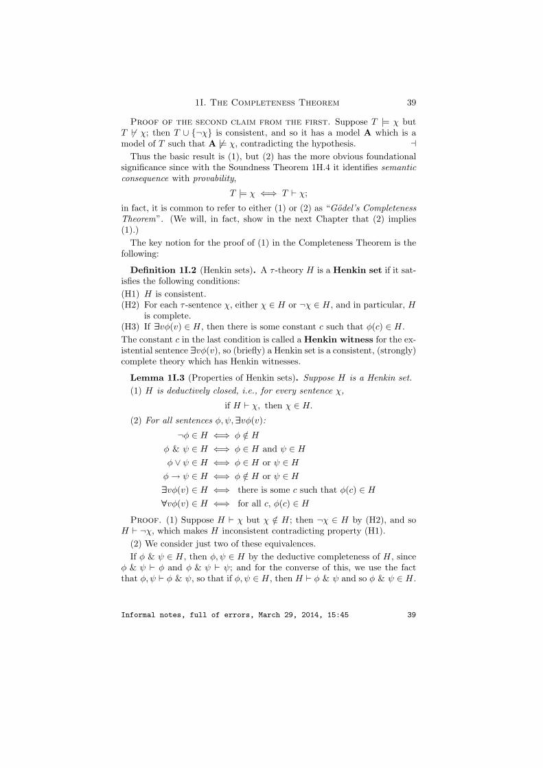
1I. The Completeness Theorem 39
Proof of the second claim from the first. Suppose T |= χ butT 6` χ; then T ∪ ¬χ is consistent, and so it has a model A which is amodel of T such that A 6|= χ, contradicting the hypothesis. a
Thus the basic result is (1), but (2) has the more obvious foundationalsignificance since with the Soundness Theorem 1H.4 it identifies semanticconsequence with provability,
T |= χ ⇐⇒ T ` χ;
in fact, it is common to refer to either (1) or (2) as “Godel’s CompletenessTheorem”. (We will, in fact, show in the next Chapter that (2) implies(1).)
The key notion for the proof of (1) in the Completeness Theorem is thefollowing:
Definition 1I.2 (Henkin sets). A τ -theory H is a Henkin set if it sat-isfies the following conditions:(H1) H is consistent.(H2) For each τ -sentence χ, either χ ∈ H or ¬χ ∈ H, and in particular, H
is complete.(H3) If ∃vφ(v) ∈ H, then there is some constant c such that φ(c) ∈ H.The constant c in the last condition is called a Henkin witness for the ex-istential sentence ∃vφ(v), so (briefly) a Henkin set is a consistent, (strongly)complete theory which has Henkin witnesses.
Lemma 1I.3 (Properties of Henkin sets). Suppose H is a Henkin set.(1) H is deductively closed, i.e., for every sentence χ,
if H ` χ, then χ ∈ H.
(2) For all sentences φ, ψ, ∃vφ(v):
¬φ ∈ H ⇐⇒ φ /∈ H
φ & ψ ∈ H ⇐⇒ φ ∈ H and ψ ∈ H
φ ∨ ψ ∈ H ⇐⇒ φ ∈ H or ψ ∈ H
φ → ψ ∈ H ⇐⇒ φ /∈ H or ψ ∈ H
∃vφ(v) ∈ H ⇐⇒ there is some c such that φ(c) ∈ H
∀vφ(v) ∈ H ⇐⇒ for all c, φ(c) ∈ H
Proof. (1) Suppose H ` χ but χ /∈ H; then ¬χ ∈ H by (H2), and soH ` ¬χ, which makes H inconsistent contradicting property (H1).
(2) We consider just two of these equivalences.If φ & ψ ∈ H, then φ, ψ ∈ H by the deductive completeness of H, since
φ & ψ ` φ and φ & ψ ` ψ; and for the converse of this, we use the factthat φ, ψ ` φ & ψ, so that if φ, ψ ∈ H, then H ` φ & ψ and so φ & ψ ∈ H.
Informal notes, full of errors, March 29, 2014, 15:45 39

40 1. First order logic
If ∃vφ(v) ∈ H, then φ(c) ∈ H for some c, by the key property (H3). Theconverse holds because φ(c) ` ∃vφ(v) and H is deductively complete. a
The lemma suggests that every Henkin set is Th(A) for some structureA, and so to construct a model of some consistent theory T we shouldaim to construct a Henkin set which extends T ; to do this, however, wewill need to expand the signature of the language (to introduce enoughconstants which can serve as Henkin witnesses), and this expansion is themain trick needed for the proof of the Completeness Theorem.
Lemma 1I.4. If τ is a countable signature, then every consistent τ -theory T is contained in a Henkin set H ⊇ T of FOL(τ), where the vo-cabulary τ is an expansion of τ by an infinite sequence of fresh constants(d0, d1, . . . ), i.e.,
(1I-21) if τ = (Const, Rel, Funct, arity),
then τ = (Const ∪ d0, d1, . . . , Rel, Funct, arity).
Proof. Fix an enumeration
S = =, s1, . . . of all the constants, relation and function symbols of τ , including the iden-tity symbol (which we put first), and say that a symbol s has order n if itoccurs in s0, . . . , sn; so = is the only symbol of order 0.
Sublemma 1. There is an enumeration
χ0, χ1, . . .
of all FOL(τ) sentences, such that for each n, the constant dn does notoccur in any of the first n sentences χ0, . . . , χn−1.
Proof. For each n = 0, 1, . . . , let
Sn = the set of all sentences of FOL(τ) of length ≤ 5 + n
whose variables are in v0, . . . , vn, and in whichonly τ -constants of order n and only
d0, . . . , dn−1 of the fresh constants may occur.
The choice of 5 in this definition insures that S0 is not empty, since
∃v0v0 = v0 ∈ S0.
At the same time, easily:1. Each Sn is finite.2. Sn ⊆ Sn+1, for each n.3. d0 does not occur in any sentence in S0, and for n > 0, dn does not
occur in any sentence of Sn−1.
Informal notes, full of errors, March 29, 2014, 15:45 40
1I. The Completeness Theorem 41
We now enumerate in some standard way all these finite sets,
Sn = (χn0 , . . . , χn
kn),
and conclude that the required enumeration of all the FOL(τ)- sentencesis the “concatenation” of all these enumerations,
χ00, . . . , χ0
k0, χ1
0, . . . , χ1k1
, . . . . a (Sublemma 1)
Sublemma 2. There exists a sequence
φ0, φ1, . . . ,(1I-22)
of FOL(τ)-sentences with the following properties:1. For each n, φ2n ≡ χn or φ2n ≡ ¬χn.2. For each n, if φ2n ≡ ∃vψ(v) for some variable v and full extended
formula ψ(v), then φ2n+1 ≡ ψ(dn), otherwise φ2n+1 ≡ φ2n.3. For each n, the set T ∪ φ0, . . . , φ2n+1 is consistent.Proof. The sentences φ2n, φ2n+1 are defined by recursion on n, using
Lemma 1H.12—and their definition is basically determined by the condi-tions they are required to satisfy. a (Sublemma 2)
It is now easy to verify that the range H = φ0, φ1, . . . , of the sequenceof sentences in (1I-22) constructed in the proof of Sublemma 2 is a Henkinset.
To see that it includes T , suppose χ ∈ T . Now χ ≡ χn for some n, andso either φ2n ≡ χ or φ2n ≡ ¬χ; but T ∪ φ0, . . . , φ2n+1 is consistent, andso it cannot contain both χ and ¬χ—so it must be that φ2n ≡ χ. a
Recall that a binary relation ∼ on a set C is an equivalence relation,if for all x, y, z ∈ C,
x ∼ x, x ∼ y =⇒ y ∼ x, [x ∼ y & y ∼ z] =⇒x ∼ z.(1I-23)
In the next, main lemma we will appeal to the basic characterization ofequivalence relations in Problem app9.
Lemma 1I.5. If τ = (C, Rel, Funct, arity) is a countable signature andH is a Henkin set in the language FOL(τ), then there exists a countableτ -structure C such that for every τ -sentence χ,
C |= χ ⇐⇒ χ ∈ H.(1I-24)
Proof. Let C be the (countable) set of all the constants in the signatureτ . Lemma 1I.3 suggests that we can construct a model C of H on theuniverse C by setting for e1, . . . , en, e ∈ C,
RC(e1, . . . , en) ⇐⇒ R(e1, . . . , en) ∈ H,
fC(e1, . . . , en) = e ⇐⇒ f(e1, . . . , en) = e ∈ H,
Informal notes, full of errors, March 29, 2014, 15:45 41

42 1. First order logic
and this almost works, except that it gives “multiple valued” interpretationsof the constants: it may well be that e = e′ ∈ H, while e and e′ are distinctconstants. To deal with this, we need to “identify” constants which Hthinks that they are equal, as follows. We set:
a ∼ b ⇐⇒ (a = b) ∈ H (a, b ∈ C).
Sublemma 1. The relation ∼ is an equivalence relation on the set C ofconstants of τ .
Proof is immediate from (15) of the Axioms of Identity of the Hilbertsystem, which are satisfied by H, since it is deductively closed. For example,(a = a) ∈ H for every constant a, because ` a = a. a (Sublemma 1)
We fix a quotient C and a determinism homomorphism ρ : C →→C of ∼,so that (with a = ρ(a), to simplify notation),
(a = b) ∈ H ⇐⇒ a = b (a, b ∈ C).(1I-25)
Sublemma 2. For each n-ary relation symbol R, there is an n-ary relationR on C such that for all a1, . . . , an ∈ C,
R(a1, . . . , an) ⇐⇒ R(a1, . . . , an) ∈ H.(1I-26)
Proof. By (16) of the Axioms of Identity, for any constants a1, . . . , an,b1, . . . , bn,
` [a1 = b1 & · · · & an = bn] →(R(a1, . . . , an) ↔ R(b1, . . . , bn)
);
thus this sentence is in H, sine H is deductively closed, and then Lemma 1I.3implies easily that
(a1 = b1, . . . , an = bn)=⇒(R(a1, . . . , an) ∈ H ⇐⇒ R(b1, . . . , bn) ∈ H
).
We can thus insure (1I-26) by setting
R(u1, . . . , un) ⇐⇒ R(a1, . . . , an) ∈ H,
where a1, . . . , an are any constants such that a1 = u1, . . . , an = un—anyother choice of a1, . . . , an would give the same truth value to R(u1, . . . , un).
a (Sublemma 2)
Sublemma 3. For each closed term t, there is a constant c such that
(t = c) ∈ H;
and for any two constants c, d,((t = c) ∈ H & (t = d) ∈ H
)=⇒ (c = d) ∈ H.
Informal notes, full of errors, March 29, 2014, 15:45 42

1I. The Completeness Theorem 43
Proof. For the first claim, notice that for every term t, ` ∃v(t = v) bythe proof
v = v, ∀v(v = v), ∀v(v = v) → t = t,
t = t, t = t → ∃v(t = v), ∃v(t = v)
where the next-to-the-last inference is by Rule (11), setting φ(v) ≡ t = v.Thus ∃v(t = v) ∈ H if t is closed, and the Henkin property supplies uswith a witness c such that (t = c) ∈ H.
The second claim follows again by the deductive closure of H and Lemma1I.3, because ` (t = c & t = d) → c = d. a (Sublemma 3)
Sublemma 4. For every n-ary function symbol f , there is an n-ary func-tion f : C
n → C such that for all constants a1, . . . , an, c,
f(a1, . . . , an) = c ⇐⇒ (f(a1, . . . , an) = c) ∈ H.(1I-27)
Proof. By Sublemma 3, for any a1, . . . , an there is some c such that(f(a1, . . . , an) = c) ∈ H; we then define f by
f(u1, . . . , un) = c
for any a1, . . . , an such that u1 = a1, . . . , un = an, and show (as in Sub-lemma 2) that all such choice of a1, . . . , an and c give the same value forf(u1, . . . , un). a (Sublemma 4)
The structure we need is
C = (C, cc∈C , RR∈Rel, ff∈Funct).
Sublemma 5. For every closed term t, there is a constant c such that
(t = c) ∈ H and valueC(t) = c.
Proof is by structural induction on t, using (1I-27). a (Sublemma 5)
Proof of (1I-24) is by structural induction on the sentence χ, and it isenough to check the Basis (for prime formulas), since (1I-24) for non-primeformulas then follows immediately by Lemma 1I.3.
If χ ≡ s = t, then by Sublemma 5, there are constants a, b such that
(t = a) ∈ H, valueC(t) = a, (s = b) ∈ H, valueC(s) = b.
Thus
C |= s = t ⇐⇒ a = b ( ⇐⇒ (a = b) ∈ H),
and the consistency and deductive closure of H imply that
(a = b) ∈ H ⇐⇒ (s = t) ∈ H,
as required.The argument is similar for the case χ ≡ R(t1, . . . , tn). a
Informal notes, full of errors, March 29, 2014, 15:45 43

44 1. First order logic
Proof of the Completeness Theorem 1I.1. Fix a consistent τ -the-ory T (with countable τ), let H be the Henkin set guaranteed by Lemma 1I.4for the expanded signature τ with constants
C = Const ∪ d0, d1, . . . , ;and let
A = (A, cc∈Const, d0, d1, . . . , , RR∈Rel, ff∈Funct)
be the τ -structure guaranteed by Lemma 1I.5 for this H; the τ -structurewe need is the reduct
A = (A, cc∈Const, RR∈Rel, ff∈Funct)
which does not interpret the constants d0, d1, . . . . (Notice, however, thatd0, d1, . . . are elements of the universe A of the structure A.) a
The Completeness Theorem identifies semantic (but possibly acciden-tal) truth with justified (provable) truth, and its foundational significancecannot be overestimated. It also has a large number of mathematical ap-plications.
1J. The Compactness and Skolem-Lowenheim Theorems
We derive here two simple but rich in consequences corollaries of theCompleteness Theorem which do not refer directly to provability.
Theorem 1J.1 (Compactness Theorem). If every finite subset of a count-able theory T has a model, then T has a (countable) model.
Proof. By the hypothesis, every finite subset of T is consistent; henceT is consistent, and so it has a model by the Completeness Theorem. a
We will consider many applications of the Compactness Theorem in theproblems, but the following, basic fact gives an idea of how it can be applied:
Corollary 1J.2. If a countable theory T has arbitrarily large finite mod-els, then it has an infinite model.
Proof. For each n, let
θn = ∃v0 · · ·∃vn
∧∧i,j≤n,i6=j [vi 6= vj ]
be a sentence which asserts that there are at least n + 1 objects, and set
T ∗ = T ∪ θ0, θ1, . . . ;now every finite subset of T ∗ has a model, by the hypothesis, and so by theCompactness Theorem, T ∗ has a model—which is an infinite model of T .a
Theorem 1J.3 (Weak Skolem-Lowenheim Theorem). If a countable the-ory T has a model, then it has a countable model.
Informal notes, full of errors, March 29, 2014, 15:45 44
1J. The Compactness and Skolem-Lowenheim Theorems 45
Proof. Again, the hypothesis gives us that T is consistent, and thenthe Completeness Theorem provides us with a countable model of T . a
The Skolem-Lowenheim Theorem yields a spectacular consequence if weapply it to Zermelo-Fraenkel Set Theory ZFC, the formal version of theaxioms for sets we described in Definition 1A.5: ZFC proves that there existuncountable sets, but since it is (we hope!) consistent, it can be interpretedin a countable universe! There is no formal contradiction in this SkolemParadox (think it through), but it sounds funny, and it has provoked tonsof philosophical research—not all of it as useless as these dismissive remarksmight imply.
Definition 1J.4. A non-standard model of Peano arithmetic isany model of PA which is not isomorphic with the standard model N. Anon-standard model of true arithmetic is any τa-structure N∗ which iselementarily equivalent with the standard structure N, but is not isomor-phic with N.
Every non-standard model of true arithmetic is a non-standard model ofPA, but (as we will see) not vice versa.
Theorem 1J.5. There exist non-standard models of true arithmetic.
Proof. We define the function n 7→ ∆(n) from natural numbers toterms of the language of arithmetic by the recursion,
∆(0) ≡ 0, ∆(n + 1) ≡ S(∆(n)),(1J-28)
so that ∆(1) ≡ S(0), ∆(2) ≡ S(S(0)), etc. These numerals are thestandard (unary) names of numbers in the language of PA.
Let τ(c) = (0, c, S, +, ·) be the expansion of the vocabulary of Peanoarithmetic by a new constant c, and let
T (c) = Th(N) ∪ c 6= ∆(0), c 6= ∆(1), . . . .(1J-29)
Every finite subset T0 of T (c) contains only finitely many sentences ofthe form c 6= ∆(i), and so it has a model, namely the expansion (N, m) forany sufficiently large m; so T (c) has a model
A = (A, 0, c, S, +, ·)which satisfies all the sentences in the language of arithmetic which aretrue in N since Th(N) ⊆ T (c), and so its reduct
N∗ = (A, 0, S, +, ·)(1J-30)
also satisfies all the true sentences of arithmetic. But N∗ is not isomorphicwith N: because if ρ : N½→A were an isomorphism, then (easily)
ρ(n) = ∆(n)A,
Informal notes, full of errors, March 29, 2014, 15:45 45
46 1. First order logic
and the interpretations of the numerals do not exhaust the universe A,since A |= c 6= ∆(n) for every n and so c /∈ ρ[N]. a
1J.6. Remark. The assumption that T is countable is not needed forthe results of this section (other than Corollary 1J.3), but the proofs forarbitrary theories require some cardinal arithmetic, including (for some ofthem) the full Axiom of Choice).
1K. Some other languages
We end this introductory chapter by defining some simple languagesother than FOL which also carry a useful theory of syntax and semantics.
1K.1. Many-sorted first order logic. There are many examples inmathematics of structures which (naturally) have more than one universe,e.g., vector spaces over a field of the form
W = (W,F, 0W ,+W , 0F , 1F , +F , ·F , ·W,F ),
where (W, 0W ,+W ) is the (additive) group of vectors, (F, 0F , 1F , +F , ·F ) isthe field of scalars and ·W,F : F ×W → W is the operation of multiplyinga vector by a scalar. More (and more important) examples of this kindcome up naturally in applications of logic to computer science where, forexample, databases can be viewed naturally as many-sorted structures. It isvery easy (although a bit messy) to give the precise definitions and extendthe theory of FOL to the many-sorted case, either by noticing that theproofs we are giving extend (routinely) to it or by reducing it to the single-ordered case, and we will not pursue the matter here.
1K.2. The propositional calculus. We have an infinite list of propo-sitional variables p0,p1, . . . Formulas are defined recursively by: (1) Eachvariable p is a formula. (2) If φ, ψ are formulas, so are
¬(φ) (φ) → (ψ) (φ) & (ψ) (φ) ∨ (ψ)
An assignment is a function π : variables → 0, 1 and it extends to afunction value(φ, π) on the formulas as in the case of FOL. a propositionalformula is a tautology if it is assigned the value 1 by all assignments. Theaxiom schemata are (1)-(9) of the full system and the only rule of inferenceis Modus Ponens.
1K.3. Equational logic. If a signature τ has no relation symbols, wecall it an algebra vocabulary, and we call the τ -structures algebras. Theformulas of equational logic for an algebra signature are the simple iden-tities
s = t
Informal notes, full of errors, March 29, 2014, 15:45 46

1K. Some other languages 47
where s and t are terms. An algebra satisfies s = t if it satisfies it as anidentity, i.e., if it satisfies its universal closure. The rules of inference ofequational logic are:
=⇒ s = s, s = t=⇒ t = s, s = s′, s′ = s′′=⇒ s = s′′
s1 = t1, . . . , sn = tn =⇒ f(s1, . . . , sn) = f(t1, . . . , tn)t1(v) = t2(v)=⇒ t1(s) = t2(s)
where in the last rule, t1(v), t2(v) are terms in which v (among other vari-ables) may occur. (The first of these is really an axiom scheme: it declaresthat s = s can be deduced from no hypotheses.)
An equational theory is a set of identities in some algebra vocabulary.
1K.4. Second order logic. The language FOL2 of second order logicis the extension of FOL that we get if we add for each n an infinite list ofn-ary relation variables
Xn0 , Xn
1 , . . . .
In the formation rules for terms and formulas we treat these new variablesas if they were relation constants in the vocabulary, so that Xn
i (t1, . . . , tn)is well formed, and we also add to the formation rules for formulas theclauses
φ 7→ ∀Xφ φ 7→ ∃Xφ
which introduce quantification over the relation variables. A formula is ∀11
if it is of the form
∀X1∀X2 · · ·∀Xnφ
where X1, . . . , Xn are relation variables (of any arity) and φ is elementary,i.e., it has no relation quantifiers; a formula is ∃1
1 if it is of the correspondingform, with ∃’s rather than ∀’s.
The language FOL2(τ) is interpreted in the same τ -structures as FOL(τ).An assignment into a structure A is a function π which assigns to eachindividual variable v a member of A and to each n-ary relation variable Xan n-ary relation over A. The satisfaction relation for FOL2 is the naturalextension of its version for FOL with the clauses
value(∀Xφ, π) = minvalue(φ, πX := R) | R ⊆ An,value(∃Xφ, π) = maxvalue(φ, πX := R) | R ⊆ An,
for the quantifiers over n-ary relations, and they lead to the obvious exten-sions of the Tarski conditions 1C.8:
A, π |= ∀Xφ ⇐⇒ for all R ⊆ An,A, πX := R |= φ,
A, π |= ∃Xφ ⇐⇒ for some R ⊆ An,A, πX := R |= φ.
Extended and full extended formulas of FOL2 are defined as for FOL, and arelation P (x1, . . . , xn, P1, . . . , Pm with individual and relation arguments
Informal notes, full of errors, March 29, 2014, 15:45 47

48 1. First order logic
is second order definable in a structure A, if there is a full extendedFOL2-formula χ(v1, . . . , vn, X1, . . . , Xm) such that for all x1, . . . , xn in Aand all relations R1, . . . , Rm (of appropriate arities) on A,
P (~x, ~R) ⇐⇒ A |= χ[~x, ~R]⇐⇒ for some (and so all) assignments π,
A, π~v := ~x, ~X := ~R |= χ;
P is ∀11 or ∃1
1 if χ can be taken to be ∀11 or ∃1
1 respectively.There is no useful proof theory for second order logic, but many natural,
non-elementary relations on structures are second-order definable, and soFOL2 is a good tool in definability theory.
1L. Problems for Chapter 1
Problem x1.1. Prove Proposition 1B.4 (parsing for terms). Hint: Showfirst that no term is a proper initial segment of another term.
Problem x1.2. Prove Proposition 1B.5 (parsing for formulas).Hint: Show first the number of left parentheses matches the number of
right parentheses in a formula; that if φ is a formula and α v φ, then thenumber of left parentheses in α is greater than or equal to the number ofright parentheses in α; and that no formula is a proper, initial segment ofanother.
Problem x1.3. Fix a τ -structure A.(x1.3.1) Prove that if a term t is free for the variable v in an expression
α, then for every assignment π to A,
value(αv :≡ t, π) = value(α, πv := value(t, π)).(x1.3.2) Give an example of two formulas φ and ψ in the language of
arithmetic, an assignment π into N, and a closed term t, such that
N, π |= (φ ↔ ψ), but N, π 6|= φv :≡ t ↔ ψv :≡ t.(x1.3.3) Prove that
if |= (φ ↔ ψ), then |= φv :≡ t ↔ ψv :≡ t.(Logical equivalence is preserved by free substitutions.)
Problem x1.4. Prove Proposition 1C.12.
Problem x1.5. The structures N of arithmetic and Q of fractions arerigid.
Informal notes, full of errors, March 29, 2014, 15:45 48

1L. Problems for Chapter 1 49
Problem x1.6. The structure (R,≤) is homogeneous, in the followingsense: if (a1, . . . , an), (b1, . . . , bn) are sequences of real numbers such that
ai < aj ⇐⇒ bi < bj ,
then there is an automorphism ρ : (R,≤) ½→ (R,≤) such that for i =1, . . . , n, ρ(ai) = bi. (Do it first for n = 1 to see what is going on.)
Show also that the structure (Q,≤) is homogeneous.
Problem x1.7. Prove that if a binary relation P (x, y) is elementary ina structure A, then so is the converse relation
P (x, y) ⇐⇒ P (y, x).
Problem x1.8. Prove that if f(~x), g(~x) are elementary functions in astructure A, then so is the relation
P (~x) ⇐⇒ f(~x) = g(~x).
Problem x1.9. Show by examples that (1C-4) does not necessarily holdfor all FOL−(τ)-sentences unless ρ : A → B is both strong and surjective;and it does not necessarily hold for all FOL(τ)-sentences unless ρ : A → Bis an isomorphism.
Problem x1.10. Prove part (3) of Theorem 1D.2, i.e., that the collec-tion of A-elementary functions is closed under composition.
Problem x1.11. Prove the last claim of Theorem 1D.2, that E(A) isthe smallest collection of functions and relations which satisfies (1) – (5) ofthe theorem.
In the next few problems you are asked to decide whether a given relationis elementary or not on a given structure, and to provide a full extendedformula which defines it if your answer is “yes”. You will not be able toprove all your negative answers, as we have not developed yet enough toolsfor proving non-elementarity—Proposition 1C.12 is the only result that youcan appeal to; but you should try to guess the correct answers.
Problem x1.12. Determine whether the following relations are elemen-tary on the structure (R,≤).
1. P1(x) ⇐⇒ x > 0.2. P1(x, y, z) ⇐⇒ z = max(x, y)3. P3(x, y, z) ⇐⇒ x < y < z & z − y = y − x
Problem x1.13. Determine whether the following relations are elemen-tary on a fixed, symmetric graph G = (G,E), and if your answer is positive,find a full extended formula which defines them.
1. P (x, y) ⇐⇒ d(x, y) ≤ 2.2. P (x, y) ⇐⇒ d(x, y) = 2.
Informal notes, full of errors, March 29, 2014, 15:45 49

50 1. First order logic
3. P (x, y, z) ⇐⇒ d(x, y) ≤ d(x, z)4. P (x, y) ⇐⇒ d(x, y) < ∞.5. P (x) ⇐⇒ every y can be joined to x.
Problem x1.14. Determine whether the following relations are arith-metical, and if your answer is positive, find a full extended formula whichdefines them.
1. Prime(x) ⇐⇒ x is a prime number.2. TP(x) ⇐⇒ there are infinitely many twin primes y such that x ≤ y.3. P(n) ⇐⇒ there exist infinitely many pairs of numbers (x, y)
such that Q(n, x, y),where Q(n, x, y) is a given arithmetical relation.
4. Quot(x, y, w) ⇐⇒ quot(x, y) = w5. Rem(x, y, w) ⇐⇒ rem(x, y) = w.6. x⊥y ⇐⇒ x and y are coprime (i.e., no number other than 1 divides
both x and y).
Problem x1.15. Prove that the following functions and relations on Nare arithmetical.
1. p(i) = pi = the i’th prime number, so that p0 = 2, p1 = 3, p2 = 5, etc.2. fn(x0, . . . , xn) = px0+1
0 · px1+11 · · · pxn+1
n−1 . (This is a different functionof n + 1 arguments for each n.)
3. R(u) ⇐⇒ there exists some n and some x1, . . . , xn such thatu = fn(x1, . . . , xn).
Problem x1.16 (The Ackermann function).(x1.16.1) Prove that there is a function A : N2 → N which satisfies the
following identities:
A(0, x) = x + 1A(n + 1, 0) = A(n, 1)
A(n + 1, x + 1) = A(n,A(n + 1, x))
(This is a definition by double recursion.)(x1.16.2) Compute A(1, 2) and A(2, 1).
Problem x1.17∗. Prove that the Ackermann function defined in Prob-lem x1.16 is arithmetical.
Problem x1.18. Determine whether the (usual) ordering relation onreal numbers is elementary on the field R = (R, 0, 1,+, ·), and if youranswer is positive, find a formula which defines it.
Problem x1.19. Prove that the ring of integers Z = (Z, 0, 1,+, ·) ad-mits tuple coding.
Informal notes, full of errors, March 29, 2014, 15:45 50

1L. Problems for Chapter 1 51
The difficulty in proving Julia Robinson’s Theorem 1E.10 lies in showingthat the set N ⊆ Q is elementary in the structure Q; if we make this partof the hypothesis, then the rest is quite routine:
Problem x1.20. Prove that the structure (Q,N) = (Q, 0, 1,N, +, ·) ad-mits tuple coding.
Problem x1.21. Suppose that the structure A = (A, —–) has a copyof N and call it N = (N, 0, S, +, ·), for simplicity. Suppose R ⊆ Nn is anarithmetical relation, and let
RA(x1, . . . , xn) ⇐⇒ x1, . . . , xn ∈ N & R(x1, . . . , xn)
be its natural extension on A, set false when one of the arguments is notin N. Prove that RA is A-elementary.
Consider the structure of analysis
(R,Z) = (R, 0, 1,Z,+, ·)obtained by expanding the field of real numbers by the (unary) relation ofbeing an integer. This structure has a copy of N (by Definition 1E.7), with
N = x ∈ Z | ∃y[y2 = x].In the next three problems we outline a proof that it admits tuple coding—and considerably more.
Definition 1L.1 (Binary expansion). Every real number can be expandeduniquely in the form
x = x∗.x0x1x2 · · · = x∗ +∞∑
i=1
xi
2i,(1L-1)
where x∗ ∈ Z, xi ∈ 0, 1 for each i ≥ 1, and xi 6= 1 for infinitely many i.(The last condition chooses the representation
1.0000 · · · rather than 0.1111 · · ·for the number 1 and insures the uniqueness. It also insures that for everyn ∈ N,
0.xnxn+1 · · · < 1
since it cannot be that xn+i = 1 for all i.)
Problem x1.22∗. Prove that with the notation of Definition 1L.1, thefunction
bin(x, i) = xi
is elementary in (R,Z).Hint: Show first that the functions1. bxc = the largest y ∈ Z such that y ≤ x, so that bxc ≤ x < bxc+ 1,
Informal notes, full of errors, March 29, 2014, 15:45 51

52 1. First order logic
2. fn(x) = 2nx,are elementary, and then check that for every real number x ∈ [0, 1) andevery n ≥ 0,
2nx = b2nxc+ .xnxn+1 · · · ,
which gives xn = b2n+1x − 2b2nxcc. (There are many other ways to dothis, but remember that you do not know yet that you can give recursivedefinitions in (R,Z).)
Problem x1.23∗. Prove that there is an (R,Z)-elementary functionγ(w, i) such that for every infinite sequence x0, x1, . . . ∈ N, there is somew ∈ R such that
γ(w, 0) = x0, γ(w, 1) = x1, . . . .
Hint: Use Problem x1.21∗ to code binary sequences by reals, and thencode an arbitrary x0, x1, . . . ∈ N by the binary sequence
(1, 1, . . . , 1︸ ︷︷ ︸x0+1
, 0, 1, 1, . . . , 1︸ ︷︷ ︸x1+1
, 0, . . . ).
Problem x1.24∗. Prove that there is a (R,Z)-elementary function δ(w, i)such that for every infinite sequence x0, x1, . . . ,∈ R, there is some w ∈ Rsuch that
δ(w, 0) = x0, δ(w, 1) = x1, . . . .
Infer that (R,Z) admits tuple coding.
Problem x1.25. Find all n-ary elementary relations in the trivial struc-ture A = (A), with A infinite.
Problem x1.26. Consider the structure L = (Q,≤) of the rationalnumbers with (only) their ordering.
1. Find all unary, elementary relations in L.2. Find all binary, elementary relations in L.
Problem x1.27. (1) Let L = ([0, 1), 0,≤), where [0, 1) is the half-openinterval of real numbers,
[0, 1) = x ∈ R | 0 ≤ x < 1and 0 is a constant which names the number 0. Prove that L admitseffective elimination of quantifiers. Infer that it is a decidable structure,i.e., there is an effective procedure which decides whether L |= χ, for anarbitrary sentence χ.
(2) Let L′ = ([0, 1),≤) be the same linear ordering as in (1), but in thelanguage without a name for 0. Does L′ admit elimination of quantifiers?
(3) Is the structure L′ decidable?
Informal notes, full of errors, March 29, 2014, 15:45 52

1L. Problems for Chapter 1 53
Problem x1.28∗. Prove that the structure (N, 0, S) admits effectivequantifier elimination. Hint: For any term t of this language and anynumber k, define the term s + k by the recursion
s + 0 ≡ s, s + (k + 1) ≡ S(s + k),
so that (for example) x + 3 ≡ S(S(S(x))), and (with s ≡ 0), 3 ≡ 0 + 3 ≡S(S(S(0))). Prove that every literal is equivalent on this structure with aformula in one of the following forms
t, f, x = k, x = y + k, x 6= k, x 6= y + k,
where x, y are distinct variables.
Problem x1.29. Show that the structure (R, 0, 1,≤, f) with f(x) = 2xadmits effective quantifier elimination. Hint: Show first that (with theobvious notation) every term is equivalent in this structure to one of
0, 2n, 2nx
with a variable x.
Problem x1.30∗. Prove that the structure (R, 0, 1, +,≤) admits effec-tive quantifier elimination, and so is decidable. Hint: Show first that(with the natural definitions) every term is equal in this structure to alinear expression
k0 + k1x1 + · · · kmxm,
where x1, . . . , xm are distinct variables (if m > 0), and
kx ≡ x + · · ·+ x︸ ︷︷ ︸k
.
Problem x1.31. Prove that a structure A admits (effective) quantifierelimination if and only if its theory Th(A) admits (effective) quantifierelimination.
Problem x1.32. Construct a model of the Robinson system Q whichis not isomorphic with the standard model N. Hint: Take for universeA = N ∪ ∞ for some object ∞ /∈ N.
Problem x1.33. Construct a model of the Robinson system Q in whichaddition is not commutative. Hint. Construct a model of Q whose universeis N ∪ a, b, where a 6= b, Sa = b and Sb = a.
Problem x1.34. Give an example which shows that the restriction isnecessary in Axiom Scheme (10) of FOL(τ).
Problem x1.35. Give an example which shows that the restriction onthe Exists Elimination Rule (14) of FOL(τ) is necessary.
Informal notes, full of errors, March 29, 2014, 15:45 53

54 1. First order logic
Problem x1.36. Show that if T ` ∀vφ(v, ~u) and x is any variable whichis free for v in φ(v, ~u), then T ` ∀xφ(x, ~u).
Problem x1.37. Prove the Lemma 1H.6 (Constant Substitution), andexplain why the restriction that c is a fresh constant is needed.
Problem x1.38. Complete the proof of Lemma 1H.7.
Problem x1.39. Prove the Deduction Theorem 1H.8 and explain by acounterexample why the hypothesis that χ is a sentence is needed.
Problem x1.40. Prove the &-introduction, ¬-introduction (proof bycontradiction) and ∃-introduction rules in Theorem 1H.9. Give counterex-amples to show why the indicated restrictions are needed.
Problem x1.41. Prove the ∨-elimination (proof by cases), ¬-elimination(double negation) and ∃-elimination rules in Theorem 1H.10. Give coun-terexamples to show why the indicated restrictions are needed.
The next four problems are quite easy if you use the natural introductionand elimination rules, Theorems 1H.9 and 1H.10—and quite difficult if youdo not. (They are, of course, trivial consequences of the CompletenessTheorem 1I.1.)
Problem x1.42 (Contrapositive rule). Show that for any two formulasφ, ψ,
` (φ → ψ) ↔ (¬ψ → ¬φ).
Problem x1.43 (Peirce’s Law). Show that for any two formulas φ, ψ,
` ((φ → ψ) → φ) → φ
Problem x1.44. Prove that for any theory T and formulas φ, ψ, χ, ifT `prop φ and T, ψ `prop χ, then T, φ → ψ `prop χ. In symbols:
T `prop φ T, ψ `prop χ
T, φ → ψ `prop χ
What restrictions are needed to prove this rule with ` instead of `prop?
Problem x1.45. Show that for any full extended formula φ(x, y),
` ∃x∀yφ(x, y) → ∀y∃xφ(x, y).
Does this hold for arbitrary extended formulas φ(x, y), which may have freevariables other than x and y?
Problem x1.46 (The system with just ¬,→, ∃). For every formula φwe can construct another formula φ∗ which is proof-theoretically equiv-alent with φ, and such that =, ¬,→,∃ are the only logical symbols which(possibly) occur in φ∗.
Informal notes, full of errors, March 29, 2014, 15:45 54

1L. Problems for Chapter 1 55
Problem x1.47. Prove Lemma 1H.12.
Problem x1.48. Prove that if a sentence χ in FOL(τ) is true in allcountable models of a countable τ -theory T , then T |= χ.
Problem x1.49. Suppose χ is a sentence in the language in the lan-guage FOL(E) of graphs. For each of the following claims, determinewhether it is true or false and prove your answer.(1) If χ is true in some infinite graph, then it is true in all finite graphs.(2) If χ is true in some infinite graph, then it is true in all sufficiently
large, finite graphs (i.e., in all finite graphs with more than m nodes,for some m).
(3) If χ is true in some infinite graph, then it is true in infinitely manyfinite graphs.
(4) If χ is true in some infinite graph, then it is true in at least one finitegraph.
Problem x1.50. For each of the following classes of graphs, determinewhether it is basic elementary, elementary or neither, and prove your an-swer:(1) The class of finite graphs.(2) The class of infinite graphs.
Problem x1.51∗. For each of the following classes of graphs, determinewhether it is basic elementary, elementary or neither, and prove your an-swer:(1) The class of connected graphs.(2) The class of disconnected graphs.
Problem x1.52∗. For each of the following classes or linear orderings,determine whether it is basic elementary, elementary or neither and proveyour answer:(1) The class W of wellorderings.(2) The class Wc of linear orderings which are not wellorderings.
Hint: You will need the characterization in Problem app10,
(A,≤) is a wellordering⇐⇒ there is no infinite, descending chain x0 > x1 > · · · .
Problem x1.53. Prove that if a sentence χ in the language of fieldsFOL(0, 1,+, ·) is true in all fields of finite characteristic > 0, then it is alsotrue in some field of characteristic 0.
Problem x1.54∗. A graph G = (G,E) is 3-colorable if we can split itsuniverse into three disjoint sets
G = A ∪B ∪ C, (A ∩B = A ∩ C = B ∩ C = ∅)
Informal notes, full of errors, March 29, 2014, 15:45 55
56 1. First order logic
such that no two adjacent vertices belong to the same part of the partition.Prove that a countable graph G is 3-colorable if and only if every finitesubgraph of G is 3-colorable.
Hint: You need to apply the Compactness Theorem, in an expansion ofthe signature which has names for all the members of G and for the threeparts of the required partition.
Problem x1.55. Suppose N∗ = (N∗, 0∗, S∗, +∗, ·∗) is a countable, non-standard model of Peano Arithmetic, and let N be its standard part, theimage of the function f : N→ N∗ defined by the recursion
f(0) = 0∗, f(n + 1) = S∗(f(n)).
Prove that N is not an elementary subset of N∗.
Problem x1.56. Give an example of a structure A = (A, —) (in somesignature) and an A-elementary binary relation Q(x, y) on A, such thatthe relation
P (x) ⇐⇒ (for infinitely many y)Q(x, y)
is not A-elementary.
Problem x1.57∗. Suppose N∗ = (N∗, 0, S, +, ·) is a countable, non-standard model of Peano Arithmetic—where we have not bothered to starits primitives—and let N be its standard part. Set
x ∼ y ⇐⇒ |x− y| ∈ N (x, y ∈ N∗).(1) Prove that ∼ is an equivalence relation on N∗, which is not N∗-
elementary.Let Q be a quotient of ∼, i.e., a set such that for some surjection ρ :
N∗→→Q (and setting ρ(x) = x to simplify notation),
x ∼ y ⇐⇒ x = y (x, y ∈ N∗);and define on Q the binary relation
u ≤ v ⇐⇒ for some x, y ∈ N∗, u = x, v = y and x ≤∗ y,
where x ≤∗ y is the natural ordering on N∗.(2) Prove that ≤ is a total ordering on Q.(3) Prove that the ordering (Q,≤) has a least element but no greatest
element, and it is dense in itself, i.e.,
u < v =⇒ (∃w)[u < w & w < v] (u, v ∈ Q).
Informal notes, full of errors, March 29, 2014, 15:45 56

CHAPTER 2
SOME RESULTS FROM MODEL THEORY
Our (very limited) aim in this chapter is to introduce a few, basic methodsof constructing countable models of theories and analysing their properties.
2A. Elementary embeddings and substructures
The results in this section are more-or-less straightforward consequencesof the Completeness and the Compactness Theorems.
Definition 2A.1. Suppose A,B are τ -structures. A one-to-one func-tion π : A ½ B is an embedding if the following conditions hold:(1) For each constant symbol c of τ , cB = π(cA).(2) For each n-ary relation symbol R and all x1 . . . , xn ∈ A,
RA(x1 . . . , xn) ⇐⇒ RB(π(x1) . . . , π(xn)).
(3) For each n-ary function symbol f and all x1 . . . , xn ∈ A,
fB(π(x1) . . . , π(xn)) = π(fA(x1 . . . , xn)).
It is an elementary embedding if in addition, for every full extendedformula χ(v1, . . . , vn) and all x1, . . . , xn ∈ A,
A |= χ[x1, . . . , xn] ⇐⇒ B |= χ[π(x1), . . . , π(xn)].
If A ⊆ B, then clearly, the identity id : A ½ B is an embedding exactlywhen A is a substructure of B, i.e., A ⊆ B. We set
A ¹ B ⇐⇒ id : A ½ B is an elementary embedding,(2A-1)
and when this holds, we say that A is an elementary substructure ofB and B is an elementary extension of A.
Isomorphisms are obviously elementary embeddings, and the compositionof elementary embeddings is an elementary embedding. It is also clear thatif A ¹ B, then the two structures are elementarily equivalent, but theconverse does not hold in general, cf. Problem x2A.1.
57

58 2. Some results from model theory
Lemma 2A.2. Suppose A and B are τ -structures.(1) A is embeddable in B if and only if A is a substructure of a structure
B′ which is isomorphic with B.(2) A is elementarily embeddable in B, if and only if A is an elementary
substructure of some B′ which is isomorphic with B.
Proof. The right-to-left implications are trivial for both parts, takingπ = ρ¹A : A ½ B where ρ : B′½→B is an isomorphism of B′ with B.
To prove the left-to-right implication in (2), suppose without loss ofgenerality that A∩B = ∅ (by replacing B with an isomorphic structure, ifnecessary), and suppose π : A ½ B is an elementary embedding. Set
B′ = A ∪ (B \ π[A]),
define σ : B′½→B by
σ(x) =
π(x), if x ∈ A,
x, otherwise
and define B′ with universe B′ by copying the primitives from B using thebijection σ:
cB′
= σ−1(cB),
RB′(x1, . . . , xn) ⇐⇒ RB(σ(x1), . . . , σ(xn)),
fB′(x1, . . . , xn) = σ−1(fB(σ(x1), . . . , σ(xn)).
Now σ : B′½→B is an isomorphism by definition, and A ¹ B′ directlyby the definitions: for any χ(~v) and any ~x ∈ An and using that π is anembedding and the definition of σ,
A |= χ[~x] ⇐⇒ B |= χ[π(~x)]⇐⇒ B |= χ[σ(~x)]⇐⇒ B′ |= χ[~x]. a
The standard way of proving that A ¹ B is by applying the following
Lemma 2A.3 (Elementary substructure test). Suppose A ⊆ B; thenA ¹ B if and only if for each full extended formula φ(v1, . . . , vn, u) andany x1, . . . , xn ∈ A,
(2A-2) if there exists some y ∈ B such that B |= φ[x1, . . . , xn, y],
then there exists some z ∈ A such that B |= φ[x1, . . . , xn, z].
Proof. Assume first that A ¹ B. If the hypothesis of (2A-2) holdswith some x1, . . . , xn ∈ A, then
B |= (∃uφ)[x1, . . . , xn],
Informal notes, full of errors, March 29, 2014, 15:45 58

2A. Elementary embeddings and substructures 59
and so by the hypothesis A ¹ B, we have
A |= (∃uφ)[x1, . . . , xn],
which means that for some z ∈ A, A |= φ[x1, . . . , xn, z]; now A ¹ B againimplies the conclusion of (2A-2).
For the converse, assume that A ⊆ B and (2A-2) holds for every fullextended φ(v1, . . . , vn, u). We need to prove that for every χ(v1, . . . , vn)and all x1, . . . , xn ∈ A,
A |= χ[x1, . . . , xn] ⇐⇒ B |= χ[x1, . . . , xn],
and we do this by structural induction on χ. The argument is trivial inthe basis case, for prime χ, because A ⊆ B, and it is very easy when χ is apropositional combination of smaller formulas. If χ ≡ ∃uφ(v1, . . . , vn, u),then
A |= χ[x1, . . . , xn] ⇐⇒ for some z ∈ A,A |= φ[x1, . . . , xn, z]⇐⇒ for some z ∈ A,B |= φ[x1, . . . , xn, z] (ind. hyp.)⇐⇒ for some y ∈ B,B |= φ[x1, . . . , xn, y] (assumption)⇐⇒ B |= χ[x1, . . . , xn].
Finally, if χ ≡ ∀uφ(v1, . . . , vn, u) we use the same argument together withthe equivalence
|= χ ↔ ¬∃u¬φ(v1, . . . , vn, u) aThe method of diagrams. The most useful method for constructing
elementary extensions of structures is by adding to the vocabulary namesfor the elements in the universe, the so-called method of diagrams. It is amore general version of the technique of adding constants that we used inthe proof of the Completeness Theorem.
For a fixed τ -structure A, choose a fresh constant ca for each a ∈ A andlet
τA = (τ, ca | a ∈ A)(2A-3)
be the expanded vocabulary. The diagram of A is the set of τA-sentences
(2A-4) Diagram(A) = θ(ca1 , . . . , can) |θ(v1, . . . , vn) is a full extended τ -literal and A |= θ[a1, . . . , an],
where by 1F.2, a literal is a prime formula or the negation of a primeformula. Similarly, the elementary diagram of A is the set
(2A-5) EDiagram(A) = θ(ca1 , . . . , acn) |θ(v1, . . . , vn) is a full extended τ -formula and A |= θ[a1, . . . , an].
Informal notes, full of errors, March 29, 2014, 15:45 59

60 2. Some results from model theory
Theorem 2A.4. Suppose A is a τ -structure and B is a τA-structures,where τA is the expanded signature of A, and let B¹τ be the reduct of Bto τ .
(1) If B |= Diagram(A), then there is a τ -structure B′ ⊇ A and anisomorphism ρ : B′½→B¹τ for which ρ(a) = cBa .
(2) If B |= EDiagram(A), then there is a τ -structure B′ º A and anisomorphism ρ : B′½→B¹τ for which ρ(a) = cBa .
Proof. The hypothesis of (1) implies easily that the map π : A → Bdefined by
π(a) = cBa
is an embedding of A into B, and then (1) of Lemma 2A.2 gives the requiredconclusion. (2) is proved similarly, using (2) of Lemma 2A.2. a
Theorem 2A.5. Every infinite countable structure has a proper, count-able elementary extension.
Proof. Given A, let
T = EDiagram(A) ∪ d 6= ca | a ∈ Ain the vocabulary τA expanded further by a fresh constant d. Every fi-nite subset T0 of T has a model, namely the expansion of A which in-terprets each ca by a and d by some member of A which does not occurin T0. By the Compactness Theorem, T has a countable model B, andB |= EDiagram(A). Now Theorem 2A.4 gives us a B′ º A and an isomor-phism ρ : B′½→B for which ρ(a) = cBa —which means that B′ is a properextension of A, since there must be some d′ /∈ A for which ρ(d′) = dB. a
Note that the construction in this theorem is a general version of theproof of Theorem 1J.5, so that the non-standard model N∗ constructedin 1J.5 is, in fact an elementary extension of the standard model N, notjust elementarily equivalent with it.
Next we introduce a simple method for putting together extensions of astructure.
Definition 2A.6 (Elementary chains). Suppose (I,≤) is a linear order-ing. A chain of τ -structures on I is a family Aii∈I of structures indexedby I such that
i ≤ j =⇒Ai ⊆ Aj ;
and it is an elementary chain if in addition,
i ≤ j =⇒Ai ¹ Aj .
The union of a chain Aii∈I is the τ -structure
A =⋃
i∈I Ai = (⋃
i∈I Ai, cA, RA, fA),
Informal notes, full of errors, March 29, 2014, 15:45 60

2A. Elementary embeddings and substructures 61
where cA = cAi (for any i), RA =⋃
i∈I RAi and fA =⋃
i∈I fAi .
Theorem 2A.7. If Aii∈I is a chain of structures and A =⋃
i∈I Ai
is their union, then for every i, Ai ⊆ A; and if Aii∈I is an elementarychain, then for for every i, Ai ¹ A.
The proof is easy using Lemma 2A.3 and we leave it for Problem x2A.6.
The prefix problem. We add here one more interesting result whichis proved by the method of diagrams.
Definition 2A.8. A formula φ is existential if
φ ≡ ∃v1∃v2 · · ·∃vnψ where ψ is quantifier free,
and, similarly, φ is universal if
φ ≡ ∀v1∀v2 · · ·∀vnψ where ψ is quantifier free.
Theorem 2A.9. The following are equivalent for a τ -theory T and aτ -sentence χ:(1) If A ⊆ B and both are models of T , then B |= χ=⇒A |= χ.(2) There is a universal sentence χ∗ such that T ` χ ↔ χ∗.Similarly, the following are equivalent:
(3) If A ⊆ B and both are models of T , then A |= χ =⇒B |= χ.(4) There is an existential sentence χ∗ such that T ` χ ↔ χ∗.
Proof. The second claim in the theorem follows from the first (appliedto ¬χ), and the implication (2)=⇒ (1) is simple, so it is enough to provethat (1) =⇒ (2).
Fix a sentence χ which satisfies (1) and let
Sχ = θ | θ is a universal sentence and T, χ ` θ.Lemma. If T ∪ Sχ ∪ ¬χ is inconsistent, then (2) holds.
Proof . The hypothesis implies that
T, Sχ ` χ,
and so there is a finite sequence θ1, . . . , θn ∈ Sχ such that
T, θ1, . . . , θn ` χ.
Notice that since θ1, . . . , θn ∈ Sχ, we also have
T, χ ` θ1 & · · · & θn.
Now, easily, there is a universal sentence χ∗ such that
` χ∗ ↔ θ1 & · · · & θn,
so that
T, χ∗ ` χ and T, χ ` χ∗
Informal notes, full of errors, March 29, 2014, 15:45 61

62 2. Some results from model theory
which give the required T ` χ ↔ χ∗. a (Sublemma)
So it is enough to derive a contradiction from the assumption that thetheory T ∪Sχ ∪¬χ is consistent, or, equivalently that T ∪Sχ ∪¬χ hasa countable model A. Notice that
there is no model of T , B ⊇ A such that B |= χ;
this is because if such a B existed, then A |= χ by the hypothesis on χ,which contradicts the assumption A |= ¬χ. It follows by Theorem 2A.4that the set
S = T ∪Diagram(A) ∪ χ(in the vocabulary τA) is inconsistent, so that
T, θ1(ca1 , . . . , can), . . . , θk(ca1 , . . . , can) ` ¬χ,
for some sequence θ1(~v), . . . , θk(~v) of full, extended τ -literals and suitablea1, . . . , an ∈ A. Since none of the fresh constants ca1 , . . . , can occur in χ,we have by ∃-elimination,
T, ∃v1∃v1 · · ·∃vn(θ1 & · · · & θk) ` ¬χ,
so that
T, χ ` θ with θ ≡ ∀v1∀v1 · · ·∀vn¬(θ1 & · · · & θk)
and hence θ ∈ Sχ, so that A |= θ. At the same time, A |= ¬θ immediatelyfrom the definition of θ, which is absurd. a
Problems for Section 2A
Problem x2A.1. Give an example of two structures A,B such thatA ⊂ B, A is elementarily equivalent with B but A is not an elementarysubstructure of B. Hint: Take B = (N,≤), the usual linear ordering onthe natural numbers.
Problem x2A.2. Suppose T is a theory which admits quantifier elimi-nation as in Definition 1G.7. Prove that for any two models of T ,
A ⊆ B ⇐⇒ A ¹ B.
Problem x2A.3. Prove (2) of Theorem 2A.4.
Problem x2A.4. Suppose B is countable and A ≺ B is a proper, el-ementary substructure of B, i.e., A ¹ B and A 6= B. Prove that theuniverse A of A is not an elementary subset of B.
Informal notes, full of errors, March 29, 2014, 15:45 62
2B. The downward Skolem-Lowenheim Theorem 63
Problem x2A.5. Let Q = (Q, 0, 1, +, ·) be the field of rational numbersand suppose Q ≺ Q∗, i.e., Q∗ is a countable, proper elementary extensionof Q. Prove that Q∗ is a non-archimedean ordered field, i.e., it is an orderedfield with infinite elements x which satisfy
for all q ∈ Q, q < x.
Problem x2A.6. Prove Theorem 2A.7.
Problem x2A.7. Construct a model N∗ of true arithmetic such thatfor any sequence x1, . . . , xn ∈ N∗ in its universe, there exists a properelementary substructure N∗
0 ≺ N∗ such that x1, . . . , xn ∈ N∗0.Problem x2A.8. Prove the second part of Theorem 2A.9 for formulas
(rather than just sentences): i.e., show that for a τ -theory T and a full ex-tended τ -formula χ(v1, . . . , vn) the following two conditions are equivalent:(3) If A ⊆ B and both are models of T , then for all x1, . . . , xn
A |= χ[x1, . . . , xn] =⇒B |= χ[x1, . . . , xn].
(4) There is a full extended existential τ -formula χ∗(v1, . . . , vn) such thatT ` ∀~v[χ(~v) ↔ χ∗(~v).
Note: Do not reprove Theorem 2A.9—use it.
Problem x2A.9. Suppose B is a structure (not necessarily countable)and X ⊆ B; prove that there exists a smallest substructure A ⊆ B suchthat X ⊆ A; i.e.,
A ⊆ B, X ⊆ A, and for every A′ ⊆ B, if X ⊆ A′, then A ⊆ A′.
Show also that if X is countable, then A is also countable.Note. This A is called the substructure of B generated by X and
is usually denoted by 〈X〉B.
2B. The downward Skolem-Lowenheim Theorem
In this section we will prove the following substantial extension of The-orem 1J.3, marked with AC because its proof uses the Axiom of Choice:
Theorem 2B.1 (AC). If X ⊆ B is a countable subset of the universeof a structure B, then there exists a countable, elementary substructureA ¹ B such that X ⊆ A.
This is one of the fundamental results of model theory with importantmathematical and foundational applications. For example, if we apply itto the universe of sets V = (V,∈) with X = κ, the singleton of anuncountable set κ, it yields a countable A ¹ V with κ ∈ A: in particular,the universe A of A is a collection of sets, ∈A is the standard membership
Informal notes, full of errors, March 29, 2014, 15:45 63

64 2. Some results from model theory
relation, and A “believes” that κ is uncountable, although it is clearlycountable, as a subset of the countable set A. This application can only beestablished in a rather strong set theory (because the universe V of sets isnot a set), but it poses “the Skolem paradox” in a very striking manner.
The proof of Theorem 2B.1 will use two simple lemmas, along with theElementary Substructure Test 2A.3.
Lemma 2B.2. Suppose B is a τ -structure and A ⊆ B; then A is theuniverse of a substructure A ⊆ B if and only if A contains the interpreta-tion cB in B of every constant in τ and it is closed under the interpretationfB of every function symbol of τ ,
x1, . . . , xn ∈ A =⇒ fB(x1, . . . , xn) ∈ A.
Proof. For the direction of the claim which is not immediate, just setcA = cB, fA = fB ¹A, and
RA(x1, . . . , xn) ⇐⇒ RB(x1, . . . , xn) (x1, . . . , xn ∈ A). a
Definition 2B.3 (Absoluteness and Skolem sets). Suppose B is a τ -struc-ture and φ is a formula. A set of functions S (of all arities) on the universeB is a Skolem set for φ in B, if for every substructure A ⊆ B, if A is closedunder (all the functions in) S, then φ is absolute between A and B, i.e., forevery full extended formula φ(v1, . . . , vn) and all x1, . . . , xn ∈ A,
A |= φ[x1, . . . , xn] ⇐⇒ B |= φ[x1, . . . , xn].(2B-1)
Notice that (directly from the definition), if S is a Skolem set for φ andS ⊆ S ′, then S ′ is also a Skolem set for φ.
In the proof of the next lemma we will appeal to the Axiom of Choice,in the following (so-called) logical form: if R ⊆ X × Y is a binary relation,then
(∀x ∈ X)(∃y ∈ Y )R(x, y)=⇒ (∃f : X → Y )(∀x ∈ X)R(x, f(x)).(2B-2)
Lemma 2B.4 (AC). In every τ -structure B, every formula φ has afinite Skolem set.
Proof is by structural induction on φ, and it is trivial at the base: if φis prime, we simply take Sφ = ∅. Proceeding inductively, set
S¬φ = Sφ, Sφ & ψ = Sφ∨ψ = Sφ→ψ = Sφ ∪ Sψ,
and check easily that the induction hypothesis implies the required propertyfor the result. In the interesting case when
φ(v1, . . . , vn) ≡ ∃uψ(v1, . . . , vn, u),
Informal notes, full of errors, March 29, 2014, 15:45 64

2B. The downward Skolem-Lowenheim Theorem 65
fix some y0 ∈ B and set
R(x1, . . . , xn, y) ⇐⇒ B |= ψ[x1, . . . , xn, y]
or(for all y ∈ B,B 6|= ψ[x1, . . . , xn, y] and y = y0
).
It is obvious that for all ~x ∈ Bn, there is some y ∈ B such that R(~x, y).The Axiom of Choice gives us a function f : Bn → B such that R(~x, f(~x))for all ~x ∈ Bn, and we set
S∃uψ = Sψ ∪ f.For the non-trivial direction of (2B-1), we assume that A ⊆ B, A is closedunder all the functions in S∃uψ (including f) and x1, . . . , xn ∈ A. Compute,using the induction hypothesis:
B |= ∃uψ[x1, . . . , xn] =⇒ for some y ∈ B,B |= ψ[x1, . . . , xn, y]=⇒ B |= ψ[x1, . . . , xn, f(x1, . . . , xn)]=⇒ A |= ψ[x1, . . . , xn, f(x1, . . . , xn)]=⇒ A |= ∃uψ[x1, . . . , xn].
Finally, when φ ≡ ∀uψ we set S∀uψ = S∃u¬ψ and verify (2B-1) directly. aProof of Theorem 2B.1. Given B and a countable X ⊆ B, fix some
y0 ∈ B, let
Y = X ∪ y0 ∪ cB | c a constant symbol,so that Y is countable and not empty (even if X = ∅ and there are no con-stants). Let Sφ be a finite Skolem set for each formula φ, by Lemma 2B.4,set
F = fB | f is a function symbol ∪⋃φ Sφ,
and let A be the closure of Y under F by appealing to Problem app3. NowA is countable by Problem app7 (because Y and F are countable), and itis the universe of some A ⊆ B by Lemma 2B.2. Moreover, for each φ, A isclosed under a Skolem set for φ, and so (2B-1) holds, which means preciselythat A ¹ B. a
Problems for Section 2B
Problem x2B.1. Let R′ = (R′, 0′, 1′,+′, ·′) be a countable elementarysubstructure of the real field R = (R, 0, 1,+, ·).
(1) Prove that R′ is an ordered field.(2) Prove that every algebraic number is in R′. (A real number x is alge-
braic if a0+a1x+· · ·+anxn = 0 for some n > 0 and suitable a0, . . . , an ∈ Z.)
Informal notes, full of errors, March 29, 2014, 15:45 65
66 2. Some results from model theory
(3) Prove that every equation a0 + a1x + · · · + anxn = 0 with n odd,an 6= 0 and a0, . . . , an ∈ R′ has a solution in R′.
(4) Prove that R′ is archimedean, i.e., for every x ∈ R′, there is somenatural number n such that x < n.
(5) Prove that R′ is not a complete field ; i.e., there exists a boundedsubset A ⊂ R′ which does not have a least upper bound.
Note. It is possible that R′ is the field of real algebraic numbers, which isan elementary substructure of R because R admits quantifier elimination—a deep result which we have not proved. However:
(6) Prove that we can choose R′ so that it contains the non-algebraicnumber π = 3.14159 · · · .
2C. Types
Actually, there are at least two (related) kinds of types, the types of atheory T and those of a structure A, and there are important results aboutboth of them. In this section we will prove two basic facts, one for each ofthese two kinds of types and we will apply them to derive some simple factsabout countable structures. All the proofs we will give are elaborations ofthe proof of the Completeness Theorem.
Definition 2C.1 (Types of a theory). A partial n-type of a τ -theoryT is any set Φ(~v) of τ -formulas whose free variables are in the given list~v ≡ v1, . . . , vn, and such that (with fresh constants c1, . . . , cn), the theory
T ∪ φ(c1, . . . , cn) | φ ∈ Φis consistent; Φ is a complete type of T if, in addition, for each full,extended formula φ(v1, . . . , vn), either φ ∈ Φ or ¬φ ∈ Φ.
A partial n-type Φ(~v) of T is realized in a model A of T if
φ(v1, . . . , vn) ∈ Φ=⇒A |= φ[a1, . . . , an]
for some n-tuple a1, . . . , an ∈ A; and it is omitted in A if it is not realizedin A. Note that if Φ(~v) is complete, then it is realized in A exactly whenfor some ~a ∈ An,
Φ = φ(~v) | A |= φ[~a].So a partial 0-type of T is just a theory Φ0 consistent with T , and it
is realized in some A if A |= Φ0; a complete 0-type of T is any completeextension of T . The complete n-types of T with n > 0 describe possiblesets of elementary properties of n-tuples in models of T . For example, thetype
Φ(v) = v 6= ∆(0), v 6= ∆(1), . . . (2C-3)
Informal notes, full of errors, March 29, 2014, 15:45 66
2C. Types 67
in the proof of Theorem 1J.5 is a 1-type of Peano arithmetic PA and thetheory of true arithmetic Th(N) which is not realized in N.
A partial n-type Φ(~v) of T is principal if there is a finite sequence offormulas χ0(~v), . . . , χk(~v) ∈ Φ(~v) such that for every φ(~v) ∈ Φ(~v),
T ` (∀~v)[∧∧
i≤kχi(~v) → φ(~v)].(2C-4)
When (2C-4) holds, we say that the finite sequence χ0(~v), . . . , χk(~v) (orthe conjunction
∧∧i≤kχi(~v) ) supports the type Φ(~v) in T . For example,
the type in (2C-3) is not principal, cf. Problem x2C.3.
Remark. We have defined partial, complete and principal types of T ,but we have avoided defining the plain “types” of T because the terminologyabout types is not completely standard: in some books what we call “partialtypes” are just called “types”, while in others “types” are what we callhere “complete types”. It is usually very easy to check what the authorsare talking about, and in these notes we will stick to the precise terms ofthis definition; when we slip and refer to plain “type”, it should always beunderstood to mean “partial type”.
Every partial type of T is realized in some model of T and so has acomplete extension, and every principal type of a complete theory T isrealized in every model of T , cf. Problems x2C.1, x2C.2.
Theorem 2C.2. For each τ -theory T and each n ∈ N, the following areequivalent:(1) T has a non-principal, complete n-type.(2) There are infinitely many complete n-types of T (in fixed variables
~v = v1, . . . , vn).
Proof. (1) ⇒ (2). Suppose Φ(~v) is a non-principal, complete type of Tand there are only k other complete types of T in ~v,
Φ0(~v), . . . , Φk−1(~v).
Choose for each i < k a formula
φi(~v) ∈ (Φ(~v) \ Φi(~v))
and let φ(~v) ≡ ∧∧i<kφi(~v). There must be some ψ(~v) ∈ Φ(~v) such that
T ∪ (∃~v)[φ(~v) & ¬ψ(~v)] is consistent,
otherwise T ` ∀~v(φ(~v) → ψ(~v)) for every ψ(~v) ∈ Φ(~v) which would makeΦ(~v) principal. Let A be a model of T ∪ (∃~v)[φ(~v) & ¬ψ(~v)], choose~a ∈ An such that
A |= φ[~a] and A |= ¬ψ[~a],
and let Ψ(~v) be the type of ~a in A,
Ψ(~v) = χ(~v) | A |= χ[~a].
Informal notes, full of errors, March 29, 2014, 15:45 67

68 2. Some results from model theory
This is a complete type of T which is different from Φ0(~v), . . . , Φk−1(~v)and Φ(~v) contrary to our assumption.
(2) ⇒ (1). Let φ0, φ1, . . . , be an enumeration of all formulas whosefree variables are in the list ~v = v1, . . . , vn, choose fresh constants ~c =c1, . . . , cn, and let φ′ ≡ φ(~c) for each i. Build recursively a sequenceψ0(~v), ψ1(~v), . . . , of formulas, so that the following hold for each k, withψ′i ≡ ψ(~c):(1) Either ψ′k ≡ φ′k or ψ′k ≡ ¬φ′k.(2) T ∪ ψ′0, . . . , ψ′k is consistent.(3) There are infinitely many complete types of T which contain ψ0(~v),
. . . ,ψk(~v).This is clearly possible, the set Ψ(~v) = ψ0, ψ1, . . . is a complete type
of T , and it cannot be principal. This is because if it is supported bysome finite set of formulas in it, it is also supported by ψ0, . . . , ψk for somek and so it is the unique, complete type of T which contains ψ0, . . . , ψk,while these formulas were chosen so they are contained in infinitely manycomplete types of T . a
To formulate results about realizing types, we need to introduce somedefinitions.
Definition 2C.3 (Types of a structure). Let A be a τ -structure andX ⊆ A, let
τX = (τ, bx | x ∈ X)be the expansion of τ with (fresh) constants for the members of X, and let
AX = (A, x | x ∈ X)be the τX -structure which is the expansion of A in which each bx (x ∈ X)is interpreted by x.
A partial n-type of A over X is any partial n-type of the theoryTh(AX) of AX (defined in (1G-17)), i.e., any set Φ(~v) of formulas with theirfree variables in the list v1, . . . , vn such that with distinct, fresh constantsc1, . . . , cn,
Th(AX) ∪ φ(~c) | φ(~v) ∈ Φ(~v) is consistent.(2C-5)
A partial n-type Φ(~v) over X is realized in A if for some a1, . . . , an ∈ A
AX |= φ[a1, . . . , an] for every φ(~v) ∈ Φ(~v).
Lemma 2C.4. For every τ -structure A, every finite set X ⊂ A andevery set of formulas Φ(~v) in the distinct variables v1, . . . , vn, the followingare equivalent:(1) Φ(~v) is a partial n-type of A over X.(2) There is an an elementary extension BX º AX which realizes Φ(~v).
Informal notes, full of errors, March 29, 2014, 15:45 68

2C. Types 69
Proof. The elementary diagram EDiagram(AX) is defined by (2A-5) inthe expansion of τX by fresh constants ca, one for each a ∈ A, and differentfrom the constants bx | x ∈ X that we use to define types over some X.
(1) ⇒ (2). Assume (1) and suppose towards a contradiction that withfresh constant ~d ≡ d1, . . . , dn, the set
EDiagram(AX) ∪ φ(~d) | φ(~v) ∈ Φ(~v)(∗)is inconsistent. This implies that some finite subset of it
ψ0(ca1 , . . . , cam), . . . ψm(ca1 , . . . , cam
), . . . , φ0(~d), . . . , φk(~d)
is inconsistent, where ca1 , . . . , cam, ~d are all distinct and
ψ0(ca1 , . . . , cam), . . . ψm(ca1 , . . . , cam) ∈ EDiagram(AX).
It follows that
ψ0(ca1 , . . . , cam), . . . ψm(ca1 , . . . , cam
) ` ¬∧∧i≤kφi(~d),
and since the constants ca1 , . . . , cam do not occur on the right, by ∃-Elimination,
(∃~u)∧∧
j≤mψj(~u) ` ¬∧∧i≤kφi(~d).(∗∗)
But the formula on the left is a τX -sentence which is true in AX and hencebelongs to Th(AX); so (∗∗) implies that Th(AX)∪ φ(~d) | φ(~v) ∈ Φ(~v) isinconsistent, contradicting (1). It follows that the set of sentences in (∗) isconsistent, and Theorem 2A.4 supplies an elementary extension BX º AX
in which the type Φ(~v) is realized.(2) ⇒ (1) is trivial. aIsomorphic structures have the same partial types over their finite sub-
sets, cf. Problem x2C.7 (and the remark following it).
Definition 2C.5 (Countable saturation). A structure A is countablysaturated if it is countable and for every finite X ⊆ A, every partial 1-typeΦ(v) of A over X is realized in A.
It is not difficult to verify that A is countably saturated if it realizesevery complete 1-type over every finite X ⊆ A, and that a countably satu-rated structure A realizes every complete n-type over every finite X ⊆ A,cf. Problems x2C.8 and Lemma 1 in the proof of Theorem 2C.9.
A countable theory T has, in general, uncountably many complete typesover its finite subsets, and so it is not often possible to build countablysaturated models of it: in fact countably saturated structures are few andvery special. Our aim here is to construct elementary extensions of anarbitrary, countably infinite A which realize as many types of A as possible.
Informal notes, full of errors, March 29, 2014, 15:45 69

70 2. Some results from model theory
Definition 2C.6. A τ -partial m-n-pretype is a set of τ -formulas
Ω(u1, . . . , um; v1, . . . , vn) = ω0(~u;~v), ω1(~u;~v), . . . (2C-6)
whose free variables are among those in the indicated two sequences ofdistinct variables. On each τ -structure A and for each m-tuple
~x = (x1, . . . , xm) ∈ Am
of members of A, the pretype Ω determines the set of τbx1 ,... ,bxm-formulas
Ω~x(~v) = ω0(~b~x;~v), ω1(~b~x;~v), . . . (~b~x ≡ bx1 , . . . , bxn)
which is a partial n-type of A over x1, . . . , xm if it satisfies (2C-5) withX = x1, . . . , xn.
A τ -structure A is Ω-saturated if for every ~x = x1, . . . , xm ∈ A, ifΩ~x(~v) is a type of A over X = x1, . . . , xm, then it is realized in AX.
Theorem 2C.7. Suppose that for each i = 0, 1, . . . , Ωi(~ui;~vi) is a τ -partial mi-ni-pretype as in (2C-6), and A is a countable, infinite τ -struct-ure; then A has an elementary extension B º A which is Ωi-saturated forevery i.
We will derive the theorem from the following, simpler lemma whichinsures that we can saturate a single pretype in an elementary extension ofa structure A.
Lemma 2C.8. Suppose A is a countable, infinite τ -structure and Ω(~u;~v)is a τ -partial m-n-pretype as in (2C-6); then A has an elementary exten-sion B º A which is Ω-saturated.
Proof. Recall the vocabulary τA which has a distinct constant ca foreach a ∈ A and define the vocabulary τ∗ by adding to τA distinct, freshconstants d0, d1, . . . . Fix an enumeration
χ0, χ1, . . .
of all the τ∗-sentences, and fix also an enumeration~d0, ~d1, . . . , (i = 0, 1, . . . )
of all m-tuples of distinct elements from d0, d1, . . . .Sublemma. There is a sequence
S0, S1, . . .
of (infinite) sets of τ∗-sentences so that the following hold:(1) S0 = EDiagram(A), and for each k, Sk ⊆ Sk+1.(2) For each k, only finitely many of the fresh constants d0, d1, . . . occur
in the sentences of Sk.(3) For each k, the theory Sk is consistent.
Informal notes, full of errors, March 29, 2014, 15:45 70

2C. Types 71
(4) For each k, either S3k+1 = S3k ∪ χk or S3k+1 = S3k ∪ ¬χk.(5) For each k, if S3k+1 \ S3k = ∃uσ(u), then S3k+2 = S3k+1 ∪ σ(di)
for some i such that the fresh constant di does not occur in S3k+1;otherwise S3k+2 = S3k+1.
(6) For each k, let d`1 , . . . , d`n be a sequence of distinct fresh constantsfrom d0, d1, . . . which do not occur in any of the sentences in S3k+2
and set
S′ = S3k+2 ∪ ωs(~dk, d`1 , . . . , d`n) | s = 0, 1, . . . .
If S′ is consistent, then S3k+3 = S′, otherwise S3k+3 = S3k+2.
Proof of the Sublemma is quite routine by the methods we have beenusing and we will omit the details. (The only thing that needs to be verifiedis that at each stage of the construction, we only add finitely many freshconstants to Sk and we keep it consistent.) a (Sublemma)
With familiar arguments, we can also verify that that the set
H =⋃
k Sk
is a Henkin set, and that there is a τ∗-structure B with universe
B = d0, d1, . . . all of whose members are named by the fresh constants we added and suchthat
B |= χ ⇐⇒ χ ∈ H.
Moreover, B |= EDiagram(A), so we may assume that it is an elementaryextension of A by Theorem 2A.4. It remains to check that it realizes everyset of formulas
Ω~dk
(v1, . . . , vn) = ω0(~dk;~v), ω1(~dk;~v), . . . such that Ω~dk
(~c) is consistent with Th(B~dk). To check this, suppose thatΩ~dk
(~v) is consistent with Th(B~dk) and consider the set S′ defined in stagen = 3k+3 of the construction. If S′ is not consistent, then for some N ∈ N,
S3k+2 ` ¬∧∧
s≤N ωs(~dk, d`1 , . . . , d`n),
and since the constants d`1 , . . . , d`nido not occur in S3k+2, we have
S3k+2 ` (∀~v)¬∧∧s≤N ωs(~dk, ~v).(∗)
Notice that
S3k+2 ⊆ EDiagram(B) ⊆ EDiagram(B~dk) = Th(B~dk),
the last equality holding because the vocabulary (τ∗, ~dk) provides a nameci or di for every member of the universe of B~dk . So (∗) implies thatTh((B)~dk) is not consistent with ∃~v
∧∧s≤N ωs(~dk, ~v), hence not consistent
Informal notes, full of errors, March 29, 2014, 15:45 71

72 2. Some results from model theory
with Ω~dk
(~c) (which implies it) contrary to hypothesis. We conclude that S′
is consistent, so H ⊇ S3k+3 = S′, hence B~bk |= S′, and this says preciselythat the tuple d`1 , . . . , d`ni
realizes Ω~dk
(~v) in B~bk . aProof of Theorem 2C.7 from Lemma 2C.8. Fix a countable, infi-
nite τ -structure A and a sequence
Ωii∈N = Ωi(~ui;~vi)i∈N
of partial pretypes, and construct an elementary chain Bii∈N startingwith A as in the diagram, so that for each i, Bi+1 is constructed by theLemma from Bi and the partial pretype listed below Bi:
A = B0 ¹ B1 ¹ B2 ¹ B3 ¹ B4 ¹ B5 · · ·Ω0 Ω0 Ω1 Ω0 Ω1 Ω2
The idea is that each partial pretype Ωi occurs (and is saturated) infinitelyoften in this construction. Let B =
⋃i Bi be the union of this chain, which
is an elementary extension of every Bi, and in particular B0 = A ¹ B.It remains to show that B is Ωi-saturated for each i, so fix one of these
partial pretypes
Ω = Ωi(u1, . . . , um; v1, . . . , vn),
let ~x = (x1, . . . , xm) ∈ Bm, X = x1, . . . , xm, and suppose that Ω~x isconsistent with Th(BX). Choose j large enough so that x1, . . . , xm ∈ Bj
and Ω is below Bj in the diagram, which is possible because Ω occursinfinitely often in it. Since Bj ¹ B, and X ⊂ Bj , (Bj)X ¹ BX , soTh((Bj)X) = Th(BX) and so Ω~x is consistent with Th((Bj)X); by theconstruction then, Ω~x is realized in Bj+1 and hence in B. a
We will see later on several applications of this theorem on arbitrarycountable structures, but it also yields a characterization of countable sat-uration:
Theorem 2C.9. A consistent and complete theory T has a countablysaturated model if and only if for every n, T has countably many completen-types.
Proof. We need two simple Lemmas.Lemma 1. If A is countably saturated, then for every finite X ⊂ A and
every n, A realizes every partial n-type of A over X.
Proof is by induction on n ≥ 1, the basis given by the hypothesis onA. So assume that all complete n-types of A over X are realized in A andwith ~v ≡ v1, . . . , vn suppose
Φ(~v, u) = φ0(~v, u), φ1(~v, u), . . . ,
Informal notes, full of errors, March 29, 2014, 15:45 72

2C. Types 73
is an (n + 1)-type of A over X. By the hypothesis and Lemma 2C.4, foreach N , there is an elementary extension BX º AX such that
BX |= ∃~v∃u∧∧
i≤Nφi(~v, u),
so that for each N ,
BX |= ∃~v(∃u
∧∧i≤Nφi(~v, u)
).
This implies that the set of formulas
Ψ(~v) = ∃u∧∧
i≤Nφi(~v, u) | φi(~v, u) ∈ Φis an n-type of A over X, because the conjunction of any finite set of itsformulas is provably equivalent to ∃u
∧∧i≤Nφi(~v, u) with the largest N , and
so, by the induction hypothesis, there exist a1, . . . , an ∈ A such that forevery N ,
A |= (∃u∧∧
i≤Nφi)[a1, . . . , an].
This, in turn, implies that the set of formulas
∧∧ i≤Nφi(ba1 , . . . , ban , u) | N ∈ Nis a 1-type of A over X, and so there is a b ∈ A such that for every i,AX |= φi[a1, . . . , an, b] as required. a (Lemma 1)
Lemma 2. If T is complete, then every partial type of T is realized inevery countably saturated model of T .
Proof. If Φ(~v) = φ0(~v), φ1(~v), . . . is a partial type of T , then the set
T ∪ ∃~v∧∧
i≤Nφi(~v) | N ∈ Nis consistent; and since T is complete, this implies that for all N ,
T ` ∃~v∧∧
i≤Nφi(~v),
and so every model A of T satisfies ∃~v∧∧
i≤Nφi(~v) for every N . If A iscountably saturated, this then implies by Lemma 1 that A realizes thepartial n-type Φ(~v), as required. a (Lemma 2)
The two Lemmas together imply immediately one direction of the Theo-rem: because if T has a countably saturated model A, then every completen-type of T is the type
Φ~a(~v) = φ(~v) | A |= φ[~a]of a tuple ~a ∈ An, and there are only countably many such tuples.
For the converse, suppose T has only countably many complete n-typesΦn
0 (v1, . . . , vn), Φn1 (v1, . . . , vn), . . . , let A be a model of T , and for each m
let
Ωm(u1, . . . , um; v) = Φm+1(u1, . . . , um, v) | m ∈ N.
Informal notes, full of errors, March 29, 2014, 15:45 73

74 2. Some results from model theory
This is a partial m-1-pretype and so by Theorem 2C.7, there is a countablemodel B º A which is Ωm-saturated for every m. It is now easy to checkdirectly from the definition of Ω-saturation that B realizes every 1-typeover a finite subset X ⊂ B, so that it is countably saturated. a
Theorem 2C.10. Any two countably saturated models of a completetheory T are isomorphic.
Proof. It is easier once more to prove first aLemma. Suppose T is complete, A is a model of T , B is a countably
saturated model of T , X = x1, . . . , xn ⊂ A, Y = y1, . . . , yn ⊂ B aren-element subsets of the universes of A and B, and for all full, extendedformulas φ(v1, . . . , vn),
A |= φ[x1, . . . , xn] ⇐⇒ B |= φ[y1, . . . , yn].(∗)Then for every x ∈ (A \X), there is a y ∈ (B \ Y ) such that for all full,extended formulas φ(v1, . . . , vn, vn+1),
A |= φ[x1, . . . , xn, x] ⇐⇒ B |= φ[y1, . . . , yn, y]
Proof. Assume the hypotheses and let
ΦA(v) = φ(cx1 , . . . , cxn , v) | A |= φ[x1, . . . , xn, x].This is a complete 1-type of A over X, and it follows from the hypothesisthat
ΦB(v) = φ(cy1 , . . . , cyn , v) | φ(cx1 , . . . , cxn , v) ∈ ΦAis a 1-type of B over f [X]; this is because for any finite set of formulasφ0(v), . . . , φN (v) ∈ ΦB(v),
A |= (∃v∧∧
i≤Nφi(v))[x1, . . . , xn],
and so by the hypothesis,
B |= (∃v∧∧
i≤NΦi(v))[y1, . . . , yn].
Since B is countably saturated, there is a y ∈ B which realizes ΦB(v), and(easily) this the y required by the lemma. a (Lemma)
To prove the theorem, we fix enumerations of the universes A and B oftwo countably saturated models of T and we apply the Lemma successivelyinterchanging the roles of A and B.
(0) Notice first that (∗) holds for n = 0, i.e., for every sentence φ,
A |= φ ⇐⇒ B |= φ;
this is because T is complete and both A and B are modes of T .(1) Let x1 be the first member of A and choose y1 ∈ B by the Lemma
for A and B so that (∗) holds with n = 1.
Informal notes, full of errors, March 29, 2014, 15:45 74

2C. Types 75
(2) Let y2 be the first member of B \ y1 and choose x2 by the Lemmafor B and A so that (∗) holds with n = 2.
Proceeding in this way, we can construct a bijection xi 7→ yi of A withB so that (∗) holds for every n, and this is obviously an isomorphism of Awith B. a
We turn next to the main result about models of a theory T which omittypes of T .
Theorem 2C.11 (The Omitting Types Theorem). If T is a consistenttheory in a countable vocabulary τ and Φ is a non-principal, complete n-typeof T , then Φ is omitted in some countable model of T .
Proof. Fix a consistent theory T and a non-principal, complete 1-typeΦ(v) of T—the argument for n-types being only notationally more compli-cated. We will construct a model of T which omits Φ(v) by an elaborationof the proof of the Completeness Theorem, so we start by adding to thevocabulary τ a sequence of fresh constants
d0, d1, . . .
and constructing an enumeration of all the sentences in the extended sig-nature (τ, d0, d1, . . . )
χ0, χ1, . . . .
(We will not bother this time to keep track of where the fresh constantsoccur in the sentences χi.)
Lemma. There is a sequence
ψ0, ψ1, . . . ,
of (τ, d0, d1, . . . )-sentences so that the following hold:(1) For each k, the theory T ∪ ψ0, . . . , ψk is consistent.(2) For each n, either ψ3n ≡ χn or ψ3n ≡ ¬χn.(3) For each n, if ψ3n ≡ ∃uσ(u), then ψ3n+1 ≡ σ(di), for some i such
that the fresh constant di does not occur in ψ0, . . . , ψ3n; otherwiseψ3n+1 ≡ ψ3n.
(4) For each n, if there exists some formula φ(v) ∈ Φ such that the set
T ∪ ψ, . . . , ψ3n+1,¬φ(dn)is consistent, then ψ3n+2 ≡ ¬φ(dn) for one such φ(v); otherwise,ψ3n+2 ≡ ψ3n+1.
Proof of the Lemma. We construct the required sequence ψ0, ψ1, . . . byrecursion (keeping the initial segments consistent with T ) exactly as we didin the proof of the Completeness Theorem in the stages 3n and 3n+1. Theadditional case 3n + 2 is trivial. a (Lemma)
Informal notes, full of errors, March 29, 2014, 15:45 75

76 2. Some results from model theory
We now check that the set H = T ∪ ψ0, ψ1, . . . is a Henkin set andwe construct a structure A in the expanded signature (τ, d0, d1, . . . ) suchthat for every sentence θ,
A |= θ ⇐⇒ θ ∈ H,(2C-7)
exactly as in the proof of the Completeness Theorem. The universe of A is
A = d0, d1, . . . with di = dAi ,
and A |= T . It follows that the reduct A = A¹τ is also a model of T , andso it is enough to prove that A does not realize the type Φ(v). Note thatthe universe of A is the same as that of A, i.e., the set d0, d1, . . . .
Suppose, towards a contradiction that there is some dn ∈ A which realizesΦ(v) so that
A |= φ(dn), for every φ(v) ∈ Φ,
and by (2C-7),
φ(dn) ∈ H, for every φ(v) ∈ Φ.
This means that at stage 3n+2 in the construction in the Lemma we couldnot add ¬φ(dn) to H, for any φ(v) ∈ Φ, and so the set
T ∪ ψ0, . . . , ψ3n+1,¬φ(dn)is inconsistent, i.e.,
for every φ(v) ∈ Φ, T, ψ0, . . . , ψ3n+1 ` φ(dn).
Keeping in mind that the constant dn may have already been used in theconstruction at stage 3n + 2, suppose that the distinct, fresh constantswhich occur in the sentences ψ0, . . . , ψ3n+1 are in the list
~d, dn ≡ di1 , . . . , dik, dn,
so that
for every φ(v) ∈ Φ, T, ψ(~d, dn) ` φ(dn),
where ψ(~d, dn) ≡ ψ0 & · · · & ψ3n+1, and let ψ(u1, . . . , uk, u) be the τ -formula obtained by replacing the constants ~d, dn with fresh variables.Since none of the constants in the list ~d occurs in φ(dn), we can apply∃-elimination to deduce that
for every φ(v) ∈ Φ, T, ∃u1, ∃u2 · · ·∃ukψ(~u, dn) ` φ(dn),
and then by the Deduction Theorem,
for every φ(v) ∈ Φ, T ` θ∗(dn) → φ(dn),
Informal notes, full of errors, March 29, 2014, 15:45 76

2C. Types 77
where θ∗(dn) ≡ ∃u1, ∃u2 · · ·∃ukψ(~u, dn). By the Constant SubstitutionLemma 1H.6,
for every φ(v) ∈ Φ, T ` θ∗(w) → φ(w),
with a fresh variable w, and then by generalization we finally get
for every φ(v) ∈ Φ, T ` ∀v[θ∗(v) → φ(v)].(2C-8)
Notice also that, by the construction, A |= θ∗[dn]; this implies that
θ∗(v) ∈ Φ,(2C-9)
since otherwise ¬θ∗(v) ∈ Φ by the completeness of Φ, and this contradictsthe assumption that dn realizes Φ in A. Now (2C-8) and (2C-9) togetherimply that Φ(v) is principal over T , which it is not. a
Theorem 2C.12 (Omitting countably many types). Suppose T is a con-sistent theory in a countable vocabulary and for each i = 0, 1, . . . , Φi is anon-principal, complete ni-type of T ; then then there is a countable modelof T which omits every Φi.
Proof is by a minor modification of the proof of Theorem 2C.11, whichinsures that every Φi is omitted in the model A. a
Definition 2C.13. A theory T is ℵ0-categorical if any two countablemodels of T are isomorphic.
Theorem 2C.14. For a complete theory T , the following are equivalent:(1) For every n, T has only finitely many complete n-types.(2) Every countable model of T is countably saturated.(3) T is ℵ0-categorical.
Proof. (1) ⇒ (2). Assume (1), suppose A is a countable model of T ,X = x1, . . . , xm ⊂ A and ΦX(v) is a partial 1-type of AX . Using thenotation of Definition 2C.3, put
Φ(~u, v) = φ(u1, . . . , um, v) | φ(bx1 , . . . , bxm , v) ∈ ΦX(v).It is clear that Φ(~u, v) is a partial m + 1-type of T and hence principal by(1) and Theorem 2C.2, so let
φ(~u, v) ≡ ∧∧i≤kφi(~u, v)
support it. It now follows easily that the formula
φX(v) ≡ ∧∧i≤kφi(bx1 , . . . , bxm , v)
supports ΦX(~v), so that it is a principal type of Th(AX) and hence realizedin AX by Problem x2C.2.
(2) ⇒ (3) is an immediate Corollary of Theorem 2C.10.
Informal notes, full of errors, March 29, 2014, 15:45 77

78 2. Some results from model theory
(3) ⇒ (1) If T has infinitely many n-types, then it has a non-principaltype Φ(~v) by Theorem 2C.2, which is then realized in some countable modelA and omitted in some B by the Omitting Types Theorem 2C.11—and thenA and B are not isomorphic (by Problem x2C.7 with X = ∅). a
Theorems 2C.9 and 2C.14 give the following, simple characterizationof theories by the number of their complete types: for a consistent andcomplete T :(1) T has finitely many complete n-types for every n if and only if T is
ℵ0-categorical.(2) T has countably many complete n-types for every n if and only if T
has a countably saturated model.
Problems for Section 2C
Problem x2C.1. Prove that every partial n-type of a theory T is real-ized in some model of T . Infer that every partial type of T has a completeextension.
Problem x2C.2. Prove that every principal type of a complete theoryT is realized in every model of T , and give an example of a complete theoryT and a complete 1-type Φ(v) of T which is not principal.
Problem x2C.3. Prove that the type of Th(N) in (2C-3) is not princi-pal.
Problem x2C.4. Let Fields0 be the theory of fields of characteristic 0 ofDefinition 1G.9 and Q = (Q, 0, 1, +, ·) the field of rational numbers. Withthe obvious notation, let
Φ(v) = nv 6= m | n,m ∈ N.(1) Prove that Φ(v) is a partial 1-type of Fields0.(2) Is Φ(v) a principal type of Fields0?(3) Is there a complete extension Φ′(v) ⊃ Φ(v) which is a principal type
of Fields0? And if there is, why does this not violate Problem x2C.2?
Problem x2C.5. Consider the following set of formulas with just v freein the language of orderings:
Φ(v) = ∃u1(u1 < v), ∃u1∃u2(u1 < u2 < v),
. . . , ∃u1∃u2 · · ·∃un(u1 < u2 < · · · < un < v), . . . .Let T be the theory of dense linear orderings with a minimum element
and no maximum. Prove that Φ(v) is a partial type of T , and determine(with proofs) whether each of the following claims is true or false:
Informal notes, full of errors, March 29, 2014, 15:45 78

2C. Types 79
(a) Φ(v) is complete.(b) Φ(v) is principal.(c) Φ(v) is realized in some model of T .(d) Φ(v) is realized in every model of T .
Problem x2C.6. Solve the preceding problem x2C.5 for the theory T =Th(N,≤) of the natural numbers with their usual ordering.
Problem x2C.7. Suppose A,B are τ -structures and π : A½→B is anisomorphism. Prove that Φ(~v) is a partial type of A over some finite X ⊆ Aif and only if Φ(~v) is a partial type of B over π[X].
A corollary of this problem is that if A ' B and Φ(~v) is a partial typeof A over an m-element X ⊆ A, then Φ(~v) is also a partial type of B oversome m-element Y ⊆ B, i.e., isomorphic structures A,B realize the samepartial types over their finite subsets. The converse of this claim is not true,but (apparently) there is no simple counterexample for it.
Problem x2C.8. Prove that if A is countable and realizes every com-plete 1-type over every finite X ⊆ A, then A is countably saturated.
Problem x2C.9. Let DLO be the theory of dense linear orderings withno minimum of maximum in Definition 1G.6. Prove that for every n, DLOhas only finitely many complete n-types (in fixed variables v1, . . . , vn).Infer that DLO is ℵ0-categorical.
It is quite easy to prove directly the second claim in this problem, firstnoticed by Cantor: Every countable, dense linear dense ordering (A,≤A)with no minimum and no maximum element is isomorphic with (Q,≤).
A relation R(x1, . . . , xn) is elementary (first-order-definable) with pa-rameters in a structure A if there is a full extended formula
χ(u1, . . . , um, v1, . . . , vn)
and an m-tuple a1, . . . , am ∈ A such that for all x1, . . . , xn ∈ A,
R(x1, . . . , xn) ⇐⇒ χ[a1, . . . , am, x1, . . . , xn].
For example, the relation x > π is (obviously) elementary with parametersin (R,≤), but it is not elementary in (R,≤) (because it is not preserved bythe automorphism x 7→ x− 1).
Problem x2C.10∗. Consider the following relation of accessibility (ortransitive closure on a symmetric graph G = (G,E):
TC(x, y) ⇐⇒ there is a path from x to y,
where a path from x to y is a finite sequence of nodes
x = z1 E z2 · · · E zn = y.
Informal notes, full of errors, March 29, 2014, 15:45 79

80 2. Some results from model theory
Prove that there exists a symmetric graph G = (G,E) in which TC is notelementary with parameters.
Problem x2C.11∗. Prove that the (complete) theory Th(N) of thestandard model of arithmetic has uncountably many complete types. Inferthat neither Th(N) nor PA (Peano arithmetic) have countably saturatedmodels.
Problem x2C.12. Is Theorem 2C.14 true of a theory T which has afinite model?
2D. Back-and-forth games
One of the simple consequences of the Compactness Theorem (Prob-lem x1.50∗) was that the class of connected graphs is not elementary. Theproof used infinite graphs, and so it does not answer the following naturalquestion: Is there a theory T in the language of graphs such that
G |= T ⇐⇒ G is connected (G finite)?
The answer is positive, by a simple (and not very interesting) argumentwhich we leave for Problem x2D.1. On the other hand, the methods wehave developed do not suffice to prove that the class of connected graphsis not basic elementary on finite graphs, i.e., that there is no singlesentence χ such that
G is connected ⇐⇒ G |= χ (G finite).
In this section we will develop some different methods which can be appliedto give interesting definability results for finite as well as infinite structures.
We will consider only finite, relational vocabularies, i.e., finite τ ’s withno function symbols—but notice that we allow constants and, in fact, muchof what we will do will involve adding to and removing constants from thevocabulary. To simplify the statements of results, we will also admit (asin 1F.2) the propositional constants t, f standing for truth and falsity,so that there will always be quantifier free τ -sentences (t and f), even if τhas no constants.
Notice that if τ is relational and A is a τ -structure, then the substructure〈X〉A generated by X ⊆ A (as in Problem x2A.9) has universe the setX ∪ cA | c ∈ Const and, in particular, it is finite if X is finite. Anisomorphism
π : 〈X〉A → 〈Y 〉Bis completely determined by the values x 7→ π(x) for x ∈ X, since it mustsatisfy π(cA) = cB for every constant— and so we will be specifying suchisomorphisms by giving only the values π(x) for x ∈ X.
Informal notes, full of errors, March 29, 2014, 15:45 80

2D. Back-and-forth games 81
Definition 2D.1. Given two τ -structures A,B and a number k ∈ N,the Ehrenfeucht-Fraısse game Gk(A,B) is played by two players called∀ (Abelard, or the first player I) and ∃ (Eloise, or the second player II).
If k = 0, then there are no moves and ∃ wins if the map cA 7→ cB is anisomorphism of the (finite) substructures of A and B determined by theconstants, which simply means that for any two constants c1, c2,
cA1 = cA2 ⇐⇒ cB1 = cB2 ,(2D-1)
and for each n-ary relation symbol R and any n (not necessarily distinct)constants c1, . . . , cn,
RA(cA1 , . . . , cAn ) ⇐⇒ RB(cB1 , . . . , cBn );(2D-2)
if there are no constants in τ , then ∃ wins (by default). In either case,the game G0(A,B) does not involve any moves—it ends before it even getsstarted.
If k > 0, then the game Gk(A,B) has k rounds, and each of these roundshas two moves, one by each of the players. The player ∀ moves first in eachround i (for i = 1, . . . , k) and chooses one of the two structures and apoint x in that structure; then ∃ responds by choosing a point y in theother structure, so that the two moves together determine points ai ∈ Aand bi ∈ B. In more detail, the two possibilities are that ∀ chooses (A, ai)with ai ∈ A and ∃ responds with some bi ∈ B, or ∀ chooses (B, bi) withbi ∈ B and ∃ responds with some ai ∈ A. At the end of the k-th round,the players have together determined two finite sequences
~a = (a1, . . . , ak) and ~b = (b1, . . . , bk);
now ∃ wins if the map ai 7→ bi is an isomorphism of 〈a1, . . . , ak〉A with〈b1, . . . , bk〉B, otherwise ∀ wins.
Notice. This is a game of perfect information, i.e., each player can see allthe choices (by both players) in previous moves; this will be used heavilyin the proofs below.
A strategy for ∀ in Gk(A,B) is a function defined on pairs
(a1, . . . , ai−1; b1, . . . , bi−1)
of finite sequences of length i < k (including i = 0) which instructs ∀ howto make his i’th move, i.e., which structure and which x in that structureto choose; and a strategy for ∃ is a function defined on sequences of theform
(a1, . . . , ai−1; b1, . . . , bi−1; (A, x))
and (a1, . . . , ai−1; b1, . . . , bi−1; (B, y))
Informal notes, full of errors, March 29, 2014, 15:45 81

82 2. Some results from model theory
Gk(A,C)
Gk(B,C)
Gk(A,B)
a1
a1
b1
b1
c1
∃ wins by ρ
6
?
c1
?
j
j
c2
6c2
1b2
∃ wins by σ6
b2
*a2
?a2
Figure 1. The first two moves in Case (3a)
which instructs ∃ how to make her i’th move, i.e., which element of the“the other” structure to choose. A strategy for either player is winningif that player wins when he plays by it, against all possible plays by theopponent.
Finally, we set
A ∼k B ⇐⇒ ∃ has a winning strategy in Gk(A,B).(2D-3)
Proposition 2D.2. For all τ -structures and all k:(1) A ∼k A.(2) If A ∼k B, then B ∼k A.(3) If A ∼k B and B ∼k C, then A ∼k C.
Proof. (1) ∃ wins Gk(A,A) by copying ∀’s moves, i.e., responding to∀’s (A, x) by x. At the end of the game we have the identity functionai 7→ ai, which is certainly an isomorphism of 〈~a〉A with 〈~a〉A.
(2) If ∃ wins Gk(A,B) using a strategy σ, then she also wins Gk(B,A)using exactly the same σ—this is because these games are completely sym-metric, both in the types of moves that they allow and in the conditionsfor winning.
(3) If ∃ wins Gk(A,B) using a strategy σ and also wins Gk(B,C) usingρ, then she can win Gk(A,C) by combining the two strategies as follows,in each round i:
(3a) If ∀ moves (A, ai) in Gk(A,C), then ∃ pretends that ∀made this move in Gk(A,B), and her strategy σ gives her a move
Informal notes, full of errors, March 29, 2014, 15:45 82

2D. Back-and-forth games 83
bi ∈ B; she then pretends that ∃ played (B, bi) in Gk(B,C), andher strategy ρ gives her a move ci ∈ C; so she responds to (A, ai)in Gk(A,C) by this ci.
(3b) Symmetrically, if ∀ moves (C, ci) in Gk(A,C), then ∃pretends that ∀ made this move in Gk(B,C), and her strategy ρgives her a move bii ∈ B; she then pretends that ∃ played (B, bi)in Gk(A,B), and her strategy σ gives her a move ai ∈ A; so sheresponds to (C, ci) in Gk(A,C) by this ai.
Figure 1 illustrates how the first two moves of ∃ in Gk(A,C) are com-puted using the given winning strategies in Gk(A,B) and Gk(B,C), andassuming that ∀ moved (A, a1) (Case (3a)) in the first round and then(C, c2) (Case (3b)) in round 2. We use dashed arrows to indicate copyingand solid arrows to indicate responses by the relevant winning strategy.
At the end of the k rounds, three sequences of elements are determined,
a1, . . . , ak ∈ A; b1, . . . , bk; and c1, . . . , ck,
and since ∃ wins both simulated games Gk(A,B) and Gk(B,C) (since sheis playing in these with winning strategies), we have that
ai 7→ bi is an isomorphism of 〈~a〉A with 〈~b〉Band bi 7→ ci is an isomorphism of 〈~b〉B with 〈~c〉C,
whence ai 7→ ci is an isomorphism of 〈~a〉A with 〈~c〉C. aThus ∼k is an equivalence relation on the class of all τ -structures. The
next (basic) property of this equivalence relation involves changing thevocabulary by adding a constant, and it is useful to introduce (temporarily)a notation which makes clear the vocabulary in which we are working:
A ∼k,τ B ⇐⇒ A,B are τ -structures and A ∼k B.
Recall that we indicate by (τ, c) the expansion of τ by a fresh constantc, and by (A, x) the expansion of the τ -structure A to the (τ, c)-structurein which the new constant c is interpreted by x.
Proposition 2D.3. For any two τ -structures A,B and any k,
(2D-4) A ∼k+1,τ B ⇐⇒ (∀x ∈ A)(∃y ∈ B)[(A, x) ∼k,(τ,c) (B, y)]
and (∀y ∈ B)(∃x ∈ A)[(A, x) ∼k,(τ,c) (B, y)].
Proof is almost immediate from the definition of the game, with thetwo conjuncts on the right corresponding to the two kinds of first movesthat ∀ can make. We will omit the details. a
Informal notes, full of errors, March 29, 2014, 15:45 83

84 2. Some results from model theory
(In quoting this Proposition we will often skip the embellishments whichspecify the expansion in the vocabulary, as it is determined by the referenceto the expanded structures (A, x) and (B, y).)
For our first application of Ehrenfeucht-Fraısse games, we need to define“quantifier depth”.
Definition 2D.4. The quantifier depth qd(φ) of each formula φ isdefined by the structural recursion
qd(t) = qd(f) = qd(prime formula) = 0, qd(¬φ) = qd(φ),
qd(φ & ψ) = qd(φ ∨ ψ) = qd(φ → ψ) = max(qd(φ), qd(ψ)),
qd(∃vφ) = qd(∀vφ) = qd(φ) + 1.
Theorem 2D.5. If A,B are two τ -structures and A ∼k B, then forevery sentence θ with qd(θ) ≤ k,
A |= θ ⇐⇒ B |= θ.
Proof is by induction on k, simultaneously for all (finite, relational)vocabularies τ .
Basis, k = 0, in which case the sentences with quantifier depth 0 areexactly the quantifier-free sentences in which only the constants occur. IfA ∼0 B, then the map
cA 7→ cB | c a constant of τis an isomorphism of the substructures determined by (the interpretationsof) the constants, and this says exactly that quantifier-free sentences havethe same truth value in both structures. (This is the empty map if τ hasno constants, but then θ is one of t or f, so the conclusion is trivial.)
Induction step. We assume the result for k and also that A ∼k+1 B, sothat the right-hand-side of (2D-4) holds. Suppose (first) that
θ ≡ ∃vφ(v)
with qd(φ(v)) = k and compute, with a fresh constant c:
A |= θ =⇒ A |= ∃vφ(v)=⇒ there exists some x ∈ A such that (A, x) |= φ(c)=⇒ there exists some y ∈ B such that (B, y) |= φ(c)=⇒ B |= ∃vφ(v).
In the crucial step of this computation (changing from (A, x) to (B, y)),we appealed to the right-hand-side of (2D.3) which gives us a y such that
(A, x) ∼k (B, y)
Informal notes, full of errors, March 29, 2014, 15:45 84

2D. Back-and-forth games 85
and then to the induction hypothesis. The same argument (using the otherhalf of the right-hand-side of (2D-4)) shows that
B |= ∃vφ(v)=⇒A |= ∃vφ(v),
and then the argument is completed trivially for propositional combinationsof sentences of quantifier depth k + 1 and sentences ∀vφ(v), which areequivalent to ¬∃v¬φ. a
The converse of this theorem is also true, but it is worth deriving firstan important
Corollary 2D.6. There is no sentence χ in the vocabulary FOL(E) ofgraphs, such that for every finite, symmetric graph G = (G,E),
G is connected ⇐⇒ G |= χ.
Outline of proof. It is enough to construct for each k ≥ 1, two finitegraphs A and B such that A ∼k B but B is connected while A is not, andhere they are:
A: two cycles with 22k nodes each. B: one cycle with 22k nodes.
1. B is a simple cycle with 22k nodes.2. A comprises two simple cycles, each with 22k nodes.
By the interval [x, y] from x to y in one of these graphs we will mean theset of nodes in the shorter of the two paths joining x to y (assuming thatone such shorter path exists), without any implication that “x is less thany” in some sense or other.
To prove that A ∼k B, suppose first that m, ` ≤ k and
a1, . . . , am ∈ A, b1, . . . , bm ∈ B.
We say that the pair of sequences
(~a;~b) = (a1, . . . , am; b1, . . . , bm)
is `-good if the following conditions are satisfied:(1) The map ai 7→ bi is an isomorphism of 〈~a〉A with 〈~b〉B.(2) If d(ai, aj) ≤ 2`, then d(bi, bj) = d(ai, aj).(3) If d(bi, bj) ≤ 2`, then d(ai, aj) = d(bi, bj).
Informal notes, full of errors, March 29, 2014, 15:45 85

86 2. Some results from model theory
Notice that (~a;~b) is 0-good exactly when (1) holds, since (2) and (3) sayexactly the same thing as (1) when ` = 0 (and 2` = 1).
Lemma. If m < k, 0 < ` ≤ k and (~a;~b) is `-good, then:
(a) For each x ∈ A, there is a y ∈ B, such that (~a, x;~b, y) is `− 1-good.(b) For each y ∈ B, there is an x ∈ A, such that (~a, x;~b, y) is `− 1-good.Proof. We assume the hypothesis and prove (a), the proof of (b) being
the same.Let
SA = x ∈ A | for some j, d(x, aj) ≤ 2`−1,SB = y ∈ B | for some j, d(y, bj) ≤ 2`−1
and consider the following possibilities for any given x ∈ A.Case 1 : x ∈ SA, and there exist ai, aj such that
d(ai, aj) ≤ 2`,
x is on the shortest path from ai to aj and there is no other as on thispath.
Now by `-goodness, d(bi, bj) = d(ai, aj) and there is a one-to-one corre-spondence between the intervals [ai, aj ] in A and [bi, bj ] in B. This specifiesa unique y in [bi, bj ] which we can associate with x, which is what we do,and it is easy to verify that the pair (~a, x;~b, y) is `− 1-good.
Case 2 : x ∈ SA but Case 1 does not hold. This means that if ai is closestto x, then d(ai, x) ≤ 2`−1 and there is no aj such that x is in the interval[ai, aj ] and d(ai, aj) ≤ 2`.
The hypothesis now implies that in one direction starting from bi, thereis no bj such that d(bi, bj) ≤ 2`; because if we had d(bi, bj) ≤ 2` andalso d(bi, bs) ≤ 2`, then there is a one-to-one correspondence between theintervals [ai, aj ] and [bi, bj ] and also between the intervals [ai, as] and [bi, bs]and so the picture is like this:
aj · · · ai · · · as with d(aj , ai), d(ai, as) ≤ 2`;
moreover, x must lie in one of the intervals [aj , ai], [ai, as] (because if it wereoutside both then either aj or as would be closer to it than ai), and thiscontradicts the Case Hypothesis. So we now associate with x the unique tat a distance d(ai, x) from bi, in the direction which is free of bj ’s for morethan 2` nodes, and we can verify that the pair (~a, x;~b, y) is `− 1-good.
Case 3 : x /∈ SA. In this case it is enough to prove that there is somey /∈ SB , since it is easily verified that for any such y, the pair (~a, x;~b, y) is`− 1-good. To see this, notice that
SB =⋃m
j=1y | d(y, bj) ≤ 2`−1,
Informal notes, full of errors, March 29, 2014, 15:45 86

2D. Back-and-forth games 87
and since the number of nodes in each y | d(y, bj) ≤ 2`−1 is no more that2`, the number of members of SB is no more than m · 2` < k2k ≤ 22k. Itfollows that SB cannot exhaust B which has 22k elements, which completesthe proof of (a). a (Lemma)
To prove the theorem, we start with the trivial fact that
(∅; ∅) is k-good,
and we use the Lemma to define a strategy for ∃ in Gk(A,B)—i.e., ∃ movesin every round the y ∈ B given by (a) if ∀ moves some x ∈ A, and thex ∈ A given by (b) if ∀ moves some y ∈ B. We have successively that
(a1; b1) is k − 1-good, (a1, a2; b1, b2) is k − 2-good,
. . . , (a1, . . . , ak; b1, . . . , bk) is 0-good,
and so ∃ wins, since 0-goodness insures that the map ai 7→ bi is an isomor-phism. a
The proof of this result is the archetype of many arguments in FiniteModel Theory, which is burgeoning, partly because of its relevance totheoretical computer science.
We now turn to the proof of the converse of Theorem 2D.5, for which weneed two lemmas:
Lemma 2D.7. For each (finite, relational) vocabulary τ and each k,there are only finitely many equivalence classes of the relation ∼k,τ .
Proof. If τ has s constants c1, . . . , cs and t relation symbols R1, . . . , Rt
of respective arities n1, . . . , nt, then the ∼0,τ equivalence class of a τ -structure A is determined by the set
(2D-5) G(A = (i, j) | 1 ≤ i, j ≤ m and cAi = cAj ∪⋃t
i=1(cm1 , . . . , cmni) | RA(cAm1
, . . . , cAmni)
which has no more than
efn(0, τ) = 2s · sn1 · · · snt
members; thus there are no more than efn(0, τ) equivalence classes of struc-tures for the relation ∼0,τ .
Proceeding inductively, suppose there are m ≤ efn(k, (τ, c)) equivalenceclasses for ∼k,(τ,c), call them
E1, . . . , Em,
and for each τ -structure A, let
F (A) = i | 1 ≤ i ≤ m and for some x, (A, x) ∈ Ei.
Informal notes, full of errors, March 29, 2014, 15:45 87

88 2. Some results from model theory
It is enough to prove that
F (A) = F (B) ⇐⇒ A ∼k+1,τ B,(2D-6)
since that implies that there are no more than
2m ≤ 2efn(k,(τ,c) = efn(k + 1, τ)
equivalence classes for ∼k+1,τ . But the direction ⇒ of (2D-6) is almostimmediately a consequence of (2D-4); because if F (A) = F (B), then foreach x ∈ A, there is an i ∈ F (A) such that the equivalence class of (A, x)is Ei; so that for some y ∈ B, the equivalence class of (B, y) is also Ei, inother words,
F (A) = F (B)=⇒ (∀x ∈ A)(∃y ∈ B)[(A, x) ∼k,(τ,c) (B, y)],
which is half of the right-hand-side of (2D-4), and the proof of the otherhalf is basically the same.
The converse direction ⇐ is also easy, by a similar appeal to (2D-4). aThe next Lemma is really a corollary of the proof of this one:
Lemma 2D.8. For each τ and each k, there is a finite set
χk,τ1 , . . . , χk,τ
m (m ≤ efn(k, τ))
of τ -sentences of quantifier depth ≤ k, such that for each τ -structure A,there is exactly one i such that with χ ≡ χk,τ
i , the following hold:(1) A |= χ.(2) For every τ -structure B,
B ∼k,τ A ⇐⇒ B |= χ.
Proof is by induction on k, simultaneously for all signatures τ .In general, we will construct the sentences χk,τ
i , such that for some enu-meration E1, . . . , Em of the equivalence classes of ∼k,τ as in the previouslemma,
A ∈ Ei ⇐⇒ A |= χk,τi .
Basis, k = 0. Consider the finite set G(A) associated with A in (2D-5),which determines the ∼0,τ equivalence class Ei of A; for each of these sets,we simply write down a quantifier free sentence χi such that
A ∈ Ei ⇐⇒ A |= χi.
(If there are no constants, then there is only one ∼0,τ equivalence class,since ∃ always wins, and we just set χ1 ≡ t).
Assume we have done this for k and the vocabulary (τ, c), and for eachS ⊆ 1, . . . , m let
χS ≡∧∧
i∈S ∃vχk,(τ,c)i (v) & ∀v
∨∨i∈S χ
k,(τ,c)i (v),(2D-7)
Informal notes, full of errors, March 29, 2014, 15:45 88

2D. Back-and-forth games 89
where χk,(τ,c)i (v) is the result of replacing the constant c in χ
k,(τ,c)i by the
fresh variable v. These sentences all have quantifier depth k +1. There areonly finitely many such χS (2n of them) and we can enumerate them in someway to get the required result if we verify that for each S ⊆ 1, . . . , m,
A |= χS ⇐⇒ F (A) = S (S ⊆ 1, . . . , m).Proof of A |= χS =⇒F (A) = S. Assume the hypothesis A |= χS and
let 1 ≤ i ≤ m. If i ∈ F (A), then by the definition there is some x ∈ A suchthat (A, x) ∈ Ei, and from the second conjunct of χS applied to this x weget a j ∈ S such that (A, x) |= χ
k,(τ,c)j and so (A, x) ∈ Ej ; but (A, x) can
only belong to one equivalence class, and so i = j ∈ S. Conversely, if i ∈ S,then the first conjunct of χS gives us an x such that (A, x) |= χ
k,(τ,c)i , so
that (A, x) ∈ Ei and i ∈ F (A) by the definition.The converse implication F (A) = S =⇒A |= χS is proved similarly and
we leave it for an exercise. aAs an immediate corollary of these two lemmas, we have:
Theorem 2D.9. For any two τ -structures A,B,
A ∼k B
⇐⇒ for every sentence θ with qd(θ) ≤ k, [A |= θ ⇐⇒ B |= θ].
In particular,
A ≡ B ⇐⇒ for every k, A ∼k B.
Next we consider the obvious, infinite version of Ehrenfeucht-Fraıssegames:
Definition 2D.10. For any two structures A,B of the same (finite, re-lational) vocabulary τ , the back-and-forth game Gω(A,B) is played bythe two players ∀ and ∃ exactly like the game Gk(A,B), except that itgoes on forever. In each round i = 1, . . . , player ∀ moves first either (A, x)with x ∈ A or (B, y) with y ∈ B and ∃ responds with some y ∈ B in thefirst case or with some x ∈ A in the second; we set
ai := x, bi := y,
and the game proceeds to the next round. At the end of time the twoplayers together have determined an infinite sequence of pairs
(a1, b1), (a2, b2), . . . ,
and ∃ wins if the mapping ai 7→ bi is an isomorphism of
〈ai | i = 1, 2, . . . 〉A with 〈bi, | i = 1, 2, . . . 〉B.
Informal notes, full of errors, March 29, 2014, 15:45 89

90 2. Some results from model theory
We set
A ∼ω B ⇐⇒ ∃ has a winning strategy in Gω(A,B),
and if A ∼ω B, we say that A and B are back-and-forth equivalent.
The basic properties of back-and-forth equivalence are very similar tothe corresponding properties of ∼k:
Proposition 2D.11. For all τ -structures:(1) A ∼ω A.(2) If A ∼ω B, then B ∼ω A.(3) If A ∼ω B and B ∼ω C, then A ∼ω C.(4) If A ∼ω B, then A ∼k B for every k, and hence A ≡ B.(5) If A ' B, then A ∼ω B.
Proof. (1) – (3) are proved exactly like the corresponding propertiesof the finite games in Proposition 2D.2, and (4) is obvious—∃’s winningstrategy in Gω(A,B) will also win every Gk(A,B) when we restrict it to thefirst k rounds. (5) is also trivial: ∃ uses the given isomorphism ρ : A½→Band responds by ρ(x) or ρ−1(y) in each round, depending on whether ∀’smove was in A or in B. a
Parts (4) and (5) of the proposition give us the implications
A ' B=⇒A ∼ω B=⇒A ≡ B.(2D-8)
The first of these is not reversible in general, because for infinite structures(A), (B) with no primitives (trivially) (A) ∼ω (B) while (A) 6' (B) if A iscountable and B is uncountable. It is perhaps surprising that the converseholds for countable structures:
Theorem 2D.12. For countable structures A,B of the same finite, re-lational vocabulary,
A ∼ω B ⇐⇒ A ' B.
Proof. For the ⇒ direction that we have not yet proved, fix enumera-tions
A = x0, x1, . . . , B = y0, y1, . . . of the two structures, perhaps with repetitions (which cannot be avoidedif one of them is finite), and consider a run of Gω(A,B) in which ∃ playsby her winning strategy and ∀ plays
a2j+1 = xj , b2j+2 = yj (j = 0, 1, . . . );
the resulting play gives an isomorphism ai 7→ bi of the substructures 〈A′〉Aand 〈B′〉B with
A′ = a1, a2, . . . , , B′ = b1, b2, . . . ,
Informal notes, full of errors, March 29, 2014, 15:45 90
2E. ∃11 on countable structures 91
since ∃ wins; but A′ = A and B′ = B, since ∀ moves xj in round 2j + 1and yj in round 2j + 2. a
Problems for Section 2D
Problem x2D.1. Prove that for each finite graph G = (G,EG), thereis a sentence χG such that for every graph H = (H, EH),
H ' G ⇐⇒ H |= χG.
Use this to define a theory T in the language of graphs such that
G is connected ⇐⇒ G |= T (G finite).
2E. ∃11 on countable structures
Recall the language FOL2 of second order logic defined in Section 1K.4.Our aim in this section is to establish an interesting game representation for∃1
1 formulas and relations on countable structures, which becomes especiallyuseful when the structure is sufficiently saturated. We restrict ourselvesagain to relational signatures (with no function symbols).
Proposition 2E.1 (∃11 Normal Form). Every ∃1
1, τ -formula φ is logi-cally equivalent with a ∃1
1-formula
φ∗ ≡ ∃X1∃X2 · · ·∃Xn∀~u ∃~v ψ(~u,~v,X1, . . . , Xn)(2E-9)
in which ψ(~u,~v,X1, . . . , Xn) is quantifier free.
Proof. Notice first that for any relation R(~x, ~y) on a set A,
(2E-10) (∀~u)(∃~v)R(~x, ~u,~v)
⇐⇒ (∃X)((∀~u)(∃~v)X(~u,~v) & (∀~u)(∀~v)[X(~u,~v) =⇒R(~x, ~u,~v)]
);
this is immediate in the direction (⇐=), and direction (=⇒ ) follows bysetting
X = (~u,~v) | R(~x, ~u,~v).This simple “poor man’s Axiom of Choice” is often useful, and it is the keyequivalence that we need here.
To prove the Proposition, it is clearly enough to find the appropriateφ∗ when φ is elementary (with no relation quantifiers), since the full re-sult follows then by adding a quantifier prefix ∃X1∃X2 · · ·∃Xn to both
Informal notes, full of errors, March 29, 2014, 15:45 91

92 2. Some results from model theory
sides. Moreover, by bringing φ to prenex normal form and adding vacuousquantifiers (if necessary), we may assume that
φ ≡ ∀~u1 ∃~v1 ∀~u2 ∃~v2 · · ·∀~un ∃~vnψ(~u1, . . . , ~vn)(2E-11)
where ψ(~u1, . . . , ~vn) is quantifier free. We will prove the result by inductionon the number n of quantifier alternations, noticing that it is trivial whenn ≤ 1; so assume (2E-11) and the Proposition for elementary formulas withno more than n− 1 ≥ 1 quantifier alternations in prenex normal form, andapply (the formal version of) (2E-10) to get
φ ³ ∃X(∀~u1 ∃~v1X(~u1, ~v1)
& ∀~u1 ∀~v1[X(~u1, ~v1) → ∀~u2 ∃~v2 · · ·∀~un ∃~vnψ(~u1, . . . , ~vn)]).
Now the formula on the second line of this equivalence can be put in prenexnormal form by pulling the string of quantifiers ∀~u2 ∃~v2 · · ·∀~un ∃~vn to thefront, and then it has only n − 1 quantifier alternations; so the inductionhypothesis supplies us an equivalence
φ ³ ∃X(∀~u1 ∃~v1X(~u1, ~v1) & ∃X1∃X2 · · ·∃Xm∀~z ∃~wψ∗∗
)
with ψ∗∗ quantifier free, and we can finish the construction by pullingjudicially the quantifiers up front in this:
φ ³ ∃X∃X1∃X2 · · ·∃Xm∀~u1 ∀~z ∃~v1 ∃~wψ∗∗. aSuppose
θ ≡ ∃X1∃X2 · · ·∃Xn∀~u∃~v ψ(~u,~v, X1, . . . , Xn)(2E-12)
is an ∃11 τ -sentence in normal form, where
~u ≡ u1, . . . , uk, ~v ≡ v1, . . . , vl
are tuples of variables of respective lengths k and l. With θ and eachτ -structure A we associate an infinite, two-person game of perfect infor-mation, in which the two players ∃ and ∀ alternate moves as follows:
∀ x0 x1 · · · xi · · ·G(A, θ) :
∃ B0 B1 · · · Bi · · ·The rules for the game are:(1) In each round i, ∀ moves first an arbitrary point xi ∈ A (and he may
repeat the same move as often as he pleases).(2) In each round i, ∃ responds by a finite structure
Bi = (Ai, Xi1, . . . , Xi
n),
Informal notes, full of errors, March 29, 2014, 15:45 92

2E. ∃11 on countable structures 93
such that Ai ⊆ A, xi ∈ Ai, and the arities of the extra relationsXi
1, . . . , Xin match the arities of the relation variables X1, . . . , Xn.
(3) For each i + 1, ∃ must play so that Bi ⊆ Bi+1 and
for all ~u ∈ Aki , there exists ~v ∈ Al
i+1 such that
Bi+1 |= ψ[~u,~v,Xi+11 , . . . Xi+1
n ];
if this condition does not hold, then the game ends and ∀ is declaredthe winner.
If the game goes on forever without ∃ violating any of the rules, then sheis declared the winner.
The rules of the game do not specify the size of the finite structures Bi
that ∃ may play, but we can compute sufficiently large upper bounds forthe size of these structure with which ∃ can win, if she can win at all. If Kis the number of constants in the (relational) signature τ , set recursively:
sb1 = K + 2, sbi+1 = sbi + lsbki .(2E-13)
(The proof of the next theorem requires only that sb1 ≥ 1, but insuringthat sb1 ≥ 2 will be useful in a later computation.)
Theorem 2E.2. Suppose A is a τ -structure and
θ ≡ ∃X1∃X2 · · ·∃Xn∀~u ∃~v ψ(~u,~v,X1, . . . , Xn)
is an ∃11 τ -sentence in normal form.
(1) If A is infinite and A |= θ, then ∃ has a winning strategy in G(A, θ)in which she plays so that for each i, |Ai| = sbi.
(2) If A is countable and ∃ has a winning strategy in G(A, θ), thenA |= θ.
Proof. (1) The hypothesis gives us relations X1, . . . , Xn so that
A |= ∀~u∃~v ψ(~u,~v, X1, . . . , Xn),
and we will use these to define recursively a winning strategy for ∃.In the first round, ∃ sets first
A1 = A¹x1, c1, . . . , cK , y1, . . . , ys,where c1, . . . , cK are the interpretations of the τ -constants in A and y1, . . . , ys
are arbitrarily chosen, distinct members of A so that
|A1| = |x1, c1, . . . , cK , y1, . . . , ys| = K + 2 = sb1;
she then completes her move by setting
X1j = Xj ¹A1 (j = 1, . . . , n),
i.e., if Xj is m-ary,
X1j (t1, . . . , tm) ⇐⇒ t1, . . . , tm ∈ A1 & Xj(t1, . . . , tm).
Informal notes, full of errors, March 29, 2014, 15:45 93

94 2. Some results from model theory
In the (i + 1)’st round, ∃ has already played Bi with universe Bi = Ai,and the induction hypothesis guarantees that |Bi| = sbi, so that the numberof k-tuples in Bi is sbk
i . The hypothesis also gives us for each ~u ∈ Bki an
l-tuple ~v~u ∈ Al such that
A |= ψ[~u,~v~u, X1, . . . , Xn];
we set
Ai+1 = Ai ∪ ~v~u | ~u ∈ Aki ∪ z1, . . . zt,
where z1, . . . zt are (if needed) arbitrarily chosen, distinct members of A sothat |Ai+1| = sbi + lsbk
i = sbi+1. Finally, we set
Ai+1 = A¹Ai+1, Xi+1j = Xj ¹Ai+1 (j = 1, . . . , n)
and we verify easily that this is a successful move by ∃. (Notice the use ofthe Axiom of Choice in this argument.)
(2) Assume now that A is countable and ∃ has a winning strategy inG(A, θ), and consider the run of the game in which ∀ enumerates theuniverse
A = x1, x2, . . . (perhaps with repetitions) and ∃ plays by her winning strategy. At the endwe have a sequence of finite structures
(A1, X11 , . . . , X1
n) ⊆ (A2, X21 , . . . , X2
n) ⊆ · · · ,
and since xi ∈ Ai, clearly A1 ∪A2 ∪ · · · = A. The “limit structure”
(A, X1, . . . , Xn) = ∪∞i=1(Ai, Xi1, . . . , Xi
n)
determines relations
X1 = ∪∞i=1Xi1, . . . , Xn = ∪∞i=1X
in
such that Xij = Xj ¹Ai, for i = 1, . . . , n; and since ∃ wins the run,
for all ~u ∈ Aki , there exists ~v ∈ Al
i+1 such that
Bi+1 |= ψ[~u,~v,Xi+11 , . . . Xi+1
n ];
which implies immediately that
(A, X1, . . . , Xn) |= ∀~u ∃~v ψ(~u,~v, X1, . . . , Xn)
and completes the proof. aCorollary 2E.3 (Game representation for ∃1
1, I). If θ is an ∃11 τ -sentence
(with relational τ) and A is a countably infinite τ -structure, then
A |= θ ⇐⇒ ∃ has a winning strategy in G(A, θ).
Informal notes, full of errors, March 29, 2014, 15:45 94

2E. ∃11 on countable structures 95
The satisfaction relation for ∃11 sentences takes a very simple form on suf-
ficiently saturated structures, and to prove this we need to code finite struc-tures of the form (Ai, X
11 , . . . , Xi
n) by tuples from A of specified length.The idea is simple but a bit messy, so it is best to illustrate it first in asimple case.
Suppose B is a finite subset of A with m ≥ 2 members which containsall the denotations of the constants in A, and suppose Y ⊆ B2 is a binaryrelation on B. A code of the structure (A¹B, Y ) is any sequence
β = (b1, . . . , bm, s1, t1, s′1, s2, t2, s
′2, . . . , sm2 , tm2 , s′m2)
such that(1) B = b1, . . . , bm, i.e., the first m terms of β enumerate B.(2) B2 = (s1, t1), (s2, t2), . . . , (sm2 , tm2), i.e., (s1, t1), . . . , (sm2 , tm2) is
an enumeration of all the (ordered) pairs from B.(3) For every pair (sj , tj),
Y (sj , tj) ⇐⇒ sj = s′j .
It is clear that any code β of (A ¹ B, Y ) determines (A ¹ B, Y ), and thatevery finite structure of the form (A¹B, Y ) of size at least 2 has a code—weneed at least two members to make sure that if ¬Y (si, ti), then we can findsome s′i 6= si to code this fact by putting si, ti, s
′i in β.
It is also clear that we can define in a similar (messier) way codes
~z = (z1, z2, . . . , zo)
of arbitrary structures of the form (A¹B, X1, . . . , Xn) with B ⊆ A any setof size m ≥ 2 which includes the values of the constants, and X1, . . . , Xn
any relations on B of arbitrary arities m1, . . . ,mn; the length o of ~z isdetermined by the numbers m,n, m1, . . . ,mn,
o = h(m,n, m1, . . . ,mn),(2E-14)
e.g., in the simple example of one, binary extra relation treated in detailabove, o = h(m, 1, 2) = m + 3m2.
The idea is that we can express many properties of the structures B~z byτ -formulas. To begin with:
(2E-15) (z1, . . . , zo) codes a finite structure (A¹B, Y ) with Y binary
⇐⇒ ∨∨m<o[1 < m < o & o = h(m, 1, 2) &
∧∧c∈Const
∨∨1<i≤m[c = zi]
&∧∧
1≤i,j≤m
∨∨s<3m2 [zi = zm+3s & zj = zm+3s+1]]
The general case is messier, but, in fact, the relation
~z codes a finite structure B = (A¹B,X1, . . . , Xn)(2E-16)
is definable by a quantifier free τ -formula. So is the satisfaction relationfor quantifier free formulas in these finite structures:
Informal notes, full of errors, March 29, 2014, 15:45 95

96 2. Some results from model theory
Lemma 2E.4. Suppose τ is a relational signature and φ(w1, . . . , wk) isa quantifier free, full extended formula in the signature (τ, X1, . . . , Xn) withn additional relation symbols of respective arities m1, . . . ,mn. There is afull extended, quantifier free τ -formula φ∗(~z, ~w), such that for every infiniteτ -structure A and ~z, ~w ∈ A,
~z codes a finite structure B~z = (A¹B, X1, . . . , Xn) and B~z |= φ[~w]
⇐⇒ A |= φ∗[~z, ~w].
Proof. The required formula is a conjunction
φ∗(~z, ~w) ≡ χ1(~z) & χ2(~z, ~w) & φ∗∗(~z, ~w),
where:
(1) χ1(~z) defines the relation “~z codes a finite structure B~z”, as in (2E-16);(2) χ2(~z, ~w) defines the relation “w1, . . . , wk are in the universe of B~z”;
and(3) φ∗∗(~z, ~w) is defined by structural recursion on the given φ(~w),
assuming, in the last case, that ~z codes a structure whose universe includesw1, . . . , wk. We will give the construction of φ∗∗(~z, ~w) only for the simplecase of the example above, where |B| = m, n = 1, m1 = 2, for which (byrenaming variables) we may assume that
~z = (b1, . . . , bm, s1, t1, s′1, s2, t2, s
′2, . . . , sm2 , tm2 , s′m2).
The definition is trivial in all cases which do not involve the coding of therelation Y , e.g.,
R(~w)∗∗ :≡ R(~w),(¬φ
)∗∗:≡ ¬φ∗∗,
(φ1 & φ2
)∗∗:≡ φ∗∗1 & φ∗∗2 ,
etc. In the interesting case,
Y (w1, w2)∗∗ :≡ ∨∨1≤i<m2 [w1 = si & w2 = ti & si = s′i]. a
The game Gs(A, θ) (s for “sequential”) associated with a τ -structure Aand an ∃1
1 τ -sentence θ is the obvious modification of G(A, θ) in which ∃moves codes of finite structures rather than actual finite structures. A runof it looks like
∀ x0 x1 · · · xi · · ·Gs(A, θ) :
∃ ~z0 ~z1 · · · ~zi · · ·and the rules for the game are as follows:
(1) In each round i, ∀ moves first an arbitrary point xi ∈ A (and he mayrepeat the same move as often as he pleases).
Informal notes, full of errors, March 29, 2014, 15:45 96
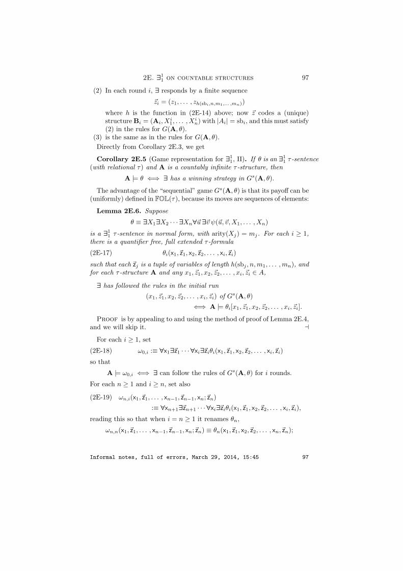
2E. ∃11 on countable structures 97
(2) In each round i, ∃ responds by a finite sequence
~zi = (z1, . . . , zh(sbi,n,m1,... ,mn))
where h is the function in (2E-14) above; now ~z codes a (unique)structure Bi = (Ai, X
i1, . . . , Xi
n) with |Ai| = sbi, and this must satisfy(2) in the rules for G(A, θ).
(3) is the same as in the rules for G(A, θ).Directly from Corollary 2E.3, we get
Corollary 2E.5 (Game representation for ∃11, II). If θ is an ∃1
1 τ -sentence(with relational τ) and A is a countably infinite τ -structure, then
A |= θ ⇐⇒ ∃ has a winning strategy in Gs(A, θ).
The advantage of the “sequential” game Gs(A, θ) is that its payoff can be(uniformly) defined in FOL(τ), because its moves are sequences of elements:
Lemma 2E.6. Suppose
θ ≡ ∃X1∃X2 · · ·∃Xn∀~u ∃~v ψ(~u,~v,X1, . . . , Xn)
is a ∃11 τ -sentence in normal form, with arity(Xj) = mj. For each i ≥ 1,
there is a quantifier free, full extended τ -formula
θi(x1,~z1, x2,~z2, . . . , xi,~zi)(2E-17)
such that each ~zj is a tuple of variables of length h(sbj , n, m1, . . . , mn), andfor each τ -structure A and any x1, ~z1, x2, ~z2, . . . , xi, ~zi ∈ A,
∃ has followed the rules in the initial run
(x1, ~z1, x2, ~z2, . . . , xi, ~zi) of Gs(A, θ)
⇐⇒ A |= θi[x1, ~z1, x2, ~z2, . . . , xi, ~zi].
Proof is by appealing to and using the method of proof of Lemma 2E.4,and we will skip it. a
For each i ≥ 1, set
ω0,i :≡ ∀x1∃~z1 · · ·∀xi∃~ziθi(x1,~z1, x2,~z2, . . . , xi,~zi)(2E-18)
so that
A |= ω0,i ⇐⇒ ∃ can follow the rules of Gs(A, θ) for i rounds.
For each n ≥ 1 and i ≥ n, set also
(2E-19) ωn,i(x1,~z1, . . . , xn−1,~zn−1, xn;~zn)
:≡ ∀xn+1∃~zn+1 · · ·∀xi∃~ziθi(x1,~z1, x2,~z2, . . . , xi,~zi),
reading this so that when i = n ≥ 1 it renames θn,
ωn,n(x1,~z1, . . . , xn−1,~zn−1, xn;~zn) ≡ θn(x1,~z1, x2,~z2, . . . , xn,~zn);
Informal notes, full of errors, March 29, 2014, 15:45 97
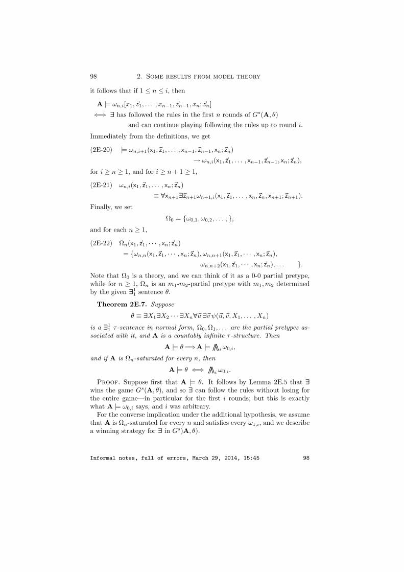
98 2. Some results from model theory
it follows that if 1 ≤ n ≤ i, then
A |= ωn,i[x1, ~z1, . . . , xn−1, ~zn−1, xn;~zn]
⇐⇒ ∃ has followed the rules in the first n rounds of Gs(A, θ)and can continue playing following the rules up to round i.
Immediately from the definitions, we get
(2E-20) |= ωn,i+1(x1,~z1, . . . , xn−1,~zn−1, xn;~zn)
→ ωn,i(x1,~z1, . . . , xn−1,~zn−1, xn;~zn),
for i ≥ n ≥ 1, and for i ≥ n + 1 ≥ 1,
(2E-21) ωn,i(x1,~z1, . . . , xn;~zn)
≡ ∀xn+1∃~zn+1ωn+1,i(x1,~z1, . . . , xn,~zn, xn+1;~zn+1).
Finally, we set
Ω0 = ω0,1, ω0,2, . . . , ,and for each n ≥ 1,
(2E-22) Ωn(x1,~z1, · · · , xn;~zn)
= ωn,n(x1,~z1, · · · , xn;~zn), ωn,n+1(x1,~z1, · · · , xn;~zn),
ωn,n+2(x1,~z1, · · · , xn;~zn), . . . .Note that Ω0 is a theory, and we can think of it as a 0-0 partial pretype,while for n ≥ 1, Ωn is an m1-m2-partial pretype with m1,m2 determinedby the given ∃1
1 sentence θ.
Theorem 2E.7. Suppose
θ ≡ ∃X1∃X2 · · ·∃Xn∀~u ∃~v ψ(~u,~v,X1, . . . , Xn)
is a ∃11 τ -sentence in normal form, Ω0, Ω1, . . . are the partial pretypes as-
sociated with it, and A is a countably infinite τ -structure. Then
A |= θ =⇒A |= ∧∧i ω0,i,
and if A is Ωn-saturated for every n, then
A |= θ ⇐⇒ ∧∧i ω0,i.
Proof. Suppose first that A |= θ. It follows by Lemma 2E.5 that ∃wins the game Gs(A, θ), and so ∃ can follow the rules without losing forthe entire game—in particular for the first i rounds; but this is exactlywhat A |= ω0,i says, and i was arbitrary.
For the converse implication under the additional hypothesis, we assumethat A is Ωn-saturated for every n and satisfies every ω1,i, and we describea winning strategy for ∃ in Gs)A, θ).
Informal notes, full of errors, March 29, 2014, 15:45 98

2E. ∃11 on countable structures 99
Suppose ∀ moves x1 in round 1, and consider the partial type
Ωx11 (~z1) = ω1,1(x1;~z1), ω1,2(x1;~z1), . . .
of the structure A. By (2E-21) and the hypothesis A |= ω0,i, we get that
A |= ∀x1∃~z1ω1,i(x1,~z1);
and when we apply this to the x1 moved by ∀, we get some ~zi1 such that
A |= ω1,i[x1, ~zi1],
which by (2E-20) implies that
for every j ≤ i,A |= ω1,j [x1, ~zi1].
Thus Ωx11 is finitely satisfiable, hence realized by the hypothesis, and we
have a single ~z1 such that
A |= ω1,i[x1, ~z1] (1 ≤ i);(2E-23)
in particular, A |= θ1[x1, ~z1], and so ∃ can move z1 and not lose on the firstround.
We now proceed recursively to show how, for each n, ∃ can respond to∀’s first n moves following the rules, and so that if ∀ moves some xn+1,then the partial type
(2E-24) Ωx1,z1,... ,xn,zn,xn+1n+1 (~zn+1)
= ωn+1,n+1(x1,~z1, · · · , xn,~zn, xn+1;~zn+1),
ωn+1,n+2(x1,~z1, · · · , xn,~zn, xn+1;~zn+1),
ωn,n+2(x1,~z1, · · · , xn,~zn, xn+1;~zn+1) . . . is finitely satisfiable, hence realized; ∃ can then move some ~zn+1 which real-izes it, and go on indefinitely without losing—hence, in the end, winning.a
Recall from Section 1K.4 that a relation P ⊆ Ak is ∃11 in a τ -structure
A, if there is a full extended ∃11 formula θ(~y) such that
P (~y) ⇐⇒ A |= θ[~y] (~y ∈ Ak).(2E-25)
Choose fresh constants ~d ≡ (d1, . . . , dk), and for each ~x ∈ Ak, let (A, ~y) bethe (τ, ~d) structure in which ~d := ~y, so that
P (~y) ⇐⇒ A |= θ[~y] ⇐⇒ (A, ~y) |= θ(~d).(2E-26)
Theorem 2E.8. Suppose A is a countably infinite τ -structure and sup-pose P ⊆ An is a ∃1
1 relation on A, defined by (2E-25); it follows that
P (~x) ⇐⇒ ∃ has a winning strategy in G((A, ~x), θ(~d))
⇐⇒ ∃ has a winning strategy in Gs((A, ~x), θ(~d)).
Informal notes, full of errors, March 29, 2014, 15:45 99

100 2. Some results from model theory
Theorem 2E.7 has a similar interpretation for ∃11 relations on sufficiently
saturated structures:
Theorem 2E.9. Suppose τ is a relational signature and θ(~y) is a fullextended ∃1
1 τ -formula; then there is a sequence
Ωθn(~y, x1,~z1, · · · , xn;~zn) (n ≥ 0)
of partial pretypes, such that if A is a countably infinite structure which isΩθ
n-saturated for every n, then
A |= θ[~y] ⇐⇒ A |= ∧∧Ωθ[~y].
It follows that if A is Ωθn-saturated for every ∃1
1 formula θ(~y) and every n,then every ∃1
1 relation on A is a conjunction of a sequence of A-elementaryrelations.
2F. Craig interpolation and Beth definability (via games)
We use here Theorem 2E.9 to prove the following, basic result:
Theorem 2F.1 (The Craig Interpolation Theorem). Suppose τ is a re-lational signature, T is a τ -theory which has no finite models, and
T ` φ(~Y ) → ψ( ~X),(2F-27)
where the sentences
φ(~Y ) ≡ φ(Y1, . . . , Ym) and ψ( ~X) ≡ ψ(X1, . . . , Xn)
may have symbols from τ in addition to the (fresh, distinct) relation symbolsexhibited. There is then a τ -sentence χ, such that
T ` φ(~Y ) → χ and T ` χ → ψ( ~X).
One of the (many) important consequences of this result is the following:
Theorem 2F.2 (The Beth Definability Theorem). Suppose φ(X) is asentence in FOL(τ ∪ X), where the n-ary relation symbol X is not inthe (relational) signature τ , T is a τ -theory with no finite models, and
T ` φ(X) & φ(Y ) → (∀~x)[X(~x) ↔ Y (~x)];
there is then a full extended τ -formula χ(~x) such that
T ` φ(X) → (∀~x)[X(~x) ↔ χ(~x)].
Somewhat loosely (and skipping the conditions on T , which can be re-moved), if at most one relation X satisfies φ(X) in every model of T , thensome τ -formula χ(~x) defines this X in every model of T in which it exists.
Informal notes, full of errors, March 29, 2014, 15:45 100

2F. Craig interpolation and Beth definability (via games) 101
Proof of 2F.2 from 2F.1. Choose distinct, fresh constants ~d ≡ d1, . . . , dn
and check (easily) that the hypothesis implies
T `(φ(X) & X(~d)
)→
(φ(Y ) → Y (~d)
).
By Theorem 2F.1 then, there is a (τ, ~d)-sentence χ(~d) such that
T `(φ(X) & X(~d)
)→ χ(~d), and T ` χ(~d) →
(φ(Y ) → Y (~d)
),
from which we get (with a bit of logic)
T `(φ(X) & X(~x)
)→ χ(~x), and T `
(χ(~x) & φ(X)
)→ X(~x),
which (with a bit of logic, again) yields the required result. aThe proof of Theorem 2F.1 will be based on the following version of
Theorem 2E.7, for ∀11-sentences:
Theorem 2F.3. Suppose τ is a relational signature and η is a ∀11 τ -
sentence. There exists a sequence Ω0, Ω1, . . . of partial pretypes and a se-quence of τ -sentences η0, η1, . . . , such that
|= ηi → ηi+1 (i = 0, 1, . . . );
for every countably infinite τ -structure A and every i,
A |= ηi → η;
and if A is Ωn-saturated for every n, then
A |= η ⇐⇒ A |= ∨∨i ηi.
Proof. Apply Theorem 2E.7 to the ∃11 τ -sentence θ which is logically
equivalent to ¬η, use the partial pretypes Ωn constructed for the proof ofthat result, and set
ηi ≡ ¬ω0,i.
Now
|= ηi → ηi+1
by (the contrapositive of) (2E-20), with n = 0;
A |= ηi → η
for every countably infinite A by the (contrapositive of) the first part ofTheorem 2E.7; and if A is Ωn-saturated for every n, then
A |= η ⇐⇒ not A |= θ ⇐⇒ not A |= ∧∧i ω0,i
⇐⇒ A |= ∨∨i ¬ω0,i ⇐⇒ A |= ∨∨
i ηi. a
Informal notes, full of errors, March 29, 2014, 15:45 101

102 2. Some results from model theory
Proof of Theorem 2F.1. The hypothesis implies immediately that
T |= ∃~Y φ(~Y ) → ∀ ~Xψ( ~X),
so apply Theorem 2F.3 to η ≡ ∀ ~Xψ( ~X) to get Ω0, Ω1, . . . and η0, η1, . . . ,with the properties enumerated in that result. One of them is that, forevery i and every countable, infinite τ -structure A,
A |= ηi → η;
so to complete the proof, it is enough to show thatClaim: There is some i, such that if A′ is any countably infinite model
of T , then
A′ |= ∃~Y φ(~Y ) → ηi.
Proof of the Claim. If not, then the theory
T = φ(Y ),¬η0,¬η1,¬η2, . . . is consistent (appealing to |= ηi → ηi+1), and so it has a countably infinitemodel (A′, ~Y ′). By the basic Theorem 2C.7 (which is the key to this proof),(A′, ~Y ′) has an elementary extension (A, ~Y ′′) which is Ωn-saturated forevery Ωn associated with η in Theorem 2F.3; in particular, A |= T , and(A, ~Y ′′) |= φ(~Y ), which means that A |= ∃~Y φ(~Y ). The hypothesis of thetheorem now implies that A |= ∀ ~Xψ( ~X), which by the saturation givesA |= ∨∨
i ηi, contradicting our assumption. a
Problems for Section 2F
Problem x2F.1. Prove that the class of ∃11 relations P (~x, ~R) on a τ -
structure A is closed under substitution of A-elementary functions, as wellas the positive operations
& , ∨ , ∃v, ∀v, ∃X;
similarly, the class of ∀11 relations on A is closed under substitution of
A-elementary functions and the operations
& , ∨ , ∃v, ∀v, ∀X.
Hint: You will need some fairly simple logical equivalences, including
(∀u)(∃X)P (u, X) ⇐⇒ (∃Y )(∀u)P (u, ~v | Y (u,~v))(2F-28)
where X ranges over n-ary and Y ranges over (n+1)-ary relations. To usethis in the formal language, you will need to associate with each extendedFOL2-formula φ(X) and each variable u (which does not occur in φ(X)),an extended formula
φ∗(Y ) ≡ φ(~v | Y (u,~v)),
Informal notes, full of errors, March 29, 2014, 15:45 102

2F. Craig interpolation and Beth definability (via games) 103
in which X does not occur, Y is fresh, and for all structures A and allassignments π,
A, πu := x,X := R |= φ ⇐⇒ A, πu := x, Y := (x, ~y) | ~x ∈ X |= φ∗.
(The construction of φ∗ is by structural recursion on φ.)
Informal notes, full of errors, March 29, 2014, 15:45 103


CHAPTER 3
INTRODUCTION TO THE THEORY OF PROOFS
In order to study proofs as mathematical objects, it is necessary to in-troduce deductive systems which are richer and model better the intuitiveproofs we give in mathematics than the Hilbert system of Chapter 1. Our(limited) aim in this chapter is to formulate and establish in outline a cen-tral result of Gentzen, which in addition to its foundational significancealso has a large number of applications.
3A. The Gentzen Systems
The main difference between the Hilbert proof system and the Gentzensystems G and GI is in the proofs, which Gentzen endows with a rich, com-binatorial structure that facilitates their mathematical study. It will alsobe convenient, however, to enlarge the language FOL(τ) with a sequenceof propositional variables
p1, p1, . . . ,
so that the Propositional Calculus is naturally embedded in FOL(τ), for anysignature τ . So the formulas of FOL(τ) are now defined by the recursion
χ :≡ p | s = t | R(t1, . . . , tn) (the prime formulas)
| ¬(φ) | (φ) → (ψ) | (φ) & (ψ) | (φ) ∨ (ψ) | ∀vφ | ∃vφ
where p is any propositional variable; and in the semantics of the system, weadmit assignments which in addition to their values on individual variablesalso assign a truth value π(p) (either t or f) to every propositional variablep.
We should also note that the identity symbol is treated like any otherrelation constant by the Gentzen systems, i.e., we do not postulate theAxioms for Identity and we will need to include them among the hypotheseswhen they are relevant.
105
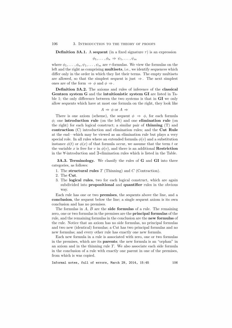
106 3. Introduction to the theory of proofs
Definition 3A.1. A sequent (in a fixed signature τ) is an expression
φ1, . . . , φn ⇒ ψ1, . . . , ψm
where φ1, . . . , φn, ψ1, . . . , ψm are τ -formulas. We view the formulas on theleft and the right as comprising multisets, i.e., we identify sequences whichdiffer only in the order in which they list their terms. The empty multisetsare allowed, so that the simplest sequent is just ⇒ . The next simplestones are of the form ⇒ φ and φ ⇒ .
Definition 3A.2. The axioms and rules of inference of the classicalGentzen system G and the intuitionistic system GI are listed in Ta-ble 1; the only difference between the two systems is that in GI we onlyallow sequents which have at most one formula on the right, they look like
A ⇒ φ or A ⇒There is one axiom (scheme), the sequent φ ⇒ φ, for each formula
φ; one introduction rule (on the left) and one elimination rule (onthe right) for each logical construct; a similar pair of thinning (T) andcontraction (C) introduction and elimination rules; and the Cut Ruleat the end—which may be viewed as an elimination rule but plays a veryspecial role. In all rules where an extended formula φ(v) and a substitutioninstance φ(t) or φ(x) of that formula occur, we assume that the term t orthe variable x is free for v in φ(v), and there is an additional Restrictionin the ∀-introduction and ∃-elimination rules which is listed in the Table.
3A.3. Terminology. We classify the rules of G and GI into threecategories, as follows:
1. The structural rules T (Thinning) and C (Contraction).2. The Cut.3. The logical rules, two for each logical construct, which are again
subdivided into propositional and quantifier rules in the obviousway.
Each rule has one or two premises, the sequents above the line, and aconclusion, the sequent below the line; a single sequent axiom is its ownconclusion and has no premises.
The formulas in A, B are the side formulas of a rule. The remainingzero, one or two formulas in the premises are the principal formulas of therule, and the remaining formulas in the conclusion are the new formulas ofthe rule. Notice that an axiom has no side formulas, no principal formulasand two new (identical) formulas; a Cut has two principal formulas and nonew formulas; and every other rule has exactly one new formula.
Each new formula in a rule is associated with zero, one or two formulasin the premises, which are its parents; the new formula is an “orphan” inan axiom and in the thinning rule T . We also associate each side formulain the conclusion of a rule with exactly one parent in one of the premises,from which is was copied.
Informal notes, full of errors, March 29, 2014, 15:45 106

3A. The Gentzen Systems 107
The Gentzen Systems G, GI
Axiom Scheme φ ⇒ φ
→ A, φ ⇒ B, ψ
A ⇒ B, φ → ψ
A1 ⇒ B1, φ A2, ψ ⇒ B2
A1, A2, φ → ψ ⇒ B1, B2
&A ⇒ B, φ A ⇒ B, ψ
A ⇒ B, φ & ψ
φ, A ⇒ B
φ& ψ, A ⇒ B
ψ, A ⇒ B
φ& ψ, A ⇒ B
∨ A ⇒ B, φ
A ⇒ B, φ ∨ ψ
A ⇒ B, ψ
A ⇒ B, φ ∨ ψ
A, φ ⇒ B A, ψ ⇒ B
A, φ ∨ ψ ⇒ B
¬ A, φ ⇒ B
A, ⇒ B, ¬φ
A ⇒ B, φ
A, ¬φ ⇒ B
∀ A ⇒ B, φ(v)A ⇒ B, ∀xφ(x)
(Restr)A, φ(t) ⇒ B
A, ∀xφ(x) ⇒ B
∃ A ⇒ B, φ(t)A ⇒ B, ∃xφ(x)
A, φ(v) ⇒ B
A, ∃xφ(x) ⇒ B(Restr)
TA ⇒ B
A ⇒ B, φ
A ⇒ B
A, φ ⇒ B
CA ⇒ B, φ, φ
A ⇒ B, φ
A, φ, φ ⇒ B
A, φ ⇒ B
CutA1 ⇒ B1, χ, χ, A2 ⇒ B2
A1, A2 ⇒ B1, B2
(1) A,B are multisets of formulas in FOL(τ).(2) For the Intuitionistic system GI, at most one formula is allowed on
the right.(3) Restr : the active variable v is not free in A,B.(4) The formulas in A,B are the side formulas of an inference.(5) The formulas φ, ψ above the line are the principal formulas of the
inference. (One or two; none in the axiom.)(6) There is an obvious new formula below the line in each inference,
except for Cut.(7) Each new and each side formula in the conclusion of each rule is
associated with zero, one or two parent formulas in the premises.
Table 1. The Gentzen systems.
Informal notes, full of errors, March 29, 2014, 15:45 107

108 3. Introduction to the theory of proofs
Definition 3A.4 (Proofs). The set of Gentzen proofs of depth ≤ dand the endsequent of each proof are defined together by the followingrecursion on the natural number d ≥ 1.
1. For each formula φ, the pair (∅, φ ⇒ φ) is a proof of depth ≤ 1 andendsequent φ ⇒ φ. We picture it in tree form by:
φ ⇒ φ
2. If Π is a proof of depth ≤ d and endsequent α and
αβ
is a one-premise inference rule, then the pair (Π, β) is a proof of depth≤ (d + 1) and endsequent β. We picture (Π, β) in tree form by:
Πβ
.
3. If Π1, Π2 are proofs of depth ≤ d and respective endsequents α1, α2,and if
α1 α2
β
is a two-premise inference rule, then the pair ((Π1, Π2), β) is a proofof depth ≤ (d + 1). We picture ((Π1, Π2), β) in tree form by:
Π1 Π2
β
A proof Π in G of GI is a proof of depth d, for some d, and it is a proofof its endsequent; it is a propositional proof if none of the four rulesabout the quantifiers are used in it. We denote the relevant relations by
G ` A ⇒ B, G `prop A ⇒ B, GI ` A ⇒ B, or GI `prop A ⇒ B
accordingly.We let Gprop and GIprop be the restricted systems in which only for-
mulas for the Propositional Calculus 1K.2 and only propositional rules areallowed.
Proposition 3A.5 (Parsing for Gentzen proofs). Each proof Π satis-fies exactly one of the following three conditions.
1. Π = (∅, β), where β is an axiom.2. Π = (Σ, β), where Σ is a proof of smaller depth and endsequent some
α, and there is a one premise ruleαβ
.
Informal notes, full of errors, March 29, 2014, 15:45 108

3A. The Gentzen Systems 109
3. Π = ((Σ1, Σ2), β), where Σ1, Σ2 are proofs of smaller depth and re-
spective endsequents α1, α2, and there is a two premise ruleα1 α2
β.
In all cases, a proof is a pair and the second member of that pair is itsendsequent.
Proofs in the Gentzen systems are displayed in tree form, as in the fol-lowing examples which prove in G three of the propositional axioms of theHilbert system:
χ ⇒ χ(⇒ ¬)⇒ χ,¬χ(¬ ⇒)¬¬χ ⇒ χ
(⇒→)⇒ ¬¬χ → χ
φ ⇒ φ(T )
φ, ψ ⇒ φ(⇒→)
φ ⇒ ψ → φ(⇒→)
⇒ φ → (ψ → φ)
φ ⇒ φ(T )
φ, ψ ⇒ φ
ψ ⇒ ψ(T )
φ, ψ ⇒ ψ(⇒ &)
φ, ψ ⇒ φ & ψ(⇒→)
φ ⇒ ψ → (φ & ψ)(⇒→)
⇒ φ → (ψ → (φ & ψ))
Notice that the first of these proofs is in G, while the last two are in GI.In the next example of a GI-proof of another of the Hilbert propositional
axioms we do not label the rules, but we put in boxes the principal formulasfor each application:
φ ⇒ φ
φ ⇒ φ
ψ ⇒ ψ χ ⇒ χ
ψ, ψ → χ ⇒ χ
φ, ψ , φ → (ψ → χ) ⇒ χ
φ , φ → ψ, φ → (ψ → χ) ⇒ χ
φ → ψ, φ → (ψ → χ) ⇒ φ → χ
φ → ψ ⇒ φ → (ψ → χ) → (φ → χ)
⇒ (φ → ψ) → ((φ → (ψ → χ)) → (φ → χ))
The form of the rules of inference in the Gentzen systems makes it mucheasier to discover proofs in them rather than in the Hilbert system. Con-sider, for example, the following, which can be constructed step-by-step
Informal notes, full of errors, March 29, 2014, 15:45 109

110 3. Introduction to the theory of proofs
starting with the last sequent (which is what we want to show) and tryingout the most plausible inference which gives it:
φ ⇒ φ(∀ ⇒)
∀vφ ⇒ φ ⇒ ∃)∀vφ ⇒ ∃uφ
(∃ ⇒, u not free on the right)∃u∀vφ ⇒ ∃uφ
(⇒ ∀, v not free on the left)∃u∀vφ ⇒ ∀v∃uφ
(⇒→)⇒ ∃u∀vφ → ∀v∃uφ
In fact these guesses are unique in this example, except for Thinnings,Contractions and Cuts, and it is quite common that the most difficultproofs to construct are those which required T’s and C’s—especially as wewill show that Cuts are not necessary.
Theorem 3A.6 (Strong semantic soundness of G). Suppose
G ` φ1, . . . , φn ⇒ ψ1, . . . , ψm,
and A is any structure (of the fixed signature): then for every assignmentπ into A,
if A, π |= φ & . . . & φn, then A, π |= ψ ∨ . . . ∨ ψm.
Here the empty conjunction is interpreted by t and the empty disjunctionis interpreted by f.
Theorem 3A.7 (Proof-theoretic soundness of G). If G ` A ⇒ B,then A ` ∨B in the Hilbert system, by a deduction in which no free variableof A is quantified and the Identity Axioms (5) – (17) are not used.
Theorem 3A.8 (Proof-theoretic completeness of G). If A ` φ in theHilbert system by a deduction in which no free variable of A is quantifiedand the Identity Axioms (5) – (17) are not used, then G ` A ⇒ φ.
These three theorems are all proved by direct (and simple, if a bit cum-bersome) inductions on the given proofs.
3A.9. Remark. The condition in Theorem 3A.8 is necessary, because(for example)
R(x) ` ∀xR(x)(3A-1)
but the sequentR(x) ⇒ ∀xR(x)
is not provable in G, because of the strong Soundness Theorem 3A.6. TheHilbert system satisfies the following weaker Soundness Theorem, whichdoes not contradict the deduction (3A-1): if A ` φ and every assignmentπ into A satisfies A, then every assignment π into A satisfies φ. (We have
Informal notes, full of errors, March 29, 2014, 15:45 110

3B. Cut-free proofs 111
stated the Soundness Theorem for the Hilbert system in 4.3 only for setsof sentences as hypotheses, but to prove it we needed to show this strongerstatement.)
Theorem 3A.10 (Semantic Completeness of G). Suppose ψ, φ1, . . . , φn
are τ -formulas such that for every τ -structure A and every assignment πinto A,
if A, π |= φ1 & · · · & φn, then A, π |= ψ;it follows that
G ` IA, φ1, . . . , φn ⇒ ψ,
where IA are the (finitely many) identity axioms for the relation and func-tion symbols which occur in ψ, φ1, . . . , φn.
Proof This follows easily from Theorem 3A.8 and the CompletenessTheorem for the Hilbert system. a
3A.11. The intuitionistic Gentzen system GI. The system GI isa formalization of L. E. J. Brouwer’s intuitionistic logic, the logical founda-tion of constructive mathematics. This was developed near the beginningof the 20th century. It was Gentzen’s ingenious idea that constructive logiccan be captured simply by restricting the number of formulas on the rightof a sequent. About constructive mathematics, we will say a little morelater on; for now, we just use GI as a tool to understand the combinatorialmethods of analyzing formal proofs that pervade proof theory.
3B. Cut-free proofs
Cut is the only G-rule which “loses the justification” for the truth of itsconclusion, just as Modus Ponens (which is a simple version of it) does inthe Hilbert system. As a result, Cut-free Gentzen proofs (which do not usethe Cut) have important special properties.
Proposition 3B.1. If one of the logical symbols ¬, &, ∨, →, ∀ or ∃does not occur in the endsequent of a Cut-free proof Π, then that logicalsymbol does not occur at all in Π, and hence neither of the rules involvingthat logical symbol are applied in Π.
Definition 3B.2. The subformulas of a formula of FOL(τ) are definedby the following recursion.
1. If χ ≡ p, χ ≡ R(t1, . . . , tn) or χ ≡ s = t is prime, then χ is the onlysubformula of itself.
2. If χ is a propositional combination of φ and ψ, then the subformulasof χ are χ itself, and all the subformulas of φ and ψ.
Informal notes, full of errors, March 29, 2014, 15:45 111

112 3. Introduction to the theory of proofs
3. If χ ≡ ∃xφ(x) or χ ≡ ∀xφ(x), then the subformulas of χ are χ andall subformulas of substitution instances φ(t), where t is an arbitraryterm, free for x in φ(x). (Here t may be a variable, since variables areterms, and in particular φ(x) is a subformula of χ.)
For example, the subformulas of ∃xR(x, y) are all R(t, y), and there areinfinitely many of them; if a formula has only finitely many subformulas,then it is propositional.
Theorem 3B.3 (Subformula Property). If Π is a Cut-free proof withendsequent α, then every formula which occurs in Π is a subformula of someformula in α.
Corollary 3B.4. If a constant c, a relation symbol R or a functionsymbol f does not occur in the endsequent of a Cut-free proof Π, then c, Ror f does not occur at all in Π.
3C. Cut Elimination
We outline here (with few details) a proof of the following, fundamentaltheorem of Gentzen, to the effect that up to alphabetic changes in boundvariables, every provable sequent has a Cut-free proof:
Theorem 3C.1 (Cut Elimination Theorem, Gentzen’s Hauptsatz).From a proof in G or GI of a sequent α in which no variable occurs bothfree and bound, we can construct a pure variable, Cut-free proof of α in thesame system.
Pure variable proofs will be defined below in Definition 3C.8.This is the basic result of Proof Theory, and it has a host of important
consequences in all parts of logic (and some parts of classical mathematicsas well).
3C.2. The Mix rule. This is a strengthening of the Cut rule, whichallows us to Cut simultaneously all occurrences of the Cut formula:
A1 ⇒ B1 A2 ⇒ B2
A1, A2 \ χ ⇒ B1 \ χ, B2assuming that χ ∈ A2 ∩B1.
For a multiset D, by D\χ we mean the result of removing all occurrencesof χ from D.
By Gm and GIm we understand the systems in which the Cut Rule hasbeen replaced by the Mix Rule.
Lemma 3C.3. If we replace the Cut Rule by the Mix Rule, we get ex-actly the same provable sequents, both for G and for GI.
Informal notes, full of errors, March 29, 2014, 15:45 112
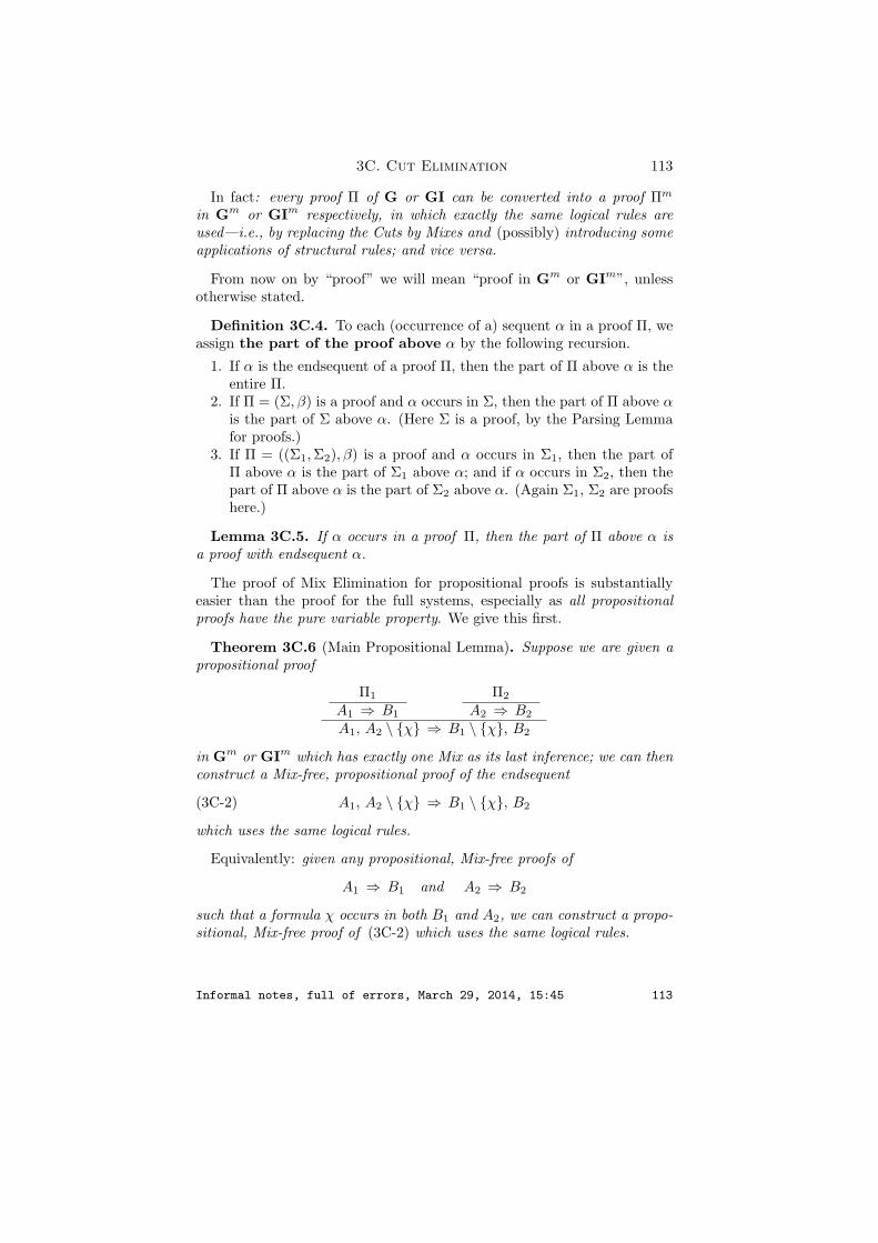
3C. Cut Elimination 113
In fact: every proof Π of G or GI can be converted into a proof Πm
in Gm or GIm respectively, in which exactly the same logical rules areused—i.e., by replacing the Cuts by Mixes and (possibly) introducing someapplications of structural rules; and vice versa.
From now on by “proof” we will mean “proof in Gm or GIm”, unlessotherwise stated.
Definition 3C.4. To each (occurrence of a) sequent α in a proof Π, weassign the part of the proof above α by the following recursion.
1. If α is the endsequent of a proof Π, then the part of Π above α is theentire Π.
2. If Π = (Σ, β) is a proof and α occurs in Σ, then the part of Π above αis the part of Σ above α. (Here Σ is a proof, by the Parsing Lemmafor proofs.)
3. If Π = ((Σ1, Σ2), β) is a proof and α occurs in Σ1, then the part ofΠ above α is the part of Σ1 above α; and if α occurs in Σ2, then thepart of Π above α is the part of Σ2 above α. (Again Σ1, Σ2 are proofshere.)
Lemma 3C.5. If α occurs in a proof Π, then the part of Π above α isa proof with endsequent α.
The proof of Mix Elimination for propositional proofs is substantiallyeasier than the proof for the full systems, especially as all propositionalproofs have the pure variable property. We give this first.
Theorem 3C.6 (Main Propositional Lemma). Suppose we are given apropositional proof
Π1
A1 ⇒ B1
Π2
A2 ⇒ B2
A1, A2 \ χ ⇒ B1 \ χ, B2
in Gm or GIm which has exactly one Mix as its last inference; we can thenconstruct a Mix-free, propositional proof of the endsequent
A1, A2 \ χ ⇒ B1 \ χ, B2(3C-2)
which uses the same logical rules.
Equivalently: given any propositional, Mix-free proofs of
A1 ⇒ B1 and A2 ⇒ B2
such that a formula χ occurs in both B1 and A2, we can construct a propo-sitional, Mix-free proof of (3C-2) which uses the same logical rules.
Informal notes, full of errors, March 29, 2014, 15:45 113

114 3. Introduction to the theory of proofs
Outline of the proof. We define the left Mix rank to be the numberof consecutive sequents in the proof which ends with A1 ⇒ B1 startingfrom the last one and going up, in which χ occurs on the right; so this isat least 1. The right Mix rank is defined similarly, and the rank of the Mixis their sum. The minimum Mix rank is 2. The grade of the Mix is thenumber of logical symbols in the Mix formula χ.
The proof is by induction on the grade. Both in the basis (when χ is aprime formula) and in the induction step, we will need an induction on therank, so that the proof really is by double induction.
Lemma 1. If the Mix formula χ occurs in A1 or in B2, then we caneliminate the Mix using Thinnings and Contractions.
Lemma 2. If the left Mix rank is 1 and the last left inference is by a Tor a C, then the Mix can be eliminated; similarly if the right Mix rank is 1and the last right inference is a C or a T. (Actually the last left inferencecannot be a C if the left Mix rank is 1.)
Main part of the proof. We now consider cases on what the last leftinference and the last right inference is, and we may assume that the MainLemma holds for all cases of smaller grade, and for all cases of the samegrade but smaller rank. The cases where one of the ranks is > 1 are treatedfirst, and are messy but fairly easy. The main part of the proof is in theconsideration of the four cases (one for each propositional connective) wherethe rank is exactly 2, so that χ is introduced by the last inference on bothsides: in these cases we use the induction hypothesis on the grade, reducingthe problem to cases of smaller grade (but possibly larger rank). a
Proof of Theorem 3C.1 for propositional proofs is by induc-tion on the number of Mixes in the given proof, with the basis given byLemma 3C.6; in the Inductive Step, we simply apply the same Lemma toan uppermost Mix, one such the part of the proof above its conclusion hasno more Mixes. a
The proof of the Hauptsatz for the full (classical and intuitionistic) sys-tems is complicated by the extra hypothesis on free-and-bound occurrencesof the same variable, which is necessary because of the following examplewhose proof we will leave for the problems:
Proposition 3C.7. The sequent ∀x∀yR(x, y) ⇒ R(y, y) is provable inGI, but it is not provable without a Cut (even in the stronger system G).
To deal with this problem, we need to introduce a “global” restrictionon proofs, as follows.
3C.8. Definition. A pure variable proof (in any of the four Gentzensystems we have introduced) is a proof Π with the following two properties.
Informal notes, full of errors, March 29, 2014, 15:45 114

3C. Cut Elimination 115
1. No variable occurs both free and bound in Π.2. If v is the active variable in an application of one of the two rules
which have a restriction,
A ⇒ B, φ(v)A ⇒ B, ∀xφ(x)
orA, φ(v) ⇒ B
A, ∃xφ(x) ⇒ B,
then v occurs only in the part of the proof above the premise of thisapplication.
Lemma 3C.9. In a pure variable proof, a variable v can be used at mostonce in an application of the ⇒ ∀ or the ∃ ⇒ rules.
Proposition 3C.10 (Pure Variable Lemma). If α is a sequent in whichno variable occurs both free and bound, then from every proof of α we canconstruct a pure variable proof of α, employing only replacement of somevariables by fresh variables.
With this result at hand, we can establish an appropriate version ofLemma 3C.6 which applies to the full systems:
Theorem 3C.11 (Main Lemma). Suppose we are given a pure variableproof
Π1
A1 ⇒ B1
Π2
A2 ⇒ B2
A1, A2 \ χ ⇒ B1 \ χ, B2
in Gm or GIm which has exactly one Mix as its last inference; we can thenconstruct a Mix-free, pure variable proof of the endsequent
A1, A2 \ χ ⇒ B1 \ χ, B2(3C-3)
which uses the same logical rules.
Equivalently: from any given, pure variable, Mix-free proofs of
A1 ⇒ B1 and A2 ⇒ B2
such that a formula χ occurs in both B1 and A2 and no free variable ofone of them occurs bound in the other, we can construct a pure variable,Mix-free proof of (3C-3) which uses the same logical rules.
The proof of this is an extension of the proof of Lemma 3C.6 whichrequires the consideration of two, additional cases in the induction stepwith rank 2—quite simple, as it happens, because the quantifier rules haveonly one premise.
Outline of proof of Theorem 3C.1. It is enough to prove the the-orem for pure variable proofs in the system with Mix instead of Cut; andwe do this by induction on the number of Mixes in the given, pure variableproof, using the Main Lemma 3C.11. a
Informal notes, full of errors, March 29, 2014, 15:45 115

116 3. Introduction to the theory of proofs
3D. The Extended Hauptsatz
For sequents of formulas in prenex form, the Gentzen Hauptsatz providesa particularly simple and useful form.
3D.1. Normal proofs. A proof Π in G is normal if it is a purevariable, Cut-free proof and a midsequent A∗ ⇒ B∗ occurs in it with thefollowing properties.
1. Every formula which occurs above the midsequent A∗ ⇒ B∗ is quan-tifier free.
2. The only rules applied below the midsequent are quantifier rules orContractions.
Notice that by the first of these properties, no quantifier rules are appliedin a normal proof above the midsequent—only propositional and structuralrule applications. So a normal proof looks like
ΠA∗ ⇒ B∗
...A ⇒ B
where Π is a propositional proof and in the “linear trunk” which followsthe provable, quantifier-free sequent only one-premise Contractions andquantifier inferences occur.
Theorem 3D.2 (The Extended Hauptsatz). If A ⇒ B is a sequent ofprenex formulas in which no variable occurs both free and bound, and ifA ⇒ B is provable in G, then there exists a normal proof of A ⇒ B.
Outline of proof. This is a constructive argument, which producesthe desired normal proof of A ⇒ B from any given proof of it.
Step 1. By the Cut Elimination Theorem we get a new proof, which isCut-free and pure variable.
Step 2. We replace all Axioms and all Thinnings by Axioms and Thin-nings on prime (and hence quantifier free) formulas (without destroyingthe Cut-free, pure variable property).
The order of a quantifier rule application in the proof is the number ofThinnings and propositional inferences below it, down to the endsequent,and the order of the proof is the sum of the orders of all quantifier ruleapplications in the proof. If the order of the proof is 0, then there isno quantifier rule application above a Thinning or a propositional ruleapplication, and then the proof (easily) is normal.
Proof is by induction on the order of the given proof. We begin by notic-ing that if the order is > 0, then there must exist some quantifier rule
Informal notes, full of errors, March 29, 2014, 15:45 116

3D. The Extended Hauptsatz 117
application immediately above a Thinning or a propositional rule applica-tion; we choose one such, and alter the proof to one with a smaller orderand the same endsequent. The heart of the proof is the consideration ofcases on what these two inferences immediately above each other are, thetop one a quantifier rule application and the bottom one a propositionalrule application or a T . It is crucial to use the fact that all the formulasin the endsequent are prenex, and hence (by the subformula property) allthe formulas which occur in the proof are prenex; this eliminates a greatnumber of inference pairs. a
This proof of the Extended Hauptsatz uses the permutability of inferencesproperty of the Gentzen systems, which has many other applications.
Theorem 3D.3 (Herbrand’s Theorem). If a prenex formula
θ ≡ (Q1x1) · · · (Qnxn)φ(x1, . . . , xn)
is provable in FOL without the Axioms of Identity (15) – (17) , then thereexists a quantifier free tautology of the form
φ∗ ≡ φ1 ∨ · · · ∨ φn
such that:
(1) Each φi is a substitution instance of the matrix φ(x1, . . . , xn) of θ,and
(2) θ can be proved from φ∗ by the use of the following four Herbrandrules of inferences which apply to disjunctions of formulas:
ψ1(t) ∨ · · · ∨ ψn
∃xψ(x) ∨ · · ·χ · · · ∨ ψn(∃)
ψ1 ∨ · · ·χ1 ∨ χ2 · · · ∨ ψn
ψ ∨ · · ·χ2 ∨ χ1 · · · ∨ ψn(I)
ψ1 ∨ · · ·χ ∨ χ ∨ ψn
ψ1 ∨ · · ·χ · · · ∨ ψn(C)
ψ1(v) ∨ · · · ∨ ψn
∀xψ(x) ∨ · · · ∨ ψn(∀) (Restr)
(Restr): The variable v does not occur free in the conclusion.
3D.4. Remarks. The Herbrand rules obviously correspond to theGentzen quantifier rules and Contraction, together with the Interchangerule which we do not need for multiset sequents; and the restriction on the∀-rule is the same, the variable v must not be free in the conclusion. Aprovable disjunction which satisfies the conclusion of the theorem is calleda Herbrand expansion of θ; by extension, we often refer to the midsequentof a Gentzen normal proof as a Herbrand expansion of the endsequent.
There is an obvious version of the theorem for implications of the form
θ1 → θ2
with both θ1, θ2 prenex.
Informal notes, full of errors, March 29, 2014, 15:45 117
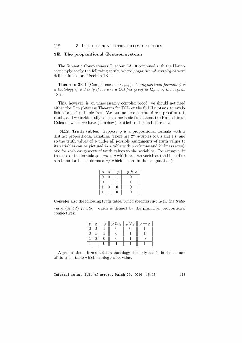
118 3. Introduction to the theory of proofs
3E. The propositional Gentzen systems
The Semantic Completeness Theorem 3A.10 combined with the Haupt-satz imply easily the following result, where propositional tautologies weredefined in the brief Section 1K.2.
Theorem 3E.1 (Completeness of Gprop). A propositional formula φ isa tautology if and only if there is a Cut-free proof in Gprop of the sequent⇒ φ.
This, however, is an unnecessarily complex proof: we should not needeither the Completeness Theorem for FOL or the full Hauptsatz to estab-lish a basically simple fact. We outline here a more direct proof of thisresult, and we incidentally collect some basic facts about the PropositionalCalculus which we have (somehow) avoided to discuss before now.
3E.2. Truth tables. Suppose φ is a propositional formula with ndistinct propositional variables. There are 2n n-tuples of 0’s and 1’s, andso the truth values of φ under all possible assignments of truth values toits variables can be pictured in a table with n columns and 2n lines (rows),one for each assignment of truth values to the variables. For example, inthe case of the formula φ ≡ ¬p & q which has two variables (and includinga column for the subformula ¬p which is used in the computation):
p q ¬p ¬p & q0 0 1 00 1 1 11 0 0 01 1 0 0
Consider also the following truth table, which specifies succinctly the truth-
value (or bit) function which is defined by the primitive, propositionalconnectives:
p q ¬p p & q p ∨ q p → q0 0 1 0 0 10 1 1 0 1 11 0 0 0 1 01 1 0 1 1 1
A propositional formula φ is a tautology if it only has 1s in the columnof its truth table which catalogues its value.
Informal notes, full of errors, March 29, 2014, 15:45 118

3E. The propositional Gentzen systems 119
Outline of Kalmar’s proof of Theorem 3E.1. Fix a list of dis-tinct propositional variables p1, . . . , pn, and for each assignment π, let
πpi ≡
pi, if π(pi) = 1,
¬pi, if π(pi) = 0.
Set
Lineπ(~p) = Lineπ ≡ πp1, πp1, . . . , πpn.(3E-4)
As a multiset, Lineπ expresses formally the hypotheses on the propositionalvariables in the line corresponding to π in the truth table of any formulain which only the letters p1, . . . , pn occur.
Step 1. If only the letters p1, . . . , pn occur in φ, then for every π,
if value(φ, π) = 1, then Gprop ` Lineπ ⇒ φ,
if value(φ, π) = 0, then Gprop ` Lineπ ⇒ ¬φ.
This is proved by an induction on φ which is routine, but necessarilymessy, since it must use every inference rule of Gprop.
For each assignment π to p1, . . . , pn and each i ≤ n, let
Li(π) = πpi+1, πpi+2, . . . , πpn,
so that
L0(π) ≡ Line(π), Ln(π) = ∅,and for every i < n,Li(π) ≡ πpi, Li+1(π).
Step 2. If only the letters p1, . . . , pn occur in φ and φ is a propositionaltautology, then for every i ≤ n and for every assignment π,
Li(π) ⇒ φ
is provable in Gprop.
This is proved by induction on i ≤ n, simultaneously for all assignments,and the Basis Case is Step 1, while the last Case i = n gives the requiredresult. For the inductive step, the Induction Hypothesis applied to the twoassignments
πpi := 1, πpi := 0gives us proofs of
pi, Li+1(π) ⇒ φ and ¬pi, Li+1(π) ⇒ φ,
since φ is a tautology; and from these two proofs we easily get a proofof Li+1(π) ⇒ φ in Gprop, which uses a Cut. The proof is completed byappealing to the propositional case of the Hauptsatz 3C.1. a
Informal notes, full of errors, March 29, 2014, 15:45 119

120 3. Introduction to the theory of proofs
Proposition 3E.3. For every valid, quantifier-free τ -formula φ with n,distinct prime subformulas φ1, . . . , φn and no occurrence of the identitysymbol =, there is a propositional tautology ψ with n distinct propositionalvariables such that
φ ≡ ψp1 :≡ φ1, . . . , pn :≡ φn.
3F. Craig Interpolation and Beth definability (via proofs)
The midsequent of a normal proof in G is a valid, quantifier-free formula,and so (by Proposition 3E.3), it can be obtained from a propositional tau-tology by replacing the propositional variables by prime formulas. Thisfact can be used to derive several interesting results about FOL from theirpropositional versions, which are generally much easier to establish. Weillustrate the process here with two, basic results about first order defin-ability.
Theorem 3F.1 (The Propositional Interpolation Theorem). Suppose
φ(~p, ~q) → ψ(~p, ~r)
is a propositional tautology, where we have indicated all the (distinct) letterswhich may occur in the formulas, and there is at least one pi; then thereexists a formula χ(~p) in which none of the q’s or r’s occur, such that
φ(~p, ~q) → χ(~p), χ(~p) → ψ(~p, ~r)
are both tautologies.
For an example: if the given tautology is
p & q → p ∨ r,
we can take χ ≡ p, with which both p & q → p and p → p∨r are tautologies.In fact this is the interpolant which will come out of the general proof inthis case.
Outline of proof. If no assignment π satisfies φ, we can then take
χ(~p) ≡ pi & ¬pi
with the assumed pi which occurs in both φ and ψ. So we may assumethat at least one assignment satisfies φ.
Generalizing the definition of lines in (3E-4) and making explicit theimplied conjunction, we set for each assignment π,
L(π, ~p) ≡ ∧∧Lineπ(~p) ≡ πp1 & πp2 & · · · & πpn.
Notice that, immediately from the definition,
value(L(π, ~p), π) = 1.
Informal notes, full of errors, March 29, 2014, 15:45 120

3F. Craig Interpolation and Beth definability (via proofs)121
We now take χ(~p) to be the disjunction of these conjunctions over all as-signments π which satisfy φ:
χ(~p) ≡ ∨∨L(π, ~p) | value(φ, π) = 1.Clearly, φ → χ(~p) is a tautology, because if value(π, φ) = 1, then L(π, ~p) isone of the disjuncts of χ(~p) and π satisfies it. For the second claim, supposetowards a contradiction that there is a π such that
value(χ(~p), π) = 1, and value(ψ, π) = 0;
now the definition of χ(~p) implies that value(φ, π) = 1, and so value(ψ, π) =1 by the hypothesis, which is a contradiction. a
Theorem 3F.2 (The Craig Interpolation Theorem). Suppose
|= φ( ~Q, ~f,~c) → ψ(~R,~g, ~d)(3F-5)
where the formulas φ( ~Q, ~f,~c) and ψ(~R,~g, ~d) may have symbols from somesignature τ in addition to the (fresh, distinct) symbols exhibited. There isthen a τ -formula χ such that
|= φ( ~Q, ~f,~c) → χ and |= χ → ψ(~R,~g, ~d).(3F-6)
In fact, from a proof of the implication in (3F-5) in the Hilbert system,we can effectively construct an interpolant χ and proofs of the implicationsin (3F-6).
This is a somewhat stronger version of Theorem 2F.1 in Section 2F, wherewe gave a model-theoretic proof of it using games. It is an important resultand many proofs of it have been published, including one which uses theso-called Robinson Joint Consistency Theorem that we have not includedin these notes. The proof we outline here is Craig’s original argument, andit is distinguished by the fact that it is constructive.
Outline of the proof. We may assume that the formulas in (3F-5)are in prenex form and no variable occurs both free and bound in them.
We will also assume at first that
the equality symbol “=” does not occur in (3F-5),(3F-7)
and then reduce (easily) the general case to this one at the end.The Completeness Theorem, the reduction of the Hilbert system to the
Gentzen system and the Extended Hauptsatz give us from the hypothesisa normal proof
Π : (propositional part) A0 ⇒ B0, A1 ⇒ B1, · · · , An ⇒ Bn,(3F-8)
whose endsequent is (the sequent version of) (3F-5), i.e., An = φ( ~Q, ~f,~c)and Bn = ψ(~R,~g, ~d). The midsequent
A0 ⇒ B0
Informal notes, full of errors, March 29, 2014, 15:45 121

122 3. Introduction to the theory of proofs
of Π is a valid, quantifier-free sequent with no occurrence of =, and so (byProposition 3E.3), there is a valid propositional sequent A∗0 ⇒ B∗
0 fromwhich A0 ⇒ B0 can be obtained by replacing its propositional variableswith prime formulas. Moreover, prime formulas which involve symbols in~Q, ~f,~c occur only in A0, and prime formulas which involve symbols in~R,~g, ~d occur only in B0, and so by the corresponding property for A∗0, B
∗0
and the Propositional Interpolation Theorem 3F.1, there is a propositionalformula χ∗0 whose variables occur both in A∗0 and in B∗
0 such that
G ` A∗0 ⇒ χ∗0; G ` χ∗0 ⇒ B∗0 .
If we now replace again the propositional variables by prime τ -formulas,we get a quantifier-free τ -formula χ0 in which = does not occur and propo-sitional proofs
ΠL0 : · · · , A0 ⇒ χ0, ΠR
0 : · · · , χ0 ⇒ B0(3F-9)
with the indicated endsequents. It is also clear from the construction thatfor every variable v,
if v occurs in χ0, then v occurs free in both A0 and B0.(3F-10)
In the next lemma, Ai, Bi are from the fixed proof (3F-8), and n is thelength of that proof below the midsequent.
Lemma. For each i ≤ n, there is a prenex formula χi and proofs
ΠLi : · · · , Ai ⇒ χi, ΠR
i : · · · , χi ⇒ Bi
with the indicated endsequents so that the following conditions hold:(1) Every relation symbol, function symbol and constant not in the vo-
cabulary τ which occurs in χi occurs in both Ai and Bi.(2) Every free variable of χi occurs free in both Ai and Bi.Proof. We let
Πi = · · · , Ai ⇒ Bi
be the part of the proof Π in (3F-5) up to the stage i. The lemma is provedby (finite) induction on i ≤ n, with the basis given by (3F-9), (3F-10). Inthe Induction Step, we take cases on the inference rule use at step i of Π.
Case 1, Ai+1 ⇒ Bi+1 follows from Ai ⇒ Bi in Π by Contraction onthe right, i.e.,
Πi+1 : · · · , Ai ⇒ B′i, φ, φ, Ai ⇒ B′
i, φ.
In this case we set χi+1 ≡ χi, ΠLi+1 = ΠL
i and construct ΠRi+1 by adding to
ΠRi the Contraction to the right,
ΠRi+1 : · · · , χi ⇒ B′
i, φ, φ, χi ⇒ B′i, φ.
Informal notes, full of errors, March 29, 2014, 15:45 122

3F. Craig Interpolation and Beth definability (via proofs)123
Case 2, Ai+1 ⇒ Bi+1 follows from Ai ⇒ Bi by ⇒∀, i.e.,
Πi+1 : · · · , Ai ⇒ B′i, φ(v), Ai ⇒ B′
i, (∀x)φ(x).
Again, we set χi+1 ≡ χi, ΠLi+1 = ΠL
i , and simply add the new inference toΠR
i ,
ΠRi+1 : · · · , χi ⇒ B′
i, φ(v), Ai ⇒ B′i, (∀x)φ(x).
The Restriction for the rule ⇒∀ insures that v does not occur in Ai andB′
i, and so it also does not occur in χi and this application of the rule inΠR
i+1 is justified.These cases were both trivial, they set χi+1 ≡ χi, and the verification of
Condition (2) in the Lemma at stage i + 1 is immediate—which is why wedid not even mention it.
Case 3, Ai+1 ⇒ Bi+1 follows from Ai ⇒ Bi by ⇒∃, i.e.,
Πi+1 : · · · , Ai ⇒ B′i, φ(t), Ai ⇒ B′
i, (∃x)φ(x).
We first add this inference to ΠRi ,
Σ1 : · · · , χi ⇒ B′i, φ(t), χi ⇒ B′
i, (∃x)φ(x).
This is possible because there are no restrictions on the ⇒∃ rule. Everyfree variable of χi occurs free in Ai, by the induction hypothesis; if everyfree variable of χi also occurs free in B′
i, then we can set
ΠLi+1 = ΠL
i , ΠRi+1 = Σ1,
and the condition (2) in the Lemma is also satisfied at stage i + 1. Butthere may be free variables in the term t which occur in χi and do notoccur in B′
i, and these variables will not occur free in Bi+1 at this stage.So to satisfy Condition (2) at stage i + 1 we need to do something more inthis case.
Suppose v occur free in χi and not in B′i, and so not in B′
i, (∃x)φ(x)either, since v must occur in the term t and so it has been “quantifiedaway”. We can then add to Σ1 an application of ∃⇒ , since the restrictionfor it is satisfied, to get
Σ2 : · · · , χi ⇒ B′i, φ(t), χi ⇒ B′
i, (∃x)φ(x), (∃v)χ ⇒ B′i, (∃x)φ(x).
We do this successively for all the variables which occur free in χ and notin B′
i, to get finally a proof
ΠRi+1 : · · · , (∃v1)(∃v2) · · · (∃vk)χi ⇒ B′
i, (∃x)φ
and set χi+1 ≡ (∃v1)(∃v2) · · · (∃vk)χi. We then extend ΠLi by the corre-
sponding applications of the ⇒∃ rule (which has no restrictions) to get
ΠLi+1 : · · · , Ai ⇒ χi, · · ·Ai ⇒ (∃v1)(∃v2) · · · (∃vk)χi.
Informal notes, full of errors, March 29, 2014, 15:45 123

124 3. Introduction to the theory of proofs
There are three symmetric cases “on the left”, ie when the rule at stagei+1 of Π is a Contraction on the left, an ∃⇒ or a ∀⇒ . They are handledsymmetrically, and they add universal quantifiers to the interpolant χ.
a (Lemma)
The lemma yields immediately the theorem when = does not occur inthe given formulas. If it does, we argue as follows.
By Theorem 3A.10 (the Semantic Completeness of G),
G ` IA(τ), IA( ~Q, ~f,~c), IA(~R,~g, ~d) ⇒(φ( ~Q, ~f,~c) → ψ(~R,~g, ~d)
),
where IA(τ) are the equality axioms for the symbols of τ that occur in φ
and ψ, IA( ~Q, ~f,~c) are the equality axioms for the indicated fresh symbols,etc. It is quite simple to see from this that
G ` IA(τ) & IA( ~Q, ~f,~c) & φ ⇒(IA(~R,~g, ~d) → ψ
).
The proof in G of this sequent treats = as if it were an arbitrary binaryrelation symbol, and so the theorem for the restricted case applies: and ityields a τ -formula χ (perhaps with =) such that
G ` IA(τ) & IA( ~Q, ~f,~c) & φ ⇒ χ, G ` χ ⇒(IA(~R,~g, ~d) → ψ
)
as required. aTheorem 3F.3 (The Beth Definability Theorem). Suppose φ(R) is a sen-
tence in FOL(τ ∪ R), where the n-ary relation symbol R is not in thesignature τ , and the sentence
φ(R) & φ(S) → (∀~x)[R(~x) ↔ S(~x)](3F-11)
is provable (or equivalently valid). From any proof of it we can construct aformula χ(~x) in FOL(τ) such that
φ(R) → (∀~x)[R(~x) ↔ χ(~x)](3F-12)
is provable.
This is the same as Theorem 2F.2 in Section 2F and we gave a (simple)proof of it from the Craig Interpolation Theorem 3F.2 in that section, sowe will not repeat it here.
The Beth Theorem says that implicit first order definability coincideswith explicit first order definability. In addition to their obvious founda-tional significance, both of these results are among the most basic of ModelTheory, with many applications.
Informal notes, full of errors, March 29, 2014, 15:45 124

3G. The Hilbert program 125
3G. The Hilbert program
The discovery of paradoxes in set theory (especially the Russell Para-dox app6) in the beginning of the 20th century created a “foundationalcrisis” in mathematics which was not completely resolved until the middle1930s. There were essentially three main responses to it:
(1) Axiomatic set theory. Introduced by Zermelo in 1908 in direct re-sponse to the paradoxes, this led rapidly to substantial mathematical de-velopments, and eventually to a new notion of grounded set which replacedCantor’s intuitive approach and, in a sense, “justified the axioms”: in anycase, no contradictions have been discovered in Zermelo-Fraenkel set the-ory since its formalization was complete in the 1930s. Working “withinZFC” is now the standard, “mathematical” approach to the foundations ofmathematics.
(2) Constructive mathematics (intuitionism), advocated primarily byBrouwer. This rejected set theory and classical logic as “meaningless”,and attempted to reconstruct a new kind of mathematics on constructiveprinciples. It did not succeed in replacing classical mathematics as thelanguage of science, but it has influenced deeply the philosophy of mathe-matics.
(3) Formalism, introduced by Hilbert, who formulated the Hilbert pro-gram, a sequence of mathematical conjectures whose proof would solve theproblem posed by the paradoxes. The basic elements of the Hilbert Pro-gram (vastly oversimplified) are as follows:
Step 1. Formulate mathematics (or a substantial part of it) as a formal,axiomatic theory T , so it can be studied as a mathematical object usingstandard, combinatorial techniques.
Our modern conception of formal, first-order logic, with its preciselydefined terms, formulas, proofs, etc., was developed as part of this firststep of the Hilbert Program—it had never been so rigorously formulatedbefore.
Step 2. Prove that T is complete: i.e., for each sentence θ of T ,
either T ` θ or T ` ¬θ.
Step 3. Prove that T is consistent, i.e., there is no sentence θ such that
T ` θ and T ` ¬θ.
Basic methodological principle: the proofs in the last two steps mustbe finitistic, i.e., (roughly) constructive, utterly convincing combinatorialarguments about finite objects, such as natural numbers, symbols, strings
Informal notes, full of errors, March 29, 2014, 15:45 125

126 3. Introduction to the theory of proofs
of symbols and the like. There is no attempt to define rigorously the pre-mathematical notion of finitistic proof : it is assumed that we can recognizea finitistic argument—and be convinced by it—when we see it.
The basic idea is that if Steps 1 – 3 can be achieved, then truth canbe replaced in mathematics by proof, so that metaphysical questions (likewhat is a set) are simply by-passed.
Hilbert and his school worked on this program as mathematicians do,trying first to complete it for weak theories T and hoping to develop meth-ods of proof which would eventually apply to number theory, analysis andeven set theory. They had some success, and we will examine two represen-tative results in Sections 3H and 3J. But Godel’s fundamental discoveriesin the 1930s established conclusively that the Hilbert Program cannot gotoo far. They will be our main concern.
It should be emphasized that the notions and methods introduced aspart of the Hilbert Program have had an extremely important role in thedevelopment of modern, mathematical logic, and even Godel’s work de-pends on them: in fact, Godel proved his fundamental results in responseto questions which arose (explicitly or implicitly) in the Hilbert Program.
3H. The finitistic consistency of Robinson’s Q
Robinson’s Q was defined in 1G.11. We introduce its Skolemized versionQs, which has an additional (unary) function symbol Pd and for axioms(in full) the universal closures of the following formulas:
1. ¬[S(x) = 0].2. S(x) = S(y) → x = y.3. x + 0 = x, x + S(y) = S(x + y).4. x · 0 = 0, x · (Sy) = x · y + x.5. Pd(0) = 0.6. Pd(S(x)) = x.7. x = 0 ∨ x = S(Pd(x)).8. x = x & (x = y → y = x) & [(x = y & y = z) → x = z].9. x = y → [S(x) = S(y) & Pd(x) = Pd(y)].
10. (x = y & u = v) → [x + u = y + v & x · u = y · v.Aside from the explicit inclusion of the relevant Axioms of Identity, the
basic difference between Q and Qs is that all the axioms of Qs are universalsentences, while the characteristic axiom
∀x[x = 0 ∨ (∃y)[x = S(y)]]
of Q has an existential quantifier in it. Axiom 7 of Qs is the “Skolemizedversion” of the Robinson axiom; in this case we can obviously see that the
Informal notes, full of errors, March 29, 2014, 15:45 126

3H. The finitistic consistency of Robinson’s Q 127
“Skolem function” Pd(x) is the predecessor function
Pd(x) =
0, if x = 0,
x− 1, otherwise.(3H-13)
However, this Skolemization which eliminates existential quantifiers by in-troducing new function symbols can be done in arbitrary sentences, and ineach case we can prove the analog of the following, simple fact:
Lemma 3H.1. We can prove in G the sequent
∀x[x = 0 ∨ x = S(Pd((x)))] ⇒ ∀x[x = 0 ∨ (∃y)[x = S(y)]],
and so for any sentence θ,
if G ` Q ⇒ θ, then G ` Qs ⇒ θ.
It follows that if Qs is consistent, then so is Q.
Theorem 3H.2. Robinson’s theory Q is (finitistically) consistent.
Outline of proof. We assume, towards a contradiction that (with1 = S(0)), Qs ` 0 = 1, so that there is a proof in G of the sequent
Qs ⇒ 0 = 1;
and since all the axioms on Qs are prenex, by the Extended Hauptsatz,there is a normal proof of this sequent. Consider the midsequent of such anormal proof: it is of the form
θ1, . . . , θn ⇒ 0 = 1
where each θi is a substitution instance of the matrix of one of the axiomsof Qs, something like
Sx + S(u · Sx) = S(Sx + (u · Sx))
in the case of Axiom 3. Now replace by 0 all the (free) variables whichoccur in the part of the proof above the midsequent, so that in the examplethe midsequent becomes the equation
S0 + S(0 · S0) = S(S0 + (0 · S0)).
The (propositional) proof above the midsequent remains a proof, and itestablishes the sequent
θ∗1 , . . . , θ∗n ⇒ 0 = 1
where each θ∗i is a numerical identity. But these numerical identities areall true with the standard interpretation of the symbols 0, S, +, Pd, ·; andso we cannot have a proof by logic alone which leads from them to theobviously false identity 0 = 1. a
Informal notes, full of errors, March 29, 2014, 15:45 127

128 3. Introduction to the theory of proofs
Discussion: In some sense, all we have done is to say that we have amodel of Qs, and hence the theory must be consistent. The “finitistic”justification for the proof is that (1), the model is constructive—its uni-verse is the set N of natural numbers, we can compute all the values of thefunctions S, Pd, +, · involved, and we can verify numerical equations amongthem; and (2), we only need to understand and accept finitely many nu-merical instances of universal sentences, which we can verify “by hand”. Inother words, all we need to believe about the natural numbers is that wecan define Sx, Pd(x), x+y and x·y on some initial segment of N (comprisingthe specific numbers which occur in the assumed contradictory midsequent)so that their basic, numerically verifiable identities are true. The ExtendedHauptsatz is used precisely to replace a general understanding of “truthin (N, 0, S, +, ·)” for arbitrary sentences with quantifiers by this limitedunderstanding of “numerical truth”.
3I. Primitive recursive functions
We introduce here and establish the basic properties of the primitiverecursive functions and relations on N, which have numerous applicationsin many parts of logic.
3I.1. We will use the following specific functions on N:1. The successor, S(x) = x + 1.2. The n-ary constants, Cn
q (~x) = q.3. The projections, Pn
i (x1, . . . , xn) = xi, (1 ≤ i ≤ n). Notice thatP 1
1 (x) = id(x) is the identity.
Definition 3I.2. A function f : Nn → N is defined by compositionfrom given functions h, g1, . . . , gm, if for all ~x ∈ Nn,
f(~x) = h(g1(~x), . . . , gm(~x)).
Here f and all the gi are n-ary and h is m-ary. Example:
f(x) = x + x = +(id(x), id(x)) = 2x
is a composition of addition with the identity (taken twice). The function
S21(x, y) = S(P 2
1 (x, y)) = x + 1
is the binary function which adds 1 to its first argument.A function f is defined by primitive recursion from h, g, if for all
y, ~x ∈ Nn,
f(0, ~x) = g(~x),f(y + 1, ~x) = h(f(y, ~x), y, ~x).
Informal notes, full of errors, March 29, 2014, 15:45 128

3I. Primitive recursive functions 129
Here f is n + 1-ary, g is n-ary and h is n + 2-ary. We also include (byconvention) the degenerate case where g is just a number and a unaryfunction is being defined:
f(0) = q,
f(y + 1) = h(f(y), y).
Examples: if
f(0, x) = id(x) = x, f(y + 1, x) = S21(f(y, x), y),
then (by an easy induction on y),
f(y, x) = y + x.
Definition 3I.3. The class of primitive recursive functions is thesmallest set of functions (of all arities) on N which contains the successorS, the constants Cn
q , and the projections Pni , and which is closed under
composition and primitive recursion.A relation R ⊆ Nk is primitive recursive if its characteristic function
is, where
χR(~x) =
1, if R(~x),0, otherwise.
Proposition 3I.4. (1) If A = (N, f0, . . . , fk) where f0, . . . , fk are prim-itive recursive and f is A-explicit, then f is primitive recursive.
(2) Primitive recursive functions and relations are arithmetical.
Proof is easy, using Theorems 1D.2 (the closure properties of E(A))and 1E.2. a
3I.5. A primitive recursive derivation is a sequence of functions
f0, f1, . . . , fk,
where each fi is S, a constant Cnq or a projection Pn
i , or is defined bycomposition or primitive recursion from functions before it in the sequence.
Lemma 3I.6. A function is primitive recursive if and only if it occursin some primitive recursive derivation.
Lemma 3I.7. The following functions are primitive recursive.1. x + y.2. x · y.3. x! = 1 · 2 · 3 · · ·x, with 0! = 1.4. pd(x) = x− 1, with pd(0) = 0.5. x−· y = max(0, x− y).6. min(x, y).7. min(x1, . . . , xn).8. max(x, y).
Informal notes, full of errors, March 29, 2014, 15:45 129

130 3. Introduction to the theory of proofs
9. max(x1, . . . , xn).10. |x− y|.11. bit(x) =
0, if x = 0,1, if x > 0.
12. bit(x) = 1−· bit(x).
Lemma 3I.8. If h is primitive recursive, then so are f and g where:(1) f(x, ~y) =
∑i<x h(i, ~y), (= 0 when x = 0).
(2) g(x, ~y) =∏
i<x h(i, ~y), (= 1 when x = 0).
Proof is left for Problem x4.1. aLemma 3I.9 (Closure properties of primitive recursive relations). (1) The
identity relation x = y is primitive recursive.(2) The negation of a primitive recursive relation is primitive recursive;
and the conjunction of primitive recursive relations is primitive recursive.(So the class of primitive recursive relations is closed under all propositionallogic operations.)
(3) If P (i, ~y) is primitive recursive, then so are the relations defined fromit by bounded quantification:
Q(x, ~y) ⇐⇒df (∃i < x)P (i, ~y),R(x, ~y) ⇐⇒df (∀i < x)P (i, ~y).
(4) If P and f1, . . . , fk are primitive recursive, then so is the relation
R(~x) ⇐⇒df P (f1(~x), . . . , fk(~x)).
(5) (Bounded minimalization). If R is primitive recursive, then so is thefunction
f(x, ~y) = (µi < x)R(i, ~y);here µi is read “the least i”, and if there is no i < x which satisfies R(i, ~y),then f(x, ~y) = x.
(6) (Definition by cases). If g(~x), h(~x) are primitive recursive functionsand R(~x) is a primitive recursive relation, then following function is prim-itive recursive:
f(~x) =
g(~x), if R(~x),h(~x) otherwise.
Lemma 3I.10. The following functions and relations are primitive re-cursive.(1) quot(x, y) = the (integer) quotient of x by y, set = 0 if y = 0.(2) rem(x, y) = the remainder of the division of x by y, set = x if y = 0.(3) Prime(x) ⇐⇒ x > 1 & x has no divisors other than 1 and itself.(4) p(i) = pi = the i’th prime number.
Informal notes, full of errors, March 29, 2014, 15:45 130

3I. Primitive recursive functions 131
For y > 0, the integer quotient q = quot(x, y) and remainder r =rem(x, y) are the unique natural numbers which satisfy
x = yq + r, 0 ≤ r < y.
Next we introduce a coding of tuples from N which is more convenientthan the one we defined using the β-function in Section 1E.
3I.11. Definition. A coding of a set X in the set C is any injective(one-to-one) function π : X ½ C.
With each coding 〈 〉 : N∗ ½ N of the finite sequences of numbers intothe numbers, we associate the following functions and relations:
1. 〈x1, . . . , xn〉n = 〈x1, . . . , xn〉, the n-ary function (for each fixed n)which codes n-tuples, for very n including n = 0: so 〈ε〉 is some fixednumber, the code of the empty tuple. (In using this notation, wenever write the n.)
2. Seq(w) ⇐⇒ df (∃x0, . . . , xn−1)[w = 〈x0, . . . , xn−1〉], the sequencecoding relation.
3. lh(w) = n, if w = 〈x0, . . . , xn−1〉, the length function (=0 if w is nota sequence number).
4. proj(w, i) = (w)i = xi, if w = 〈x0, . . . , xn−1〉 and i < n, the projectionfunction (=0 if w is not a sequence number or i ≥ lh(w)).
5. append(u, t) = 〈x0, . . . , xn−1, t〉 if u = 〈x0, . . . , xn−1〉, = 0 otherwise.
A sequence coding on the set N of numbers is primitive recursive if theseassociated functions and relations are all primitive recursive.
The restriction of a sequence code u to its first i elements is defined bythe primitive recursion
u¹0 = 〈ε〉, u¹(i + 1) = append(u¹i, (u)i),(3I-14)
so that
〈u0, . . . , un−1〉¹i = 〈uo, . . . , ui−1〉 (i < n).
Using the appending function, we can also define by primitive recursion theconcatenation of codes of sequences, setting
f(0, u, v) = u,
f(i + 1, u, v) = append(f(i, u, v), (v)i),u ∗ v = f(lh(v), u, v).(3I-15)
It follows easily that when u, v are sequence codes, then u ∗ v codes theirconcatenation.
Informal notes, full of errors, March 29, 2014, 15:45 131

132 3. Introduction to the theory of proofs
Lemma 3I.12. The following function on N∗ is a primitive recursivecoding:
〈ε〉 = 1 (the code of the empty tuple is 1)
〈x0, . . . , xn〉 = px0+10 · px1+1
1 · · · pxn+1n (n ≥ 0).
It satisfies the following additional properties for all x0, . . . , xn−1 and allsequence codes u, v, w:
xi < 〈x0, . . . , xn−1〉, (i < n),if v, u ∗ w 6= 1, then v < u ∗ v ∗ w.
This is the standard or prime power coding of tuples from N.
Lemma 3I.13 (Complete Primitive Recursion). Suppose g is primitiverecursive, 〈 〉 is a primitive recursive coding of tuples and the function fsatisfies the identity
f(x) = g(x, 〈f(0), . . . , f(x− 1)〉);it follows that f is primitive recursive.
Similarly with parameters, when
f(x, ~y) = g(x, ~y, 〈f(0, ~y), . . . , f(x− 1, ~y)〉).Proof. The function
f(x) = 〈f(0), . . . , f(x− 1)〉satisfies the identities
f(0) = 〈ε〉,f(x + 1) = f(x) ∗ 〈g(x, f(x))〉,
so that it is primitive recursive; and then
f(x) = (f(x + 1))x. a
Lemma 3I.14. If 〈 〉1 and 〈 〉2 are primitive recursive number codingsof tuples, then there exists a primitive recursive function π : N→ N whichcomputes one coding from the other, i.e. for all sequences,
π(〈x0, . . . , xn−1〉1) = 〈x0, . . . , xn−1〉2.This result often allows us to establish results about the simple, standard,
power coding of Lemma 3I.12 and then infer that they hold for all primitiverecursive codings. The standard coding is very inefficient, and much betterprimitive recursive codings exist, cf. Problems x4.5∗ – x4.9; but we are notconcerned with efficiency here, and so, to simplify matters, we adopt thestandard power coding of tuples for these notes, so that we may usewithout mention its special properties listed in Lemma 3I.12.
Informal notes, full of errors, March 29, 2014, 15:45 132

3J. Further consistency proofs 133
3J. Further consistency proofs
We outline here the proof of (basically) the strongest consistency resultwhich can be shown finitistically.
Definition 3J.1 (Primitive Recursive Arithmetic, I). For each primitiverecursive derivation
~f = (f0, . . . , fk),
we define a formal axiomatic system PRA(~f) as follows.
(1) The signature of PRA(~f) has the constant 0, the successor symbolS, the predecessor symbol Pd, function symbols for f1, . . . , fk and theidentity symbol =. (This is an FOL theory.) We assume the identityaxioms for the function symbols in the signature, the two axioms for thesuccessor,
S(x) 6= 0, S(x) = S(y) → x = y,
and the three axioms for the predecessor:
Pd(0) = 0, Pd(S(x)) = x, x 6= 0 ∨ x = S(Pd(x)).
(2) For each fi we have its defining equations which come from thederivation as axioms. For example, if f3 = C3
2 , then the correspondingaxiom is
f3(x, y, z) = S(S(0)).
If fi is defined by primitive recursion from preceding functions fl, fm, wehave the corresponding axioms
fi(0, ~x) = fl(~x),fi(S(y), ~x) = fm(fi(y, ~x), y, ~x).
(3) Quantifier free induction scheme. For each quantifier free formulaφ(y, ~z) we take as axiom the universal closure of the formula
φ(0, ~z) & (∀y)[φ(y, ~z) → φ(S(y), ~z)] → ∀xφ(x, ~z).
Notice that from the axiom
x = 0 ∨ x = S(Pd(x))
relating the successor and the predecessor functions, we can get immedi-ately (by ∃-elimination) the Robinson axiom
x = 0 ∨ (∃y)[x = S(y)],
so that all the axioms of the Robinson system Q defined in 3.10 are provablein PRA(~f), once the primitive recursive derivation ~f includes the definingequations for addition and multiplication.
Informal notes, full of errors, March 29, 2014, 15:45 133

134 3. Introduction to the theory of proofs
The term primitive recursive arithmetic is used loosely for the “union”of all such PRA(~f). More precisely, we say that a proposition can be ex-pressed and proved in primitive recursive arithmetic, if it can be formalizedand proved in some PRA(~f).
Definition 3J.2 (Primitive Recursive Arithmetic, II). For each primi-tive recursive derivation ~f , let PRA∗(~f) be the axiomatic system with thesame signature as PRA(~f) and with axioms (1) and (2) above, togetherwith
(3)∗ For each of the function symbols h in the signature,
h(0, ~z) = 0 & (∀y)[h(S(y), ~z) = S(h(y, ~z))] → (∀x)[h(x, ~z) = x].(3J-16)
Theorem 3J.3 (Key Lemma). For each primitive recursive derivation~f , the system PRA∗(~f) is (finitistically) consistent.
Proof. First we replace the new axiom (3J-16), for each function symbolh by its “Skolemized form”
(3J-17) (∀x)[h(0, ~z) = 0 & [h(S(gh(x, ~z)), ~z) = S(h(gh(x, ~z), ~z)]
→ h(x, ~z) = x],
where gh is a new function symbol. This axiom easily implies (3J-16),by ∃-elimination: so it is enough to show that this system PRA∗∗(~f) isconsistent.
If the system PRA∗∗(~f) is inconsistent, then it proves 0 = 1, so by theExtended Hauptsatz we have a normal proof with endsequent
φ1, . . . , φn ⇒ 0 = 1,
where each φi is either one of the basic axioms about the successor S andthe predecessor Pd, a (universally quantified) defining equation for one ofthe primitive recursive functions in ~f , or (3J-17) for some h = fi. Themidsequent of this proof is of the form
ψ1, . . . , ψm ⇒ 0 = 1,
where now each ψi is a (quantifier free) substitution instance of the matrixof some φj . We now replace all variables above the midsequent by 0; whatwe get is a propositional proof whose conclusion
ψ∗1 , . . . , ψ∗m ⇒ 0 = 1
has on the left a sequence of closed, quantifier free sentences, each of themmaking a numerical assertion about S, Pd, the primitive recursive functions
Informal notes, full of errors, March 29, 2014, 15:45 134

3J. Further consistency proofs 135
fi and the (still unspecified) functions gh. If we define
gh(x, ~z) = maxy ≤ x : h(y, ~z) = y,then we can recognize immediately that for any x,
h(x, ~z) 6= x=⇒h(gh(x, ~z)) 6= gh(x, ~z),
and from this it is immediate that all these numerical assertions in themidsequent are true: for example, a typical sentence in the left of themidsequent might be
f2(f5(S(0)), S(0) = f1(S(0), 0),
which can be verified by computing the numerical values of the functionsinvolved from their (primitive recursive) definitions and then just checking.On the other hand, the right of the midsequent has the single false assertion0 = 1, which is absurd. a
Remark: In effect all we have done is to say that we have a modelfor PRA∗∗(~f), and hence the theory must be consistent. The “finitistic”justification for the proof is that (1), the model is constructive—we cancompute all the values of the functions involved, and we can verify numer-ical equations among them; and (2), we only need understand the truth ofclosed (numerical) quantifier free sentences about the model, not arbitrarysentences with quantifiers. The Extended Hauptsatz is used precisely toallow us to deal with quantifier free sentences rather than arbitrary ones.
Lemma 3J.4. For each primitive recursive derivation ~f and each quan-tifier free formula φ(x, ~z) in its language, we can find a longer derivation~f, h,~g such that the theory T = PRA∗(~f, h,~g) proves the instance of quan-tifier free induction
φ(0, ~z) & (∀y)[φ(y, ~z) → φ(S(y), ~z)] → (∀x)φ(x, ~z).
Outline of proof. We skip the parameters ~z.Consider again the Skolemized version of the given instance of quantifier
free induction
φ(0) & [φ(h(x)) → φ(S(h(x)))] → φ(x)(3J-18)
which implies easily the non-Skolemized form; so it suffices to find a prim-itive recursive derivation with a letter h in it so that the theory T proves(3J-18). The idea is to take the function h defined by the following primitiverecursion.
h(0) = 0,
h(S(y)) =
S(h(y)), if φ(h(y)) & φ(S(h(y))),h(y), if φ(h(y)) & ¬φ(S(h(y))),0, if ¬φ(h(y)).
Informal notes, full of errors, March 29, 2014, 15:45 135

136 3. Introduction to the theory of proofs
We omit the details of the proof that this h is primitive recursive, and thatin the theory T which includes its primitive recursive derivation we canestablish the following theorems, which express the cases in its definition.
φ(h(y)) & φ(S(h(y)))→ h(S(y)) = S(h(y)),(3J-19)φ(h(y)) & ¬φ(S(h(y)))→ S(h(y)) = h(y),(3J-20)
¬φ(h(y))→ h(S(y)) = 0.(3J-21)
Once we have these theorems from T , we assume the hypothesis
φ(0), φ(h(x)) → φ(S(h(x)))(3J-22)
of the implication to prove and we argue as follows, within T .(1) (∀x)φ(h(x)). By Robinson’s property, either x = 0, and then
h(0) = 0 and φ(0) give the result, of x = S(y) for some y, and then we canverify the conclusion taking cases in the hypothesis of (3J-19) - (3J-21).
(2) (∀y)[h(S(y)) = S(h(y))]. This follows now from (3J-19)− (3J-21),since (3J-21) cannot occur by (1) and (3J-20) cannot occur by the hypoth-esis (3J-22).
(3) (∀x)[h(x) = x], by h(0) = 0 and (2), together with the last axiomof T .
From (1) and (3) now we get the required (∀x)φ(x). aRemark: It is important, of course, that no induction is used in this
proof, only the consideration of cases.
Theorem 3J.5 (Main Consistency Result). For each primitive recursivederivation ~f , the system PRA(~f) is (finitistically) consistent.
Primitive recursive arithmetic is much more powerful than it might ap-pear. As an example, here is one of its theorems.
Proposition 3J.6. In the system PRA(+) (with the defining axioms foraddition) we can prove that + is associative and commutative,
x + (y + z) = (x + y) + z, x + y = y + x.
This cannot be proved in Robinson’s Q.
3K. Problems for Chapter 3
Problem x3.1. Prove Theorem 3A.10, the (strong) Semantic Complete-ness of G.
Problem x3.2. Suppose Π is a Cut-free proof in G of a sequent ⇒ φ,where φ is in prenex form and has n quantifiers; prove that every formulain Π is prenex with at most n quantifiers.
Informal notes, full of errors, March 29, 2014, 15:45 136

3K. Problems for Chapter 3 137
Problem x3.3. Suppose Π is a Cut-free proof in G with endsequentA ⇒ B, in which there are no applications of the (four) logical rules thatinvolve the symbols ¬ and →. Prove that every formula φ which occurson the left of some sequent in Π is a subformula of some formula in A;and every formula ψ which occurs on the right of some sequent in Π is asubformula of some formula in B.
Problem x3.4. Construct a Cut-free GI proof of
(φ → ψ) → ((φ → ¬ψ) → ¬φ)
Problem x3.5. Construct a Cut-free GI proof of
(φ → χ) → ((ψ → χ) → ((φ ∨ ψ) → χ))
Problem x3.6. Construct a Cut-free G proof of Peirce’s Law,
(((p → q) → p) → p)
Problem x3.7. Prove each of the following sequents in G, if possible inGI.
1. ¬(φ & ψ) ⇒ ¬φ ∨ ¬ψ.2. ¬φ ∨ ¬ψ ⇒ ¬(φ & ψ).3. ⇒ φ ∨ ¬φ.4. ¬¬¬φ ⇒ ¬φ.
Problem x3.8. Prove each of the following sequents in G, if possible inGI.
1. ∃xR(x) ⇒ ¬∀x¬R(x).2. ¬∀x¬R(x) ⇒ ∃xR(x).3. ¬∃x∀y)R(x, y) ⇒ ∀x∃y¬R(x, y).4. ¬∃x∀y)R(x, y) ⇒ ∀x¬∀y)R(x, y).
Problem x3.9∗. Construct a proof in GI of the sequent
∀x∀y)R(x, y) ⇒ R(y, y).
Problem x3.10. Assume the Cut Elimination Theorem for GI andprove that
if GI `⇒ φ ∨ ψ, then GI `⇒ φ or GI `⇒ ψ.
Problem x3.11. Prove that the sequent in Problem x3.8∗ does not havea Cut-free proof in G.
Informal notes, full of errors, March 29, 2014, 15:45 137

138 3. Introduction to the theory of proofs
Problem x3.12∗. Assume the Cut Elimination Theorem for GI andprove that the sequent
¬¬R(x) ⇒ R(x)in not provable in the intuitionistic system GI.
Problem x3.13∗. Assume the Cut Elimination Theorem for GI andprove all the assertions of unprovability in GI that you made in Problemsx3.7 and x3.8.
Problem x3.14. Prove Proposition 3E.3—that every valid, quantifier-free formula can be obtained by replacing each propositional variable insome tautology by a quantifier-free formula.
Problem x3.15. Suppose R(i, j) is a relation defined for i, j ≤ n, choosea double sequence of propositional variables piji,j≤n, and consider the as-signment
π(pij) =
1, if R(i, j),0, otherwise.
The variables pij can be used to express various properties about therelation R, for example
R is symmetric ⇐⇒ π |= ∧∧i,j≤n[pij ↔ pji].
Find similar formulas which express the following properties of R:(a) R is the graph of a function.(b) R is the graph of a one-to-one function.(c) R is the graph of a surjection—a function from 0, . . . , n onto 0, . . . , n.
Informal notes, full of errors, March 29, 2014, 15:45 138

CHAPTER 4
INCOMPLETENESS AND UNDECIDABILITY
This is the main part of this (or any other) first course in logic, in whichwe will establish and explain the fundamental incompleteness and unde-cidability phenomena of first order logic due (primarily) to Godel. Thereare three “waves” of results, each requiring a little more technique thanthe preceding one and establishing deeper and more subtle facts about firstorder logic.
4A. Tarski and Godel (First Incompleteness Theorem)
The key to Godel theory is the method of coding (or arithmetization),which makes it possible to express properties of formulas, sentences andproofs within number theory. Here we will define these codings, establishtheir basic properties and use them to derive the simplest (and most basic)incompleteness results.
Recall from the proof of Theorem 1J.5 the function n 7→ ∆n from naturalnumbers to terms of the language of Peano Arithmetic PA which is definedby the recursion
∆0 ≡ 0, ∆(n + 1) ≡ S(∆n).We also set 1 ≡ ∆1 ≡ S(0), to avoid the annoying notation ∆1. Thesenumerals provide names for all numbers and allow us to reduce satisfiabilityof formulas to truth of sentences for the structure N:
Lemma 4A.1. For every full extended formula φ(v1, . . . , vn) in the lan-guage of arithmetic and all number x1, . . . , xn,
N |= φ[x1, . . . , xn] ⇐⇒ N |= φ(∆x1, . . . , ∆xn).(4A-1)
Proof. First we show by structural induction that for every full ex-tended term t(v1, . . . , vn) and any numbers x1, . . . , xn, in the notationintroduced at the end of Section 1C,
if tN[x1, . . . , xn] = w, then N |= t(∆x1, . . . , ∆xn) = ∆w,
and then we prove the lemma by structural induction on formulas. a
139

140 4. Incompleteness and undecidability
We will be using without comment synonymously the expressions at thetwo sides of (4A-1), as it suits the purpose at hand.
Definition 4A.2 (Coding). Let τ be a finite signature with k (relation,constant and function) symbols s1, . . . , sk. We assign numbers to the sym-bols of FOL(τ) by enumerating them as follows,
¬ → & ∨ ∀ ∃ = ( ) , s1 . . . sk v0 v1 . . .
so that the code #¬ of ¬ is 0 and the code #s1 of the first symbol of τis 10. The vi are the variables, and #vi = 10 + k + i. We code strings ofsymbols using the standard coding of tuples,
#(a1a2 . . . an) = 〈#a1, . . . , #an〉;and we code finite sequences of strings using the same idea.
We code terms and formulas of FOL(τ) by viewing them as strings ofsymbols.
Lemma 4A.3 (The Substitution Lemma). Fix a finite signature τ andset
Term0(a) ⇐⇒df a is a code of a term t,
Formula0(e) ⇐⇒df e is a code of a formula φ,
Formula(e, i, j) ⇐⇒df e is a code of a formula φ
and vi occurs free as the jth symbol of φ.
(a) The relations Term(a), Formula0(e) and Formula(e, i, j) are primi-tive recursive.
(b) There is a primitive recursive function sub(e, i, a), such that if a termt is free for vi in an extended formula φ(vi), then
sub(#φ(vi), i, #t) = #φ(t).(4A-2)
Proof. (a) The characteristic functions of these relations are defined byComplete Primitive Recursions, Lemma 3I.13, using the closure propertiesof primitive recursive relations in Lemma 3I.9 and the bounds for subse-quences of the standard, power coding in Lemma 3I.12. We illustrate themethod for the relation Term0(a) in the simple case where the signatureτ = (0, S, +) has only one constant, one unary function symbol S and onebinary symbol +. In this case, the term relation satisfies the equivalence
Term0(a) ⇐⇒ a = 〈#0〉 ∨ (∃i < a)[a = 〈#vi〉]∨ (∃u < a)[Term0(u) & a = 〈#S, #(〉 ∗ u ∗ 〈#)〉]∨ (∃u, v < a)[Term0(u) & Term0(v)
& a = 〈#+,#(〉 ∗ u ∗ 〈#,〉 ∗ v ∗ 〈#)〉],
Informal notes, full of errors, March 29, 2014, 15:45 140

4A. Tarski and Godel (First Incompleteness Theorem) 141
which makes it clear how it can be checked for each a if we know it onall the numbers smaller than a. From this we derive an identity for thecharacteristic function of the term relation, of the form
χ(a) = g(a, 〈χ(0), . . . , χ(a− 1)〉)where
g(a,w) =
1, if a = 〈#0〉 ∨ [a = 〈(a)0〉 & (a)0 ≥ 13]1, ow., if (∃u < a)[(w)u = 1 & a = 〈#S, #(〉 ∗ u ∗ 〈#)〉],1, ow., if (∃u, v < a)[(w)u = 1 & (w)v = 1
& a = 〈#+, #(〉 ∗ u ∗ 〈#,〉 ∗ v ∗ 〈#)〉],0, otherwise.
Now g(a,w) is primitive recursive, and so χ(a) is primitive recursive byLemma 3I.13. In the case of a signature with k (rather than 3) symbols,the definition of g(a,w) would have k + 1 cases, and the arguments for theother relations in (a) are similar.
(b) One way to prove this is to define by primitive recursion (on j) thesubstitution function
f(e, i, a, j) = sub(e¹j, i, a)
on initial segments of e, using part (a) of the Lemma to make sure thatthe substitutions are made in the proper places; this implies (b) sincesub(e, i, a) = f(e, i, a, lh(e)). We leave the details for Problem x4.13. a
This coding of syntactic quantities (terms and formulas here, proofs later)was introduced by Godel, and so the codes of these “metamathematical”objects are also called Godel numbers. We should add that there isnothing special about the specific syntactic relations proved “primitive re-cursive in the codes” in Lemma 4A.3, except that we will use them in whatfollows; in practice all natural, “effectively decidable” syntactic relationsare primitive recursive in the codes, by similar arguments—and hence theyare arithmetical, by Proposition 3I.4. We exploit this fact in the next, keyresult.
For each formula φ in the language of arithmetic, we let
pφq = ∆#φ = the numeral of the code of φ;(4A-3)
the closed term pφq is a “name” by which the language of PA can referto φ. In particular, if a full extended formula ψ(v) defines an arithmeticalrelation P (x), then for each sentence θ,
P (#θ) ⇐⇒ N |= ψ(∆#θ) ⇐⇒ N |= ψ(pθq).
Informal notes, full of errors, March 29, 2014, 15:45 141
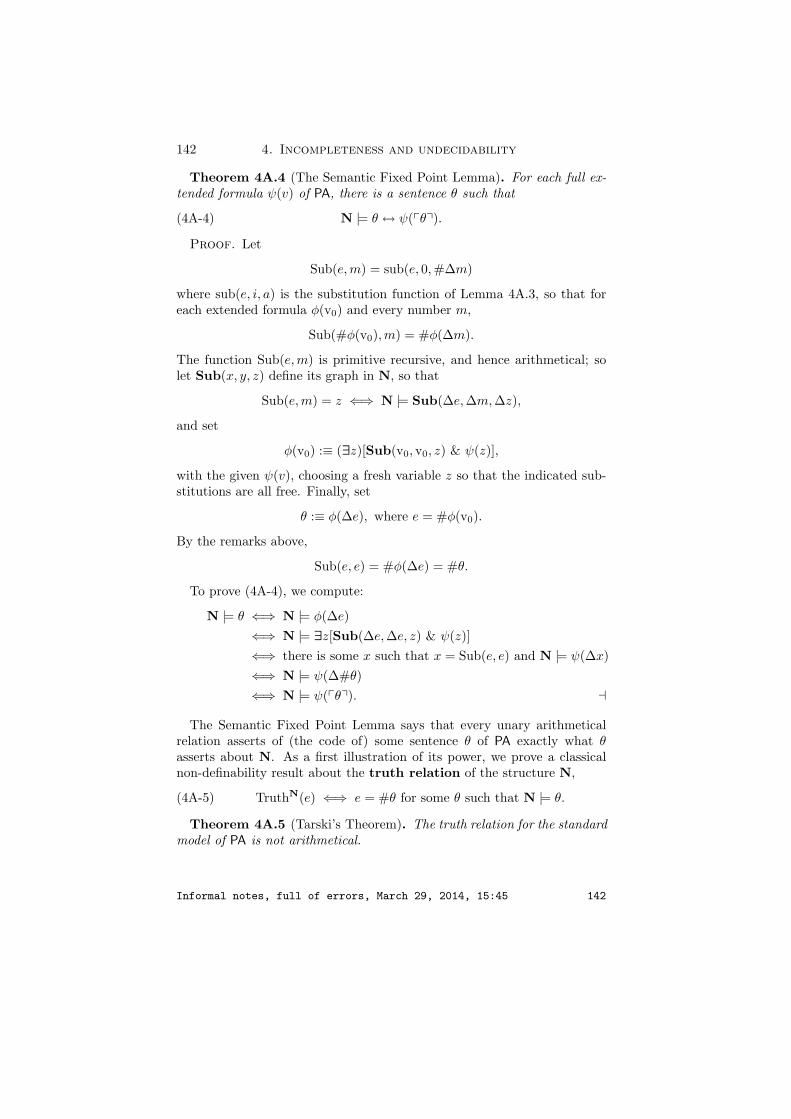
142 4. Incompleteness and undecidability
Theorem 4A.4 (The Semantic Fixed Point Lemma). For each full ex-tended formula ψ(v) of PA, there is a sentence θ such that
N |= θ ↔ ψ(pθq).(4A-4)
Proof. Let
Sub(e,m) = sub(e, 0, #∆m)
where sub(e, i, a) is the substitution function of Lemma 4A.3, so that foreach extended formula φ(v0) and every number m,
Sub(#φ(v0), m) = #φ(∆m).
The function Sub(e,m) is primitive recursive, and hence arithmetical; solet Sub(x, y, z) define its graph in N, so that
Sub(e,m) = z ⇐⇒ N |= Sub(∆e, ∆m,∆z),
and set
φ(v0) :≡ (∃z)[Sub(v0, v0, z) & ψ(z)],
with the given ψ(v), choosing a fresh variable z so that the indicated sub-stitutions are all free. Finally, set
θ :≡ φ(∆e), where e = #φ(v0).
By the remarks above,
Sub(e, e) = #φ(∆e) = #θ.
To prove (4A-4), we compute:
N |= θ ⇐⇒ N |= φ(∆e)⇐⇒ N |= ∃z[Sub(∆e,∆e, z) & ψ(z)]⇐⇒ there is some x such that x = Sub(e, e) and N |= ψ(∆x)⇐⇒ N |= ψ(∆#θ)⇐⇒ N |= ψ(pθq). a
The Semantic Fixed Point Lemma says that every unary arithmeticalrelation asserts of (the code of) some sentence θ of PA exactly what θasserts about N. As a first illustration of its power, we prove a classicalnon-definability result about the truth relation of the structure N,
TruthN(e) ⇐⇒ e = #θ for some θ such that N |= θ.(4A-5)
Theorem 4A.5 (Tarski’s Theorem). The truth relation for the standardmodel of PA is not arithmetical.
Informal notes, full of errors, March 29, 2014, 15:45 142

4A. Tarski and Godel (First Incompleteness Theorem) 143
Proof. If the truth relation were arithmetical, then its negation wouldalso be arithmetical, and so there would exist a full extended formula ψ(v)such that for every sentence θ of PA,
N 6|= θ ⇐⇒ ¬TruthN(#θ) ⇐⇒ N |= ψ(pθq).(4A-6)
By the Semantic Fixed Point Lemma, there is a sentence θ such that
N |= θ ⇐⇒ N |= ψ(pθq),
which is absurd, since with (4A-6) it implies that
N |= θ ⇐⇒ N 6|= θ. aTo derive incompleteness results about PA by this method, we need to
check that the provability relation of PA is arithmetical. We introduce theappropriate more general notions, which we will also need in the sequel.
Definition 4A.6 (Axiomatizations). Let T be a τ -theory, i.e., (by 1G.2)any set of sentences in FOL(τ).
A set of axioms for T is any set S of sentences of FOL(τ) such that forall θ,
S ` θ ⇐⇒ T ` θ;(4A-7)
T is finitely axiomatizable if it has a finite set of axioms; and T is(primitive recursively) axiomatizable if its signature τ is finite and T hasa set of axioms S which is primitive recursive (in the codes), i.e., such thatthe set of codes
#S = #θ | θ ∈ S(4A-8)
is primitive recursive.Notice that if a τ -theory is axiomatizable, then (by definition) τ is a
finite signature, and the codes in (4A-8) are computed relative to someenumeration s1, . . . , sk of the symbols in τ . Some results about axioma-tizable theories depend on the selection of a specific (primitive recursive)axiomatization, and in a few cases this is important; we will make sure toindicate these instances.
Note. In some books, by “theory” they mean a set T of sentences in alanguage which is closed under deducibility, i.e., such that
T ` θ =⇒ θ ∈ T (θ in the vocabulary of T ).
We have not done this here, and so we must be careful in understandingcorrectly results stated when this alternative usage is in effect.
Lemma 4A.7. Every finite theory is axiomatizable; PA is axiomatiz-able; and if T1 and T2 are both axiomatizable, then so is their union T1∪T2.(Cf. Problem x4.14.)
Informal notes, full of errors, March 29, 2014, 15:45 143

144 4. Incompleteness and undecidability
Definition 4A.8 (Proof predicates). We code the proofs of a theory Tas sequences of strings:
Proof T (e, y) ⇐⇒ e is the code of a formula φ
and y is the code of a proof of φ from T
⇐⇒ there exist formulas φ, φ1, . . . , φn−1 such thate = #φ and y = 〈#φ1, . . . , #φn−1, #φ〉and φ1, . . . , φn−1, φ is a proof of T .
It is simpler here to use proofs in the Hilbert-style proof system for FOLdefined in Section 1H, but we could use proofs in the Gentzen system withonly a minor complication in the codings.
Lemma 4A.9. If T is an axiomatizable theory, then its proof predicateProof T (e, y) (with respect to any primitive recursive axiomatization) isprimitive recursive. (Cf. Problem x4.15.)
Proof is tedious but basically trivial, because the axioms and the rulesof inference of first order logic can be checked“primitive recursively” in thecodes. a
Recall from Definition 1H.11 that a τ -theory T is complete if for eachτ -sentence θ,
either T ` θ or T ` ¬θ;
so T is incomplete if there is a τ -sentence θ such that
neither T ` θ nor T ` ¬θ.
A theory T in the language of arithmetic is sound if the standard modelN = (N, 0, S, +, ·) satisfies it, N |= T .
Theorem 4A.10 (Godel’s First Incompleteness Theorem). Every axiom-atizable, sound theory T in the language of arithmetic is incomplete.
In particular, PA is incomplete.
Proof. The proof predicate Proof T (e, y) constructed from a primitiverecursive axiomatization of T is primitive recursive, hence arithmetical, andso it is defined by some full extended formula Proof T (e, y). The SemanticFixed Point Lemma 4A.4 applied to the formula
ψ(v0) ≡ (∀y)¬Proof T (v0, y),
yields a sentence γT such that
N |= γT ⇐⇒ N |= (∀y)¬Proof T (pγT q, y),
Informal notes, full of errors, March 29, 2014, 15:45 144

4B. Numeralwise representability in Q 145
and we can compute, using properties of the satisfaction relation:
N |= γT ⇐⇒ N |= (∀y)¬Proof T (pγT q, y)⇐⇒ for every m,N |= ¬Proof T (pγT q, ∆m)⇐⇒ for every m,¬Proof T (#γT ,m)⇐⇒ T 6` γT .
It follows that N |= γT , since otherwise (by this equivalence) T ` γT —andthen γT is true by the soundness of T , and so it cannot be that T ` ¬γT ;and since N |= γT , by the same equivalence, T 6` γT . a
Notice that the Godel sentence γT depends on the specific axiomatiza-tion of T chosen for the proof; but the theorem—that T is incomplete—doesnot refer to any specific axiomatization of T , or to any particular methodof coding the syntactic objects of T . In applying the result to a specifictheory, e.g., PA, we do not even need to refer to the possibility of coding :we introduce a coding and check the axiomatizability of PA as part of theproof.
4B. Numeralwise representability in Q
Godel’s First Incompleteness Theorem 4A.10 applies only to sound theo-ries; and while this may appear to be not a serious limitation (because whowould be interested in theories which prove false number-theoretic facts),its extension to (all interesting) axiomatizable, consistent theories has, infact, many applications and reveals new and deeper limitations of first or-der axiomatic theories. To prove these results, we need to do some prooftheory.
Our aim in this section is to introduce the relevant notions and to showthat the axiomatic theory Q defined in 1G.11 is strong enough to provemany fundamental properties of primitive recursive functions and relations,even though it is otherwise very weak, cf. Problems x1.33 and x4.10. Usingthese facts, we will establish the Fixed Point Theorem 4B.14, a proof-theoretic version of Theorem 4A.4 which is the main tool for the strongerresults of Godel Theory.
Definition 4B.1. Let T be a theory in the language of PA. A fullextended formula F(v1, . . . , vn, y) numeralwise represents in T an n-ary function f : Nn → N, if for all x1, . . . , xn, w ∈ N,
f(x1, . . . , xn) = w =⇒ T ` F(∆x1, . . . , ∆xn,∆w)and T ` (∃!y)F(∆x1, . . . , ∆xn, y).
Informal notes, full of errors, March 29, 2014, 15:45 145
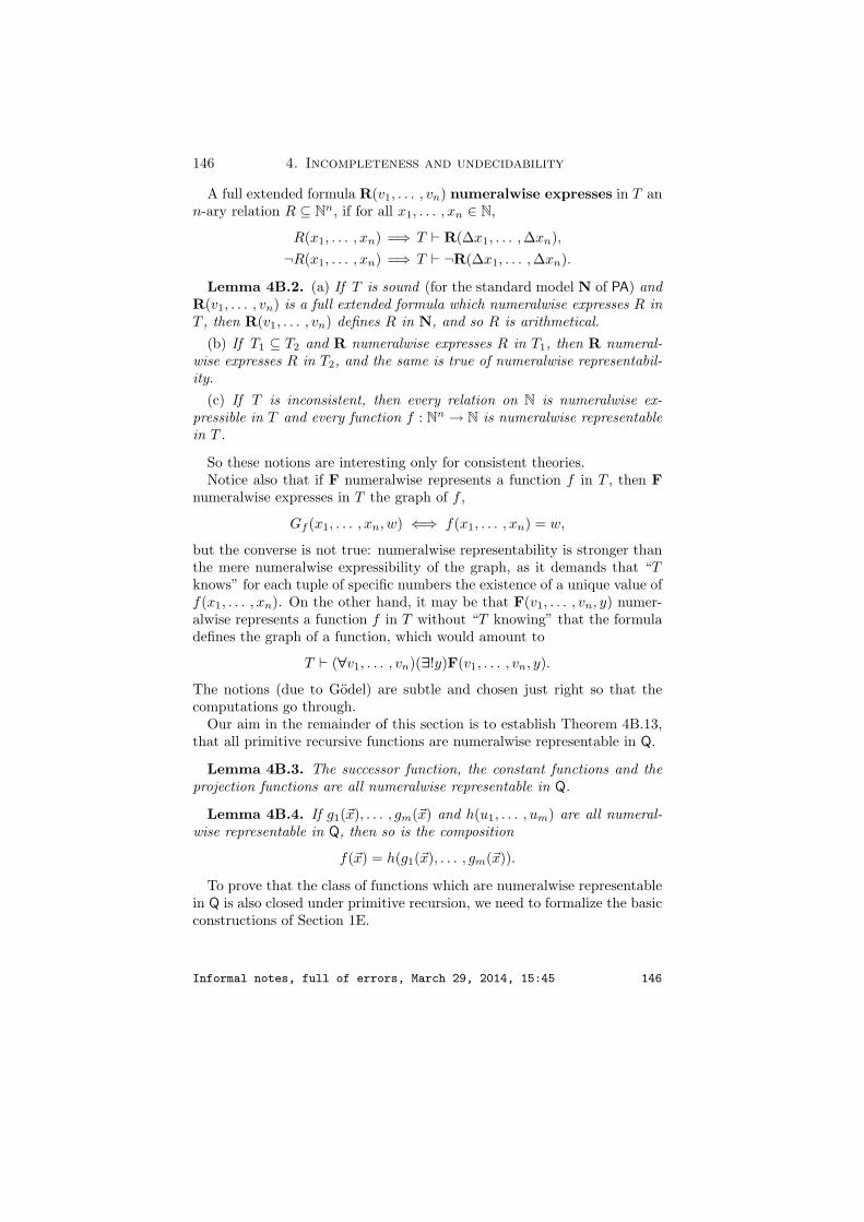
146 4. Incompleteness and undecidability
A full extended formula R(v1, . . . , vn) numeralwise expresses in T ann-ary relation R ⊆ Nn, if for all x1, . . . , xn ∈ N,
R(x1, . . . , xn) =⇒ T ` R(∆x1, . . . , ∆xn),¬R(x1, . . . , xn) =⇒ T ` ¬R(∆x1, . . . , ∆xn).
Lemma 4B.2. (a) If T is sound (for the standard model N of PA) andR(v1, . . . , vn) is a full extended formula which numeralwise expresses R inT , then R(v1, . . . , vn) defines R in N, and so R is arithmetical.
(b) If T1 ⊆ T2 and R numeralwise expresses R in T1, then R numeral-wise expresses R in T2, and the same is true of numeralwise representabil-ity.
(c) If T is inconsistent, then every relation on N is numeralwise ex-pressible in T and every function f : Nn → N is numeralwise representablein T .
So these notions are interesting only for consistent theories.Notice also that if F numeralwise represents a function f in T , then F
numeralwise expresses in T the graph of f ,
Gf (x1, . . . , xn, w) ⇐⇒ f(x1, . . . , xn) = w,
but the converse is not true: numeralwise representability is stronger thanthe mere numeralwise expressibility of the graph, as it demands that “Tknows” for each tuple of specific numbers the existence of a unique value off(x1, . . . , xn). On the other hand, it may be that F(v1, . . . , vn, y) numer-alwise represents a function f in T without “T knowing” that the formuladefines the graph of a function, which would amount to
T ` (∀v1, . . . , vn)(∃!y)F(v1, . . . , vn, y).
The notions (due to Godel) are subtle and chosen just right so that thecomputations go through.
Our aim in the remainder of this section is to establish Theorem 4B.13,that all primitive recursive functions are numeralwise representable in Q.
Lemma 4B.3. The successor function, the constant functions and theprojection functions are all numeralwise representable in Q.
Lemma 4B.4. If g1(~x), . . . , gm(~x) and h(u1, . . . , um) are all numeral-wise representable in Q, then so is the composition
f(~x) = h(g1(~x), . . . , gm(~x)).
To prove that the class of functions which are numeralwise representablein Q is also closed under primitive recursion, we need to formalize the basicconstructions of Section 1E.
Informal notes, full of errors, March 29, 2014, 15:45 146

4B. Numeralwise representability in Q 147
Definition 4B.5. We introduce the formal abbreviations
x ≤ y ≡ (∃z)[z + x = y],x < y ≡ x ≤ y & ¬(x = y),
(∃u ≤ y)φ ≡ (∃u)[u ≤ y & φ],(∀u ≤ y)φ ≡ (∀u)[u ≤ y → φ].
The use of z + x rather than x + z in the definition of x ≤ y is important,because (as we have shown) Q cannot prove the commutativity of addition.
Lemma 4B.6. Q can prove all true propositional combinations of closedequalities and inequalities between terms; i.e., if θ is a propositional sen-tence in the signature (0, S,+, ·,≤), then
N |= θ ⇐⇒ Q ` θ.
(Cf. Problem x4.10∗.)
Proof. Check first by structural induction, that for each closed term tin the language of arithmetic, if value(t) = n, then Q ` t = ∆n, and thenprove by structural induction that for every quantifier free sentence θ,
N |= θ ⇐⇒ Q ` θ and N |= ¬θ ⇐⇒ Q ` ¬θ. a
Lemma 4B.7. Q ` (∀x)[x ≤ ∆m → x = ∆0∨ x = ∆1∨ · · · ∨ x = ∆m].As a consequence,
Q, φ(∆0), . . . , φ(∆m) ` (∀u ≤ ∆m)φ(u).
(Q knows all the predecessors of a numeral and can quantify over the initialsegment below a numeral.)
Proof is by induction on the number m. aLemma 4B.8. The remainder function rem(x, y) is numeralwise repre-
sentable in Q, and hence so is the Godel β-function
β(c, d, i) = rem(c, 1 + (i + 1)d).
Lemma 4B.9. For every m ∈ N,
Q ` S(z) + ∆m = z + S(∆m).
Proof is by induction on m. aLemma 4B.10. For m ∈ N,
Q ` (∀x)[x ≤ ∆m ∨∆(m + 1) ≤ x].
Proof is by induction on m. a
Informal notes, full of errors, March 29, 2014, 15:45 147

148 4. Incompleteness and undecidability
Lemma 4B.11. If f(x1, . . . , xn) is numeralwise representable in Q, thenthere exists a full extended formula F(v1, . . . , vn, y) such that the followinghold for all numbers x1, . . . , xn, w:
1. f(x1, . . . , xn) = w =⇒Q ` F(∆x1, . . . , ∆xn,∆w).2. Q,F(v1, . . . , vn,∆w),F(v1, . . . , vn, y) ` y = ∆w.
In particular, F(v1, . . . , vn, y) numeralwise represents f (in a very strongway).
Proof. Let F1(v1, . . . , vn, y) numeralwise represent f , and take
F(v1, . . . , vn, y) ≡ F1(v1, . . . , vn, y) & (∀u < y)¬F1(v1, . . . , vn, u),
where u < y abbreviates u ≤ y & u 6= y. aLemma 4B.12. If f is defined by the primitive recursion
f(0, ~x) = g(~x), f(t + 1, ~x) = h(f(t, ~x), t, ~x)
and g, h are numeralwise representable in Q, then so is f ; and the sameholds for primitive recursion without parameters (1E-5).
Proof. We start with Dedekind’s analysis of the primitive recursivedefinition,
f(t, ~x) = w ⇐⇒ there exists a sequence (w0, . . . , wt) such that
w0 = g(~x) & (∀s < t)[ws+1 = h(ws, s, ~x)] & w = wt;
we then choose formulas B(c, d, i, y), G(~x, u) and H(u, t, ~x,w) which nu-meralwise represent the β-function, g and h in the strong sense of thepreceding Lemma; and we set
F(t, ~x, w) ≡ [t = 0 & G(~x,w)]∨(∃c)(∃d)[(∃q)[G(~x,w) & B(c, d, 0, q)]
& (∀i < t)(∀u)(∀v)[[B(c, d, i, u) & H(u, ~x, i, v)]→ B(c, d, S(i), v)]
& B(c, d, i, w)]. aTheorem 4B.13. Every primitive recursive function is numeralwise rep-
resentable in Q; and every primitive recursive relation is numeralwise ex-pressible in Q.
Proof. For the second assertion, let F(~v, y) numeralwise represent thecharacteristic function of R and set
R(~v) ≡ F(~v, 1);
proof that this formula numeralwise expresses R follows from the assump-tion that for all x1, . . . , xn,
Q ` (∃!y)F(∆x1, . . . , ∆xn, y). a
Informal notes, full of errors, March 29, 2014, 15:45 148

4B. Numeralwise representability in Q 149
It is important for the applications, to notice that the next, basic resultapplies to theories in the language of PA which need not be sound for thestandard model N.
Theorem 4B.14 (The Fixed Point Lemma). If T is a theory in thelanguage of arithmetic which extends Robinson’s system Q, then for eachfull extended formula ψ(v), we can find a sentence θ such that
T ` θ ↔ ψ(pθq).(4B-1)
Proof. As in the proof of Theorem 4A.4, let
Sub(e,m) = sub(e, 0, #∆m)
where sub(e, i, a) is the substitution function of the Substitution Lemma 4A.3,so that for each extended formula φ(v0),
Sub(#φ(v0), m) = #φ(∆m).
The function Sub(e,m) is primitive recursive; so let Sub(x, y, z) numeral-wise represent it in T (and such that v0 does not occur in it), and set
φ(v0) :≡ (∃z)[Sub(v0, v0, z) & ψ(z)],
choosing again a fresh variable z, so that the indicated substitutions are allfree. Set
θ :≡ φ(∆e), where e = #φ(v0),
so that by the remark above,
Sub(e, e) = #φ(∆e) = #θ.
From the definition of numeralwise representability (and the definition ofpθq = ∆#θ), we have
T ` Sub(∆e,∆e, pθq),(4B-2)
and T ` (∀z)[Sub(∆e, ∆e, z) → z = pθq].(4B-3)
To prove (4B-1), argue in T as follows: if ψ(pθq), we have
Sub(∆e, ∆e, pθq) & ψ(pθq)
from (4B-2), which yields
(∃z)[Sub(∆e, ∆e, z) & ψ(z)],
i.e., φ(∆e), i.e., θ; and if θ, we have
(∃z)[Sub(∆e, ∆e, z) & ψ(z)],
which with (4B-3) yields ψ(pθq), and completes the proof. a
Informal notes, full of errors, March 29, 2014, 15:45 149

150 4. Incompleteness and undecidability
4C. Rosser, more Godel and Lob
If T1, T2 are theories in the same language FOL(τ), we (naturally) saythat
T1 is weaker than T2 and T2 is stronger than T1
⇐⇒ for all τ -sentences θ, T1 ` θ =⇒T2 ` θ;
the next definition extends this idea in a natural way to theories in differentlanguages.
4C.1. Interpretations. Let T1, T2 be theories, in two (possibly differ-ent) languages FOL(τ1), FOL(τ2) of finite signatures. A (propositionallyfaithful, minimal) interpretation of T1 in T2 is a primitive recursive func-tion π from the sentences of T1 to sentences of T2 such that the followinghold.(1) T1 ` θ =⇒T2 ` π(θ).(2) T2 ` π(¬θ) ↔ ¬π(θ).(3) T2 ` π(φ & ψ) ↔ π(φ) & π(ψ).
Here we call π : Sentences(T1) → Sentences(T2) primitive recursive if thereis a primitive recursive function π∗ : N→ N such that
#π(φ) = π∗(#φ) (φ any sentence of T1),
where # denotes the coding function of FOL(τ2) on the left and the codingfunction of FOL(τ1) on the right. Notice that (2) and (3) together implythat an interpretation preserves the propositional structure of sentences,for example
T2 ` π(φ → ψ) ↔ (π(φ) → π(ψ)).
Directly from the definition, we get:
Lemma 4C.2. If T ′1 is weaker than T1, T2 is weaker than T ′2, and πinterprets T1 in T2, then π interprets T ′1 in T ′2.
When T2 = T1 or the language of T2 is the same (or an expansion) ofthe language of T1 and T2 has more axioms, then the identity functioninterprets T1 in T2. For an example of an interpretation between entirelydifferent languages, we note (without proof) the classical interpretation ofPeano arithmetic in the axiomatic set theories specified in Definition 1G.12,which is constructed by “defining” the natural numbers within set theory:
Proposition 4C.3. Peano arithmetic PA is interpretable in Zermelo’sset theory without choice Z, and hence every subtheory of PA is interpretablein all the (stronger) axiomatic set theories listed in Definition 1G.12.
Informal notes, full of errors, March 29, 2014, 15:45 150

4C. Rosser, more Godel and Lob 151
Much stronger notions of interpretation exist and are often useful, butthis is all we need now; and for the theorems we will prove, the weaker thenotion of interpretation employed, the better.
Theorem 4C.4 (Rosser’s form of Godel’s First Theorem). If T is a con-sistent, axiomatizable theory and Q is interpretable in T , then T is incom-plete.
Proof. Fix an interpretation π of Q in T , set
Proof π,T (e, y) ⇐⇒ e codes a sentence φ of PA
and y codes a proof in T of the translation π(φ),Refuteπ,T (e, y) ⇐⇒ e codes a sentence φ of PA
and y codes a proof in T of the translation π(¬φ),
and let Proof π,T (e, y), Refuteπ,T (e, y) be formulas of number theorywhich numeralwise express in Q these primitive recursive relations. Bythe Fixed Point Lemma for Q, we can construct a sentence
ρ = ρ(T, π)
in the language of PA, such that
Q ` ρ ↔ (∀y)[Proof π,T (pρq, y) → (∃u ≤ y)Refuteπ,T (pρq, u)].(4C-4)
The Rosser sentence ρ expresses the unprovability of its translation in T ,but in a round-about way: it asserts that “for each one of my proofs, thereis a shorter (not longer) proof of my negation”.
(a) Suppose towards a contradiction that there is a proof of πρ in T ,with code m, so by the hypotheses,
Q ` Proof π,T (pρq, ∆m).
Taking y = ∆m and appealing to the hypothesis and basic facts about Q,we get that
Q ` (∃y)[Proof π,T (pρq, y) & (∀u ≤ y)¬Refuteπ,T (pρq, u)];
thus with (4C-4), Q ` ¬ρ, hence T ` π(¬ρ), i.e., T ` ¬π(ρ), contradictingthe assumed consistency of T .
(b) Suppose now that there is a proof in T of ¬π(ρ), hence a proof ofπ(¬ρ), and let m be its code. We know that
Q ` Refuteπ,T (pρq, ∆m),
among other things. To prove
(∀y)[Proof π,T (pρq, y) → (∃u ≤ y)RefuteπT (pρq, u)](4C-5)
in Q, we take cases (by Lemma 4B.10) on whether
y ≤ ∆m ∨∆(m + 1) ≤ y;
Informal notes, full of errors, March 29, 2014, 15:45 151

152 4. Incompleteness and undecidability
in the first of these cases we know (by Lemma 4B.7, in Q) that y = ifor some i ≤ m, and it is trivial to verify that ¬Proof π,T (pρq, y), sincethis sentence is true and Q knows such true assertions about the values ofProof π,T by Lemma 4B.6. In the second case, Q knows ∆m ≤ y, in whichcase the conclusion of the implication in (4C-5) follows immediately. So wehave proved (4C-5) which is equivalent in Q to ρ by (4C-4), contradicting(a). a
Notice (again) that the Rosser sentence ρ we constructed depends ona specific axiomatization of T chosen for the proof, as well as a specificinterpretation of Q into T ; but the result—the incompleteness of T—isindependent of these parameters, and for specific theories T , we can incor-porate the verification of axiomatizability in the proof and derive a resultwhich is entirely independent of any particular coding. This is certainlythe case for the axiomatic theories of Definition 1G.12, for which the resultis very clean, e.g., if ZFC is consistent, then it is incomplete.
4C.5. Remarks. Rosser’s form of Godel’s Theorem 4C.4 is much moregeneral than Godel’s First Incompleteness Theorem 4A.10, as it does notmake any soundness assumptions of T : it applies, for example, to the theoryPA +¬γPA, which is consistent but certainly not sound, cf. Problem x4.16.It also applies to axiomatic set theories, for which it is easy to establishthat they interpret Q, but it is not clear exactly in what sense they aresound, and (in some cases) it is not even completely clear that they areconsistent!
Next we identify a specific, especially interesting fact that sufficientlystrong, consistent theories can express but cannot prove:
Definition 4C.6. For each axiomatizable theory T , let
ConsisT ≡ ¬(∃e)(∃u)(∃v)[Proof T (e, u) & RefuteT (e, v)];
this is the sentence of number theory which expresses formally the consis-tency of T—with respect, again, to a specific axiomatization of T .
Lemma 4C.7. If T is axiomatizable and consistent, π is an interpre-tation of Q in T , and ρT is the Rosser sentence of T for π, then
PA ` ConsisT → ρT .
Proof. The proof of (a) Theorem 4C.4 is elementary, and it can beformalized in Peano Arithmetic; thus
PA ` ConsisT → (∀y)¬Proof T (pρT q, y).
On the other hand, ρT expresses precisely its unprovability, albeit in around-about way, but still,
PA ` ρT ↔ (∀y)¬Proof (pρT q, y);
Informal notes, full of errors, March 29, 2014, 15:45 152

4C. Rosser, more Godel and Lob 153
and these two claims, together, yield the Lemma. aTheorem 4C.8 (Godel’s Second Incompleteness Theorem). If T is an
axiomatizable, consistent theory such that PA is interpretable into it bysome function π, then πConsisT is not a theorem of T .
In particular, PA cannot prove its own consistency, unless it is inconsis-tent.
Proof is immediate from the Lemma, since T 6` πρT . aFor any sentence θ in the language of PA, clearly
N |= (∃y)Proof PA(pθq, y) → θ;(4C-6)
this is just a formal expression of the soundness of PA. It should be that PAcan prove this basic principle—recognize that it is sound—but it cannot,except when it is trivial:
Theorem 4C.9 (Lob’s Theorem). For each sentence θ of number the-ory,
if PA ` (∃y)Proof PA(pθq, y) → θ, then PA ` θ.
Proof. Towards a contradiction, we assume that
PA ` (∃y)Proof PA(pθq, y) → θ but PA 6` θ
for some θ, so that the theory
T = PA ∪ ¬θis consistent. We now argue (in outline) that some metamathematicalarguments can be formalized in PA, to infer that T ` ConsisT , contraryto the Second Incompleteness Theorem for T .
From the hypothesis,
PA ` ¬θ → ¬(∃y)Proof PA(pθq, y),
so that
T ` ¬(∃y)Proof PA(pθq, y).
Next we claim that
PA ` (∃y)Proof T (p0 = 1q, y) ↔ (∃y)Proof PA(p¬θ → (0 = 1)q, y),
i.e., that PA recognizes (in effect) the Deduction Theorem; and also that
PA ` (∃y)Proof PA(p¬θ → (0 = 1)q, y) ↔ (∃y)Proof PA(pθq, y),
i.e., that PA recognizes that it can do proofs by contradiction. ReplacingPA by the stronger T and combining these two equivalences, we get
T ` ¬(∃y)Proof T (p0 = 1q, y) ↔ ¬(∃y)Proof PA(pθq, y);
and since T proves the right-hand-side of this equivalence, it also provesthe left-hand-side, which implies (in PA) ConsisT . a
Informal notes, full of errors, March 29, 2014, 15:45 153

154 4. Incompleteness and undecidability
It should be clear that the appropriate version of Lob’s Theorem holdsfor any consistent, axiomatizable theory T in which PA can be interpreted,cf. Problem x4.18∗.
4C.10. Provability theory. It is convenient to introduce a notationfor the sentences which express formally provability, and so for a fixedaxiomatizable T in the language of PA and any sentence θ, we set:
¤T (θ) :≡ (∃y)Proof T (pθq, y).(4C-7)
This sentence depends, of course, on the specific axiomatization of T wechoose to define the proof predicate.
With this notation, Lob’s Theorem takes the simple form
if PA ` ¤PA(θ) → θ, then PA ` θ,
and the question arises whether its formal version can be proved in PA, i.e.,whether the following holds for each sentence θ:
PA ` ¤PA(¤PA(θ) → θ) → ¤PA(θ).
This is indeed true, and has interesting consequences. To show it, we mustlook a little more carefully at how various informal (mathematical) claimscan be formalized and proved in axiomatized theories, a topic which isgenerally referred to as provability theory. We will confine ourselves hereto just a few, basic facts.
4C.11. Bounded and Σ1 formulas. A formula φ in the language ofPA is bounded if it contains only bounded quantifiers as in Definition 4B.5,i.e., more precisely, if it belongs to the smallest set of formulas which con-tains all the prime formulas of the form s = t and is closed under thepropositional connectives and bounded quantification, i.e., the formationrules
ψ 7→ (∃vi ≤ vj)ψ, ψ 7→ (∀vi ≤ vj)ψ.
A formula φ is Σ1 if
φ ≡ ∃x1 · · ·∃xnψ
where ψ is a bounded formula.For any theory T in the language of PA, a formula φ is T -bounded or
T -Σ1 if there is a bounded or Σ1 formula φ∗ such that
T ` φ ↔ φ∗;
and a formula φ is T -∆1, if both φ and ¬φ are T -Σ1.
Proposition 4C.12. Suppose T is an extension of PA, in the languageof PA.
Informal notes, full of errors, March 29, 2014, 15:45 154

4C. Rosser, more Godel and Lob 155
(1) The class of T -Σ1 formulas includes all prime formulas and is closedunder the positive propositional connectives & and ∨, bounded quantifica-tion of both kinds, and unbounded existential quantification.
(2) For each primitive recursive function f(~x), there is a T -∆1 formulaφ(~v, w) which numeralwise represents f(~x) in T .
(3) Each primitive recursive relation is numeralwise expressible in T bya T -∆1 formula.
Proof of these propositions can be extracted by reading with some carethe proofs in Section 4B, and formalizing in the given T some easy, informalarguments. For example, to show for the proof of (1) that the class of T -Σ1
formulas is closed under universal bounded quantification, it is enough toshow that for any extended formula φ(x, y, z),
T ` (∀x ≤ y)(∃z)φ(x, y, z) ↔ (∃w)(∀x ≤ y)(∃z ≤ w)φ(x, y, z);
the equivalence expresses an obvious fact about numbers, which can beeasily proved by induction on y—and this induction can certainly be for-malized in PA.
(2) and (3) can be read-off the proof of the basic Theorem 4B.13, bycomputing the forms of all the formulas used in that proof and appealingto (1) of this Proposition. a
Proposition 4C.13. Suppose T is an axiomatizable extension of PA,in the language of PA.
(1) The proof predicate Proof T (e, y) of T is numeralwise expressible by aT -∆1 formula Proof T (e, y); and hence, for each sentence θ, the provabilityassertion ¤T (θ) is a T -Σ1 sentence.
(2) For every T -Σ1 sentence φ,
T ` φ → ¤T (φ).
(3) For every sentence θ,
T ` ¤T (θ) → ¤T (¤T (θ)).
Proof. (1) The formula Proof T (e, y) is T -∆1 by (3) of the precedingtheorem, and so ¤T (θ) is T -Σ1 by its definition (4C-7).
(2) Notice that this is not a trivial claim, because it does not, in general,hold for sentences which are not T -Σ1: if, for example, T is sound and γT
is its Godel sentence, then γT → ¤T (γT ) is not true, and so it is not atheorem of T . To prove the claim, let
Proof nT (e, x1, . . . , xn, y) ⇐⇒ e is the code of
a full extended formula φ(v1, . . . , vn)
and y is the code of a proof of φ(∆x1, . . . , ∆xn) from T .
Informal notes, full of errors, March 29, 2014, 15:45 155

156 4. Incompleteness and undecidability
This is a generalization of the proof relation Proof T (e, y), so that, in fact
Proof T (e, y) ⇐⇒ Proof 0T (e, y),
and it is also primitive recursive. Let Proof nT (x0, x1, . . . , xn, y) be a
formula which numeralwise expresses Proof nT (e, x1, . . . , xn, y) in T . The
heart of the proof is to show that for every full extended bounded formulaψ(v1, . . . , vn),
T ` ψ(x1, . . . , xn) → (∃y)Proof nT (pψ(x1, . . . , xn)q, x1, . . . , xn, y).
(4C-8)
This is verified by induction on the construction of bounded formulas, i.e.,it is shown first for prime formulas, and then it is shown that it persistsunder the positive propositional connectives and bounded quantification.Notice, again, that a detailed (complete) proof would involve a good dealof work: for example, to show (part of) the basic case
T ` u + v = w → (∃y)Proof 3T (pu + v = wq, u, v, w, y),(4C-9)
we must formalize in T the informal claim
if u + v = w, then T ` ∆u + ∆v = ∆w;
the proof of the informal claim is by induction on v—and so the formalproof of (4C-9) requires induction within T . This is why we assume in thetheorem that T extends PA—there is no way to show this result for weaktheories like Q. On the other hand, PA is a powerful theory in which we canformalize inductive proofs, and so (4C-8) is plausible, and can be verifiedwith some computation.
To complete the proof of (2), suppose
φ ≡ (∃x1) · · · (∃xn)ψ(x1, . . . , xn)
is a Σ1 sentence with ψ(x1, . . . , xn) bounded and having no free variablesother than the indicated x1, . . . , xn, and argue in T . Assume ψ(x1, . . . , xn),and infer
(∃y)Proof nT (pψ(x1, . . . , xn)q, x1, . . . , xn, y)
by (4C-8). From this, by trivial properties of the provability relations(which can be formally established in PA), infer that
(∃y)Proof (p(∃x1) · · · (∃xn)ψ(x1, . . . , xn)q, y).
So we have shown that
T ` ψ(x1, . . . , xn) → (∃y)Proof (p(∃x1) · · · (∃xn)ψ(x1, . . . , xn)q, y),
from which we get immediately the required
T ` (∃x1) · · · (∃xn)ψ(x1, . . . , xn)
→ (∃y)Proof (p(∃x1) · · · (∃xn)ψ(x1, . . . , xn)q, y).
Informal notes, full of errors, March 29, 2014, 15:45 156

4D. Computability and undecidability 157
Finally, (3) follows from (1) and (2). aBy methods like these, we can show that the statement and proof of Lob’s
Theorem for any axiomatizable extension of PA, can also be formalized inPA:
Theorem 4C.14. For any axiomatizable extension T of PA, and everysentence θ,
PA ` ¤T (¤T (θ) → θ) → ¤T (θ).
The most complex part of the argument is the formalization in PA of theproof of the Second Incompleteness Theorem of Godel 4C.8.
And, finally, to prove the following considerably deeper result, we alsoneed to formalize in PA the Gentzen Hauptsatz:
Theorem 4C.15. PA is not finitely axiomatizable.
This is somewhat different from the preceding is that its statement (asopposed to its proof) does not depend on any particular coding of formulas,proofs, etc.: the result simple asserts that no finite set of sentences in thelanguage of PA has exactly the same consequences as PA.
4D. Computability and undecidability
Is it possible to determine “effectively” whether an arbitrary sentence ofarithmetic is true? Godel’s First Incompleteness Theorem shows that thiscannot be done by the classical axiomatic method, i.e., by singling out some“obvious” arithmetical truths and then (formally) proving all the others,but it may be argued that this exhibits only a fundamental incompletenessof the axiomatic method : it may be that some other method (unrelated tologic) might “identify” effectively all arithmetical truths, without necessar-ily justifying them (by reducing them to some few, obvious axioms). Wewill show in this and the next two sections that this cannot be done, byproving that there is no general method which can decide effectively whethera given sentence of the language of arithmetic is true. The methods we willuse (due to Turing, Church and Kleene) will yield a host of related unde-cidability results which are among the most fundamental applications oflogic.
For each set Λ of “symbols”, Λ∗ is the set of strings (words, finite se-quences) from Λ, including the empty string ε. For example, the sets ofterms and formulas of FOL(τ) for a specific finite signature τ are sets ofstrings from the alphabet
¬ → & ∨ ∀ ∃ = ( ) , s1 . . . sk v0 v1 . . .
Informal notes, full of errors, March 29, 2014, 15:45 157

158 4. Incompleteness and undecidability
of FOL(τ). We can replace this by the finite alphabet
Vτ = ¬,→, & ,∨, ∀, ∃, =, (, ), , , s1, . . . sk, v, |where v (for “variable”) and the tally | are new symbols and we identifythe variable vi with the string of v followed by i + 1 tallies,
v0 ≡ v|, v1 ≡ v||, v2 ≡ v|||, . . .If we further think of proofs in FOL(τ) as sequences of formulas separatedby commas, then proofs are also words in this finite alphabet Vτ , i.e.,members of Vτ
∗. Thus the notion that we need to make precise is that ofa computable function
f : Λ∗ → Λ∗
for an arbitrary finite Λ; a set of words A ⊆ Λ∗ will be decidable if itscharacteristic function
χA(α) =
T if α ∈ A
F otherwise,
where T and F are any two, specific, distinct strings standing for truth andfalsity.
Alan Turing had (in 1936) the fundamental intuition that a string func-tion is computable if its values can be computed by some “mechanicaldevice” (machine) which has access to the string argument of the functionand an unbounded amount of “scratch paper” for each computation. Tur-ing’s abstract, mathematical model of “machine” was introduced beforeactual computers had been built, but it has proved very robust and (in allinteresting aspects other than efficiency, which does not concern us here)equivalent to the electronic computers we use today.
4D.1. Turing machines. A Turing machine is a structure
M = (S,Q0,Σ, Ã, Table),
where the following hold.(1) S is a finite set, the set of (internal) states of M , and Q0 ∈ S is a
specified initial state.(2) Σ is a finite set, the set of symbols (alphabet) of M , and à ∈ Σ is
a specified member of Σ standing for “the blank symbol” (empty space).(3) The Table of M is a finite set of transitions, i.,e., quintuples of the
form
Q,X 7→ X ′, Q′,m(4D-10)
where Q and Q′ are states; X and X ′ are symbols; and the move of thetransition m ∈ 0,−1,+1. We say that the pair (Q,X) activates thetransition.
Informal notes, full of errors, March 29, 2014, 15:45 158

4D. Computability and undecidability 159
A machine M is deterministic if for each state Q and each symbolX there is at most one transition which is activated by the pair (Q,X),otherwise it is non-deterministic.
Turing’s image is that the machine is situated in front of a two-wayinfinite tape which has a finite number of symbols from the alphabet placedon it; the machine can only see the symbol on the cell just in front of it—itcannot see any other symbols and it cannot see the coordinate of that cell,i.e., it does not “know” where it is on the tape.
( ∀ x ) R ( x à 3 Ã
−1 0 1 2 3 4
Q
6
If the machine is in state Q and the visible symbol is X, then each transi-tion (4D-10) in the machine’s Table which is activated by the pair (Q,X)produces a change in this situation, overwriting the symbol X by the newsymbol X ′, changing from the current state Q to the new state Q′ andmoving one-cell-to-the-left if the move m = −1, not-at-all if m = 0, andone-cell-to-the-right if m = 1. For example, the transition
Q, ) 7→ (, Q′, +1
will change the situation in the picture above to the new situation:
( ∀ x ( R ( x à 3 Ã
Q′
6
−1 0 1 2 3 4
Finally, a computation of M is a sequence of successive situations producedby transitions of M in this way, starting with an initial situation involvingthe initial state Q0.
Without further explanation of this simple idea, we proceed to the precisedefinitions of the notions italicized in these remarks.
Informal notes, full of errors, March 29, 2014, 15:45 159

160 4. Incompleteness and undecidability
Definition 4D.2. For a fixed Turing machine M = (S, Q0, Σ, Ã,Table),we define:
(1) A tape (description) is any function τ : Z → Σ, which assigns asymbol of M to each rational integer
i ∈ Z = . . . ,−3,−2,−1, 0, 1, 2, 3, . . . ,such that for all but finitely many i, τ(i) = Ã.
(2) A situation of M is any triple
s = (Q, τ, i),
where Q is a state, τ is a tape and i ∈ Z. The state of M in this situationis Q; the place of M in s is the integer i; and the visible symbol in s is τ(i).We call s initial if Q is the initial state Q0 of M and i = 0; and we call sterminal if either there is no transition in the table of M activated by thepair (Q, τ(i)) or the only transition activated by this pair is a “stand-pat”transition
Q,X 7→ X, Q, 0.
(3) A situation s′ = (Q′, τ ′, i′) is a next situation to s = (Q, τ, i) if s isnot terminal, if
j 6= i =⇒ τ(j) = τ ′(j),
and if the Table of M contains the transition
Q, τ(i) 7→ τ ′(i), Q′, i′ − i.
Notice that this implies |i′ − i| ≤ 1, since i′ − i is a move; that (by thedefinition) there is no s′ next to s if s is terminal; and that if M is deter-ministic, then there is at most one s′ next to s, since at most one transitioncan be activated by the given pair (Q, τ(i)).
(4) A computation of M is any (finite or infinite) sequence of situations
s0, s1, . . . ,
such that s0 is initial and each si+1 is next to si, diagrammatically
s0 7→ s1 7→ s2 7→ · · ·A computation is maximal if no extension of it is a computation, and amaximal, finite computation is called convergent. For each initial situations0, we set
(4D-11) M : s0↓⇐⇒ there exists a convergent computation s0 7→ · · · 7→ sm
and we read “M : s0↓” as “M halts” (or converges) on s0.
Informal notes, full of errors, March 29, 2014, 15:45 160

4D. Computability and undecidability 161
It follows easily that if M is deterministic, then for each initial situations0 = (Q0, τ, 0) there is exactly one maximal computation which starts withs0, and that a maximal computation is either finite, ending with a terminalsituation, or infinite (and with no terminal situations in it). We picturethese possibilities in the following, simple examples of Turing machines.
4D.3. Example. The machine with just one state Q0 on the alphabet1, Ã and just two transitions
Q0, 1 7→ 1, Q0, +1Q0, Ã 7→ 1, Q0, +1
is deterministic, and starting from any initial situation, it moves to theright forever, printing a 1 on every cell to the right of the origin which doesnot already have a 1 in it.
4D.4. Example. On the same alphabet 1, Ã, consider the machinewith the following transitions (and the states which occur in these transi-tions):
Q0, 1 7→ 1, Q0, +1(a)
Q0, Ã 7→ 1, Q1, 0(b)
Q1, 1 7→ 1, Q1,−1(c)
Q1, Ã 7→ Ã, Q2, +1(d)
For each number x, let
in(x) = · · · ÃÃ 11 . . . 1︸ ︷︷ ︸x+1
, ÃÃ . . .
be the tape with x + 1 1s on and to the right of the origin and no othersymbols but blanks, and consider the computation of this deterministicmachine starting with the initial situation (Q0, in(x), 0). It will start withx + 1 executions of the transition (a), as long at is sees a 1, and thenexecute (b) just once, to write a 1 on the first blank cell on the right; itwill then execute (c) x + 3 times, until it is back to the left of the origin,where it finds the first blank on the left, and finally execute (d) just onceto move to the origin and stop, in the situation (Q2, in(x + 1), 0).
For each string α ≡ α0α1 · · ·αn−1 ∈ Λ∗, let
in(α)(i) =
αi, if 0 ≤ i < n,
Ã, otherwise;
this is the tape that we use to represent a string α an an input to a compu-tation by a Turing machine whose alphabet includes Λ. Similarly, for each
Informal notes, full of errors, March 29, 2014, 15:45 161

162 4. Incompleteness and undecidability
tape τ , let
out(τ) =τ(0)τ(1) · · · τ(m− 1)
for the least m ∈ N such that τ(m) = Ã,
so that if τ(0) = Ã, then out(τ) = ε (the empty string), and if τ(0) = N ,τ(1) = O and τ(2) = Ã, then out(τ) = NO.
Definition 4D.5 (Turing computable functions). A Turing machine
M = (S, Q0, Σ, Ã,Table)
computes a functionf : Λ∗ → Λ∗
if Λ ⊆ Σ; Ã /∈ Λ; and for all strings α, β ∈ Λ∗,
f(α) = β ⇐⇒ there exists a convergent computation s0, s1, . . . sm of M
such that s0 = (Q0, in(α), 0) and sm = (Q, τ ′, i), with out(τ ′) = β.
Similarly, and representing each tuple x1, . . . , xn of numbers by the stringof 1s and blanks
in(x1, . . . , xn) = . . . ÃÃ 11 . . . 1︸ ︷︷ ︸x1+1
à 11 . . . 1︸ ︷︷ ︸x2+1
. . . Ã 11 . . . 1︸ ︷︷ ︸xn+1
ÃÃ . . .
(with in(x1, . . . , xn)(0) = the first 1), a Turing machine M as above com-putes a function
f : Nn → Nif the alphabet of M includes the symbol 1 and for all x1, . . . , xn, w,
f(x1, . . . , xn) = w ⇐⇒ there exists a convergent computations0, s1, . . . sm of Msuch that
s0 = (Q0, in(x1, . . . , xn), 0)
and sm = (Q, τ ′, i), with out(τ ′) = 11 . . . 1︸ ︷︷ ︸w+1
.
Note that in both situations, if the machine M is deterministic, thenfor each input, there will be exactly one convergent computation (“thecomputation”) of M which computes the value of the function.
A string or number-theoretic function is Turing computable if it iscomputed by a deterministic Turing machine.
After giving these definitions, Turing claimed that his simple, restrictedmachines can actually compute all functions on strings which are “intu-itively computable”, so that his precise definition can be used to prove rig-orously that specific functions are not computable in any way whatsoever,by showing that they cannot be computed by a Turing machine. AlonzoChurch had made a similar proposal for another, precisely defined class of
Informal notes, full of errors, March 29, 2014, 15:45 162

4D. Computability and undecidability 163
functions (subsequently proved to coincide with the class of Turing com-putable functions), so that the next, fundamental claim carries now boththeir names:
4D.6. The Church-Turing Thesis. A string function f : Λ∗ → Λ∗
(on a finite alphabet Λ) is computable exactly when it is Turing computable;and a set of strings A ⊆ Λ∗ is decidable exactly when its characteristicfunction is decidable, taking (for concreteness) T = in(1) and F = in(0).
Since the operations
x1, . . . , xn 7→ in(x1, . . . , xn) and in(w) 7→ w
which code and decode numbers by strings of 1s are evidently computable(in a very basic, intuitive sense), the Church-Turing Thesis implies its ver-sion for functions on the natural numbers:
4D.7. The Church-Turing Thesis for functions on N. A number-theoretic function f : Nn → N is computable exactly when it is Turingcomputable; and a relation R ⊆ Nn is decidable exactly when its character-istic function is Turing computable.
4D.8. Remarks. The Church-Turing Thesis is not a theorem andcannot be rigorously proved, as it identifies the premathematical, intuitivenotion of “computability” with a precisely defined (set-theoretic) notionof “computability by a Turing machine”. At the same time, the Thesis isnot a “definition by stipulation”, in the sense that when we adopt it wesimply decide (arbitrarily and for convenience) to call a function “com-putable” exactly when it is Turing computable—it would not be useful ifthat were all it is. Its status is similar to the “definitions” of area and vol-ume in Geometry or work in Physics, which within a rigorous developmentof mathematics are treated as arbitrary, stipulative definitions, but whosesignificance for applications derives from the fact that they are not-at-allarbitrary: when we prove that the volume of a ball of radius r is (4/3)πr3
using the “definition” of volume via an integral, we make a claim that thephysical approximations to ideal balls we meet in our world will exhibitthis relationship between their radius and their volume—and experimenta-tion verifies this. In the same way, when we prove that a certain functionf : N→ N is not Turing computable, we claim (through the Church-TuringThesis) that nobody, ever will devise an “algorithm” which (effectively anduniformly) will compute each value f(m) from the argument m, and thisclaim is subject to experimentation and verification.
The main arguments supporting the truth of the Church-Turing Thesisare(1) Turing’s original analysis of the notion of “machine computability”,
strengthened immensely by our current, much better understanding
Informal notes, full of errors, March 29, 2014, 15:45 163

164 4. Incompleteness and undecidability
of symbolic computation gained from our experience with actual com-puters;
(2) the great wealth of Turing computable functions, and the very strongclosure properties of the class of Turing computable functions; and
(3) the experience of more than seventy years, which has failed to produceplausible counterexamples.
We will not elaborate on any of these here, except that the main evidencefor (2) will be detailed in the subsequent sections on computability theory.
The main applications of the Church-Turing Thesis are negative, in proofswhich establish that certain functions are not computable by proving (rig-orously) that they are not Turing computable and appealing to the Thesis.It is customary to claim sometimes that “f is Turing computable, sincewe have given intuitive instructions for computing it”, but what is alwaysmeant by this is “f is Turing computable, but I do not want to take thetime to prove this in detail because it is boring and routine (to someonewho has understood the justification of the Church-Turing thesis)”.
4E. Computable partial functions
Not every deterministic Turing machine computes a string function, be-cause the computation from any given string α may fail to terminate, asin Example 4D.3, where the computation on every input is infinite andfails to return a value; however, every Turing machine computes a “partialstring function”, where these objects are defined as follows:
Definition 4E.1. A partial function
f : X Y
on a set X to some set Y is any (ordinary, total) function
f : X0 → Y,
where X0 is any subset of X. We call X0 the domain of convergence of f ,and set
f(x)↓ ⇐⇒ x ∈ X0 (f(x) converges or is defined)f(x) ↑ ⇐⇒ x ∈ X \X0(f(x) diverges).
Notice the special notation which indicates that f is a partial function.Notice also that, by the definition, every total f : X → Y is a partialfunction (taking X0 = X), and (at the other extreme), taking X0 = ∅, wehave the totally undefined partial function f : X Y for which f(x) ↑, forevery x ∈ X.
Informal notes, full of errors, March 29, 2014, 15:45 164

4E. Computable partial functions 165
Turing computability for string and number-theoretic partial functionsis defined (almost) exactly like the corresponding notion for total functionsin 4D.5, except that we insist that the machine computation “converges” (isfinite) exactly when the partial function converges. We repeat the definitionto make precise this additional condition.
4E.2. Turing computable partial functions. A Turing machine
M = (S, Q0, Σ, Ã,Table)
computes a partial function
f : Λ∗ Λ∗
if Λ ⊆ Σ; Ã /∈ Λ; and for all strings α, β ∈ Λ∗,
f(α)↓ ⇐⇒ M : (Q0, in(α), 0)↓ ,
f(α) = β ⇐⇒ there exists a convergent computation s0, s1, . . . sm of M
such that s0 = (Q0, in(α), 0) and sm = (Q, τ ′, i),
with out(τ ′) = β;
similarly, a Turing machine M as above computes a partial function f :Nn N if the alphabet of M includes the symbol 1, and for all x1, . . . , xn,w,
f(x1, . . . , xn)↓ ⇐⇒ M : (Q0, in(x1, . . . , xn), 0)↓ ,
f(x1, . . . , xn) = w ⇐⇒ there exists a convergent computation s0, s1, . . . sm
of M such that s0 = (Q0, in(x1, . . . , xn), 0)
and sm = (Q, τ ′, i), with out(τ ′) = 11 . . . 1︸ ︷︷ ︸w+1
.
A string or number-theoretic partial function is Turing computable ifit is computed by a deterministic Turing machine.
4E.3. The Church-Turing Thesis for partial functions. A stringpartial function f : Λ∗ Λ∗ is computable exactly when it is Turing com-putable; and a number-theoretic partial function f : Nn N is computableexactly when it is Turing computable.
Number theoretic partial functions arise very naturally through the ap-plication of the following (unbounded) minimalization operator, which, onthe surface, is unrelated to Turing computability.
Definition 4E.4 (Unbounded minimalization). With each partial func-tion
g : Nn+1 N,
Informal notes, full of errors, March 29, 2014, 15:45 165

166 4. Incompleteness and undecidability
we associate a new, n-ary partial function
f(~x) =µy[g(~x, y) = 0]= the least number y such that
(∀u < y)(∃w)[g(~x, u) = w + 1] & g(~x, y) = 0,
with the obvious domain of convergence,
µy[g(~x, y) = 0]↓ ⇐⇒ (∃y)[(∀u < y)(∃w)[g(~x, u) = w + 1] & g(~x, y) = 0
];
we say that f is defined from g by minimalization.Note that if g is a total function such that for all ~x there is at least one
y such that g(~x, y) = 0, then this is exactly minimalization,
µy[g(~x, y) = 0] = the least number y such that g(~x, y) = 0;
but if (for example) g(x, 0) ↑ and g(x, 1) = 0, then µy[g(x, y) = 0] ↑.We also use the minimalization operation on relations, in the obvious
way:µyR(~x, y) = µy[1−· χR(~x, y) = 0].
Definition 4E.5 (µ-recursion). A µ-recursive derivation is a sequenceof partial functions on N
f0, f1, . . . , fk,
where each fi is S, or a constant Cnq or a projection Pn
i , or is defined bycomposition, primitive recursion or minimalization from functions beforeit in the sequence; and a partial function f : Nn N is µ-recursive if itoccurs in a µ-recursive derivation.
In interpreting this definition, we must understand the operations of com-position and primitive recursion correctly for partial functions, for example
f(g(~x), h(~x)) = w ⇐⇒ (∃u)(∃v)[g(~x = u & h(~x) = v) & f(u, v) = w].
It is clear that every primitive recursive function is µ-recursive, and thatthe class of µ-recursive partial functions is closed under composition, prim-itive recursion and minimalization.
The next result is proved by a sequence of tedious constructions of deter-ministic Turing machines (“Turing machine programming”) which we willomit:
Theorem 4E.6. Every µ-recursive partial function f : Nn N is Tur-ing computable.
4E.7. Coding. The converse—and much of the elementary theory ofTuring computable functions—is derived by coding the theory of a fixed(possibly non-deterministic) Turing machine M = (S, Q0, Σ, Ã,Table) asfollows.
Informal notes, full of errors, March 29, 2014, 15:45 166

4E. Computable partial functions 167
If S = Q0, . . . , Qa, let [Qi] = i, so that 0 is the code of the initial stateand the relation
StateM (i) ⇐⇒ i is the code of a state of M
⇐⇒ i ≤ a
is primitive recursive. Similarly, if Σ = Ã, R1, . . . , Rb, let [Rj ] = j, sothat 0 is the code of à and the relation
SymbolM (j) ⇐⇒ j is the code of a symbol of M
⇐⇒ j ≤ b
is also primitive recursive.The coding of tapes is messier, because we have to deal with negative
numbers and tapes are “infinite”, albeit with only finitely many symbolson them. It is convenient to allow many codes for the same tape. We let
TapeM (t) ⇐⇒ Seq(t) & (∀i < lh(t))[SymbolM ((t)i,0) & SymbolM ((t)i,1)],
and with each t such that TapeM (t) we associate the tape
τt(i) =
R(t)i,0 if 0 ≤ i < lh(t)R(t)−i,1 if i < 0 and − i < lh(t)Ã otherwise,
where we have used the notation (u)i,j for the j’th component of the i’thcomponent of the sequence code u
(u)i,j = ((u)i)j .(4E-12)
It is that clear the tape relation is primitive recursive, that every tape getsmany codes by this definition, and that “decoding” the tape from any ofits codes is “primitive recursive”.
Situations are coded as triples of codes, as usual:
SitM (s) ⇐⇒ Seq(u) & lh(s) = 3 & StateM ((s)0) & TapeM ((s)1);
here, (s)2 codes i ∈ Z in some fixed way, e.g., place(s) = (s)2,0 if (s)2,1 = 0,and place(s) = −(s)2,0 if (s)2,1 > 0.
With these definitions it is not hard to verify that the relations
NextM (s, s′) ⇐⇒ s codes a situation s
& s′ codes a situation s′
& s′ is a next situation to s,
InitialM (s) ⇐⇒ s codes an initial situation
are primitive recursive, and using the first of these,
TerminalM (s) ⇐⇒ s is a code of a terminal situation
is also primitive recursive.
Informal notes, full of errors, March 29, 2014, 15:45 167

168 4. Incompleteness and undecidability
Theorem 4E.8. For each Turing machine M = (S, Q0, Σ, Ã, Table):
(1) The relation
CompM (y) ⇐⇒ y is a code of a convergent computation of M
⇐⇒ Seq(y) & InitialM ((y)0)
& (∀i < lh(y))[i + 1 < lh(y) =⇒NextM ((y)i, (y)i+1)]
& TerminalM ((y)lh(y)−· 1)
is primitive recursive.
(2) For each n, there is a primitive recursive function inputn : Nn → Nsuch that for each tuple ~x = (x1, . . . , xn), inputn(~x) is a code of the initialsituation (Q0, in(~x), 0).
(3) There is a primitive recursive function output(s), such that if sis a code of a terminal situation (Q, τ ′, j) and out(τ ′) = 11 . . . 1︸ ︷︷ ︸
w+1
, then
output(s) = w.
(4) If a partial function f : Nn N is computed by a (possibly non-deterministic) Turing machine, then it is µ-recursive.
In particular: every Turing computable partial function is µ-recursive.
Proof. (1) is immediate and (2) and (3) are verified by simple (if messy)explicit constructions. For (4), we note that, by the definitions,
f(~x) = w
⇐⇒ (∃y)[CompM (y) & (y)0 = inputn(~x) & output((y)lh(y)−· 1) = w],
so that the graph of f satisfies an equivalence of the form
f(~x) = w ⇐⇒ (∃y)R(~x,w, y)
with a primitive recursive relation R; but then
f(~x) =(µyR(~x, (y)0, (y)1)
)0,
and f(~x) is µ-recursive. aWe introduce one more, proof-theoretic notion of computability for par-
tial functions (due to Godel), and a useful variation.
Definition 4E.9 (Reckonability). Suppose f : Nn N, F(v1, . . . , vn, y)is a full extended formula in the language of PA, and T is a theory in thelanguage of PA. We say that F(v1, . . . , vn, y) reckons f in T if for all ~x,w,
f(~x) = w ⇐⇒ T ` F(∆x1, . . . , ∆xn, ∆w);
Informal notes, full of errors, March 29, 2014, 15:45 168

4E. Computable partial functions 169
F(v1, . . . , vn, y) soundly reckons f in T if for all ~x,w, the following twoconditions hold:
f(~x) = w =⇒ T ` F(∆x1, . . . , ∆xn,∆w),N |= F(∆x1, . . . , ∆xn, ∆w) =⇒ f(~x) = w.
It is clear that if T is sound and f is soundly reckonable in T , then f isreckonable in T , but otherwise these two notions are not easily related.
Theorem 4E.10. For a partial function f : Nn N, the following areequivalent:
(1) f is µ-recursive.(2) f is soundly reckonable in Q.(3) f is reckonable in Q.(4) f is reckonable in some axiomatizable theory T in the language of
PA.(5) The graph of f satisfies an equivalence of the form
f(~x) = w ⇐⇒ (∃y)R(~x,w, y),(4E-13)
with some primitive recursive relation R(~x,w, y).
Proof. (1) =⇒ (2). It is enough to show that the class of partial func-tions which are soundly reckonable in Q contains the basic S, Cn
q and Pni
and is closed under composition, primitive recursion and minimalization.We outline the argument for the last case, the others being similar (and abit simpler).
So suppose thatf(x) = µy[g(x, y) = 0]
(taking a function of one variable for simplicity) and G(v1, v2, w) soundlyreckons g(x, y) in Q, and set
F(v1, y) ≡ G(v1, y, 0) & (∀z < y)∃wG(v1, z, S(w)).
To prove that this formula reckons f soundly in Q, assume first that f(x) =y, so that
Q ` G(∆x, ∆0, ∆w0)
& G(∆x, ∆1, ∆w1)...
& G(∆x, ∆(y − 1), ∆wy−1)
& G(∆x, ∆y, ∆0)
with suitable numbers wz 6= 0 for z < y. The required conclusion, thatQ ` F(∆x, ∆y) follows easily, by appealing to basic properties of Q.
Informal notes, full of errors, March 29, 2014, 15:45 169

170 4. Incompleteness and undecidability
To verify the second condition required of sound reckonability, supposeN |= F(∆x, ∆y), so that there are numbers w0, . . . , wy−1 all > 0, such that
N |= G(∆x, ∆y, 0),G(∆x, 0, ∆w0), . . . ,G(∆x, ∆(y − 1), ∆wy−1;
now the hypothesis about g easily implies that f(x) = y.
(2) =⇒ (3) follows immediately from the soundness of Q, and (3) =⇒ (4)is trivial, taking T = Q.
(4) =⇒ (5) The hypothesis implies that
f(~x) = w ⇐⇒ (∃y)Proof T (#F(∆x1, . . . , ∆xn, ∆w), y)
so that f satisfies (4E-13) with
R(~x,w, y) ⇐⇒ Proof T (#F(∆x1, . . . , ∆xn,∆w), y),
which is primitive recursive.
(5) =⇒ (1) If f satisfies (4E-13) with a primitive recursive R, then asin the proof of (4) of Theorem 4E.8,
f(~x) =(µtR(~x, (t)0, (t)1)
)0,
so that f is µ-recursive. aThus for any partial function f : Nn N,
f is Turing computable ⇐⇒ f is µ-recursive⇐⇒ f is reckonable in Q
⇐⇒ f is reckonable in some axiomatizable T
and these equivalences are part of the evidence for the Church-Turing The-sis.
Definition 4E.11 (Recursive partial functions and relations). Fromnow on we will call computable or recursive the number-theoretic par-tial functions which are “µ-recursive” (equivalently: “Turing computable”,etc.); and we will call decidable or recursive the relations on N whosecharacteristic function is recursive. The term “recursive” is the most com-mon appellation for this class of partial functions and relations, and so wewii tend to use it most often; it derives not so much from µ-recursivenessbut from another, fundamental characterization of computability which wewill not introduce just yet.
There are two important corollaries of Theorem 4E.10 which appeal tocondition (5):
Informal notes, full of errors, March 29, 2014, 15:45 170

4F. The basic undecidability results 171
Corollary 4E.12 (Definition by cases). If P (~x) is a recursive relation,g1 and g2 are recursive partial functions, and
f(~x) =
g1(~x), if P (~x),g2(~x), otherwise,
(4E-14)
then f is recursive.
Proof. Given representations of g1 and g2 of the form (4E-13) with re-spective primitive recursive relations R1(~x,w, y) and R2(~x,w, y), we verifyeasily that
f(~x) = w ⇐⇒ (∃y)[(P (~x) & R1(~x,w, y)) ∨ (¬P (~x) & R2(~x,w, y))
];
now the relation within the brackets is primitive recursive, and so f isrecursive. a
Corollary 4E.13. Recursive functions and recursive relations on N arearithmetical, and, in particular, the truth relation TruthN(e) for N is notrecursive.
Proof. Every recursive function is reckonable, and so its graph satisfiesan equivalence (4E-13) with primitive recursive—and hence arithmetical—R, so it is arithmetical. The second claim follows from this and Tarski’sTheorem 4A.5. a
4F. The basic undecidability results
The results in the preceding section add up to the following basic theo-rem, which is the key tool for proving undecidability theorems:
Theorem 4F.1 (Kleene’s Normal form and Enumeration Theorem). Let
U(y) = (y)0
(to agree with classical notation), and for each n, let
Tn(e, x1, . . . , xn, y) ⇐⇒ e is the code of afull extended formula ψ(v0, . . . , vn)in which v0, . . . , vn actually occur (free)and (y)1 is the code of a proof in Q
of the sentence ψ(∆x1, . . . , ∆xn, ∆(y)0),ϕn
e (x1, . . . , xn) = U(µyTn(e, x1, . . . , xn, y)),
(1) The function U(y) and each relation Tn(e, ~x, y) are primitive recur-sive.
Informal notes, full of errors, March 29, 2014, 15:45 171

172 4. Incompleteness and undecidability
(2) Each ϕne (~x) is a recursive partial function, and so is the partial func-
tion which “enumerates” all these,
ϕn(e, ~x) = ϕne (~x).
(3) For each recursive partial function f(x1, . . . , xn) of n arguments,there exists some e (a code of f) such that
f(~x) = ϕne (~x) = U(µyTn(e, x1, . . . , xn, y)),(4F-15)
so that for each n, the sequence
ϕn0 , ϕn
1 , ϕn2 , . . .
enumerates all n-ary recursive partial functions.
Proof. Only (3) needs to be proved, and for that we let e be the codeof some formula ψ(v0, . . . , vn) which reckons f in Q by Theorem 4E.10 andwhich is (easily) adjusted so that v0, . . . , vn are the first n + 1 individualvariables and they all actually occur free in it; the verification of (4F-15)is immediate. a
Note: The technical requirement on the free variables of ψ(v0, . . . , vn)is not needed for this proof; it will be useful in the proof of Theorem 5A.1further on, and it is just convenient to include it in the definition of theT -predicate now.
Theorem 4F.2 (Undecidability of the Halting problem, Turing). The re-lation
H(e, x) ⇐⇒ ϕ1e(x)↓ ( ⇐⇒ (∃y)T1(e, x, y))
is undecidable.
Proof. If H(e, x) were a recursive relation, then the total function
f(x) =
ϕ1
x(x) + 1 if ϕ1x(x)↓
0 otherwise
would be recursive, and so for some e and all x we would have
ϕ1e(x) = f(x) = ϕ1
x(x) + 1;
but this is absurd for x = e. aThe proof uses the undecidability of the “diagonal” relation
K(e) ⇐⇒ (∃y)T1(e, e, y)
which is often useful in getting undecidability results. In fact most (ele-mentary) undecidability results are shown by proving an equivalence of theform
P (~x) ⇐⇒ R(f(~x)),where f(~x) is a recursive function and P (~x) a known, undecidable relation,often H(e, x) or K(e); this is called a reduction of P (~x) to R(u), and it
Informal notes, full of errors, March 29, 2014, 15:45 172

4F. The basic undecidability results 173
implies immediately that R(u)) cannot be recursive, else P (~x) would betoo. Some of these applications appeal also to the following, trivial
Lemma 4F.3. If T(v1, v2, v3) is a formula which numeralwise expressesthe primitive recusive relation T1(e, x, y) in Q, then
H(e, x) ⇐⇒ ϕ1e(x)↓ ⇐⇒ (∃y)T1(e, x, y)
⇐⇒ Q ` (∃y)T(∆e, ∆x, y)⇐⇒ N |= (∃y)T(∆e, ∆x, y).
Definition 4F.4. A theory T in a finite signature τ is decidable, if(the characteristic function of) the set (of codes of) its theorems
#T = #θ | θ is a τ -sentence and T ` θis decidable, otherwise T is undecidable.
The next result extends considerably Corollary 4E.13:
Theorem 4F.5. If T is a sound extension of Q in the language of PA,then T is undecidable.
In particular, Q and PA are undecidable.
Proof. By Lemma 4F.3 and the hypothesis, for any e, x ∈ N,
H(e, x)=⇒Q ` ∃yT(∆e, ∆x, y)=⇒T ` ∃yT(∆e, ∆x, y);
and, conversely, by the assumed soundness of T ,
T ` ∃yT(∆e,∆x, y)=⇒N |= ∃yT(∆e,∆x, y)=⇒H(e, x),
again by Lemma 4F.3. Thus
H(e, x) ⇐⇒ T ` ∃yT(∆e, ∆x, y),
and so if T were decidable so would H(e, x) be decidable, which it is not.aThe undecidability of Q also yields the undecidability of logical provabil-
ity (i.e., logical truth):
Theorem 4F.6 (Church’s Theorem). For some finite signature τ , therelation
Thτ (e) ⇐⇒ e is the code of a sentence θ of FOL(τ) and ` θ
is undecidable.
Proof. We take the signature τ of the language of arithmetic, and noticethat if αQ is the conjunction of the (finitely many) axioms of Robinson’sQ, then for an arbitrary θ in this language,
Q ` θ ⇐⇒ ` αQ → θ,
and so by Lemma 4F.3,
H(e, x) ⇐⇒ ` αQ → (∃y)T(∆e,∆x, y);
Informal notes, full of errors, March 29, 2014, 15:45 173

174 4. Incompleteness and undecidability
but the function
g(e, x) = #(αQ → (∃y)T(∆e, ∆x, y))
is primitive recursive, and so
H(e, x) ⇐⇒ Th(g(e, x))
and Th(e) cannot be recursive, since H(e, x) is not. aTo extend Theorem 4F.5 to consistent theories in languages richer than
he language of PA and not necessarily sound, we need the following simpleextension of the undecidability of the Halting Problem:
Theorem 4F.7. There is a recursive partial function u : N 0, 1which has no recursive, total extension.
Proof. We let
u(t) = 1−· ϕt(t) = 1−· U(µyT1(t, t, y)).(4F-16)
This is evidently µ-recursive. Suppose, towards a contradiction, that f :N→ N is a total, recursive function which extends u, i.e., such that
u(t)↓ =⇒u(t) = f(t),
and let e be a code of f , so that f = ϕe. Now
u(e) = 1−· ϕe(e) = f(e) = ϕe(e),
which is absurd when ϕe(e)↓ . aTheorem 4F.8. If T is a consistent theory in a language FOL(τ) with
finite τ and Q is interpretable in T , then T is undecidable.
Proof. Let u : N 0, 1 be a recursive partial function which hasno total, recursive extension, by Theorem 4F.7, and let φ(v, y) be a fullextended formula which numeralwise represents u in Q, so that
if u(t) = w, then Q ` φ(∆t,∆w) and Q ` ∃!yφ(∆t, y).
In particular,
u(t) = 0 =⇒Q ` φ(∆t, 0).(4F-17)
We claim that also
u(t) = 1=⇒Q ` ¬φ(∆, 0);(4F-18)
this is because if u(t) = 1, then (writing 1 for ∆1),
Q ` φ(∆t, 1) & ∃!yφ(∆t, y),
from which we get immediately get that Q ` ¬φ(∆t, 0), since Q ` 0 6= 1. Ifπ is the assumed interpretation of Q in T , then (4F-17), (4F-18) and oneof the basic properties of interpretations yield that
u(t) = 0 =⇒T ` πφ(∆t, 0), u(t) = 1 =⇒T ` ¬πφ(∆t, 0).(4F-19)
Informal notes, full of errors, March 29, 2014, 15:45 174

4G. Problems for Chapter 4 175
Now let
f(t) =
0, if T ` πφ(∆t, 0),1, otherwise.
This is a total function, and if T is a decidable theory, it is recursive.Clearly
u(t) = 0 =⇒ f(t) = 0 = u(t);
and since T is consistent and so cannot prove both πφ(∆t, 0) and ¬πφ(∆t, 0),(4F-19) implies that
u(t) = 1 =⇒ f(t) = 1 = u(t).
Thus f is a total, recursive extension of u, which is a contradiction. aNotice that Theorem 4F.8 is a direct generalization of Rosser’s Theo-
rem 4C.4, because of Problem x5.2.
4G. Problems for Chapter 4
Problem x4.1 (Lemma 3I.8). If h is primitive recursive, then so are fand g, where:
(1) f(x, ~y) =∑
i<x h(i, ~y), (= 0 when x = 0).(2) g(x, ~y) =
∏i<x h(i, ~y), (= 1 when x = 0).
Problem x4.2. If P1, P2, g1, g2 and g3 are primitive recursive, then sois f defined from them by cases:
f(~x) =
g1(~x), if P1(~x),g2(~x), if ¬P1(~x) & P2(~x),g3(~x), otherwise.
Problem x4.3. The functions f0, f1 are defined by simultaneous prim-itive recursion from w0, w1, h0 and h1 if they satisfy the identities:
f0(0) = w0, f1(0) = w1,f0(x + 1) = h0(f0(x), f1(x), x), f1(x + 1) = h1(f0(x), f1(x), x).
Prove that if h0, h1 are primitive recursive, then so are f0 and f1.
Problem x4.4. Prove that if g(~x, y) and h(~x) are both primitive recur-sive, then so is the function
f(~x) = (µy < h(~x))[g(~x, y) = 0]
(with f(~x) = h(~x) if (∀y < h(~x))[g(~x, y) 6= 0]).
Informal notes, full of errors, March 29, 2014, 15:45 175

176 4. Incompleteness and undecidability
Problem x4.5∗. A function f is defined by nested recursion from g, hand τ if it satisfies the following identities:
f(0, y) = g(y),f(x + 1, y) = h(f(x, τ(x, y)), x, y).
Prove that if f is defined from primitive recursive functions by nested re-cursion, then it is primitive recursive.
Problem x4.6∗. Prove that there is a primitive recursive, one-to-onefunction g : N× N→ N, such that
g(x, y) ≤ (x + y + 1)2.
More generally: show that for each n ≥ 2, there is a primitive recursive.one-to-one function gn : Nn → N, such that
gn(x1, . . . , xn) ≤ Pn(x1, . . . , xn),(4G-1)
where Pn(x1, . . . , xn) is a polynomial of degree n.
Problem x4.7. Prove that for every n ≥ 2, there is no one-to-one func-tion g : Nn → N which satisfies (4G-1) with a polynomial of degree ≤ n−1.
Problem x4.8. Prove that there is a primitive recursive coding of tuplesin N such that for every n and all x1, . . . , xn,
〈x1, . . . , xn〉 ≤ 2nPn(x1, . . . , xn),
where the polynomial Pn has degree n.
Problem x4.9. Prove that for every coding 〈 〉 : N∗ ½ N of tuples fromN,
max〈x1, . . . , xn〉 | x1, . . . , xn ≤ k ≥ 2n (k, n ≥ 2)
Problem x4.10. Show that Q does not prove that addition is associa-tive, i.e.,
Q 6` x + (y + z) = (x + y) + z.
Problem x4.11∗ (Lemma 4B.6). Show that Q can prove all true propo-sitional combinations of closed equalities and inequalities between terms;i.e., if θ is a propositional sentence in the signature (0, S, +, ·,≤), then
N |= θ ⇐⇒ Q ` θ.
Problem x4.12. Prove that if a relation R(y, ~x) is numeralwise express-ible in Q, then so is the relation
P (z, ~x) ⇐⇒ (∃y ≤ z)R(y, ~x).
Informal notes, full of errors, March 29, 2014, 15:45 176

4G. Problems for Chapter 4 177
Problem x4.13 (Lemma 4A.3). Prove that there is a primitive recur-sive function sub(e, i, a), such that whenever e is the code of an extendedformula φ(vi) and a is the code of a term t which is free for vi in φ, thensub(e, i, a) is the code of φ(t), i.e., the result of replacing vi by t in all thefree occurrences of vi in φ(vi).
Problem x4.14 (Lemma 4A.7). Outline a proof that the theory PA ofPeano Arithmetic is axiomatizable.
Problem x4.15 (Lemma 4A.9). Outline a proof that the proof predi-cate Proof T (e, y) of an axiomatizable theory T is primitive recursive.
Problem x4.16. Prove that the theory T = PA + ¬γPA, obtained byadding to PA the negation of its Godel sentence is consistent, incomplete,and not sound (for the standard model N of PA).
Problem x4.17. Suppose T is an axiomatizable theory, π is an inter-pretation of Q into T , and ρ is the Rosser sentence for T (relative to someaxiomatization and π): is ρ true or false?
Problem x4.18. Prove that the theory ZFC (Zermelo-Fraenkel set the-ory with choice) defined in Definition 1G.12 is incomplete, unless it is in-consistent. (This requires knowing some set theory.)
Problem x4.19∗ (Abstract Lob Theorem). Suppose T is a consistent,axiomatizable theory into which PA can be interpreted. Prove that for anysentence θ in the language of T ,
if T ` π(∃yProof π,T (pθq, y)
)→ θ, then T ` θ,
where Proof π,T (e, y) is defined in the proof of Theorem 4C.4.
Problem x4.20. (A corrected version of #2 in the Fall 1998 LogicQual.) Let PA be Peano arithmetic. For each formula θ of the language ofPA, let #(θ) be the Godel number of θ (in some canonical Godel number-ing). For each axiomatized theory T in the language of PA, let
ProvableT (x) ≡ (∃y)Proof T (x, y),
where Proof T (x, y) numeralwise expresses in PA the proof predicate of T ,so that ProvableT (x) defines the relation
Provable(x) ⇐⇒ x is the Godel number of a sentence θx and T ` θx.
For each of the following assertions, determine whether the assertion is truefor every formula θ and prove your answers by reference to appropriatetheorems where necessary.(a) PA ` ProvablePA+¬θ(∆#(θ)) → ProvablePA(∆#(θ)).(b) PA ` ProvablePA(∆#(θ)) → ¬ProvablePA(∆#(¬θ)).
Informal notes, full of errors, March 29, 2014, 15:45 177

178 4. Incompleteness and undecidability
Problem x4.21. (#3 in the Fall 2002 Qual.) For each sentence θ in thelanguage of Peano arithmetic PA, let
pθq = the (formal) numeral of the Godel number of θ,
and let ProvablePA(n) be a formula with one free variable which expressesthe relation of provability in Peano arithmetic, so that (in particular), foreach sentence θ,
(N, 0, 1, +, ·) |= ProvablePA(pθq) ⇐⇒ PA ` θ.
Consider the following four sentences which can be constructed from anarbitrary sentence θ:
(a) θ → ProvablePA(pθq)
(b) ProvablePA(pθq) → θ
(c) ProvablePA(pθq) → ProvablePA(pProvablePA(pθq)q)
(d) ProvablePA(pProvablePA(pθq)q) → ProvablePA(pθq)
Determine which of these four sentences are provable in PA (for every choiceof θ), and justify your answers by appealing, if necessary, to standard the-orems which are proved in 220.
Problem x4.22. (#8 in the Fall 2003 Qual.) Let Prov(v1, v2) representin Peano Arithmetic (PA) the set of all pairs (a, b) such that a is the Godelnumber of a sentence τ and b is the Godel number of a proof of τ from theaxioms of PA. Let σ be gotten from the Fixed Point Lemma applied to∀v2¬Prov(v1, v2). In other words, let σ be a sentence such that
PA ` σ ↔ ∀v2¬Prov(k, v2),
where k is the Godel number of σ. Let T be the theory gotten from PA byadding ¬σ as an axiom. Show that T is ω-inconsistent: that is, there is aformula ψ(v1) such that T ` ∃v1ψ(v1) and T ` ¬ψ(n) for each numeral n.
Problem x4.23. True or false: if T is an inconsistent theory, then everytheory is interpretable in T .
Problem x4.24. (#3 in the Fall 2004 Qual.) A sound interpretation ofPeano arithmetic into a theory T (in any language with finite signature)is a primitive recursive function θ 7→ θ∗ on the sentences of PA to thesentences of T which satisfies the following properties, for every sentence θin the language of PA:
(1) If PA ` θ, then T ` θ∗.(2) If T ` θ∗, then θ is true.
(3)(¬θ
)∗≡ ¬θ∗.
Informal notes, full of errors, March 29, 2014, 15:45 178

4G. Problems for Chapter 4 179
Prove that if T is axiomatizable and there exists a sound interpretation ofPA into T , then T is incomplete.
Hint. Use the Fixed Point Lemma in Peano Arithmetic.
Problem x4.25. (#8 in the Winter 2005 Qual.) A sentence in thelanguage of PA is Π1 if it is of the form
φ ≡ (∀x1) · · · (∀xn)θ
where θ has only bounded quantifiers of the form
(∃x ≤ y), (∀x ≤ y).
Let PA be Peano arithmetic and prove that for every Π1 sentence φ,
PA, ConP (pφq) ` φ,
where ConP (pφq) expresses in a natural way the consistency of φ withPeano arithmetic, in other words it is the sentence ¬(∃y)Proof (p¬φq, y).
Informal notes, full of errors, March 29, 2014, 15:45 179


CHAPTER 5
INTRODUCTION TO COMPUTABILITY THEORY
The class of recursive functions was originally introduced as a tool forestablishing undecidability results (via the Church-Turing Thesis); but itis a very interesting class, it has been studied extensively since the 1930s,and its theory has found important applications in many mathematicalareas. Here we will give only a brief introduction to some of its aspects.
5A. Semirecursive relations
It is convenient to introduce the additional notation
e(~x) = ϕne (~x)
for the recursive n-ary partial function with code e, as in the Normal FormTheorem 4F.1, which puts the “program” e and the “data” ~x on equalfooting and eliminates the need for double and triple subscripts in theformulas to follow.
We start with a Corollary to the proof of Theorem 4F.1, which gives someadditional information about the coding of recursive partial functions andwhose significance will become apparent in the sequel.
Theorem 5A.1 (Smn -Theorem, Kleene). For all m, n ≥ 1, there is a
one-to-one, m+1-ary primitive recursive function Smn (e, y1, . . . , ym), such
that for all ~y = y1, . . . , ym, ~x = x1, . . . , xn,
ϕSmn (e,~y)(~x) = ϕe(~y, ~x), i.e., Sm
n (e, ~y)(~x) = e(~y, ~x).
Proof. For each sequence of numbers e, ~y = e, y1, . . . , ym, let
θ′ ≡ ∆e = 0 & ∆y1 = 0 & · · · & ∆ym = 0 & 0 = 1,
and for each full extended formula
ψ ≡ ψ(v0, . . . , vm−1, vm, . . . , vm+n)
(as in the definition of Tn+m(e, ~y, ~x, z) in Theorem 4F.1) let
θ ≡ φ(v0, . . . , vn) ≡ ψ(∆y1, . . . , ∆ym, v0, . . . , vn)
181

182 5. Introduction to computability theory
and put
Smn (e, ~y) =
the code of θ, if e is the code of some ψ as abovethe code of θ′, otherwise.
It is clear that each Smn (e, ~y) is a primitive recursive function, and it is also
one-to-one, because the value Smn (e, ~y) codes all the numbers e, y1, . . . , ym—
this was the reason for introducing the extra restriction on the variables inthe definition of the T predicate. Moreover:
Tm+n(e, ~y, ~x, z) ⇐⇒ e is the code of some ψ as above,and (z)1 is the code of a proof in Q ofφ(∆y1, . . . , ∆ym,∆x1, . . . , ∆xn, ∆(z)0)
⇐⇒ Smn (e, ~y) is the code of the associated θ
and (z)1 is the code of a proof in Q ofθ(∆xn, . . . , ∆xn, ∆(z)0)
⇐⇒ Tn(Smn (e, ~y), ~x, z).
To see this, check first the implications in the direction =⇒ , which are allimmediate—with the crucial, middle implication holding because (literally)
θ(∆x1, . . . , ∆xn, ∆(z)0) ≡ ψ(∆y1, . . . , ∆ym, ∆x1, . . . , ∆xn, ∆(z)0).
For the implications in the direction ⇐=, notice that if Tn(Smn (e, ~y), ~x, z)
holds, then Smn (e, ~y) is the code of a true sentence, since (z)0 is the code
of a proof of it in Q, and so it cannot be the code of θ′, which is false; soit is the code of θ, which means that e is the code of some φ as above, andthen the argument runs exactly as in the direction =⇒ .
From this we get immediately, by the definitions, that
Smn (e, ~y)(~x) = e(~y, ~x). a
Example 5A.2. The class of recursive partial functions is “uniformly”closed for composition, for example there is a primitive recursive functionun(e,m1,m2) such that for all ~x = (x1, . . . , xn),
un(e,m1, m2)(~x) = e(m1(~x), m2(~x)).
Proof. The partial function
f(e,m1,m2, ~x) = e(m1(~x), m2(~x))
is recursive, and so for some number f and by Theorem 5A.1,
f(e,m1,m2, ~x) = f(e,m1, m2, ~x)
= S3n(f , e,m1,m2)(~x),
Informal notes, full of errors, March 29, 2014, 15:45 182

5A. Semirecursive relations 183
and it is enough to set
un(e,m1,m2) = S3n(f , e, m1, m2). a
This is, obviously, a special case of a general fact which follows from theSm
n -Theorem, in slogan form: if the class of recursive partial function isclosed for some operation, it is then closed uniformly (in the codes) for thesame operation.
To simplify the statements of several definitions and results in the sequel,we recall here and name the basic, “logical” operations on relations:
P (~x) ⇐⇒ ¬Q(~x)(¬)
P (~x) ⇐⇒ Q(~x) & R(~x)(&)
P (~x) ⇐⇒ Q(~x) ∨R(~x)(∨)
P (~x) ⇐⇒ Q(~x)=⇒R(~x)(⇒)
P (~x) ⇐⇒ (∃y)Q(~x, y)(∃N)P (z, ~x) ⇐⇒ (∃i ≤ z)Q(~x, i)(∃≤)
P (~x) ⇐⇒ (∀y)Q(~x, y)(∀N)P (z, ~x) ⇐⇒ (∀i ≤ z)Q(~x, i)(∀≤)
P (~x) ⇐⇒ Q(f1(~x), . . . , fm(~x))(substitution)
For example, we have already shown that the class of primitive recursive re-lations is closed under all these operations (with primitive recursive fi(~x)),except for the (unbounded) quantifiers ∃N, ∀N, under which it is not closedby Theorem 4F.2.
Proposition 5A.3. The class of recursive relations is closed under thepropositional operations ¬, & ,∨,⇒, the bounded quantifiers ∃≤, ∀≤, andsubstitution of (total) recursive functions, but it is not closed under the(unbounded) quantifiers ∃, ∀.
Definition 5A.4. (1) A relation P (~x) is semirecursive if it is the do-main of some recursive partial function f(~x), i.e.,
P (~x) ⇐⇒ f(~x)↓ .
(2) A relation P (~x) is Σ01 if there is some recursive relation Q(~x, y), such
thatP (~x) ⇐⇒ (∃y)Q(~x, y).
Proposition 5A.5. The following are equivalent, for an arbitrary rela-tion P (~x):
(1) P (~x) is semirecursive.(2) P (~x) is Σ0
1.
Informal notes, full of errors, March 29, 2014, 15:45 183

184 5. Introduction to computability theory
(3) P (~x) satisfies the equivalence
P (~x) ⇐⇒ (∃y)Q(~x, y)
with some primitive recursive Q(~x, y).
Proof. (1)=⇒ (3) by the Normal Form Theorem; (3) =⇒ (2) trivially;and for (2) =⇒ (1) we set
f(~x) = µyQ(~x, y),
so that
(∃y)Q(~x, y) ⇐⇒ f(~x)↓ . a
Proposition 5A.6 (Kleene’s Theorem). A relation P (~x) is recursive ifand only if both P (~x) and its negation ¬P (~x) are semirecursive.
Proof. If P (~x) is recursive, then the relations
Q(~x, y) ⇐⇒ P (~x), R(~x, y) ⇐⇒ ¬P (~x)
are both recursive, and (trivially)
P (~x) ⇐⇒ (∃y)Q(~x, y)¬P (~x) ⇐⇒ (∃y)R(~x, y).
For the other direction, if
P (~x) ⇐⇒ (∃y)Q(~x, y)¬P (~x) ⇐⇒ (∃y)R(~x, y)
with recursive Q and R, then the function
f(~x) = µy[P (~x, y) ∨Q(~x, y)]
is total and recursive, and
P (~x) ⇐⇒ Q(~x, f(~x)). a
Proposition 5A.7. The class of semirecursive relations is closed underthe “positive” propositional operations &,∨, under the bounded quantifiers∃≤, ∀≤, and under the existential quantifier ∃N; it is not closed undernegation ¬ and under the universal quantifier ∀N.
Informal notes, full of errors, March 29, 2014, 15:45 184

5A. Semirecursive relations 185
Proof. Closure under (total) recursive substitutions is trivial, and thefollowing transformations show the remaining positive claims of the propo-sition:
(∃y)Q(~x, y) ∨ (∃y)R(~x, y) ⇐⇒ (∃u)[Q(~x, u) ∨R(~x, u)](∃y)Q(~x, y) & (∃y)R(~x, y) ⇐⇒ (∃u)[Q(~x, (u)0) & R(~x, (u)1)]
(∃z)(∃y)Q(~x, y, z) ⇐⇒ (∃u)R(~x, (u)0, (u)1)(∃i ≤ z)(∃y)Q(~x, y, i) ⇐⇒ (∃y)(∃i ≤ z)Q(~x, y, i)(∀i ≤ z)(∃y)Q(~x, y, i) ⇐⇒ (∃u)(∀i ≤ z)Q(~x, (u)i, i).
On the other hand, the class of semirecursive relations is not closed under¬ or ∀N, otherwise the basic Halting relation
H(e, x) ⇐⇒ (∃y)T1(e, x, y)
would have a semirecursive negation and so would be recursive by 5A.6,which it is not. a
The graph of a partial function f(~x) is the relation
Gf (~x,w) ⇐⇒ f(~x) = w,(5A-1)
and the next restatement of Theorem 4E.10 often gives (with the closureproperties of Σ0
1) simple proofs of recursiveness for partial functions:
Proposition 5A.8 (The Σ01-Graph Lemma). A partial function f(~x) is
recursive if and only if its graph Gf (~x,w) is a semirecursive relation.
Proof. If f(~x) is recursive with code f , then
Gf (~x,w) ⇐⇒ (∃y)[Tn(f , ~x, y) & U(y) = w],
so that Gf (~x,w) is semirecursive; and if
f(~x) = w ⇐⇒ (∃u)R(~x,w, u)
with some recursive R(~x,w, u), then
f(~x) =(µuR(~x, (u)0, (u)1)
)0,
so that f(~x) is recursive. aThe next Lemma is also very simple, but it simplifies many proofs.
Proposition 5A.9 (The Σ01-Selection Lemma). For each semirecursive
relation R(~x,w), there is a recursive partial function
f(~x) = νwR(~x,w)
such that for all ~x,
(∃w)R(~x,w) ⇐⇒ f(~x)↓(∃w)R(~x,w) =⇒ R(~x, f(~x)).
Informal notes, full of errors, March 29, 2014, 15:45 185

186 5. Introduction to computability theory
Proof. By the hypothesis, there is a recursive relation P (~x,w, y) suchthat
R(~x,w) ⇐⇒ (∃y)P (~x,w, y),
and the conclusion of the lemma follows if we just set
f(~x) =(µuP (~x, (u)0, (u)1)
)0. a
5B. Recursively enumerable sets
Some of the properties of semirecursive relations are easier to identifywhen we view unary relations as sets:
Definition 5B.1 (R.e. sets). A set A ⊆ N is recursively or com-putably enumerable if either A = ∅, or some total, recursive functionenumerates it, i.e.,
A = f(0), f(1), . . . , .(5B-2)
The term “recursively enumerable” is unwieldy and it is always abbreviatedby the initials “r.e.” or ”c.e.”.
Proposition 5B.2. The following are equivalent for any A ⊆ N:(1) A is r.e.(2) The relation x ∈ A is semirecursive.(3) A is finite, or there exists a one-to-one recursive function f : N ½ N
which enumerates it.
Proof. The implication (3) =⇒ (1) is trivial, and (1)=⇒ (2) followsfrom the equivalence
x ∈ A ⇐⇒ (∃n)[f(n) = x]
which holds for all non-empty r.e. sets A. To show (2) =⇒ (3), we supposethat A is infinite and
x ∈ A ⇐⇒ (∃y)R(x, y)
with a recursive R(x, y), and set
B = u | R((u)0, (u)1) & (∀v < u)[R((v)0, (v)1)=⇒ (v)0 6= (u)0].It is clear that B is a recursive set, that
u ∈ B =⇒ (u)0 ∈ A,
and that if x ∈ A and we let
t = (µu)[R((u)0, (u)1) & (u)0 = x],
Informal notes, full of errors, March 29, 2014, 15:45 186

5B. Recursively enumerable sets 187
then (directly from the definition of B),
t ∈ B & (∀u)[(u ∈ B & (u)0 = x) ⇐⇒ u = t];
it follows that the projection
π(u) = (u)0
is a one-to-one correspondence of B with A, and hence B is infinite. NowB is enumerated without repetitions by the recursive function
g(0) = (µu)[u ∈ B]g(n + 1) = (µu)[u > g(n) & u ∈ B],
and the compositionf(n) = (g(n))0
enumerates A without repetitions. aThe next fact shows that we cannot go any further in producing “nice”
enumerations of arbitrary r.e. sets.
Proposition 5B.3. A set A ⊆ N is recursive if and only if it is finite,or there exists an increasing, total recursive function which enumerates it,
A = f(0) < f(1) < . . . , .Proof. A function f : N→ N is increasing if
f(n) < f(n + 1) (n ∈ N),
from which it follows (by an easy induction) that for all n
n ≤ f(n);
thus, if some increasing, recursive f enumerates A, then
x ∈ A ⇐⇒ (∃n ≤ x)[x = f(n)],
and A is recursive. For the opposite direction, if A is recursive and infinite,then the function
f(0) = (µx)[x ∈ A]f(n + 1) = (µx)[x > f(n) & x ∈ A]
is recursive, increasing and enumerates A. aThe simplest example of an r.e. non-recursive set is the “diagonal” set
K = x | (∃y)T1(x, x, y) = x | x(x)↓,(5B-3)
and the next Proposition shows that (in some sense) K is the “most com-plex” r.e. set.
Informal notes, full of errors, March 29, 2014, 15:45 187

188 5. Introduction to computability theory
Proposition 5B.4. For each r.e. set A, there is a one-to-one recursivefunction f : N ½ N such that
x ∈ A ⇐⇒ f(x) ∈ K.(5B-4)
Proof. By hypothesis, A = x | g(x) ↓ for some recursive partialfunction g(x). We set
h(x, y) = g(x)
and we choose some code h of h, so that for any y,
x ∈ A ⇐⇒ h(x, y)↓⇐⇒ h(x, y)↓⇐⇒ S1
1(h, x)(y)↓ ;
in particular, this holds for y = S11(h, x) and it yields in that case
x ∈ A ⇐⇒ S11(h, x)(S1
1(h, x))↓⇐⇒ S1
1(h, x) ∈ K,
so that (5B-4) holds with f(x) = S11(h, x). a
Definition 5B.5 (Reducibilities). A reduction of a set A to anotherset B is any (total) recursive function f , such that
x ∈ A ⇐⇒ f(x) ∈ B,(5B-5)
and we set:
A ≤m B ⇐⇒ there exists a reduction of A to B,
A ≤1 B ⇐⇒ there exists a one-to-one reduction of A to B,
A ≡ B ⇐⇒ there exists a reduction f of A to B
which is a permutation,
where a permutation f : N½→N is any one-to-one correspondence of N ontoN. Clearly
A ≡ B =⇒A ≤1 B =⇒A ≤m B.
Proposition 5B.6. For all sets A, B, C,
A ≤m A and [A ≤m B & B ≤m C] =⇒A ≤m C,
and the same holds for the stronger reductions ≤1 and ≡; in addition, therelation ≡ of recursive isomorphism is symmetric,
A ≡ B ⇐⇒ B ≡ A.
Definition 5B.7. A set B is r.e. complete if it is r.e., and every r.e.set A is one-one reducible to B, A ≤1 B.
Informal notes, full of errors, March 29, 2014, 15:45 188

5B. Recursively enumerable sets 189
Proposition 5B.4 expresses precisely the r.e. completeness of K, and thenext, basic result shows that up to recursive isomorphism, there is only oner.e. complete set.
Theorem 5B.8 (John Myhill). For any two sets A and B,
A ≤1 B & B ≤1 A =⇒A ≡ B.
Proof. The argument is a constructive version of the classical Schroder-Bernstein Theorem about sets, and it is based on the next Lemma, in whicha sequence of pairs
W = (x0, y0), (x1, y1), . . . , (xn, yn)(5B-6)
is injective if
i 6= j =⇒ [xi 6= xj & yi 6= yj ] (i, j ≤ n),
and good (as an approximation to an isomorphism) for A and B if it isinjective and in addition
xi ∈ A ⇐⇒ yi ∈ B (i ≤ n).
For any sequence of pairs W as in (5B-6), we set
X = x0, x1, . . . , xn, Y = y0, y1, . . . , yn.Lemma X. If A ≤1 B, then for every injective sequence (5B-6) and each
x /∈ X, we can find some y /∈ Y such that the extension
W ′ = (x0, y0), (x1, y1), . . . , (xn, yn), (x, y)(5B-7)
is injective, and if W is good, then W ′ is also good.Prof of Lemma X. The hypothesis gives us a recursive one-to-one
function f : N ½ N such that
x ∈ A ⇐⇒ f(x) ∈ B.
We set
z0 = f(x)
zi+1 =
zi if zi /∈ Y,
f(xj) otherwise, if zi = yj ,
and we verify two basic properties of the sequence z0, z1, . . . .
(1) If W is injective, then
zi ∈ Y =⇒ z0, z1, . . . , zi are all distinct and z0, . . . , zi ⊆ f [X ∪ x].Proof is by induction on i, and it is obvious at the basis since z0 = f(x).
At the induction step, we assume that zi+1 ∈ Y . This implies that zi ∈ Y ;because if zi /∈ Y , then zi+1 = zi by the definition, which contradicts theassumption that zi+1 ∈ Y . So the induction hypothesis assures us that
Informal notes, full of errors, March 29, 2014, 15:45 189

190 5. Introduction to computability theory
z0, z1, . . . , zi are all distinct and lie in f [X ∪ x]. It suffices to provethat zi+1 is not in z0, . . . , zi. Notice that zi+1 6= z0, since z0 = f(x),zi+1 = f(xj) for some j, x /∈ X and f is an injection. So it suffices toderive a contradiction from the assumption that
zi+1 = zk+1 for some k < i,
and the definition gives us that
zi+1 = f(xj) where yj = zi and zk+1 = f(xs) where zk = ys.
Using this and the hypotheses that f and W are injective, we have
zi+1 = zk+1 =⇒ (f(xj) = f(xs))=⇒ (xj = xs)=⇒ (yj = ys)=⇒ zi = zk;
and this contradicts the induction hypothesis.Now (1) implies that for some j < n + 2, zj /∈ Y (since Y has n + 1
members), and the first claim in the Lemma holds if we set y = rj for theleast such j.
(2) If W is good, then for each i, x ∈ A ⇐⇒ zi ∈ B.Proof. For i = 0, x ∈ A ⇐⇒ f(x) = z0 ∈ B, by the hypothesis on f .
Inductively, if zi /∈ Y with i > 0, then
x ∈ A ⇐⇒ zi+1 = zi ∈ B
by the induction hypothesis, and if zi ∈ Y , then
x ∈ A ⇐⇒ zi = yj ∈ B (for some j, by the induction hypothesis)
⇐⇒ xj ∈ A (because the given sequence is good)
⇐⇒ f(xj) = zi+1 ∈ B.
This completes the proof of the Lemma aThe symmetric Lemma Y gives us for each injective sequence W and
each y /∈ Y some x /∈ X such that the extension W ′ = W, (x, y) is injectiveand also good, if W is good. The construction of the required recursive per-mutation proceeds by successive application of these two Lemmas startingwith the good sequence
W0 = 〈0, f(0)〉, X0 = 0, Y0 = f(0).Odd step 2n + 1. Let y = min(N \ Y2n) and extend W2n by applying
Lemma Y, so that y ∈ Y2n+1.Even step 2n+2. Let x = min(N\X2n+1) and extend W2n+1 by applying
Lemma X so that x ∈ X2n+2.In the end, the union
⋃n Wn is the graph of a permutation h : N½→N
which reduces A to B,
x ∈ A ⇐⇒ h(x) ∈ B.
Informal notes, full of errors, March 29, 2014, 15:45 190

5B. Recursively enumerable sets 191
The recursiveness of h follows from the construction and completes theproof that A ≡ B. a
Definition 5B.9 (Codes for r.e. sets). For each e ∈ N, let
We = x | φe(x)↓,so that the relation x ∈ We is semirecursive and the sequence
W0,W1, . . .
enumerates all the r.e. sets.
Proposition 5B.10. If A ≤m B and B is recursive, then A is alsorecursive; hence, if A ≤m B and A is not recursive, then B is not recursiveeither.
With the r.e. completeness of K, this simple fact is the basic tool forproving non-recursiveness for sets and relations: because if we verify thatK ≤m B, then B is not recursive.
Example 5B.11. The set
A = e | We 6= ∅is r.e. but not recursive.
Proof. The set A is r.e. because the relation
e ∈ A ⇐⇒ (∃x)[x ∈ We]
is Σ01. To show that K ≤m A, we let
g(e, x) = µyT1(e, e, y),
so that the value g(e, x) is independent of x, i.e.,
g(e, x) =
µyT1(e, e, y) if (∃y)T1(e, e, y)undefined otherwise.
It follows that for all e and x,
e ∈ K ⇐⇒ g(e, x)↓ ,
so thate ∈ K ⇐⇒ (∃x)g(e, x)↓ ;
and so, if g is any code of g(x, y),
e ∈ K ⇐⇒ (∃x)[g(e, x)↓ ]⇐⇒ (∃x)[S1
1(g, e)(x)↓ ]⇐⇒ W
S11 (g,e)
6= ∅⇐⇒ S1
1(g, e) ∈ A,
so that K ≤1 A and A is not recursive. a
Informal notes, full of errors, March 29, 2014, 15:45 191

192 5. Introduction to computability theory
Notice that with this construction,
e ∈ K ⇐⇒ WS1
1 (g,e)= N
⇐⇒ WS1
1 (g,e)has at least 2 members,
so that the sets
B = e | We = N, C = e | We has at least 2 membersare also not recursive.
5C. Productive, creative and simple sets
Up until now, the only r.e non-recursive sets we have seen are r.e. com-plete, and the question arises whether that is all there is. The next sequenceof definitions and results (due to Emil Post) shows that this simplistic pic-ture of the class of r.e. sets is far from the truth.
Definition 5C.1. A function p : N ½ N is a productive function fora set B if it is recursive, one-to-one, and such that
We ⊆ B =⇒ p(e) ∈ B \We;
and a set B is productive if it has a productive function.A set A is creative if it is r.e. and its complement
Ac = x ∈ N | x /∈ Ais productive.
Proposition 5C.2. The complete set K is creative, with productive func-tion for its complement the identity p(e) = e.
Proof. We must show that
We ⊆ Kc =⇒ e ∈ Kc \We,
i.e.,(∀t)[t ∈ We =⇒ t /∈ K] =⇒ [e /∈ We & e /∈ K].
Spelling out the hypothesis of the required implication:
(∀t)[e(t)↓ =⇒t(t) ↑];and the conclusion simply says that
e(e) ↑,because
e /∈ We ⇐⇒ e /∈ K ⇐⇒ e(e) ↑ .
Finally, the hypothesis implies the conclusion because if e(e) ↓ , then,setting t = e in the hypothesis we get e(e) ↑, which is contradictory. a
Informal notes, full of errors, March 29, 2014, 15:45 192

5C. Productive, creative and simple sets 193
Corollary 5C.3. Every r.e. complete is creative.
Proof. It is enough to show that if A is productive and A ≤1 B, then Bis also productive, and then apply this to the complement Xc of the given,r.e. complete set X for which we have Kc ≤1 Xc (because K ≤1 X). Sosuppose that
x ∈ A ⇐⇒ f(x) ∈ B
with f(x) recursive and 1 - 1, and that p(e) is a productive function for A.Choose u(e) (by appealing to the Sm
n -Theorem) such that it is recursive,1 - 1, and for each e,
Wu(e) = f−1[We],and let
q(e) = f(p(u(e))).To verify that q(e) is a productive function for B, we compute:
We ⊆ B =⇒ Wu(e) = f−1[We] ⊆ A
=⇒ p(u(e)) ∈ A \ f−1[We]=⇒ q(e) = f(p(u(e))) ∈ B \We. a
Proposition 5C.4. Every productive set B has an infinite r.e. subset.
Proof. The idea is to define a function f : N→ N by the recursion
f(0) = e0, where We0 = ∅f(x + 1) = some code of Wf(x) ∪ p(f(x)),
where p(e) is a given productive function for B. If we manage this, then asimple induction will show that, for every x,
Wf(x) (Wf(x+1) ⊆ B,
so that the set
A = Wf(0) ∪Wf(1) ∪ . . . = y | (∃x)[y ∈ Wf(x)is an infinite, r.e. subset of B. For the computation of the required functionh(w, x) such that
f(x + 1) = h(f(x), x),let first
R(e, y, x) ⇐⇒ x ∈ We ∨ x = y
and notice that this is a semirecursive relation, so that for some g,
x ∈ We ∪ y ⇐⇒ g(e, y, x)↓⇐⇒ S2
1(g, e, y)(x)↓ .
This means that if we set
u(e, y) = S21(g, e, y),
Informal notes, full of errors, March 29, 2014, 15:45 193

194 5. Introduction to computability theory
thenWu(e,y) = We ∪ y.
Finally, seth(w, x) = u(w, p(w)),
and in the definition of f ,
f(x + 1) = h(f(x), x) = u(f(x), p(f(x))),
so thatWf(x+1) = Wf(x) ∪ p(f(x))
as required. aDefinition 5C.5. A set A is simple if it is r.e., and its complement Ac
is infinite and has no infinite r.e. subset, i.e.,
We ∩A = ∅=⇒ We is finite.
Theorem 5C.6 (Emil Post). There exists a simple set.
Proof. The relation
R(x, y) ⇐⇒ y ∈ Wx & y > 2x
is semirecursive, so that by the Σ01-Selection Lemma 5A.9, there is a recur-
sive partial function f(x) such that
(∃y)[y ∈ Wx & y > 2x] ⇐⇒ f(x)↓⇐⇒ f(x)↓ & f(x) ∈ Wx & f(x) > 2x.
The required set is the image of f ,
A = f(x) | f(x)↓= y | (∃x)[f(x) = y]= y | (∃x)[f(x) = y & 2x < y],(5C-8)
where the last, basic equality follows from the definition of the relationR(x, y).
(1) A is r.e., from its definition, because the graph of f(x) is Σ01.
(2) The complement Ac of A is infinite, because
y ∈ A & y ≤ 2z =⇒ (∃x)[y = f(x) & 2x < y ≤ 2z]=⇒ (∃x)[y = f(x) & x < z],
so that at most z of the 2z + 1 numbers ≤ 2z belong to A; it follows thatsome y ≥ z belongs to the complement Ac, and since this holds for everyz, the set Ac is infinite.
Informal notes, full of errors, March 29, 2014, 15:45 194

5D. The Second Recursion Theorem 195
(3) For every infinite We, We ∩A 6= ∅, because
We is infinite =⇒ (∃y)[y ∈ We & y > 2e]=⇒ f(e)↓ & f(e) ∈ We
=⇒ f(e) ∈ We ∩A. a
Corollary 5C.7. Simple sets are neither recursive nor r.e. complete,and so there exists an r.e., non-recursive set which is not r.e. complete.
Proof. A simple set cannot be recursive, because its (infinite, by defin-ition) complement is a witness against its simplicity; and it cannot be r.e.complete, because it is not creative by Proposition 5C.4. a
5D. The Second Recursion Theorem
In this section we will prove a very simple result of Kleene, which has sur-prisingly strong and unexpected consequences in many parts of definabilitytheory, and even in analysis and set theory. Here we will prove just one,substantial application of the Second Recursion Theorem, but we will alsouse it later in the theory of recursive functionals and effective operations.
Theorem 5D.1 (Kleene). For each recursive partial function f(z, ~x),there is a number z∗, such that for all ~x,
ϕz∗(~x) = z∗(~x) = f(z∗, ~x).(5D-9)
In fact, for each n, there is a primitive recursive function hn(e), suchthat if f = ϕn+1
e , is n+1-ary, then equation (5D-9) holds with z∗ = hn(e),i.e.,
ϕhn(e)(~x) = hn(e)(~x) = ϕe(hn(e), ~x).(5D-10)
The theorem gives immediately several simple propositions which showthat the coding of recursive partial functions has many unexpected (andeven weird) properties.
Example 5D.2. There exist numbers z1 – z4, such that
ϕz1(x) = z1
ϕz2(x) = z2 + x
Wz3 = z3Wz4 = 0, . . . , z4.
Proof. For z1, we apply the Second Recursion Theorem to the function
f(z, x) = z
Informal notes, full of errors, March 29, 2014, 15:45 195

196 5. Introduction to computability theory
and we set z1 = z∗; it follows that
ϕz1(x) = f(z1, x) = z1.
The rest are similar and equally easy. aProof of the Second Recursion Theorem 5D.1. The partial func-
tion
g(z, ~x) = f(S1n(z, z), ~x)
is recursive, and so there some number g such that
S1n(g, z)(~x) = g(z, ~x) = f(S1
n(z, z), ~x);
the result follows from this equation if we set
z∗ = S1n(g, g).
For the stronger (uniform) version (5D-10), let d be a number such that
ϕd(e, z, ~x) = ϕe(S1n(z, z), ~x);
it follows thatg = S1
n+1(d, e)is a code of ϕe(S1
n(z, z), ~x), and the required function is
h(e) = S1n(g, g) = S1
n(S1n+1(d, e), S1
n+1(d, e)). aFor a (much more significant) example of the strength of the Second
Recursion Theorem, we show here the converse of 5C.3, that every creativeset is r.e. complete (and a bit more).
Theorem 5D.3 (John Myhill). The following are equivalent for everyr.e. set A.
(1) There is a recursive partial function p(e) such that
We ∩A = ∅=⇒ [p(e)↓ & p(e) ∈ Ac \We].
(2) There is a total recursive function q(e) such that
We ∩A = ∅=⇒ q(e) ∈ Ac \We.(5D-11)
(3) A is creative, i.e., (5D-11) holds with a one-to-one recursive functionq(e).
(4) A is r.e. complete.In particular, an r.e. set is complete if and only if it is creative.
Proof. (1) ⇒ (2). For the given, recursive partial function p(e), thereexists (by the Second Recursion Theorem) some number z such that
S11(z, e)(t) = ϕz(e, t) =
ϕe(t), if p(S1
1(z, e))↓ ,
↑, otherwise.
Informal notes, full of errors, March 29, 2014, 15:45 196
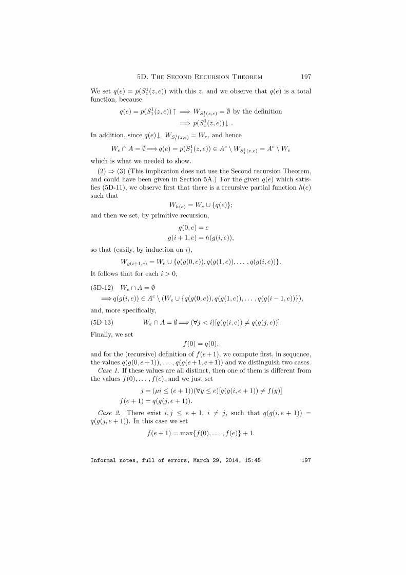
5D. The Second Recursion Theorem 197
We set q(e) = p(S11(z, e)) with this z, and we observe that q(e) is a total
function, because
q(e) = p(S11(z, e)) ↑ =⇒ WS1
1(z,e) = ∅ by the definition
=⇒ p(S11(z, e))↓ .
In addition, since q(e)↓ , WS11(z,e) = We, and hence
We ∩A = ∅=⇒ q(e) = p(S11(z, e)) ∈ Ac \WS1
1(z,e) = Ac \We
which is what we needed to show.(2) ⇒ (3) (This implication does not use the Second recursion Theorem,
and could have been given in Section 5A.) For the given q(e) which satis-fies (5D-11), we observe first that there is a recursive partial function h(e)such that
Wh(e) = We ∪ q(e);and then we set, by primitive recursion,
g(0, e) = e
g(i + 1, e) = h(g(i, e)),
so that (easily, by induction on i),
Wg(i+1,e) = We ∪ q(g(0, e)), q(g(1, e)), . . . , q(g(i, e)).It follows that for each i > 0,
(5D-12) We ∩A = ∅=⇒ q(g(i, e)) ∈ Ac \ (We ∪ q(g(0, e)), q(g(1, e)), . . . , q(g(i− 1, e))),
and, more specifically,
We ∩A = ∅=⇒ (∀j < i)[q(g(i, e)) 6= q(g(j, e))].(5D-13)
Finally, we setf(0) = q(0),
and for the (recursive) definition of f(e+1), we compute first, in sequence,the values q(g(0, e+1)), . . . , q(g(e+1, e+1)) and we distinguish two cases.
Case 1. If these values are all distinct, then one of them is different fromthe values f(0), . . . , f(e), and we just set
j = (µi ≤ (e + 1))(∀y ≤ e)[q(g(i, e + 1)) 6= f(y)]f(e + 1) = q(g(j, e + 1)).
Case 2. There exist i, j ≤ e + 1, i 6= j, such that q(g(i, e + 1)) =q(g(j, e + 1)). In this case we set
f(e + 1) = maxf(0), . . . , f(e)+ 1.
Informal notes, full of errors, March 29, 2014, 15:45 197

198 5. Introduction to computability theory
It is clear that f(e) is recursive and one-to-one, and that it is a productivefunction for Ac follows immediately from (5D-13) and (5D-12).
(3) ⇒ (4). If q(e) is a productive function for the complement Ac andB is any r.e. set, then (by the Second Recursion Theorem) there is somenumber z such that
ϕz(x, t) =
1 if x ∈ B & t = q(S1
1(z, x))↑ otherwise;
the functionf(x) = q(S1
1(z, x))
is one-to-one (as a composition of one-to-one functions), and it reduces Bto A, as follows.
If x ∈ B, then WS11(z,x) = q(S1
1(z, x) = f(x), and
f(x) /∈ A =⇒ WS11(z,x) ∩A = ∅
=⇒ q(S11(z, x)) ∈ Ac \WS1
1(z,x)
=⇒ f(x) ∈ Ac \ f(x),which is a contradiction; hence f(x) ∈ A. On the other hand, if x /∈ B,then WS1
1(z,x) = ∅ ⊆ Ac, hence f(x) = q(S11(z, x)) ∈ Ac. a
5E. The arithmetical hierarchy
The semirecursive (Σ01) relations are of the form
(∃y)Q(~x, y)
where Q(~x, y) is recursive, and so they are just one existential quantifier“away” from the recursive relations in complexity. The next definition givesus a useful tool for the classification of complex, undecidable relations.
Definition 5E.1. The classes (sets) of relations Σ0k, Π0
k, ∆0k are defined
recursively, as follows:
Σ01 : the semirecursive relations
Π0k = ¬Σ0
k : the negations (complements) of relations in Σ0k
Σ0k+1 = ∃NΠ0
k : the relations which satisfy an equivalence
P (~x) ⇐⇒ (∃y)Q(~x, y), where Q(~x, y) is Π0k
∆0k = Σ0
k ∩Π0k : the relations which are both Σ0
k and Π0k.
A set A is in one of these classes Γ if the relation x ∈ A is in Γ.
Informal notes, full of errors, March 29, 2014, 15:45 198

5E. The arithmetical hierarchy 199
5E.2. Canonical forms. These classes of the arithmetical hierarchyare (obviously) characterized by the following “canonical forms”, in thesense that a given relation P (~x) is in a class Γ if it is equivalent with thecanonical form for Γ, with some recursive Q:
Σ01 : (∃y)Q(~x, y)
Π01 : (∀y)Q(~x, y)
Σ02 : (∃y1)(∀y2)Q(~x, y1, y2)
Π02 : (∀y1)(∃y2)Q(~x, y1, y2)
Σ03 : (∃y1)(∀y2)(∃y3)Q(~x, y1, y2, y3)
...
A trivial corollary of these canonical forms is that:
Proposition 5E.3. The relations which belong to some Σ0k or some Π0
k
are precisely the arithmetical relations.
Proof. Each primitive recursive relation is arithmetical, by Theorem4B.13 and Lemma 4B.2, and then (inductively) every Σ0
k and every Π0k
relation is arithmetical, because the class of arithmetical relations is closedunder negation and quantification on N. For the other direction, we noticethat relations defined by quantifier-free formulas are (trivially) recursive,and that every arithmetical relation is defined by some formula in prenexform with quantifier-free matrix; and by introducing dummy quantifiers, ifnecessary, we may assume that the quantifiers in the prefix are alternatingand start with an ∃, so that the relation defined by each formula is in someΣ0
k. aTheorem 5E.4. (1) For each k ≥ 1, the classes Σ0
k, Π0k, and ∆0
k areclosed for (total) recursive substitutions and for the operations &, ∨, ∃≤and ∀≤. In addition:• Each ∆0
k is closed for negation ¬.• Each Σ0
k is closed for ∃N, existential quantification over N.• Each Π0
k is closed for ∀N, universal quantification over N.(2) For each k ≥ 1,
Σ0k ⊆ ∆0
k+1,(5E-14)
and hence the arithmetical classes satisfy the following diagram of inclu-sions:
Σ01 Σ0
2 Σ03
⊆ ⊆ ⊆ ⊆ ⊆ ⊆∆0
1 ∆02 ∆0
3 · · ·⊆ ⊆ ⊆ ⊆ ⊆ ⊆
Π01 Π0
2 Π03
Informal notes, full of errors, March 29, 2014, 15:45 199

200 5. Introduction to computability theory
Proof. First we verify the closure of all the arithmetical classes forrecursive substitutions, by induction on k; the proposition is known fork = 1 by 5A.7, and (inductively), for the case of Σ0
k+1, we compute:
P (~x) ⇐⇒ R(f1(~x), . . . , fn(~x))⇐⇒ (∃y)Q(f1(~x), . . . , fn(~x), y)
where Q ∈ Π0k, by definition
⇐⇒ (∃y)Q′(~x, y)where Q′ ∈ Π0
k by the induction hypothesis.
The remaining parts of (1) are easily shown (all together) by induction onk, using the transformations in the proof of 5A.7.
We show (2) by induction on k, where, in the basis, if
P (~x) ⇐⇒ (∃y)Q(~x, y)
with a recursive Q, then P is surely Σ02, since each recursive relation is Π0
1;but a semirecursive relation is also Π0
2, since, obviously,
P (~x) ⇐⇒ (∀z)(∃y)Q(~x, y)
and the relationQ1(~x, z, y) ⇐⇒ Q(~x, y)
is recursive. The induction step of the proof is practically identical, andthe inclusions in the diagram follow easily from (5E-14) and simple com-putations. a
More interesting is the next theorem which justifies the appellation “hi-erarchy” for the classes Σ0
k, Π0k:
Theorem 5E.5 (Kleene).
(1) (Enumeration for Σ0k) For each k ≥ 1 and each n ≥ 1, there is an
n+1-ary relation S0k,n(e, ~x) in the class Σ0
k which enumerates all the n-ary,Σ0
k relations, i.e., P (~x) is Σ0k if and only if for some e,
P (~x) ⇐⇒ S0k,n(e, ~x).
(2) (Enumeration for Π0k) For each k ≥ 1 and each n ≥ 1, there is an
n + 1-ary relation P 0k,n(e, ~x) in Π0
k which enumerates all the n-ary, Π0k
relations, i.e., P (~x) is Π0k if and only if, for some e,
P (~x) ⇐⇒ P 0k,n(e, ~x).
(3) (Hierarchy Theorem) The inclusions in the Diagram of Proposi-tion 5E.4 are all strict, i.e.,
Informal notes, full of errors, March 29, 2014, 15:45 200

5E. The arithmetical hierarchy 201
Σ01 Σ0
2 Σ03
( ( ( ( ( (∆0
1 ∆02 ∆0
3 · · ·( ( ( ( ( (
Π01 Π0
2 Π03
Proof. For (1) and (2) we set, recursively,
S01,n(e, ~x) ⇐⇒ (∃y)Tn(e, ~x, y)
P 0k,n(e, ~x) ⇐⇒ ¬S0
k,n(e, ~x)
S0k+1,n(e, ~x) ⇐⇒ (∃y)P 0
k,n+1(e, ~x, y),
and the proofs are easy, with induction on k. For (3), we observe that the“diagonal” relation
Dk(x) ⇐⇒ S0k,1(x, x)
is Σ0k but cannot be Π0
k, because, if it were, then for some e we would have
¬S0k,1(x, x, ) ⇐⇒ S0
k,1(e, x)
which is absurd when x = e. It follows that for each k, there exist relationswhich are Σ0
k but not Π0k, and from this follows easily the strictness of all
the inclusions in the diagram. aTheorem 5E.5 gives an alternative proof—and a better understanding—
of Tarski’s Theorem 4A.5, that the truth set of arithmetic TruthN is notarithmetical, cf. Problem x5.30.
Definition 5E.6 (Classifications). A (complete) classification of a re-lation P (~x) (in the arithmetical hierarchy) is the determination of “theleast” arithmetical class to which P (~x) belongs, i.e., the proof of a propo-sition of the form
P ∈ Σ0k \Π0
k, P ∈ Π0k \ Σ0
k, or P ∈ ∆0k+1 \ (Σ0
k ∪Π0k);
for example, in 5B.11 we showed that
e | We 6= ∅ ∈ Σ01 \Π0
1.
The complete classification of a relation P is sometimes very difficult,and we are often satisfied with the computation of some “upper bound”,i.e., some k such that P ∈ Σ0
k or P ∈ Π0k. The basic method for the
computation of a “lower bound,” when this can be done, is to show thatthe given relation is complete in some class Σ0
k or Π0k as in the next result.
Proposition 5E.7. (1) The set F = e | ϕe is total is Π02 but it is not
Σ02.(2) The set Fin = e | We is finite is Σ0
2 \Π02.
Informal notes, full of errors, March 29, 2014, 15:45 201

202 5. Introduction to computability theory
Proof. (1) The upper bound is obvious, since
e ∈ F ⇐⇒ (∀x)(∃y)T1(e, x, y).
To show (by contradiction) that F is not Σ02, suppose P (x) is any Π0
2
relation, so that
P (x) ⇐⇒ (∀u)(∃v)Q(x, u, v)
with a recursive Q(x, u, v), and set
f(x, u) = µvQ(x, u, v).
If f is a code of this (recursive) partial function f(x, u), then
P (x) ⇐⇒ (∀u)[f(x, u)↓ ]
⇐⇒ (∀u)[S11(f , x)(u)↓ ]
⇐⇒ S11(f , x) ∈ F ;
it follows that if F were Σ02, then every Π0
2 would be Σ02, which contradicts
the Hierarchy Theorem 5E.5 (3).
(2) The upper bound is again trivial,
e ∈ Fin ⇐⇒ (∃k)(∀x)[x ∈ We =⇒x ≤ k].
For the lower bound, let P (x) be any Σ02 relation, so that
P (x) ⇐⇒ (∃u)(∀v)Q(x, u, v)
with a recursive Q. We set
g(x, u) = µy(∀i ≤ u)¬Q(x, i, (y)i),
so that if g is a code of g, then
(∃u)(∀v)Q(x, u, v) ⇐⇒ u | g(x, u)↓ is finite
⇐⇒ u | g(x, u)↓ is finite
⇐⇒ u | S11(g, x)(u)↓ is finite,
i.e.,
P (x) ⇐⇒ S11(g, x) ∈ Fin;
but this implies that Fin is not Π02, because, if it were, then every Σ0
2
relation would be Π02, which it is not. a
Informal notes, full of errors, March 29, 2014, 15:45 202

5F. Relativization 203
5F. Relativization
The notions of µ-recursiveness in 4E.5 and reckonability in 4E.9 “rela-tivize” naturally to a “given” partial function as follows.
Definition 5F.1. For a fixed partial function p : Nm N:(1) A µ-recursive derivation from (or relative to) p is a sequence
of partial functions on Nf1, f2, . . . , fk,
where each fi is S, or a constant Cnq or a projection Pn
i , or p, or is definedby composition, primitive recursion or minimalization from functions beforeit in the sequence; and a partial function f : Nn N is µ-recursive in pif it occurs in a µ-recursive derivation from p.
(2) For each partial function p, let Qp be Robinson’s system in theextension of the language of arithmetic with a single m-ary function symbolp and with the additional axioms
Dp = p(∆x1, . . . , ∆xm) = ∆w | p(x1, . . . , xm) = w,which express formally the graph of p. A partial function f is reckonablein p, if there is a formula F(v1, . . . , vn, y, p) of Qp, such that for all ~x,w,
f(~x) = w ⇐⇒ Qp ` F(∆x1, . . . , ∆xn, ∆w, p).
These notions express two different ways in which we can compute afunction f given access to the values of p, and they behave best when the“given” p is total, in which case they coincide:
Proposition 5F.2. If p : Nm → N is a total function, then, for every(possibly partial) f ,
f is µ-recursive in p ⇐⇒ f is reckonable in p.
Proof is a simple modification of the proof of 4E.10. aWe will just say
f is recursive in p or f is Turing-recursive in p
for this notion of reduction of a partial function to a total one, the referenceto “Turing” coming from a third equivalent definition which involves “Tur-ing machines with oracles”. The notion is cleanest and easiest to study onsets, via their characteristic functions.
5F.3. Turing reducibility and Turing degrees. For any two setsA,B ⊆ N, we set
A ≤T B ⇐⇒ A is recursive in (or Turing reducible to) B
⇐⇒ χA is recursive in χB ,
Informal notes, full of errors, March 29, 2014, 15:45 203

204 5. Introduction to computability theory
where χA, χB are the (total) characteristic functions of A and B. We alsoset
A ≡T B ⇐⇒ A ≤T B & B ≤T A,
and we assign to each set A its degree (of unsolvability)
deg(A) = B | B ≡T A.Proposition 5F.4. (1) A ≤m B =⇒A ≤T B, but the converse is not
always true.(2) If A ≤T B and B ≤T C, then A ≤T C.(3) If B is recursive, then, for every A,
A ≤T B ⇐⇒ A is recursive,
and sodeg(∅) = deg(N) = A | A is recursive.
Less trivial are the following three properties, with which the seriousstudy of degrees of unsolvability starts:
(1) There is no maximal Turing degree, i.e., for each A, there is someB such that A <T B. (For example, if A is recursive, then A <T K, sinceA ≤1 K, but we can’t have K ≤T A since this would imply that K isrecursive.)
(2) (The Kleene-Post Theorem). There exist Turing-incomparablesets A and B, i.e.,
A 6≤T B and B 6≤T A.(5F-15)
(3) (The Friedberg-Mucnik Theorem, strengthening (2) and resolv-ing Post’s Problem). There exist Turing-incomparable, r.e. sets A, andB.
We will not pursue here the theory of degrees of unsolvability, which is aseparate (intricate and difficult) research area in the mathematical theoryof computability. We turn instead to another use of the relativizationprocess, which yields natural notions of computability for operations whichtake partial function arguments.
Definition 5F.5 (Functionals). A (partial) functional is any partial func-tion α(x1, . . . , xn, p1, . . . , pm) of n number arguments and m partial func-tion arguments, such that for i = 1, . . . ,m, pi ranges over the ki-ary partialfunctions on N and (when it takes a value), α(x1, . . . , xn, p1, . . . , pm) ∈ N.We view every partial function f(~x) as a functional 0 partial function ar-guments. More interesting examples include:
α1(x, p) = p(x + 1)
α2(x, p, q) = if x = 0 then p(x) else q(x, p(x− 1))
Informal notes, full of errors, March 29, 2014, 15:45 204

5F. Relativization 205
α3(p) =
1 if p(0)↓ or p(1)↓↑ otherwise
α4(p) =
1 if p(0)↓0 otherwise
α5(p) =
1 if (∀x)[p(x)↓ ]↑ otherwise
From these examples, we might say that α1 and α2 are “recursive”, in thesense that we can see a direct method for computing their values if we haveaccess to a “oracles” who can respond to questions of the form
What is p(x)? What is q(x, y)?
for specific x. To compute α2(x, p), for example, if x = 0 we request ofthe oracle the value p(0, x) and give it as output, while, if x > 0, then wefirst request the value v = p(x − 1, 0), and then we request and give asoutput the value p(x, v). On the other hand, there is no obvious way tocompute the values of α4 and α5 in this way, unless we can ask the oraclequestions about the domain of convergence of p, a conception which doesnot yield a natural and useful notion of computability. Finally, α3(p) isa borderline case, which appears to be recursive if we can ask the oracle“non-deterministic” questions of the form
what is p(0) or p(1)?,
which looks iffy—or, at the least, suggests a different notion of “non-deterministic computability” for functionals.
Definition 5F.6 (Recursive functionals). We make these two notions offunctional computability precise, using the relativization process.
(1) A µ-recursive (functional) derivation (in one, m-ary partialfunction variable) is a sequence of functionals
α1(~x1, p), . . . , αm(~xm, p)
in which each αi is S, Cnq or Pn
j (not depending on p); an evaluationfunctional
evm(x1, . . . , xm, p) = p(x1, . . . , xm)(5F-16)
which introduces dependence on p; or it is defined from previously listedfunctionals by composition, primitive recursion or minimalization, whichare defined as before, e.g,
αi(~x, p) = µy[αj(~x, y, p) = 0] (j < i).
A functional is µ-recursive, or just recursive, if it occurs in some µ-recursive derivation.
Informal notes, full of errors, March 29, 2014, 15:45 205

206 5. Introduction to computability theory
(2) A functional α(~x, p) is reckonable (or non-deterministically re-cursive) if there is a formula F(v1, . . . , vn, y, p) in the system Qp introducedin (2) of 5F.1, such that for all ~x,w and p,
α(~x, p) = w ⇐⇒ Qp ` F(∆x1, . . . , ∆xn, ∆w, p).(5F-17)
5F.7. Remark. There is no formula F(v1, . . . , vn, y, p) such that, forall ~x, w and p
p(~x) = w ⇐⇒ F(∆x1, . . . , ∆xn, ∆w)(A)
Qp ` (∃!y)F(∆x1, . . . , ∆xn, y),(B)
simply because if (A) holds for all p, then the formula on the right of (B) isnot true, whenever p is not a totally defined function. This means that thesimplest evaluation functional (5F-16) is not “numeralwise representable”in Q, in the most natural extension of this notion to functionals, which iswhy we have not introduced it.
Proposition 5F.8. Every recursive functional is reckonable.
Proof is a minor modification of the argument for (1) =⇒ (2) of The-orem 4E.10 (skipping the argument for the characteristic property of nu-meralwise representability which does not hold here), and we will skip it.a
To separate recursiveness from reckonability for functionals, we need tointroduce some basic notions, all of them depending on the following, par-tial ordering of partial functions of the same arity.
Definition 5F.9. For any two, m-ary partial functions p and q, we set
p ≤ q ⇐⇒ (∀~x,w)[p(~x) = w =⇒ q(~x) = w],
i.e., if the domain of convergence of p is a subset of the domain of con-vergence of q, and q agrees with p whenever they are both defined. Forexample, if ∅ is the nowhere-defined m-ary partial function, then, for everym-ary q, ∅ ≤ q; and, at the other extreme,
(∀~x)p(~x)↓ & p ≤ q =⇒ p = q.
Proposition 5F.10. For each m, ≤ is a partial ordering of the set ofall m-ary partial functions, i.e.,
p ≤ p, [p ≤ q & q ≤ r] =⇒ p ≤ r, [p ≤ q & q ≤ p] =⇒ p = q.
Proof is simple and we will skip it. aDefinition 5F.11. A functional α(~x, p) is:1. monotonic (or monotone), if for all partial functions p, q, and all ~x,
w,[α(~x, p) = w & p ≤ q] =⇒α(~x, q) = w;
Informal notes, full of errors, March 29, 2014, 15:45 206

5F. Relativization 207
2. continuous, if for each p and all ~x, w,
α(~x, p) = w =⇒ (∃r)[r ≤ p & α(~x, r) = w & r is finite],
where a partial function is finite if its domain of convergence is finite;and
3. deterministic, if for each p and all ~x, w,
α(~x, p) = w =⇒ (∃!r ≤ p)[α(~x, r) = w & (∀r′ ≤ r)[α(~x, r′)↓ =⇒ r′ = r]].
5F.12. Exercise. Give counterexamples to show that no two of theseproperties imply the third.
Theorem 5F.13. (1) Every reckonable functional is monotonic and con-tinuous.
(2) Every recursive functional is monotonic, continuous and determinis-tic.
(3) There are reckonable functionals which are not deterministic.
Proof. (1) is immediate, using the (corresponding) properties of proofs:for example, if
Qp ` F(∆x1, . . . , ∆xn, ∆w, p)
for some p, ~x and w, then the proof can only use a finite number of theaxioms in Qp, which “fix” p only on a finite set of arguments—and if r isthe (finite) restriction of p to this set, then
Qr ` F(∆x1, . . . , ∆xn, ∆w, r),
so that α(~x, r) = w.(2) is proved by induction on a given µ-recursive derivation. There are
several cases to consider, but the arguments are simple and we will skipthem.
(3) The standard example is
α3(p) =
1 if p(0)↓ or p(1)↓↑ otherwise
as above, which is not deterministic because if p(0) = p(1) = 0 and p(x) ↑for all x > 1, then there is no least r ≤ p which determines the valueα3(p) = 1. a
Part (1) of this theorem yields a simple normal form for reckonable func-tionals which characterizes them without reference to any formal systems.We need another coding.
Informal notes, full of errors, March 29, 2014, 15:45 207

208 5. Introduction to computability theory
5F.14. Coding of finite partial functions and sets. For each a ∈ Nand each m ≥ 1,
d(a, x) =
(a)x−· 1 if x < lh(a) & (a)x > 0,
↑ otherwise
da(x) = d(a, x),Dx = i | dx(i)↓
dma (~x) = dm(a, ~x) = d(a, 〈~x〉) (~x = x1, . . . , xm).
Note that, easily, each partial function dm(a, ~x) is recursive; the sequence
dm0 , dm
1 , . . .
enumerates all finite partial functions of m arguments; and the sequence
D0, D1, . . .
enumerates all finite sets, so that the binary relation of membership
i ∈ Dx ⇐⇒ i < lh(x) & (x)i > 0,
is primitive recursive.
Theorem 5F.15 (Normal form for reckonable functionals). A functionalα(~x, p) is reckonable if and only if there exists a semirecursive relationR(~x,w, a), such that for all ~x, w and p,
α(~x, p) = w ⇐⇒ (∃a)[dma ≤ p & R(~x,w, a)].(5F-1)
Proof. Suppose first that α(~x, p) is reckonable, and compute:
α(~x, p) = w ⇐⇒ (∃ finite r ≤ p)[α(~x, r) = w] (by 5F.13)
⇐⇒ (∃a)[dma ≤ p & α(~x, dm
a ) = w)].
Thus, it is enough to prove that the relation
R(~x,w, a) ⇐⇒ α(~x, dma ) = w
is semirecursive; but if (5F-17) holds with some formula F(v1, . . . , vm, y, p),then
R(~x,w, a) ⇐⇒ Qdma` F(∆x1, . . . , ∆xn, ∆w, p)
⇐⇒ Q ` σm,a,p → F(∆x1, . . . , ∆xn, ∆w, p)
where σm,a,p is the finite conjunction of equations
p(∆u1, . . . , ∆um) = ∆dma (u1, . . . , um),
one for each u1, . . . , um in the domain of dma . A code of the sentence on the
right can be computed primitive recursively from ~x,w, a, so that R(~x,w, a)is reducible to the relation of provability in Q and hence semirecursive.
Informal notes, full of errors, March 29, 2014, 15:45 208

5G. Effective operations 209
For the converse, we observe that with the same σm,a,p we just used andfor any m-ary p,
dma ≤ p ⇐⇒ Qp ` σm,a,p,
and that, with some care, this σm,a,p can be converted to a formula σ∗(a, p)with the free variable a, in which bounded quantification replaces the blunt,finite conjunction so that
dma ≤ p ⇐⇒ Qp ` σ∗(∆a, p).(5F-2)
Assume now that α(~x, p) satisfies (5F-1), choose a primitive recursive rela-tion P (~x,w, a, z) such that
R(~x,w, a) ⇐⇒ (∃z)P (~x,w, a, z),
choose a formula P(v1, . . . , vn, vn+1, vn+2, z) which numeralwise expressesP in Q, and set
F(v1, . . . , vn, vn+1, vn+2)) ≡ (∃a)[σ∗(a, p) & (∃z)P(v1, . . . , vn, vn+1, a, z)]].
Now,
Qp ` F(∆x1, . . . , ∆xn,∆w, p)
⇐⇒ Qp ` (∃a)[σ∗(a, p)
& (∃z)[P(∆x1, . . . , ∆xn, ∆w, a, z)]]
⇐⇒ α(~x, p) = w,
with the last equivalence easy to verify, using the soundness of Qp. aThere is no simple normal form of this type for recursive functionals,
because predicate logic is not well suited to expressing “determinism”.
5G. Effective operations
Intuitively, a functional α(~x, p) is recursive in either of the two ways thatwe made precise, if its values can be computed effectively and uniformlyfor all partial functions p, given access only to specific values of p—whichsimply means that the evaluation functional (5F-16) is declared recursive.In many cases, however, we are interested in the values α(~x, p) only forrecursive partial functions p, and then we might make available to thecomputation procedure some code of p, from which (perhaps) more thanthe values of p can be extracted.
Definition 5G.1. The associate of a functional α(~x, p) is the partialfunction
fα(~x, e) = α(~x, ϕe),(5G-3)
and we call α(~x, p) an effective operation if its associate is recursive.
Informal notes, full of errors, March 29, 2014, 15:45 209

210 5. Introduction to computability theory
Note that this imposes no restriction on the values α(~x, p) for non-recursive p, and so, properly speaking, we should think of effective opera-tions as (partial) functions on recursive partial functions, not on all partialfunctions—this is why the term “operation” is used. For purposes of com-parison with recursive functionals, however, it is convenient to considereffective operations as functionals, with arbitrary values on non-recursivearguments, as we did in the precise definition.
Proposition 5G.2. A recursive partial function f(~x, e) is the associateof some effective operation if and only if it satisfies the invariance condition
ϕe = ϕm =⇒ f(~x, e) = f(~x,m);(5G-4)
and if f satisfies this condition, then it is the associate of the effectiveoperation
α(~x, ϕe) = f(~x, e),
(with α(~x, p) defined arbitrarily when p is not recursive).
Proof is immediate. a
Theorem 5G.3. Every reckonable functional (and hence every recur-sive functional) is an effective operation.
Proof. This is immediate from the Normal Form Theorem for reckon-able functionals 5F.15; because if f(~x, e) is the associate of α(~x, p), then
f(~x, e) = w ⇐⇒ (∃a)[dma ≤ ϕe & R(~x,w, a)]
with a semirecursive R(~x,w, a) by 5F.15, and so the graph of f is semire-cursive and f is recursive. a
Definition 5G.4. A functional α(~x, p) is operative if ~x = x1, . . . , xn
varies over n-tuples and p over n-ary partial functions, for the same n, sothat the fixed point equation
p(~x) = α(~x, p)(5G-5)
makes sense. Solutions of this equation are called fixed points of α.
Theorem 5G.5 (The Fixed Point Lemma). Every operative effective op-eration α has a recursive fixed point, i.e., there exists a recursive partialfunction p such that, for all ~x,
p(~x) = α(~x, p).
Proof. The partial function
f(z, ~x) = α(~x, ϕz)
Informal notes, full of errors, March 29, 2014, 15:45 210

5G. Effective operations 211
is recursive, and so, by the Second Recursion Theorem, there is some z∗
such that
ϕz∗(~x) = f(z∗, ~x)= α(~x, ϕz∗);
and so p = ϕz∗ is a fixed point of α. a5G.6. Remark. By an elaboration of these methods (or different ar-
guments), it can be shown that every effective operation has a recursiveleast fixed point : i.e., that for some recursive partial function p, the fixedpoint equation (5G-5) holds, and in addition, for all q,
(∀~x)[q(~x) = α(~x, q)]=⇒ p ≤ q.
The Fixed Point Lemma applies to all reckonable operative functionals,and it is a powerful tool for showing easily the recursiveness of partial func-tions defined by very general recursive definitions, for example by doublerecursion:
5G.7. Example. If g1, g2, g3, π1, π2 are total recursive functions andf(x, y, z) is defined by the double recursion
f(0, y, z) = g1(y, z)f(x + 1, 0, z) = g2(f(x, π1(x, y, z), z), x, y, z)
f(x + 1, y + 1) = g3(f(x + 1, y, π2(x, y, z)), x, y, z),
then f(x, y, z) is recursive.
Proof. The functional
h(x, y, z, p) =
g1(y, z) if x = 0g2(p(x−· 1, π1(x−· 1, 0, z), z), x−· 1, 0, z) otherwise, if y = 0g3(p(x, y−· 1, Π0
2(x, y−· 1, z)), x, y−· 1, z) otherwise
is recursive, and so it has a recursive fixed point f(x, y, z), which, eas-ily, satisfies the required equations. It remains to show that f(x, y, z) isa total function, and we do this by showing by an induction on x that(∀x)f(x, y, z) ↓ ; both the basis case and the induction step require sepa-rate inductions on y. a
The converse of Theorem 5G.3 depends on the following, basic result.
Lemma 5G.8. Every effective operation is monotonic and continuouson recursive partial arguments.
Proof. To simplify the argument we consider only effective operationsof the form α(p), with no numerical argument and a unary partial functionargument, but the proof for the general case is only notationally morecomplex.
Informal notes, full of errors, March 29, 2014, 15:45 211

212 5. Introduction to computability theory
To show monotonicity, suppose p ≤ q, where
p = ϕe and q = ϕm,
and let f be a code of the associate of α, so that for every z,
α(ϕz) = f(z).
Suppose also thatα(ϕe) = w;
we must show that α(ϕm) = w.The relation
R(z, x, v) ⇐⇒ ϕe(x) = v or [f(z)↓ & ϕm(x) = v]
is semirecursive; the hypothesis ϕe ≤ ϕm implies that
R(z, x, v) =⇒ϕm(x) = v;
hence R(z, x, v) is the graph of some recursive partial function g(z, x); andso, by the Second recursion Theorem, there is some number z∗ such thatϕz∗(x) = g(z∗, x), so that
ϕz∗(x) = v ⇐⇒ ϕe(x) = v or [f(z∗)↓ & ϕm(x) = v].(5G-6)
We now observe that:(1a) α(ϕz∗) = f(z∗) = w; because, if not, then ϕz∗ = ϕe from (5G-6),
and so α(ϕz∗) = α(ϕe) = w.(1b) ϕz∗ = ϕm, directly from the hypothesis ϕe ≤ ϕm and (1a).It follows that α(ϕm) = α(ϕz∗) = w.The construction for the proof of continuity is a small variation, as fol-
lows. First, we find using the Second recursion Theorem some z∗ suchthat
ϕz∗(x) = v ⇐⇒ (∀u ≤ x)¬[T1(f , z∗, u) & U(u) = w] & ϕe(x) = v,
(5G-7)
and we observe:(2a) α(ϕz∗) = w. Because, if not, then
(∀u)¬[T1(f , z∗, u) & U(u) = w],
and hence, for every x,
(∀u ≤ x)¬[T1(f , z∗, u) & U(u) = w],
and so, from (5G-7), ϕz∗ = ϕe and α(ϕz∗) = α(ϕe) = w.(2b) ϕz∗ ≤ ϕe, directly from (5G-7).(2c) The partial function ϕz∗ is finite, because it converges only when
x < (µu)[T1(f , z∗, u) & U(u) = w].(5G-8) a
Informal notes, full of errors, March 29, 2014, 15:45 212

5G. Effective operations 213
Theorem 5G.9 (Myhill-Shepherdson). For each effective operation α(~x, p),there is a reckonable functional α∗(~x, p) such that for all recursive partialfunctions p,
α(~x, p) = α∗(~x, p).(5G-9)
Proof. By the Lemma,
α(~x, ϕe) = w ⇐⇒ (∃a)[dma ≤ ϕe & α(~x, dm
a ) = w],
and so (5G-9) holds with
α∗(~x, p) = w ⇐⇒ (∃a)[dma ≤ p & α(~x, dm
a ) = w].(5G-10)
To show that this α∗ is reckonable, note that (by an easy application ofthe Sm
n -Theorem) there is a primitive recursive u(a) such that
dma = ϕu(a),
and so the partial function
α(~x, dma ) = fα(~x, u(a))
is recursive, its graph is semirecursive, and (5G-10) with Theorem 5F.15imply that α∗ is reckonable. a
5G.10. Remark. It is natural to think of a functional α(~x, p) as in-terpreting a program A, which computes some function f(~x) but requiresfor the computations some unspecified partial function p—and hence, Amust be “given” p in addition to the arguments ~x. Now if p could be anypartial function whatsoever, then the only reasonable way by which A canbe “given” p is through its values: we imagine that A can look up a tableor ask an “oracle” for p(u), for any specific u, during the computation.We generally refer to this manner of “accessing” a partial function by aprogram as call-by-value, and it is modeled mathematically by recursive orreckonable functionals, depending on whether the program A is determin-istic or not. On the other hand, if it is known that p = ϕe is a recursivepartial function, then some code e of it may be given to A, at the start ofthe computation, so that A can compute any p(u) that it wishes, but also(perhaps) infer general properties of p from e, and use these properties inits computations; this manner of accessing a recursive partial function is(one version of) call-by-name, and it is modeled mathematically by effectiveoperations.
One might suspect that given access to a code of p, one might be ableto compute effectively partial functions (depending on p) which cannotbe computed when access to p is restricted in call-by-value fashion. TheMyhill-Shepherdson Theorem tells us that, for non-deterministic programs,this cannot happen—knowledge of a code of p does not enlarge the classof partial functions which can be non-deterministically computed from it.
Informal notes, full of errors, March 29, 2014, 15:45 213

214 5. Introduction to computability theory
Note that this is certainly false for deterministic computations, because ofthe basic example α3(p) in 5F.5, which is reckonable but not recursive.
5H. Problems for Chapter 5
Problem x5.1. Prove that if R(x1, . . . , xn) is a recursive relation, thenthere exists a formula R(v1, . . . , vn) in the language of arithmetic such that
R(x1, . . . , xn)=⇒Q ` R(∆x1 . . . , ∆xn)
and ¬R(x1, . . . , xn)=⇒Q ` ¬R(∆x1 . . . , ∆xn).
Problem x5.2. Prove that every axiomatizable, complete theory is de-cidable.
Problem x5.3. Show that the class of recursive partial functions is uni-formly closed under definition by primitive recursion in the following, pre-cise sense: there is a primitive recursive function un(e,m), such that iff(y, ~x) is defined by the primitive recursion
f(0, ~x) = ϕe(~x), f(y + 1, ~x) = ϕm(f(y, ~x), y, ~x),
then f(y, ~x) = un(e,m)(y, ~x).
Problem x5.4. Define a total, recursive, one-to-one function un(e, i),such that for all e, i, ~x,
un(e, i)(~x) = e(~x).
(In particular, each recursive partial function has, effectively, an infinitenumber of distinct codes.)
Problem x5.5. Show that the partial function
f(e, u) = 〈ϕe((u)0), ϕe((u)1), . . . , ϕe((u)lh(u)−· 1)〉
is recursive.
Problem x5.6 (Craig’s Lemma). Show that a theory T has a primitiverecursive set of axioms if and only if it has an r.e. set of axioms.
Problem x5.7∗. Prove that there is a recursive relation R(x) which isnot primitive recursive.
Problem x5.8. Suppose R(~x,w) is a semirecursive relation such thatfor each ~x there exist at least two distinct numbers w1 6= w2 such thatR(~x,w1) and R(~x,w2). Prove that there exist two, total recursive functionsg(~x) and h(~x), such that for all ~x,
R(~x, g(~x)) & R(~x, h(~x)) & g(~x) 6= h(~x).
Informal notes, full of errors, March 29, 2014, 15:45 214

5H. Problems for Chapter 5 215
Problem x5.9∗. Suppose R(~x,w) is a semirecursive relation such thatfor each ~x, there exists at least one w such that R(~x,w).
(a) Prove that there is a total recursive function f(n, ~x) such that
R(~x,w) ⇐⇒ (∃n)[w = f(n, ~x)].(∗)(b) Prove that if (in addition), for each ~x, there exist infinitely many
w such that R(~x,w), then there exists a total, recursive f(n, ~x) whichsatisfies (∗) and which is one-to-one, i.e.,
m 6= n =⇒ f(m,~x) 6= f(n, ~x).
Problem x5.10. Prove that a relation P (~x) is Σ01 if and only if it is
definable by a Σ1 formula, in the sense of Definition 4C.11.
Problem x5.11. Show that there is a recursive, partial function f(e)such that
We 6= ∅=⇒ [f(e)↓ & f(e) ∈ We].
Problem x5.12. Prove or give a counterexample to each of the follow-ing propositions:
(a) There is a total recursive function u1(e,m) such that for all e,m,
Wu1(e,m) = We ∪Wm.
(b) There is a total recursive function u2(e, m) such that for all e,m,
Wu2(e,m) = We ∩Wm.
(c) There is a total recursive function u3(e,m) such that for all e,m,
Wu3(e,m) = We \Wm.
Problem x5.13. Prove or give a counterexample to each of the follow-ing propositions, where f : N→ N is a total recursive function and
f [A] = f(x) | x ∈ A, f−1[A] = x | f(x) ∈ A.(a) If A is recursive, then f [A] is also recursive.(b) If A is r.e., then f [A] is also r.e.(c) If A is recursive, then f−1[A] is also recursive.(d) If A is r.e., then f−1[A] is also r.e.
Problem x5.14. Prove that there is a total recursive function u(e,m)such that
Wu(e,m) = x + y | x ∈ We & y ∈ Wm.Problem x5.15. Prove that every infinite r.e. set A has an infinite re-
cursive subset.
Informal notes, full of errors, March 29, 2014, 15:45 215

216 5. Introduction to computability theory
Problem x5.16. (The Reduction Property of r.e. sets.) Prove that forevery two r.e. sets A,B, there exist r.e. sets A∗, B∗ with the followingproperties:
A∗ ⊆ A, B∗ ⊆ B, A ∪B = A∗ ∪B∗, A∗ ∩B∗ = ∅.Problem x5.17. (The Separation Property for r.,e. complements.) Prove
that if A and B are disjoint sets whose complements are r.e., then thereexists a recursive set C such that
A ⊆ C, C ∩B = ∅.Problem x5.18. (Recursively inseparable r.e. sets.) Prove that there
exist two disjoint r.e. sets A and B such that there is no recursive set Csatisfying
A ⊆ C, C ∩B = ∅.Problem x5.19. Prove that for every two r.e. sets A,B, there is a for-
mula φ(x) so that whenever x ∈ (A ∪B),
Q ` φ(x) =⇒ x ∈ A,(5H-1)Q ` ¬φ(x) =⇒ x ∈ B,(5H-2)
Q ` φ(x) or Q ` ¬φ(x)(5H-3)
Problem x5.20. Show that if A is simple and B is infinite r.e., thenthe intersection A ∩B is infinite.
Problem x5.21∗. Show that the intersection of two simple sets is sim-ple.
Problem x5.22. Prove or give a counterexample:(a) For each infinite r.e. set A, there is a total, recursive function f(x)
such that for each x,
f(x) > x & f(x) ∈ A.
(b) For each r.e. set A with infinite complement, there is a total, recursivefunction f(x) such that for each x,
f(x) > x & f(x) /∈ A.
Problem x5.23∗. Prove that if Q is interpretable in a consistent, ax-iomatizable theory T , then the set
#T = #θ | θ is a sentence and T ` θof (codes of) theorems of T is creative.
Infer that if T1 and T2 are consistent, axiomatizable theories in which Qcan be interpreted, then #T1 ≡ #T2.
Informal notes, full of errors, March 29, 2014, 15:45 216

5H. Problems for Chapter 5 217
This result is especially impressive (and a little counterintuitive) if weapply it to Q and ZFC.
Problem x5.24. Prove that there is some number z such that
Wz = z, z + 1, . . . = x | x ≥ z.Problem x5.25. Prove that for some number t and all x, ϕt(x) = t+x.
Problem x5.26. Prove that for each total, recursive function f(x) oneof the following holds:
(a) There is a number z such that f(z) is odd and for all x,
ϕz(x) = f(z + x);
or(b) there is a number w such that f(w) is even and for all x,
ϕw(x) = f(2w + x + 1).
Problem x5.27. Prove or give a counterexample: for each total, recur-sive function f(x), there is some z such that
Wf(z) = Wz.
Problem x5.28. Prove or give a counterexample: for every total, re-cursive function f(x), there is a number z such that for all t,
ϕf(z)(t) = ϕz(t).
Problem x5.29. (a) Prove that for every total, recursive function f(x),there is a number z such that
Wz = f(z).(b) Prove that there is some number z such that
ϕz(z)↓ and Wz = ϕz(z).Problem x5.30. Prove that for every arithmetical relation P (~x), there
is a 1-1, total recursive function f : Nn → N such that
P (~x) ⇐⇒ f(~x) ∈ TruthN;
infer Tarski’s Theorem 4A.5, that TruthN is not arithmetical.
Problem x5.31. Classify in the arithmetical hierarchy the set
A = e | We ⊆ 0, 1.Problem x5.32. Classify in the arithmetical hierarchy the set
A = e | We is finite and non-empty.
Informal notes, full of errors, March 29, 2014, 15:45 217

218 5. Introduction to computability theory
Problem x5.33. Classify in the arithmetical hierarchy the set
B = x | there are infinitely many twin primes p ≥ x,where p is a twin prime if both p and p + 2 are prime numbers.
Problem x5.34. Classify in the arithmetical hierarchy the relation
Q(e,m) ⇐⇒ ϕevϕm
⇐⇒ (∀x)(∀w)[ϕe(x) = w =⇒ϕm(x) = w].
Problem x5.35. Classify in the arithmetical hierarchy the set
A = e | We has at least e members.Problem x5.36. Classify in the arithmetical hierarchy the set
B = e | for some w and all x, if ϕe(x)↓ , then ϕe(x) ≤ w.(This is the set of codes of bounded recursive partial functions.)
Problem x5.37. For a fixed, unary, total recursive function f , classifyin the arithmetical hierarchy the set of all the codes of f ,
Cf = e | ϕe = f.Problem x5.38. Let A be some recursive set with non-empty comple-
ments, i.e., A ( N. Classify in the arithmetical hierarchy the set
B = e | We ⊆ A.Problem x5.39. Show that the graph
Gf (~x,w) ⇐⇒ f(~x) = w
of a total function is Σ0k if and only if it is ∆0
k.Is this also true of partial functions?
Problem x5.40. A total function f : Nn → N is limiting recursive ifthere is a total, recursive function g : Nn+1 → N such that for all ~x,
f(~x) = limm→∞
g(m,~x).
Prove that a total f(~x) is limiting recursive if and only if the graph Gf off(~x) is ∆0
2.
Problem x5.41. Prove that if T is an axiomatizable theory, then forany sentence θ,
PA ` ProvableT∪¬θ(pθq) → ProvableT (pθq).
Problem x5.42∗. Prove that if θ(v) is a full extended formula and
PA ` (∀x)ProvablePA(pθ(∆x)q) → (∀v)θ(v),
then PA ` (∀v)θ(v).
Informal notes, full of errors, March 29, 2014, 15:45 218

5H. Problems for Chapter 5 219
Problem x5.43. A function f is provably recursive in PA if there isa number e such that
f(~x) = U(µyT (e, ~x, y)) and PA ` (∀~x)(∃y)T(∆e, ~x, y),
where T(e, ~x, y) is a formula which numeralwise expresses the Kleene Tpredicate. Prove that there is a total recursive function which is not prov-ably recursive in PA.
Problem x5.44. Classify the following sets in the arithmetical hierar-chy:(a) A = e | We is a singleton.(b) B = e | We is infinite.(c) C = e | (∀x)(∃!y)〈x, y〉 ∈ We.
Informal notes, full of errors, March 29, 2014, 15:45 219


CHAPTER 6
INTRODUCTION TO FORMAL SET THEORY
We summarize here briefly the basic facts about sets which can be provedin the standard axiomatic set theories, primarily to prepare the groundfor the introduction to the metamathematics of these theories in the nextchapter.
6A. The intended universe of sets
It may be useful to review at this point our intuitive conception of thestandard model for set theory, the universe V of sets. This does not containall “arbitrary collections of objects” in Cantor’s eloquent phrase: it is wellknown that this naive approach leads to contradictions. Instead, we admitas “sets” only those collections which occur in the complete (transfinite)cumulative sequence of types—the hierarchy obtained by starting with theempty set and iterating “indefinitely” the “power operation.”
To be just a little more precise—and using “intuitive set theory”, as wehave been doing all along—suppose we are given an operation P on setswhich assigns to each set x a collection P (x) of subsets of x
y ∈ P (x) =⇒ y ⊆ x.(6A-1)
Suppose we are also given a collection S of stages, wellordered by a relation≤S , i.e., for ζ, η, ξ in S,
(6A-2) ζ ≤S ζ, (ζ ≤S η & η ≤S ξ) =⇒ ζ ≤S ξ,
(ζ ≤S η & η ≤S ζ) =⇒ ζ = η, ζ ≤S η or η ≤S ζ
(6A-3) if A ⊆ S is any collection of stages, A 6= ∅, thenthere is some ξ ∈ A such that for every η ∈ A, ξ ≤S η.
Call the least stage 0 and for ξ ∈ S, let ξ + 1 be the next stage—the leaststage which is greater than ξ. If λ is a stage 6= 0 and 6= ξ + 1 for every ξ,we call it a limit stage.
221

222 6. Introduction to formal set theory
For fixed P , S, ≤S satisfying (6A-1) – (6A-3) we define the hierarchy
Vξ = Vξ(P,S,≤S) (ξ ∈ S)
by recursion on ξ ∈ S:
V0 = ∅Vξ+1 = Vξ ∪ P (Vξ),
Vλ =⋃
ξ<λ Vξ if λ is a limit stage.
The collection of sets
V = V (P,S,≤S) =⋃
ξ∈S Vξ
is the universe generated with P as the power operation, on the stages S.It is very easy to check that
ξ ≤S η =⇒ Vξ ⊆ Vη
and that each Vξ is a transitive set, i.e.,
(x ∈ Vξ & y ∈ x) =⇒ y ∈ Vξ.
For example, suppose we take
P (x) = P(x) = y : y ⊆ xand
S = ω2 = 0, 1, 2, . . . , ω, ω + 1, ω + 2, . . . ,where the stages 0, 1, 2, . . . , ω, ω +1, ω +2, . . . are all assumed distinct andordered as we have enumerated them. In this case we obtain the universe
V Z = V (P, ω2,≤ω2) = V0 ∪ V1 ∪ V2 ∪ · · · ∪ Vω ∪ Vω+1 ∪ · · · ,
often called the universe of Zermelo. It is well known that all the familiarstructures of classical mathematics have isomorphic copies within V Z—wecan locate in V Z (faithful representations of) the natural and real numbers,all functions on the reals to the reals, etc.
For a very different universe of sets, we might choose a small poweroperation, e.g.,
Def(x) = y ⊆ x : y is elementary in the structure (x,∈¹x, tt∈x).We may want to take S quite long this time, say
S = ωω = 0, 1, 2, , . . . , ω, ω + 1, . . . , ω2, ω2 + 1, . . . , ωn, ωn + 1, . . . , . . . ,so that ωω is the union of infinitely many disjoint copies of N put side-by-side. Using notation we will justify later, set
Lωω = V (Def , ωω,≤ωω ).
It is easy to see that V Z 6⊆ Lωω , because V Z is uncountable while Lωω isa countable set. It is a little more difficult to show also that Lωω 6⊆ V Z ,so that these two constructions yield two incomparable set universes, in
Informal notes, full of errors, March 29, 2014, 15:45 222

6A. The intended universe of sets 223
which we can interpret the axioms of axiomatic set theory and check outwhich are true for each of them.
It is clear that the universe V (P,S,≤S) does not depend on the particularobjects that we have chosen to call stages but only on the length (the ordertype) of the ordering ≤S ; i.e., if the structures (S,≤S) and (S ′,≤′S) areisomorphic, then
V (P,S,≤S) = V (P,S ′,≤′S).
This definition of the universes V (P,S,≤S) is admittedly vague, and theresults about them that we have claimed are grounded on intuitive ideasabout sets and wellorderings which we have not justified. It is clear thatwe cannot expect to give a precise, mathematical definition of the basicnotions of set theory, unless we use notions of some richer theory which inturn would require interpretation. At this point, we claim only that theintuitive description of V (P,S,≤S) is sufficiently clear so we can formu-late meaningful propositions about these set universes and argue rationallyabout their truth or falsity.
Most mathematicians accept that there is a largest meaningful operationP satisfying (6A-1) above, the true power operation which takes x to thecollection P(x) of all subsets of x. This is one of the cardinal assumptionsof realistic (meaningful, not formal) set theory. Similarly, it is not unrea-sonable to assume that there is a longest collection of stages ON alongwhich we can meaningfully iterate the power operation.
Our intended standard universe of sets is then
V = V (P, ON,≤ON),
where (ON,≤ON) is the longest meaningful collection of stages—the well-ordered class of ordinal numbers, as we will call it later. The axioms ofthe standard axiomatic set theory ZFC (Zermelo-Fraenkel set theory withChoice and Foundation) are justified by appealing to this intuitive under-standing of what sets are. We will formulate it (again) carefully in thefollowing sections and then derive its most basic consequences.
What is less obvious is that if we take (ON,≤ON) to be the same “largest,meaningful collection of stages”, then the set universe
L = (Def ,ON,≤ON)
is another plausible understanding of the notion of set, Godel’s universeof constructible sets: the central theorem of this and the next Chapter isthat L also satisfies all the axioms of ZFC. Moreover, Godel’s proof of thissurprising result does not depend on the Axiom of Choice, and so it alsoshows the consistency of ZFC relative to its choiceless fragment.
Informal notes, full of errors, March 29, 2014, 15:45 223

224 6. Introduction to formal set theory
6B. ZFC and its subsystems
To simplify the formulation of the formal axioms of set theory, we statehere a simple result of logic which could have been included in Chapter 1,right after Definition 1H.11:
Proposition 6B.1 (Eliminability of descriptions). Fix a signature τ , andsuppose φ(~v, w) ≡ φ(v1, . . . , vn, w) is a full extended τ -formula and F isan n-ary function symbol not in τ .
(1) With each full, extended (τ, F )-formula θ′(~u) we can associate a full,extended τ -formula θ(~u) such that
(∀~v)(∃!w)φ(~v, w) & (∀~v)φ(~v, F (~v)) ` θ′(~u) ↔ θ(~u).
(2) Suppose T is a τ -theory axiomatized by schemes such that
T ` (∀~v)(∃!w)φ(~v, w),
and let T ′ be the (τ, F )-theory whose axioms are those of T , the sentence(∀~v)φ(~v, F (~v)), and all instances with (τ, F ) formulas of the axiom schemesof T . Then T ′ is a conservative extension of T , i.e., for all τ -sentences θ,
T ′ ` θ ⇐⇒ T ` θ.
There is also an analogous result where we add to the language a newn-ary relation symbol C and the axiom
(∀~v)[R(~v) ↔ φ(~v)] (φ(~v) full extended),(6B-4)
but it is simpler, and it can be avoided by treating (6B-4) as an abbrevia-tion. In applying these constructions we will refer to T ′ as an extension ofT by definitions.
We leave the precise definition of “axiomatization by schemes” and theproof for Problem x6.1∗. The thing to notice here is that all the set theorieswe will consider are axiomatized by schemes, and so the proposition allowsus to introduce—and use with no restriction—names for constants andoperations defined in them. If, for example,
T ` (∃!z)(∀t)[t /∈ z],
as all the theories we are considering do, we can then extend T with aconstant ∅ and the axiom
(∀t)[t /∈ ∅]and we can use this constant in producing instances of the axiom schemesof T without adding any new theorems which do not involve ∅.
We now restate for easy reference (from Definitions 1A.5, 1G.12) theaxioms of set theory and their formal versions in the language FOL(∈).
Informal notes, full of errors, March 29, 2014, 15:45 224

6B. ZFC and its subsystems 225
We will be using the common abbreviations for restricted quantification
(∃x ∈ z)φ :≡ (∃x)[x ∈ z &φ],
(∀x ∈ z)φ :≡ (∀x)[x ∈ z → φ],
(∃!x ∈ z)φ :≡ (∃y ∈ z)(∀x ∈ z)[φ ↔ y = x]
(1) Extensionality Axiom: two sets are equal exactly when they have thesame members:
(∀x, y)[x = y ↔ [(∀u ∈ x)(u ∈ y) & (∀u ∈ y)(u ∈ x)]].
(2) Emptyset and Pairing Axioms: there exists a set with no members,and for any two sets x, y, there is a set z whose members are exactlyx and y:
(∃z)(∀u)[u /∈ z], (∀x, y)(∃z)(∀u)[u ∈ z ↔ (u = x ∨ u = y)]
It follows by the Extensionality Axiom that there is exactly one emptyset and one pairing operation, and we name them ∅ and x, y, as usual.(And in the sequel we will omit this ceremony of stating separately theunique existence condition before baptizing the relevant operation with itscustomary name.)(3) Unionset Axiom: for each set x, there is exactly one set z =
⋃x
whose members are the members of members of x, i.e.,
(∀u)[u ∈ ⋃x ↔ (∃y ∈ x)[u ∈ y]].
(4) Infinity Axiom: there exists a set z such that ∅ ∈ z and z is closedunder the set successor operation x′,
(∃z)(∀x ∈ z)[x′ ∈ z],
where u ∪ v =⋃u, v and x′ = x ∪ x.
(5) Replacement Axiom Scheme: For each extended formula φ(u, v) inwhich the variable z does not occur and x 6≡ u, v, the universal closureof the following formula is an axiom:
(∀u)(∃!v)φ(u, v) → (∃z)[(∀u ∈ x)(∃v ∈ z)φ(u, v)
& (∀v ∈ z)(∃u ∈ x)φ(u, v)].
The instance of the Replacement Axiom for a full extended formulaφ(~y, u, v) says that if for some tuple ~y the formula defines an operation
F~y(u) = (the unique v)[φ(~y, u, v)],
then the image
F~y[x] = F~y(u) : u ∈ x
Informal notes, full of errors, March 29, 2014, 15:45 225

226 6. Introduction to formal set theory
of any set x by this operation is also a set. This is most commonly used tojustify definitions of operations, in the form
G(~y, x) = F (~y, u) : u ∈ x.(6B-5)
(6) Powerset Axiom: for each set x there is exactly one set P(x) whosemembers are all the subsets of x, i.e.,
(∀u)[u ∈ P(x) ↔ (∀v ∈ u)[v ∈ x]].
(7) Axiom of Choice, AC: for every set x whose members are all non-empty and pairwise disjoint, there exists a set z which intersects eachmember of x in exactly one point:
(∀x)([
(∀u ∈ x)(u 6= ∅)
& (∀u, v ∈ x)[u 6= v → [(∀t ∈ u)(t /∈ v) & (∀t ∈ v)(t /∈ u)]]]
→ (∃z)(∀u ∈ x)(∃!t ∈ z)(t ∈ u)).
(8) Foundation Axiom: Every non-empty set x has a member z fromwhich it is disjoint:
(∀x)[x 6= ∅ → (∃z ∈ x)(∀t ∈ z)[t /∈ x]]
The most important of the theories we will consider are
• ZF− = (1) – (5), i.e., the axioms of extensionality, emptyset and pair-ing, unionset, infinity and the Axiom Scheme of Replacement,
• ZF−g = (1) – (5) + (8) = ZF− + Foundation,• ZF = (1) – (6) = ZF− + Powerset = ZFC− Foundation−AC,• ZFg = (1) – (6) + (8) = ZF + Foundation = ZFC−AC.• ZFC = (1) – (8) = ZFg + AC.
We have included the alternative, more commonly used names of ZF andZFg which specify them as subtheories of ZFC.
The Zermelo-Fraenkel set theory with choice ZFC is the most widelyaccepted standard in mathematical practice: if a mathematician claims tohave proved some proposition P about sets, then she is expected to be ableto supply (in principle) a proof of its formal version θP from the axiomsof ZFC. (This, in fact, applies to propositions in any part of mathematics,as they can all be interpreted faithfully by set-theoretic statements usingfamiliar methods—which we will not discuss in any detail here.)
The weaker theories will also be very important to us, however, primar-ily as technical tools: to show the consistency of ZFC relative to ZF, forexample, we will need to verify that a great number of theorems can beestablished in ZF—without appealing to the Axiom of Foundation or AC.
Informal notes, full of errors, March 29, 2014, 15:45 226

6B. ZFC and its subsystems 227
Convention: All results in this Chapter will be derived from the axiomsof ZF− (or extensions of ZF− by definitions) unless otherwise specified—most often by a discreet notation (ZF) or (ZFC) added to the statement.
We will assume that the theorems we prove are interpreted in a structure(V,∈), which may be very different from the intended interpretation (V,∈)of ZFC we discussed in Section 6A, especially as (V,∈) need not satisfy thepowerset, choice and foundation axioms.
Finally, there is the matter of mathematical propositions and proofs ver-sus formal sentences of FOL(∈) and formal proofs in one of the theoriesabove—which are, in practice, impossible to write down in full and not veryinformative. We will choose the former over the latter for statements (andcertainly for proofs), although in some cases we will put down the formalversion of the conclusion, or a reasonable misspelling of it, cf. 1B.7. Thefollowing terminology and conventions help.
A full extended formula
ϕ(x1, . . . ,xn,y1, . . . ,ym) ≡ ϕ(~x, ~y)
together with an m-tuple ~y = y1, . . . , ym ∈ V determines an n-ary (class)condition on the universe V,
P (~x) ⇐⇒ (V,∈) |= ϕ[~x, ~y],
and it is a definable condition if there are no parameters, i.e., m = 0. Forexample, t ∈ y is a condition for each y, and x ∈ y, x = y are definableconditions.
A collection of sets M ⊆ V is a class if membership in M is a unarycondition, i.e., if there is some full extended formula ϕ(s, ~y) of FOL(∈) andsets ~y such that
M = s : (V,∈) |= ϕ[s, ~y], i.e., s ∈ M ⇐⇒ (V,∈) |= ϕ[s, ~y].
It is a definable class
M = s : (V,∈) |= ϕ[s]if no parameters are used in its definition.
If a class M has the same members as a set x, we then identify it withx, so that, in particular, every set x is a class; and x is a definable set if itis definable as a class, i.e., if the condition t ∈ x is definable.
A class is proper if it is not a set.Finally, of M1, . . . ,Mn are classes, then a class operation
F : M1 × · · · ×Mn → Vis any F : Vn → V such that
s1 /∈ M1 ∨ · · · ∨ sn /∈ Mn =⇒ F (s1, . . . , sn) = ∅,
Informal notes, full of errors, March 29, 2014, 15:45 227

228 6. Introduction to formal set theory
and for some full extended formula ϕ(s1, . . . , sn,w, ~y) and suitable ~y,
F (s1, . . . , sn) = w ⇐⇒ (V,∈) |= ϕ[s1, . . . , sn, w, ~y].
Such a class operation is then determined by its values F (s1, . . . , sn) forarguments s1 ∈ M1, . . . , sn ∈ Mn. A class operation is definable if it canbe defined by a formula without parameters.
When there is any possibility of confusion, we will use capital letters forclasses, conditions and operations to distinguish them from sets, relationsand functions (sets of ordered pairs) which are members of our interpreta-tion.
It is important to remember that theorems about classes, conditions andoperations are expressed formally by theorem schemes.
It helps to do this explicitly for a while, as in the following
Proposition 6B.2 (The Comprehension Scheme). If A is a class and zis a set, then the intersection
A ∩ z = t ∈ z : t ∈ A(6B-6)
is a set, i.e., for every full extended formula φ(s, ~x),
ZF− ` (∀~x)(∃w)(∀s)[s ∈ w ↔ (φ(s, ~x) & s ∈ z)
].
Proof. If (∀t ∈ z)[t /∈ A], then A∩z = ∅ and ∅ is a set. If there is somet0 ∈ A ∩ z, let
F (t) =
t, if t ∈ z & t ∈ A,
t0, otherwise,
and check easily that F [z] = A ∩ z. aThe Comprehension Scheme is also called the Subset or Separation Prop-
erty and it is one of the basic axioms in Zermelo’s first axiomatization ofset theory,• ZC = (1) – (4) + (6) + (7) + Comprehension.
It is most useful in showing that simple sets exist and defining class oper-ations by setting
F (z, ~x) = s ∈ z : P (z, ~x)where P (z, ~x) is a definable condition, e.g.,
x ∩ y = t ∈ x : t ∈ y, x \ y = t ∈ x : t /∈ y.In fact, almost all of classical mathematics can be developed in ZC, withoutusing replacement, but it is not a strong enough theory for our purposeshere and so we will not return to it.
Informal notes, full of errors, March 29, 2014, 15:45 228
6C. Set theory without powersets, AC or foundation, ZF−229
6B.3. Note. Zermelo’s formulation of the Axiom of Infinity (given inDefinition 1A.5) was different from (4), and so the universe of sets that canbe constructed by his axioms is not exactly the collection V Z defined inSection 6A. Zermelo’s Axiom of Infinity is equivalent (in ZF−− Infinity) to(4), but the proof requires establishing first some basic facts in Zermelo’stheory.
6C. Set theory without powersets, AC or foundation, ZF−
Set theory is mostly about the size (cardinality) of sets, and not muchabout size can be established without the Powerset Axiom and the Axiomof Choice. It is perhaps rather surprising that all the basic results aboutwellfounded relations, wellorderings and ordinal numbers can be developedin this fairly weak system.
We start with a list of basic and useful definable sets, classes and op-erations, some of which we have already introduced and some new oneswhich will not be motivated until later. In verifying the parts of the nexttheorem, we will often appeal (without explicit mention) to the followinglemma, whose proof we leave for Problem x6.4:
Lemma 6C.1. If H,G1, . . . , Gm are definable class operations, thentheir (generalized) composition
F (~x) = H(G1(~x), . . . , Gm(~x))
is also definable.
Theorem 6C.2. The following classes, conditions, operations and setsare definable, and the claims made about them hold:
#1. x ∈ y ⇐⇒ x is a member of y.#2. x ⊆ y ⇐⇒ (∀t ∈ x)[t ∈ y].#3. x = y ⇐⇒ x is equal to y.#4. x, y = the unordered pair of x and y;
x, y = w ⇐⇒ x ∈ w & y ∈ w & (∀t ∈ w)[t = x ∨ t = y].#5. ∅ = 0 = the empty set; 1 = ∅;
w = ∅ ⇐⇒ (∀t ∈ w)[t /∈ w].#6.
⋃x = t : (∃s ∈ x)[t ∈ s];⋃x = w ⇐⇒ (∀s ∈ x)(∀t ∈ s)[t ∈ w] & (∀t ∈ w)(∃s ∈ x)[t ∈ s].
#7. x ∪ y =⋃x, y, x ∩ y = t ∈ x : t ∈ y, x \ y = t ∈ x : t /∈ y.
#8. x′ = x ∪ x.
Informal notes, full of errors, March 29, 2014, 15:45 229

230 6. Introduction to formal set theory
#9. ω = the ⊆-least set satisfying the Axiom of Infinity;t ∈ ω ⇐⇒ (∀z)
([∅ ∈ z & (∀x ∈ z)(x′ ∈ z)] → t ∈ z
).
#10. 〈〈x, y〉〉 =x, x, y,
〈〈x1, . . . , xn+1〉〉 =⟨⟨〈〈x1, . . . , xn〉〉, xn+1
⟩⟩.
Notice that for any x, y,
x, y ∈ ⋃ 〈〈x, y〉〉, 〈〈x, y〉〉 ∈ r =⇒ x, y ∈ ⋃⋃r.
#11. u× v = 〈〈x, y〉〉 : x ∈ u & y ∈ v,u1 × · · · × un+1 = (u1 × · · · × un)× un+1,u ] v = (0 × u) ∪ (1 × v) (disjoint union)
#12. OrdPair(w) ⇐⇒ w is an ordered pair⇐⇒ (∃x ∈ ⋃
w)(∃y ∈ ⋃w)[w = 〈〈x, y〉〉].
#13. Relation(r) ⇐⇒ r is a set of ordered pairs⇐⇒ (∀w ∈ r)OrdPair(w).
#14. Domain(r) = x ∈ ⋃⋃r : (∃y ∈ ⋃⋃
r)[〈〈x, y〉〉 ∈ r],Domain(r) = w ⇐⇒ (∀x ∈ ⋃⋃
r)(∀y ∈ ⋃ ⋃r)
[〈〈x, y〉〉 ∈ r =⇒ x ∈ w] & (∀x ∈ w)(∃y ∈ ⋃⋃r)[〈〈x, y〉〉 ∈ r].
#15. Image(r) = y ∈ ⋃⋃r : (∃x ∈ ⋃ ⋃
r)[〈〈x, y〉〉 ∈ r],Image(r) = w ⇐⇒ (∀x ∈ ⋃⋃
r)(∀y ∈ ⋃⋃r)
[〈〈x, y〉〉 ∈ r =⇒ y ∈ w] & (∀y ∈ w)(∃x ∈ ⋃ ⋃r)[〈〈x, y〉〉 ∈ r].
#16. Field(r) = Domain(r) ∪ Image(r).#17. Function(f) ⇐⇒ f is a function (as a set of ordered pairs)
⇐⇒ Relation(f)&
(∀x ∈ Domain(f))(∀y ∈ Image(f)
)(∀y′ ∈ Image(f)
)[[〈〈x, y〉〉 ∈ f & 〈〈x, y′〉〉 ∈ f ] → y = y′
].
If f is a function, we put
f(x) = y ⇐⇒ 〈〈x, y〉〉 ∈ f.
#18. f : a → b ⇐⇒ Function(f) & Domain(f) = a & Image(f) ⊆ b,f : a ½ b ⇐⇒ f is an injection from a to b,f : a→→ b ⇐⇒ f is a surjection from a to b,f : a ½→ b ⇐⇒ f is a bijection from a to bf : a → V ⇐⇒ (∃b)[f : a → b]
(and similarly with all the other arrows).#19. F ¹a = the restriction of the operation F to a
= 〈〈x,w〉〉 : x ∈ a & F (x) = w
Informal notes, full of errors, March 29, 2014, 15:45 230

6C. Set theory without powersets, AC or foundation, ZF−231
#20. r¹u = w ∈ r : (∃x ∈ u)(∃y ∈ Image(r))[w = 〈〈x, y〉〉.r¹u = w ⇐⇒ w ⊆ r & Relation(w)
&(∀x ∈ Domain(r)
)(∀y ∈ Image(r))
[〈〈x, y〉〉 ∈ w ↔ x ∈ u].#21. Iso(f, r1, r2) ⇐⇒ f is an isomorphism of r1 and r2
⇐⇒ f : Field(r1) ½→Field(r2)& (∀s, t ∈ Field(r1))[〈〈s, t〉〉 ∈ r1 ↔ 〈〈f(s), f(t)〉〉 ∈ r2].
#22. WF(r) ⇐⇒ r is a (strict) wellfounded relation⇐⇒ Relation(r) & (∀x 6= ∅)(∃y ∈ x)(∀t ∈ x)[〈〈t, y〉〉 /∈ r].
A point y is r-minimal in x if y ∈ x & (∀t ∈ x)[〈〈t, y〉〉 /∈ r]#23. x ≤r y ⇐⇒ 〈〈x, y〉〉 ∈ r,
x <r y ⇐⇒ 〈〈x, y〉〉 ∈ r & 〈〈y, x〉〉 /∈ r.These are notation conventions, to facilitate dealing with partial orderingsand wellfounded relations. The second defines the strict part of the relationr, and <r = r if r is already strict, i.e., if we never have 〈〈x, y〉〉 & 〈〈y, x〉〉;this is true, in particular for wellfounded r, since
〈〈s, t〉〉, 〈〈t, s〉〉 ∈ r =⇒s, t has no r-minimal member.
Notice that
x : x <r y = x ∈ ⋃⋃r : x <r y
is a set, as is x : x ≤r y.#24. PO(r) ⇐⇒ r is a partial ordering (or poset)
⇐⇒ Relation(r)& (∀x ∈ Field(r)[x ≤r x]& (∀x, y, z ∈ Field(r))[[x ≤r y & y ≤r z] → x ≤r z]& (∀x, y ∈ Field(r)[[x ≤r y & y ≤r x] → x = y]
In the terminology introduced by Definition 1A.2 and used in the pre-ceding chapters, a partial ordering is a pair (x,≤x) where PO(≤x) andx = Field(≤x) by this notation. We will sometimes revert to the old nota-tion when it helps clarify the discussion.
#25. LUB(c, r, w) ⇐⇒ w is a least upper bound of c ⊆ Field(r)⇐⇒ PO(r) & (∀x ∈ c)(x ≤r w)
& (∀v ∈ Field(r))((∀x ∈ c)(x ≤r v) → w ≤r v
).
#26. supr(c) = the least upper bound of c in r, if it exists, otherwise ∅supr(c) = w ⇐⇒ LUB(c, r, w) ∨ [(∀v ∈ Field(r))¬LUB(c, r, w) & w = ∅]
#27. Chain(c, r) ⇐⇒ c is a chain in the relation r⇐⇒ (∀x, y ∈ c)[x ≤r y ∨ y ≤r x].
#28. LO(r) ⇐⇒ r is a linear ordering⇐⇒ PO(r) & Chain(Field(r), r).
Informal notes, full of errors, March 29, 2014, 15:45 231

232 6. Introduction to formal set theory
#29. WO(r) ⇐⇒ r is a wellordering⇐⇒ LO(r) & WF(<r).
We will appeal repeatedly (and silently) to the easy fact that
WO(r)=⇒ (∀x)WO(r ∩ (x× x)).(6C-7)
#30. r1 =o r2 ⇐⇒ r1 and r2 are similar (isomorphic) wellorderings⇐⇒ WO(r1) & WO(r2) & (∃f)[Iso(f, r1, r2)]
#31. Transitive(x) ⇐⇒ x is a transitive set⇐⇒ ⋃
x ⊆ x
⇐⇒ (∀s ∈ x)[s ⊆ x]⇐⇒ (∀s ∈ x)(∀t ∈ s)[t ∈ x].
#32. A is a transitive class ⇐⇒ (∀s ∈ A)(∀t ∈ s)[t ∈ A].#33. Ordinal(ξ) ⇐⇒ ξ is an ordinal (number)
⇐⇒ Transitive(ξ)& WO(〈〈x, y〉〉 : x, y ∈ ξ & [x = y ∨ x ∈ y]).
#34. ON = ξ : Ordinal(ξ) = the class of ordinals.#35. x ≤ξ y ⇐⇒ x, y ∈ ξ ∈ ON & (x = y ∨ x ∈ y).#36. η ≤ON ξ ⇐⇒ η, ξ ∈ ON & [η = ξ ∨ η ∈ ξ],
η <ON ξ ⇐⇒ η ≤ON ξ & η 6= ξ.
Proof. All the parts of the theorem follow very easily from the ax-ioms and the properties of elementary definability, except perhaps for thefollowing three.
(#9) The Axiom of Infinity guarantees that there is a set z∗ which sat-isfies it, and we set
ω =
x ∈ z∗ : (∀z ⊆ z∗)[[∅ ∈ z & (∀x ∈ z)[x′ ∈ z]] → x ∈ z
].
It is easy to verify that ω satisfies the Axiom of Infinity and is the leastsuch.
(#11) The existence of cartesian products is proved by two applicationsof replacement in the form (6B-5):
u× v =⋃
〈〈x, y〉〉 : x ∈ u : y ∈ v
.
(#19) Let G(x) = 〈〈x, F (x)〉〉 and using replacement, set
F ¹a = G[a] = 〈〈x, F (x)〉〉 : x ∈ a. aNext we establish the basic properties of ω, which models the natural
numbers. The first—and most fundamental—is immediate from its defini-tion:
Proposition 6C.3 (The Induction Principle). For every set x,(0 ∈ x ⊆ ω & (∀n)[n ∈ x=⇒n′ = n ∪ n ∈ x]
)=⇒x = ω.
Informal notes, full of errors, March 29, 2014, 15:45 232

6C. Set theory without powersets, AC or foundation, ZF−233
This justifies in ZF− the usual method of proof by induction of claims ofthe form
(∀n ∈ ω)P (n, ~y)
for any condition P (n, ~y), taking x = n ∈ ω : P (n, ~y).For a first, trivial application of the induction principle, we observe that:
Proposition 6C.4. (1) If x ∈ ω, then either x = 0 or x = k ∪ k forsome k ∈ ω.
(2) Transitive(ω).
Proof. (1) is immediate from the definition of ω, since the set
x ∈ ω : x = 0 ∨ (∃k ∈ ω)[x = k ∪ k]contains 0 and is closed under the successor operation k 7→ k ∪ k.
(2) We prove by induction that (∀n ∈ ω)[n ⊆ ω]. The basis is trivialsince 0 = ∅ ⊆ ω. In the induction step, assuming that n ⊆ ω, we getimmediately that n′ = n ∪ n ⊆ ω. a
Anticipating the next result, we set
m ≤ω n ⇐⇒ m = n ∨m ∈ n, (m, n ∈ ω).
The proof of the next theorem is quite simple, but it depends essentiallyon the identification of <ω with ∈,
m <ω n ⇐⇒ m ∈ n (m,n ∈ ω)
which is not a very natural (and so confusing) definition of a strict orderingcondition and takes some getting used-to. It implies that for any set x,
y is ≤ω-minimal in x ⇐⇒ y is ∈-minimal in x
⇐⇒ y ∈ x & (∀t ∈ y)(t /∈ x) ⇐⇒ y ∈ x & y ∩ x = ∅.Theorem 6C.5 (Basic properties of ω). The relation ≤ω on ω is a well-
ordering.It follows that ω is an ordinal, and every n ∈ ω is an ordinal.
Proof. We verify successively a sequence of properties of ω and ≤ω
which then together imply the statements in the theorem.(a) ≤ω is wellfounded.Suppose that x ⊆ ω has no ∈-minimal member. It is enough to show
that for all n ∈ ω, n ∩ x = ∅, since this implies that (n ∪ n) ∩ x = ∅ forevery n ∈ ω and so x = ∅.
The claim is trivial for n = 0, which has no members. In the inductivestep, suppose n ∩ x = ∅ but (n ∪ n) ∩ x 6= ∅; this means that n ∈ x, andn then is ∈-minimal in x since none of its members are in x—contradictingthe hypothesis.
Informal notes, full of errors, March 29, 2014, 15:45 233

234 6. Introduction to formal set theory
(b) ≤ω is transitive, i.e.,(k ≤ω n & n ≤ω m
)=⇒ k ≤ω m.
The claim here is that each m ∈ ω is a transitive set and we prove itby contradiction, using (a): if m is ∈-minimal among the assumed non-transitive members of ω, it can’t be 0 (which is transitive), and so m =k∪k for some k. Now k ⊆ m, and by the choice of m, t ∈ k =⇒ t ⊆ k ⊆ m;hence t ∈ m =⇒ t ⊆ m, which contradicts the assumption that m is nottransitive.(c) ≤ω is a partial ordering.We only need to show antisymmetry, so suppose that m ≤ω n ≤ω m. If
m 6= n, this gives m ∈ n ∈ m which contradicts (a), since it implies thatthe set m, n has no ∈-minimal element.(d) ≤ω is a linear ordering.Notice first that by (a),
0 6= m ∈ ω =⇒ 0 ∈ m;
because if m is not 0 and ∈-least so that 0 /∈ m, then m = k∪k for somek by (a) of Proposition 6C.4, and then the choice of m yields an immediatecontradiction.
Suppose now that the trichotomy law fails, and(i) choose an ∈-minimal n such that for some m
m /∈ n & m 6= n & n /∈ m;(*)
(ii) for this n, choose an ∈-minimal m so that (*) holds.By the first observation, m,n 6= 0, so for suitable k, l,
n = k ∪ k, m = l ∪ l.By (*), m /∈ k ∪ k, and so m /∈ k, m 6= k; but then the choice of n
means that
k ∈ m = l ∪ l.By (*) again, n /∈ m = l ∪ l, so n /∈ l, n 6= l; but then the choice of mmeans that
l ∈ n = k ∪ k.Since k 6= l (otherwise n = m), the last two displayed formulas imply that
k ∈ l & l ∈ k,
which in turn implies that the set k, l ⊆ ω has no ∈-minimal element,contradicting (a).
Now (a) and (d) together with (2) of Proposition 6C.4 mean exactly thatω is an ordinal. Moreover, since each n ∈ ω is a subset of ω, the restriction
Informal notes, full of errors, March 29, 2014, 15:45 234

6C. Set theory without powersets, AC or foundation, ZF−235
of ∈ to n is a wellordering; and n is a transitive set by the transitivity of≤ω, since
k ∈ m ∈ n =⇒ k ≤ω m ≤ω n =⇒ k ≤ω n =⇒ k ∈ n,
the last because the alternative by (d) would produce a subset of ω withno ∈-minimal element, as above. a
Theorem 6C.6 (Definition by recursion on ω). From any two, given op-erations G(~x),H(s, n, ~x), we can define an operation F (n, ~x) such that
F (0, ~x) = G(~x),F (n′, ~x) = H(F (n, ~x), n, ~x) (n ∈ ω).
In particular, with no parameters, from any a and H(s, n), we can definea function f : ω → V such that
f(0) = a, f(n′) = H(F (n), n).
Proof. Set
P (n, ~x, f) ⇐⇒ n ∈ ω & Function(f)
& Domain(f) = n′ & f(0) = G(~x)
& (∀m ∈ Domain(f))[m′ ∈ Domain(f)=⇒ f(m′) = H(f(m),m, ~x)].
Immediately from the definition
P (0, ~x, f) ⇐⇒ f = 〈〈0, G(~x)〉〉, P (n′, ~x, f)=⇒P (n, ~x, f \ 〈〈n, f(n)〉〉),and using these we can show easily by induction that
(∀n ∈ ω)(∃!f)P (n, ~x, f).
The required operation is
F (n, ~x) = w ⇐⇒ (∃f)[P (n′, ~x, f) & f(n) = w].
For the second claim, we apply the first with no parameters ~x to getF (n) such that
F (0) = a, F (n′) = H(F (n), n),
and then appeal to the Replacement Axiom to set
f = 〈〈n, F (n)〉〉 : n ∈ ω. a
Corollary 6C.7. Every set x is a member of some transitive set.
Proof. By Theorem 6C.6, for each x there is a function TCx : ω → Vsatisfying the equations
TCx(0) = x, TCx(n′) =⋃
TCx(n).
Let y =⋃
TCx[ω]. Clearly x ∈ y and y is transitive—because if t ∈ u ∈ y,then there is some n such that t ∈ u ∈ TCx(n) and so t ∈ TCx(n′) ⊆ y. a
Informal notes, full of errors, March 29, 2014, 15:45 235

236 6. Introduction to formal set theory
The transitive closure of x is the ⊆-least transitive set which contains xas a member,
(6C-8) TC(x) =⋃
TCx[ω] =⋃
n∈ω TCx(n)
=⋂z : Transitive(z) & x ∈ z.
It is easy to check that if x is transitive, then TC(x) = x∪x, cf. Prob-lem x6.8.
Note. Sometimes the transitive closure of x is defined as the least tran-sitive set which contains x as a subset,
TC′(x) =⋂y ∈ TC(x) : Transitive(y) & x ⊆ y.(6C-9)
Normally, TC′(x) = TC(x) \ x, but it could be that TC′(x) = TC(x) ifx ∈ x—which is not ruled out without assuming the Foundation Axiom!
We collect in one definition some basic and familiar conditions on setswhose definition refers to ω and the transitive closure operation.
Definition 6C.8. (1) Two sets are equinumerous if their members canbe put into a one-to-one correspondence, i.e.,
x =c y ⇐⇒ (∃f)[f : x½→ y];
x is no larger than y in size if x can be embedded in y,
x ≤c y ⇐⇒ (∃f)[f :½ y];
and x is smaller than y in size if the converse does not hold,
x <c y ⇐⇒ x ≤c y & x 6=c y.
(2) A set x is finite if x =c n for some n ∈ ω; and it is hereditarily finiteif TC(x) is finite.
(3) A set x is countable (or denumerable, or enumerable) if either it isfinite or equinumerous with ω; and it is hereditarily countable if TC(x) iscountable.
(4) A set x is grounded (wellfounded) if the restriction of ∈ to TC(x) isa wellfounded relation, in symbols
x is grounded ⇐⇒ WF(〈〈s, t〉〉 ∈ TC(x)× TC(x) : s ∈ t).Next we establish the basic properties of the class ON of ordinal numbers,
which suggest that it is a (very long) number system, a proper-class-sizeextension of ω. As with the results about ω, the (similar) proofs about ONare simple, but they depend essentially on the somewhat perverse identifi-cation of <ξ on each ξ ∈ ON and <ON on ON with ∈,
x <ξ y ⇐⇒ x ∈ y, η <ON ξ ⇐⇒ η ∈ ξ.
Informal notes, full of errors, March 29, 2014, 15:45 236

6C. Set theory without powersets, AC or foundation, ZF−237
Theorem 6C.9 (Basic properties of ON). (1) ON is a transitive classwellordered by ≤ON, i.e., for all η, ζ, ξ ∈ ON,
ξ ∈ ON=⇒ ξ ⊆ ON,
η ≤ON ζ ≤ON ξ =⇒ η ≤ON ξ, (η ≤ON ξ & ξ ≤ON η)=⇒ η = ξ,
η ≤ON ξ ∨ η = ξ ∨ ξ ≤ON η,
and every non-empty class A ⊆ ON has an ≤ON-least member.In other words:
η ∈ ζ ∈ ξ =⇒ η ∈ ξ, η ∈ ξ ∨ η = ξ ∨ ξ ∈ η,
∃η ∈ A ⊆ ON=⇒ (∃ξ ∈ A)(∀η ∈ ξ)[η /∈ A].
(2) For each ξ ∈ ON, ξ′ = ξ ∪ ξ is the successor of ξ in ≤ON, i.e.,
ξ <ON ξ′ & (∀η)[ξ <ON η =⇒ ξ ≤ON η].
(3) Every ordinal is grounded.(4) For every x ⊆ ON,
⋃x = supξ : ξ ∈ x = the least ordinal η such that (∀ξ ∈ x)[ξ ≤ON η].
(5) For every ordinal ξ, exactly one of the following three conditionsholds:
(i) ξ = 0.(ii) ξ is a successor ordinal, i.e., ξ = η′ = η ∪ η for a unique η < ξ.(iii) ξ is a limit ordinal, i.e., (∀η <ON ξ)[η′ <ON ξ] and ξ =
⋃ξ.
It follows, in particular, that ON is a proper class.
Proof. We first show three properties of ON and ≤ON which togetherimply (1).
(a) ON is transitive, i.e., every member of an ordinal is an ordinal.Suppose, towards a contradiction, that ξ ∈ ON but ξ 6⊆ ON. Since ≤ξ
wellorders ξ, there is a ≤ξ-least x ∈ ξ which is not an ordinal. Since ξ istransitive, x ⊆ ξ, and x is also transitive, because
s ∈ t ∈ x =⇒ s <ξ t <ξ x=⇒ s <ξ x =⇒ s ∈ x.
Moreover, x is wellorderd by the relation ≤x because ≤x=≤ξ ∩(x× x). Itfollows that x ∈ ON, which is a contradiction.(b) The condition ≤ON is wellfounded, i.e., for all classes A,
∅ 6= A ⊆ ON=⇒ (∃ξ ∈ A)(∀η ∈ A)[η 6<ON ξ].
Supposed ∅ 6= A ⊆ ON and choose some ξ ∈ A. If ξ is ∈-minimal in A,there is nothing to prove. If not, then there is some η ∈ (ξ ∩ A) and ξ iswellordered by ≤ξ, so there is an ∈-least η in ξ ∩ A. We claim that thisη is ∈-minimal in A; if not, then there is some ζ ∈ A such that ζ <ON η,
Informal notes, full of errors, March 29, 2014, 15:45 237

238 6. Introduction to formal set theory
which means that ζ ∈ η—but then ζ ∈ ξ, since ξ is transitive, and thiscontradicts the choice of η.(c) For any two ordinals η, ξ,
η ∈ ξ ∨ η = ξ ∨ ξ ∈ η.(∗)Assume not, and choose by (a) an ∈-minimal ξ so that (∗) fails for some
η, and then choose an ∈-minimal η for which (∗) fails with this ξ. Inparticular, ξ 6= η.
If x ∈ η, then ξ ∈ x ∨ x = ξ ∨ x ∈ ξ by the choice of η, and the first twoof these alternatives are not possible, because they both imply ξ ∈ η whichimplies (∗); it follows that x ∈ ξ, and since x was an arbitrary member ofη, η ⊆ ξ.
If x ∈ ξ, then η ∈ x ∨ η = x ∨ x ∈ η by the choice of ξ, and the first twoof these alternatives are not possible because they both imply η ∈ ξ whichagain implies (∗); it follows that x ∈ η, so that ξ ⊆ η—which together withtogether with the conclusion of the preceding paragraph gives ξ = η, andthat contradicts our hypothesis.
Now (a), (b) and (c) complete the proof of (1) in the theorem.(2) – (5) and the claim that ON is a proper class follow from (1) and
simple or similar arguments and we leave them for problems. aWe will not cover ordinal arithmetic in this class (except for a few prob-
lems), but it is convenient to introduce the notation
ξ + 1 = ξ′ = ξ ∪ ξwhich is part of the definition of ordinal addition. We will also use a limitnotation for increasing sequences of ordinals,
limn→∞ ξn = supξn : n ∈ ω (ξ0 < ξ1 < · · · ).Theorem 6C.10 (Wellfounded recursion). For each operation G(f, t) and
each wellfounded relation r, there is exactly one function f : Field(r) → Vsuch that
f(t) = G(f ¹s : s <r t, t) (t ∈ Field(r)).(6C-10)
Moreover, if G(f, t) = H(f, t, ~x) with a definable operation H(f, t, ~x),then there is a definable operation H∗(t, r, ~x) such that for every wellorder-ing ≤, f(t) = H∗(t,≤, ~x).
Proof. Define “f is a piece of the function we want” by
P (f) ⇐⇒ Function(f) & Domain(f) ⊆ Field(r)
& (∀t ∈ Domain(f))(∀s ∈ Field(r))[s <r t =⇒ s ∈ Domain(f)]
& (∀t ∈ Domain(f))[f(t) = G(f ¹s : s <r t, t)].Lemma. If P (f), P (g) and t ∈ Domain(f)∩Domain(g), then f(t) = g(t).
Informal notes, full of errors, March 29, 2014, 15:45 238

6C. Set theory without powersets, AC or foundation, ZF−239
Proof. Suppose not, let f, g witness the failure of the Lemma, and lett ∈ Field(r) be ≤r-minimal such that f(t) 6= g(t). We know that
s : s <r t ⊆ Domain(f) ∩Domain(g) & f ¹s : s <r t = g¹s : s <r tby the definition of the condition P and the choice of t, and so by thedefinition of P , again,
f(t) = G(f ¹s : s <r t, t) = G(g¹s : s <r t, t) = g(t),
contradicting the choice of t. (Lemma) aSet now
y =
t ∈ Field(r) : (∃f)[P (f) & t ∈ Domain(f)]
,
Q(t, w) ⇐⇒ t ∈ y & (∃f)[P (f) & f(t) = w].
The Lemma insures that
(∀t ∈ y)(∃!w)Q(t, w),
and so the Replacement Scheme guarantees a function f with Domain(f) =y such that
f(t) = G(f ¹s : s <r t, t) (t ∈ y),
so to conclude the proof, we only need verify that y = Field(r). Supposethis fails, choose an r-minimal t ∈ Field(r) \ y and set
f∗ = f ∪ 〈〈t, G(f, t)〉〉.This is a function and it is easy to verify (directly from the definition) thatP (f∗), so f∗ ⊆ f , contradicting the assumption. a
The next three, basic theorems are among the numerous applications ofwellfounded recursion. We verify first a simple lemma about wellorderingswhich deserves separate billing:
Lemma 6C.11. Suppose WO(≤) and π : Field(≤) ½ Field(≤) is aninjection which preserves the strict ordering, i.e.,
x < y =⇒π(x) < π(y);
it follows that for every x ∈ Field(≤), x ≤ π(x).
Proof. Assume the opposite and let x be ≤-least in Field(≤) such thatπ(x) < x; by the hypothesis then, π(π(x)) < π(x), which contradicts thechoice of x. a
In the next theorem we confuse—as is common—an ordinal ξ with thewellordering ≤ξ which is determined by ξ.
Informal notes, full of errors, March 29, 2014, 15:45 239

240 6. Introduction to formal set theory
Theorem 6C.12. Every wellordering ≤ is similar with exactly one or-dinal
ot(≤) = the unique ξ ∈ ON such that ≤=o≤ξ .(6C-11)
The ordinal ot(≤) is the order type or length of ≤.Proof. Let
G(f, t) = f [s ∈ Field(≤) : s < t] = f(s) : s < twhen t ∈ Field(≤) & Function(f) & s : s < t ⊆ Domain(f), and setG(f, t) = 0 (or any other, irrelevant value) otherwise. By Theorem 6C.10,there exists a function π : Field(≤) → V such that
π(t) =
π(s) : s < t
= G(π¹s : s < t, t).(6C-12)
We verify that the image
ξ = π[Field(≤)]
is the required ordinal and π is the required similarity. This is trivial ifField(≤) = ∅, so we assume that we are dealing with a non-trivial well-ordering.
For any ∅ 6= x ⊆ Field(≤), let
min(x) = the ≤-least t ∈ x.
(1) ξ is transitive.Because if x ∈ π(t) ∈ ξ, then x ∈ π(t′) : t′ < t, so x = π(t′) for some
t′ and x ∈ ξ.(2) π : Field(≤)½→ ξ is a bijection.It is a surjection by the definition, so assume that it is not injective, let
t = mint′ : for some s > t′, π(t′) = π(s),and choose some s which witnesses the characteristic property of t, i.e.,
t < s & π(t′) : t′ < t = π(t) = π(s) = π(s′) : s′ < s.Since t < s, π(t) ∈ π(s) = π(t) and so there is some t′ < t such thatπ(t) = π(t′), which contradicts the choice of t.
(3) s < t ⇐⇒ π(s) ∈ π(t).Immediately from the definition, s < t =⇒π(s) ∈ π(t′) : t′ < t = π(t).
For the converse, assume that π(s) ∈ π(t) but s 6≤ t and consider the twopossibilities.
(i) s = t, so that π(s) = π(t) and π(t) ∈ π(t) = π(t′) : t′ < t; soπ(t) = π(t′) for some t′ < t contradicting (2).
(ii) t < s, so that by the forward direction
π(t′) : t′ < t = π(t) ∈ π(s) ∈ π(t);
Informal notes, full of errors, March 29, 2014, 15:45 240

6C. Set theory without powersets, AC or foundation, ZF−241
so π(s) = π(t′) for some t′ < t < s, which also contradicts (2).(2) and (3) together give us that
s ≤ t ⇐⇒ π(s) = π(t) ∨ π(s) ∈ π(t) ⇐⇒ π(s) ≤ξ π(t),
and so π : Field(≤) ½→ ξ carries the wellordering ≤ to the relation ≤ξ,which is then a wellordering. And since ξ is also transitive by (1), it is anordinal and π is a similarity.
Finally, to prove that ≤ cannot be similar to two, distinct ordinals, as-sume the opposite, i.e.,
≤ξ =o≤=o≤η for some ξ < η.
It follows that ξ =o η, and so we have a similarity π : η ½→ ξ such thatπ(ξ) <η ξ. But π : η ½ η is an injection which preserves the strictordering, and so ξ ≤η π(ξ) by Lemma 6C.11, which is a contradiction. a
Definition 6C.13. A decoration or Mostowski surjection of a relationr is any function d : Field(r) → V such that
d(u) = d(v) : 〈〈v, u〉〉 ∈ r (u ∈ Field(r)).(6C-13)
A set x is wellorderable if it admits a wellordering,
WOable(x) ⇐⇒ (∃r)[WO(r) & x = Field(r)].(6C-14)
It is easy to check that the class WOable is closed under (binary) unionsand cartesian products, cf. Problem x6.30.
Theorem 6C.14 (Mostowski Collapsing Lemma). (1) Every groundedrelation r admits a unique decoration, dr.
(2) A set x is grounded if and only if there exists a grounded relation rsuch that x ∈ dr[Field(r)]. Moreover, is TC(x) is wellorderable, then wecan choose r so that Field(r) is an ordinal.
Proof. (1) is immediate by wellfounded recursion—in fact the requireddecoration which satisfies (6C-13) is defined exactly like the similarity π inthe proof of Theorem 6C.12, only we do not assume that r is a wellordering.
(2) Suppose x is grounded, let
r = 〈〈u, v〉〉 ∈ TC(x)× TC(x) : u ∈ v,and let dr : TC(x) → V be the unique decoration of r. Notice that dr isthe identity on its domain,
dr(u) = u (u ∈ TC(x));
because if u is an ∈-minimal counterexample to this, then
dr(u) = dr(v) : v ∈ TC(x) & v ∈ u= v : v ∈ TC(x) & v ∈ u = v : v ∈ u = u,
Informal notes, full of errors, March 29, 2014, 15:45 241

242 6. Introduction to formal set theory
by the choice of u and the fact that TC(x) is transitive, which insures thatu ⊆ TC(x). In particular, dr(x) = x, as required.
If TC(x) is wellorderable, then there is a bijection π : λ ½→TC(x) of anordinal λ with it, and we can use this bijection to carry r to λ,
r′ = 〈〈ξ, η〉〉 ∈ λ× λ : π(ξ) ∈ π(η).Easily
dr′(ξ) = dr(π(ξ)),
directly from the definitions of these two decorations, and so if π(ξ) = x,then dr′(ξ) = dr(x) = x. a
There is an immediate, “foundational” consequence of the Mostowskicollapsing lemma: if we know all the sets of ordinals, then we know allgrounded sets. The theorem also has important mathematical implications,especially in its “class form”, cf. Problems x6.17∗, x6.18∗.
Finally, we extend to the class of ordinals the principles of proof by in-duction and definition by recursion:
Theorem 6C.15 (Ordinal induction). If A ⊆ ON and
(∀ξ ∈ ON)((∀η ∈ ξ)(η ∈ A)=⇒ ξ ∈ A
),
then A = ON.
Proof. Assume the hypothesis on A and (toward a contradiction) thatξ /∈ A for some ξ. The hypothesis implies that η /∈ A for some η ∈ ξ; so letη∗ = minη ∈ ξ : η /∈ A and infer
(∀η < η∗)(η ∈ A), η∗ /∈ A
from the choice of η∗, which contradicts the hypothesis. aTheorem 6C.16 (Ordinal recursion). For any operation G : V2 → V,
there is an operation F : ON → V such that
F (ξ) = G(F ¹ξ, ξ) (ξ ∈ ON).(6C-15)
More generally, for any operation G : Vm+2 → V there is an operationF : Vm+1 → V such that
F (ξ, ~x) = G(F (η, ~x) : η ∈ ξ, ξ, ~x) (ξ ∈ ON).
Moreover, in both cases, if G is definable, then so is F .
Proof. For the first claim, we apply Theorem 6C.10 to obtain for eachξ a unique function fξ : ξ → V such that
fξ(η) = G(fξ ¹η, η) (ξ ∈ ON)
Informal notes, full of errors, March 29, 2014, 15:45 242
6C. Set theory without powersets, AC or foundation, ZF−243
and verify easily that these functions cohere, i.e.,
η < ζ < ξ =⇒ fζ(η) = fξ(η).
We then set
F (ξ) = fξ+1(ξ) (= fζ(ξ) (for any ζ > ξ).
The case with parameters is proved similarly, and the last claim followsfrom the uniformity of the argument. a
Ordinal recursion is (perhaps) the most basic tool that we will use in thischapter. Many of its applications are theorems of ZF, because they requirethe Powerset Axiom, but it is worth including here a few, simple corollariesof it which can be established in ZF−.
A partially ordering ≤ is chain-complete if every chain has a least upperbound in ≤. One needs the Powerset Axiom to construct interesting chain-complete posets, but the basic fact about them can be proved in ZF−:
Proposition 6C.17 (The Fixed Point Theorem). If ≤ is a chain-com-plete partial ordering, π : Field(≤) → Field(≤) and for every x ∈ Field(≤),x ≤ π(x), then π(x∗) = x∗ for some x∗.
Proof. Notice first that every chain-complete poset has a least element,
⊥≤ = sup≤(∅).Assume, towards a contradiction that x < π(x) for all x ∈ Field(≤), anddefine F : ON → Field(≤) by
F (ξ) =
⊥≤, if ξ = 0,
π(F (η)), if ξ = η + 1,
sup≤(F (η) : η < ξ), otherwise.
It is easy to check (by transfinite induction on ξ) that
η ≤ ξ =⇒F (η) ≤ F (ξ);
but then there must be some ξ such that
x = F (ξ) = F (ξ + 1) = π(x),
otherwise F injects the class of ordinals into the set Field(≤), so thatON = F−1(Field(≤)) is a set. a
Definition 6C.18. A class K of ordinals is unbounded if
(∀ξ)(∃η > ξ)[η ∈ K];
and K is closed if for every limit ordinal λ,
(∀η < λ)(∃ζ)[η < ζ < λ& ζ ∈ K] =⇒ λ ∈ K,
i.e., if K is closed in the natural order topology on ON.
Informal notes, full of errors, March 29, 2014, 15:45 243
244 6. Introduction to formal set theory
Proposition 6C.19. (1) If K1 and K2 are closed, unbounded classes ofordinals, then K1 ∩K2 is also closed and unbounded.
(2) If F : ON → ON is a class operation on ordinals, then the class
K∗ = ξ : (∀η < ξ)[F (η) < ξ]is closed and unbounded.
Proof. (1) K1 ∩ K2 is obviously closed. To see that it is unbounded,given ξ, define (by recursion on ω) ξ0, ξ1, ξ2, . . . so that
ξ < ξ0 and ξ0 ∈ K1,ξ0 < ξ1 and ξ1 ∈ K2,ξ1 < ξ2 and ξ2 ∈ K1,
etc.
and check that ξ∗ = limn ξn ∈ K1 ∩K2 because both K1, K2 are closed.(2) Again, K∗ is obviously closed. Given ξ, define ξn the recursion on ω,
ξ0 = ξ
ξn+1 = the least ξ such that supremumf(η) : η < ξn+ 1 < ξ
where the supremum exists by replacement and verify that η = ξ0 < ξ1 <· · · and limn→∞ ξn ∈ K∗. a
Next we collect the few, basic results about equinumerocity which canbe proved in ZF−.
Theorem 6C.20. (1) For any sets x, y, z, x =c y =⇒x ≤c y and
x =c x, x =c y =⇒ y =c x, (x =c y =c z)=⇒x =c z,
(x ≤c y ≤c z)=⇒x ≤c z.
(2) (The Schroder-Bernstein Theorem). For any two sets x, y,
(x ≤c y & y ≤c x)=⇒x =c y.
(1) is trivial, but the Schroder-Bernstein Theorem is actually quite diffi-cult, cf. Problem x6.28∗.
Every wellorderable set is equinumerous with an ordinal number by thebasic Theorem 6C.12, and so we can measure their size—and comparethem—using ordinals.
Definition 6C.21 (von Neumann cardinals). Set
|x| = the least ξ ∈ ON such that x =c ξ (WOable(x)),Card(κ) ⇐⇒ (∃x)[WOable(x) & κ = |x|]
⇐⇒ (∀ξ ∈ κ)[ξ <c κ],
Informal notes, full of errors, March 29, 2014, 15:45 244

6D. Set theory without AC or foundation, ZF 245
and on the class Card define
κ + λ = |κ ] λ| (κ, λ ∈ Card),κ · λ = |κ× λ| (κ, λ ∈ Card).
Set also∑
η<ζ κη =∣∣∣〈〈η, ξ〉〉 : ξ ∈ κη
∣∣∣,where η 7→ κηη∈ζ : ζ → Card is any function from an ordinal ζ withcardinal values.
Theorem 6C.22. (1) Each n ∈ ω and ω are cardinals.(2) κ + 0 = κ; κ + (λ + µ) = (κ + λ) + µ; κ + λ = λ + κ.(3) The absorption law for addition:
ω ≤ maxκ, λ=⇒κ + λ = maxκ, λ.(4) κ·0 = 0, κ·1 = κ; κ·(λ·µ) = (κ·λ)·µ; κ·λ = λ·κ, κ·(λ+µ) = κ·λ+κ·µ.(5) The absorption law for multiplication:
(κ, λ 6= 0 & ω ≤ maxκ, λ
)=⇒κ · λ = maxκ, λ.
(6)(|ζ| ≤ κ & (∀η ∈ ζ)[κη ≤ κ] & κ ≥ ω
)=⇒ ∑
η<ζ κη ≤ κ.
We leave the proofs the problems; (1) – (4) are easy, if a bit fussy, and (6)follows immediately from (5), but the absorption law for multiplication isnot trivial. Of course nothing in this theorem produces an infinite cardinalgreater than ω—and we will show that, indeed, it is consistent with ZF−
that ω is the only infinite cardinal number.
6D. Set theory without AC or foundation, ZF
We now add the Powerset Axiom and start with two, basic results aboutcardinality which can be established without the Axiom of Choice.
Theorem 6D.1 (ZF, Cantor’s Theorem). For every set x, x <c P(x).
Proof is left for Problem x6.38. aThis gives an infinite sequence of ever increasing infinite size
ω <c P(ω) <c P(P(ω)) <c · · · ,
perhaps Cantor’s most important discovery. But we cannot prove in ZFthat every two sets are ≤c-comparable which, as we will see, is equivalentto the Axiom of Choice. The best we can do without AC in this directionis the following, simple but very useful fact:
Informal notes, full of errors, March 29, 2014, 15:45 245

246 6. Introduction to formal set theory
Theorem 6D.2 (ZF, Hartogs’ Theorem). For every set x, there is anordinal ξ which cannot be injected into x,
(∀x)(∃ξ ∈ ON)[ξ 6≤c x].
Proof. Assume towards a contradiction that every ordinal can be in-jected into x and set
y =
ot(r) : r ⊆ x× x & WO(r)
.
This is the image of a subset of P(x × x) by a class operation, and so itis a set. The assumption on x implies that y = ON, contradicting the factthat ON is not a set. a
An immediate consequence of Hartogs’ Theorem is that
(∀η ∈ ON)(∃ξ ∈ ON)[η <c ξ]
and so we can define the next cardinal operation:
κ+ = the least λ ∈ Card such that κ < λ;(6D-16)
and we can iterate this operation:
Definition 6D.3 (ZF, the alephs). We define for each ξ the ξ’th infinitecardinal number ℵξ by the ordinal recursion
ℵ0 = ω,
ℵξ+1 = ℵ+ξ
ℵλ = supℵξ : ξ < λ, if λ is a limit ordinal.
It is easy to check that every infinite cardinal κ is ℵξ, for some ξ and that
η < ξ =⇒ℵη <c ℵξ,
cf. Problem x6.37.
We can iterate in the same way the powerset operation:
Definition 6D.4 (ZF, the cumulative hierarchy of grounded sets). DefineVξ for each ξ ∈ ON by the ordinal recursion
V0 = ∅Vξ+1 = P(Vξ),
Vλ =⋃
ξ<λ Vξ, if λ is a limit ordinal,
and set
rank(x) = the least ξ such that x ∈ Vξ+1 (x ∈ ⋃ξ∈ON Vξ).
Let also V be the class of all grounded sets,
V = x : WF(〈〈s, t〉〉 ∈ TC(x)× TC(x) : s ∈ t).
Informal notes, full of errors, March 29, 2014, 15:45 246

6D. Set theory without AC or foundation, ZF 247
V
V0
V1
V2
Vω
Vω+1
Figure 2
Theorem 6D.5 (ZF). (1) Each Vξ is a transitive, grounded set,
η ≤ ξ =⇒Vη ⊆ Vξ,
and V =⋃
ξ∈ON Vξ, i.e., every grounded set occurs in some Vξ.(2) If x ⊆ V , then x ∈ V .(3) The von Neumann universe V is a proper, transitive class.(4) For each ordinal ξ, rank(ξ) = ξ, so that, in particular, the operation
ξ 7→ Vξ is strictly increasing.
Proof is left for the problems. aThis hierarchy of partial universes gives a precise version of the intuitive
construction for the universe of sets which we discussed in the introductionto this chapter, where for stages we take the ordinals. It suggests stronglythat the Axiom of Foundation is true and, indeed, there is no competingintuitive idea of “what sets are” which justifies the axioms of ZF withoutalso justifying foundation. We will not make it part of our “standardtheory” yet, mostly because it is simply not needed for what we will do—and it is also not needed for developing classical mathematics in set theory.
Definition 6D.6 (Relativization). For each definable class M and eachFOL(∈)-formula φ, we define recursively the relativization (φ)M of φ to M :
(vi ∈ vj)M :≡ vi ∈ vj , (vi = vj)M :≡ vi = vj
(¬φ)M :≡ ¬φM , (φ & ψ)M :≡ φM & ψM ,
(φ ∨ ψ)M :≡ φM ∨ ψM , (φ → ψ)M :≡ φM → ψM ,
(∃viφ)M :≡ ∃vi(vi ∈ M & φM ), (∀viφ)M :≡ ∀vi(vi ∈ M → φM ).
Informal notes, full of errors, March 29, 2014, 15:45 247

248 6. Introduction to formal set theory
If φ(x1, . . . ,xn) is a full extended formula, we also set
M |= φ[x1, . . . , xn] :≡ x1, . . . , xn ∈ M & (φ(x1, . . . , xn))M .
This definition and the accompanying notational convention extend eas-ily to classes definable with parameters (cf. Problem x6.52) and they allowus to interpret FOL(∈) in any “class structure” (M,∈¹ M). Notice thatM |= φ[x1, . . . , xn] is a formula which expresses the truth of φ(x1, . . . ,xn)when we interpret each variable xi by xi, assume that each xi ∈ M andrestrict all the quantifiers in the formula to M ; and that the relativizationφM depends on the formula which defines the class M .
We will prove the next, basic result in a general context because it hasmany applications, but in a first reading one may as well take Cξ = Vξ.
Theorem 6D.7 (The Reflection Theorem). Let ξ 7→ Cξ be an opera-tion on ordinals to sets which is definable in FOL(∈) and satisfies the fol-lowing two conditions:
(i) ζ ≤ ξ =⇒ Cζ ⊆ Cξ.(ii) If λ is a limit ordinal, then Cλ =
⋃ξ<λ Cξ.
Let C =⋃
ξ Cξ.It follows that for any full extended formula ϕ(x1, . . . ,xn) of FOL(∈),
there is closed, unbounded class of ordinals K such that for ξ ∈ K andx1, . . . , xn ∈ Cξ,
C |= ϕ[x1, . . . , xn] ⇐⇒ Cξ |= ϕ[x1, . . . , xn].
In particular, if ϕ is any sentence of FOL(∈), then
C |= ϕ =⇒ for some ξ, Cξ |= ϕ.
Proof. We use induction on ϕ(x1, . . . ,xn), the result being trivial forprime formulas and following easily from the induction hypothesis for nega-tions and conjunctions.
Suppose (∃y)ϕ(y,x1, . . . ,xn) is given and assume that K satisfies theresult for ϕ(y,x1, . . . ,xn). Let
G(x1, . . . , xn) =
least ξ such that (∃y ∈ Cξ)[C |= ϕ[y, x1, . . . , xn]]if one such ξ exists,
0 otherwise
and take
F (ξ) = supremumG(x1, . . . , xn) : x1, . . . , xn ∈ Cξby replacement. By Proposition 6C.19, the class of ordinals
K ∩ ξ : (∀η < ξ)[F (η) < ξ] ∩ ξ : ξ is limitis closed and unbounded and it is easy to verify that it satisfies the theoremfor the formula (∃y)ϕ(y,x1, . . . ,xn). a
Informal notes, full of errors, March 29, 2014, 15:45 248

6D. Set theory without AC or foundation, ZF 249
Corollary 6D.8 (ZF). V |= ZFg and if AC holds, then V |= ZFC.It follows that if ZF is consistent, then it remains consistent when we
add the Axiom of Foundation; and if ZF + AC is consistent, then so isZFC.
Proof is left for Problem x6.53. aGodel’s Theorem 7C.9 in the next Chapter is a much stronger relative
consistency result, and it is proved by appealing to Theorem 7A.7, whichin its turn is a much stronger version of the first claim here. This theorem,however, was proved by von Neumann considerably before Godel’s work,and it was the first non-trivial relative consistency proof in set theory. Itprovided the general plan for Godel’s work.
Finally, we include in this section the basic list of equivalents of theAxiom of Choice which can be formulated and proved in ZF.
Theorem 6D.9 (ZF). The following statements are equivalent:(1) The Axiom of Choice, AC.(2) (The logical form of AC). For every binary condition R(u, v) and any
two sets a, b,
(∀u ∈ a)(∃v ∈ b)R(u, v) =⇒ (∃f : a → b)(∀u ∈ a)R(u, f(u)).
(3) For every set x, there is a function ε : P(x) \ ∅ → x such that
(∀y ⊆ x)[y 6= ∅=⇒ ε(y) ∈ y].(6D-17)
We call any such ε a choice function for a.(4) (Maximal Chain Principle). In every very partial ordering ≤ there is
a maximal chain.(5) (Zorn’s Lemma). If ≤ is a partial ordering on x = Field(≤) in which
every chain has an upper bound, then ≤ has a maximal element, somea ∈ x such that (∀t ∈ x)(a 6< t).
(6) (Cardinal Comparability Principle). For any two sets x, y,, eitherx ≤c y or y ≤c x.
(7) (Zermelo’s Wellordering Theorem). Every set is equinumerous withan ordinal number.
We have established all the ingredients needed for a simple round-robinproof (1) =⇒ (2)=⇒ · · · =⇒ (7)=⇒ (1), cf. Problem x6.41.
From the foundational point of view, the most interesting part of thistheorem is the triple equivalence in ZF of the logical form of AC (2),which had been viewed as an obvious principle of logic, with the cardinalcomparability principle (6), which looks like a technical result and with thewellordering principle (7), which had been considered false before Zermelo’sproof—by many mathematicians, though not Cantor. From the point of
Informal notes, full of errors, March 29, 2014, 15:45 249

250 6. Introduction to formal set theory
view of its applications, all these “versions” of AC are useful in variousparts of mathematics, but perhaps the most natural one is the existence ofa choice functions (3): it makes it possible to say “choose a y ∈ a such that. . . ” after showing that “there exists a y ∈ a such that . . . ” in the courseof a proof, with AC justifying in the end the validity of the argument.
6E. Cardinal arithmetic and ultraproducts, ZFC
We include in this Section a (very) few results about cardinal arithmeticand the ultraproduct construction, which need AC.
The most immediate effect of the Axiom of Choice is that it makes itpossible to define cardinal exponentiation, which requires that the functionspace (λ → κ) is wellorderable,
κλ = |(λ → κ)| (κ, λ ∈ Card).
The definition gives (easily) “the laws of exponents”:
Theorem 6E.1 (ZFC). (1) For every κ ∈ Card, 2κ = |P(κ)|.(2) For all cardinal numbers κ, λ, µ,
κ0 = 1, κ1 = κ, κn = κ · · ·κ︸ ︷︷ ︸n times
(n ∈ ω)
(κ · λ)µ = κµ · λµ, κ(λ+µ) = κλ · κµ,(κλ
)µ
= κλ·µ.
(3) For all cardinal numbers κ, λ, µ,
κ ≤ µ =⇒ κ + λ ≤ µ + λ, κ · λ ≤ µ · λ,
λ ≤ µ =⇒ κλ ≤ κµ (κ 6= 0),κ ≤ λ =⇒ κµ ≤ λµ.
These are proved by constructing the required bijections and injections,without, in fact, using AC. For example, (1) and (2) follow from thefollowing theorems of ZF:
P(x) =c (x → 0, 1) (y 7→ χy : x → 0, 1,(χy = the characteristic function of y ⊆ x),
(z → (x× y)) =c (z → x)× (z → y),((x ] y) → z) =c (x → z)× (y → z),((x× y) → z) =c (x → (y → z)).
On the other hand, we must be careful with strict inequalities betweeninfinite cardinal numbers because they are not always respected by the
Informal notes, full of errors, March 29, 2014, 15:45 250

6E. Cardinal arithmetic and ultraproducts, ZFC 251
algebraic operations. For example,
ℵ0 < ℵ1 but ℵ0 + ℵ1 = ℵ1 + ℵ1 (= ℵ1).
A simple but basic consequence of AC to which we will appeal constantly(and silently) is
(∃f)[f : a→→ b] =⇒ b ≤c a,(6E-18)
which is proved by fixing a choice function εa : P(a)\∅ → a and definingthe required injection g : b ½ a by
g(t) = εa(s ∈ a : f(s) = t).It is known that (6E-18) cannot be proved in ZF, but its exact axiomaticstrength is not clear—for all I know, it may imply AC.
One of the basic problems in set theory—perhaps its most basic problem—is the size of the powerset P(ω) or, equivalently, the size of Baire space orthe real numbers, since we can show in ZF that
P(ω) =c N =c R,
cf. Problems x6.33, x6.34. Cantor’s famous Continuum Hypothesis ex-presses the natural conjecture about this, that there are no sets intermedi-ate in size between ω and its powerset:
(∀x ⊆ P(ω))[x ≤c ω ∨ x =c P(ω)].(CH)
The corresponding hypothesis for arbitrary sets is the Generalized Contin-uum Hypothesis,
(∀y)(∀x ⊆ P(y))[x ≤c y ∨ x =c P(y)].(GCH)
The Continuum Hypothesis is intimately related to the Cardinal Com-parability Principle, because it could fail for some x ⊂ P(ω) such thatx <c P(ω) simply because x is not ≤c-comparable to ω—i.e., x is uncount-able, smaller than 2ℵ0 , but has no infinite, countable subsets. In ZFC, thesetwo hypotheses take the simple “cardinal arithmetic” forms
2ℵ0 = ℵ1, 2ℵξ = ℵξ+1.
This does not help determine their truth value.Many of the consequences of the Axiom of Choice can be formulated as
theorems of ZF about wellorderable sets. We state here a few, very basicfacts whose proofs use AC in such a fundamental way (often within anargument by contradiction), that there is no useful way to view them astheorems of ZF.
An indexed set (or family) of sets is a function a : I → V. We oftenwrite ai = a(i) for these indexed sets, and we use them to define indexed
Informal notes, full of errors, March 29, 2014, 15:45 251

252 6. Introduction to formal set theory
unions and products,⋃
i∈Iai =⋃ai : i ∈ I,∏
i∈I ai = f : I → ⋃i∈Iai : (∀i ∈ I)[f(i) ∈ ai].
The infinite product comprises all choice functions which pick just onemember from each ai, and the equivalence
(∀(i 7→ ai))[(∀i ∈ I)[ai 6= ∅] ⇐⇒ ∏i∈I ai 6= ∅].(6E-19)
is (easily) equivalent to AC, cf. Problem x6.44.For indexed families of cardinal numbers, we also set
∑i∈I κi = |〈i, t〉 : i ∈ I & t ∈ κi|,∏i∈I κi = |f : I → ⋃
i∈Iκi : (∀i ∈ I)[f(i) ∈ κi]|,so that
∏ξ∈λ κ = κλ. (Use of the same notation for products and cardinal
numbers of products is traditional and should not cause confusion.)
Theorem 6E.2 (ZFC, Konig’s Theorem). For any two families of sets(i 7→ ai) and (i 7→ bi) on the same index set I 6= ∅,
if (∀i ∈ I)[ai <c bi], then⋃
i∈Iai <c
∏i∈I bi.(6E-20)
In particular, for families of cardinals, (i 7→ κi) and (i 7→ λi),
if (∀i ∈ I)[κi <c λi], then∑
i∈I κi <c
∏i∈I λi.(6E-21)
Proof. The hypothesis and AC yield for each i an injection πi : ai ½ bi;and since πi cannot be a surjection, there is also a function c : I → ⋃
i∈Ibi
such that for each i, c(i) ∈ bi \ πi[ai]. For any x ∈ ⋃i∈Iai, we set
f(x, i) =
πi(x), if x ∈ ai,
c(i), if x /∈ ai,
g(x) = (i 7→ f(x, i)) ∈ ∏i∈I bi.
If x 6= y and x, y belong to the same ai for some i, then
g(x)(i) = πi(x) 6= πi(y) = g(y)(i),
because πi is an injection, and hence g(x) 6= g(y). If no ai contains both xand y, suppose x ∈ ai, y /∈ ai; it follows that g(x)(i) = πi(x) ∈ πi[ai] andg(y)(i) = c(i) ∈ bi \ πi[ai] so that again g(x) 6= g(y). We conclude that themapping g :
⋃i∈Iai ½
∏i∈I bi is an injection, and hence
⋃i∈Iai ≤c
∏i∈I bi.
Suppose, towards a contradiction that there existed a bijection
h :⋃
i∈Iai ½→ ∏i∈I bi,
so that these two sets are equinumerous. For every i, the function
hi(x) =df h(x)(i) (x ∈ ai)
Informal notes, full of errors, March 29, 2014, 15:45 252

6E. Cardinal arithmetic and ultraproducts, ZFC 253
is (easily) a function of ai into bi and by the hypothesis it cannot be asurjection; hence by AC there exists a function ε which selects in each bi
some element not in its image, i.e.,
ε(i) ∈ bi \ hi[ai], (i ∈ I).
By its definition, ε ∈ ∏i∈I bi, so there must exist some x ∈ Aj , for some j,
such that h(x) = ε; this yields
ε(j) = h(x)(j) = hj(x) ∈ hj [Aj ],
contrary to the characteristic property of ε.The cardinal version (6E-21) follows by applying (6E-20) to ai = i×κi
and bi = λi. aDefinition 6E.3 (Cofinality, regularity). A limit ordinal ξ is cofinal with
a limit ordinal ζ ≤ ξ if there exists a function f : ζ → ξ which is unbounded,i.e., supf(η) : η < ζ = ξ. (So each limit ξ is cofinal with itself.)
The cofinality of ξ is the least limit ordinal ζ ≤ ξ which is cofinal with ξ,
cf(ξ) = minζ ≤ ξ : (∃f : ζ → ξ)[supf(η) | η < ζ = ξ].A limit ordinal ξ is regular if cf(ξ) = ξ, otherwise it is singular.
For example, ω is regular, since there is no limit ordinal less than it withwhich it could be cofinal, and ℵω is singular, since (easily) cf(ℵω) = ω.
Proposition 6E.4. (1) If ξ is cofinal with ζ ≤ ξ and ζ is cofinal withµ ≤ ζ, then ξ is cofinal with µ.
(2) For every limit ordinal ξ, cf(ξ) is a cardinal.(3) (ZF). For every limit ordinal λ, cf(ℵλ) = cf(λ).(4) If λ = cf(ξ), then there is an injection f : λ ½ ξ which is cofinal
and order preserving, i.e.,
η1 < η2 < λ =⇒ f(η1) < f(η2) < ξ, supf(η) : η < λ = ξ.
Proof is easy and left for Problem x6.46. aTheorem 6E.5 (ZFC). Every infinite, successor cardinal κ+ is regular.
Proof. Suppose towards a contradiction that some f : κ → κ+ is un-bounded, so that
κ+ = supf(ξ) : ξ < κ.Now each f(ξ) ≤c κ, since κ+ is an initial ordinal; so choose surjections
πξ : κ→→ max(1, f(ξ)) (just in case f(ξ) = 0),
and define π : κ× κ → κ+ by
π(ξ, η) = πξ(η).
Informal notes, full of errors, March 29, 2014, 15:45 253

254 6. Introduction to formal set theory
The assumptions imply that π is a surjection, because if ζ ∈ κ+, thenζ ∈ f(ξ) for some ξ ∈ κ, and so ζ = πξ(η) = π(ξ, η) for some η ∈ κ; butthis is a contradiction, because |κ × κ| = κ < κ+, and so there cannot bea surjection of κ× κ onto κ+. a
So ℵ0,ℵ1, . . .ℵn, . . . , are all regular, ℵω is singular, ℵω+1,ℵω+2, . . . areregular, etc.
Theorem 6E.6 (ZFC, Konig’s inequality). For every infinite cardinal κ,
κ < κcf(κ).(6E-22)
Proof. Let λ = cf(κ) ≤ κ and fix an unbounded function f : λ → κ, sothat
f(ξ) <c κ (ξ < λ)
since f(ξ) ∈ κ and κ is a cardinal. By Konig’s Theorem 6E.2,
κ =⋃
ξ∈λf(ξ) <c
∏ξ∈λ κ = κλ, a
Konig’s inequality was the strongest, known result about cardinal expo-nentiation in ZFC until the 1970s, when Silver proved that that if the GCHholds up to κ = ℵℵ1 , then it holds at κ,
(∀ξ < ℵ1)[2ℵξ = ℵξ+1] =⇒ 2ℵℵ1 = ℵℵ1+1.
In fact Silver proved much stronger results in ZFC and others, after himextended them substantially, but none of these results affects the Contin-uum Hypothesis; and it can not, because it was already known from thework of Paul Cohen in 1963 that for any n ≥ 1, the statement 2ℵ0 = ℵn isconsistent with ZFC.
Definition 6E.7 (ZF, Inaccessible cardinals). A limit cardinal κ is weaklyinaccessible if it is regular and closed under the cardinal succession opera-tion,
λ < κ =⇒λ+ < κ;(6E-23)
it is (strongly) inaccessible if it is regular and closed under exponentiation,
λ < κ =⇒ 2λ < κ.(6E-24)
Notice that weakly inaccessible cardinals can be defined in ZF. We canalso define strongly inaccessibles without AC, if we understand the defini-tion to require that P(λ) is wellorderable for λ < κ, but nothing interestingabout them can be proved without assuming AC. With AC, strongly in-accessible cardinals are weakly inaccessible, since
λ+ ≤ 2λ.
Informal notes, full of errors, March 29, 2014, 15:45 254

6E. Cardinal arithmetic and ultraproducts, ZFC 255
We cannot prove in ZFC the existence of strongly inaccessible cardinals,cf. Problems x6.48∗, x6.50∗. In fact, ZFC does not prove the existence ofweakly inaccessible cardinals either, as we will show in the next Chapter.
Finally, we include here the bare, minimum facts about ultrafilters andultraproducts which have numerous applications in model theory.
Definition 6E.8. A (proper) filter on an infinite set I is a collectionF ⊂ P(I) which satisfies the following conditions:(1) If X ∈ F and X ⊆ Y , then Y ∈ F .(2) If X1, X2 ∈ F , then X1 ∩X2 ∈ F .(3) F is neither empty nor the whole of P(I): i.e., ∅ /∈ F and I ∈ F .A filter on I is maximal or an ultrafilter if
X ∈ F or Xc = (I \X) ∈ F (X ⊆ I),
or F decides every X ⊆ I, as we will say.
For example, if ∅ 6= A ⊆ I, then the set
FA = X ⊆ I : A ⊆ Xof all supersets of A is a filter; and if A = a is a singleton, then
Fa = Ua = X ⊆ I : a ∈ Xis an ultrafilter, the principal ultrafilter determined by a.
A more interesting example is the collection of cofinite subsets of I,
F0(I) = X ⊆ I : Xc is finite.This is clearly not FA for any A ⊆ I, and it is not an ultrafilter.
Intuitively, a filter F determines a notion of “largeness” for subsets ofI, and its classical examples arise in this way: for example F might bethe collection of sets of real numbers whose complement has (Lebesgue)measure 0 or whose complement is meager.
Theorem 6E.9 (ZFC). Every filter F on an infinite set I can be ex-tended to an ultrafilter U ⊇ F .
Proof. Consider the set of all filters which extend F ,
F = F ′ ⊂ P(I) : F ⊆ F ′ & F ′ is a filter,and view it as a poset (F ,⊆). Every chain C ⊂ F (easily) has an upperbound, namely its union
⋃ C; and so by Zorn’s Lemma, F has a maximalmember U . It suffices to prove that U decides every X ⊆ I, so supposethat for some X0
X0 /∈ U and Xc0 /∈ U.
Informal notes, full of errors, March 29, 2014, 15:45 255

256 6. Introduction to formal set theory
Let G = Y : (∃X ∈ U)[Y ⊇ (X ∩ X0)]. Clearly U ( G, since Gcontains X0 = I ∩X0, and G is trivially closed under supersets. It is alsoclosed under intersections, since if for some X1, X2 ∈ U ,
Y1 ⊇ (X1 ∩X0), Y2 ⊇ (X2 ∩X0),
then Y1 ∩ Y2 ⊇ (X1 ∩ X2 ∩ X0), and X1 ∩ X2 ∈ U . Since G cannot bea (proper) filter because U is maximal, it must be that ∅ ⊇ (X ∩X0) forsome X ∈ U ; which implies that X ⊆ Xc
0 , and so Xc0 ∈ U , contrary to our
assumption. aThe most interesting immediate corollary is the existence of non-principal
ultrafilters on every infinite set I: because if U ⊃ F0(I) extends the filterof cofinite subsets of I, then U is not principal. As far as the strength ofthese claims goes, it is known that the existence of non-principal ultrafilterscannot be proved in ZFg, but even the stronger claim in the theorem doesnot imply AC.
Suppose U is an ultrafilter on I and Aii∈I is a family of sets indexedby I, and let
f ∼U g ⇐⇒ i ∈ I : f(i) = g(i) ∈ U (f, g ∈ ∏i∈I Ai).
It is easy to check that ∼U is an equivalence relation on∏
i∈I Ai. We let
f = g ∈ ∏i∈I Ai : f ∼U g (f ∈ ∏
i∈I Ai)
be the equivalence class of f modulo ∼U , so that
f = g ⇐⇒ i ∈ I : f(i) = g(i) ∈ I.(6E-25)
We will also let
A =( ∏
i∈I Ai
)/U = f : f ∈ ∏
i∈I Ai(6E-26)
for the corresponding set of equivalence classes. The notation is compact(and in particular does not show explicitly the dependence on U) but it isuseful.
Definition 6E.10 (ZFC, ultraproducts). Suppose Aii∈I a family ofτ -structures indexed by an infinite set I and U is an ultrafilter on I. Theultraproduct
A =( ∏
i∈I Ai
)/U(6E-27)
of the family AIi∈I modulo U is the τ -structure defined as follows:(1) The universe A is the set of equivalence classes as in (6E-26).(2) For each constant c in τ ,
cA = g, where g(i) = cAi .
Informal notes, full of errors, March 29, 2014, 15:45 256

6E. Cardinal arithmetic and ultraproducts, ZFC 257
(3) For each relation symbol R in τ ,
RA(f1, . . . , fk) ⇐⇒ i ∈ I : RAi(f1(i), . . . , fk(i)) ∈ I.
(4) For each function symbol f in τ ,
fA(f1, . . . , fk) = g where g(i) = fAi(f1(i), . . . , fk(i)).
If Ai = A for all i ∈ I, then A =( ∏
i∈I A)/I is the ultrapower of A
module U .
To make sense of the last two clauses in this definition we need to checkthat if f1 ∼U f ′1, . . . fk ∼U f ′k, then
i ∈ I : RAi(f1(i), . . . , fk(i)) ⇐⇒ RAi(f ′1(i), . . . , f ′k(i)) ∈ U,
i ∈ I : fAi(f1(i), . . . , fk(i)) = fAi(f ′1(i), . . . , f ′k(i)) ∈ U.
These are true because the claimed equivalence and identity hold on
X =⋂
j=1,... ,ki ∈ I : fj(~x) = f ′j(~x)and X ∈ U by the hypothesis.
Theorem 6E.11 (ZFC, ÃLos’ Theorem). Let Aii∈I be family of τ -struct-ures indexed by an infinite set I and let A be their ultraproduct modulo a ul-trafilter U as in (6E-27). Then for each full extended formula φ(x1, . . . ,xn)and all f1, . . . , fn ∈ A,
A |= φ[f1, . . . , fn] ⇐⇒ i ∈ I : Ai |= φ[f1(i), . . . , fn(i)] ∈ I.(6E-28)
In particular, for every sentence θ,
A |= θ ⇐⇒ i ∈ I : Ai |= θ ∈ I.
Proof. We first check by induction that for each term t(x1, . . . ,xn),
tA[f1, . . . , fn] = g where g(i) = tAi [fi(i), . . . , fn(i)],
and then we check (6E-28) by another, simple induction on φ. The onlycase where some thought is required is when
φ(~x) ≡ (∃y)ψ(~x,y),
and this is where AC comes in. We leave the detail for Problem x6.56. aWe have put in the problems a few additional facts about ultrapowers,
including a classical, purely semantic proof of the Compactness Theoremfor arbitrary signatures. But it should be emphasized that the subject islarge—especially rich in its applications to non-standard models—and wewill not cover it here.
Informal notes, full of errors, March 29, 2014, 15:45 257

258 6. Introduction to formal set theory
6F. Problems for Chapter 6
For each vocabulary τ , let
τ ′ = τ ∪ Pni : n, i ∈ N
be the expansion of τ by infinitely many n-ary relation symbols
Pn0 , Pn
1 , Pn1 , . . .
for each n and no new function symbols or constants. A τ -axiom schemeis any τ ′-sentence θ; and a τ -instance of θ is the τ -sentence constructedby associating with each Pn
i which occurs in θ a full, extended τ -formulaφn
i (v1, . . . , vn) and replacing each prime formula Pni (t1, . . . , tn) in θ with
the τ -formula φni (t1, . . . , tn), where the substitution v1 :≡ t1, . . . , vn :≡
tn is assumed free.For example, the sentence
θ ≡ (∀x)(∃w)(∀u)[u ∈ w ↔ [u ∈ x & P (u)]]
is an ∈-scheme, and the instances of it are all ∈-sentences of the form
θP (v) :≡ φ(v) ≡ (∀x)(∃w)(∀u)[u ∈ w ↔ [u ∈ x & φ(u)]],
where φ(u) is an arbitrary, full extended ∈-formula.A τ -theory T is axiomatized by schemes if its axioms (i.e., the members
of T ) comprise a set of τ -sentences and all τ -instances of a set of axiomschemes.
Problem x6.1. Prove that Peano arithmetic PA and ZF− are axioma-tized by schemes.
Problem x6.2∗ (Eliminability of descriptions, 6B.1). Fix a signature τ ,and suppose φ(~v, w) ≡ φ(v1, . . . , vn, w) is a full extended τ -formula and Fis an n-ary function symbol not in τ .
(1) With each full, extended (τ, F )-formula θ′(~u) we can associate a full,extended τ -formula θ(~u) such that
(∀~v)(∃!w)φ(~v, w) & (∀~v)φ(~v, F (~v)) ` θ′(~u) ↔ θ(~u).
(2) Suppose T is a τ -theory axiomatized by schemes such that
T ` (∀~v)(∃!w)φ(~v, w),
and let T ′ be the (τ, F )-theory whose axioms are those of T , the sentence(∀~v)φ(~v, F (~v)), and all instances with (τ, F ) formulas of the axiom schemesof T . Then T ′ is a conservative extension of T , i.e., for all τ -sentences θ,
T ′ ` θ ⇐⇒ T ` θ.
Problem x6.3. Prove that a set x is definable if and only if its singletonx is a definable class.
Informal notes, full of errors, March 29, 2014, 15:45 258

6F. Problems for Chapter 6 259
Problem x6.4 (Lemma 6C.1). Prove that if H, G1, . . . , Gm are defin-able class operations, then their (generalized) composition
F (~x) = H(G1(~x), . . . , Gm(~x))
is also definable.
Problem x6.5. Prove that for every set x,
Russel(x) = t ∈ x : t /∈ t /∈ x.
Infer that the class V of all sets is not a set.
Problem x6.6. Determine which of the claims in Theorem 6C.2 is aformal theorem scheme (rather than a theorem) of ZF− and write out theseschemes.
Problem x6.7. Prove that if every member of x is transitive, then⋃
xis transitive.
Problem x6.8. Prove that if x is transitive, then TC(x) = x ∪ x.Problem x6.9. Prove that the restriction S = 〈〈n, n′〉〉 : n ∈ ω of the
operation x′ = x ∪ x to ω is a bijection of ω with ω \ 0. (This andthe Induction Principle 6C.3 together comprise the Peano axioms for thestructure (ω, 0, S).)
Problem x6.10∗ (Zermelo’s Axiom of Infinity). Prove that
(∃z)[∅ ∈ z) & (∀t ∈ z)[t ∈ z]].(Z-infty)
Outline a proof of the Axiom of Infinity in
ZF− Infinity + (Z-infty).
Problem x6.11. Prove that the following are equivalent for every x:(1) x is finite, i.e., x =c n for some n ∈ ω.(2) There is exactly one n ∈ ω such that x =c n.(3) x <c ω.
Problem x6.12. Prove that a set x is countable exactly when x ≤c ω.
Problem x6.13. Prove that for each relation r, if r′ =<r, then <r′=<r.
Problem x6.14 ((2) and (3) of Theorem 6C.9). Prove that for each or-dinal ξ, ξ′ = ξ ∪ ξ is the successor of ξ in ≤ON, i.e.,
ξ <ON ξ′ & (∀η)[ξ <ON η =⇒ ξ ≤ON η].
Infer that every ordinal is a grounded set.
Problem x6.15 ((4) of Theorem 6C.9). Prove that for every x ⊆ ON,⋃
x = supξ : ξ ∈ x = the least ordinal η such that (∀ξ ∈ x)[ξ ≤ON η].
Informal notes, full of errors, March 29, 2014, 15:45 259

260 6. Introduction to formal set theory
Problem x6.16. Prove that a set x ⊆ ON of ordinals is an ordinal ifand only if x is transitive.
Problem x6.17 ((5) of Theorem 6C.9). Prove that every ordinal num-ber is (uniquely) 0, a successor or a limit, and also that ON is a properclass.
Problem x6.18∗ (Mostowski collapsing for classes). Suppose E(u, v) isa binary condition such that:(1) For each v, u : E(u, v) is a set.(2) (∀x 6= ∅)(∃t ∈ x)(∀u ∈ x)¬E(u, t), i.e., E(x, y) is (strict and) grounded.
Prove that there is exactly one operation D : Field(E) → V such that
D(v) = D(u) : E(u, v) (v ∈ Field(E)).(6F-1)
Verify that the hypotheses of the problem are satisfied if the Axiom ofFoundation holds and for some class M ,
EM (u, v) ⇐⇒ u, v ∈ M & u ∈ v.
The operation D is the decoration or Mostowski surjection of the condi-tion E(u, v).
Problem x6.19∗. Suppose E(u, v) satisfies (1) and (2) of Problem x6.17∗
and it is also extensional, i.e.,
(∀t)[E(t, u) ↔ E(t, v)] → u = v (u, v ∈ Field(E)).(6F-2)
Let D : Field(E) → V be the Mostowski surjection of E(u, v).
Prove that the image Field(E) = D(v) : v ∈ Field(E) is a transitive,grounded class and D is an injection which carries E to the membershiprelation, i.e., for u, v ∈ Field(E),
u = v ⇐⇒ D(u) = D(v), D(u) ∈ D(v) ⇐⇒ E(u, v).(6F-3)
Problem x6.20 (Ordinal addition). Define a binary operation α+β onordinals such that
α + 0 = α,
α + (β + 1) = (α + β) + 1,
α + λ = supα + β : β ∈ λ (λ limit).
Show that α + β = ot(≤α]β) where ≤α]β is the wellordering defined byadding ≤β at the end of ≤α:
Field(≤α]β) = α ] β,
〈〈i, ξ〉〉 <α]β 〈〈j, η〉〉 ⇐⇒ i < j ∨ [i = j & [ξ ∈ η] (i = 0, 1).
Informal notes, full of errors, March 29, 2014, 15:45 260

6F. Problems for Chapter 6 261
Problem x6.21 (Ordinal addition inequalities). Show that for all ordi-nals α, β, γ, δ:
0 + α = α, and n ∈ ω ≤ α =⇒n + α = α,
0 < β =⇒α < α + β,
α ≤ β & γ ≤ δ =⇒α + γ ≤ β + δ,
α ≤ β & γ < δ =⇒α + γ < β + δ.
Show also that, in general,
α < β does not imply α + γ < β + γ.
Problem x6.22. Give examples of strictly increasing sequences of ordi-nals such that
limn(αn + β) 6= limn αn + β,
limn(αn + βn) 6= limn αn + limn βn.
Problem x6.23 (Ordinal multiplication). Define a binary operation α ·β on ordinals such that
α · 0 = 0,
α · (β + 1) = (α · β) + α,
α · λ = supα · β : β ∈ λ (λ limit).
Show that α · β = ot(≤α×β) where ≤α×β is the inverse lexicographic well-ordering on α× β,
Field(≤α×β) = α× β,
〈〈ξ1, η1〉〉 <α,β 〈〈ξ2, η2〉〉 ⇐⇒ η1 ∈ η2 ∨ [η1 = η2 & ξ1 ∈ ξ2],
so that α · β is the rank of the wellordering constructed by laying out βcopies of α one after the other. Verify that
α · (β · γ) = (α · β) · γ,
α · (β + γ) = α · β + α · γ.
Problem x6.24. Show that 2 · ω = ω while ω < ω · 2, so that ordinalmultiplication is not in general commutative. Show also that for all α ≥ ω,
(α + 1) · n = α · n + 1 (1 < n < ω),(α + 1) · ω = α · ω,
and infer that in general
(α + β) · γ 6= α · γ + β · γ.
Informal notes, full of errors, March 29, 2014, 15:45 261

262 6. Introduction to formal set theory
Problem x6.25 (Cancellation laws). For all ordinals α, β, γ,
α + β < α + γ =⇒ β < γ,
α + β = α + γ =⇒ β = γ,
α · β < α · γ =⇒ β < γ,
0 < α & α · β = α · γ =⇒ β = γ.
Show also that, in general,
0 < α & β · α = γ · α does not imply β = γ.
A rank function for a relation r is any
f : Field(r) → ON such that x <r y =⇒ f(ξ) ∈ f(y).
A rank function is tight if its image f [Field(r)] is an ordinal.
Problem x6.26. Prove that a relation r is wellfounded if and only ifit admits a rank function. Show also that a wellfounded relation admits aunique tight rank function.
Problem x6.27. Prove that a set x is grounded if and only if everyy ∈ x is grounded.
Problem x6.28. Prove that the Axiom of Foundation holds if and onlyif every set is grounded.
Problem x6.29∗ ((2) of Theorem 6C.20). Prove that for any two setsx, y,
(x ≤c y & y ≤c x) =⇒x =c y.
Problem x6.30. Prove that if x and y are wellorderable, then so arex ∪ y and x× y.
Problem x6.31. Prove (1) – (4) of Theorem 6C.22.
Problem x6.32∗. Prove the absorption law for cardinal multiplication,(5) of Theorem 6C.22.
Problem x6.33 (ZF). Prove that P(ω) =c N , where N = (ω → ω) isBaire space, the set of all functions on the natural numbers.
Problem x6.34 (ZF). In one of the standard arithmetizations of analy-sis, the real numbers are identified with the set of Dedekind cuts of ratio-nals,
R = x ⊆ Q : ∅ 6= x 6= Q& (∀u ∈ x)(∀v ∈ Q)[v < u =⇒ v ∈ x] & (∀u ∈ x)(∃v ∈ x)[u < v].
Outline a proof of R =c P(ω) based on this definition of R. (You will needto define Q in some natural way and check that Q =c ω.)
Informal notes, full of errors, March 29, 2014, 15:45 262

6F. Problems for Chapter 6 263
Problem x6.35 (ZF). Prove that for every set x, there is an ordinal ξonto which x cannot be surjected,
(∀x)(∃ξ ∈ ON)(∀f : x → ξ)[f [x] ( ξ].
Problem x6.36 (ZF). Prove that the class Card of cardinal numbers isproper, closed and unbounded.
Problem x6.37 (ZF). Prove that for all ordinals η, ξ,
η < ξ =⇒ℵη < ℵξ.
Problem x6.38 (ZF, Cantor’s Theorem 6D.1). Prove that for every setx, x <c P(x).
Problem x6.39 (ZF). Prove that a set x is grounded if and only if P(x)is grounded.
Problem x6.40 (ZF). Prove Theorem 6D.5, the basic properties of thecumulative hierarchy of sets.
Problem x6.41 (ZF). Prove the equivalence of the basic, elementaryexpressions of the Axiom of Choice, Theorem 6D.9.
Problem x6.42∗ (ZF). Prove that if the powerset of every wellorder-able set is wellorderable, then every grounded set is wellorderable.
Problem x6.43 (ZF). Prove that V |= ZF + Foundation, specifyingwhether this is a theorem or a theorem scheme. Infer that ZF cannot provethe existence of an illfounded (not grounded) set.
Problem x6.44 (ZF). Prove that the equivalence
(∀(i 7→ ai))[(∀i ∈ I)[ai 6= ∅] ⇐⇒ ∏i∈I ai 6= ∅]
is equivalent to AC.
Problem x6.45 (ZFC). Prove the cardinal equations and inequalities inTheorem 6E.1, and determine the values of λ, µ for which the implication
λ ≤ µ =⇒ 0λ ≤ 0µ (κ 6= 0)
fails.
Problem x6.46. Prove Theorem 6E.4.
Problem x6.47. Write out the theorem scheme which is expressed bythe Reflection Theorem 6D.7.
Problem x6.48∗. Prove that ZF, ZFg and ZFC are not finitely axiom-atizable (unless, of course, they are inconsistent). (Recall that by Defini-tion 4A.6, a τ -theory T is finitely axiomatizable if there is a finite set T ofτ -sentences which has the same theorems as T .)
Informal notes, full of errors, March 29, 2014, 15:45 263

264 6. Introduction to formal set theory
Problem x6.49∗ (ZFC). Prove that if κ is a strongly inaccessible car-dinal, then Vκ |= ZFC, specifying whether this is a theorem or a theoremscheme. Infer that
ZFC 6` (∃κ)[κ is strongly inaccessible].
Problem x6.50 (ZFC). Prove that if there exists a strongly inaccessiblecardinal, then there exists a countable, transitive set M such that
M |= ZFC.
Problem x6.51∗ (ZFC). True or false: if Vκ |= ZFC, then κ is stronglyinaccessible. You must prove your answer.
Problem x6.52. Give a correct version of the construction φ 7→ (φ)M
in Definition 6D.6 when M is a class defined by a formula with parameters.
Problem x6.53 (ZF). Prove Theorem 6D.8.
Problem x6.54 (ZFC). What is( ∏
i∈I Ai
)/U is U is a principal ul-
trafilter on I?
Problem x6.55 (ZFC). Let A =( ∏
i∈I A)/U be the ultrapower of a
structure A modulo an ultrafilter U . Prove that there exists an elementaryembedding π : A ½ A, and that π is an isomorphism if and only if U isprincipal. (Elementary embeddings are defined in Definition 2A.1.)
Problem x6.56 (ZFC). Finish the argument in the proof of ÃLos’s The-orem 6E.11.
Problem x6.57. Let I be an infinite set and F0 a set of non-emptysubsets of I which has the (weak) finite intersection property, i.e.,
X1, X2 ∈ F0 =⇒ (∃X ∈ F0)[X1 ∩X2 ⊇ X].
Prove that the set
F = Z ⊆ I : (∃X ∈ F0)[Z ⊇ X]is a filter which extends F0.
Problem x6.58. Give a proof of the Compactness Theorem 1J.1 forlanguages of arbitrary cardinality following the hint below.
Compactness Theorem (ZFC). For any signature τ , if T is a τ -theoryand every finite subset of T has a model, then T has a model.
Hint: Let I be the set of all finite conjunctions φ1 & · · · & φn of sen-tences in T , and choose (by the hypothesis) for each φ ∈ I a τ -structureAφ such that Aφ |= φ. Let
Xφ = ψ ∈ I : Aφ |= ψ, F0 = Xφ : φ ∈ I.
Informal notes, full of errors, March 29, 2014, 15:45 264

6F. Problems for Chapter 6 265
Check that each Xφ 6= ∅ and that Xφ ∩ Xψ ⊇ Xφ & ψ, so that F0 hasthe weak intersection property and can be extended to a filter F by Prob-lem x6.57 and then to an ultrafilter U on I by Theorem 6E.9. Now applyÃLos’s Theorem.
Informal notes, full of errors, March 29, 2014, 15:45 265


CHAPTER 7
THE CONSTRUCTIBLE UNIVERSE
Our main aim in this Chapter is to define Godel’s class L of constructiblesets and to prove (in ZF) that it satisfies all the axioms of ZFC, as well asthe Generalized Continuum Hypothesis. One of many corollaries will bethe consistency of ZFC + GCH relative to ZF.
Convention: Unless otherwise specified (as in Chapter 6), all results inthis Chapter are proved from the axioms of ZF−g, i.e., ZF− + Foundation.
This, means, in effect, that we are working in von Neumann’s universeV of grounded sets but do not appeal to the powerset axiom—except asspecified.
In fact, most of the arguments we will give do not depend on the axiomof foundation, and in a few cases, where it is important, we will point thisout. It simplifies the picture, however, to include it in the backgroundtheory.
7A. Preliminaries and the basic definition
Our main aim in this section is to define L and show (in ZFg) that is itis a model of ZFg. The method is robust and can be extended to definemany interesting “inner models” of set theory.
We have often made the argument that all classical mathematics can be“developed” in set theory. This is certainly true of mathematical logic, aswe covered the subject in the first five chapter of these lecture notes, andperhaps more naturally than it is true of (say) analysis or probability, sincethe basic notions of logic are inherently set theoretical.
To be just a bit more specific:
• We fix once and for all a specific sequence v : ω → V whose valuesv0,v1, . . . , are the variables, (perhaps setting vi = 2i ∈ ω).
• We fix once and for all specific sets for the logical symbols ¬, & , . . . ∃, ∀,the parentheses and the comma (perhaps ¬ = 1, & = 3, . . . ).
267

268 7. The constructible universe
• A vocabulary (or signature) is any finite tuple
τ = 〈〈Const, Rel,Funct, arity〉〉,such that the sets Const,Rel,Funct are pairwise disjoint (and do notcontain any variables, logical or punctuation symbols as we chosethose), and arity : Const ∪ Rel ∪ Funct → ω.
The syntactic objects of FOL(τ) (terms, formulas, etc.) are now finitesequences from these basic sets and their formal definitions in FOL(∈) areobtained by formalizing their customary definitions. Structures of a specificsignature τ are tuples of the form
A = 〈〈A, cAc∈Const, RAR∈Rel, fAf∈Funct〉〉which satisfy the obvious conditions, and the definitions of all the othersemantic notions (homomorphisms, satisfaction, etc.) are also assumed tohave been formalized in FOL(∈). Especially interesting is the structure ofarithmetic
N = 〈〈ω, 0, S, +, ·〉〉(7A-1)
which is definable in ZF−, since ω is definable and addition and subtractionon ω can be defined by recursion, Theorem 6C.6. We will often use withoutexplicit mention the fact that arithmetical relations on ω are definable inFOL(∈).
We do not need to get into the details of these formalizations of thebasic notions of logic or the proofs in axiomatic set theory of the results inChapters 1 – 5 any more than we need to do this in topology or probabilitytheory. Except for one thing: for some of the metamathematical resultswith which we are concerned, it is sometimes very important to note thatsome theorems can be proved in a relatively weak set theory—ZF− or ZFg
(without AC) for example—and so we will need to notice this. As a generalrule, most every result in Chapters 1 – 5 can be formalized and provedin ZF−, without using the Powerset, Foundation or Choice axioms. (Themost notable exception is the Downward Skolem-Lowenheim Theorem 2B.1which depends on AC.)
When we use variables m, n, k in the next theorem, it is understood thatthe conditions in question do not hold and the operations in question are set= ∅, unless m,n, k ∈ ω. We continue with the numbering in Theorem 6C.2.
Theorem 7A.1. The following conditions and operations on sets aredefinable:
#37. Formula(m,n) ⇐⇒ m is the code of a (full extended) formulaϕ(v0, . . . ,vn−1) of the language FOL(∈)
Informal notes, full of errors, March 29, 2014, 15:45 268

7A. Preliminaries and the basic definition 269
#38. Sat(m,n, x,A, e) ⇐⇒ Formula(m,n)&x : n → A& e ⊆ A×A&
[if ϕ(v0, . . . ,vn−1) is the formulawith code m, then(A, e) |= ϕ
[x(0), . . . , x(n− 1)
]]#39. Def1(m, n, x, A, e) =
s ∈ A : Sat(m,n + 1, x ∪ 〈〈n, s〉〉, A, e)
#40. Def(A) =
Def1(m, n, x, A, 〈〈u, v〉〉 : u ∈ v & u ∈ A & v ∈ A) :
m ∈ ω & n ∈ ω & x : n → A
Proof. #37 is immediate since Formula(m,n) is recursive.#39 and #40 will follow immediately once we prove #38, that the sat-
isfaction condition is definable.To prove #38, let
F1(m,n, x,A, e) =
1 if m is the code of some full extended formulaϕ(v0, . . . ,vn−1) and x : n → A and e ⊆ A×Aand (A, e) |= ϕ
[x(0), . . . , x(n− 1)
],
0 otherwise
and put
F (m, A, e) = 〈〈i, n, x, F1(i, n, x, A, e)〉〉 : n ∈ ω & i < m ∈ ω
&x : n → A& e ⊆ A×A;it is enough to show that F is definable in FOL(∈), since
Sat(m,n, x, A, e) ⇐⇒ 〈〈m, n, x, 1〉〉 ∈ F (m + 1, A, e).
To define F by recursion, applying Theorem 6C.6, we need definableoperations G1, G2 such that
F (0, A, e) = G1(A, e),
F (m + 1, A, e) = G2
(F (m,A, e),m, A, e
).
The first of these is trivial, since F (0, A, e) = ∅. On the other hand,
F (m + 1, A, e) = F (m,A, e) ∪G3(m,A, e)
where G3(m,A, e) = ∅, unless m is the code of some full extended formulaϕ(v0, . . . ,vn−1); and if m is the code of some such formula, then we caneasily compute G3(m,A, e) from F (m,A, e) because of the inductive natureof the definition of satisfaction—and the fact that formulas are assignedbigger codes than their proper subformulas. We will skip the details. a
In (mathematical) English:
x ∈ Def(A) ⇐⇒ x ⊆ A and there is a full extrended formulaϕ(v0, . . . ,vn−1,vn) in the language FOL(∈) andmembers x0, . . . , xn−1 of A, such that for all s ∈ A,s ∈ x ⇐⇒ (A,∈) |= ϕ[x0, . . . , xn−1, s].
Informal notes, full of errors, March 29, 2014, 15:45 269

270 7. The constructible universe
Definition 7A.2 (ZF−). We now define the constructible hierarchy bythe ordinal recursion
L0 = ∅,Lξ+1 = Def(Lξ),
Lλ =⋃
ξ<λ Lξ, if λ is a limit ordinal
and we set L =⋃
ξ Lξ. This is Godel’s class of constructible sets.
More generally, for any set A, put
L0(A) = TC(A),
Lξ+1(A) = Def(Lξ(A)
),
Lλ(A) =⋃
ξ<λ Lξ(A), if λ is a limit ordinal,
and set L(A) =⋃
ξ Lξ(A). This is the class of sets constructible from A.
Theorem 7A.3 (ZF−). (i) The operation ξ 7→ Lξ is definable and Lis a definable class.
(ii) η ≤ ξ =⇒ Lη ⊆ Lξ.(iii) Each Lξ is a transitive, grounded set, L is a transitive class and
L ⊆ V .Similarly,
(ia) The operation (ξ,A) 7→ Lξ(A) is definable, and if A is a definable set,then L(A) is a definable class.
(iia) η ≤ ξ =⇒ Lη(A) ⊆ Lξ(A).(iiia) Each Lξ(A) is a transitive set and L(A) is a transitive class. If, in
addition, A is grounded, then every Lξ(A) is grounded and L(A) ⊆ V .
Proof. (i) follows immediately from Theorem 6C.16.To prove (ii) and (iii) we show simultaneously by ordinal induction that
for each ξ,
Lξ is transitive, grounded and η < ξ =⇒ Lη ⊆ Lξ.
This is trivial for ξ = 0 or limit ordinals ξ.If ξ = ζ + 1, suppose first that η = ζ and x ∈ Lζ . The induction
hypothesis gives us that x ⊆ Lζ ; and since x is clearly definable in Lζ
by the formula vi ∈ x (with the parameter x), we have x ∈ Lζ+1. SoLζ ⊆ Lζ+1, and the transitivity of Lζ+1 follows immediately. If η < ζ,then the induction hypothesis gives again x ∈ Lζ , and so x ∈ Lζ+1 bywhat we have just proved.
Now L is easily transitive as the union of transitive sets and (ia)–(iiia) areproved similarly. a
Informal notes, full of errors, March 29, 2014, 15:45 270

7A. Preliminaries and the basic definition 271
To prove that L satisfies ZF−g, we need to look a little more carefully atits definition.
Definition 7A.4 (Σ0 formulas). Let Σ0 be the smallest collection offormulas in the language FOL(∈) which contains all prime formulas
vi ∈ vj , vi = vj
and is closed under the propositional operations and the bounded quanti-fiers, so that if ϕ and ψ are in Σ0, then so are the formulas
¬(ϕ), (ϕ)& (ψ), (ϕ) ∨ (ψ), (ϕ) → (ψ), (∃vi ∈ vj)φ, (∀vi ∈ vj)φ.
Proposition 7A.5. Prove that the conditions #1, #2, #8, #9, #14,#17 and #18 or 6C.2 are definable by Σ0 formulas.
One of the simplifying consequences of the Axiom of Foundation is thatthe class of ordinals becomes definable by a Σ0 formula:
(7A-2) ξ ∈ ON
⇐⇒ (∀x ∈ ξ)(∀x ∈ y)[x ∈ ξ] & (∀x, y ∈ ξ)[x ∈ y ∨ x = y ∨ y ∈ x].
This is very useful, because of the following, simple but very basic factabout Σ0:
Lemma 7A.6. Let M be a transitive class.
(i) If ϕ(x1, . . . ,xn) is a full extended Σ0 formula and x1, . . . , xn ∈ M ,then
V |= ϕ[x1, . . . , xn] ⇐⇒ M |= ϕ[x1, . . . , xn].
(ii) M satisfies the Axioms of Extensionality and Foundation.
(iii) If M is closed under pairing and union, then it satisfies the Pairingand Unionset axioms.
(iv) If some infinite ordinal λ ∈ M , then M satisfies the Axiom of Infinity.
Proof. (i) Reverting to the notation of Theorem 1C.8 which is moreappropriate here, we need to verify that if ϕ is any formula in Σ0 andπ : Variables → M is any assignment into M , then
V, π |= ϕ ⇐⇒ M,π |= ϕ.
This is immediate for prime formulas, e.g.,
V, π |= vi ∈ vj ⇐⇒ π(vi) ∈ π(vj)
⇐⇒ M, π |= vi ∈ vj
Informal notes, full of errors, March 29, 2014, 15:45 271

272 7. The constructible universe
(because π takes values in M) and if the required equivalence holds for ϕand ψ, it obviously holds for ¬(ϕ) and for (ϕ)& (ψ). By induction on thelength of formulas then, in one of the non-trivial cases,
V, π |= (∃vi)[vi ∈ vj &ϕ] ⇐⇒ for some z ∈ π(vj), V, πvi := z |= ϕ
⇐⇒ for some z ∈ π(vj), M, πvi := z |= ϕ
⇐⇒ M,π |= (∃vi)[vi ∈ vj &ϕ],
where we have used the transitivity of M and (again) the fact that π takesvalues in M in the main, middle equivalence.
(ii) Both of these axioms are expressed in FOL(∈) by formulas of theform (∀x1) · · · (∀xn)ϕ(x1, . . . ,xn) where ϕ(x1, . . . ,xn) is in Σ0 and
for all x1, . . . , xn ∈ M,V |= φ[x1, . . . , xn];
this implies with (i) that M |= (∀x1) · · · (∀xn)ϕ(x1, . . . ,xn).(iii) Again, it is easy to find a formula ϕ(x,y, z) in Σ0 such that for x, y,
z = x, y ⇐⇒ V |= ϕ[x, y, z].
To show that M satisfies the Pairing Axiom then, we must verify that foreach x ∈ M , y ∈ M , there is some z ∈ M such that M |= ϕ[x, y, z]; ofcourse, we take z = x, y and we use (i).
The argument for the Unionset Axiom is similar.(v) If λ ∈ M and λ is infinite, then either ω = λ or ω ∈ λ and in either
case, by the transitivity of M , ω ∈ M . Checking the definition of ω inTheorem 6C.2, we can construct a Σ0 formula ϕ(x) such that
x = ω ⇐⇒ V |= ϕ[x];
in part ϕ(x) asserts that x is the z required to exist by the Axiom ofInfinity. Clearly V |= ϕ[ω] and then by (i), M |= ϕ[ω] so that M satisfiesthe Axiom of Infinity. a
The lemma implies immediately that L satisfies all the axioms of ZFg ex-cept perhaps for the Power and Replacement Axioms. The key to derivingthese for L is the Reflection Theorem 6D.7, but it is worth putting down ageneral result.
It is convenient to call a class M grounded if every set in it is grounded,i.e., if M ⊆ V (cf. Problem x7.5). All classes are grounded in ZF−g, but itis instructive make an exception to the general convention of this Chapterand show the next theorem with the minimum hypotheses.
Theorem 7A.7 (ZF−). Let ξ 7→ Cξ be an operation on ordinals to setswhich satisfies the following four conditions, where C =
⋃ξ∈ON Cξ.
(i) Each Cξ is a grounded, transitive set.(ii) ζ ≤ ξ =⇒ Cζ ⊆ Cξ.
Informal notes, full of errors, March 29, 2014, 15:45 272

7A. Preliminaries and the basic definition 273
(iii) If λ is a limit ordinal, then Cλ =⋃
ξ<λ Cξ.(iv) For each ξ, Def(Cξ) ⊆ C, i.e., for each ξ, if x ⊆ Cξ is elementary in
the structure
Cξ = (Cξ,∈¹Cξ, s : s ∈ Cξ),then there is some ζ such that x ∈ Cζ .
It follows that C is a transitive subclass of V , it contains all the ordinalsand C |= ZF−g; and if, in addition, we assume the Powerset Axiom, thenC |= ZFg.
In particular, L ⊆ V , it is a transitive model of ZF−g which contains allthe ordinals, and if we assume the Powerset Axiom, then L |= ZFg.
Similarly for L(A), if A is grounded.
Proof. To begin with, we know from Lemma 7A.6 that C satisfies ex-tensionality, pairing and unionset, since condition (iv) in the hypothesisimplies easily that C is closed under pairing and union and these parts ofLemma 7A.6 where proved without the axiom of foundation. Also, Cξ ⊆ Vby ordinal induction, and so C ⊆ V —and then it satisfies the Axiom ofFoundation because V does.
We argue that C must contain all ordinals: if not, let λ be the leastordinal not in C and choose ξ large enough so that λ ⊆ Cξ. Since Vsatisfies the Axiom of Foundation, for x ∈ V ,
Ordinal(x) ⇐⇒ V |= φON[x]
where
φON(x) ≡ (∀u ∈ x)(∀v ∈ u)[v ∈ x] & (∀u, v ∈ x)[u ∈ v ∨ u = v ∨ v ∈ u]
is a Σ0-formula, as in (7A-2). Since no ordinal ≥ λ can be in Cξ (bytransitivity), we have
x ∈ Cξ : Cξ |= ϕON[x] = λ;
hence by condition (iv), λ ∈ C, which is a contradiction.It follows in particular that ω ∈ C, so that C also satisfies the Axiom of
Infinity by 7A.6.Verification of the Powerset Axiom (ZF). It is enough to show that for
each x ∈ C, there is some z ∈ C such that z has as members precisely allthe members of C which are subsets of x—from this we can infer that Csatisfies the Powerset Axiom as above. Let
rankC(u) =
least η such that u ∈ Cη, if u ∈ C,
0 otherwise,
and set
λ =⋃
rankC [P(x)]
Informal notes, full of errors, March 29, 2014, 15:45 273
274 7. The constructible universe
so that if u ∈ C and u ⊆ x, then u ∈ Cλ. Thus
z = u ∈ Cλ : u ⊆ xhas as members precisely the subsets of x which are in C and since z isclearly definable in Cλ, it is a member of C by (iv).
Verification of the Axiom Scheme of Replacement. Suppose x ∈ C andF : C → C is an operation which is definable (with parameters) on C, i.e.,for some formula ψ(v1, . . . ,vn, s, t) and fixed y1, . . . , yn ∈ C,
F (s) = t ⇐⇒ C |= ψ[y1, . . . , yn, s, t] (s, t ∈ C);
as above, it is enough to show that the image
F [x] = F (s) : s ∈ xis also a member of C.
Using the Reflection Theorem 6D.7, choose λ so that x, y1, . . . , yn ∈ Cλ
and for s, t ∈ Cλ,
C |= ψ[y1, . . . , yn, s, t] ⇐⇒ Cλ |= ψ[y1, . . . , yn, s, t],
make sure as in the argument above that F [x] ⊆ Cλ, and set
ψ∗(y1, . . . ,yn,x, t) ≡ (∃s ∈ x)ψ(y1, . . . ,yn,x, t).
ClearlyF [x] = t ∈ Cλ : Cλ |= ψ∗[y1, . . . , yn, s, t],
and hence F [x] is elementary in Cλ and must be in C by (iv).This concludes the proof of the main part of the theorem and the fact that
L and L(A) satisfy the hypotheses follows easily from their definitions. aThe recursive definition of the constructible hierarchy Lξ : ξ ∈ ON
makes it possible to define explicitly a wellordering of L. We prove this insome detail, as it is the key to our showing in the next section that theAxiom of Choice holds in L.
Theorem 7A.8 (The wellordering of L). There is a definable binary con-dition x ≤L y which wellorders L, and in such a way that
x ≤L y & y ∈ Lξ =⇒ x ∈ Lξ.
Proof. The idea is to define by ordinal recursion an operation
F : ON → V
so that for each ξ, F (ξ) = ≤ξ is a wellordering of Lξ, i.e., ≤ξ⊆ Lξ × Lξ
and ≤ξ wellorders Lξ.We will build up F step-by-step.Step 1. There is a definable operation F1 : ω × V × V → V such that
if w wellorders A, then F1(n,w,A) wellorders the set (n → A) of n-termsequences from A.
Informal notes, full of errors, March 29, 2014, 15:45 274

7A. Preliminaries and the basic definition 275
Proof. Order the n-tuples from A lexicographically, using w.
Step 2. There is a definable operation F2 : V 2 → V such that if wwellorders A, then F2(w, A) wellorders A∗ =
⋃n∈ω(n → A).
Proof. For x, x′ in A∗, put
〈〈x, x′〉〉 ∈ F (w, A) ⇐⇒ Domain(x) < Domain(x′)∨(∃n)[Domain(x) = Domain(x′) = n
& 〈〈x, x′〉〉 ∈ F1(n,w,A)].
Step 3. There is a definable operation F3 : V 2 → V such that if wwellorders A, then F3(w, A) wellorders Def(A).
Proof. Using the operation Def1 of Theorem 7A.1, put
G1(m,n, x, A) = Def1(m, n,A, 〈〈u, v〉〉 : u ∈ A& v ∈ A&u ∈ v)and for y ∈ Def(A) define successively:
G2(y, w,A) = least m such that (∃n)(∃x : n → A)[y = G1(m,n, x, A)],
G3(y, w,A) = least n such that (∃x : n → A)[y = G1
(G2(y, w, A), n, x, A
)],
G4(y, w,A) = least x in the ordering F2(w, A) such that
y = G1
(G2(y, w,A), G3(y, w, A), x, A
).
Now each y ∈ Def(A) is completely determined by the triple(G2(y, w,A), G3(y, w, A), G4(y, w,A)
)
and we can order these triples lexicographically, using the wellorderingF2(w, A) in the last component.
Step 4. There is a definable operation F : ON → V such that for each ξ,F (ξ) is a wellordering of Lξ.
We define F (ξ) by ordinal recursion, taking cases on whether ξ is 0, asuccessor or limit.
Two of the cases are trivial: we set F (0) = ∅ and F (ξ+1) = F3
(F (ξ), Lξ
).
If λ is limit, define first G : L → ON by
G(x) = least ξ such that x ∈ Lξ
and put
F (λ) =〈〈x, y〉〉 ∈ Lλ × Lλ : G(x) < G(y)
∨[G(x) = G(y)& 〈〈x, y〉〉 ∈ F
(G(x)
)].
The theorem follows from this by setting again
x ≤L y ⇐⇒ G(x) < G(y) ∨ [G(x) = G(y)& 〈〈x, y〉〉 ∈ F
(G(x)
)]. a
Informal notes, full of errors, March 29, 2014, 15:45 275

276 7. The constructible universe
7B. Absoluteness
At first blush, it seems like Theorem 7A.8 proves that L satisfies AC: wedefined a condition x ≤L y on the constructible sets and we showed that itwellorders L, from which it follows that
(7B-3) “if every set is in L,
then (x, y) : x ≤L y wellorders the universe of all sets”.
This is a very strong, “global” and definable form of the Axiom of Choicefor L, and we proved it in ZF−g (in fact in ZF−)—but it does not quite meanthe same thing as “L |= AC”!
To see the subtle difference in meaning between the two claims in quotes,let us express (7B-3) in the language FOL(∈). Choose first a formulaϕL(x, ξ) of FOL(∈) by 7A.3 so that
x ∈ Lξ ⇐⇒ V |= ϕL[x, ξ](7B-4)
and let
V = L :≡ (∀x)(∃ξ)ϕL(x, ξ).(7B-5)
The formal sentence “V = L” expresses in FOL(∈) the proposition thatevery (grounded) set is constructible. Choose then another formula ψL(x,y)of FOL(∈) by 7A.8 such that
x ≤L y ⇐⇒ V |= ψL[x, y]
and set
ψ∗ ⇐⇒ “(x,y) : ψL(x,y) is a wellordering of the universe”,
where it is easy to turn the symbolized English in quotes into a formalsentence of FOL(∈). Now (7B-3) is expressed by the formal sentenceof FOL(∈)
(V = L) → ψ∗,
and what we would like to prove is that
L |= ψ∗.(7B-6)
It is important here that Theorem 7A.8 was proved in ZF without ap-pealing to AC. Since L is a model of ZFg by 7A.7, it must also satisfy allthe consequences of ZFg and certainly
L |= (V = L) → ψ∗.(7B-7)
Now the hitch is that in order to infer (7B-6) from (7B-7), we must prove
L |= V = L (Caution! Not proved yet).(7B-8)
Informal notes, full of errors, March 29, 2014, 15:45 276

7B. Absoluteness 277
This is what we are tempted to take as “obvious” in a sloppy readingof (7B-3). But is (7B-8) obvious?
By the definition of satisfaction and the construction of the sentenceV = L above, (7B-8) is equivalent to
for each x ∈ L, there exists ξ ∈ L such that L |= ϕL[x, ξ],(7B-9)
while what we know is
for each x ∈ L, there exists ξ ∈ L such that V |= ϕL[x, ξ].(7B-10)
Thus, to complete the proof of (7B-8) and verify that L satisfies the Axiomof Choice, we must prove that we can choose the formula ϕL(x, ξ) so thatin addition to (7B-4), it also satisfies
V |= ϕL[x, ξ] ⇐⇒ L |= ϕL[x, ξ],(7B-11)
when x ∈ L. In other words, we must show that the basic condition ofconstructibility can be defined in FOL(∈) so that the model L recognizesthat each of its members is constructible.
The theory of absoluteness (for grounded classes) which we will developto do this is the key to many other results, including the fact that V = Limplies the Generalized Continuum Hypothesis. We will study here thebasic facts about absoluteness and then we will derive the consequencesabout L in the next section.
Definition 7B.1 (Absoluteness). Let R be an n-ary condition on V , letφ(x1, . . . ,xn) be a full extended FOL(∈)-formula, and let D be a collectionof transitive subclasses of V . We say that φ(x1, . . . ,xn) defines R absolutelyfor M ∈ D if
R(x1, . . . , xn) ⇐⇒ M |= ϕ[x1, . . . , xn] (M ∈ D, x1, . . . , xn ∈ M).
A condition R is absolute for D if it is defined by some formula absolutelyfor M ∈ D. It is also common to call absolute for D the relevant formulaϕ(x1, . . . ,xn) of FOL(∈) which defines a condition absolutely for D.
Notice that if ϕ(x1, . . . ,xn) defines R absolutely for D, then in particular,for M , N in D, if M ⊆ N and x1, . . . , xn ∈ M , then
M |= ϕ[x1, . . . , xn] ⇐⇒ N |= ϕ[x1, . . . , xn].
In all the cases we will consider, the universe V of grounded sets will be inD; then for each M in D and x1, . . . , xn ∈ M , we have
R(x1, . . . , xn) ⇐⇒ V |= ϕ[x1, . . . , xn]
⇐⇒ M |= ϕ[x1, . . . , xn].
We express this by saying that R is absolute for M .
Informal notes, full of errors, March 29, 2014, 15:45 277

278 7. The constructible universe
Following the same idea, an operation F : C1 × · · · × Cn → V (whereC1, . . . , Cn are given classes) is definable absolutely for D or just absolutefor D, if three things hold.
(1) The classes C1, C2, . . . , Cn are absolute for D—i.e., each membershipcondition x ∈ Ci is absolute for D.
(2) If M ∈ D and x1 ∈ C1 ∩M, . . . , xn ∈ Cn ∩M , then
F (x1, . . . , xn) ∈ M.
(3) There is a formula ϕ(x1, . . . ,xn,y) of FOL(∈) such that for eachM ∈ D and x1 ∈ C1 ∩M, . . . , xn ∈ Cn ∩M ,
F (x1, . . . , xn) = y ⇐⇒ M |= ϕ[x1, . . . , xn, y].
A set c is absolute for D if for each M ∈ D, c ∈ M and the condition
Rc(x) ⇐⇒ x = c
is absolute for D.We now come to the central metamathematical concept of T -absolute-
ness, where T is any set theory, e.g., ZF−,ZF−g, ZF, ZFC, etc. We simplify thediscussion a bit by collectively calling notions the relations and operationson V as well as the members of V (following Godel).
Definition 7B.2 (T -absoluteness). Let T be a set of FOL(∈)-sentences—a set theory.
A standard model of T is any transitive, grounded class M (perhaps aset) such that M |= T ; if in addition M contains all the ordinals, then Mis an inner model of T . (By Theorem 7A.7, L and each L(A) are innermodels of ZF−g, and in ZF we proved that they are both inner models ofZFg.)
A notion N is T -absolute if there exists a finite set T 0 ⊆ T of axioms ofT such that N is absolute for the collection D0 of standard models of T 0,
M ∈ D0 ⇐⇒ M is transitive and M |= T 0.
Notice that if N is T -absolute and T ⊆ T ′, then N is T ′-absolute. We areespecially interested in ZF−g-absolute notions, which are then T -absolute forevery axiomatic set theory stronger than ZF−g. Intuitively, a notion N isT -absolute if there is a formula of FOL(∈) which defines N in all standardmodels of some sufficiently large, finite part of T .
We will need to know that a good many notions are ZF−g-absolute, in-cluding all those defined in Theorems 6C.2 and 7A.1, and we start with theclosure properties of the collection of T -absolute notions.
All but the last two parts of the next theorem have nothing to do withany particular set-theoretic principles—they are simple facts of logic.
Informal notes, full of errors, March 29, 2014, 15:45 278

7B. Absoluteness 279
Theorem 7B.3. Let T be any set theory such that V |= T .(i) The collection of T -absolute conditions contains ∈ and = and is closed
under the propositional operations ¬, & , ∨, =⇒, ⇐⇒ .(ii) The collection of T -absolute operations is closed under addition and
permutation of variables and under composition; each n-ary projection op-eration
F (x1, . . . , xn) = xi
is T -absolute.(iii) An object c ∈ V is T -absolute if and only if each n-ary constant
operationF (x1, . . . , xn) = c
is T -absolute.(iv) If R ⊆ V m and F1 : C1× · · · ×Cn → V, . . . , Fm : C1× · · · ×Cn → V
are all T -absolute and
P (x1, . . . , xn) ⇐⇒ x1 ∈ C1 & · · · & xn ∈ Cn
& R(F1(x1, . . . , xn), . . . , Fm(x1, . . . , xn)
),
then P is also T -absolute.(v) If R ⊆ V n+1 is T -absolute and
P (x1, . . . , xn, z) ⇐⇒ (∃y ∈ z)R(x1, . . . , xn, y),
Q(x1, . . . , xn, z) ⇐⇒ (∀y ∈ z)R(x1, . . . , xn, y),
then P and Q are also T -absolute.(vi) Suppose P ⊆ V n+1 and Q ⊆ V n+1 are both T -absolute, and there
exists a finite T 0 ⊆ T such that for each standard M , if M |= T 0 andx1, . . . , xn ∈ M , then
(∃y ∈ M)P (x1, . . . , xn, y) ⇐⇒ (∀y ∈ M)Q(x1, . . . , xn, y);
then the condition R ⊆ V n defined by
R(x1, . . . , xn) ⇐⇒ (∃y)P (x1, . . . , xn, y)
is T -absolute.(vii) Suppose T ⊇ ZF−g. If G : V n+1 → V is T -absolute, then so is the
operation F : V n+1 → V defined by
F (x1, . . . , xn, w) = G(x1, . . . , xn, t) : t ∈ w.Similarly with parameters, if G : V n+m → V is T -absolute, so is
F (x1, . . . , xn, w1, . . . , wm)
= G(x1, . . . , xn, t1, . . . , tm) : t1 ∈ w1 & · · · & tn ∈ wn.
Informal notes, full of errors, March 29, 2014, 15:45 279
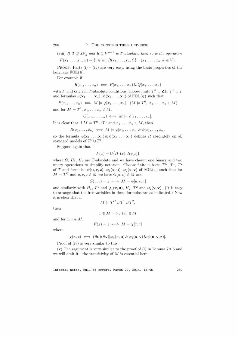
280 7. The constructible universe
(viii) If T ⊇ ZF−g and R ⊆ V n+1 is T -absolute, then so is the operation
F (x1, . . . , xn, w) = t ∈ w : R(x1, . . . , xn, t) (x1, . . . , xn, w ∈ V ).
Proof. Parts (i) – (iv) are very easy, using the basic properties of thelanguage FOL(∈).
For example if
R(x1, . . . , xn) ⇐⇒ P (x1, . . . , xn)&Q(x1, . . . , xn)
with P and Q given T -absolute conditions, choose finite T 0 ⊆ ZF, T 1 ⊆ Tand formulas ϕ(x1, . . . ,xn), ψ(x1, . . . ,xn) of FOL(∈) such that
P (x1, . . . , xn) ⇐⇒ M |= ϕ[x1, . . . , xn] (M |= T 0, x1, . . . , xn ∈ M)
and for M |= T 1, x1, . . . , xn ∈ M ,
Q(x1, . . . , xn) ⇐⇒ M |= ψ[x1, . . . , xn].
It is clear that if M |= T 0 ∪ T 1 and x1, . . . , xn ∈ M , then
R(x1, . . . , xn) ⇐⇒ M |= ϕ[x1, . . . , xn] &ψ[x1, . . . , xn],
so the formula ϕ(x1, . . . ,xn)&ψ(x1, . . . ,xn) defines R absolutely on allstandard models of T 0 ∪ T 1.
Suppose again that
F (x) = G(H1(x),H2(x)
)
where G, H1, H2 are T -absolute and we have chosen one binary and twounary operations to simplify notation. Choose finite subsets TG, T 1, T 2
of T and formulas ψ(u,v, z), ϕ1(x,u), ϕ2(x,v) of FOL(∈) such that forM |= TG and u, v, z ∈ M we have G(u, v) ∈ M and
G(u, v) = z ⇐⇒ M |= ψ[u, v, z]
and similarly with H1, T 1 and ϕ1(x,u), H2, T 2 and ϕ2(x,v). (It is easyto arrange that the free variables in these formulas are as indicated.) Nowit is clear that if
M |= TG ∪ T 1 ∪ T 2,
thenx ∈ M =⇒ F (x) ∈ M
and for x, z ∈ M ,F (x) = z ⇐⇒ M |= χ[x, z]
where
χ(x, z) ⇐⇒ (∃u)(∃v)[ϕ1(x,u)&ϕ2(x,v)&ψ(u,v, z)].
Proof of (iv) is very similar to this.(v) The argument is very similar to the proof of (i) in Lemma 7A.6 and
we will omit it—the transitivity of M is essential here.
Informal notes, full of errors, March 29, 2014, 15:45 280
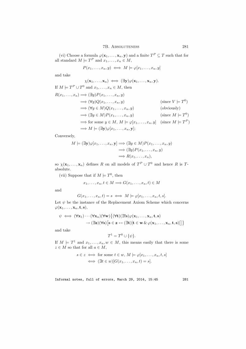
7B. Absoluteness 281
(vi) Choose a formula ϕ(x1, . . . ,xn,y) and a finite TP ⊆ T such that forall standard M |= TP and x1, . . . , xn ∈ M ,
P (x1, . . . , xn, y) ⇐⇒ M |= ϕ[x1, . . . , xn, y]
and takeχ(x1, . . . ,xn) ⇐⇒ (∃y)ϕ(x1, . . . ,xn,y).
If M |= TP ∪ T 0 and x1, . . . , xn ∈ M , then
R(x1, . . . , xn) =⇒ (∃y)P (x1, . . . , xn, y)
=⇒ (∀y)Q(x1, . . . , xn, y) (since V |= T 0)
=⇒ (∀y ∈ M)Q(x1, . . . , xn, y) (obviously)
=⇒ (∃y ∈ M)P (x1, . . . , xn, y) (since M |= T 0)
=⇒ for some y ∈ M , M |= ϕ[x1, . . . , xn, y] (since M |= TP )
=⇒ M |= (∃y)ϕ[x1, . . . , xn,y];
Conversely,
M |= (∃y)ϕ[x1, . . . , xn,y] =⇒ (∃y ∈ M)P (x1, . . . , xn, y)
=⇒ (∃y)P (x1, . . . , xn, y)
=⇒ R(x1, . . . , xn),
so χ(x1, . . . ,xn) defines R on all models of TP ∪ T 0 and hence R is T -absolute.
(vii) Suppose that if M |= T 0, then
x1, . . . , xn, t ∈ M =⇒ G(x1, . . . , xn, t) ∈ M
andG(x1, . . . , xn, t) = s ⇐⇒ M |= ϕ[x1, . . . , xn, t, s].
Let ψ be the instance of the Replacement Axiom Scheme which concernsϕ(x1, . . . ,xn, t, s),
ψ ⇐⇒ (∀x1) · · · (∀xn)(∀w)(∀t)(∃!s)ϕ(x1, . . . ,xn, t, s)
→ (∃z)(∀s)[s ∈ z ↔ (∃t)[t ∈ w&ϕ(x1, . . . ,xn, t, s)]
]
and takeT 1 = T 0 ∪ ψ.
If M |= T 1 and x1, . . . , xn, w ∈ M , this means easily that there is somez ∈ M so that for all a ∈ M ,
s ∈ z ⇐⇒ for some t ∈ w, M |= ϕ[x1, . . . , xn, t, s]
⇐⇒ (∃t ∈ w)[G(x1, . . . , xn, t) = s].
Informal notes, full of errors, March 29, 2014, 15:45 281

282 7. The constructible universe
Since M |= T 0 and hence M is closed under G, this implies that in fact
z = G(x1, . . . , xn, t) : t ∈ w= F (x1, . . . , xn, w),
hence M is closed under F . Moreover, taking
χ(x1, . . . ,xn,w, z) ⇐⇒ (∀s)[s ∈ z ↔ (∃t)[t ∈ w&ϕ(x1, . . . ,xn, t, s)]
],
is is clear that
F (x1, . . . , xn, w) = z ⇐⇒ M |= χ[x1, . . . , xn, w, z],
so F is T absolute.The argument with m > 1 is similar.(viii) Let
G(x1, . . . , xn, w, t) =
t if R(x1, . . . , xn, t),w if ¬R(x1, . . . , xn, t).
This is T -absolute by (ii) and then by the hypothesis that T ⊇ ZF−g, and(vii) (and (ii) again), the operation
F (x1, . . . , xn, w) = G(x1, . . . , xn, w, t) : t ∈ w ∩ w
is also T -absolute. Clearly
s ∈ F (x1, . . . , xn, w) ⇐⇒ s ∈ w &R(x1, . . . , xn, s)
∨ [s = w &w ∈ w &(∃t)¬R(x1, . . . , xn, t)];
and since w ∈ V so w /∈ w,
s ∈ F (x1, . . . , xn, w) ⇐⇒ s ∈ w &R(x1, . . . , xn, s)
as required. aCorollary 7B.4. The notions #1 – #21 of Theorem 6C.2 are all ZF−g-
absolute.
Proof is routine using the theorem and we will skip it. aBefore proceeding to show the ZF−g-absoluteness of several other notions,
it will be instructive to notice that many natural and useful notions are noteven ZFC-absolute, cf. Problem x7.1∗. Roughly speaking, no notion relatedto cardinality is ZFC-absolute.
The next result is fundamental.
Theorem 7B.5 (Mostowski’s Theorem). The condition
WF(r) ⇐⇒ r is a wellfounded relation
is ZF−g-absolute.
Informal notes, full of errors, March 29, 2014, 15:45 282

7B. Absoluteness 283
Proof. Put
P (r, x) ⇐⇒ Relation(r) & [x = ∅ ∨ (∃t ∈ x)(∀s ∈ x)〈〈s, t〉〉 /∈ r].
Clearly P is ZF−g-absolute and
WF(r) ⇐⇒ (∀x)P (r, x).
Similarly, let
Q(r, f) ⇐⇒ Relation(r)& [f is a rank function for r]⇐⇒ Relation(r) & f : Field(r) → ON
& (∀x, y ∈ Field(r))[x <r y =⇒ f(x) ∈ f(y)].
Again Q is ZF−g-absolute (using the fact that ON is definable by a Σ0
formula) andWF(r) ⇐⇒ (∃f)Q(r, f).
Hence
(∀r)[(∀x)P (x, r) ⇐⇒ (∃f)Q(r, f)
].(∗)
This equivalence is Problem x6.26, and it can be proved in ZF−g.Let θ be the formal sentence which expresses (∗), so that ZF−g ` θ. Let
T ∗ ⊆ ZF−g be the finite set of ZF−g axioms used in the proof of θ, so thatθ is true in all models of T ∗, including all the standard models. Let T 0,T 1 be finite subsets of ZF−g such that P and Q are absolute for standardmodels of T 0 and T 1 respectively. It follows that if M is a standard modelof T 0 ∪ T 1 ∪ T ∗, then for r ∈ M
(∀x ∈ M)P (x, r) ⇐⇒ (∃f ∈ M)Q(r, f).(∗∗)Now part (vi) of 7B.3 implies that WF(r) is ZF−g-absolute. a
Mostowski’s proof is simple but typically metamathematical and gener-ally causes uneasiness to people who encounter it for the first time. Thesubtle part of it is that we do not need to identify the specific instancesof replacement needed to prove θ—we only need to notice that there areonly finitely many of them, and then put them in T ∗. In this instance,we could probably pinpoint these instances, but that would be the wrongway to go about understanding the proof: because this sort of argument isused repeatedly, in ever more complex situations where chasing the specificinstances of replacement used would be practically impossible. The argu-ment rests on the fact that proofs are finite, so that for any formal τ -theoryT and any τ -sentence φ,
T ` φ=⇒ (∃ finite T0 ⊆ T )[T0 ` φ].
The same kind of metamathematical argument is needed in the proof ofthe next result.
Informal notes, full of errors, March 29, 2014, 15:45 283

284 7. The constructible universe
Theorem 7B.6 (Absoluteness of ordinal recursion). Suppose the oper-ation G : V n+1 → V is ZF−g-absolute, and let
F : ON× V n → V
be the unique operation satisfying
F (ξ, x1, . . . , xn) = G(〈〈η, F (η, x1, . . . , xn)〉〉 : η < ξ, x1, . . . , xn
);
then F is also ZF−g-absolute.
Proof. Assume G is absolute for all standard models of T 0 ⊆ ZF−g.Go back to the proof of Theorem 6C.16 to recall that F is defined by anexpression of the form
F (ξ, x1, . . . , xn) = w ⇐⇒ (∃h)P (ξ, x1, . . . , xn, h)&Function(h)
& ξ ∈ Domain(h)&h(ξ) = w,where P is easily absolute for all models of T 0. Moreover, we can prove
(∀ξ, x1, . . . , xn)(∃h)P (ξ, x1, . . . , xn, h)
using only finitely many additional instances of the Axiom Scheme of Re-placement, say those in T 1 ⊆ ZF−g. Thus for every standard model M ofT 0∪T 1 and ξ, x1, . . . , xn in M we have (∃h ∈ M)P (ξ, x1, . . . , xn, h), whichimplies immediately that M is closed under F .
We can also prove easily in ZF−g (using only some finite T 2 ⊆ ZF−g) that
(∀ξ, x1, . . . , xn, w)(∃h)[P (ξ, x1, . . . , xn, h)&Function(h)
& ξ ∈ Domain(h)&h(ξ) = w] ⇐⇒ (∀h)[[P (ξ, x1, . . . , xn, h)
&Function(h)& ξ ∈ Domain(h)] =⇒ h(ξ = w]
;
thus by part (vi) of 7B.3, the condition
R(ξ, x1, . . . , xn, w) ⇐⇒ F (ξ, x1, . . . , xn) = w
is ZF−g-absolute and so F is ZF−g-absolute. aA special case of definition by recursion on ON is simple recursion on ω.
Corollary 7B.7. Suppose F (k, x1, . . . , xn) satisfies the recursion
F (0, x1, . . . , xn) = G(x1, . . . , xn)
F (k + 1, x1, . . . , xn) = G(F (k, x1, . . . , xn), k, x1, . . . , xn
)
where G1 and G2 are ZF−g-absolute. Then F is also ZF−g-absolute.
Informal notes, full of errors, March 29, 2014, 15:45 284

7C. The basic facts about L 285
Proof. Define
G(f, k, x1, . . . , xn) =
G1(x1, . . . , xn) if m = 0,G2
(f(k − 1, x1, . . . , xn), k − 1, x1, . . . , xn
)if k ∈ ω, k 6= 0,
0 otherwise
and verify easily that G is ZF−g-absolute and F is definable from G as inthe theorem. a
Corollary 7B.8. All the conditions and operations #1 – #40 in Theo-rems 6C.2 and 7A.1 are ZF−g-absolute.
Proof. Go back and reread the proofs of these theorems keeping inmind the results of this section. a
7C. The basic facts about L
Let us start by collecting in one theorem the basic absoluteness factsabout the constructible hierarchy that follow from the results of the pre-ceding section.
Theorem 7C.1. (i) The operation ξ 7→ Lξ and the binary conditionx ∈ Lξ are both ZF−g-absolute.
(ii) There is a canonical wellordering of L, x ≤L y which is ZF−g-absoluteand such that
y ∈ Lξ & x ≤L y =⇒ x ∈ Lξ.
(iii) The operation (ξ, A) 7→ Lξ(A) and the ternary condition x ∈ Lξ(A)are both ZF−g-absolute.
(iv) The conditions x ∈ L and x ∈ L(A) are both absolute for inner modelsof some finite subset T 0 ⊆ ZF−g.
Proof. (i) and (ii) follow immediately from the definitions, 7B.8, 7B.6and of course, the basic closure properties of ZF−g-absoluteness listed in 7B.3.Part (ii) also follows easily by examining the proof of 7A.8.
To prove (iv), let ϕL(x, ξ) be a formula of FOL(∈) by (i) such that forsome finite T 0 ⊆ ZF−g and any standard M
x ∈ Lξ ⇐⇒ M |= ϕL[x, ξ] (M standard, M |= T 0),(7C-12)
and set ψL(x) :≡ (∃ξ)ϕL(x, ξ). If M is an inner model of T 0 so thatM |= T 0 and M contains all the ordinals, then for x ∈ M ,
x ∈ L ⇐⇒ for some ξ, x ∈ Lξ
⇐⇒ for some ξ ∈ M , M |= ϕL[x, ξ]
⇐⇒ M |= ψL[x].
Informal notes, full of errors, March 29, 2014, 15:45 285

286 7. The constructible universe
The argument for x ∈ L(A) is similar. aWe are now in a position to prove (7B-8), that L “believes” that every
set is constructible.Fix once and for all a formula ϕL(x, ξ) and a finite T 0 ⊂ ZF−g so that (7C-12)
holds and let “V = L” abbreviate the formal sentence of FOL(∈) whichsays that every set is constructible using this formula,
V = L :≡ (∀x)(∃ξ)ϕL(x, ξ).(7C-13)
We also construct a similar formula V = L(a) with a free variable a whichsays that “every set is constructible from a”.
Theorem 7C.2. (i) L |= V = L.(ii) For each grounded set A, L(A),a := A |= V = L(a).
Proof. Compute:
L |= V = L ⇐⇒ L |= (∀x)(∃ξ)ϕL(x, ξ)
⇐⇒ for each x ∈ L, there exists ξ ∈ L, L |= ϕL(x, ξ)⇐⇒ for each x ∈ L, there exists ξ ∈ L, x ∈ Lξ,
and the last assertion is true by the definition of L and the fact that itcontains all the ordinals. a
This is a very basic result about L. One of its applications is that itallows us to prove theorems about L without constant appeal to meta-mathematical results and methods: we simply assume V = L in additionto the axioms of ZF−g and any consequence of these assumptions must holdin L.
We also put down for the record the result about the Axiom of Choicein L which we discussed in the beginning of Section 7B.
Theorem 7C.3. There is a formula ψL(x,y) of FOL(∈) such that
L |= “(x, y) : ψL(x, y) is a wellordering of V ”.
In particular, L |= AC.
Proof. If ψ∗ is the formal sentence of FOL(∈) expressing the symbol-ized English in quotes, then by 7A.8 and the fact that L |= ZF−g,
L |= V = L → ψ∗
while by 7C.2 we have L |= V = L. aFor the Generalized Continuum Hypothesis we need another basic fact
about L which is also proved by absoluteness arguments. Its proof requirestwo general facts, not particularly related to L, which could have beenincluded in Chapter 6.
The first of these is the natural generalization of Theorem 2B.1 to un-countable structures.
Informal notes, full of errors, March 29, 2014, 15:45 286
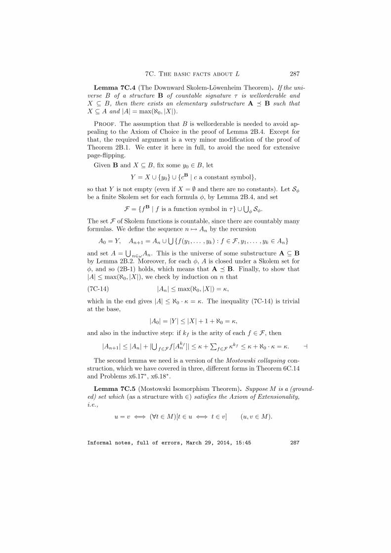
7C. The basic facts about L 287
Lemma 7C.4 (The Downward Skolem-Lowenheim Theorem). If the uni-verse B of a structure B of countable signature τ is wellorderable andX ⊆ B, then there exists an elementary substructure A ¹ B such thatX ⊆ A and |A| = max(ℵ0, |X|).
Proof. The assumption that B is wellorderable is needed to avoid ap-pealing to the Axiom of Choice in the proof of Lemma 2B.4. Except forthat, the required argument is a very minor modification of the proof ofTheorem 2B.1. We enter it here in full, to avoid the need for extensivepage-flipping.
Given B and X ⊆ B, fix some y0 ∈ B, let
Y = X ∪ y0 ∪ cB | c a constant symbol,so that Y is not empty (even if X = ∅ and there are no constants). Let Sφ
be a finite Skolem set for each formula φ, by Lemma 2B.4, and set
F = fB | f is a function symbol in τ ∪⋃φ Sφ.
The set F of Skolem functions is countable, since there are countably manyformulas. We define the sequence n 7→ An by the recursion
A0 = Y, An+1 = An ∪⋃f(y1, . . . , yk) : f ∈ F , y1, . . . , yk ∈ An
and set A =⋃
n∈ωAn. This is the universe of some substructure A ⊆ Bby Lemma 2B.2. Moreover, for each φ, A is closed under a Skolem set forφ, and so (2B-1) holds, which means that A ¹ B. Finally, to show that|A| ≤ max(ℵ0, |X|), we check by induction on n that
|An| ≤ max(ℵ0, |X|) = κ,(7C-14)
which in the end gives |A| ≤ ℵ0 · κ = κ. The inequality (7C-14) is trivialat the base,
|A0| = |Y | ≤ |X|+ 1 + ℵ0 = κ,
and also in the inductive step: if kf is the arity of each f ∈ F , then
|An+1| ≤ |An|+ |⋃ f∈Ff [Akfn ]| ≤ κ +
∑f∈F κkf ≤ κ + ℵ0 · κ = κ. a
The second lemma we need is a version of the Mostowski collapsing con-struction, which we have covered in three, different forms in Theorem 6C.14and Problems x6.17∗, x6.18∗.
Lemma 7C.5 (Mostowski Isomorphism Theorem). Suppose M is a (ground-ed) set which (as a structure with ∈) satisfies the Axiom of Extensionality,i.e.,
u = v ⇐⇒ (∀t ∈ M)[t ∈ u ⇐⇒ t ∈ v] (u, v ∈ M).
Informal notes, full of errors, March 29, 2014, 15:45 287

288 7. The constructible universe
Let dM : M → dM [M ] be the Mostowski surjection of ∈¹M , so that
dM (u) = dM (v) : v ∈ M ∩ u (u ∈ M).(7C-15)
Then M = dM [M ] is a transitive set, dM : M ½→M is an ∈-isomorphismof (M,∈) with (M,∈), and if y ⊆ M is transitive, then dM (t) = t for everyt ∈ y.
Proof. The unique function dM : M → V satisfying (7C-15) is de-fined by wellfounded recursion, and its image is a transitive set, directlyfrom (7C-15): because if s ∈ dM (u) for some u ∈ M , then
s = dM (v) = dM (t) : t ∈ M ∩ vfor some v ∈ M ∩ u and so s ⊆ dM [M ].
To prove that dM is an injection, assume not and let u be an ∈-minimalcounterexample, so that for some v ∈ M , v 6= u,
dM (u) = dM (s) : s ∈ M ∩ u = dM (t) : t ∈ M ∩ v = dM (v).
It follows that if s ∈ M ∩ u, then dM (s) = dM (t) for some t ∈ M ∩ v,so that by the choice of u, s = t ∈ M ∩ v. Similarly, if t ∈ M ∩ v, thent ∈ M ∩ u. So M ∩ u = M ∩ v, and since M satisfies extensionality, u = v,which contradicts our assumption.
Finally, if dM is not the identity on some transitive y ⊆ M , choose an∈-minimal t ∈ y such that dM (t) 6= t and compute:
dM (t) = dM (s) : s ∈ t (because t ⊆ y ⊆ M)= s : s ∈ t (by the choice of t)= t (because t ⊆ y ⊆ M),
which again contradicts our assumption. aIn the context of the metamathematics of set theory (especially the study
of L and other inner models), “the Mostowski Collapsing Lemma” mostlikely refers to this theorem. We used a different (standard but less com-mon) name for it here, to avoid confusion. In any case, these two results(and Problems x6.17∗, x6.18∗) have different applications, but they areproved by the same method and they are all significant.
Theorem 7C.6 (The Condensation Lemma). There is a finite set ofsentences T 0 ⊂ ZF−g such that with
TL = T 0 ∪ V = Lthe following hold.
(i) L |= TL.(ii) If A is a transitive set and A |= TL, then A = Lλ for some limit
ordinal λ.
Informal notes, full of errors, March 29, 2014, 15:45 288

7C. The basic facts about L 289
(iii) For every infinite ordinal ξ and every set x ∈ L such that x ⊆ Lξ,there is some ordinal λ such that
ξ ≤ λ < ξ+, Lλ |= TL, and x ∈ Lλ.
Proof. Choose T 0 so that the operations ξ 7→ ξ + 1, ξ 7→ Lξ, areabsolute for the standard models of T 0 and the condition x ∈ Lξ is definedon all standard models of T 0 by the specific formula ϕL(x, ξ) which weused to construct the sentence V = L.
Clearly L |= TL.If A is a transitive set and A |= TL, let
λ = least ordinal not in A
and notice that λ is a limit ordinal, since A is closed under the successoroperation. Now
ξ < λ =⇒ Lξ ∈ A,
by the absoluteness of ξ 7→ Lξ, so
Lλ =⋃
ξ<λ Lξ ⊆ A.
On the other hand, A |= V = L, so that
for each x ∈ A, there exists ξ ∈ A, A |= ϕL[x, ξ]
i.e., (by the absoluteness of ϕL(x, ξ)), A ⊆ Lλ.To prove (iii) suppose x ⊆ Lξ and x ∈ Lζ—where ζ may be a much
larger ordinal than ξ. Using the Reflection Theorem 6D.7 on the hierarchyLη : η ∈ ON and the fact that L |= TL, choose µ > max(ζ, ξ) such thatLµ |= TL. Now x ∈ Lµ and Lµ |= TL.
By the Downward Skolem-Lowenheim Theorem 7C.4 applied to the (well-orderable) structure (Lµ,∈), we can find an elementary substructure
(M,∈) ¹ (Lµ,∈)
such that Lξ ⊆ M , x ∈ M and |M | = |Lξ| = |ξ| by x7.6. Since (M,∈)is elementarily equivalent with (Lµ,∈), it satisfies in particular the Exten-sionality Axiom, so by the Mostowski Isomorphism Theorem 7C.5, there isa transitive set M and an ∈-isomorphism
d : M ½→M.
Moreover, since the transitive set y = Lξ ∪ x ⊆ M , d is the identity ony and hence x = d(x) ∈ M . Now (Lµ,∈) |= TL and therefore the elemen-tarily equivalent structure (M,∈) |= TL, so that the isomorphic structure(M,∈) |= TL; by (ii) then,
M = Lλ
for some λ and of course, λ < ξ+, since |M | = |ξ|. a
Informal notes, full of errors, March 29, 2014, 15:45 289

290 7. The constructible universe
From this key theorem we get immediately the Generalized ContinuumHypothesis for L.
Corollary 7C.7 (ZF). If V = L, then for each cardinal λ, 2λ = λ+.
Proof. By the theorem, if V = L, then P(λ) ⊆ Lλ+ , and hence
|P(λ)| ≤ |Lλ+| = λ+. aWe should point out that the models L(A) need not satisfy either the
Axiom of Choice or the Continuum Hypothesis. For example, if in V truly2ℵ0 > ℵ1, then there is some surjection
π : N ³ ℵ2
and obviouslyL
(〈〈α, π(α)〉〉 : α ∈ N) |= 2ℵ0 ≥ ℵ2.
As another application of the basic Theorem 7C.1, we obtain intrinsiccharacterizations of the models L, L(A).
Theorem 7C.8. L is the smallest inner model of ZF−g and for each(grounded) set A, L(A) is the smallest inner model of ZF−g which con-tains A.
Proof. Suppose M is an inner model of ZF−g and A0 ∈ M . Since theoperation
(ξ,A) 7→ Lξ(A)
is ZF−g-absolute, M is closed under this operation; since A0 ∈ M and everyordinal ξ ∈ M , we have (∀ξ)[Lξ(A0) ∈ M ] so that L(A0) ⊆ M . a
We also put down for the record the relative consistency consequences ofof the theory of constructible sets:
Theorem 7C.9. If ZF is consistent, then so is the theory ZFg +V = L,and a fortiori the weaker theories ZFC, ZFC + GCH.
Proof. It is useful here to revert to the relativization notation of Defi-nition 6D.6. The key observation is that for any FOL(∈) formula φ,
if ZFg + V = L ` φ, then ZF ` (φ)L.(7C-16)
This is because ZF ` (ψ)L for every axiom ψ of ZFg by Theorem 7A.7;ZF ` (V = L)L by Theorem 7C.2; and, pretty trivially,
if ψ1, . . . , ψn ` ψ, then (ψ1)M , . . . , (ψn)M ` (ψ)M ,
for any definable class M , not just L. If ZF+V = L were inconsistent, thenZF+V = L ` χ & ¬χ for some χ for some χ, and then ZF ` (χ)L & ¬(χ)L,so that ZF would also be inconsistent. a
Informal notes, full of errors, March 29, 2014, 15:45 290

7D. ♦ 291
This is an example of a finitistic relative consistency proof : it can beformalized in a (very small) fragment of Peano arithmetic, but, more thanthat, it is generally recognized as a valid, constructive, combinatorial ar-gument which assumes nothing about infinite objects beyond the usualproperties of finite strings of symbols.
7D. ♦
Our (very limited) aim in this section is to introduce a basic principle ofinfinite combinatorics and prove that it holds in L. It was first formulatedby Jensen to prove that L satisfies several propositions which are indepen-dent of ZFC, but we will not go into this here beyond a brief comment atthe end: our main interest in ♦ is that its proof in L illustrates in a novelway many of the methods we have developed.
A guessing sequence (for ω1) is any ω1-sequence of functions on countableordinals
s = sξξ∈ω1 (sξ : ξ → ξ).(7D-17)
Definition 7D.1. ♦ : There exists a guessing sequence s = sξξ∈ω1
such that for every f : ω1 → ω1, there is at least one ξ > 0 such thatf ¹ξ = sξ.
The diamond principle seems weak, but the next Proposition shows thatit has considerable strength. For the proof, we will need to appeal to somesimple properties of pairing functions on ordinals which we will leave forProblem x7.12.
Proposition 7D.2 (ZFC). If ♦ holds, then there is a guessing sequencetξξ∈ω1 which guesses correctly ℵ1-many restrictions of every f : ω1 → ω1,i.e.,
|ξ : f ¹ξ = tξ| = ℵ1 (f : ω1 → ω1).
Proof. Let sξξ∈ω1 be a guessing sequence guaranteed by ♦, supposef : ω1 → ω1 is given, fix ζ < ω1, and set
hζ(η) = 〈f(η), ζ〉 so that f(η) = (hζ(η))0.
Let ξ(ζ) > 0 be such that
hζ ¹ξ(ζ) = sξ(ζ).
This means that for every η < ξ(ζ), f(η) = (sξ(ζ))0; and it implies imme-diately that the sequence
tξ(η) = (sξ(η))0 ≤ sξ(η) < ξ (ξ < ω1, η < ξ)
Informal notes, full of errors, March 29, 2014, 15:45 291

292 7. The constructible universe
guesses f ¹ ξ(ζ) correctly for every ζ. Moreover, these ordinals are alldistinct, since
(sξ(ζ)(0))1 = ζ,
so that we cannot have ξ(ζ1) = ξ(ζ2) > 0 when ζ1 6= ζ2. aIt is important in this proof, of course, to notice that the new guessing
sequence tξξ∈ω1 is defined directly from the one guaranteed by ♦, withoutreference to any specific f or ordinal ζ.
Corollary 7D.3 (ZFC). ♦ =⇒CH.
Proof. Fix a guessing sequence tξξ∈ω1 which guesses correctly ℵ1-many restrictions of every f : ω1 → ω1, and for each f : ω → ω apply itscharacteristic property to the extension f : ω1 → ω of f which is set = 0for ξ ≥ ω. Let ξ(f) be the least infinite ordinal such that f ¹ξ(f) = tξ(f);now ξ(f) determines f uniquely, so that the map f 7→ ξ(f) is an injectionof (ω → ω) into ω1 and establishes the Continuum Hypothesis. a
Theorem 7D.4 (ZFC). If V = L, then ♦.
Proof. We assume V = L and define sξ by recursion on ξ < ω1, startingwith (the irrelevant) s0 = ∅. For ξ > 0, let
(7D-18) sξ = the ≤L-least function h : ξ → ξ such thatfor every ζ < ξ, ζ 6= 0, h¹ζ 6= sζ ,
with the understanding that if no h with the required property exists, thensξ is the constant 0 on ξ. Recall that by our general convention about“indexed sequences”,
sξξ∈ω1 = s : ω1 → (ω1 → ω1),
i.e., s is a function, and sξ = s(ξ) for every ξ ∈ ω1.To prove that for every f : ω1 → ω1, this sequence s guesses correctly
f ¹ξ for at least one ξ > 0, assume that it does not, and let
(7D-19) f = the ≤L-least function h : ω1 → ω1 such thatfor every ζ < ω1, ζ > 0, h¹ζ 6= sζ .
Notice that by the Condensation Lemma, s, f ∈ Lω2 , cf. Problem x7.11.A set a ∈ Lω2 is definable (in Lω2) if there is a formula φ(x) such that
Lω2 |= (∃!x)φ(x) and Lω2 |= φ[a].
We let
M = a ∈ Lω2 : a is definable in Lω2.Lemma 1. M ≺ Lω2 |= ZF−g and ω, ω1, s, f ∈ M .
Informal notes, full of errors, March 29, 2014, 15:45 292

7D. ♦ 293
Proof. By Problem x7.10, Lω2 |= ZF−g, and so all ZF−g-absolute notionsare absolute for Lω2 . In particular, the usual definitions of ω, ω1 definethese sets in Lω2 and the formula which defines the canonical wellordering≤L is also absolute for Lω2 , and so we can interpret the definitions of s andf in Lω2 ; which means that s, f ∈ M .
To prove that M ≺ Lω2 by the basic test for elementary substructuresLemma 2A.3, it is enough to check that for every full extended formulaφ(x1, . . . ,xn,y) and all ~x = x1, . . . , xn ∈ M ,
if there exists some y ∈ Lω2 such that Lω2 |= φ[~x, y],
then there exists some z ∈ M such that Lω2 |= φ[~x, z].
This is immediate setting
z = the ≤L-least y ∈ Lω2 such that Lω2 |= φ[~x, y]. a (Lemma 1)
Let d : M ½→Lλ be the Mostowski isomorphism for M , so λ < ω1 and
d : M ½→Lλ |= ZF−g, (∀y)[TC(y) ⊂ M =⇒ d(y) = y].
Lemma 2. If F : Ln → L is a ZF−g-absolute operation, then
x1, . . . , xn ∈ M
=⇒F (x1, . . . , xn) ∈ M & d(F (x1, . . . , xn)) = F (d(x1), . . . , d(xn)).
Proof. Suppose φ(x1, . . . ,xn,y) defines F on every transitive model ofZF−g. In particular, Lω2 |= (∀~x)(∃!y)φ(~x,y), and so M |= (∀~x)(∃!y)φ(~x,y)which means that M is closed under F . Moreover, for x1, . . . , xn, y ∈ M ,
M |= φ[x1, . . . , xn, y] ⇐⇒ Lλ |= φ[d(x1), . . . , d(xn), d(y)]
⇐⇒ F (d(x1), . . . , d(xn)) = d(y),
the last because Lλ |= ZF−g and so φ(~x,y) also defines F on it.a (Lemma 2)Lemma 2 implies in particular that if g ∈ M , then Domain(g) ∈ M and
for every a ∈ Domain(g) ∩M ,
d(g(a)) ∈ M and d(g(a)) = d(g)(d(a)),(7D-20)
simply because the operations
g 7→ Domain(g), (g, a) 7→ g(a)
are ZF−g-absolute. In particular, if ξ < ω1, then
ξ ∈ M =⇒ f(ξ), sξ ∈ M, and [η, ξ ∈ M & η < ξ] =⇒ sξ(η) ∈ M.
Lemma 3. If ξ is countable and ξ ∈ M , then d(ξ) = ξ.
Informal notes, full of errors, March 29, 2014, 15:45 293

294 7. The constructible universe
Proof. We can prove in ZF−g that every countable ordinal ξ is the imageof some g : ω→→ ξ, and so if ξ is definable in Lω2 , then so is
g = the ≤L-least g : ω→→ ξ.
It follows that every η < ξ is g(n) for some n ∈ ω and hence definable inLω2 ; and then ξ + 1 = TC(ξ) ⊂ M , and so the Mostowski isomorphism dis the identity on ξ + 1 and gives d(ξ) = ξ. a (Lemma 3)
Lemma 4. If µ = d(ω1), then d(f) = f ¹µ and for ξ < µ, d(sξ) = sξ.
Proof. The key observation is that
ξ < µ ⇐⇒ [ξ ∈ M & ξ < ω1].
This is because using Lemma 3,
ξ ∈ M & ξ < ω1 =⇒ ξ = d(ξ) & d(ξ) < d(ω1) = µ,
and on the other hand,
ξ < µ =⇒ (∃η)[η ∈ M & η < ω1 & ξ = d(η)]
=⇒ (∃η)[η ∈ M & η < ω1 & ξ = η] =⇒ ξ ∈ M & ξ < ω1.
In particular, ξ < µ =⇒ d(ξ) = ξ, and since f ∈ M and f(ξ) < ω1,by (7D-20),
ξ < µ =⇒ f(ξ) = d(f(ξ)) = d(f)(d(ξ)) = d(f)(ξ),
i.e., d(f) = f ¹µ. Similarly,
η < ξ < µ =⇒ sξ(η) = d(sξ(η)) = d(sξ)(η),
and so for ξ < µ, d(sξ) = sξ. a (Lemma 4)We now consider the definition (7D-18) of sµ: it is the unique g : µ → µ
which satisfies the condition
φ[g, µ] ≡ g is the ≤L-least h : µ → µ such thatfor every ζ < µ, ζ > 0, h¹µ 6= sζ .
Since the formula φ(x,y) is ZF−g-absolute and sµ ∈ Lω2 , this implies that
sµ is the unique g such that Lω2 |= φ[g, µ].
By the definition (7D-19) of f and the same reasoning,
f is the unique h such that Lω2 |= φ[h,ℵ1];
and so M |= φ[f,ℵ1], hence Lλ |= φ[d(f), µ]. We now appeal again to thefact that φ(x,y) is ZF−g-absolute: since Lλ |= ZF−g, N |= φ[d(f), µ] for everytransitive N |= ZF−g which contains d(f) and µ, and in particular,
Lω2 |= φ[d(f), µ].
Informal notes, full of errors, March 29, 2014, 15:45 294

7D. ♦ 295
So sµ = d(f) and d(f) = f ¹µ by Lemma 4, which contradicts the choiceof f . a
How large can we make the set of correct guesses
ξ > 0 : f ¹ξ = tξfor every f : ω1 → ω1 by choosing cleverly the guessing sequence tξξ∈ω1?We cannot (rather trivially) insure that this set is always a closed un-bounded subset of ω1, cf. Problem x7.13, but we can insure the next, bestpossible result.
A set C ⊆ ω1 is stationary if it intersects every closed, unbounded subsetof ω1.
Theorem 7D.5 (ZFC). If ♦ holds, then there is a guessing sequencetξξ∈ω1 such that for every f : ω1 → ω1 the set ξ > 0 : f ¹ ξ = tξ isstationary.
Proof is left for Problem x7.14∗. aThis is about the strongest version of ♦ which is close to the formulation
we chose as “primary”, but there are many other equivalent propositions,each with its own uses and applications.
The Suslin Hypothesis. The order (R,≤) on the real numbers can becharacterized up to similarity by the following two properties which do notrefer to the field structure of R:(1) (X,≤) is a linear ordering with no least or greatest element; it is dense
in itself, i.e., a < b=⇒ (∃x)[a < x < b]; and it is order complete, i.e.,every set X ⊆ (a, b) contained in an open interval has a least upperbound and a greatest lower bound.
(2) (X,≤) is separable, i.e., there is a countable set Q ⊂ X which inter-sects every open interval (a, b).
Suslin’s question was whether (2) can be replaced by the weaker(2′) There is no uncountable set of disjoint open intervals in X.
Call (X,≤) a Suslin line if it satisfies (1) and (2′) but not (2).Suslin Hypothesis. There is no Suslin line.The Suslin Hypothesis is neither provable nor disprovable in ZFC. Both
of these results were established by forcing techniques soon after Cohen’s in-troduction of the method in 1963, and they were among the most importantearly results in forcing—especially the consistency of Suslin’s Hypothesis.Soon afterwards Jensen proved that there is a Suslin line in L. His proof iscombinatorial complex (and uses the intermediate notion of a Suslin tree)but the main tool for it was the proof of ♦ in L. It is fair to say thatJensen’s theorem was the first, substantial result which started the moderndevelopment of combinatorial set theory, in and outside L.
Informal notes, full of errors, March 29, 2014, 15:45 295

296 7. The constructible universe
7E. L and Σ12
We finish this Chapter with some basic results of Shoenfield which relatethe constructible universe to the analytical hierarchy developed in Sec-tions ?? and ??. We will assume for simplicity ZFC as the underlyingtheory, although most of what we will prove can be established without thefull versions of either the powerset axiom or the axiom of choice.
Theorem 7E.1. (i) The set N ∩L of constructible members of Bairespace is Σ1
2.
(ii) The restriction of ≤L to N is a Σ12-good wellordering of N ∩ L; i.e.,
it is a Σ12 relation on N , and if P ⊆ ωn × N ν is in Σ1
2, then so arethe relations
Q(α, ~x, ~β) ⇐⇒ α ∈ L & (∃β ≤L α)P (β, ~x, ~β),
R(α, ~x, ~β) ⇐⇒ α ∈ L & (∀β ≤L α)P (β, ~x, ~β).
(iii) If N ⊆ L, then N admits a Σ12-good wellordering of rank ℵ1.
Proof. (i) is an easy consequence of (ii), but it is instructive to show (i)first.
First of all, we claim that if TL is the finite set of sentences in theCondensation Lemma 7C.6, then
α ∈ L ⇐⇒ there exists a countable, transitive set A such that(A,∈) |= TL and α ∈ A.
(7E-21)
The implication (⇐=) in (7E-21) is immediate, because by Theorem 7C.6,if (A,∈) |= TL, then A = Lλ for some ordinal λ. For the other direction,notice that (as a set of pairs of natural numbers), each α is a subset of Lω
so by (iii) of 7C.6
α ∈ L ⇐⇒ for some countable λ, α ∈ Lλ and Lλ |= TL.
The key idea of the proof is that the structures of the form (A,∈) withcountable transitive A can be characterized up to isomorphism by the ver-sion for sets of the Mostowski Collapsing Lemma in Problem x6.17∗. Infact, if (M,E) is any structure with countable M and E ⊆ M ×M , thenby x6.17∗, immediately
(M,E) is isomorphic with some (A,∈) where A is countable, transitive
⇐⇒ E is wellfounded and (M,E) |=“axiom of extensionality”;
Informal notes, full of errors, March 29, 2014, 15:45 296

7E. L and Σ12 297
thus
α ∈ L ⇐⇒ there exists a countable, wellfounded structure(M, E) such that (M,E) |= “axiom ofextensionality”, (M,E) |= TL and α ∈ M = theunique transitive set such that (M,E) is isomorphicwith (M,∈).
(7E-22)
To see how to express the last condition in a model-theoretic way, recallthat the condition “α ∈ N” is ZF−g-absolute and choose some ϕ0(α) suchthat for all transitive models M of some finite T0 ⊆ ZF−g,
α ∈ N ⇐⇒ M |= ϕ0[α].
Next define for each integer n a formula ψn(x) which asserts that x = n,by the recursion
ψ0(x) ⇐⇒ x = 0,
ψn+1(x) ⇐⇒ (∃y)[ψn(y)&x = y ∪ y]
and for each n, m, let
ψn,m(α) :≡ (∃x)(∃y)[ψn(x)&ψm(y)& 〈〈x,y〉〉 ∈ α].
It follows that
α ∈ L ⇐⇒ there exists a countable, wellfounded structure(M, E) such that (M,E) |= “axiom ofextensionality”, (M,E) |= TL and for some a ∈ M ,(M, E) |= ϕ0[a] and for all n, m,α(n) = m ⇐⇒ (M, E) |= ψn,m[a].
(7E-23)
Let
f(m,n) = the code of the formula ψm,n(α),
so that f is obviously a recursive function. Let also k0 be the code of theconjunction of the sentences in TL and the Axiom of Extensionality and letk1 be the code of the formula ϕ0(α) which defines α ∈ N ; we are assumingthat both in ψm,n(α) and in ϕ0(α), the free variable α is actually the firstvariable v0. It is now clear that with u = 〈2〉 the code of the vocabulary
Informal notes, full of errors, March 29, 2014, 15:45 297

298 7. The constructible universe
for structures with just one binary relation,
α ∈ L ⇐⇒ (∃β)
Sat(u, β, k0, 1)
& (t, s) : (β)0(t) = (β)0(s) = 1& (β)1(〈t, s〉) = 1is wellfounded
& (∃a)[Sat(u, β, k1, 〈a〉)
& (∀n)(∀m)[α(n) = m ⇐⇒ Sat
(u, β, f(n,m), 〈α〉)]
]
which implies directly that L∩N is Σ12, using the fact that wellfoundedness
is Π11.
To prove (ii), let ψL(v0,v1) be a formula which defines the canonicalwellordering of L absolutely on all transitive models of some finite TL
1 ⊆ZF−g (by (ii) of 7C.1) and let SL ⊆ ZF−g be finite and large enough to includeTL
1 , TL, the Axiom of Extensionality and the set T0 of part (i), chosen sothat ϕ0(α) defines α ∈ N on all transitive models of T0. Using the keyfact
α ∈ Lξ &β ≤L α =⇒ α ∈ Lξ
and Mostowski collapsing as above, we can verify directly that for α ∈ Land arbitrary P ⊆ N ×Z (with Z = ωn ×N ν),
(∀β ≤L α)P (β, z)⇐⇒ there exists a countable, wellfounded structure
(M,E) |= SL and some a ∈ M such that (M, E) |= ϕ0[a]and (∀n)(∀m)[α(n) = m ⇐⇒ (M,E) |= ψn,m[a]]and (∀b)
(M,E) |= ϕ0[b] &ψL(b, a) =⇒
(∃β)[(∀n)(∀m)[β(n) = m
⇐⇒ (M, E) |= ψn,m[b]] &P (β, z)]
.
If P is Σ12, then it is easy to see that this whole expression on the right
leads to a Σ12 condition by coding the structures (M, E) by irrationals as
above—the key being that the universal quantifier ∀β has been turned tothe number quantifier ∀b. a
We put down the argument for (i) in considerable detail, because itillustrates a very useful technique for making analytical computations ofconditions defined by set-theoretic constructions. For the next result we willdo the opposite, i.e., we will give a set-theoretic construction for Σ1
2 subsetsof ωn ×N ν which will establish that (as conditions) they are absolute forL.
We show first a basic result, which has many applications beyond ourimmediate concern:
Informal notes, full of errors, March 29, 2014, 15:45 298

7E. L and Σ12 299
Theorem 7E.2 (Shoenfield’s Lemma). If A ⊆ N is Σ12, then there ex-
ists a ZF−g-absolute operation
ξ 7→ T ξ
which assigns to each ordinal ξ ≥ ω a tree T ξ on ω × ξ such that thefollowing holds, when λ is any uncountable ordinal:
α ∈ A ⇐⇒ (∃ξ ≥ ω)[T ξ(a) is not wellfounded]
⇐⇒ (∃ξ ≥ ω)[ξ < ω1 & T ξ(α) is not wellfounded]
⇐⇒ Tλ(α) is not wellfounded.
Proof. Choose a recursive, monotone R so that
α ∈ A ⇐⇒ (∃β)(∀γ)(∃t)R(α(t), β(t), γ(t)
),
and for all α(n), β(n), γ(n),(¬R(α(t), β(t), γ(t)) & s < t
)=⇒¬R(α(s), β(s), γ(s)).
It follows that for each α, β, the set of sequences
Sα,β =(c0, . . . , cs−1) : (∀t < s)¬R
(α(t), β(t), 〈c0, . . . , ct−1〉
)
is a tree and easily
(7E-1) α ∈ A ⇐⇒ (∃β)Sα,β is wellfounded⇐⇒ (∃β)(∃f : Sα,β → ω1)if (c0, . . . , cs−1) ∈ Sα,β and t < s,
then f(c0, . . . , ct−1) > f(c0, . . . , cs−1).
In the computation below we will represent Sα,β by the set of codes in ω〈c0, . . . , cs−1〉 of sequences (c0, . . . , cs−1) ∈ Sα,β .
For each ξ ≥ ω, define first a tree Sξ on ω × ω × ξ as follows:((a0, b0, ξ0), . . . , (an−1, bn−1, ξn−1)
) ∈ Sξ ⇐⇒ ξ0, . . . , ξn−1 < ξ
& (∀c0, . . . , ct, s < t)[¬R(〈a0, . . . , at−1〉, 〈b0, . . . , bt−1〉, 〈c0, . . . , ct−1〉)
]
=⇒ ξ〈c0,... ,cs−1〉 > ξ〈c0,... ,ct−1〉.
Notice that the operation
ξ 7→ Sξ
is clearly ZF−g-absolute and
ξ ≤ η =⇒ Sξ ⊆ Sη.
Informal notes, full of errors, March 29, 2014, 15:45 299

300 7. The constructible universe
Now set for any ξ, α,
Sξ(α) =(
(b0, ξ0), . . . , (bn−1, ξn−1))
:((
α(0), b0, ξ0
), . . . ,
(α(n− 1), bn−1, ξn−1
)) ∈ Sξ
.
This is a tree on ω × ξ, the tree of all attempts to prove that for some β,Sα,β is wellfounded with rank ≤ ξ: any infinite branch in Sξ(α) provides aβ and a rank function f : Sα,β → ξ. More precisely, we have the followingtwo, simple facts:
α ∈ A =⇒ (∃ξ ∈ ω1)[Sξ(α) is not wellfoounded],(7E-2)
Sξ(α) is not wellfounded =⇒ α ∈ A (ξ infinite).(7E-3)
To prove (7E-2) choose β = (b0, b1, . . . ) such that Sα,β is wellfounded,choose f : Sα,β → ω1 as in (7E-1), set ξi = f(c0, . . . , cs−1) if i = 〈c0, . . . , cs−1〉for some c0, . . . , cs−1 and ξi = 0 otherwise. To prove (7E-3), choose an in-finite branch (b0, ξ0), (b1, ξ1), . . . in Sξ(α), take β = (b0, b1, . . . ) and definef : Sα,β → ξ by
f(c0, . . . , cs−1) = ξi ⇐⇒ i = 〈c0, . . . , cs−1〉so that it satisfies the defining condition in (7E-1).
Now (7E-2) and (7E-3) imply directly the assertions in the theorem tak-ing T ξ = Sξ, except that Sξ is a tree on ω × (ω × ξ) rather than a tree onω × ξ. To complete the proof, put
T ξ = all initial segments of sequences of the form((a0, b0), (a1, ξ0), (a2, b1), (a3, ξ1), . . . , (a2n, bn), (a2n+1, ξn)
)such that((a0, b0, ξ0), (a1, b1, ξ1), . . . , (an, bn, ξn)
) ∈ Sξ
so that T ξ is a tree on ω × ξ (because ω ⊆ ξ) and easily, for any α,
T ξ(α) is not wellfounded ⇐⇒ Sξ(α) is not wellfounded. a
Theorem 7E.3 (Shoenfield’s Theorem (I)). Each Σ12 set A ⊆ N is ab-
solute as a condition for all standard models M of some finite T∗ ⊆ ZF−gsuch that ω1 ⊆ M .
In particular, every Σ12 subset A ⊆ ωn is constructible.
Proof. Suppose A ⊆ N is Σ12 and by Shoenfield’s Lemma, let ϕ(ξ,T)
be a formula of FOL(∈) such that for all standard models M of some finiteT1 ⊆ ZF−g,
ξ ∈ M =⇒ T ξ ∈ M,
T = T ξ ⇐⇒ M |= ϕ[ξ, T ].
Informal notes, full of errors, March 29, 2014, 15:45 300

7E. L and Σ12 301
Notice also that the operation
(α, T ) 7→ T (α)
is easily ZF−g-absolute, so choose ψ(α,S,T) so that for all standard modelsM of some finite T2 ⊆ ZF−g,
α, T ∈ M =⇒T (α) ∈ M,
S = T (α) ⇐⇒ M |= ψ[α, S, T ].
Finally use Mostowski’s Theorem 7B.5 to construct a formula χ(S) ofFOL(∈) such that for all standard models M of some finite T3 ⊆ ZF−gand S ∈ M ,
S is wellfounded ⇐⇒ M |= χ[S].Now if M is any standard model of
T∗ = T1 ∪ T2 ∪ T3
such that ω1 ⊆ M , then by the lemma, for α ∈ M
α ∈ A ⇐⇒ there exists some ξ ∈ M such that T ξ(α) is not wellfounded⇐⇒ there exists some ξ ∈ M such that
M |= (∃S)(∃T)[ϕ(ξ,T)&ψ(α,S,T)&¬χ(S)]
⇐⇒ M |= (∃ξ)(∃S)(∃T)[ϕ(ξ,T)&ψ(α,S,T)&¬χ(S)].
To prove the second assertion, take A ⊆ ω for simplicity of notation,suppose
n ∈ A ⇐⇒ P (n)where P is Σ1
2, and let ψ(n) define P absolutely as in the first part, so thatin particular
P (n) ⇐⇒ L |= ψ[n].The sentence
(∃x)[x ⊆ ω &(∀n)[n ∈ x ⇐⇒ ψ(n)]
]
is a theorem of ZF−g and hence it holds in L. This implies that there issome x ∈ L such that x ⊆ ω and for all n,
n ∈ x ⇐⇒ L |= ψ[n]
⇐⇒ P (n)⇐⇒ n ∈ A;
thus x = A and A ∈ L. aTo appreciate the significance of Shoenfield’s Theorem, recall from the
exercises of ?? that a formula θ(α1, . . . , αm) of the language of secondorder arithmetic A2 is Σ1
n if
θ(α1, . . . , αm) ⇐⇒ (∃β1)(∀β2)(∃β3) · · · (−βn)ϕ(α1, . . . , αm, β1, . . . , βn),
Informal notes, full of errors, March 29, 2014, 15:45 301

302 7. The constructible universe
where ϕ(α1, . . . , αm,β1, . . . , βn) has no quantifiers over N . It is clear thatwe can interpret these formulas over standard models of ZF−g simply byputting (for α1, . . . , αm ∈ M),
M |= θ(α1, . . . , αm) ⇐⇒ (ω,N ∩M, +, ·, ap, 0, 1) |= θ(α1, . . . , αm),
i.e., by interpreting the quantifiers ∃βi, ∀βi as ranging over the irrationalsin M and using the standard interpretations for the operations +, ·, ap(which are ZF−g-absolute by ??) and the quantifiers ∃n, ∀n (since ω is alsoZF−g-absolute and hence a member of M).
Theorem 7E.4 (Shoenfield’s Theorem (II)). [??] (i) If θ(α1, . . . , αm)is a Σ1
2 or Π12 formula of second order arithmetic, then for every standard
model M of ZF−g such that ω1 ⊆ M and α1, . . . , αm ∈ M ,
V |= θ(α1, . . . , αm) ⇐⇒ M |= θ(α1, . . . , αm);
in particular, if α1, . . . , αm ∈ L, then
V |= θ(α1, . . . , αm) ⇐⇒ L |= θ(α1, . . . , αm).
(ii) If we can prove a Σ12 or Π1
2 sentence θ by assuming in addition tothe axioms in ZF−g the hypothesis V = L (and its consequences AC andGCH), then θ is in fact true (i.e., V |= θ).
Proof. Take a Σ12 sentence for simplicity of notation
θ ⇐⇒ (∃α)(∀β)ϕ(α, β),
and letP (α, β) ⇐⇒ A2 |= ϕ(α, β)
be the arithmetical pointset defined by the matrix of θ so that
V |= θ ⇐⇒ (∃α)(∀β)P (α, β)
M |= θ ⇐⇒ (∃α ∈ M)(∀β ∈ M)P (α, β).
Using the Basis Theorem for Σ12, ??,
V |= θ =⇒ (∃α)(∀β)P (α, β)
=⇒ (∃α ∈ ∆12)(∀β)P (α, β) (by ??)
=⇒ (∃α ∈ M)(∀β)P (α, β) (by 7E.3)
=⇒ (∃α ∈ M)(∀β ∈ M)P (α, β) (obviously)
=⇒ M |= θ.
Conversely, assuming that M |= θ, choose some α0 ∈ M such that
(∀β ∈ M)P (α0, β)
and assume towards a contradiction that
(∃β)¬P (α0, β);
Informal notes, full of errors, March 29, 2014, 15:45 302

7F. Problems for Chapter 7 303
by the Basis Theorem ?? again, we then have(∃β ∈ ∆12(α0)
)¬P (α0, β)
so that by 7E.3,(∃β ∈ M)¬P (α0, β)
contradicting our assumption end establishing (∀β)P (α0, β), i.e., V |= θ.The second assertion follows immediately because if we can prove θ using
the additional hypothesis V = L, then we know that L |= θ by 7C.2 andhence V |= θ by the first assertion. a
This theorem is quite startling because so many of the propositions thatwe consider in ordinary mathematics are expressible by Σ1
2 sentences—including all propositions of elementary or analytic number theory andmost of the propositions of “hard analysis”. The techniques in the proofof 7C.1 allow us to prove that many set theoretic propositions are alsoequivalent to Σ1
2 sentences. Theorem 7E.2 assures us then that the truthor falsity of these “basic” propositions does not depend on the answers todifficult and delicate questions about the nature of sets like the continuumhypothesis; we might as well assume that V = L in attempting to prove ordisprove them.
Of course, in descriptive set theory we worry about propositions muchmore complicated than Σ1
2 which may well have different truth values in Land in V .
7F. Problems for Chapter 7
Problem x7.1 (ZFC, The Countable Reflection Theorem). Prove that forany sentence θ,
θ =⇒ (∃M)[M is countable, transitive and M |= θ].
Hint: Use the Downward Skolem-Lowenheim Theorem 2B.1
Problem x7.2∗ (ZFg). None of the following notions is ZFC-absolute:P(ω), Card(κ), R, x 7→ Power(x), x 7→ |x|.
Hint: This follows quite easily in ZFC from the preceding problem. Itcan also be proved in ZF−g, with just a little more work.
Let us take up first a few simple exercises which will help clarify thedefinability notions we have been using.
Problem x7.3. Show that if R(x1, . . . , xn) is definable by a Σ0 formula,then the condition
R∗(k1, . . . , kn) ⇐⇒ k1 ∈ ω & · · · & kn ∈ ω &R(k1, . . . , kn)
is recursive.
Informal notes, full of errors, March 29, 2014, 15:45 303

304 7. The constructible universe
A little thinking is needed for the next one.
Problem x7.4. Prove that the condition of satisfaction in #38 of 7A.1is not definable by a Σ0 formula.
Problem x7.5 (ZF). Suppose that M is a grounded class, i.e., (by ourdefinition) M ⊆ V . Prove that
(∀x ⊆ M)(∃s ∈ M)(∀t ∈ s)[t /∈ x].
Note. This is trivial if we assume the Axiom of Foundation by whichV = V , so what is needed is to prove it without assuming foundation.
Problem x7.6 (ZF−g). Show that for each infinite ordinal ξ, |Lξ| = |ξ|.Problem x7.7. Prove that
ZFC 6` “there exists a weakly inaccessible cardinal”.
Problem x7.8 (ZFg). Prove that the set E = ξ ∈ ω1 : Lξ ≺ Lω1 isclosed and unbounded in ω1.
Hint: Check first that if η < ξ and η, ξ ∈ E, then Lη ≺ Lξ.
Definition 7F.1. For each cardinal κ, we set
HC(κ) = x : |TC(x)| < κ.(7F-1)
So the sets of hereditarily finite and hereditarily countable sets intro-duced in Definition 6C.8 are respectively HC(ℵ0) and HC(ℵ1) with thisnotation. The sets in HC(κ) are hereditarily of cardinality < κ.
Problem x7.9 (ZFC). Prove that if κ regular, then HC(κ) |= ZF−g.
Problem x7.10 (ZFg). (a) Prove that for every cardinal κ,
Lκ = HC(κ) ∩ L.
Infer that if κ is regular, then Lκ |= ZF−g.(b) Prove that ZFg 6` (Lℵω ` ZF−g).
Problem x7.11 (ZF). Prove that for every infinite ordinal ξ,
(ξ → Lξ+) ∩ L ⊂ Lξ+ .
Problem x7.12 (Ordinal pairing functions). Define a binary operation
(η, ζ) 7→ 〈η, ζ〉 ∈ ON
on pairs of ordinal to ordinals with the following properties:(1) 〈η, ζ〉 = 〈η′, ζ ′〉 ⇐⇒ η = η′ & ζ = ζ ′, i.e., 〈 〉 is injective.(2) Every ordinal is 〈η, ζ〉 for some η, ζ, i.e., 〈 〉 is surjective.(3) For every infinite cardinal κ, if η, ζ < κ then 〈η, ζ〉 < κ.(4) For all η, ζ, η ≤ 〈η, ζ〉, ζ ≤ 〈η, ζ〉.
Informal notes, full of errors, March 29, 2014, 15:45 304

7F. Problems for Chapter 7 305
We denote the inverse functions by ( )0, ( )1 so that for every ξ,
ξ = 〈(ξ)0, (ξ)1〉.Hint: For each cardinal κ, define on κ× κ the relation
(η, ζ) ≤κ (η′, ζ ′) ⇐⇒ max(η, ζ) < max(η′, ζ ′)∨max(η, ζ) = max(η′, ζ ′) & η < η′
∨max(η, ζ) = max(η′, ζ ′) & η = η′ & ζ ≤ ζ ′,
check that it is a wellordering with rank κ and let
〈 〉κ : κ× κ ½→κ
be the (unique) similarity. Let 〈 〉 =⋃
κ∈Card〈 〉κ. Only (4) requires somethinking.
Problem x7.13. Prove that there is no guessing sequence tξξ∈ω1 suchthat for every f : ω1 → ω the set ξ : f ¹ξ = tξ is closed and unboundedin ω1.
Problem x7.14 (ZFC + V = L). Suppose U is a non-principal ultrafil-ter on ω1. Prove that there is no guessing sequence tξξ∈ω1 such that forevery f : ω1 → ω1, ξ : f ¹ξ = tξ ∈ U .
Problem x7.15∗ (ZFC). Prove that if ♦ holds, then there is a guessingsequence tξξ∈ω1 such that for every f : ω1 → ω1, the set ξ : f ¹ξ = tξis stationary (Theorem 7D.5).
Hint: Take tξ(η) = (sξ(η))0, where sξξ∈ω1 is supplied by ♦ and (ζ)0 isthe first projection of a coding of triples below ω1, i.e., some 〈 〉 : ω3
1 ½→ω1
such that for all ξ, ξ = 〈(ξ)0, (ξ)1), (ξ)2〉 and (ξ)i ≤ ξ. (There are manyother proofs.)
Definition 7F.2 (Σ1). A formula is Σ1 if it is of the form
(∃y)φ where φ is Σ0,
and a condition R(x1, . . . , xn) is Σ1 in a theory T if it is defined by afull extended formula φ(x1, . . . ,xn) such that for some Σ1 full extendedformula φ∗(x1, . . . ,xn),
T ` φ(x1, . . . ,xn) ↔ φ∗(x1, . . . ,xn).
An operation F : V n → V is Σ1 in a theory T if
F (x1, . . . , xn) = w ⇐⇒ V |= φ[x1, . . . , xn, w]
with a formula φ(x1, . . . ,xn,w) which is Σ1 in T and such that
T ` (∀~x)(∃!w)φ(~x,w).
A condition R is ∆1 in a theory T if both R and ¬R are Σ1 in T.
Informal notes, full of errors, March 29, 2014, 15:45 305

306 7. The constructible universe
Problem x7.16. Prove that the conditions x ∈ L and x ≤L y are bothΣ1 in ZF−g.
Problem x7.17. Prove that if F : V n → V is Σ1 in a theory T , thenthe condition
R(~x,w) ⇐⇒ F (x1, . . . , xn) = w
is ∆1 in T .
Definition 7F.3 (Collection). An instance of the Collection Scheme isany formula of the form
(∀x ∈ z)(∃y)φ=⇒ (∃w)(∀x ∈ z)(∃y ∈ w)φ
where w is chosen so that it does not occur free in φ. It is an instance ofΣ1-Collection if φ is a Σ1 formula.
Problem x7.18. Prove the Collection Scheme in ZFg.
Problem x7.19. Prove that the collection of conditions which are Σ1 inZF−g +Collection contains all Σ0 conditions and is closed under the positivepropositional operations &,∨, the restricted quantifiers (∀x ∈ y), (∃x ∈ y),existential quantification (∃x), and the substitution of operations whichare Σ1 in ZF−g + Collection, i.e., the scheme
P (~x) ⇐⇒ R(F1(~x), . . . , Fm(~x)).
Show also that the collection of operations which are Σ1 in ZF−g +Collectionis closed under composition,
F (~x) = G(F1(~x), . . . , Fm(~x)).
Infer the same closure properties for the collection of notions which areΣ1 in ZFg.
Problem x7.20. Prove that all the notions #1 – #40 defined in Theo-rems 6C.2, 7A.1 are Σ1 in ZF−g + Collection, and so also Σ1 in ZFg.
Informal notes, full of errors, March 29, 2014, 15:45 306

APPENDIX TO CHAPTERS 1 – 5
We collect here some basic mathematical results, primarily from set theory,which are used in the first five chapters of these notes.
Notations. The (cartesian) product of two sets A,B is the set of allordered pairs from A and B,
A×B = (x, y) | x ∈ A & y ∈ B;for products of more than two factors, similarly,
A1 × · · · ×An = (x1, . . . , xn) | x1 ∈ A1, . . . , xn ∈ An.We write Wn for A1 × · · · × An with A1 = A2 = · · · = An = W , and W ∗
for the set of all finite sequences (words) from W .We use cartesian products to represent relations and we write synony-
mously
R(x1, . . . , xn) ⇐⇒ (x1, . . . , xn) ∈ R (R ⊆ A1 × · · · ×An).
In particular, an n-ary relation on a set A is any subset R ⊆ An.We write f : A → W to indicate that f is a function on A to W , i.e.,
f ⊆ A×W & (∀x ∈ A)(∃!w ∈ W )[(x,w) ∈ f ].
We also write f : A ½ W to indicate that f is an injection (one-to-one); f : A→→W to indicate that f is a surjection (onto W ); and finally,we write f : A ½→W to indicate that f is a bijection, i.e., a one-to-onecorrespondence of A with W . If f : A → W , X ⊆ A and Y ⊆ W , we let
f [X] = f(x) | x ∈ X (the image of X by f)f−1[Y ] = x ∈ A | f(x) ∈ Y (the inverse image of Y by f.
Problem app1 (Definition by recursion). For any two sets W,Y andany two functions g : Y → W , h : W × Y × N → W , there is exactly onefunction f : N×Y → W which satisfies the following two equations, for alln ∈ N and y ∈ Y :
f(0, y) = g(y),f(n + 1, y) = h(f(n, y), y, n)(app-1)
1

2 Appendix to Chapters 1 – 5
Hint: To prove that such a function exists, define the relation
P (n, y, w) ⇐⇒ (there exists a sequence w0w1 · · ·wn ∈ W ∗)
such that[w0 = g(y)
& (for all i < n)[wi+1 = h(wi, y, i)]]
& wn = w],
and prove by induction on n that for all y ∈ Y , there is exactly one w ∈ Wsuch that P (n, y, w). We can then set
f(n, y) = the unique w such that P (n, y, w).
To prove uniqueness, we assume that f1, f2 : N × Y → W both sat-isfy (app-1) and we show by induction that for all n, for all y, f1(n, y) =f2(n, y).
Problem app2 (Definition by complete recursion). For any set W , anypoint w0 ∈ W and any function h : W ∗ × N → W , there is exactly onefunction f : N→ W such that for all n,
f(0) = w0, f(n + 1) = h((f(0, )f(1), . . . f(n)), n).
Suppose F : Um → U is an m-ary function on a set U and X ⊆ U ; wesay that X is closed under F if
x1, . . . , xm ∈ X =⇒F (x1, . . . , xm) ∈ X.
Problem app3 (Functional closure). For any set U , any collection offunctions F on U , of any arity, and any A ⊆ U , let
A(0) = A, A(n+1) = A(n) ∪ F (w1, . . . , wm) | w1, . . . , wm ∈ A(n),
F ∈ F , arity(F ) = m,
AF
=∞⋃
n=0
A(n).
Prove that AF
is the least subset of U which contains A and is closed underall the functions in F , i.e.,
(1) A ⊆ AF
;(2) A
Fis closed under every F ∈ F ;
(3) if X ⊆ U , A ⊆ X and X is closed under every F ∈ F , then AF ⊆ X.
Note. We call AF the set generated by A and F . For a standard example,take U to be the set of all strings of symbols of FOL(τ) for some signature
Informal notes, full of errors, March 29, 2014, 15:45 2

Appendix to Chapters 1 – 5 3
τ ; let A be the set of all the variables and the constants (viewed as stringsof length 1); for any m-ary function symbol f in τ let
Ff (α1, . . . , αm) ≡ f(α1, . . . , αm);
and take F to be the collection of all Ff , one for each function symbol fof τ . The set AF is then the set of terms of FOL(τ).
Problem app4 (Structural recursion). Let A,U,F be as in Problem app3and assume in addition:
1. Each F : Um ½ U is one-to-one and never takes on a value in A, i.e.,F [Um] ∩A = ∅.
2. The functions in F have disjoint images, i.e., if F1, F2 ∈ F , arity(F1) =m, arity(F2) = n and F1 6= F2, then for all u1, . . . , um, v1 . . . , vn ∈ U ,
F1(u1, . . . , um) 6= F2(v1, . . . , vn).
Suppose W is any set, G : W → W , and for each m-ary F ∈ F , HF :Wm → W is an m-ary function on W . Prove that there is a uniquefunction
φ : AF → W
such that
if x ∈ A, then φ(x) = G(x),
and
if x1, . . . , xm ∈ AF and F is m-ary in F ,
then φ(F (x1, . . . , xm)) = HF (φ(x1), . . . , φ(xm)).
Problem app5. Let U be the set of symbols of FOL(τ), and specifyA ⊆ U and F so that the conditions in Problem app4 are satisfied and AF
is the set of formulas of FOL(τ). Indicate how the definition of FO(χ) inDefinition 1B.6 is justified by Problem app4.
Problem app6 (The Russell paradox). Prove that the collection V ofall sets is not a set. Hint: If it were, then the set R = x ∈ V | x /∈ xwould also be a set by the Axiom of Subsets (5) in Definition 1A.5, andthis leads to a contradiction.
A set A is countable if either A is empty, or A is the image of somefunction f : N→→A, i.e.,
A = a0, a1, . . . with ai = f(i).
Problem app7 (Cantor). If A0, A1, A2, . . . is a sequence of countablesets, then the union
⋃∞i=0 Ai = A0 ∪A1 ∪ · · ·
is also countable. It follows that:
Informal notes, full of errors, March 29, 2014, 15:45 3

4 Appendix to Chapters 1 – 5
1. The union A ∪ B and the product A × B of two countable sets arecountable.
2. If A is countable, then so is each finite power An.3. If A is countable, then so is the set of all words A∗.Hint: Assume (without loss of generality) that no Ai is empty; suppose
for each i ∈ N, fi : N→→Ai enumerates Ai; choose some fixed a0 ∈ A0; anddefine f : N→ ⋃∞
i=0 Ai by
f(n) =
fi(j), if n = 2i3j , for some (necessarily) unique i, j,
a0, otherwise;
now prove that f is onto⋃∞
i=0 Ai.The Corollary for the product A×B follows by noticing that
A×B =⋃∞
i=0(ai, x) | x ∈ B,with A = a0, a1, . . . .
Problem app8∗ (Cantor). Prove that if A = (A,≤A) and B = (B,≤B)are both countable, dense in themselves linear orderings with no first or lastelement, then A and B are isomorphic. Hint: Let
A = a0, a1, . . . , B = b0, b1, . . . ,(with no repetitions) and construct by recursion a sequence of bijectivemappings ρn : An ½→Bn such that:(1) An, Bn are finite sets, An ⊆ A,Bn ⊆ B.(2) a0, . . . , an ∈ An, b0, . . . , bn ∈ Bn.(3) ρ0 ⊆ ρ1 ⊆ · · · .(4) If a, a′ ∈ An, then a ≤A a′ ⇐⇒ ρn(a) ≤B ρ(a′).
The required isomorphism is ρ =⋃
n ρn.
Problem app9. A binary relation ∼ on a set C is an equivalence rela-tion if and only if there exists a surjection
ρ : C →→C(app-2)
of C onto a set C, such that
x ∼ y ⇐⇒ ρ(x) = ρ(y) (x, y ∈ C).(app-3)
When (app-2) and (app-3) hold we call C a quotient of C by ∼ and ρ adetermining homomorphism of ∼.
Hint: For the non-trivial direction, define the equivalence class of eachx ∈ C by
x = y ∈ C | y ∼ x ⊆ Powerset(C),
let C = x | x ∈ C and let ρ(x) = x.
Informal notes, full of errors, March 29, 2014, 15:45 4

Appendix to Chapters 1 – 5 5
A wellordering or well ordered set is a linear ordering (A,≤) in whichevery non-empty subset X of A has a least element.
Problem app10. A linear ordering (A,≤) is a wellordering if and onlyif there is no infinite descending chain x0 > x1 > · · · . Hint: This requiresa mild form of the Axiom of Choice, the so-called Axiom of DependentChoices. Use the fact that the image x0, x1, . . . of an infinite descendingchain is a non-empty set with no minimum.
Informal notes, full of errors, March 29, 2014, 15:45 5


ADDITIONAL PROBLEMS FOR 220B
Problem a1. Let T be a sound theory in the language of PA which isarithmetical, i.e., the set
#T = #θ | θ ∈ Tis arithmetical. Prove that T is not complete.
Problem a2. (a) Prove that if φ(v) is an extended formula in the lan-guage of PA and e = #φ, then #φ(∆e) > e.
(b) Someone sent me a letter once with a proof of (a) and the followingargument:
The Godel sentence γ (for Peano arithmetic) asserts its own un-provability; so if e = #γ is its Godel number, then ∆e occurs inγ, and so e > #γ = e by (a), which is a contradiction; so thereis something wrong with Godel’s proof.
Write a (brief) response to that person, pointing out his misunderstand-ing.
Problem a3. (Problem #7 in the Fall 2007 Qual.) We let #θ be theGodel number of a sentence θ in the language of PA (Peano arithmetic),in some standard Godel numbering; we let ∆(n) be the numeral of n, i.e.,some canonical (closed) formal term of PA which denotes the number n; andwe let ProvablePA(v) be a formula of PA which defines (in the canonicalway) the relation “v is the Godel number of a provable sentence”.
A formula θ in the language of PA (Peano arithmetic) is Σ1 if it is of theform
θ ≡ (∃x1)(∃x2) · · · (∃xn)ψ
where ψ has only bounded quantifiers. (For example, ProvablePA(v) is aΣ1 formula, as it asserts that “there exists a proof ...”.)
(7a) Consider the following four sentences of PA constructed from anarbitrary Σ1-sentence θ and determines which of them are true. You willget half-credit for each of the four for which you give the correct answer,and full credit for each of them for which you justify your answer.
1
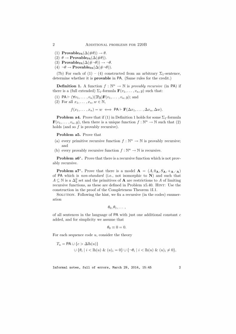
2 Additional problems for 220B
(1) ProvablePA(∆(#θ)) → θ.(2) θ → ProvablePA(∆(#θ)).(3) ProvablePA(∆(#¬θ)) → ¬θ.(4) ¬θ → ProvablePA(∆(#¬θ)).
(7b) For each of (1) – (4) constructed from an arbitrary Σ1-sentence,determine whether it is provable in PA. (Same rules for the credit.)
Definition 1. A function f : Nn → N is provably recursive (in PA) ifthere is a (full extended) Σ1-formula F(v1, . . . , vn, y) such that:
(1) PA ` (∀v1, . . . , vn)(∃!y)F(v1, . . . , vn, y); and(2) For all x1, . . . , xn, w ∈ N,
f(x1, . . . , xn) = w ⇐⇒ PA ` F(∆x1, . . . , ∆xn, ∆w).
Problem a4. Prove that if (1) in Definition 1 holds for some Σ1-formulaF(v1, . . . , vn, y), then there is a unique function f : Nn → N such that (2)holds (and so f is provably recursive).
Problem a5. Prove that
(a) every primitive recursive function f : Nn → N is provably recursive;and
(b) every provably recursive function f : Nn → N is recursive.
Problem a6∗. Prove that there is a recursive function which is not prov-ably recursive.
Problem a7∗. Prove that there is a model A = (A, 0A, SA, +A, ·A)of PA which is non-standard (i.e., not isomorphic to N) and such thatA ⊆ N is a ∆0
2 set and the primitives of A are restrictions to A of limitingrecursive functions, as these are defined in Problem x5.40. Hint: Use theconstruction in the proof of the Completeness Theorem 1I.1.
Solution. Following the hint, we fix a recursive (in the codes) enumer-ation
θ0, θ1, . . . ,
of all sentences in the language of PA with just one additional constant cadded, and for simplicity we assume that
θ0 ≡ 0 = 0.
For each sequence code u, consider the theory
Tu = PA ∪ c > ∆lh(u)∪ θi | i < lh(u) & (u)i = 0 ∪ ¬θi | i < lh(u) & (u)i 6= 0,
Informal notes, full of errors, March 29, 2014, 15:45 2

Additional problems for 220B 3
and define a function f : N→ N by the following “complete recursion”:
f(0) = 0,
f(n + 1) =
0, if the theory Tu with u = 〈f(0), . . . , f(n)〉 is consistent,1, otherwise.
The usual argument for the Completeness Theorem shows that the set
T = θn | f(n) = 0is a consistent and complete extension of PA which then defines a modelof PA that is non-standard. So it is enough to prove that the graph of r isΣ0
2: because
θn ∈ T ⇐⇒ f(n) = 0, θ /∈ T ⇐⇒ f(n) = 1,
which shows that T is ∆02, and then all the primitives of the Henkin model
are defined from T and so have ∆02 graphs.
To show that the graph of f is Σ02 we use the Dedekind analysis:
f(n) = w ⇐⇒ (∃u)[Seq(u) & lh(u) = (n + 1) & (∀i ≤ n)[(u)i ≤ 1]
& (u)0 = 0 & (∀i < n)((u)i+1 = 0 ⇐⇒ Au ¹ i is consistent
)
& (u)n = w].
This is easily checked to be Σ02, once we check that the relation
P (u) ⇐⇒ Au is consistent
is Π01, which is routine.
Problem a8. Let φe : N N be the recursive partial function withcode e and let F be the set of codes of total recursive functions,
F = e | (∀n)[φe(n)↓ ].(1) Prove that there is a least set A ⊆ N such that
1 ∈ A, (∀e)([e ∈ F & (∀n)[φe(n) ∈ A]] =⇒ 2e ∈ A
).
(2) Prove that for this set A,
2e ∈ A =⇒ e ∈ F & (∀n)[φe(n) ∈ A].
(3) Define for each a ∈ A a total, recursive function fa : N → N so thatthe following conditions hold:
1. For all x, f1(x) = x + 1.2. If a = 2e ∈ A, then for all n and all but finitely many x,
fφe(n)(x) < fa(x).
Informal notes, full of errors, March 29, 2014, 15:45 3

![Logic Programming [10pt] Theory Lecture 2: [3pt] (In ... · Logic Programming Theory Lecture 2: (In)completeness for Propositional Prolog Alex Simpson School of Informatics 1st October](https://img.pdfslide.us/doc/110x75/5cc593ff88c993f0248dc550/logic-programming-10pt-theory-lecture-2-3pt-in-logic-programming-theory.jpg)


![PROVABILITY LOGIC - Sergei N. Artemov...intuitionistic propositional logic IPC in this logic. G¨odel’s provability cal- ... [Smiley, 1963] the axioms of GL appeared for the first](https://img.pdfslide.us/doc/110x75/5ea1a25033249d64601edea0/provability-logic-sergei-n-artemov-intuitionistic-propositional-logic-ipc.jpg)
![Completeness of Propositional Logic as a Programryan/papers/complete.pdf · as the completeness theorem for propositional logic. In his doctoral dissertation of 1920 Post [13] was](https://img.pdfslide.us/doc/110x75/5f527e369876197cc04a77e3/completeness-of-propositional-logic-as-a-program-ryanpapers-as-the-completeness.jpg)