Embed Size (px)
Citation preview

Copyright © by SIAM. Unauthorized reproduction of this article is prohibited.
SIAM J. MATRIX ANAL. APPL. c© 2008 Society for Industrial and Applied MathematicsVol. 30, No. 2, pp. 609–638
H2 MODEL REDUCTION FOR LARGE-SCALE LINEARDYNAMICAL SYSTEMS∗
S. GUGERCIN† , A. C. ANTOULAS‡ , AND C. BEATTIE†
Abstract. The optimal H2 model reduction problem is of great importance in the area of dy-namical systems and simulation. In the literature, two independent frameworks have evolved focusingeither on solution of Lyapunov equations on the one hand or interpolation of transfer functions on theother, without any apparent connection between the two approaches. In this paper, we develop a newunifying framework for the optimal H2 approximation problem using best approximation propertiesin the underlying Hilbert space. This new framework leads to a new set of local optimality condi-tions taking the form of a structured orthogonality condition. We show that the existing Lyapunov-and interpolation-based conditions are each equivalent to our conditions and so are equivalent toeach other. Also, we provide a new elementary proof of the interpolation-based condition that clar-ifies the importance of the mirror images of the reduced system poles. Based on the interpolationframework, we describe an iteratively corrected rational Krylov algorithm for H2 model reduction.The formulation is based on finding a reduced order model that satisfies interpolation-based first-order necessary conditions for H2 optimality and results in a method that is numerically effectiveand suited for large-scale problems. We illustrate the performance of the method with a variety ofnumerical experiments and comparisons with existing methods.
Key words. model reduction, rational Krylov, H2 approximation
AMS subject classifications. 34C20, 41A05, 49K15, 49M05, 93A15, 93C05, 93C15
DOI. 10.1137/060666123
1. Introduction. Given a dynamical system described by a set of first-orderdifferential equations, the model reduction problem seeks to replace this original setof equations with a (much) smaller set of such equations so that the behavior of bothsystems is similar in an appropriately defined sense. Such situations arise frequentlywhen physical systems need to be simulated or controlled; the greater the level of detailthat is required, the greater the number of resulting equations. In large-scale settings,computations become infeasible due to limitations on computational resources as wellas growing inaccuracy due to numerical ill-conditioning. In all these cases the numberof equations involved may range from a few hundred to a few million. Examplesof large-scale systems abound, ranging from the design of VLSI (very large scaleintegration) chips to the simulation and control of MEMS (microelectromechanicalsystem) devices. For an overview of model reduction for large-scale dynamical systemswe refer to the book [2]. See also [23] for a recent collection of large-scale benchmarkproblems.
In this paper, we consider single input/single output (SISO) linear dynamicalsystems represented as
(1.1) G :
{x(t) = Ax(t) + bu(t)y(t) = cTx(t)
or G(s) = cT (sI − A)−1b,
∗Received by the editors July 26, 2006; accepted for publication (in revised form) by P. BennerFebruary 25, 2008; published electronically June 6, 2008.
http://www.siam.org/journals/simax/30-2/66612.html†Department of Mathematics, Virginia Tech, Blacksburg, VA ([email protected], [email protected]).
The work of these authors was supported in part by the NSF through grants DMS-050597 andDMS-0513542, and by the AFOSR through grant FA9550-05-1-0449.
‡Department of Electrical and Computer Engineering, Rice University, Houston, TX ([email protected]). The work of this author was supported in part by the NSF through grants CCR-0306503and ACI-0325081.
609
Dow
nloa
ded
07/0
1/12
to 1
98.8
2.17
7.50
. Red
istr
ibut
ion
subj
ect t
o SI
AM
lice
nse
or c
opyr
ight
; see
http
://w
ww
.sia
m.o
rg/jo
urna
ls/o
jsa.
php

Copyright © by SIAM. Unauthorized reproduction of this article is prohibited.
610 S. GUGERCIN, A. C. ANTOULAS, AND C. BEATTIE
where A ∈ Rn×n, b, c ∈ R
n; we define x(t) ∈ Rn, u(t) ∈ R, y(t) ∈ R as the state,
input, and output, respectively, of the system. (We comment on extensions to themultiple input/multiple output (MIMO) case in section 3.2.1, but will confine ouranalysis and examples to the SISO case.)
G(s) is the transfer function of the system: if u(s) and y(s) denote the Laplacetransforms of the input and output u(t) and y(t), respectively, then y(s) = G(s)u(s).With a standard abuse of notation, we will denote both the system and its transferfunction by G. The “dimension of G” is taken to be the dimension of the underlyingstate space, dimG = n in this case. It will always be assumed that the system, G, isstable, that is, that the eigenvalues of A have strictly negative real parts.
The model reduction process will yield another system,
(1.2) Gr :
{xr(t) = Arxr(t) + bru(t)yr(t) = cTr xr(t)
or Gr(s) = cTr (sI − Ar)−1br,
having (much) smaller dimension r � n, with Ar ∈ Rr×r and br, cr ∈ R
r.We want yr(t) ≈ y(t) over a large class of inputs u(t). Different measures of ap-
proximation and different choices of input classes will lead to different model reductiongoals. Suppose one wants to ensure that maxt>0 |y(t)− yr(t)| is small uniformly overall inputs, u(t), having bounded “energy,” that is,
∫∞0
|u(t)|2 dt ≤ 1. Observe firstthat y(s) − yr(s) = [G(s) −Gr(s)] u(s) and then
maxt>0
|y(t) − yr(t)| = maxt>0
∣∣∣∣ 1
2π
∫ ∞
−∞(y(ıω) − yr(ıω)) eıωt dω
∣∣∣∣≤ 1
2π
∫ ∞
−∞|y(ıω) − yr(ıω)| dω =
1
2π
∫ ∞
−∞|G(ıω) −Gr(ıω)| |u(ıω)| dω
≤(
1
2π
∫ ∞
−∞|G(ıω) −Gr(ıω)|2 dω
)1/2 (1
2π
∫ ∞
−∞|u(ıω)|2 dω
)1/2
≤(
1
2π
∫ ∞
−∞|G(ıω) −Gr(ıω)|2 dω
)1/2 (∫ ∞
0
|u(t)|2 dt
)1/2
≤(
1
2π
∫ +∞
−∞|G(ıω) −Gr(ıω)|2 dω
)1/2def= ‖G−Gr‖H2
.
We seek a reduced order dynamical system, Gr, such that(i) ‖G−Gr‖H2 , the “H2 error,” is as small as possible;(ii) critical system properties for G (such as stability) exist also in Gr; and(iii) the computation of Gr (i.e., the computation of Ar, br, and cr) is both
efficient and numerically stable.The problem of finding reduced order models that yield a small H2 error has
been the object of many investigations; see, for instance, [6, 37, 34, 9, 21, 26, 22, 36,25, 13] and the references therein. Finding a global minimizer of ‖G − Gr‖H2 is ahard task, so the goal in making ‖G −Gr‖H2 “as small as possible” becomes, as formany optimization problems, identification of reduced order models, Gr, that satisfyfirst-order necessary conditions for local optimality. There is a wide variety of suchconditions that may be derived, yet their interconnections are generally unclear. Mostmethods that can identify reduced order models satisfying such first-order necessaryconditions will require dense matrix operations, typically the solution of a sequenceof matrix Lyapunov equations, a task which becomes computationally intractable
Dow
nloa
ded
07/0
1/12
to 1
98.8
2.17
7.50
. Red
istr
ibut
ion
subj
ect t
o SI
AM
lice
nse
or c
opyr
ight
; see
http
://w
ww
.sia
m.o
rg/jo
urna
ls/o
jsa.
php

Copyright © by SIAM. Unauthorized reproduction of this article is prohibited.
H2 MODEL REDUCTION 611
rapidly as the dimension increases. Such methods are unsuitable even for medium-scale problems. In section 2, we review the moment matching problem for modelreduction, its connection with rational Krylov methods (which are very useful forlarge-scale problems), and basic features of the H2 norm and inner product.
We offer in section 3 what appears to be a new set of first-order necessary condi-tions for local optimality of a reduced order model comprising in effect a structuredorthogonality condition. We also show its equivalence with two other H2 optimalityconditions that have been previously known (thus showing them all to be equivalent).
An iterative algorithm that is designed to force optimality with respect to a set ofconditions that is computationally tractable is described in section 4. The proposedmethod also forces optimality with respect to the other equivalent conditions as well.It is based on computationally effective use of rational Krylov subspaces and so issuitable for systems whose dimension n is of the order of many thousands of statevariables. Numerical examples are presented in section 5.
2. Background.
2.1. Model reduction by moment matching. Given the system (1.1), reduc-tion by moment matching consists in finding a system (1.2) so that Gr(s) interpolatesthe values of G(s), and perhaps also derivative values as well, at selected interpolationpoints (also called shifts) σk in the complex plane. For our purposes, simple Hermiteinterpolation suffices, so our problem is to find Ar, br, and cr so that
Gr(σk) = G(σk) and G′r(σk) = G′(σk) for k = 1, . . . , r
or, equivalently,
cT (σkI − A)−1b = cTr (σkI − Ar)−1br and cT (σkI − A)−2b = cTr (σkI − Ar)
−2br
for k = 1, . . . , r. The quantity cT (σkI − A)−(j+1)b is called the jth moment ofG(s) at σk. Moment matching for finite σ ∈ C becomes rational interpolation; see, forexample, [3]. Importantly, these problems can be solved in a recursive and numericallyeffective way by means of rational Lanczos/Arnoldi procedures.
To see this we first consider reduced order models that are constructed by Galerkinapproximation: Let Vr and Wr be given r-dimensional subspaces of R
n that aregeneric in the sense that Vr ∩W⊥
r = {0}. Then for any input u(t) the reduced orderoutput yr(t) is defined by
Find v(t) ∈ Vr such that v(t)−Av(t) − bu(t) ⊥ Wr for all t;(2.1)
then yr(t)def= cTv(t).
Denote by Ran(M) the range of a matrix M. Let Vr ∈ Rn×r and Wr ∈ R
n×r bematrices defined so that Vr = Ran(Vr) and Wr = Ran(Wr). Then the assumptionVr∩W⊥
r = {0} is equivalent to WTr Vr being nonsingular. The Galerkin approximation
(2.1) can be interpreted as v(t) = Vrxr(t) with xr(t) ∈ Rr for each t and
WTr (Vrxr(t) − AVrxr(t) − bu(t)) = 0
leading then to the reduced order model (1.2) with
Ar = (WTr Vr)
−1WTr AVr, br = (WT
r Vr)−1WT
r b, and cTr = cTVr.(2.2)
Evidently the choice of Vr and Wr determines the quality of the reduced order model.
Dow
nloa
ded
07/0
1/12
to 1
98.8
2.17
7.50
. Red
istr
ibut
ion
subj
ect t
o SI
AM
lice
nse
or c
opyr
ight
; see
http
://w
ww
.sia
m.o
rg/jo
urna
ls/o
jsa.
php

Copyright © by SIAM. Unauthorized reproduction of this article is prohibited.
612 S. GUGERCIN, A. C. ANTOULAS, AND C. BEATTIE
Rational interpolation by projection was first proposed by Skelton et al. in [11, 38,39]. Grimme [17] showed how one can obtain the required projection using the rationalKrylov method of Ruhe [33]. Krylov-based methods are able to match momentswithout ever computing them explicitly. This is important since the computation ofmoments is in general ill-conditioned. This is a fundamental motivation behind theKrylov-based methods [12].
In Lemma 2.1 and Corollary 2.2 below, we present new short proofs of rationalinterpolation by Krylov projection that are substantially simpler than those found inthe original works [17, 11, 38, 39].
Lemma 2.1. Suppose σ ∈ C is not an eigenvalue of either A or Ar.
If (σI − A)−1b ∈ Vr, then Gr(σ) = G(σ).(2.3)
If (σ I − AT )−1c ∈ Wr, then Gr(σ) = G(σ).(2.4)
If both (σI − A)−1b ∈ Vr and (σ I − AT )−1c ∈ Wr,
then Gr(σ) = G(σ) and G′r(σ) = G′(σ).(2.5)
Proof. Define Nr(z) = Vr(zI − Ar)−1(WT
r Vr)−1WT
r (zI − A) and Nr(z) =
(zI−A)Nr(z)(zI−A)−1. Both Nr(z) and Nr(z) are analytic matrix-valued functionsin a neighborhood of z = σ. One may directly verify that N2
r(z) = Nr(z) and
N2r(z) = Nr(z) and that Vr = Ran Nr(z) = Ker (I − Nr(z)) and W⊥
r = Ker Nr(z) =
Ran(I − Nr(z)
)for all z in a neighborhood of σ. Then
G(z) −Gr(z) =[(zI − AT )−1c
]T (I − Nr(z)
)(zI − A)
(I − Nr(z)
)(zI − A)−1b.
Evaluating at z = σ leads to (2.3) and (2.4). Evaluating at z = σ + ε and observingthat (σI + εI − A)−1 = (σI − A)−1 − ε(σI − A)−2 + O(ε2) yields
G(σ + ε) −Gr(σ + ε) = O(ε2),
which gives (2.5) as a consequence.Corollary 2.2. Consider the system G defined by A,b, c, a set of distinct shifts
given by {σk}rk=1, that is closed under conjugation (i.e., shifts are either real or occurin conjugate pairs), and subspaces spanned by the columns of Vr and Wr with
Ran(Vr) = span{(σ1I − A)−1b, . . . , (σrI − A)−1b
}and(2.6)
Ran(Wr) = span{(σ1I − AT )−1c, . . . , (σrI − AT )−1c
}.(2.7)
Then Vr and Wr can be chosen to be real matrices and the reduced order system Gr
defined by Ar = (WTr Vr)
−1WTr AVr, br = (WT
r Vr)−1WT
r b, cTr = cTVr is itself realand matches the first two moments of G(s) at each of the interpolation points σk, i.e.,G(σk) = Gr(σk) and G′(σk) = G′
r(σk) for k = 1, . . . , r.For Krylov-based model reduction, one chooses interpolation points and then con-
structs Vr and Wr satisfying (2.6) and (2.7), respectively. Note that, in a numericalimplementation, one does not actually compute (σiI − A)−1, but instead computesa (potentially sparse) factorization (one for each interpolation point σi), uses it tosolve a system of equations having b as a right-hand side, and uses its transpose tosolve a system of equations having c as a right-hand side. The interpolation pointsare chosen so as to minimize the deviation of Gr from G in a sense that is detailed inthe next section. Unlike Gramian-based model reduction methods such as balancedtruncation (see section 2.2 below and [2]), Krylov-based model reduction requires only
Dow
nloa
ded
07/0
1/12
to 1
98.8
2.17
7.50
. Red
istr
ibut
ion
subj
ect t
o SI
AM
lice
nse
or c
opyr
ight
; see
http
://w
ww
.sia
m.o
rg/jo
urna
ls/o
jsa.
php

Copyright © by SIAM. Unauthorized reproduction of this article is prohibited.
H2 MODEL REDUCTION 613
matrix-vector multiplications and some sparse linear solvers, and can be iterativelyimplemented; hence it is computationally effective; for details, see also [15, 16].
2.2. Model reduction by balanced truncation. One of the most commonmodel reduction techniques is balanced truncation [28, 27]. In this case, the modelingsubspaces Vr and Wr depend on the solutions to the two Lyapunov equations
AP + PAT + bbT = 0, ATQ + QA + cT c = 0.(2.8)
P and Q are called the reachability and observability Gramians, respectively. Underthe assumption that A is stable, both P and Q are positive semidefinite matrices.Square roots of the eigenvalues of the product PQ are the singular values of theHankel operator associated with G(s) and are called the Hankel singular values ofG(s), denoted by ηi(G).
Let P = UUT and Q = LLT . Let UTL = ZSYT be the singular value decompo-sition with S = diag(η1, η2, . . . , ηn). Let Sr = diag(η1, η2, . . . , ηr), r < n. Construct
Wr = LYrS−1/2r and Vr = UZrS
−1/2r ,(2.9)
where Zr and Yr denote the leading r columns of left singular vectors, Z, and rightsingular vectors, Y, respectively. The rth-order reduced order model via balancedtruncation, Gr(s), is obtained by reducing G(s) using Wr and Vr from (2.9).
Another important dynamical systems norm (besides the H2 norm) is the H∞norm defined as ‖G‖H∞
:= supω∈R|G(ıω)|. The reduced order system Gr(s) obtained
by balanced truncation is asymptotically stable and the H∞ norm of the error systemsatisfies ‖G−Gr‖H∞
≤ 2(ηr+1 + · · · + ηn).The value of having, for reduced order models, guaranteed stability and an explicit
error bound is widely recognized, though it is achieved at potentially considerablecost. As described above, balanced truncation requires the solution of two Lyapunovequations of order n, which is a formidable task in large-scale settings. For moredetails and background on balanced truncation, see section III.7 of [2].
2.3. The H2 norm. H2 will denote the set of functions, g(z), that are analyticfor z in the open right half plane, Re(z) > 0, and such that for each fixed Re(z) =x > 0, g(x+ ıy) is square integrable as a function of y ∈ (−∞,∞) in such a way that
supx>0
∫ ∞
−∞|g(x + ıy)|2 dy < ∞.
H2 is a Hilbert space and holds our interest because transfer functions associated withstable SISO finite-dimensional dynamical systems are elements of H2. Indeed, if G(s)and H(s) are transfer functions associated with real stable SISO dynamical systems,then the H2 inner product can be defined as
(2.10) 〈G, H〉H2
def=
1
2π
∫ ∞
−∞G(ıω)H(ıω) dω =
1
2π
∫ ∞
−∞G(−ıω)H(ıω) dω,
with a norm defined as
(2.11) ‖G‖H2
def=
(1
2π
∫ +∞
−∞|G(ıω)|2 dω
)1/2
.
Notice in particular that if G(s) and H(s) represent real dynamical systems, then〈G, H〉H2 = 〈H, G〉H2 and 〈G, H〉H2 must be real.
Dow
nloa
ded
07/0
1/12
to 1
98.8
2.17
7.50
. Red
istr
ibut
ion
subj
ect t
o SI
AM
lice
nse
or c
opyr
ight
; see
http
://w
ww
.sia
m.o
rg/jo
urna
ls/o
jsa.
php

Copyright © by SIAM. Unauthorized reproduction of this article is prohibited.
614 S. GUGERCIN, A. C. ANTOULAS, AND C. BEATTIE
There are two alternate characterizations of this inner product that make it farmore computationally accessible.
Lemma 2.3. Suppose A ∈ Rn×n and B ∈ R
m×m are stable and, given b, c ∈ Rn
and b, c ∈ Rm, define associated transfer functions,
G(s) = cT (sI − A)−1
b and H(s) = cT (sI − B)−1
b.
The inner product 〈G, H〉H2is associated with solutions to Sylvester equations as
follows:
If P solves AP + PBT + bbT = 0, then 〈G, H〉H2= cTPc.(2.12)
If Q solves QA + BTQ + ccT = 0, then 〈G, H〉H2= bTQb.(2.13)
If R solves AR + RB + bcT = 0, then 〈G, H〉H2= cTRb.(2.14)
Note that if A = B, b = b, and c = c, then P is the “reachability Gramian” of G(s),Q is the “observability Gramian” of G(s), and R is the “cross Gramian” of G(s); and
(2.15) ‖G‖2H2
= cTPc = bTQb = cTRb.
Gramians play a prominent role in the analysis of linear dynamical systems; referto [2] for more information.
Proof. We detail the proof of (2.12); proofs of (2.13) and (2.14) are similar. SinceA and B are stable, the solution, P, to the Sylvester equation of (2.12) exists and isunique. For any ω ∈ R, rearrange this equation to obtain in sequence
(−ıωI − A)P + P(ıωI − BT
)− bbT = 0,
(−ıωI − A)−1
P + P(ıωI − BT
)−1= (−ıωI − A)
−1bbT
(ıωI − BT
)−1,
cT (−ıωI − A)−1
Pc + cTP(ıωI − BT
)−1c = G(−ıω)H(ıω),
and finally
cT
(∫ L
−L
(−ıωI − A)−1
dω
)Pc + cTP
(∫ L
−L
(ıωI − BT
)−1dω
)c
=
∫ L
−L
G(−ıω)H(ıω) dω.
Taking L → ∞ and using Lemma A.1 in the appendix leads to∫ ∞
−∞G(−ıω)H(ıω) dω = cT
(P.V.
∫ ∞
−∞(−ıωI − A)
−1dω
)Pc
+ cTP
(P.V.
∫ ∞
−∞
(ıωI − BT
)−1dω
)c
= 2π cTPc.
Recently, Antoulas [2] obtained a new expression for ‖G‖H2 based on the polesand residues of the transfer function G(s) that complements the widely known alter-native expression (2.15). We provide a compact derivation of this expression and theassociated H2 inner product.
Dow
nloa
ded
07/0
1/12
to 1
98.8
2.17
7.50
. Red
istr
ibut
ion
subj
ect t
o SI
AM
lice
nse
or c
opyr
ight
; see
http
://w
ww
.sia
m.o
rg/jo
urna
ls/o
jsa.
php

Copyright © by SIAM. Unauthorized reproduction of this article is prohibited.
H2 MODEL REDUCTION 615
If f(s) is a meromorphic function with a pole at λ, denote the residue of f(s) at λby res[f(s), λ]. Thus, if λ is a simple pole of f(s), then res[f(s), λ] = lims→λ(s−λ)f(s),and if λ is a double pole of f(s), then res[f(s), λ] = lims→λ
dds
[(s− λ)2f(s)
].
Lemma 2.4. Suppose that G(s) has poles at λ1, λ2, . . . , λn and H(s) has poles atμ1, μ2, . . . , μm, both sets contained in the open left half plane. Then
(2.16) 〈G, H〉H2=
m∑k=1
res[G(−s)H(s), μk] =
n∑k=1
res[H(−s)G(s), λk].
In particular,• if μk is a simple pole of H(s), then
res[G(−s)H(s), μk] = G(−μk)res[H(s), μk];
• if μk is a double pole of H(s), then
res[G(−s)H(s), μk] = G(−μk) res[H(s), μk] −G′(−μk) · h0(μk),
where h0(μk) = lims→μk
((s− μk)
2H(s)).
Proof. Notice that the function G(−s)H(s) has singularities at μ1, μ2, . . . , μm
and −λ1, −λ2, . . . ,−λn. For any R > 0, define the semicircular contour in the lefthalf plane:
ΓR = {z |z = ıω with ω ∈ [−R,R]} ∪{z
∣∣∣∣z = Reıθ with θ ∈[π
2,3π
2
]}.
ΓR bounds a region that for sufficiently large R contains all the system poles of H(s)and so, by the residue theorem,
〈G, H〉H2=
1
2π
∫ +∞
−∞G(−ıω)H(ıω) dω
= limR→∞
1
2πı
∫ΓR
G(−s)H(s) ds =
m∑k=1
res[G(−s)H(s), μk].
Evidently, if μk is a simple pole for H(s), it is also a simple pole for G(−s)H(s) and
res[G(−s)H(s), μk] = lims→μk
(s− μk)G(−s)H(s) = G(−μk) lims→μk
(s− μk)H(s).
If μk is a double pole for H(s), then it is also a double pole for G(−s)H(s) and
res[G(−s)H(s), μk] = lims→μk
d
ds(s− μk)
2G(−s)H(s)
= lims→μk
G(−s)d
ds(s− μk)
2H(s) −G′(−s)(s− μk)2H(s)
= G(−μk) lims→μk
d
ds(s− μk)
2H(s) −G′(−μk) lims→μk
(s− μk)2H(s).
Lemma 2.4 immediately yields the expression for ‖G‖H2 given by Antoulas [2,p. 145] based on poles and residues of the transfer function G(s).
Corollary 2.5. If G(s) has simple poles at λ1, λ2, . . . , λn, then
‖G‖H2=
(n∑
k=1
res[G(s), λk]G(−λk)
)1/2
.
Dow
nloa
ded
07/0
1/12
to 1
98.8
2.17
7.50
. Red
istr
ibut
ion
subj
ect t
o SI
AM
lice
nse
or c
opyr
ight
; see
http
://w
ww
.sia
m.o
rg/jo
urna
ls/o
jsa.
php
Copyright © by SIAM. Unauthorized reproduction of this article is prohibited.
616 S. GUGERCIN, A. C. ANTOULAS, AND C. BEATTIE
3. Optimal H2 model reduction. In this section, we investigate three frame-works of necessary conditions for H2 optimality. The first utilizes the inner productstructure H2 and leads to what could be thought of as a geometric condition for opti-mality. This appears to be a new characterization of H2 optimality for reduced ordermodels. The remaining two frameworks, interpolation-based [26] and Lyapunov-based[36, 22], are easily derived from the first framework and in this way can be seen to beequivalent to one another—a fact that is not a priori evident. This equivalence provesthat solving the optimal H2 problem in the Krylov framework is equivalent to solvingit in the Lyapunov framework, which leads to the proposed Krylov-based method forH2 model reduction in section 4.
Given G, a stable SISO finite-dimensional dynamical system as described in (1.1),we seek a stable reduced order system Gr of order r as described in (1.2), which isthe best stable rth-order dynamical system approximating G with respect to the H2
norm:
(3.1) ‖G−Gr‖H2 = mindim(Gr)=r
Gr : stable
‖G− Gr‖H2 .
Many researchers have worked on problem (3.1), the optimal H2 model reductionproblem. See [37, 34, 9, 21, 26, 22, 36, 25] and the references therein.
3.1. Structured orthogonality optimality conditions. The set of all stablerth-order dynamical systems do not constitute a subspace of H2, so the best rth-order H2 approximation is not so easy to characterize, the Hilbert space structureof H2 notwithstanding. This observation does suggest the following narrower thoughsimpler result.
Theorem 3.1. Let μ1, μ2, . . . , μr ⊂ C be distinct points in the open left halfplane and define M(μ) to be the set of all proper rational functions that have simplepoles exactly at μ1, μ2, . . . , μr. Then
• H ∈ M(μ) implies that H is the transfer function of a stable dynamicalsystem with dim(H) = r;
• M(μ) is an (r − 1)-dimensional subspace of H2;• Gr ∈ M(μ) solves
(3.2) ‖G−Gr‖H2 = minGr∈M(μ)
‖G− Gr‖H2
if and only if
(3.3) 〈G−Gr, H〉H2= 0 for all H ∈ M(μ).
Furthermore the solution, Gr, to (3.2) exists and is unique.Proof. The key observation is that M(μ) is a closed subspace of H2. Then the
equivalence of (3.2) and (3.3) follows from the classic projection theorem in Hilbertspace (cf. [32]).
One consequence of Theorem 3.1 is that if Gr(s) interpolates a real system G(s)at the mirror images of its own poles (i.e., at the poles of Gr(s) reflected acrossthe imaginary axis), then Gr(s) is guaranteed to be an optimal approximation ofG(s) relative to the H2 norm among all reduced order systems having the samereduced system poles {μi}ri=1. An analogous result for optimal rational approximantsto analytic functions on the unit disk can be found in [14]. The set of stable rth-order dynamical systems is not convex, and so the original problem (3.1) allows for
Dow
nloa
ded
07/0
1/12
to 1
98.8
2.17
7.50
. Red
istr
ibut
ion
subj
ect t
o SI
AM
lice
nse
or c
opyr
ight
; see
http
://w
ww
.sia
m.o
rg/jo
urna
ls/o
jsa.
php

Copyright © by SIAM. Unauthorized reproduction of this article is prohibited.
H2 MODEL REDUCTION 617
multiple minimizers. Indeed there may be “local minimizers” that do not solve (3.1).A reduced order system, Gr, is a local minimizer for (3.1) if, for all ε > 0 sufficientlysmall,
(3.4) ‖G−Gr‖H2 ≤ ‖G− G(ε)r ‖H2
for all stable dynamical systems G(ε)r with dim(G
(ε)r ) = r and ‖Gr − G
(ε)r ‖H2 ≤ C ε,
with C being a constant that may depend on the particular family G(ε)r considered.
As a practical matter, the global minimizers that solve (3.1) are difficult to obtainwith certainty; current approaches favor seeking reduced order models that satisfy alocal (first-order) necessary condition for optimality. Even though such strategies donot guarantee global minimizers, they often produce effective reduced order modelsnonetheless. In this spirit, we give necessary conditions for optimality for the reducedorder system, Gr, that appear as structured orthogonality conditions similar to (3.3).
Theorem 3.2. If Gr is a local minimizer to G as described in (3.4) and Gr hassimple poles, then
(3.5) 〈G−Gr, Gr ·H1 + H2〉H2= 0
for all real dynamical systems H1 and H2 having the same poles with the same mul-tiplicities as Gr.
(Gr ·H1 here denotes pointwise multiplication of scalar functions.)Proof. Theorem 3.1 implies (3.5) with H1 = 0, so it suffices to show that the
hypotheses imply that 〈G−Gr, Gr ·H〉H2= 0 for all real dynamical systems H
having the same poles with the same multiplicities as Gr.
Suppose that {G(ε)r }ε>0 is a family of real stable dynamical systems with
dim(G(ε)r ) = r and ‖Gr − G
(ε)r ‖H2 < Cε for some constant C > 0. Then for all
ε > 0 sufficiently small,
‖G−Gr‖2H2
≤ ‖G− G(ε)r ‖2
H2
≤ ‖(G−Gr) + (Gr − G(ε)r )‖2
H2
≤ ‖G−Gr‖2H2
+ 2⟨G−Gr, Gr − G(ε)
r
⟩H2
+ ‖Gr − G(ε)r )‖2
H2.
This in turn implies for all ε > 0 sufficiently small that
(3.6) 0 ≤ 2⟨G−Gr, Gr − G(ε)
r
⟩H2
+ ‖Gr − G(ε)r ‖2
H2.
By considering a few different “directions of approach” of G(ε)r to Gr as ε → 0,
(3.6) will lead to a few different necessary conditions for Gr to be a locally optimalreduced order model. Denote the poles of Gr as μ1, μ2, . . . , μr and suppose they areordered so that the first mR are real and the next mC are in the upper half plane.Write μi = αi + ıβi. Any real rational function having the same poles as Gr(s) canbe written as
H(s) =
mR∑i=1
γis− μi
+
mR+mC∑i=mR+1
ρi(s− αi) + τi(s− αi)2 + β2
i
,
with arbitrary real-valued choices for γi, ρi, and τi. Now suppose that μ is a real polefor Gr and that
(3.7)
⟨G−Gr,
Gr(s)
s− μ
⟩H2
�= 0.
Dow
nloa
ded
07/0
1/12
to 1
98.8
2.17
7.50
. Red
istr
ibut
ion
subj
ect t
o SI
AM
lice
nse
or c
opyr
ight
; see
http
://w
ww
.sia
m.o
rg/jo
urna
ls/o
jsa.
php

Copyright © by SIAM. Unauthorized reproduction of this article is prohibited.
618 S. GUGERCIN, A. C. ANTOULAS, AND C. BEATTIE
Write Gr(s) = pr−1(s)(s−μ) qr−1(s)
for real polynomials pr−1, qr−1 ∈ Pr−1 and define
G(ε)r (s) =
pr−1(s)
[s− μ− (±ε)] qr−1(s),
where the sign of ±ε is chosen to match that of⟨G−Gr,
Gr(s)s−μ
⟩H2
. Then we have
G(ε)r (s) = Gr(s) ± ε
pr−1(s)
(s− μ)2 qr−1(s)+ O(ε2),
which leads to Gr(s) − G(ε)r (s) = ∓εGr(s)
s−μ + O(ε2) and
(3.8)⟨G−Gr, Gr − G(ε)
r
⟩H2
= −ε
∣∣∣∣∣⟨G−Gr,
Gr(s)
s− μ
⟩H2
∣∣∣∣∣+ O(ε2).
Then (3.6) implies that as ε → 0, 0 <∣∣⟨G − Gr,
Gr(s)s−μ
⟩H2
∣∣ ≤ Cε for some constant
C, which then contradicts (3.7).Now suppose that μ = α + ıβ is a pole for Gr with a nontrivial imaginary part,
β �= 0, and so is one of a conjugate pair of poles for Gr. Suppose further that
(3.9)
⟨G−Gr,
Gr(s)
(s− α)2 + β2
⟩H2
�= 0 and
⟨G−Gr,
(s− α)Gr(s)
(s− α)2 + β2
⟩H2
�= 0.
Write Gr(s) = pr−1(s)[(s−α)2+β2] qr−2(s)
for some choice of real polynomials pr−1 ∈ Pr−1 and
qr−2 ∈ Pr−2. Arguments exactly analogous to the previous case lead to the remainingassertions. In particular,
to show
⟨G−Gr,
Gr(s)
(s− α)2 + β2
⟩H2
= 0,
consider G(ε)r (s) =
pr−1(s)
[(s− α)2 + β2 − (±ε)] qr−2(s);
to show
⟨G−Gr,
(s− α)Gr(s)
(s− α)2 + β2
⟩H2
= 0,
consider G(ε)r (s) =
pr−1(s)
[(s− α− (±ε))2
+ β2] qr−2(s).
The conclusion follows then by observing that if Gr is a locally optimal H2 reducedorder model, then
〈G−Gr, Gr ·H1 + H2〉H2 =
mR∑i=1
γi
⟨G−Gr,
Gr(s)
s− μi
⟩H2
+
mR+mC∑i=mR+1
ρi
⟨G−Gr,
(s− αi)Gr(s)
(s− αi)2 + β2i
⟩H2
+
mR+mC∑i=mR+1
τi
⟨G−Gr,
Gr(s)
(s− αi)2 + β2i
⟩H2
+ 〈G−Gr, H2(s)〉H2= 0.
Dow
nloa
ded
07/0
1/12
to 1
98.8
2.17
7.50
. Red
istr
ibut
ion
subj
ect t
o SI
AM
lice
nse
or c
opyr
ight
; see
http
://w
ww
.sia
m.o
rg/jo
urna
ls/o
jsa.
php

Copyright © by SIAM. Unauthorized reproduction of this article is prohibited.
H2 MODEL REDUCTION 619
Theorem 3.2 describes new necessary conditions for the H2 approximation prob-lem as structured orthogonality conditions. This new formulation amounts to a unify-ing framework for the optimal H2 problem. Indeed, as we show in sections 3.2 and 3.3,two other known optimality frameworks, namely, interpolatory- [26] and Lyapunov-based conditions [36, 22], can be directly obtained from our new conditions by usingan appropriate form for the H2 inner product. The interpolatory framework uses theresidue formulation of the H2 inner product as in (2.16); the Lyapunov frameworkuses the Sylvester equation formulation of the H2 norm as in (2.12).
3.2. Interpolation-based optimality conditions. Corollary 2.5 immediatelyyields an observation regarding the H2 norm of the error system, which serves as amain motivation for the interpolation framework of the optimal H2 problem.
Proposition 3.3. Given the full-order model G(s) and a reduced order model
Gr(s), let λi and λi be the poles of G(s) and Gr(s), respectively, and suppose that
the poles of Gr(s) are distinct. Let φi and φj denote the residues of the transfer
functions G(s) and Gr(s) at their poles λi and λi, respectively: φi = res[G(s), λi] for
i = 1, . . . , n and φj = res[Gr(s), λj ] for j = 1, . . . , r. The H2 norm of the error systemis given by
‖G−Gr‖2H2
=
n∑i=1
res[(G(−s) −Gr(−s)) (G(s) −Gr(s)) , λi]
+
r∑j=1
res[(G(−s) −Gr(−s)) (G(s) −Gr(s)) , λj ]
=
n∑i=1
φi
(G(−λi) −Gr(−λi)
)−
r∑j=1
φj
(G(−λj) −Gr(−λj)
).(3.10)
The H2 error expression (3.10) is valid for any reduced order model regardlessof the underlying reduction technique and generalizes a result of [20, 18] to the mostgeneral setting.
Proposition 3.3 has the system-theoretic interpretation that the H2 error is dueto mismatch of the transfer functions G(s) and Gr(s) at mirror images of the full-
order poles λi and reduced order poles λi. This expression reveals that for good H2
performance, Gr(s) should approximate G(s) well at −λi and −λj . Note that λi isnot known a priori. Therefore, to minimize the H2 error, Gugercin and Antoulas[20] proposed choosing σi = −λi(A), where λi(A) are those system poles having bigresiduals φi. They have illustrated that this selection of interpolation points worksquite well; see [18, 20]. However, as (3.10) illustrates, there is a second part of the H2
error due to the mismatch at −λj . Indeed, as we will show below, interpolation at
−λi is more important for model reduction and is a necessary condition for optimalH2 model reduction; i.e., σi = −λi is the optimal shift selection.
Theorem 3.4. Given a stable SISO system G(s) = cT (sI − A)−1b, let Gr(s) =cTr (sI−Ar)
−1br be a local minimizer of dimension r for the optimal H2 model reduc-
tion problem (3.1) and suppose that Gr(s) has simple poles at λi, i = 1, . . . , r. Then
Gr(s) interpolates both G(s) and its first derivative at −λi, i = 1, . . . , r:
Gr(−λi) = G(−λi) and G′r(−λi) = G′(−λi) for i = 1, . . . , r.(3.11)
Proof. From (3.5), consider first the case H1 = 0 and H2 is an arbitrary transfer
function with simple poles at λi, i = 1, . . . , r. Denote φi = res[H2(s), λi]. Then (2.16)
Dow
nloa
ded
07/0
1/12
to 1
98.8
2.17
7.50
. Red
istr
ibut
ion
subj
ect t
o SI
AM
lice
nse
or c
opyr
ight
; see
http
://w
ww
.sia
m.o
rg/jo
urna
ls/o
jsa.
php

Copyright © by SIAM. Unauthorized reproduction of this article is prohibited.
620 S. GUGERCIN, A. C. ANTOULAS, AND C. BEATTIE
leads to
〈G−Gr, H2〉H2=
r∑i=1
res[(G(−s) −Gr(−s))H2(s), λi]
=
r∑i=1
φi
(G(−λi) −Gr(−λi)
)= 0.
Since this is true for arbitrary choices of φi, we have G(−λi) = Gr(−λi). Nowconsider the case H2 = 0 and H1 is an arbitrary transfer function with simple polesat λi, i = 1, . . . , r. Then Gr(s)H1(s) has double poles at λi, i = 1, . . . , r, and since
G(−λi) = Gr(−λi) we have
〈G−Gr, Gr ·H1〉H2=
r∑i=1
res[(G(−s) −Gr(−s))Gr(s)H1(s), λi]
= −r∑
i=1
φi res[Gr, λi](G′(−λi) −G′
r(−λi))
= 0,
where we have calculated
lims→λi
((s− λi)
2Gr(s) ·H1(s))
= res[H1(s), λi] · res[Gr(s), λi] = φi res[Gr, λi].
We refer to the first-order conditions (3.11) as Meier–Luenberger conditions, rec-ognizing the work of [26], although we have here directly obtained them from thenewly derived structured orthogonality conditions (3.5).
In Theorem 3.4, we assume that the reduced order poles (eigenvalues of Ar) aresimple; analogous results for the case that Gr has a higher order pole are straightfor-ward and correspond to interpolation conditions of higher derivatives at the mirrorimages of reduced order poles.
3.2.1. Multiple input/multiple output systems. Many of these considera-tions extend naturally to the multiple input/multiple output (MIMO) setting:
(3.12) G :
{x(t) = Ax(t) + Bu(t)y(t) = Cx(t)
or G(s) = C(sI − A)−1B,
where the state vector x(t) ∈ Rn as before, but now the system has an input vector
u(t) ∈ Rm and output vector y(t) ∈ R
p, so that B ∈ Rn×m and C ∈ R
p×n forsome m, p ≥ 1. The transfer function, G(s), in (3.12) becomes matrix valued. Areduced order system analogous to (1.2) is sought with the same number of inputsm and outputs p, but with lower state space dimension r � n. If Vr ∈ R
n×r andWr ∈ R
n×r such that WTr Vr is nonsingular, we can define a (matrix-valued) reduced
order transfer function Gr(s) = Cr(sI − Ar)−1Br with
Ar = (WTr Vr)
−1WTr AVr, Br = (WT
r Vr)−1WT
r B, and Cr = CVr.
In order to assess “closeness” of MIMO systems, there is a natural extension ofthe Hilbert space, H2, to p ×m matrix-valued functions. In particular, if G(s) andH(s) are p × m matrix-valued transfer functions associated with real stable MIMOdynamical systems, then the associated H2 inner product is(3.13)
〈G, H〉H2
def=
1
2π
∫ ∞
−∞tr(G(ıω)HT (ıω)
)dω =
1
2π
∫ ∞
−∞tr(G(−ıω)HT (ıω)
)dω,
Dow
nloa
ded
07/0
1/12
to 1
98.8
2.17
7.50
. Red
istr
ibut
ion
subj
ect t
o SI
AM
lice
nse
or c
opyr
ight
; see
http
://w
ww
.sia
m.o
rg/jo
urna
ls/o
jsa.
php

Copyright © by SIAM. Unauthorized reproduction of this article is prohibited.
H2 MODEL REDUCTION 621
where “tr(M)” denotes the trace of the matrix M. The H2 norm is then
(3.14) ‖G‖H2
def=
(1
2π
∫ +∞
−∞‖G(ıω)‖2
F dω
)1/2
,
where ‖F‖Fdef=(∑
ij |Fij |2)1/2
denotes the usual Frobenius matrix norm. As before,if G(s) and H(s) represent real dynamical systems, then 〈G, H〉H2 = 〈H, G〉H2 and〈G, H〉H2 is real.
Necessary conditions for H2 optimality built on structured orthogonality parallel-ing the results of section 3.1 can be derived in this setting as well. In particular, theresidue form for the inner product is a straightforward analogue of Lemma 2.4 andleads naturally to interpolation conditions. If F(s) is a matrix-valued meromorphicfunction with a pole at λ, then F(s) has a Laurent expansion (with matrix coeffi-cients), and its residue, res[F(s), λ], will be the coefficient matrix associated with theexpansion term (s−λ)−1. For example, suppose that F(s) has the realization F(s) =
C(sI − A
)−1B. If λ is a simple pole of F(s), then we can assume that λ is a simple
eigenvalue of A associated with a rank-1 spectral projector Eλ and then F(s) =1
s−λEλ+D(s), where D(s) is analytic at s = λ, and res[F(s), λ] = lims→λ(s−λ)F(s) =
CEλB. If λ is a double pole, then we can assume that λ is a double eigenvalue ofA associated with a rank-2 spectral projector Eλ and a rank-1 nilpotent matrix Nλ
such that AEλ = λEλ + Nλ. Then F(s) = 1(s−λ)2 Nλ + 1
(s−λ)Eλ + D(s), where D(s)
is analytic at s = λ, and so res[F(s), λ] = lims→λdds
[(s− λ)2F(s)
]= CEλB.
Lemma 3.5. Suppose that G(s) has poles at λ1, λ2, . . . , λn and H(s) has poles
at λ1, λ2, . . . , λn, with both sets contained in the open left half plane. Then
(3.15) 〈G, H〉H2=
n∑k=1
tr(res[G(−s)HT (s), λk]
).
In particular, suppose H(s) has a realization H(s) = C(sI − A)−1B:
• If λk is a simple pole of H(s), and λk is associated with left and right eigen-
vectors of A, yk, and xk, respectively,
Axk = λk xk, y∗kA = λk y∗
k, and y∗kxk = 1,
thentr(res[G(−s)HT (s), λk]
)= cTk G(−λk)bk,
where bTk = y∗
kB and ck = Cxk.
• If λk is a double pole of H(s), and λk is associated with left and right eigen-
vectors yk and xk of A, and generalized eigenvectors, zk and wk, respectively,
Axk =λk xk, Awk = λk wk + xk, y∗kA = λk y∗
k, z∗kA = λk z∗k + y∗k,
and y∗kxk = 0, z∗kwk = 0, and z∗kxk = y∗
kwk = 1,
then
tr(res[G(−s)HT (s), λk]
)= dT
k G(−λk)bk + cTk G(−λk)ek − cTk G′(−λk)bk,
where bk and ck are as above and eTk = z∗kB and dk = Cwk.
Dow
nloa
ded
07/0
1/12
to 1
98.8
2.17
7.50
. Red
istr
ibut
ion
subj
ect t
o SI
AM
lice
nse
or c
opyr
ight
; see
http
://w
ww
.sia
m.o
rg/jo
urna
ls/o
jsa.
php

Copyright © by SIAM. Unauthorized reproduction of this article is prohibited.
622 S. GUGERCIN, A. C. ANTOULAS, AND C. BEATTIE
Now assume that Gr is an optimal reduced order model minimizing ‖G−Gr‖H2
in the sense described in (3.1) and suppose further that Gr has simple poles λi. Take
H(s) = Gr in (3.5) so that Gr(s) =∑
k1
s−λkckb
Tk and the residue of Gr(s) at λk is
matrix valued and rank one: res[Gr(s), λk] = ckbTk . An analysis paralleling what we
have carried out above yields analogous error expressions (see also [2]) and first-ordernecessary conditions for the MIMO optimal H2 reduction problem:
G(−λk)bk = Gr(−λk)bk,
cTk G(−λk) = cTk Gr(−λk), and(3.16)
cTk G′(−λk)bk = cTk G′r(−λk)bk, for k = 1, . . . , r.
The SISO (m = p = 1) conditions are replaced in the MIMO case by left tangential,right tangential, as well as bi-tangential interpolation conditions. From the discussionof section 2.1, if Ran(Vr) contains (λkI + A)−1Bbk and Ran(Wr) contains (λkI +A)−TCT ck for each k = 1, 2, . . . , r, then the H2 optimality conditions given abovehold. First-order interpolatory MIMO conditions have been obtained recently in otherindependent works as well; see [24, 35].
3.2.2. The discrete time case. An nth-order SISO discrete-time dynamicalsystem is defined by a set of difference equations
(3.17) G :
{x(t + 1) = Ax(t) + bu(t)
y(t) = cTx(t)or G(z) = cT (zI − A)−1b,
where t ∈ Z and A ∈ Rn×n, b, c ∈ R
n. G(z) is the transfer function of the system, sothat if u(z) and y(z) denote the z-transforms of u(t) and y(t), respectively, then y(z) =G(z)u(z). In this case, stability of G means that | λi(A) |< 1 for i = 1, . . . , n. Also,
the h2 norm is defined as ‖G‖2h2
= 12π
∫ 2π
0| G(eıθ) |2 dθ. Model reduction for discrete-
time systems is defined similarly. In this setting, interpolatory (necessary) conditionsfor h2 optimality of the rth-order reduced model Gr(z) = cTr (zI − Ar)
−1br become
G(1/λi
)= Gr
(1/λi
)and G′(1/λi
)= G′
r
(1/λi
)for i = 1, . . . , r, where λi denotes the
ith eigenvalue of Ar. This is a special case of results for discrete-time MIMO systemsformulated previously in [10].
3.3. Lyapunov-based H2 optimality conditions. In this section we brieflyreview the Lyapunov framework for the first-order H2 optimality conditions andpresent its connection to our structured orthogonality framework.
Given a stable SISO system G(s) = cT (sI−A)−1b, let Gr(s) = cTr (sI−Ar)−1br
be a local minimizer of dimension r for the optimal H2 model reduction problem (3.1)
and suppose that Gr(s) has simple poles at λi, i = 1, . . . , r.It is convenient to define the error system
Gerr(s)def= G(s) −Gr(s) = cTerr (sI − Aerr)
−1berr(3.18)
with Aerr =
[A 00 Ar
], berr =
[bbr
], and cTerr = [cT − cTr ].(3.19)
Let Perr and Qerr be the Gramians for the error system Gerr(s); i.e., Perr andQerr solve
AerrPerr + PerrATerr + berrb
Terr = 0,(3.20)
QerrAerr + ATerrQerr + cerrc
Terr = 0.(3.21)
Dow
nloa
ded
07/0
1/12
to 1
98.8
2.17
7.50
. Red
istr
ibut
ion
subj
ect t
o SI
AM
lice
nse
or c
opyr
ight
; see
http
://w
ww
.sia
m.o
rg/jo
urna
ls/o
jsa.
php

Copyright © by SIAM. Unauthorized reproduction of this article is prohibited.
H2 MODEL REDUCTION 623
Partition Perr and Qerr:
(3.22) Perr =
[P11 P12
PT12 P22
], Qerr =
[Q11 Q12
QT12 Q22
],
where P11,Q11 ∈ Rn×n and P22,Q22 ∈ R
r×r. Wilson [36] showed that the reducedorder model Gr(s) = cTr (sI−Ar)
−1br can be defined in terms of a Galerkin frameworkas well by taking
(3.23) Vr = P12P−122 and Wr = −Q12Q
−122 ,
and the resulting reduced order model satisfies the first-order conditions of the optimalH2 problem. It was also shown in [36] that WT
r Vr = I. The next result states theLyapunov-based Wilson conditions for H2 optimality and shows their equivalence toour structured orthogonality framework.
Theorem 3.6. The Wilson conditions for H2 optimality,
PT12Q12 + P22Q22 = 0,(3.24)
QT12b + Q22br = 0,(3.25)
cTr P22 − cTP12 = 0,(3.26)
are equivalent to the structured orthogonality conditions of Theorem 3.2.Proof. From (3.5), consider first the case H1 = 0 and H2 is an arbitrary transfer
function with simple poles at λi, i = 1, . . . , r. Write H2(s) = cT (sI−Ar)−1b, where
b and c can vary arbitrarily. Then from (2.12), if, for any b �= 0, [PT1 , P
T2 ]T solves
(3.27)
[A 00 Ar
][P1
P2
]+
[P1
P2
]AT
r +
[bbr
]bT = 0,
we have for arbitrary c
〈G−Gr, H2〉H2= [cT − cTr ]
[P1
P2
]c = 0.
Notice that P1 and P2 are independent of c, so for each choice of b we must have
cT P1 − cTr P2 = 0.
For b = br, one may check directly that P1 = P12 and P2 = P22 in Perr that solves(3.20) in Wilson’s conditions.
Likewise, from (2.13) for each choice of c, if [Q1, Q2] solves
(3.28) [Q1, Q2]
[A 00 Ar
]+ AT
r [Q1, Q2] + c[cT , −cTr ] = 0,
then we have for every b
〈G−Gr, H2〉H2= bT [Q1, Q2]
[bbr
]= 0.
Dow
nloa
ded
07/0
1/12
to 1
98.8
2.17
7.50
. Red
istr
ibut
ion
subj
ect t
o SI
AM
lice
nse
or c
opyr
ight
; see
http
://w
ww
.sia
m.o
rg/jo
urna
ls/o
jsa.
php

Copyright © by SIAM. Unauthorized reproduction of this article is prohibited.
624 S. GUGERCIN, A. C. ANTOULAS, AND C. BEATTIE
Similarly to the first case, [Q1, Q2] is independent of b, so for each choice of c wemust have
Q1b + Q2br = 0,
and for the particular case c = −cr, one may check directly that Q1 = QT12 and Q2 =
Q22 in Qerr that solves (3.21) in Wilson’s conditions. The structured orthogonalitycondition 〈G−Gr, H〉H2
= 0 taken over all systems H(s) with the same poles as Gr
leads directly to the Wilson conditions (3.25) and (3.26).The additional orthogonality condition 〈G−Gr, Gr ·H〉H2
= 0 taken over allH(s) with the same poles as Gr will yield the remaining Wilson condition (3.24).
Observe that
Gr(s)H(s) = cTr (sI − Ar)−1br cT (sI − Ar)
−1b
= [cTr , 0]
(sI2r −
[Ar brc
T
0 Ar
])−1 [0
b
].
Referring to (2.12), the condition 〈G−Gr, Gr ·H〉H2= 0 leads to a Sylvester
equation,[A 00 Ar
][W1 P1
W2 P2
]+
[W1 P1
W2 P2
] [AT
r 0cbT
r ATr
]+
[bbr
][0, bT ] = 0,
where the use of P1 and P2 is intended to indicate that they solve (3.27) as well.Then
〈G−Gr, Gr ·H2〉H2= [cT , −cTr ]
[W1 P1
W2 P2
] [cr0
]= 0.
Alternatively, from (2.13),(3.29)[
Q1 Q2
Y1 Y2
] [A 00 Ar
]+
[AT
r 0cbT
r ATr
][Q1 Q2
Y1 Y2
]+
[cr0
][cT , −cTr ] = 0
(Q1 and Q2 here also solve (3.28)) and
〈G−Gr, Gr ·H2〉H2= [0, bT ]
[Q1 Q2
Y1 Y2
] [bbr
]= 0.
Since this last equality is true for all b, and since Y1 and Y2 are independent of b,we see that Y1b + Y2br = 0. We know already that Q1b + Q2br = 0, so[
Q1 Q2
Y1 Y2
] [bbr
]=
[00
].
Define[Q1 Q2
Y1 Y2
][P1
P2
]=
[R1
R2
]. We will show that R1 = 0. Premultiply (3.27) by[
Q1 Q2
Y1 Y2
], postmultiply (3.29) by
[P1
P2
], and subtract the resulting equations to get
R1ATr − AT
r R1 = 0 and R2ATr − AT
r R2 = cbTr R1.
Dow
nloa
ded
07/0
1/12
to 1
98.8
2.17
7.50
. Red
istr
ibut
ion
subj
ect t
o SI
AM
lice
nse
or c
opyr
ight
; see
http
://w
ww
.sia
m.o
rg/jo
urna
ls/o
jsa.
php

Copyright © by SIAM. Unauthorized reproduction of this article is prohibited.
H2 MODEL REDUCTION 625
The first equation asserts that R1 commutes with ATr , and since AT
r has distinct
eigenvalues, R1 must have the same eigenvectors as ATr . Let yi, xi be left and right
eigenvectors of Ar associated with λi (respectively, right and left eigenvectors of ATr ):
Arxi = λixi and yTi Ar = λiy
Ti . Then R1yi = diyi. Now premultiply the second
equation by xTi and postmultiply by yi to find
xTi
(R2A
Tr − AT
r R2
)yi = xT
i cbTr R1yi,
xTi R2yiλi − λix
Ti R2yi = xT
i cbTr R1yi,
0 =(xTi c) (
bTr yi
)di.
Either di = 0 or one of xTi c and bT
r yi must vanish, which would then imply that
either dimH < r or dimGr < r. Thus di = 0 for all i = 1, . . . , r and R1 = 0, whichproves the final Wilson condition (3.24).
The converse is omitted here since it follows in a straightforward way by reversingthe preceding arguments.
Hyland and Bernstein [22] offered conditions that are equivalent to the Wilsonconditions. Suppose Gr(s) defined by Ar, br, and cTr solves the optimal H2 problem.Then there exist positive nonnegative matrices P,Q ∈ R
n×n and two n× r matricesFr and Yr such that
(3.30) PQ = FrMYTr , YT
r Fr = Ir,
where M is similar to a positive definite matrix. Then Gr(s) is given by Ar, br,and cTr with Ar = YT
r AFr, br = YTr b, and cTr = cTYr such that, with the skew
projection Π = FrYTr , the following conditions are satisfied:
rank(P) = rank(Q) = rank(PQ),(3.31)
Π[AP + PAT + bbT
]= 0,(3.32) [
ATQ + QA + ccT]Π = 0.(3.33)
Note that in both [36] and [22], the first-order necessary conditions are givenin terms of (coupled) Lyapunov equations. Both [36] and [22] proposed iterativealgorithms to obtain a reduced order model satisfying these Lyapunov-based first-order conditions. However, the main drawback in each case is that both approachesrequire solving two large-scale Lyapunov equations at each step of the algorithm. [40]discusses computational issues related to solving associated linearized problems withineach step.
Theorems 3.4 and 3.6 show the equivalence between the structured orthogonal-ity conditions and Lyapunov- and interpolation-based conditions for H2 optimality,respectively. To complete the discussion, we formally state the equivalence betweenthe Lyapunov and interpolation frameworks.
Lemma 3.7 (equivalence of Lyapunov and interpolation frameworks). The first-order necessary conditions of both [22] as given in (3.31)–(3.33) and [36] as givenin (3.23) are equivalent to those of [26] as given in (3.11). That is, the Lyapunov-based first-order conditions [36, 22] for the optimal H2 problem are equivalent to theinterpolation-based Meier–Luenberger conditions.
We note that the connection between the Lyapunov and interpolation frameworkshas not been observed in the literature before. This result shows that solving the op-timal H2 problem in the Krylov framework is equivalent to solving it in the Lyapunovframework. This leads to the Krylov-based method proposed in the next section.
Dow
nloa
ded
07/0
1/12
to 1
98.8
2.17
7.50
. Red
istr
ibut
ion
subj
ect t
o SI
AM
lice
nse
or c
opyr
ight
; see
http
://w
ww
.sia
m.o
rg/jo
urna
ls/o
jsa.
php

Copyright © by SIAM. Unauthorized reproduction of this article is prohibited.
626 S. GUGERCIN, A. C. ANTOULAS, AND C. BEATTIE
4. Iterated interpolation. We propose an effective numerical algorithm thatproduces a reduced order model Gr(s) satisfying the interpolation-based first-ordernecessary conditions (3.11). Effectiveness of the proposed algorithm results from thefact that we use rational Krylov steps to construct a Gr(s) that meets the first-orderconditions (3.11). No Lyapunov solvers or dense matrix decompositions are needed.Therefore, the method is suited for large-scale systems where n � 1000.
Several approaches have been proposed in the literature to compute reduced ordermodels that satisfy some form of first-order necessary conditions; see [37, 34, 9, 21,26, 22, 36, 25]. However, these approaches do not seem to be suitable for large-scaleproblems. The ones based on Lyapunov-based conditions, e.g., [36, 22, 34, 37], requiresolving a couple of Lyapunov equations at each step of the iteration. To our knowledge,the only methods that depend on interpolation-based necessary conditions have beenproposed in [25] and [26]. The authors work directly with the transfer functions ofG(s) and Gr(s); make an iteration on the denominator [25] or poles and residues[26] of Gr(s); and explicitly compute G(s), Gr(s), and their derivatives at certainpoints in the complex plane. However, working with the transfer function, its values,and its derivative values explicitly is not desirable in large-scale settings. Indeed, onewill most likely be given a state space representation of G(s) rather than the transferfunction. And trying to compute the coefficients of the transfer function can be highlyill-conditioned. These approaches are similar to [30, 31], where interpolation is doneby explicit usage of transfer functions. On the other hand, our approach, which isdetailed below, is based on the connection between interpolation and effective rationalKrylov iteration, and is therefore numerically effective and stable.
Let σ denote the set of interpolation points {σ1, . . . , σr}; use these interpolationpoints to construct a reduced order model, Gr(s), that interpolates both G(s) and
G′(s) at {σ1, . . . , σr}; let λ(σ) = {λ1, . . . , λr} denote the resulting reduced orderpoles of Gr(s); hence λ(σ) is a function from C
r �→ Cr. Define the function g(σ) =
λ(σ) + σ. Note that g(σ) : Cr �→ C
r. Aside from issues related to the ordering ofthe reduced order poles, g(σ) = 0 yields λ(σ) = −σ; i.e., the reduced order polesλ(σ) are mirror images of the interpolation points σ. Hence, g(σ) = 0 is equivalentto (3.11) and is a necessary condition for H2 optimality of the reduced order model,Gr(s). Thus one can formulate a search for optimal H2 reduced order systems byconsidering the root-finding problem g(σ) = 0. Many plausible approaches to thisproblem originate with Newton’s method, which appears as
(4.1) σ(k+1) = σ(k) − (I + J)−1(σ(k) + λ
(σ(k)
)).
In (4.1), J is the usual r × r Jacobian of λ(σ) with respect to σ: for J = [Ji,j ],
Ji,j = ∂λi
∂σjfor i, j = 1, . . . , r. How to compute J will be clarified in section 4.3.
4.1. Proposed algorithm. We seek a reduced order transfer function Gr(s)that interpolates G(s) at the mirror images of the poles of Gr(s) by solving theequivalent root-finding problem, say by a variant of (4.1). It is often the case that inthe neighborhood of an H2 optimal shift set, the entries of the Jacobian matrix becomesmall and simply setting J = 0 might serve as a relaxed iteration strategy. This leadsto a successive substitution framework: σi ← −λi(Ar); successive interpolation stepsusing a rational Krylov method are used so that at the (i + 1)st step interpolationpoints are chosen as the mirror images of the Ritz values from the ith step. Despiteits simplicity, this appears to be a very effective strategy in many circumstances.
Dow
nloa
ded
07/0
1/12
to 1
98.8
2.17
7.50
. Red
istr
ibut
ion
subj
ect t
o SI
AM
lice
nse
or c
opyr
ight
; see
http
://w
ww
.sia
m.o
rg/jo
urna
ls/o
jsa.
php

Copyright © by SIAM. Unauthorized reproduction of this article is prohibited.
H2 MODEL REDUCTION 627
Here is a sketch of the proposed algorithm.Algorithm 4.1. An iterative rational Krylov algorithm (IRKA).1. Make an initial selection of σi for i = 1, . . . , r that is closed under conjugation
and fix a convergence tolerance tol.2. Choose Vr and Wr so that Ran(Vr) = span
{(σ1I − A)−1b, . . . , (σrI − A)−1b
},
Ran(Wr) = span{(σ1I − AT )−1c, . . . , (σrI − AT )−1c
}, and WT
r Vr = I.3. while (relative change in {σi} > tol)
(a) Ar = WTr AVr,
(b) Assign σi ←− −λi(Ar) for i = 1, . . . , r(c) Update Vr and Wr so Ran(Vr) = span
{(σ1I − A)−1b, . . . , (σrI − A)−1b
},
Ran(Wr) = span{(σ1I − AT )−1c, . . . , (σrI − AT )−1c
}, and WT
r Vr = I.4. Ar = WT
r AVr, br = WTr b, cTr = cTVr
Upon convergence, the first-order necessary conditions (3.11) for H2 optimalitywill be satisfied. Notice that step 3(b) could be replaced with some variant of aNewton step (4.1).
We have implemented the above algorithm and applied it to many different large-scale systems. In each of our numerical examples, the algorithm worked very effec-tively: It has always converged after a small number of steps and resulted in stablereduced systems. For those standard test problems we tried where a global optimumis known, Algorithm 4.1 converged to this global optimum.
It should be noted that the solution is obtained via Krylov projection methodsonly and its computation is suitable for large-scale systems. To our knowledge, thisis the first numerically effective approach for the optimal H2 reduction problem.
We know that the reduced model Gr(s) resulting from the above algorithm willsatisfy the first-order optimality conditions. Moreover, from Theorem 3.1 this reducedorder model is globally optimal in the following sense.
Corollary 4.1. Let Gr(s) be the reduced model resulting from Algorithm 4.1.Then Gr(s) is the optimal approximation of G(s) with respect to the H2 norm amongall reduced order systems having the same reduced system poles as Gr(s).
Therefore Algorithm 4.1 generates a reduced model, Gr(s), which is the optimalsolution for a restricted H2 problem.
4.2. Initial shift selection. For the proposed algorithm, the final reducedmodel can depend on the initial shift selection. Nonetheless for most of the cases,a random initial shift selection resulted in satisfactory reduced models. For small-order benchmark examples taken from [22, 25, 37, 34], the algorithm converged to theglobal minimizer. For larger problems, the results were as good as those obtained bybalanced truncation. Therefore, while staying within a numerically effective Krylovprojection framework, we have been able to produce results close to or better thanthose obtained by balanced truncation (which requires the solution of two large-scaleLyapunov equations).
We outline some initialization strategies that can be expected to improve theresults. Recall that at convergence, interpolation points are mirror images of theeigenvalues of Ar. The eigenvalues of Ar might be expected to approximate theeigenvalues of A. Hence, at convergence, interpolation points will lie in the mirrorspectrum of A. Therefore, one could choose initial shifts randomly distributed withina region containing the mirror image of the numerical range of A. The boundary ofthe numerical range can be estimated by computing the eigenvalues of A with thesmallest and largest real and imaginary parts using numerically effective tools suchas the implicitly restarted Arnoldi (IRA) algorithm.
Dow
nloa
ded
07/0
1/12
to 1
98.8
2.17
7.50
. Red
istr
ibut
ion
subj
ect t
o SI
AM
lice
nse
or c
opyr
ight
; see
http
://w
ww
.sia
m.o
rg/jo
urna
ls/o
jsa.
php
Copyright © by SIAM. Unauthorized reproduction of this article is prohibited.
628 S. GUGERCIN, A. C. ANTOULAS, AND C. BEATTIE
The starting point for another initialization strategy is the H2 expression pre-sented in Proposition 3.3. Based on this expression, it is appropriate to initiate theproposed algorithm with σi = −λi(A), where λi(A) are the poles with big residues,φi for i = 1, . . . , r. The main disadvantage of this approach is that it requires a modalstate space decomposition for G(s), which will be numerically expensive for large-scaleproblems. However, there might be some applications where the original state spacerepresentation is in the modal form and φi might be directly read from the entries ofthe matrices b and cT .
Unstable reduced order models are not acceptable candidates for optimal H2
reduction. Nonetheless stability of a reduced model is not guaranteed a priori andmight depend on the initial shift selection. We have observed that if one avoidsmaking extremely unrealistic initial shift selections, stability will be preserved. In oursimulations we have never generated an unstable system when the initial shift selectionwas not drastically different from the mirror spectrum of A, but otherwise random.We were able to produce an unstable reduced order system; however, this occurredfor a case where the real parts of the eigenvalues of A were between −1.5668 × 10⁻¹
and −2.0621×10⁻³, yet we chose initial shifts bigger than 50. We believe that with agood starting point, stability will not be an issue. These considerations are illustratedfor many numerical examples in section 5.
Remark 4.1. Based on the first-order conditions (3.16) discussed in section 3.2.1for MIMO systems G(s) = C(sI−A)−1B, one can extend IRKA to the MIMO case by
replacing (σiI−A)−1b with (σiI−A)−1Bbi and (σiI−AT )−1c with (σiI−A)−1CT ciin Algorithm 4.1, where bi and ci are as defined in section 3.2.1.
Remark 4.2. In the discrete-time case described in (3.17) above, the root-finding problem becomes g(σ) = Σλ(σ) − e, where eT = [1, 1, . . . , 1] and Σ =diag(σ). Therefore, for discrete-time systems, step 3(b) of Algorithm 4.1 becomesσi ← 1/λi(Ar) for i = 1, . . . , r. Moreover, the associated Newton step is
σ(k+1) = σ(k) − (I + Λ−1ΣJ)−1(σ(k) − Λ−1e
),
where Λ = diag(λ).
4.3. A Newton framework for IRKA. As discussed above, Algorithm 4.1uses the successive substitution framework by simply setting J = 0 in the Newtonstep (4.1). The Newton framework for IRKA can be easily obtained by replacing step3(b) of Algorithm 4.1 with the Newton step (4.1). The only point to clarify for theNewton framework is the computation of the Jacobian, which measures the sensitivityof the reduced system poles with respect to shifts.
Given A ∈ Rn×n and b, c ∈ R
n, suppose that σi, i = 1, . . . , r, are r distinctpoints in C, none of which are eigenvalues of A, and define the complex r-tupleσ = [σ1, σ2, . . . , σr]
T ∈ Cr together with related matrices:
(4.2) Vr(σ) =[
(σ1I − A)−1b (σ2I − A)−1b . . . (σrI − A)−1b]∈ C
n×r
and
(4.3) WTr (σ) =
⎡⎢⎢⎢⎣cT (σ1I − A)−1
cT (σ2I − A)−1
...cT (σrI − A)−1
⎤⎥⎥⎥⎦ ∈ Cr×n.D
ownl
oade
d 07
/01/
12 to
198
.82.
177.
50. R
edis
trib
utio
n su
bjec
t to
SIA
M li
cens
e or
cop
yrig
ht; s
ee h
ttp://
ww
w.s
iam
.org
/jour
nals
/ojs
a.ph
p

Copyright © by SIAM. Unauthorized reproduction of this article is prohibited.
H2 MODEL REDUCTION 629
We normally suppress the dependence on σ and write Vr(σ) = Vr and Wr(σ) = Wr.Hence, the reduced order system matrix Ar is given by Ar = (WT
r Vr)−1WT
r AVr,
where (WTr Vr)
−1Wr plays the role of Wr in Algorithm 4.1. Let λi, for i = 1, . . . , r,denote the eigenvalues of Ar. Hence, the Jacobian computation amounts to computing
J(i, j) = ∂λi
∂σj. The following result shows how to compute the Jacobian for the Newton
formulation of the IRKA method proposed here.Lemma 4.2. Let xi be an eigenvector of Ar = (WT
r Vr)−1WT
r AVr associated
with λi, normalized so that |xTi WT
r Vrxi| = 1. Then WTr AVrxi = λiW
Tr Vrxi and
(4.4)∂λi
∂σj= xT
i ∂jWTr
(AVrxi − λiVrxi
)+(xTi WT
r A − λixTi WT
r
)∂jVrxi,
where ∂jWTr = ∂
∂σjWT
r = −ej c(σjI−A)−2 and ∂jVr = ∂∂σj
Vr = −(σjI−A)−2beTj .
Proof. With Vr(σ) = Vr and Wr(σ) = Wr defined as in (4.2) and (4.3), both
WTr AVr and WT
r Vr are complex symmetric matrices. Write λ for λi and x for xi,so
(4.5) (a) WTr AVrx = λWT
r Vrx and (b) xTWTr AVr = λ xTWT
r Vr.
Equation (4.5b) is obtained by transposition of (4.5a). xTWTr Vr is a left eigenvector
for Ar associated with λi. Differentiate (4.5a) with respect to σj , premultiply withxT , and simplify using (4.5b):
xT∂jWTr
(AVrx − λVrx
)+(xTWT
r A − λxTWTr
)∂jVrx =
(∂λ
∂σj
)xTWT
r Vrx,
where ∂jWTr = ∂
∂σjWT
r = ej cT (σjI − A)−2 and ∂jVr = ∂∂σj
V = (σjI − A)−2beTj .
This completes the proof.
5. Numerical examples. We first compare our approach with the earlier ap-proaches [22, 25, 37] on low-order benchmark examples presented in those papers.We show that in each case we attain the minimum, the main difference being thatwe achieve this minimum in a numerically efficient way. For each low-order model,comparisons are made using data taken from the original sources [22, 25, 37]. Wethen test our method in large-scale settings.
5.1. Low-order models and comparisons. Consider the following 4 models:• FOM-1: Example 6.1 in [22]. State space representation of FOM-1 is given
by
A =
⎡⎢⎢⎣0 0 0 −1501 0 0 −2450 1 0 −1130 0 1 −19
⎤⎥⎥⎦ , b =
⎡⎢⎢⎣4100
⎤⎥⎥⎦ , c =
⎡⎢⎢⎣0001
⎤⎥⎥⎦ .
We reduce the order to r = 3, 2, 1 using the proposed successive rationalKrylov algorithm, denoted by IRKA, and compare our results with the gradi-ent flow method of [37], denoted by GFM; the orthogonal projection methodof [22], denoted by OPM; and the balanced truncation method, denoted byBTM.
• FOM-2: Example in [25]. Transfer function of FOM-2 is given by
G(s) =2s6 + 11.5s5 + 57.75s4 + 178.625s3 + 345.5s2 + 323.625s + 94.5
s7 + 10s6 + 46s5 + 130s4 + 239s3 + 280s2 + 194s + 60.
Dow
nloa
ded
07/0
1/12
to 1
98.8
2.17
7.50
. Red
istr
ibut
ion
subj
ect t
o SI
AM
lice
nse
or c
opyr
ight
; see
http
://w
ww
.sia
m.o
rg/jo
urna
ls/o
jsa.
php

Copyright © by SIAM. Unauthorized reproduction of this article is prohibited.
630 S. GUGERCIN, A. C. ANTOULAS, AND C. BEATTIE
We reduce the order to r = 6, 5, 4, 3 using IRKA and compare our results withGFM, OPM, BTM, and the method proposed in [25], denoted by LMPV.
• FOM-3: Example 1 in [34]. Transfer function of FOM-3 is given by
G(s) =s2 + 15s + 50
s4 + 5s3 + 33s2 + 79s + 50.
We reduce the order to r = 3, 2, 1 using IRKA and compare our results withGFM, OPM, BTM, and the method proposed in [34], denoted by SMM.
• FOM-4: Example 2 in [34]. Transfer function of FOM-4 is given by
G(s) =10000s + 5000
s2 + 5000s + 25.
We reduce the order to r = 1 IRKA and compare our results with GFM,OPM, BTM, and SMM.
For all these cases, the resulting relative H2 errors‖G(s)−Gr(s)‖H2
‖G(s)‖H2are tabulated in
Table 5.1 below, which clearly illustrates that the proposed method is the only onethat attains the minimum in each case. More importantly, the proposed methodachieves this value in a numerically efficient way staying in the Krylov projectionframework. No Lyapunov solvers or dense matrix decompositions are needed. The
Table 5.1
Comparison.
Model r IRKA GFM OPM
FOM-1 1 4.2683 × 10⁻¹ 4.2709 × 10⁻¹ 4.2683 × 10⁻¹
FOM-1 2 3.9290 × 10⁻² 3.9299 × 19−2 3.9290 × 10⁻²
FOM-1 3 1.3047 × 10⁻³ 1.3107 × 19−3 1.3047 × 10⁻³
FOM-2 3 1.171 × 10⁻¹ 1.171 × 10⁻¹ Divergent
FOM-2 4 8.199 × 10⁻³ 8.199 × 10⁻³ 8.199 × 10⁻³
FOM-2 5 2.132 × 10⁻³ 2.132 × 10⁻³ Divergent
FOM-2 6 5.817 × 10⁻⁵ 5.817 × 10⁻⁵ 5.817 × 10⁻⁵
FOM-3 1 4.818 × 10⁻¹ 4.818 × 10⁻¹ 4.818 × 10⁻¹
FOM-3 2 2.443 × 10⁻¹ 2.443 × 10⁻¹ Divergent
FOM-3 3 5.74 × 10⁻² 5.98 × 10⁻² 5.74 × 10⁻²
FOM-4 1 9.85 × 10⁻² 9.85 × 10⁻² 9.85 × 10⁻²
Model r BTM LMPV SMM
FOM-1 1 4.3212 × 10⁻¹
FOM-1 2 3.9378 × 10⁻²
FOM-1 3 1.3107 × 10⁻³
FOM-2 3 2.384 × 10⁻¹ 1.171 × 10⁻¹
FOM-2 4 8.226 × 10⁻³ 8.199 × 10⁻³
FOM-2 5 2.452 × 10⁻³ 2.132 × 10⁻³
FOM-2 6 5.822 × 10⁻⁵ 2.864 × 10⁻⁴
FOM-3 1 4.848 × 10⁻¹ 4.818 × 10⁻¹
FOM-3 2 3.332 × 10⁻¹ 2.443 × 10⁻¹
FOM-3 3 5.99 × 10⁻² 5.74 × 10⁻²
FOM-4 1 9.949 × 10⁻¹ 9.985 × 10⁻²
Dow
nloa
ded
07/0
1/12
to 1
98.8
2.17
7.50
. Red
istr
ibut
ion
subj
ect t
o SI
AM
lice
nse
or c
opyr
ight
; see
http
://w
ww
.sia
m.o
rg/jo
urna
ls/o
jsa.
php

Copyright © by SIAM. Unauthorized reproduction of this article is prohibited.
H2 MODEL REDUCTION 631
only arithmetic operations involved are LU decompositions and some linear solvers.Moreover, our method does not require starting from an initial balanced realization,as suggested in [37] and [22]. In all these simulations, we have chosen a random initialshift selection, and the algorithm converged in a small number of steps.
To illustrate the evolution of the H2 error throughout the iteration, consider themodel FOM-2 with r = 3. The proposed method yields the following third-orderoptimal reduced model:
G3(s) =2.155s2 + 3.343s + 33.8
s3 + 7.457s2 + 10.51s + 17.57.
Poles of G3(s) are λ1 = −6.2217 and λ2,3 = −6.1774 × 10⁻¹ ± ı1.5628, and it can be
shown that G3(s) interpolates the first two moments of G(s) at −λi for i = 1, 2, 3.Hence, the first-order interpolation conditions are satisfied. This also means that ifwe start Algorithm 4.1 with the mirror images of these Ritz values, the algorithmconverges at the first step. However, we will try four random, but bad, initial selec-tions. In other words, we start away from the optimal solution. We test the followingfour selections: S1 = {−1.01, − 2.01, − 30000}, S2 = {0, 10, 3}, S3 = {1, 10, 3},and S4 = {0.01, 20, 10000}. With selection S1, we have initiated the algorithm withsome negative shifts close to system poles, and consequently with a relative H2 errorbigger than 1. However, in all four cases including S1, the algorithm converged in 5steps to the same reduced model. The results are depicted in Figure 5.1.
1 2 3 4 5 6 70
0.2
0.4
0.6
0.8
1
k: Number of iterations
Rel
ativ
e H
2 Err
or
Initial shifts: −1.01, −2.01, −30000Initial shifts: 1, 10, 3Initial Shitfs: 0, 10, 3Initial Shitfs: 0.01, 20, 10000
Fig. 5.1. H2 norm of the error system vs. the number of iterations.
Before testing the proposed method in large-scale settings, we investigate FOM-4 further. As pointed out in [34], since r = 1, the optimal H2 problem can beformulated as only a function of the reduced system pole. It was shown in [34] thatthere are two local minima: (i) one corresponding to a reduced pole at −0.0052and consequently a reduced order model Gl
1(s) = 1.0313s+0.0052 and a relative error of
0.9949, and (ii) one to a reduced pole at −4998 and consequently a reduced modelGg
1 = 9999s+4998 with a relative error of 0.0985. It follows that the latter, i.e., Gg
1(s), isthe global minimum. The first-order balanced truncation for FOM-4 can be easilycomputed as Gb
1(s) = 1.0308s+0.0052 . Therefore, it is highly likely that if one starts from
a balanced realization, the algorithm would converge to the local minimum Gl1(s).
This was indeed the case as reported in [34]. SMM converged to the local minimumfor all starting poles bigger than −0.47. On the other hand, SMM converged to the
Dow
nloa
ded
07/0
1/12
to 1
98.8
2.17
7.50
. Red
istr
ibut
ion
subj
ect t
o SI
AM
lice
nse
or c
opyr
ight
; see
http
://w
ww
.sia
m.o
rg/jo
urna
ls/o
jsa.
php

Copyright © by SIAM. Unauthorized reproduction of this article is prohibited.
632 S. GUGERCIN, A. C. ANTOULAS, AND C. BEATTIE
global minimum when it was started with an initial pole smaller than −0.47. We haveobserved exactly the same situation in our simulations. When we start from an initialshift selection smaller than 0.48, IRKA converged to the local minimum. However,when we start with any initial shift bigger than 0.48, the algorithm converged to theglobal minimum in at most 3 steps. Therefore, for this example we were not able theavoid the local minimum if we started from a bad shift. These observations perfectlyagree with the discussion of section 4.2. Note that the transfer function of FOM-4can be written as
G(s) =10000s + 5000
s2 + 5000s + 25=
0.99
s + 0.0050+
9999
s + 5000.
The pole at −5000 is the one corresponding to the large residue of 9999. Therefore, agood initial shift is 5000. And if we start the proposed algorithm with an initial shiftat 5000, or close, the algorithm converges to the global minimum.
5.2. CD player example. The original model describes the dynamics betweena lens actuator and the radial arm position in a portable CD player. The model has120 states, i.e., n = 120, with a single input and a single output. As illustrated in [4],the Hankel singular values of this model do not decay rapidly and hence the model isrelatively hard to reduce. Moreover, even though the Krylov-based methods resultedin good local behavior, they are observed to yield large H∞ and H2 error comparedto balanced truncation.
We compare the performance of the proposed method, Algorithm 4.1, with that ofbalanced truncation. Balanced truncation is well known to lead to small H∞ and H2
error norms; see [4, 19]. This is due mainly to global information available throughthe two system Gramians, the reachability and observability Gramians, which areeach solutions of a different Lyapunov equation. We reduce the order to r, with rvarying from 2 to 40; and for each r value, we compare the H2 error norms dueto balanced truncation and due to Algorithm 4.1. For the proposed algorithm, twodifferent selections have been tried for the initial shifts. (1) Mirror images of theeigenvalues corresponding to large residuals, and (2) a random selection with realparts in the interval [10−1, 103] and the imaginary parts in the interval [1, 105]. Tomake this selection, we looked at the poles of G(s) having the maximum/minimumreal and imaginary parts. The results showing the relative H2 error for each r aredepicted in Figure 5.2. The figure reveals that both selection strategies work quitewell. Indeed, the random initial selection behaves better than the residual-basedselection and outperforms balanced truncation for almost all the r values except r =2, 24, 36. However, even for these r values, the resulting H2 error is not far away fromthe one due to balanced truncation. For the range r = [12, 22], the random selectionclearly outperforms the balanced truncation. We would like to emphasize that theseresults were obtained by a random shift selection and staying in the numericallyeffective Krylov projection framework without requiring any solutions to large-scaleLyapunov equations. This is the main difference our proposed algorithm has withexisting methods and what makes it numerically effective in large-scale settings.
To examine convergence behavior, we reduce the order to r = 8 and r = 10 usingAlgorithm 4.1. At each step of the iteration, we compute the H2 error due to thecurrent estimate and plot this error versus the iteration index. The results are shownin Figure 5.3. The figure illustrates two important properties for both cases r = 8and r = 10: (1) At each step of the iteration, the H2 norm of the error is reduced.(2) The algorithm converges after 3 steps. The resulting reduced models are stablefor both cases.
Dow
nloa
ded
07/0
1/12
to 1
98.8
2.17
7.50
. Red
istr
ibut
ion
subj
ect t
o SI
AM
lice
nse
or c
opyr
ight
; see
http
://w
ww
.sia
m.o
rg/jo
urna
ls/o
jsa.
php
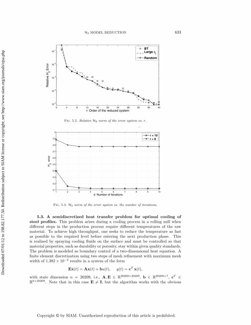
Copyright © by SIAM. Unauthorized reproduction of this article is prohibited.
H2 MODEL REDUCTION 633
0 4 8 12 16 20 24 28 32 36 4010
−5
10−4
10−3
10−2
10−1
r: Order of the reduced system
Rel
ativ
e H
2 Err
or
BTLarge φ
i
Random
Fig. 5.2. Relative H2 norm of the error system vs. r.
1 2 3 4 5 6 7 8 9 102.1
2.2
2.3
2.4
2.5
2.6
2.7
2.8
2.9
3
k: Number of iterations
H2 e
rror
r = 10r = 8
Fig. 5.3. H2 norm of the error system vs. the number of iterations.
5.3. A semidiscretized heat transfer problem for optimal cooling ofsteel profiles. This problem arises during a cooling process in a rolling mill whendifferent steps in the production process require different temperatures of the rawmaterial. To achieve high throughput, one seeks to reduce the temperature as fastas possible to the required level before entering the next production phase. Thisis realized by spraying cooling fluids on the surface and must be controlled so thatmaterial properties, such as durability or porosity, stay within given quality standards.The problem is modeled as boundary control of a two-dimensional heat equation. Afinite element discretization using two steps of mesh refinement with maximum meshwidth of 1.382 × 10⁻² results in a system of the form
Ex(t) = Ax(t) + bu(t), y(t) = cT x(t),
with state dimension n = 20209, i.e., A,E ∈ R20209×20209, b ∈ R
20209×7, cT ∈R
6×20209. Note that in this case E �= I, but the algorithm works with the obvious
Dow
nloa
ded
07/0
1/12
to 1
98.8
2.17
7.50
. Red
istr
ibut
ion
subj
ect t
o SI
AM
lice
nse
or c
opyr
ight
; see
http
://w
ww
.sia
m.o
rg/jo
urna
ls/o
jsa.
php

Copyright © by SIAM. Unauthorized reproduction of this article is prohibited.
634 S. GUGERCIN, A. C. ANTOULAS, AND C. BEATTIE
modifications. For details regarding the modeling, discretization, optimal controldesign, and model reduction for this example, see [29, 7, 8]. We consider the full-orderSISO system that associates the sixth input of this system with the second output.We apply our algorithm and reduce the order to r = 6. Amplitude Bode plots ofG(s) and Gr(s) are shown in Figure 5.4. The output response of Gr(s) is virtuallyindistinguishable from G(s) in the frequency range considered. IRKA converged in7 iteration steps in this case, although some interpolation points converged in thefirst 2–3 steps. The relative H∞ error obtained with our sixth order system was7.85 × 10−3. Note that in order to apply balanced truncation in this example, onewould need to solve two generalized Lyapunov equations (since E �= I) of order 20209.This presents a severe computational challenge, though there have been interestingapproaches to addressing it (e.g., [5]).
10−8
10−6
10−4
10−2
100
102
10−5
10−4
10−3
10−2
10−1
freq ω (rad/sec)
| H
(jω)|
H(s)H
r(s)
Fig. 5.4. Amplitude Bode plots of H(s) and Hr(s).
5.4. Successive substitution vs. Newton framework. In this section, wepresent two examples to show the effect of the Newton formulation for IRKA on twolow-order examples.
The first example is FOM-1 from section 5.1. For this example, for reductionto r = 1, the optimal shift is σ = 0.4952. We initiate both iterations, successivesubstitution and Newton frameworks, away from this optimal value with an initialselection σ0 = 104. Figure 5.5 illustrates how each process converges. As the figureshows, even though it takes almost 15 iterations with oscillations for the successivesubstitution framework to converge, the Newton formulation reaches the optimal shiftin 4 steps.
The second example in this section is a third-order model with a transfer function
G =−s2 + (7/4)s + 5/4
s3 + 2s2 + (17/16)s + 15/32.
One can exactly compute the optimal H2 reduced model for r = 1 as
Gr(s) =0.97197
s + 0.2727272
Dow
nloa
ded
07/0
1/12
to 1
98.8
2.17
7.50
. Red
istr
ibut
ion
subj
ect t
o SI
AM
lice
nse
or c
opyr
ight
; see
http
://w
ww
.sia
m.o
rg/jo
urna
ls/o
jsa.
php

Copyright © by SIAM. Unauthorized reproduction of this article is prohibited.
H2 MODEL REDUCTION 635
0 5 10 15 20 25 30 35 40 45 50−1
−0.5
0
0.5
1x 10
4 Shift Evolution− Successive Substutition Framework
k: Number of iterations
Shi
ft
1 2 3 4 5 6 7 8 9 10
100
104 Shift Evolution − Newton Iteration Framework
k: Number of Iterations
Shi
ft
Fig. 5.5. Comparison for FOM-1.
10 20 30 40 50 60 70 80 90 100−15
−10
−5
0
5
k: Number of Iterations
Shi
ft
Shift Evolution: Successive Substitution Framework with σ0 = 0.2
1 2 3 4 5 6 7 8 9 10 11
1
2000
k: Number of Iterations
Shi
ft
Shift Evolution: Newton Framework with σ0 = 2000
Fig. 5.6. Comparison for the random third-order model.
and easily show that this reduced model interpolates G(s) and its derivative at σ =0.2727272. We initiate Algorithm 4.1 with σ0 = 0.27, very close to the optimal shift.We initiate the Newton framework at σ0 = 2000, far away from the optimal solution.Convergence behavior of both models is depicted in Figure 5.6. The figure showsthat for this example, the successive substitution framework is divergent and indeed
Dow
nloa
ded
07/0
1/12
to 1
98.8
2.17
7.50
. Red
istr
ibut
ion
subj
ect t
o SI
AM
lice
nse
or c
opyr
ight
; see
http
://w
ww
.sia
m.o
rg/jo
urna
ls/o
jsa.
php

Copyright © by SIAM. Unauthorized reproduction of this article is prohibited.
636 S. GUGERCIN, A. C. ANTOULAS, AND C. BEATTIE
∂λ∂σ ≈ 1.3728. On the other hand, the Newton framework is able to converge to theoptimal solution in a small number of steps.
6. Conclusions. We have developed an interpolation-based rational Krylov al-gorithm that iteratively corrects interpolation locations until first-order H2 optimalityconditions are satisfied. The resulting method proves numerically effective and wellsuited for large-scale problems. A new derivation of the interpolation-based necessaryconditions is presented and shown to be equivalent to two other common frameworksfor H2 optimality.
Appendix.Lemma A.1. For any stable matrix M,
P.V.
∫ +∞
−∞(ıω − M)−1 dω
def= lim
L→∞
∫ L
−L
(ıω − M)−1 dω = πI.
Proof. Observe that for any L > 0,∫ L
−L
(ıω − M)−1 dω =
∫ L
−L
(−ıω − M)(ω2 + M2)−1 dω =
∫ L
−L
(−M)(ω2I + M2)−1 dω.
Fix a contour Γ contained in the open left half plane so that the interior of Γcontains all eigenvalues of M. Then
−M(ω2I + M2)−1 =1
2πı
∫Γ
−z
ω2 + z2(zI − M)−1 dz.
For any fixed value z in the left half plane,
P.V.
∫ +∞
−∞
dω
ıω − z= lim
L→∞
∫ L
−L
−z
ω2 + z2dω = π.
Thus,
limL→∞
∫ L
−L
(−M)(ω2I + M2)−1 dω =1
2πı
∫Γ
limL→∞
(∫ L
−L
−z
ω2 + z2dω
)(zI − M)−1 dz
=1
2πı
∫Γ
π (zI − M)−1 dz = πI.
REFERENCES
[1] A.C. Antoulas, Recursive modeling of discrete-time time series, in Linear Algebra for ControlTheory, P. Van Dooren and B. W. Wyman, eds., IMA Vol. Math. Appl. 62, Springer-Verlag,New York, 1993, pp. 1–20.
[2] A.C. Antoulas, Approximation of Large-Scale Dynamical Systems, Adv. Des. Control 6,SIAM, Philadelphia, 2005.
[3] A.C. Antoulas and J.C. Willems, A behavioral approach to linear exact modeling, IEEETrans. Automat. Control, 38 (1993), pp. 1776–1802.
[4] A.C. Antoulas, D.C. Sorensen, and S. Gugercin, A survey of model reduction methodsfor large scale systems, in Structured Matrices in Mathematics, Computer Science, andEngineering, I (Boulder, CO, 1999), Contemp. Math. 280, AMS, Providence, RI, 2001,pp. 193–219.
[5] J. Badia, P. Benner, R. Mayo, E.S. Quintana-Ortı, G. Quintana-Ortı, and J. Saak,Parallel order reduction via balanced truncation for optimal cooling of steel profiles, inProceedings of the 11th International European Conference on Parallel Processing, EuroPar2005, Lisbon, J. C. Cunha and P. D. Medeiros, eds., Lecture Notes in Comput. Sci. 3648,Springer-Verlag, Berlin, 2005, pp. 857–866.
Dow
nloa
ded
07/0
1/12
to 1
98.8
2.17
7.50
. Red
istr
ibut
ion
subj
ect t
o SI
AM
lice
nse
or c
opyr
ight
; see
http
://w
ww
.sia
m.o
rg/jo
urna
ls/o
jsa.
php

Copyright © by SIAM. Unauthorized reproduction of this article is prohibited.
H2 MODEL REDUCTION 637
[6] L. Baratchart, M. Cardelli, and M. Olivi, Identification and rational �2 approximation:A gradient algorithm, Automat., 27 (1991), pp. 413–418.
[7] P. Benner, Solving large-scale control problems, IEEE Control Systems Mag., 24 (2004),pp. 44–59.
[8] P. Benner and J. Saak, Efficient numerical solution of the LQR-problem for the heat equation,Proc. Appl. Math. Mech., 4 (2004), pp. 648–649.
[9] A.E. Bryson and A. Carrier, Second-order algorithm for optimal model order reduction, J.Guidance Control Dynam., 13 (1990), pp. 887–892.
[10] A. Bunse-Gerstner, D. Kubalinska, G. Vossen, and D. Wilczek, H2-optimal Model Re-duction for Large Scale Discrete Dynamical MIMO Systems, ZeTeM Technical Report 07-04, University of Bremen, 2007; available online from http://www.math.uni-bremen.de/zetem/reports/reports-liste.html#reports2007.
[11] C. De Villemagne and R. Skelton, Model reduction using a projection formulation, Internat.J. Control, 40 (1987), pp. 2141–2169.
[12] P. Feldman and R.W. Freund, Efficient linear circuit analysis by Pade approximation via aLanczos method, IEEE Trans. Computer-Aided Design, 14 (1995), pp. 639–649.
[13] P. Fulcheri and M. Olivi, Matrix rational H2 approximation: A gradient algorithm basedon Schur analysis, SIAM J. Control Optim., 36 (1998), pp. 2103–2127.
[14] D. Gaier, Lectures on Complex Approximation, Birkhauser, Boston, 1987.[15] K. Gallivan, E. Grimme, and P. Van Dooren, A rational Lanczos algorithm for model
reduction, Numer. Algorithms, 2 (1996), pp. 33–63.[16] K. Gallivan, P. Van Dooren, and E. Grimme, On some recent developments in projection-
based model reduction, in ENUMATH 97 (Heidelberg), World Scientific, River Edge, NJ,1998, pp. 98–113.
[17] E.J. Grimme, Krylov Projection Methods for Model Reduction, Ph.D. thesis, University ofIllinois, Urbana-Champaign, Urbana, IL, 1997.
[18] S. Gugercin, Projection Methods for Model Reduction of Large-Scale Dynamical Systems,Ph.D. thesis, Rice University, Houston, TX, 2002.
[19] S. Gugercin and A.C. Antoulas, A comparative study of 7 model reduction algorithms, inProceedings of the 39th IEEE Conference on Decision and Control, Sydney, 2000, pp. 2367–2372.
[20] S. Gugercin and A.C. Antoulas, An H2 error expression for the Lanczos procedure, inProceedings of the 42nd IEEE Conference on Decision and Control, 2003, pp. 1869–1872.
[21] Y. Halevi, Frequency weighted model reduction via optimal projection, in Proceedings of the29th IEEE Conference on Decision and Control, 1990, pp. 2906–2911.
[22] D.C. Hyland and D.S. Bernstein, The optimal projection equations for model reductionand the relationships among the methods of Wilson, Skelton, and Moore, IEEE Trans.Automat. Control, 30 (1985), pp. 1201–1211.
[23] J.G. Korvink and E.B. Rudyni, Oberwolfach benchmark collection, in Dimension Reduction ofLarge-Scale Systems, P. Benner, G. Golub, V. Mehrmann, and D. Sorensen, eds., LectureNotes in Comput. Sci. Engrg. 45, Springer-Verlag, New York, 2005.
[24] D. Kubalinska, A. Bunse-Gerstner, G. Vossen, and D. Wilczek, H2-optimal interpolationbased model reduction for large-scale systems, in Proceedings of the 16th InternationalConference on System Science, Wroclaw, Poland, 2007.
[25] A. Lepschy, G.A. Mian, G. Pinato, and U. Viaro, Rational L2 approximation: A non-gradient algorithm, in Proceedings of the 30th IEEE Conference on Decision and Control,1991, pp. 2321–2323.
[26] L. Meier and D.G. Luenberger, Approximation of linear constant systems, IEEE Trans.Automat. Control, 12 (1967), pp. 585–588.
[27] B.C. Moore, Principal component analysis in linear system: Controllability, observability andmodel reduction, IEEE Trans. Automat. Control, 26 (1981), pp. 17–32.
[28] C.T. Mullis and R.A. Roberts, Synthesis of minimum roundoff noise fixed point digitalfilters, IEEE Trans. Circuits Systems, CAS-23 (1976), pp. 551–562.
[29] T. Penzl, Algorithms for model reduction of large dynamical systems, Linear Algebra Appl.,415 (2006), pp. 322–343.
[30] L.T. Pillage and R.A. Rohrer, Asymptotic waveform evaluation for timing analysis, IEEETrans. Computer-Aided Design, 9 (1990), pp. 352–366.
[31] V. Raghavan, R.A. Rohrer, L.T. Pillage, J.Y. Lee, J.E. Bracken, and M.M. Alaybeyi,AWE inspired, in Proceedings of the IEEE Custom Integrated Circuits Conference, 1993,pp. 18.1.1–18.1.8.
[32] F. Riesz and B. Sz.-Nagy, Functional Analysis, Ungar, New York, 1955.[33] A. Ruhe, Rational Krylov algorithms for nonsymmetric eigenvalue problems II: Matrix pairs,
Linear Algebra Appl., 197 (1994), pp. 283–295.
Dow
nloa
ded
07/0
1/12
to 1
98.8
2.17
7.50
. Red
istr
ibut
ion
subj
ect t
o SI
AM
lice
nse
or c
opyr
ight
; see
http
://w
ww
.sia
m.o
rg/jo
urna
ls/o
jsa.
php

Copyright © by SIAM. Unauthorized reproduction of this article is prohibited.
638 S. GUGERCIN, A. C. ANTOULAS, AND C. BEATTIE
[34] J.T. Spanos, M.H. Milman, and D.L. Mingori, A new algorithm for L2 optimal model re-duction, Automat., 28 (1992), pp. 897–909.
[35] P. Van Dooren, K.A. Gallivan, and P.-A. Absil, H2 optimal model reduction of MIMOsystems, Appl. Math. Lett., to appear; doi:10.1016/j.aml.2007.09.015.
[36] D.A. Wilson, Optimum solution of model reduction problem, Proc. IEE-D, 117 (1970),pp. 1161–1165.
[37] W.-Y. Yan and J. Lam, An approximate approach to H2 optimal model reduction, IEEE Trans.Automat. Control, 44 (1999), pp. 1341–1358.
[38] A. Yousouff and R.E. Skelton, Covariance equivalent realizations with applications to modelreduction of large-scale systems, in Control and Dynamic Systems, Vol. 22, C. T. Leondes,ed., Academic Press, New York, 1985, pp. 273–348.
[39] A. Yousouff, D.A. Wagie, and R.E. Skelton, Linear system approximation via covarianceequivalent realizations, J. Math. Anal. Appl., 196 (1985), pp. 91–115.
[40] D. Zigic, L. Watson, and C. Beattie, Contragredient transformations applied to the optimalprojection equations, Linear Algebra Appl., 188/189 (1993), pp. 665–676.
Dow
nloa
ded
07/0
1/12
to 1
98.8
2.17
7.50
. Red
istr
ibut
ion
subj
ect t
o SI
AM
lice
nse
or c
opyr
ight
; see
http
://w
ww
.sia
m.o
rg/jo
urna
ls/o
jsa.
php


![Model Order Reduction for Networked Control Systems...Model Order Reduction Iterative Rational Krylov Algorithm (IRKA) [ Gugercin et al. '08 ] Fixed-point iteration algorithm, based](https://img.pdfslide.us/doc/110x75/60b2c7a9c81c401954395c0c/model-order-reduction-for-networked-control-systems-model-order-reduction-iterative.jpg)