functional analysis master - Rhodes University otherwise stated, we shall denote by R the ﬁeld of real numbers and by C the ﬁeld of complex numbers. Let F denote either R or C

FUNCTIONAL ANALYSIS NOTES

(2011)

Mr. Andrew Pinchuck

Department of Mathematics (Pure & Applied)

Rhodes University

Contents

Introduction 1

1 Linear Spaces 2

1.1 Introducton . . . . . . . . . . . . . . . . . . . . . . . . . . . . . . . . . . . . . . . . . . 2

1.2 Subsets of a linear space . . . . . . . . . . . . . . . . . . . . . . . . . . . . . . . . . . . 5

1.3 Subspaces and Convex Sets . . . . . . . . . . . . . . . . . . . . . . . . . . . . . . . . . . 5

1.4 Quotient Space . . . . . . . . . . . . . . . . . . . . . . . . . . . . . . . . . . . . . . . . 7

1.5 Direct Sums and Projections . . . . . . . . . . . . . . . . . . . . . . . . . . . . . . . . . 8

1.6 The Holder and Minkowski Inequalities . . . . . . . . . . . . . . . . . . . . . . . . . . . 9

2 Normed Linear Spaces 13

2.1 Preliminaries . . . . . . . . . . . . . . . . . . . . . . . . . . . . . . . . . . . . . . . . . 13

2.2 Quotient Norm and Quotient Map . . . . . . . . . . . . . . . . . . . . . . . . . . . . . . 18

2.3 Completeness of Normed Linear Spaces . . . . . . . . . . . . . . . . . . . . . . . . . . . 19

2.4 Series in Normed Linear Spaces . . . . . . . . . . . . . . . . . . . . . . . . . . . . . . . 24

2.5 Bounded, Totally Bounded, and Compact Subsets of a Normed Linear Space . . . . . . . 26

2.6 Finite Dimensional Normed Linear Spaces . . . . . . . . . . . . . . . . . . . . . . . . . . 28

2.7 Separable Spaces and Schauder Bases . . . . . . . . . . . . . . . . . . . . . . . . . . . . 32

3 Hilbert Spaces 36

3.1 Introduction . . . . . . . . . . . . . . . . . . . . . . . . . . . . . . . . . . . . . . . . . . 36

3.2 Completeness of Inner Product Spaces . . . . . . . . . . . . . . . . . . . . . . . . . . . . 42

3.3 Orthogonality . . . . . . . . . . . . . . . . . . . . . . . . . . . . . . . . . . . . . . . . . 42

3.4 Best Approximation in Hilbert Spaces . . . . . . . . . . . . . . . . . . . . . . . . . . . . 45

3.5 Orthonormal Sets and Orthonormal Bases . . . . . . . . . . . . . . . . . . . . . . . . . . 49

4 Bounded Linear Operators and Functionals 62

4.1 Introduction . . . . . . . . . . . . . . . . . . . . . . . . . . . . . . . . . . . . . . . . . . 62

4.2 Examples of Dual Spaces . . . . . . . . . . . . . . . . . . . . . . . . . . . . . . . . . . . 72

4.3 The Dual Space of a Hilbert Space . . . . . . . . . . . . . . . . . . . . . . . . . . . . . . 77

5 The Hahn-Banach Theorem and its Consequences 81

5.1 Introduction . . . . . . . . . . . . . . . . . . . . . . . . . . . . . . . . . . . . . . . . . . 81

5.2 Consequences of the Hahn-Banach Extension Theorem . . . . . . . . . . . . . . . . . . . 85

5.3 Bidual of a normed linear space and Reflexivity . . . . . . . . . . . . . . . . . . . . . . . 88

5.4 The Adjoint Operator . . . . . . . . . . . . . . . . . . . . . . . . . . . . . . . . . . . . . 90

5.5 Weak Topologies . . . . . . . . . . . . . . . . . . . . . . . . . . . . . . . . . . . . . . . 91

1

2011 FUNCTIONAL ANALYSIS ALP

6 Baire’s Category Theorem and its Applications 99

6.1 Introduction . . . . . . . . . . . . . . . . . . . . . . . . . . . . . . . . . . . . . . . . . . 99

6.2 Uniform Boundedness Principle . . . . . . . . . . . . . . . . . . . . . . . . . . . . . . . 101

6.3 The Open Mapping Theorem . . . . . . . . . . . . . . . . . . . . . . . . . . . . . . . . . 102

6.4 Closed Graph Theorem . . . . . . . . . . . . . . . . . . . . . . . . . . . . . . . . . . . . 104

2


Introduction

These course notes are adapted from the original course notes written by Prof. Sizwe Mabizela when

he last gave this course in 2006 to whom I am indebted. I thus make no claims of originality but have made

several changes throughout. In particular, I have attempted to motivate these results in terms of applications

in science and in other important branches of mathematics.

Functional analysis is the branch of mathematics, specifically of analysis, concerned with the study of

vector spaces and operators acting on them. It is essentially where linear algebra meets analysis. That is,

an important part of functional analysis is the study of vector spaces endowed with topological structure.

Functional analysis arose in the study of tansformations of functions, such as the Fourier transform, and in

the study of differential and integral equations. The founding and early development of functional analysis

is largely due to a group of Polish mathematicians around Stefan Banach in the first half of the 20th century

but continues to be an area of intensive research to this day. Functional analysis has its main applications in

differential equations, probability theory, quantum mechanics and measure theory amongst other areas and

can best be viewed as a powerful collection of tools that have far reaching consequences.

As a prerequisite for this course, the reader must be familiar with linear algebra up to the level of a

standard second year university course and be familiar with real analysis. The aim of this course is to

introduce the student to the key ideas of functional analysis. It should be remembered however that we

only scratch the surface of this vast area in this course. We examine normed linear spaces, Hilbert spaces,

bounded linear operators, dual spaces and the most famous and important results in functional analysis

such as the Hahn-Banach theorem, Baires category theorem, the uniform boundedness principle, the open

mapping theorem and the closed graph theorem. We attempt to give justifications and motivations for the

ideas developed as we go along.

Throughout the notes, you will notice that there are exercises and it is up to the student to work through

these. In certain cases, there are statements made without justification and once again it is up to the student

to rigourously verify these results. For further reading on these topics the reader is referred to the following

texts:

� G. BACHMAN, L. NARICI, Functional Analysis, Academic Press, N.Y. 1966.

� E. KREYSZIG, Introductory Functional Analysis, John Wiley & sons, New York-Chichester-Brisbane-

Toronto, 1978.

� G. F. SIMMONS, Introduction to topology and modern analysis, McGraw-Hill Book Company, Sin-

gapore, 1963.

� A. E. TAYLOR, Introduction to Functional Analysis, John Wiley & Sons, N. Y. 1958.

I have also found Wikipedia to be quite useful as a general reference.

1

Chapter 1

Linear Spaces

1.1 Introducton

In this first chapter we review the important notions associated with vector spaces. We also state and prove

some well known inequalities that will have important consequences in the following chapter.

Unless otherwise stated, we shall denote by R the field of real numbers and by C the field of complex

numbers. Let F denote either R or C.

1.1.1 Definition

A linear space over a field F is a nonempty set X with two operations

C W X � X ! X (called addition); and

� W F � X ! X (called multiplication)

satisfying the following properties:

[1] x C y 2 X whenever x; y 2 X ;

[2] x C y D y C x for all x; y 2 X ;

[3] There exists a unique element in X , denoted by 0, such that x C 0 D 0C x D x for all x 2 X ;

[4] Associated with each x 2 X is a unique element in X , denoted by �x, such that x C .�x/ D�x C x D 0;

[5] .x C y/ C z D x C .y C z/ for all x; y; z 2 X ;

[6] ˛ � x 2 X for all x 2 X and for all ˛ 2 F;

[7] ˛ � .x C y/ D ˛ � x C ˛ � y for all x; y 2 X and all ˛ 2 F;

[8] .˛ C ˇ/ � x D ˛ � x C ˇ � x for all x 2 X and all ˛; ˇ 2 F;

[9] .˛ˇ/ � x D ˛ � .ˇ � x/ for all x 2 X and all ˛; ˇ 2 F;

[10] 1 � x D x for all x 2 X .

We emphasize that a linear space is a quadruple .X;F;C; �/ where X is the underlying set, F a field,Caddition, and � multiplication. When no confusion can arise we shall identify the linear space .X;F;C; �/with the underlying set X . To show that X is a linear space, it suffices to show that it is closed under

addition and scalar multiplication operations. Once this has been shown, it is easy to show that all the other

axioms hold.

2


1.1.2 Definition

A real (resp. complex) linear space is a linear space over the real (resp. complex) field.

A linear space is also called a vector space and its elements are called vectors.

1.1.3 Examples

[1] For a fixed positive integer n, let X D Fn D fx D .x1; x2; : : : ; xn/ W xi 2 F; i D1; 2; : : : ; ng – the set of all n-tuples of real or complex numbers. Define the operations

of addition and scalar multiplication pointwise as follows: For all x D .x1; x2; : : : ; xn/;

y D .y1; y2; : : : ; yn/ in Fn and ˛ 2 F,

x C y D .x1 C y1; x2 C y2; : : : ; xn C yn/

˛ � x D .˛x1; ˛x2; : : : ; ˛xn/:

Then Fn is a linear space over F.

[2] Let X D C Œa; b� D f x W Œa; b�! F j x is continuous g. Define the operations of addition and

scalar multiplication pointwise: For all x; y 2 X and all ˛ 2 R, define

.x C y/.t/ D x.t/C y.t/ and

.˛ � x/.t/ D ˛x.t/

�for all t 2 Œa; b�:

Then CŒa; b� is a real vector space.

Sequence Spaces: Informally, a sequence in X is a list of numbers indexed by N. Equivalently,

a sequence in X is a function x W N ! X given by n 7! x.n/ D xn. We shall denote asequence x1; x2; : : : by

x D .x1; x2; : : :/ D .xn/11 :

[3] The sequence space s. Let s denote the set of all sequences x D .xn/11

of real or complexnumbers. Define the operations of addition and scalar multiplication pointwise: For all x D.x1; x2; : : :/, y D .y1; y2; : : :/ 2 s and all ˛ 2 F, define

x C y D .x1 C y1; x2 C y2; : : :/

˛ � x D .˛x1; ˛x2; : : :/:

Then s is a linear space over F.

[4] The sequence space `1 . Let `1 D `1.N/ denote the set of all bounded sequences of real or

complex numbers. That is, all sequences x D .xn/11

such that

supi2N

jxi j <1:

Define the operations of addition and scalar multiplication pointwise as in example (3). Then

`1 is a linear space over F.

[5] The sequence space p D p.N/; 1 � p < 1. Let p denote the set of all sequences

x D .xn/11

of real or complex numbers satisfying the condition

1X

iD1

jxi jp <1:

Define the operations of addition and scalar multiplication pointwise: For all x D .xn/, y D.yn/ in p and all ˛ 2 F, define

x C y D .x1 C y1; x2 C y2; : : :/

˛ � x D .˛x1; ˛x2; : : :/:

3


Then p is a linear space over F.

Proof. Let x D .x1; x2; : : :/, y D .y1; y2; : : :/ 2 p . We must show that x C y 2 p . Since,

for each i 2 N,

jxi C yi jp � Œ2 maxfjxij; jyijg�p � 2p maxfjxijp ; jyijpg � 2p .jxijp C jyi jp/ ;

it follows that1X

iD1

jxi C yi jp � 2p

1X

iD1

jxijp C1X

iD1

jyi jp!<1:

Thus, x C y 2 p . Also, if x D .xn/ 2 p and ˛ 2 F, then

1X

iD1

j˛xijp D j˛jp1X

iD1

jxijp <1:

That is, ˛ � x 2 p .

[6] The sequence space c D c.N/. Let c denote the set of all convergent sequences x D .xn/11

of

real or complex numbers. That is, c is the set of all sequences x D .xn/11

such that limn!1

xn

exists. Define the operations of addition and scalar multiplication pointwise as in example

(3). Then c is a linear space over F.

[7] The sequence space c0 D c0.N/. Let c0 denote the set of all sequences x D .xn/11

of real

or complex numbers which converge to zero. That is, c0 is the space of all sequencesx D .xn/

11

such that limn!1

xn D 0. Define the operations of addition and scalar multiplication

pointwise as in example (3). Then c0 is a linear space over F.

[8] The sequence space `0 D `0.N/. Let `0 denote the set of all sequences x D .xn/11 of real or

complex numbers such that xi D 0 for all but finitely many indices i . Define the operations

of addition and scalar multiplication pointwise as in example (3). Then `0 is a linear space

over F.

4


1.2 Subsets of a linear space

Let X be a linear space over F; x 2 X and A and B subsets of X and � 2 F. We shall denote by

x CA WD fx C a W a 2 Ag;AC B WD faC b W a 2 A; b 2 Bg;

�A WD f�a W a 2 Ag:

1.3 Subspaces and Convex Sets

1.3.1 Definition

A subset M of a linear space X is called a linear subspace of X if

(a) x C y 2M for all x; y 2M , and

(b) �x 2M for all x 2M and for all � 2 F.

Clearly, a subset M of a linear space X is a linear subspace if and only if M CM �M and �M �M

for all � 2 F.

1.3.2 Examples

[1] Every linear space X has at least two distinguished subspaces: M D f0g and M D X .

These are called the improper subspaces of X . All other subspaces of X are called the

proper subspaces.

[2] Let X D R2. Then the nontrivial linear subspaces of X are straight lines through the origin.

[3] M D fx D .0; x2; x3; : : : ; xn/ W xi 2 R; i D 2; 3; : : : ; ng is a subspace of Rn.

[4] M D fx W Œ�1; 1�! R; x continuous and x.0/ D 0g is a subspace of CŒ�1; 1�.

[5] M D fx W Œ�1; 1�! R; x continuous and x.0/ D 1 g is not a subspace of CŒ�1; 1�.

[6] Show that c0 is a subspace of c.

1.3.3 Definition

Let K be a subset of a linear space X . The linear hull of K, denoted by lin.K/ or span.K/, is the

intersection of all linear subspaces of X that contain K.

The linear hull of K is also called the linear subspace of X spanned (or generated) by K.

It is easy to check that the intersection of a collection of linear subspaces of X is a linear subspace of

X . It therefore follows that the linear hull of a subset K of a linear space X is again a linear subspace of X .

In fact, the linear hull of a subset K of a linear space X is the smallest linear subspace of X which contains

K.

1.3.4 Proposition

Let K be a subset of a linear space X . Then the linear hull of K is the set of all finite linear combinations

of elements of K. That is,

lin.K/ D

8<:

nX

jD1

�jxj j x1; x2; : : : ; xn 2 K; �1; �2; : : : ; �n 2 F; n 2 N

9=; :

5


Proof. Exercise. �

1.3.5 Definition

[1] A subset fx1; x2; : : : ; xng of a linear space X is said to be linearly independent if the equation

˛1x1C ˛2x2 C � � � C ˛nxn D 0

only has the trivial solution ˛1 D ˛2 D � � � D ˛n D 0. Otherwise, the set fx1; x2; : : : ; xng is

linearly dependent.

[2] A subset K of a linear space X is said to be linearly independent if every finite subset fx1; x2; : : : ; xngof K is linearly independent.

1.3.6 Definition

If fx1; x2; : : : ; xng is a linearly independent subset of X and

X D linfx1; x2; : : : ; xng, then X is said to have dimension n. In this case we say that fx1; x2; : : : ; xngis a basis for the linear space X . If a linear space X does not have a finite basis, we say that it is infinite-

dimensional.

1.3.7 Examples

[1] The space Rn has dimension n. Its standard basis is fe1; e2; : : : ; eng, where, for eachj D 1; 2; : : : ; n, ej is an n-tuple of real numbers with 1 in the j -th position and zeroes

elsewhere; i.e.,

ej D .0; 0; : : : ; 1; 0; : : : ; 0/; where 1 occurs in the j -th position.

[2] The space Pn of polynomials of degree at most n has dimension nC 1. Its standard basis is

f1; t; t2; : : : ; tng.

[3] The function space CŒa; b� is infinite-dimensional.

[4] The spaces p , with 1 � p � 1, are infinite-dimensional.

1.3.8 Definition

Let K be a subset of a linear space X . We say that

(a) K is convex if �x C .1 � �/y 2 K whenever x; y 2 K and � 2 Œ0; 1�;

(b) K is balanced if �x 2 K whenever x 2 K and j�j � 1;

(c) K is absolutely convex if K is convex and balanced.

1.3.9 Remark

[1] It is easy to verify that K is absolutely convex if and only if �x C�y 2 K whenever x; y 2 K

and j�j C j�j � 1.

[2] Every linear subspace is absolutely convex.

1.3.10 Definition

Let S be a subset of the linear space X . The convex hull of S , denoted co.S/, is the intersection

of all convex sets in X which contain S .

Since the intersection of convex sets is convex, it follows that co.S/ is the smallest convex set which

contains S . The following result is an alternate characterization of co.S/.

6


1.3.11 Proposition

Let S be a nonempty subset of a linear space X . Then co.S/ is the set of all convex combinations of

elements of S . That is,

co.S/ D

8<:

nX

jD1

�jxj j x1; x2; : : : ; xn 2 S; �j � 0 8 j D 1; 2; : : : ; n;

nX

jD1

�j D 1; n 2 N

9=; :

Proof. Let C denote the set of all convex combinations of elements of S . That is,

C D

8<:

nX

jD1

�jxj j x1; x2; : : : ; xn 2 S; �j � 0 8 j D 1; 2; : : : ; n;

nX

jD1

�j D 1; n 2 N

9=; :

Let x; y 2 C and 0 � � � 1. Then x DnX

1

�ixi; y DmX

1

�iyi , where �i; �i � 0,

nX

1

�i D 1,

mX

1

�i D 1, and xi ; yi 2 S . Thus

�x C .1 � �/y DnX

1

��ixi CmX

1

.1 � �/�iyi

is a linear combination of elements of S , with nonnegative coefficients, such that

nX

1

��i CmX

1

.1 � �/�i D �nX

1

�i C .1 � �/mX

1

�i D �C .1 � �/ D 1:

That is, �x C .1 � �/y 2 C and C is convex. Clearly S � C . Hence co.S/ � C .

We now prove the inclusion C � co.S/. Note that, by definition, S � co.S/. Let x1; x2 2 S ,

�1 � 0; �2 � 0 and �1 C �2 D 1. Then, by convexity of co.S/, �1x1 C �2x2 2 co.S/. Assume thatn�1X

1

�ixi 2 co.S/ whenever x1; x2; : : : ; xn�1 2 S , �j � 0, j D 1; 2; : : : ; n � 1 and

n�1X

jD1

�j D 1. Let

x1; x2; : : : ; xn 2 S and �1; �2; : : : ; �n be such that �j � 0, j D 1; 2; : : : ; n and

nX

jD1

�j D 1. If

n�1X

jD1

�j D 0, then �n D 1. Hence

nX

1

�jxj D �nxn 2 co.S/. Assume that ˇ Dn�1X

jD1

�j > 0. Then�j

ˇ� 0

for all j D 1; 2; : : : ; n � 1 and

n�1X

jD1

�j

ˇD 1. By the induction assumption,

n�1X

jD1

�j

ˇxj 2 co.S/. Hence

nX

jD1

�jxj D ˇ

0@

n�1X

jD1

�j

ˇxj

1AC �nxn 2 co.S/:

Thus C � co.S/. �

1.4 Quotient Space

Let M be a linear subspace of a linear space X over F. For all x; y 2 X , define

x � y.mod M / ” x � y 2M:

7


It is easy to verify that� defines an equivalence relation on X .

For x 2 X , denote by

Œx� WD fy 2 X W x � y.mod M /g D fy 2 X W x � y 2M g D x CM;

the coset of x with respect to M . The quotient space X=M consists of all the equivalence classes Œx�,

x 2 X . The quotient space is also called a factor space.

1.4.1 Proposition

Let M be a linear subspace of a linear space X over F. For x; y 2 X and � 2 F, define the operations

Œx�C Œy� D Œx C y� and � � Œx� D Œ� � x�:

Then X=M is a linear space with respect to these operations.


Note that the linear operations on X=M are equivalently given by: For all x; y 2 X and � 2 F,

.x CM /C .y CM / D x C y CM and �.x CM / D �x CM:

1.4.2 Definition

Let M be a linear subspace of a linear space X over F. The codimension of M in X is defined as the

dimension of the quotient space X=M . It is denoted by codim.M / D dim.X=M /.

Clearly, if X DM , then X=M D f0g and so codim.X / D 0.

1.5 Direct Sums and Projections

1.5.1 Definition

Let M and N be linear subspaces of a linear space X over F. We say that X is a direct sum of M and N

if

X DM CN and M \N D f0g:If X is a direct sum of M and N , we write X D M ˚ N . In this case, we say that M (resp. N ) is an

algebraic complement of N (resp. M ).

1.5.2 Proposition

Let M and N be linear subspaces of a linear space X over F. If X D M ˚ N , then each x 2 X has a

unique representation of the form x D mC n for some m 2M and n 2 N .


Let M and N be linear subspaces of a linear space X over F such that X D M ˚ N . Then

codim.M / Ddim.N /. Also, since X DM ˚N , dim.X / Ddim.M /Cdim.N /. Hence

dim.X / D dim.M /C codim.M /:

It follows that if dim.X / <1, then codim.M / Ddim.X /�dim.M /.

The operator P W X ! X is called an algebraic projection if P is linear (i.e., P .˛xCy/ D ˛PxCPy

for all x; y 2 X and ˛ 2 F) and P 2 D P , i.e., P is idempotent.

8


1.5.3 Proposition

Let M and N be linear subspaces of a linear space X over F such that X DM ˚N . Define P W X ! X

by P .x/ D m, where x D mC n, with m 2 M and n 2 N . Then P is an algebraic projection of X onto

M along N . Moreover M D P .X / and N D .I � P /.X / D ker.P /.

Conversely, if P W X ! X is an algebraic projection, then X D M ˚ N , where M D P .X / and

N D .I � P /.X / D ker.P /.

Proof. Linearity of P: Let x D m1 C n1 and y D m2 C n2, where m1;m2 2 M and n1; n2 2 N . For

˛ 2 F,

P .˛x C y/ D P ..˛m1 Cm2/C .˛n1 C n2// D ˛m1 Cm2 D ˛Px C Py:

Idempotency of P: Since m D m C 0, with m 2 M and 0 2 N , we have that Pm D m and hence

P 2x D Pm D m D Px. That is, P 2 D P .

Finally, n D x � m D .I � P /x. Hence N D .I � P /.X /. Also, Px D 0 if and only if x 2 N , i.e.,

ker.P / D N .

Conversely, let x 2 X and set m D Px and n D .I � P /x. Then x D m C n, where m 2 M and

n 2 N . We show that this representation is unique. Indeed, if x D m1 C n1 where m1 2 M and n1 2 N ,

then m1 D Pu and n1 D .I � P /v for some u; v 2 X . Since P 2 D P , it follows that Pm1 D m1 and

Pn1 D 0. Hence m D Px D Pm1 C Pn1 D Pm1 D m1. Similarly n D n1. �

1.6 The Holder and Minkowski Inequalities

We now turn our attention to three important inequalities. The first two are required mainly to prove the

third which is required for our discussion about normed linear spaces in the subsequent chapter.

1.6.1 Definition

Let p and q be positive real numbers. If 1 < p <1 and1

pC 1

qD 1, or if p D 1 and q D 1, or if p D1

and q D 1, then we say that p and q are conjugate exponents.

1.6.2 Lemma

(Young’s Inequality). Let p and q be conjugate exponents, with 1 < p; q <1 and ˛; ˇ � 0. Then

˛ˇ � ˛p

pC ˇq

q:

Proof. If p D 2 D q, then the inequality follows from the fact that .˛�ˇ/2 � 0. Notice also, that if ˛ D 0

or ˇ D 0, then the inequality follows trivially.

If p 6D 2, then consider the function f W Œ0;1/! R given by

f .˛/ D ˛p

pC ˇq

q� ˛ˇ; for fixed ˇ > 0:

Then, f 0.˛/ D ˛p�1 � ˇ D 0 when ˛p�1 D ˇ. That is, when ˛ D ˇ1

p�1 D ˇqp > 0. We now apply

the second derivative test to the critical point ˛ D ˇqp .

f 00.˛/ D .p � 1/˛p�2 > 0; for all ˛ 2 .0;1/:

9


Thus, we have a global minimum at ˛ D ˇqp : It is easily verified that

0 D f .ˇqp / � f .˛/ D ˛p

pC ˇq

q� ˛ˇ, ˛ˇ � ˛p

pC ˇq

q;

for each ˛ 2 Œ0;1/.�

1.6.3 Theorem

(Holder’s Inequality for sequences). Let .xn/ 2 p and .yn/ 2 `q , where p > 1 and 1=p C 1=q D 1.

Then1X

kD1

jxkyk j � 1X

kD1

jxk jp! 1

p 1X

kD1

jyk jq! 1

q

:

Proof. If

1X

kD1

jxk jp D 0 or

1X

kD1

jyk jq D 0, then the inequality holds. Assume that

1X

kD1

jxk jp 6D 0 and

1X

kD1

jyk jq 6D 0. Then for k D 1; 2; : : :, we have, by Lemma 1.6.2, that

jxk j�P1

kD1 jxk jp� 1

p

� jyk j�P1

kD1 jyk jq� 1

q

� 1

p

jxkjpP1kD1 jxk jp

C 1

q

jyk jqP1kD1 jyk jq

:

Hence, P1kD1 jxkyk j

�P1kD1 jxkjp

� 1p�P1

kD1 jyk jq� 1

q

� 1

pC 1

qD 1:

That is,

1X

kD1

jxkyk j � 1X

kD1

jxk jp! 1

p 1X

kD1

jyk jq! 1

q

: �

1.6.4 Theorem

(Minkowski’s Inequality for sequences). Let p > 1 and .xn/ and .yn/ sequences in p. Then

1X

kD1

jxk C yk jp! 1

p

� 1X

kD1

jxk jp! 1

p

C 1X

kD1

jyk jp! 1

p

:

10


Proof. Let q D p

p � 1. If

1X

kD1

jxk C yk jp D 0, then the inequality holds. We therefore assume that

1X

kD1

jxk C yk jp 6D 0. Then

1X

kD1

jxk C yk jp D1X

kD1

jxk C yk jp�1jxk C yk j

�1X

kD1

jxk C yk jp�1jxk j C1X

kD1

jxk C yk jp�1jyk j

� 1X

kD1

jxk C yk j.p�1/q

! 1q

24 1X

kD1

jxkjp! 1

p

C 1X

kD1

jyk jp! 1

p

35

D 1X

kD1

jxk C yk jp! 1

q

24 1X

kD1

jxk jp! 1

p

C 1X

kD1

jyk jp! 1

p

35 :

Dividing both sides by

1X

kD1

jxk C yk jp! 1

q

, we have

1X

kD1

jxk C yk jp! 1

p

D 1X

kD1

jxk C yk jp!1� 1

q

� 1X

kD1

jxk jp! 1

p

C 1X

kD1

jyk jp! 1

p

: �

1.6.5 Exercise

[1] Show that the set of all n�m real matrices is a real linear space.

[2] Show that a subset M of a linear space X is a linear subspace if and only if ˛x C ˇy 2 M

for all x; y 2M and all ˛; ˇ 2 F.

[3] Prove Proposition 1.3.4

[4] Prove Proposition 1.4.1.

[5] Prove Proposition 1.5.2.

[6] Show that c0 is a linear subspace of the linear space `1.

[7] Which of the following subsets are linear subspaces of the linear space CŒ�1; 1�?

(a) M1 D fx 2 CŒ�1; 1� W x.�1/ D x.1/g.

(b) M2 D fx 2 CŒ�1; 1� W1Z

�1

x.t/dt D 1g.

(c) M3 D fx 2 CŒ�1; 1� W jx.t2/ � x.t1/j � jt2 � t1j for all t1; t2 2 Œ�1; 1�g.

11


[8] Show that if fM�g is a family of linear subspaces of a linear space X , then M D \�M� is alinear subspace of X .

If M and N are linear subspaces of a linear space X , under what condition(s) is M [ N a

linear subspace of X ?

12

Chapter 2

Normed Linear Spaces

2.1 Preliminaries

For us to have a meaningful notion of convergence it is necessary for the Linear space to have a notion

distance and therefore a topology defined on it. This leads us to the definition of a norm which induces a

metric topology in a natural way.

2.1.1 Definition

A norm on a linear space X is a real-valued function k�k W X ! R which satisfies the following properties:

For all x; y 2 X and � 2 F,

N1. kxk � 0;

N2. kxk D 0 ” x D 0;

N3. k�xk D j�jkxk;

N4. kx C yk � kxk C kyk (Triangle Inequality).

A normed linear space is a pair .X; k � k/, where X is a linear space and k � k a norm on X . The number

kxk is called the norm or length of x.

Unless there is some danger of confusion, we shall identify the normed linear space .X; k � k/ with the

underlying linear space X .

2.1.2 Examples

(Examples of normed linear spaces.)

[1] Let X D F. For each x 2 X , define kxk D jxj. Then .X; k � k/ is a normed linear space.

We give the proof for X D C. Properties N1 -N3 are easy to verify. We only verify N4. Let

x; y 2 C. Then

kx C yk2 D jx C yj2 D .x C y/.x C y/ D .x C y/.x C y/ D xx C yx C xy C yy

D jxj2 C xy C xy C jyj2 D jxj2C 2Re.xy/C jyj2

� jxj2 C 2jxyj C jyj2 D jxj2 C 2jxjjyj C jyj2

D jxj2 C 2jxjjyj C jyj2

D .jxj C jyj/2 D .kxk C kyk/2 :

Taking the positive square root both sides yields N4. �

13


[2] Let n be a natural number and X D Fn. For each x D .x1; x2; : : : ; xn/ 2 X , define

kxkp D

nX

iD1

jxijp! 1

p

; for 1 � p <1; and

kxk1 D max1�i�n

jxi j:

Then .X; k � kp/ and .X; k � k1/ are normed linear spaces. We give a detailed proof that

.X; k � kp/ is a normed linear space for 1 � p <1.

N1. For each 1 � i � n,

jxi j � 0 )nX

iD1

jxijp � 0 )

nX

iD1

jxi jp! 1

p

� 0 ) kxkp � 0:

N2. For any x 2 X ,

kxkp D 0 ”

nX

iD1

jxijp! 1

p

D 0

” jxi jp D 0 for all i D 1; 2; 3; : : : ; n

” xi D 0 for all i D 1; 2; 3; : : : ; n ” x D 0:

N3. For any x 2 X and any � 2 F,

k�xkp D

nX

iD1

j�xijp! 1

p

D j�jp

nX

iD1

jxi jp! 1

p

D j�j

nX

iD1

jxi jp! 1

p

D j�jkxkp:

N4. For any x; y 2 X ,

kx C ykp D

nX

iD1

jxi C yi jp! 1

p

�

nX

iD1

jxijp! 1

p

C

nX

iD1

jyi jp! 1

p

.by Minkowski0s Inequality/

D kxkp C kykp :

[3] Let X D BŒa; b� be the set of all bounded real-valued functions on Œa; b�. For each x 2 X ,define

kxk1 D supa�t�b

jx.t/j:

Then .X; k � k1/ is a normed linear space. We prove the triangle inequality: For any t 2 Œa; b�and any x; y 2 X ,

jx.t/C y.t/j � jx.t/j C jy.t/j � supa�t�b

jx.t/j C supa�t�b

jy.t/j D kxk1C kyk1:

14


Since this is true for all t 2 Œa; b�, we have that

kx C yk1 D supa�t�b

jx.t/C y.t/j � kxk1C kyk1:

[4] Let X D CŒa; b�. For each x 2 X , define

kxk1 D supa�t�b

jx.t/j

kxk2 D

0@

bZ

a

jx.t/j2dt

1A

12

:

Then .X; k � k1/ and .X; k � k2/ are normed linear spaces.

[5] Let X D p ; 1 � p <1. For each x D .xi/112 X , define

kxkp D X

i2N

jxijp! 1

p

:

Then .X; k � kp/ is a normed linear space.

[6] Let X D `1; c or c0. For each x D .xi/112 X , define

kxk D kxk1 D supi2N

jxij:

Then X is a normed linear space.

[7] Let X D L.Cn/ be the linear space of all n � n complex matrices. For A 2 L.Cn/, let

�.A/ DnX

iD1

.A/ii be the trace of A. For A 2 L.Cn/, define

kAk2 Dp�.A�A/ D

vuutnX

iD1

nX

kD1

.A/ki .A/ki D

vuutnX

iD1

nX

kD1

j.A/ki j2;

where A� is the conjugate transpose of the matrix A.

Notation

Let a be an element of a normed linear space.X; k � k/ and r > 0.

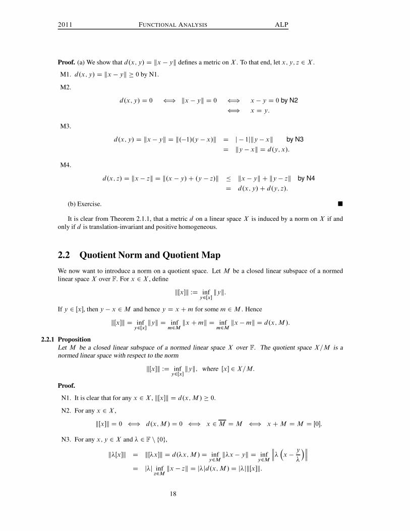
B.a; r / D fx 2 X j kx � ak < r g .Open ball with centre a and radius r /IBŒa; r � D fx 2 X j kx � ak � r g .Closed ball with centre a and radius r /IS.a; r / D fx 2 X j kx � ak D r g .Sphere with centre a and radius r /:

15


1

�1

y

x1�1

k.x; y/k1 D 1

1

�1

y

x1�1

k.x; y/k2 < 1

1

�1

y

x1�1

k.x; y/k1 � 1

Equivalent Norms

2.1.3 Definition

Let k �k and k �k0

be two different norms defined on the same linear space X . We say that k �k is equivalent

to k � k0

if there are positive numbers ˛ and ˇ such that

˛kxk � kxk0� ˇkxk; for all x 2 X:

2.1.4 Example

Let X D Fn. For each x D .x1; x2; : : : ; xn/ 2 X , let

kxk1 DnX

iD1

jxij; kxk2 D

nX

iD1

jxi j2!1

2

; and kxk1 D max1�i�n

jxi j:

We have seen that k � k1; k � k2 and k � k1 are norms on X . We show that these norms are

equivalent.

Equivalence of k � k1 and k � k1: Let x D .x1; x2; : : : ; xn/ 2 X . For each k D 1; 2; : : : ; n,

jxkj �nX

iD1

jxi j ) max1�k�n

jxk j �nX

iD1

jxij ” kxk1 � kxk1:

Also, for k D 1; 2; : : : ; n,

jxk j � max1�k�n

jxk j D kxk1 )nX

iD1

jxij �nX

iD1

kxk1 D nkxk1 ” kxk1 � nkxk1:

Hence, kxk1 � kxk1 � nkxk1.

We now show that k � k2 is equivalent to k � k1. Let x D .x1; x2; : : : ; xn/ 2 X . For each

k D 1; 2; : : : ; n,

jxk j � kxk1 ) jxk j2 � .kxk1/2 )

nX

iD1

jxij2 �nX

iD1

.kxk1/2 D n.kxk1/

2

” kxk2 �p

nkxk1:

16


Also, for each k D 1; 2; : : : ; n,

jxk j �

nX

iD1

jxi j2!1=2

D kxk2 ) max1�k�n

jxk j � kxk2 ” kxk1 � kxk2:

Consequently, kxk1 � kxk2 �p

nkxk1, which proves equivalence of the norms k � k2 and k � k1.

It is, of course, obvious now that all the three norms are equivalent to each other. We shallsee later that all norms on a finite-dimensional normed linear space are equivalent.

2.1.5 Exercise

Let N .X / denote the set of norms on a linear space X . For k � k and k � k0

in N .X /, define a relation' by

k � k ' k � k0

if and only if k � k is equivalent to k � k0:

Show that ' is an equivalence relation on N .X /, i.e., ' is reflexive, symmetric, and transitive.

Open and Closed Sets

2.1.6 Definition

A subset S of a normed linear space .X; k � k/ is open if for each s 2 S there is an � > 0 such that

B.s; �/ � S .

A subset F of a normed linear space .X; k � k/ is closed if its complement X n F is open.

2.1.7 Definition

Let S be a subset of a normed linear space .X; k � k/. We define the closure of S , denoted by S , to be the

intersection of all closed sets containing S .

It is easy to show that S is closed if and only if S D S .

Recall that a metric on a set X is a real-valued function d W X � X ! R which satisfies the following

properties: For all x; y; z 2 X ,

M1. d.x; y/ � 0;

M2. d.x; y/ D 0 ” x D y;

M3. d.x; y/ D d.y; x/;

M4. d.x; z/ � d.x; y/C d.y; z/.

2.1.1 Theorem

(a) If .X; k � k/ is a normed linear space, then

d.x; y/ D kx � yk

defines a metric on X . Such a metric d is said to be induced or generated by the norm k � k. Thus,

every normed linear space is a metric space, and unless otherwise specified, we shall henceforth

regard any normed linear space as a metric space with respect to the metric induced by its norm.

(b) If d is a metric on a linear space X satisfying the properties: For all x; y; z 2 X and for all � 2 F,

.i/ d.x; y/ D d.x C z; y C z/ (Translation Invariance)

.ii/ d.�x; �y/ D j�jd.x; y/ (Absolute Homogeneity);

then

kxk D d.x; 0/

defines a norm on X .

17


Proof. (a) We show that d.x; y/ D kx � yk defines a metric on X . To that end, let x; y; z 2 X .

M1. d.x; y/ D kx � yk � 0 by N1.

M2.

d.x; y/ D 0 ” kx � yk D 0 ” x � y D 0 by N2

” x D y:

M3.

d.x; y/ D kx � yk D k.�1/.y � x/k D j � 1jky � xk by N3

D ky � xk D d.y; x/:

M4.

d.x; z/ D kx � zk D k.x � y/C .y � z/k � kx � yk C ky � zk by N4

D d.x; y/C d.y; z/:

(b) Exercise. �

It is clear from Theorem 2.1.1, that a metric d on a linear space X is induced by a norm on X if and

only if d is translation-invariant and positive homogeneous.

2.2 Quotient Norm and Quotient Map

We now want to introduce a norm on a quotient space. Let M be a closed linear subspace of a normed

linear space X over F. For x 2 X , define

kŒx�k WD infy2Œx�kyk:

If y 2 Œx�, then y � x 2M and hence y D x Cm for some m 2M . Hence

kŒx�k D infy2Œx�kyk D inf

m2Mkx Cmk D inf

m2Mkx �mk D d.x;M /:

2.2.1 Proposition

Let M be a closed linear subspace of a normed linear space X over F. The quotient space X=M is a

normed linear space with respect to the norm

kŒx�k WD infy2Œx�kyk; where Œx� 2 X=M:

Proof.

N1. It is clear that for any x 2 X , kŒx�k D d.x;M / � 0.

N2. For any x 2 X ,

kŒx�k D 0 ” d.x;M / D 0 ” x 2M DM ” x CM DM D Œ0�:

N3. For any x; y 2 X and � 2 F n f0g,

k�Œx�k D kŒ�x�k D d.�x;M /D infy2Mk�x � yk D inf

y2M

��x � y

�

�

D j�j infz2Mkx � zk D j�jd.x;M /D j�jkŒx�k:

18


N4. Let x; y 2 X . Then

kŒx�C Œy�k D kŒx C y�k D d.x C y;M / D infz2Mkx C y � zk

D infz1;z22M

kx C y � .z1 C z2/k

D infz1;z22M

k.x � z1/C .y � z2/k

� infz1;z22M

kx � z1k C ky � z2k

D infz12M

kx � z1k C infz22M

ky � z2k

D d.x;M /C d.y;M / D kŒx�k C kŒy�k:

The norm on X=M as defined in Proposition 2.2.1 is called the quotient norm on X=M .

Let M be a closed subspace of the normed linear space X . The mapping QM from X ! X=M defined

by

QM .x/ D x CM; x 2 X;

is called the quotient map (or natural embedding) of X onto X=M .

2.3 Completeness of Normed Linear Spaces

Now that we have established that every normed linear space is a metric space, we can deploy on a normed

linear space all the machinery that exists for metric spaces.

2.3.1 Definition

Let .xn/1nD1

be a sequence in a normed linear space .X; k � k/.

(a) .xn/1nD1 is said to converge to x if given � > 0 there exists a natural number N D N.�/ such that

kxn � xk < � for all n � N:

Equivalently, .xn/1nD1

converges to x if

limn!1

kxn � xk D 0:

If this is the case, we shall write

xn! x or limn!1

xn D x:

Convergence in the norm is called norm convergence or strong convergence.

(b) .xn/1nD1

is called a Cauchy sequence if given � > 0 there exists a natural number N D N.�/ such

that

kxn � xmk < � for all n;m � N:

Equivalently, .xn/ is Cauchy if

limn;m!1

kxn � xmk D 0:

19


In the following lemma we collect some elementary but fundamental facts about normed linear spaces.

In particular, it implies that the operations of addition and scalar multiplication, as well as the norm and

distance functions, are continuous.

2.3.2 Lemma

Let C be a closed set in a normed linear space .X; k � k/ over F, and let .xn/ be a sequence contained in C

such that limn!1

xn D x 2 X . Then x 2 C .

Proof. Exercise.

2.3.3 Lemma

Let X be a normed linear space and A a nonempty subset of X .

[1] jd.x;A/� d.y;A/j � kx � yk for all x; y 2 X ;

[2] j kxk � kyk j � kx � yk for all x; y 2 X ;

[3] If xn! x, then kxnk ! kxk;

[4] If xn! x and yn ! y, then xn C yn ! x C y;

[5] If xn! x and ˛n! ˛, then ˛nxn ! ˛x;

[6] The closure of a linear subspace in X is again a linear subspace;

[7] Every Cauchy sequence is bounded;

[8] Every convergent sequence is a Cauchy sequence.

Proof. (1). For any a 2 A,

d.x;A/ � kx � ak � kx � yk C ky � ak;

so d.x;A/ � kx�ykCd.y;A/ or d.x;A/�d.y;A/ � kx�yk: Interchanging the roles of x and y gives

the desired result.

(2) follows from (1) by taking A D f0g.(3) is an obvious consequence of (2).

(4), (5) and (8) follow from the triangle inequality and, in the case of (5), the absolute homogeneity.

(6) follows from (4) and (5).

(7). Let .xn/ be a Cauchy sequence in X . Choose n1 so that kxn � xn1k � 1 for all n � n1. By (2),

kxnk � 1C kxn1k for all n � n1. Thus

kxnk � maxf kx1k; kx2k; kx3k; : : : ; kxn1�1k; 1C kxn1kg

for all n.

(8) Let .xn/ be a sequence in X which converges to x 2 X and let � > 0. Then there is a natural

number N such that kxn � xk < �2

for all n � N . For all n;m � N ,

kxn � xmk � kxn � xk C kx � xmk <�

2C �

2D �:

Thus, .xn/ is a Cauchy sequence in X . �

2.3.4 Proposition

Let .X; k�k/ be a normed linear space over F. A Cauchy sequence in X which has a convergent subsequence

is convergent.

20


Proof. Let .xn/ be a Cauchy sequence in X and .xnk/ its subsequence which converges to x 2 X . Then,

for any � > 0, there are positive integers N1 and N2 such that

kxn � xmk <�

2for all n;m � N1

and

kxnk� xk < �

2for all k � N2:

Let N D maxfN1; N2g. If k � N , then since nk � k ,

kxk � xk � kxk � xnkk C kxnk

� xk < �

2C �

2D �:

Hence xn ! x as n!1. �

2.3.5 Definition

A metric space .X; d/ is said to be complete if every Cauchy sequence in X converges in X .

2.3.6 Definition

A normed linear space that is complete with respect to the metric induced by the norm is called a Banach

space.

2.3.1 Theorem

Let .X; k � k/ be a Banach space and let M be a linear subspace of X . Then M is complete if and only if

the M is closed in X .

Proof. Assume that M is complete. We show that M is closed. To that end, let x 2 M . Then there

is a sequence .xn/ in M such that kxn � xk ! 0 as n ! 1. Since .xn/ converges, it is Cauchy.

Completeness of M guarantees the existence of an element y 2M such that kxn � yk ! 0 as n ! 1.

By uniqueness of limits, x D y. Hence x 2M and, consequently, M is closed.

Assume that M is closed. We show that M is complete. Let .xn/ be a Cauchy sequence in M . Then

.xn/ is a Cauchy sequence in X . Since X is complete, there is an element x 2 X such that kxn�xk ! 0

as n ! 1. But then x 2M since M is closed. Hence M is complete. �

2.3.7 Examples

[1] Let 1 � p <1. Then for each positive integer n, .Fn; k � kp/ is a Banach space.

[2] For each positive integer n, .Fn; k � k1/ is a Banach space.

[3] Let 1 � p <1. The sequence space p is a Banach space. Because of the importance ofthis space, we give a detailed proof of its completeness.

The classical sequence space p is complete.

Proof. Let .xn/11 be a Cauchy sequence in p . We shall denote each member of this

sequence by

xn D .xn.1/; xn.2/; : : :/:

Then, given � > 0, there exists an N.�/ D N 2 N such that

kxn � xmkp D 1X

iD1

jxn.i/ � xm.i/jp! 1

p

< � for all n;m � N:

For each fixed index i , we have

jxn.i/ � xm.i/j < � for all n;m � N:

21


That is, for each fixed index i , .xn.i//11 is a Cauchy sequence in F. Since F is complete,

there exists x.i/ 2 F such that

xn.i/! x.i/ as n!1:

Define x D .x.1/; x.2/; : : :/. We show that x 2 p, and xn ! x. To that end, for each k 2 N,

kX

iD1


p

� kxn � xmkp D 1X

iD1


p

< �:

That is,kX

iD1

jxn.i/ � xm.i/jp < �p ; for all k D 1; 2; 3; : : : :

Keep k and n � N fixed and let m!1. Since we are dealing with a finite sum,

kX

iD1

jxn.i/ � x.i/jp � �p :

Now letting k !1, then for all n � N ,

1X

iD1

jxn.i/ � x.i/jp � �p; .2:3:7:1/

which means that xn � x 2 p . Since xn 2 p , we have that x D .x � xn/C xn 2 p . It also

follows from (2.3.7.1) that xn! x as n!1. �

[4] The space `0 of all sequences .xi /11

with only a finite number of nonzero terms is an in-

complete normed linear space. It suffices to show that `0 is not closed in `2 (and hence not

complete). To that end, consider the sequence .xi/11 with terms

x1 D .1; 0; 0; 0; : : :/

x2 D .1;1

2; 0; 0; 0; : : :/

x3 D .1;1

2;

1

22; 0; 0; 0; : : :/

:::

xn D .1;1

2;

1

22; : : : ;

1

2n�1; 0; 0; 0; : : :/

:::

This sequence .xi/11

converges to

x D .1; 1

2;

1

22; : : : ;

1

2n�1;

1

2n;

1

2nC1; : : :/:

Indeed, since x � xn D .0; 0; 0; : : : ; 0; 12n ;

1

2nC1 ; : : :/, it follows that

kxn � xk2 D1X

kDn

1

22k! 0 as n!1:

That is, xn! x as n!1, but x 62 `0: �

22


[5] The space C2Œ�1; 1� of continuous real-valued functions on Œ�1; 1� with the norm

kxk2 D

0@

1Z

�1

x2.t/dt

1A

1=2

is an incomplete normed linear space.

To see this, it suffices to show that there is a Cauchy sequence in C2Œ�1; 1� which converges

to an element which does not belong to C2Œ�1; 1�. Consider the sequence .xn/112 C2Œ�1; 1�

defined by

xn.t/ D

8ˆ<ˆ:

0 if � 1 � t � 0

nt if 0 � t � 1n

1 if 1n� t � 1:

1

y

t0 1

xn.t/

1n�1

We show that .xn/11

is a Cauchy sequence in C2Œ�1; 1�. To that end, for positive integers m

and n such that m > n,

kxn � xmk22 D

1Z

�1

Œxn.t/ � xm.t/�2 dt

D1=mZ

0

Œnt �mt �2 dt C1=nZ

1=m

Œ1 � nt �2 dt

D1=mZ

0

Œm2t2 � 2mnt2 C n2t2� dt C1=nZ

1=m

Œ1 � 2nt C n2t2� dt

D .m2 � 2mnC n2/t3

3

ˇˇ1=m

0

C�

t � nt2 C n2 t3

3

�ˇˇ1=n

1=m

D m2 � 2mnC n2

3m2nD .m� n/2

3m2n! 0 as n;m!1:

Define

x.t/ D�

0 if � 1 � t � 0

1 if 0 < t � 1:

23


Then x 62 C2Œ�1; 1�, and

kxn � xk22 D

1Z

�1

Œxn.t/ � x.t/�2 dt D

1nZ

0

Œnt � 1�2 dt D 1

3n! 0 as n!1:

That is, xn! x as n!1. �

2.4 Series in Normed Linear Spaces

Let .xn/ be a sequence in a normed linear space .X; k � k/. To this sequence we associate another sequence

.sn/ of partial sums, where sn DnX

kD1

xk .

2.4.1 Definition

Let .xn/ be a sequence in a normed linear space .X; k � k/. If the sequence .sn/ of partial sums converges to

s, then we say that the series

1X

kD1

xk converges and that its sum is s. In this case we write

1X

kD1

xk D s.

The series

1X

kD1

xk is said to be absolutely convergent if

1X

kD1

kxkk <1.

We now give a series characterization of completeness in normed linear spaces.

2.4.1 Theorem

A normed linear space .X; k � k/ is a Banach space if and only if every absolutely convergent series in X is

convergent.

Proof. Let X be a Banach space and suppose that

1X

jD1

kxjk <1. We show that the series

1X

jD1

xj converges.

To that end, let � > 0 and for each n 2 N, let sn DnX

jD1

xj . Let K be a positive integer such that

1X

jDK C1

kxjk < �. Then, for all m > n > K, we have

ksm � snk D

mX

1

xj �nX

1

xj

D

mX

nC1

xj

�mX

nC1

kxjk �1X

nC1

kxjk �1X

K C1

kxjk < �:

Hence the sequence .sn/ of partial sums forms a Cauchy sequence in X . Since X is complete, the sequence

.sn/ converges to some element s 2 X . That is, the series

1X

jD1

xj converges.

Conversely, assume that .X; k � k/ is a normed linear space in which every absolutely convergent series

converges. We show that X is complete. Let .xn/ be a Cauchy sequence in X . Then there is an n1 2 N

such that kxn1� xmk < 1

2whenever m > n1. Similarly, there is an n2 2 N with n2 > n1 such that

kxn2� xmk < 1

22 whenever m > n2. Continuing in this way, we get natural numbers n1 < n2 < � � � such

24


that kxnk�xmk < 1

2k whenever m > nk . In particular, we have that for each k 2 N, kxnkC1�xnk

k < 2�k .

For each k 2 N, let yk D xnkC1� xnk

. Then

nX

kD1

kykk DnX

kD1

kxnkC1� xnk

k <nX

kD1

1

2k:

Hence,

1X

kD1

kykk <1. That is, the series

1X

kD1

yk is absolutely convergent, and hence, by our assumption,

the series

1X

kD1

yk is convergent in X . That is, there is an s 2 X such that sj DjX

kD1

yk ! s as j !1. It

follows that

sj DjX

kD1

yk DjX

kD1

ŒxnkC1� xnk

� D xnjC1� xn1

j!1�! s:

Hence xnjC1

j!1�! s C xn1

. Thus, the subsequence�xnk

�of .xn/ converges in X . But if a Cauchy

sequence has a convergent subsequence, then the sequence itself also converges (to the same limit as the

subsequence). It thus follows that the sequence .xn/ also converges in X . Hence X is complete. �

We now apply Theorem 2.4.1 to show that if M is a closed linear subspace of a Banach space X , then

the quotient space X=M , with the quotient norm, is also a Banach space.

2.4.2 Theorem

Let M be a closed linear subspace of a Banach space X . Then the quotient space X=M is a Banach space

when equipped with the quotient norm.

Proof. Let .Œxn�/ be a sequence in X=M such that

1X

jD1

kŒxj �k < 1. For each j 2 N, choose an element

yj 2M such that

kxj � yjk � kŒxj �k C 2�j :

It now follows that

1X

jD1

kxj � yjk < 1, i.e., the series

1X

jD1

.xj � yj / is absolutely convergent in X . Since

X is complete, the series

1X

jD1

.xj � yj / converges to some element z 2 X . We show that the series

1X

jD1

Œxj �

converges to Œz�. Indeed, for each n 2 N,

nX

jD1

Œxj �� Œz�

D

24

nX

jD1

xj

35� Œz�

D

24

nX

jD1

xj � z

35

D infm2M

nX

jD1

xj � z �m

�

nX

jD1

xj � z �nX

jD1

yj

D

nX

jD1

.xj � yj / � z

! 0 as n!1:

25


Hence, every absolutely convergent series in X=M is convergent, and so X=M is complete. �

2.5 Bounded, Totally Bounded, and Compact Subsets of a Normed

Linear Space

2.5.1 Definition

A subset A of a normed linear space .X; k � k/ is bounded if A � BŒx; r � for some x 2 X and r > 0.

It is clear that A is bounded if and only if there is a C > 0 such that kak � C for all a 2 A.

2.5.2 Definition

Let A be a subset of a normed linear space .X; k � k/ and � > 0. A subset A� � X is called an �-net for A

if for each x 2 A there is an element y 2 A� such that kx � yk < �. Simply put, A� � X is an �-net for A

if each element of A is within an � distance to some element of A� .

A subset A of a normed linear space .X; k � k/ is totally bounded (or precompact) if for any � > 0 there

is a finite �-net F� � X for A. That is, there is a finite set F� � X such that

A �[

x2F�

B.x; �/:

The following proposition shows that total boundedness is a stronger property than boundedness.

2.5.3 Proposition

Every totally bounded subset of a normed linear space .X; k � k/ is bounded.

Proof. This follows from the fact that a finite union of bounded sets is also bounded. �

The following example shows that boundedness does not, in general, imply total boundedness.

2.5.4 Example

Let X D `2 and consider B D B.X / D fx 2 X j kxk � 1g, the closed unit ball in X . Clearly, B

is bounded. We show that B is not totally bounded. Consider the elements of B of the form: for

j 2 N, ej D .0; 0; : : : ; 0; 1; 0; : : :/, where 1 occurs in the j -th position. Note that kei � ejk2 Dp

2

for all i ¤ j . Assume that an �-net B� � X existed for 0 < � <p

22

. Then for each j 2 N,

there is an element yj 2 B� such that kej � yjk < �. This says that for each j 2 N, there is an

element yj 2 B� such that yj 2 B.ej ; �/. But the balls B.ej ; �/ are disjoint. Indeed, if i 6D j , andz 2 B.ei ; �/\B.ej ; �/, then by the triangle inequality

p2 D kei � ejk2 � kei � zk C kz � ejk < 2� <

p2;

which is absurd. Since the balls B.ej ; �/ are (at least) countably infinite, there can be no finite

�-net for B.

In our definition of total boundedness of a subset A � X , we required that the finite �-net be a subset

of X . The following proposition suggests that the finite �-net may actually be assumed to be a subset of A

itself.

26


2.5.5 Proposition

A subset A of a normed linear space .X; k � k/ is totally bounded if and only if for any � > 0 there is a finite

set F� � A such that

A �[

x2F�

B.x; �/:


We now give a characterization of total boundedness.

2.5.1 Theorem

A subset K of a normed linear space .X; k � k/ is totally bounded if and only if every sequence in K has a

Cauchy subsequence.

Proof. Assume that K is totally bounded and let .xn/ be an infinite sequence in K. There is a finite set of

points fy11; y12; : : : ; y1r g in K such that

K �r[

jD1

B.y1j ;1

2/:

At least one of the balls B.y1j ;12/; j D 1; 2; : : : ; r , contains an infinite subsequence .xn1/ of .xn/. Again,

there is a finite set fy21; y22; : : : ; y2sg in K such that

K �s[

jD1

B.y2j ;1

22/:

At least one of the balls B.y2j ;1

22 /; j D 1; 2; : : : ; s, contains an infinite subsequence .xn2/ of .xn1/.

Continuing in this way, at the m-th step, we obtain a subsequence .xnm/ of .xn.m�1// which is contained in

a ball of the form B�ymj ;

12m

�.

Claim: The diagonal subsequence .xnn/ of .xn/ is Cauchy. Indeed, if m > n, then both xnn and xmm are

in the ball of radius 2�n. Hence, by the triangle inequality,

kxnn � xmmk < 21�n ! 0 as n ! 1:

Conversely, assume that every sequence in K has a Cauchy subsequence and that K is not totally

bounded. Then, for some � > 0, no finite �-net exists for K. Hence, if x1 2 K, then there is an x2 2 K

such that kx1 � x2k � �. (Otherwise, kx1 � yk < � for all y 2 K and consequently fx1g is a finite �-net

for K, a contradiction.) Similarly, there is an x3 2 K such that

kx1 � x3k � � and kx2 � x3k � �:

Continuing in this way, we obtain a sequence .xn/ in K such that kxn � xmk � � for all m ¤ n. Therefore

.xn/ cannot have a Cauchy subsequence, a contradiction. �

2.5.6 Definition

A normed linear space .X; k � k/ is sequentially compact if every sequence in X has a convergent subse-

quence.

2.5.7 Remark

It can be shown that on a metric space, compactness and sequential compactness are equivalent. Thus, it

follows, that on a normed linear space, we can use these terms interchangeably.

27


2.5.2 Theorem

A subset of a normed linear space is sequentially compact if and only if it is totally bounded and complete.

Proof. Let K be a sequentially compact subset of a normed linear space .X; k � k/. We show that K is

totally bounded. To that end, let .xn/ be a sequence in K. By sequential compactness of K, .xn/ has a

subsequence .xnk/ which converges in K. Since every convergent sequence is Cauchy, the subsequence

.xnk/ of .xn/ is Cauchy. Therefore, by Theorem 2.5.1, K is totally bounded.

Next, we show that K is complete. Let .xn/ be a Cauchy sequence in K. By sequential compactness

of K, .xn/ has a subsequence .xnk/ which converges in K. But if a subsequence of a Cauchy sequence

converges, so does the full sequence. Hence .xn/ converges in K and so K is complete.

Conversely, assume that K is a totally bounded and complete subset of a normed linear space .X; k � k/.We show that K is sequentially compact. Let .xn/ be a sequence in K. By Theorem 2.5.1, .xn/ has a Cauchy

subsequence .xnk/. Since K is complete, .xnk

/ converges in K. Hence K is sequentially compact. �

2.5.8 Corollary

A subset of a Banach space is sequentially compact if and only if it is totally bounded and closed.


2.5.9 Corollary

A sequentially compact subset of a normed linear space is closed and bounded.


We shall see that in finite-dimensional spaces the converse of Corollary 2.5.9 also holds.

2.5.10 Corollary

A closed subset F of a sequentially compact normed linear space .X; k � k/ is sequentially compact.


2.6 Finite Dimensional Normed Linear Spaces

The theory for finite-dimensional normed linear spaces turns out to be much simpler than that of their

infinite-dimensional counterparts. In this section we highlight some of the special aspects of finite-dimensional

normed linear spaces.

The following Lemma is crucial in the analysis of finite-dimensional normed linear spaces.

2.6.1 Lemma

Let .X; k � k/ be a finite-dimensional normed linear space with basis fx1; x2; : : : ; xng. Then there is a

constant m > 0 such that for every choice of scalars ˛1; ˛2; : : : ; ˛n, we have

m

nX

jD1

j j j �

nX

jD1

j xj

:

28


Proof. If

nX

jD1

j j j D 0, then j D 0 for all j D 1; 2; : : : ; n and the inequality holds for any m > 0.

Assume that

nX

jD1

j j j ¤ 0. We shall prove the result for a set of scalars f˛1; ˛2; : : : ; ˛ng that satisfy the

condition

nX

jD1

j j j D 1. Let

A D f.˛1; ˛2; : : : ; ˛n/ 2 Fn jnX

jD1

j j j D 1g:

Since A is a closed and bounded subset of Fn, it is compact. Define f W A! R by

f .˛1; ˛2; : : : ; ˛n/ D

nX

jD1

j xj

:

Since for any .˛1; ˛2; : : : ; ˛n/ and .ˇ1; ˇ2; : : : ; ˇn/ in A

jf .˛1; ˛2; : : : ; ˛n/ � f .ˇ1; ˇ2; : : : ; ˇn/j D

ˇˇˇ

nX

jD1

j xj

�

nX

jD1

j xj

ˇˇˇ

�

nX

jD1

j xj �nX

jD1

j xj

D

nX

jD1

. j � j /xj

�

nX

jD1

j j � j jkxjk

� max1�j�n

kxjknX

jD1

j j � j j;

f is continuous on A. Since f is a continuous function on a compact set A, it attains its minimum on A,

i.e., there is an element .�1; �2; : : : ; �n/ 2 A such that

f .�1; �2; : : : ; �n/ D infff .˛1; ˛2; : : : ; ˛n/ j .˛1; ˛2; : : : ; ˛n/ 2 Ag:

Let m D f .�1; �2; : : : ; �n/. Since f � 0, it follows that m � 0. If m D 0, then

nX

jD1

�j xj

D 0 )

nX

jD1

�j xj D 0:

Since the set fx1; x2; : : : ; xng is linearly independent, �j D 0 for all j D 1; 2; : : : ; n. This is a

contradiction since .�1; �2; : : : ; �n/ 2 A. Hence m > 0 and consequently for all .˛1; ˛2; : : : ; ˛n/ 2 A,

0 < m � f .˛1; ˛2; : : : ; ˛n/ ” m

nX

jD1

j j j �

nX

jD1

j xj

:

Now, let f˛1; ˛2; : : : ; ˛ng be any collection of scalars and set ˇ DnX

jD1

j j j. If ˇ D 0, then the

29


inequality holds vacuously. If ˇ > 0, then

�˛1

ˇ;˛2

ˇ; : : : ;

˛n

ˇ

�2 A and consequently

nX

jD1

j xj

D

nX

jD1

j

ˇxj

ˇ D f

�˛1

ˇ;˛2

ˇ; : : : ;

˛n

ˇ

�ˇ � mˇ D m

nX

jD1

j j j:

That is, m

nX

jD1

j j j �

nX

jD1

j xj

. �

2.6.1 Theorem

Let X be a finite-dimensional normed linear space over F. Then all norms on X are equivalent.

Proof. Let fx1; x2; : : : ; xng be a basis for X and k � k0 and k � k be any two norms on X . For any x 2 X

there is a set of scalars f˛1; ˛2; : : : ; ˛ng such that x DnX

jD1

jxj . By Lemma 2.6.1, there is an m > 0 such

that

m

nX

jD1

j j j �

nX

jD1

jxj

D kxk:

By the triangle inequality

kxk0 �nX

jD1

j j jkxjk0 �M

nX

jD1

j j j;

where M D max1�j�n

kxjk0. Hence

kxk0 �M

�1

mkxk

�)

m

Mkxk0 � kxk ” ˛kxk0 � kxk where ˛ D

m

M:

Interchanging the roles of the norms k � k0 and k � k, we similarly get a constant ˇ such that kxk � ˇkxk0.

Hence, ˛kxk0 � kxk � ˇkxk0 for some constants ˛ and ˇ. �

2.6.2 Theorem

Every finite-dimensional normed linear space .X; k � k/ is complete.

Proof. Let fx1; x2; : : : ; xng be a basis for X and let .zk / be a Cauchy sequence in X . Then, given any

� > 0, there is a natural number N such that

kzk � z`k < � for all k; ` > N:

Also, for each k 2 N, zk DnX

jD1

˛kj xj . By Lemma 2.6.1, there is an m > 0 such that

m

nX

jD1

j˛kj � ˛`j j � kzk � z`k:

Hence, for all k; ` > N and all j D 1; 2; : : : ; n,

j˛kj � ˛`j j �1

mkzk � z`k <

�

m:

30


That is, for each j D 1; 2; : : : ; n, .˛kj /k is a Cauchy sequence of numbers. Since F is complete, ˛kj ! j

as k !1 for each j D 1; 2; : : : ; n. Define z DnX

jD1

jxj . Then z 2 X and

kzk � zk D

nX

jD1

˛kj xj �nX

jD1

jxj

D

nX

jD1

.˛kj � j /xj

�

nX

jD1

j˛kj � j jkxjk ! 0

as k !1. That is, the sequence .zk / converges to z 2 X . hence X is complete. �

2.6.2 Corollary

Every finite-dimensional normed linear space X is closed.


2.6.3 Theorem

In a finite-dimensional normed linear space .X; k � k/, a subset K � X is sequentially compact if and only

if it is closed and bounded.

Proof. We have seen (Corollary 2.5.9), that a compact subset of a normed linear space is closed and

bounded.

Conversely, assume that a subset K � X is closed and bounded. We show that K is compact. Let

fx1; x2; : : : ; xng be a basis for X and let .zk / be any sequence in K. Then for each k 2 N, zk DnX

jD1

˛kjxj .

Since K is bounded, there is a positive constant M such that kzkk � M for all k 2 N. By Lemma 2.6.1,

there is an m > 0 such that

m

nX

jD1

j˛kj j �

nX

jD1

˛kj xj

D kzkk �M:

It now follows that j˛kj j � Mm

for each j D 1; 2; : : : ; n, and for all k 2 N. That is, for each fixed j D1; 2; : : : ; n, the sequence .˛kj /k of numbers is bounded. Hence the sequence .˛kj /k has a subsequence

.˛kr j / which converges to j for j D 1; 2; : : : ; n. Setting z DnX

jD1

jxj , we have that

kzkr� zk D

nX

jD1

˛kr jxj �nX

jD1

j xj

�

nX

jD1

j˛kr j � j jkxjk ! 0 as r !1:

That is, zkr! z as r !1. Since K is closed, z 2 K. Hence K is compact. �

2.6.3 Lemma

(Riesz’s Lemma). Let M be a closed proper linear subspace of a normed linear space .X; k � k/. Then for

each 0 < � < 1, there is an element z 2 X such that kzk D 1 and

ky � zk > 1 � � for all y 2M:

Proof. Choose x 2 X nM and define

d D d.x;M / D infm2M

kx �mk:

31


Since M is closed, d > 0. By definition of infimum, there is a m 2M such that

d � kx �mk < d C �d D d.1C �/:

Take z D ��

m� x

km� xk

�. Then kzk D 1 and for any y 2M ,

ky � zk D y C

�m� x

km� xk

� Dky.km � xk/Cm� xk

km� xk

� d

km� xk >d

d.1C �/ D1

1C � D 1 � �

1C � > 1 � �:

We now give a topological characterization of the algebraic concept of finite dimensionality.

2.6.4 Theorem

A normed linear space .X; k � k/ is finite-dimensional if and only its closed unit ball B.X / D fx 2X j kxk � 1g is compact.

Proof. Assume that .X; k � k/ is finite-dimensional normed linear space. Since the ball B.X / is closed and

bounded, it is compact.

Assume that the closed unit ball B.X / D fx 2 X j kxk � 1g is compact. Then B.X / is totally

bounded. Hence there is a finite 12

-net fx1; x2; : : : ; xng in B.X /. Let M Dlinfx1; x2; : : : ; xng. Then

M is a finite-dimensional linear subspace of X and hence closed.

Claim: M D X . If M is a proper subspace of X , then, by Riesz’s Lemma there is an element x0 2 B.X /

such that d.x0;M / > 12

. In particular, kx0 � xkk > 12

for all k D 1; 2; : : : ; n: However this contradicts

the fact that fx1; x2; : : : ; xng is a 12

-net in B.X /. Hence M D X and, consequently, X is finite-

dimensional. �

We now give another argument to show that boundedness does not imply total boundedness. Let X D `2

and B.X / D fx 2 X j kxk2 � 1g. It is obvious that B.X / is bounded. We show that B.X / is not totally

bounded. Since X is complete and B.X / is a closed subset of X , B.X / is complete. If B.X / were totally

bounded, then B.X / would, according to Theorem 2.26, be compact. By Theorem 2.6.4, X would be

finite-dimensional. But this is false since X is infinite-dimensional.

2.7 Separable Spaces and Schauder Bases

2.7.1 Definition

(a) A subset S of a normed linear space .X; k � k/ is said to be dense in X if S D X ; i.e., for each x 2 X

and � > 0, there is a y 2 S such that kx � yk < �.

(b) A normed linear space .X; k � k/ is said to be separable if it contains a countable dense subset.

2.7.2 Examples

[1] The real line R is separable since the set Q of rational numbers is a countable dense subset

of R.

[2] The complex plane C is separable since the set of all complex numbers with rational real

and imaginary parts is a countable dense subset of C.

[3] The sequence space p, where 1 � p < 1, is separable. Take M to be the set of all

sequences with rational entries such that all but a finite number of the entries are zero. (If

32


the entries are complex, take for M the set of finitely nonzero sequences with rational realand imaginary parts.) It is clear that M is countable. We show that M is dense in p . Let

� > 0 and x D .xn/ 2 p. Then there is an N such that

1X

kDN C1

jxk jp <�

2:

Now, for each 1 � k � N , there is a rational number qk such that jxk � qk jp < �2N

. Set

q D .q1; q2; : : : ; qN; 0; 0; : : :/. Then q 2M and

kx � qkpp D

NX

kD1

jxk � qk jp C1X

kDN C1

jxk jp < �:

Hence M is dense in p.

[4] The sequence space `1, with the supremum norm, is not separable. To see this, considerthe set M of elements x D .xn/, in which xn is either 0 or 1. This set is uncountable since

we may consider each element of M as a binary representation of a number in the interval

Œ0; 1�. Hence there are uncountably many sequences of zeroes and ones. For any two

distinct elements x; y 2 M , kx � yk1 D 1. Let each of the elements of M be a centre of

a ball of radius 14. Then we get uncountably many nonintersecting balls. If A is any dense

subset of `1, then each of these balls contains a point of A. Hence A cannot be countable

and, consequently, `1 is not separable.

2.7.1 Theorem

A normed linear space .X; k � k/ is separable if and only if it contains a countable set B such that lin.B/ DX .

Proof. Assume that X is separable and let A be a countable dense subset of X . Since the linear hull of A,

lin.A/, contains A and A is dense in X , we have that lin.A/ is dense in X , that is, lin.A/ D X .

Conversely, assume that X contains a countable set B such that lin.B/ D X . Let B D fxn j n 2 Ng.Assume first that D R, and put

C D

8<:

nX

jD1

�jxj j �j 2 Q; j D 1; 2; : : : ; n; n 2 N

9=; :

We first show that C is a countable subset of X . The set Q � B is countable and consequently, the family

F of all finite subsets of Q � B is also countable. The mapping

f.�1; x1/; .�2; x2/; : : : ; .�n; xn/g 7!nX

jD1

�jxj

maps F onto C . Hence C is countable.

Next, we show that C is dense in X . Let x 2 X and � > 0. Since lin.B/ D X , we can find an n 2 N,

points x1; x2; : : : ; xn 2 B and �1; �2; : : : ; �n 2 F such that

x �

nX

jD1

�jxj

<�

2:

33


Since Q is dense in R, for each �i 2 R, we can find a �i 2 Q such that

j�i � �i j <�

2n.1C kxik/for all i D 1; 2; : : : ; n:

Hence, x �

nX

jD1

�jxj

�

x �

nX

jD1

�jxj

C

nX

jD1

�jxj �nX

jD1

�jxj

<�

2C

nX

jD1

j�j � �j jkxjk

<�

2C

nX

jD1

�kxjk2n.1C kxjk/

<�

2C �

2D �:

This shows that C is dense in X .

If F D C, the set C is that of finite linear combinations with coefficients being those complex numbers with

rational real and imaginary parts.

We now give another argument based on Theorem 2.7.1 to show that the sequence space p , where

1 � p <1, is separable. Let en D .ınm/m2N, where

ınm D�

1 if n D m

0 otherwise:

Clearly, en 2 p . Let � > 0 and x D .xn/ 2 p . Then there is a natural number N such that

1X

kDnC1

jxkjp < �p for all n � N:

Now, if n � N , then x �

nX

jD1

xjej

p

D

0@

1X

kDnC1

jxk jp1A

1=p

< �:

Hence lin.fen j n 2 Ng/ D p . Of course, the set fen j n 2 Ng is countable.

2.7.3 Definition

A sequence .bn/ in a Banach space .X; k � k/ is called a Schauder basis if for any x 2 X , there is a unique

sequence .˛n/ of scalars such that

limn!1

x �

nX

jD1

jbj

D 0:

In this case we write x D1X

jD1

jbj :

2.7.4 Remark

It is clear from Definition 2.7.3 that .bn/ is a Schauder basis if and only if X D linfbn j n 2 Ng and

every x 2 X has a unique expansion x D1X

jD1

jbj :

Uniqueness of this expansion clearly implies that the set fbn j n 2 Ng is linearly independent.

34


2.7.5 Examples

[1] For 1 � p <1, the sequence .en/, where en D .ınm/m2N, is a Schauder basis for p .

[2] .en/ is a Schauder basis for c0.

[3] .en/[ feg, where e D .1; 1; 1; : : :/ (the constant 1 sequence), is a Schauder basis for c.

[4] `1 has no Schauder basis.

2.7.6 Proposition

If a Banach space .X; k � k/ has a Schauder basis, then it is separable.

Proof. Let .bn/ be a Schauder basis for X . Then fbn j n 2 Ng is countable and

lin.fbn j n 2 Ng/ D X . �

Schauder bases have been constructed for most of the well-known Banach spaces. Schauder conjectured

that every separable Banach space has a Schauder basis. This conjecture, known as the Basis Problem,

remained unresolved for a long time until Per Enflo in 1973 answered it in the negative. He constructed a

separable reflexive Banach space with no basis.

2.7.7 Exercise

[1] Let X be a normed linear space over F. Show that X is finite-dimensional if and only if everybounded sequence in X has a convergent subsequence.

[2] Complete the proof of Theorem 2.1.1.

[3] Prove Lemma 2.3.2.

[4] Prove the claims made in [1] and [2] of Example 2.3.7.

[5] Prove Theorem 2.5.5.

[6] Prove Corollary 2.5.8.




[10] Is .CŒa; b�; k � k1/ complete? What about .CŒa; b�; k � k1/? Fully justify both answers.

35

Chapter 3

Hilbert Spaces

3.1 Introduction

In this chapter we introduce an inner product which is an abstract version of the dot product in elementary

vector algebra. Recall that if x D .x1; x2; x3/ and y D .y1; y2; y3/ are any two vectors in R3, then the

dot product of x and y is x � y D x1y1 C x2y2 C x3y3. Also, the length of the vector x is kxk Dqx2

1 C x22 C x2

3 Dp

x � x.

It turns out that Hilbert spaces are a natural generalization of finite-dimensional Euclidean spaces.

Hilbert spaces arise naturally and frequently in mathematics, physics, and engineering, typically as infinite-

dimensional function spaces.

3.1.1 Definition

Let X be a linear space over a field F. An inner product on X is a scalar-valued function h�; �i W X�X ! F

such that for all x; y; z 2 X and for all ˛; ˇ 2 F, we have

IP1. hx; xi � 0;

IP2. hx; xi D 0 ” x D 0;

IP3. hx; yi D hy; xi (The bar denotes complex conjugation.);

IP4. h˛x; yi D ˛hx; yi;

IP5. hx C y; zi D hx; zi C hy; zi.

An inner product space .X; h�; �i/ is a linear space X together with an inner h�; �i product defined on it. An

inner product space is also called pre-Hilbert space.

3.1.2 Examples

Examples of inner product spaces.

[1] Fix a positive integer n. Let X D Fn. For x D .x1; x2; : : : ; xn/ and y D .y1; y2; : : : ; yn/ in X ,

define

hx; yi DnX

iD1

xiyi :

Since this is a finite sum, h�; �i is well-defined. It is easy to show that .X; h�; �i/ is an inner

product space. The space Rn (resp. Cn) with this inner product is called the Euclidean

n-space (resp. unitary n-space) and will be denoted by `2.n/.

36


[2] Let X D `0, the linear space of finitely non-zero sequences of real or complex numbers. Forx D .x1; x2; : : :/ and y D .y1; y2; : : :/ in X , define

hx; yi D1X

iD1

xiyi :

Since this is essentially a finite sum, h�; �i is well-defined. It is easy to show that .X; h�; �i/ is

an inner product space.

[3] Let X D `2, the space of all sequences x D .x1; x2; : : :/ of real or complex numbers with1X

1

jxi j2 <1. For x D .x1; x2; : : :/ and y D .y1; y2; : : :/ in X , define

hx; yi D1X

iD1

xiyi :

In order to show that h�; �i is well-defined we first observe that if a and b are real numbers,

then

0 � .a � b/2; whence ab � 1

2.a2 C b2/:

Using this fact, we have that

jxiyi j D jxi jjyi j �1

2

�jxij2 C jyi j2

�)

1X

iD1

jxiyi j �1

2

1X

iD1

jxij2 C1X

iD1

jyi j2!<1:

Hence, h�; �i is well-defined (i.e., the series converges).

[4] Let X D CŒa; b�, the space of all continuous complex-valued functions on Œa; b�. For x; y 2 X ,

define

hx; yi DbZ

a

x.t/y.t/ dt:

We shall denote by C2Œa; b� the linear space CŒa; b� equipped with this inner product.

[5] Let X D L.Cn/ be the linear space of all n � n complex matrices. For A 2 L.Cn/, let

�.A/ DnX

iD1

.A/ii be the trace of A. For A;B 2 L.Cn/, define

hA;Bi D �.B�A/; where B� denotes conjugate transpose of matrix B:

Show that .L.Cn/; h�; �i/ is an inner product space.

It should be mentioned that we could consider real Hilbert spaces but there are powerful methods that

can be applied by using the more general complex Hilbert spaces.

3.1.1 Theorem

(Cauchy-Bunyakowsky-Schwarz Inequality). Let .X; h�; �i/ be an inner product space over a field F.

Then for all x; y 2 X ,

jhx; yij �phx; xi

phy; yi:

Moreover, given any x; y 2 X , the equality

jhx; yij Dphx; xi

phy; yi

holds if and only if x and y are linearly dependent.

37


Proof. If x D 0 or y D 0, then the result holds vacuously. Assume that x 6D 0 and y 6D 0. For any ˛ 2 F,

we have

0 � hx � ˛y; x � ˛yi D hx; xi � ˛hy; xi � ˛hx; yi C ˛˛hy; yiD hx; xi � ˛hx; yi � ˛Œhy; xi � ˛hy; yi�:

Now choosing ˛ D hx; yihy; yi

, we have

0 � hx; xi � hy; xihx; yihy; yi D hx; xi � jhx; yij2

hy; yi ;

whence

jhx; yij �phx; xi

phy; yi:

Assume that jhx; yij Dphx; xi

phy; yi. We show that x and y are linearly dependent. If x D 0 or

y D 0, then x and y are obviously linearly dependent. We therefore assume that x 6D 0 and y 6D 0. Then

hy; yi 6D 0. With ˛ D hx; yihy; yi , we have that

hx � ˛y; x � ˛yi D hx; xi �jhx; yij2hy; yi D 0:

That is,

hx � ˛y; x � ˛yi D 0; ) x D ˛y:

That is, x and y are linearly dependent.

Conversely, assume that x and y are linearly dependent. Without loss of generality, x D �y for some

� 2 F. Then

jhx; yij D jh�y; yij D j�jjhy; yij D j�jhy; yi

D j�jphy; yi

phy; yi D

qj�j2hy; yi

phy; yi D

ph�y�yi

phy; yi

Dphx; xi

phy; yi: �

3.1.2 Theorem

Let .X; h�; �i/ be an inner product space over a field F. For each x 2 X , define

kxk WDphx; xi: .3:1:2:1/

Then k � k defines a norm on X . That is, .X; k � k/ is a normed linear space over F.

Proof. Let x; y 2 X and � 2 F. Then

N1. kxk Dphx; xi � 0;

N2. kxk D 0 ”phx; xi D 0 ” hx; xi D 0 ” x D 0; by IP2.

N3. k�xk Dph�x�xi D

pj�j2hx; xi D j�j

phx; xi D j�jkxk.

N4.

38


kx C yk2 D hx C y; x C yi D hx; xi C hx; yi C hy; xi C hy; yiD hx; xi C hx; yi C hx; yi C hy; yiD kxk2 C 2Rehx; yi C kyk2 � kxk2 C 2jhx; yij C kyk2

� kxk2C 2phx; xi

phy; yi C kyk2 (by Theorem 3.1.1)

D kxk2 C 2kxkkyk C kyk2 D .kxk C kyk/2:Taking the positive square root both sides yields

kx C yk � kxk C kyk: �

In view of (3.1.2.1), the Cauchy-Bunyakowsky-Schwarz Inequality now becomes

jhx; yij � kxkkyk:

Any inner product space can thus be made into a normed linear space in a natural way: by defining the norm

as in (3.1.2.1). The norm advertised in (3.1.2.1) is called the inner product norm or a norm induced or

generated by the inner product.

A natural question arises: Is every normed linear space an inner product space? If the answer is NO,

how then does one recognise among all normed linear spaces those that are inner product spaces in disguise,

i.e., those whose norms are induced by an inner product?

These questions will be examined later.

3.1.3 Theorem

(Polarization Identity). Let .X; h�; �i/ be an inner product space over a field F. Then for all x; y 2 X ,

hx; yi D kx C yk2

4� kx � yk2

4if F D R; and

hx; yi D kx C yk2

4� kx � yk2

4C i

�kxCyik2

4� kx � yik2

4

�if F D C:

Proof. Assume that F D R. Then

kx C yk2 � kx � yk2 D hx C y; x C yi � hx � y; x � yiD hx; xi C hx; yi C hy; xi C hy; yi � hx; xi C hx; yi C hy; xi � hy; yiD 4hx; yi; since hx; yi D hy; xi:

The case when F D C is proved analogously and is left as an exercise. �

3.1.4 Theorem

(Parallelogram Identity). Let .X; h�; �i/ be an inner product space over a field F. Then for all x; y 2 X ,

kx � yk2 C kx C yk2 D 2kxk2C 2kyk2: .3:1:4:1/

Proof.

kx � yk2 Ckx C yk2 D hx � y; x � yi C hx C y; x C yiD hx; xi � hx; yi � hy; xi C hy; yi C hx; xi C hx; yi C hy; xi C hy; yiD 2kxk2C 2kyk2: �

The geometric interpretation of the Parallelogram Identity is evident: the sum of the squares of the

lengths of the diagonals of a parallelogram is equal to the sum of the squares of the lengths of the four

39


sides.

x

y

The following theorem asserts that the Parallelogram Identity (Theorem 3.1.4) distinguishes inner prod-

uct spaces among all normed linear spaces. It also answers the question posed after Theorem 3.1.2. That is,

a normed linear space is an inner product space if and only if its norm satisfies the Parallelogram Identity.

3.1.5 Theorem

A normed linear space X over a field F is an inner product space if and only if the Parallelogram Identity

kx � yk2 C kx C yk2 D 2kxk2C 2kyk2 .PI /

holds for all x; y 2 X .

Proof. “)”. We have already shown (Theorem 3.1.4) that if X is an inner product space, then the parallel-

ogram identity (PI) holds in X .

“(”. Let X be a normed linear space in which the parallelogram identity (PI) holds. We shall only

consider the case F D R. The polarization identity (Theorem 3.1.3) gives us a hint as to how we should

define an inner product: For all x; y 2 X , define

hx; yi D

x C y

2

2

� x � y

2

2

:

We claim that h�; �i is an inner product on X .

IP1. hx; xi D

x C x

2

2

� x � x

2

2

D kxk2 � 0.

IP2. hx; xi D 0 ” kxk2 D 0 ” x D 0.

IP3. hx; yi D

x C y

2

2

� x � y

2

2

D

y C x

2

2

� y � x

2

2

D hy; xi D hy; xi since F D R.

IP5. Replace x by uC v and y by w C v in the parallelogram identity:

kuC w C 2vk2C ku �wk2 D 2kuC vk2 C 2kw C vk2: .3:1:5:1/

Replace x by u � v and y by w � v in the parallelogram identity:

kuC w � 2vk2 C ku� wk2 D 2ku � vk2 C 2kw � vk2: .3:1:5:2/

Subtract (3.1.5.2) from (3.1.5.1):

kuC w C 2vk2 � kuC w � 2vk2 D 2hkuC vk2 � ku � vk2 C kv C wk2 � kv �wk2

i:

40


Use the definition of h�; �i,

4huC w; 2vi D 8Œhu; vi C hw; vi� ) 1

2huC w; 2vi D hu; vi C hw; vi: .3:1:5:3/

Take w D 0:1

2hu; 2vi D hu; vi: .3:1:5:4/

Now replace u by x C y and v by z in (3.1.5.4) and use (3.1.5.3) to get

hx C y; zi D 1

2hx C y; 2zi D hx; zi C hy; zi:

IP4. We show that h�x; yi D �hx; yi for all � 2 R and all x; y 2 X . If � D n is a nonzero integer, then

using IP5,

hnx; yi D nhx; yi ) nDxn; yEDDnx

n; yED hx; yi:

That is, Dxn; yED 1

nhx; yi:

If � is a rational number, � D pq

, say. Then

�p

qx; y

�D p

�x

q; y

�D p

qhx; yi:

If � 2 R, then there is a sequence .rk / of rational numbers such that rk ! � as k ! 1. Using

continuity of the norm, we have that

h�x; yi D h limk!1

rkx; yi D 1

4

limk!1

rkx C y

2

� 1

4

limk!1

rkx � y

2

D 1

4lim

k!1krkx C yk2 � 1

4lim

k!1krkx � yk2

D limk!1

rkx C y

2

2

� rkx � y

2

2!

D limk!1hrkx; yi

D limk!1

rkhx; yi D �hx; yi:

Thus, h�x; yi D �hx; yi for all � 2 R and all x; y 2 X . �

3.1.3 Corollary

Let .X; k � k/ be a normed linear space over a field F. If every two-dimensional linear subspace of X is an

inner product space over F, then X is an inner product space.

3.1.4 Examples

[1] Let X D p ; for p 6D 2. Then X is not an inner product space. We show that the norm

on p ; p 6D 2 does not satisfy the parallelogram identity. Take x D .1; 1; 0; 0; : : :/ and

y D .1;�1; 0; 0; : : :/ in p. Then

kxk D 21p D kyk and kx C yk D 2 D kx � yk:

Thus,

kx C yk2 C kx � yk2 D 8 6D 2kxk2C 2kyk2 D 4 � 22p :

41


[2] The normed linear space X D CŒa; b�, with the supremum norm k �k1 is not an inner productspace. We show that the norm

kxk1 D maxa�t�b

jx.t/j

does not satisfy the parallelogram identity. To that end, take

x.t/ D 1 and y.t/ D t � a

b � a:

Since

x.t/C y.t/ D 1C t � a

b � aand x.t/ � y.t/ D 1 � t � a

b � a;

we have thatkxk D 1 D kyk; and kx C yk D 2; kx � yk D 1:

Thus,

kx C yk2 C kx � yk2 D 5 6D 2kxk2C 2kyk2 D 4:

3.2 Completeness of Inner Product Spaces

The mathematical concept of a Hilbert space, named after David Hilbert, generalizes the notion of Euclidean

space. Hilbert spaces, as the following definition states, are inner product spaces which in addition are

required to be complete, a property that stipulates the existence of enough limits in the space to allow the

techniques of calculus to be used.

The earliest Hilbert spaces were studied from this more abstract point of view in the first decade of

the 20th century by David Hilbert, Erhard Schmidt, and Frigyes Riesz. They are indispensable tools in

the theories of partial differential equations, quantum mechanics, Fourier analysis which includes applica-

tions to signal processing, and ergodic theory which forms the mathematical underpinning of the study of

thermodynamics.

3.2.1 Definition

Let .X; h�; �i/ be an inner product space. If X is complete with respect to the norm induced by the inner

product h�; �i, then we say that X is a Hilbert space.

3.2.2 Examples

[1] The classical space `2 is a Hilbert space.

[2] `0 is an incomplete inner product space.

[3] The space CŒ�1; 1� is an incomplete inner product space.

3.3 Orthogonality

3.3.1 Definition

Two elements x and y in an inner product space .X; h�; �i/ are said to be orthogonal, denoted by x ? y, if

hx; yi D 0:

The set M � X is called orthogonal if it consists of non-zero pairwise orthogonal elements.

If M is a subset of X such that hx;mi D 0 for all m 2M , then we say that x is orthogonal to M and write

x ?M . We shall denote by

M ? D fx 2 X W hx;mi D 0 8 m 2M g

42


the set of all elements in X that are orthogonal to M . The set M ? is called the orthogonal complement

of M .

3.3.2 Proposition

Let M and N be subsets of an inner product space .X; h�; �i/. Then

[1] f0g? D X and X ? D f0g;

[2] M ? is a closed linear subspace of X ;

[3] M � .M ?/? DM ??;

[4] If M is a linear subspace, then M \M ? D f0g;

[5] If M � N , then N ? �M ?;

[6] M ? D .linM /? D .linM /?.

Proof.

[1] Exercise.

[2] Let x; y 2M ?, and ˛; ˇ 2 F. Then for each z 2M ,

h˛x C ˇy; zi D ˛hx; zi C ˇhy; zi D 0:

Hence, ˛x C ˇy 2M ?. That is, M ? is a subspace of X . To show that M ? is closed, let x 2M ?.

Then there exists a sequence .xn/ in M ? such that xn! x as n!1. Thus, for all y 2M ,

hx; yi D limnhxn; yi D 0;

whence x 2M ?.

[3] Exercise.

[4] Exercise.

[5] Let x 2 N ?. Then hx; yi D 0 for all y 2 N . In particular, hx; yi D 0 for all y 2M since M � N .

Thus, x 2M ?.

[6] Since M � linM � linM , we have, by [5], that .linM /? � .linM /? � M ?. It remains to show

that M ? � .linM /?. To that end, let x 2 M ?. Then hx; yi D 0 for all y 2 M , and consequently

hx; yi D 0 for all y 2 linM . If z 2 linM , then there exists a sequence .zn/ in linM such that zn ! z

as n!1. Thus,

hx; zi D limnhx; zni D 0;

whence x 2 .linM /?. �

3.3.3 Examples

Let X D R3. The vectors .�3; 0; 2/ and .4; 1; 6/ are orthogonal since

h.�3; 0; 2/; .4; 1; 6/i D .�3/.4/ C 0.1/C .2/.6/ D 0: �

43


If M D `0, the linear subspace of `2 consisting of all scalar sequences .xi/11 with only a finite

number of nonzero terms, then M ? D f0g. Indeed, suppose that y D .yi /1iD1 2M ?. Let

ıij D

8<:

1 if i D j

0 if i 6D j:

and en D .ınj /1n;jD1

. Then en 2M for each n 2 N, and hence,

0 D hy; eii D1X

jD1

yjıij D yi for all i D 1; 2; : : : :

That is, y D 0, whence M ? D f0g.

3.3.1 Theorem

(Pythagoras). Let .X; h�; �i/ be an inner product space over a field F and let x; y 2 X .

[1] If F D R, then x ? y if and only if

kx C yk2 D kxk2C kyk2:

[2] If F D C, then x ? y if and only if

kx C yk2 D kxk2C kyk2 and kx C iyk2 D kxk2C kyk2:

Proof. [1] “)”. If x ? y, then

kx C yk2 D hx C y; x C yi D hx; xi C 2hx; yi C hy; yi D kxk2C kyk2:

“(”. Suppose that kx C yk2 D kxk2C kyk2: Then

hx C y; x C yi D hx; xiC hy; yi) hx; xi C 2hx; yi C hy; yi D hx; xiC hy; yi

) 2hx; yi D 0 ) hx; yi D 0:

[2] “)”. Assume that x ? y. Then

kx C yik2 D hx C yi ; x C yi i D hx; xiC hx; yii C hyi ; xi C hyi ; yiiD hx; xi � ihx; yi C ihy; xi C hy; yi D kxk2C kyk2:

“(”. Assume that kx C yk2 D kxk2C kyk2 and kx C iyk2 D kxk2C kyk2: Then

hx C y; x C yi D hx; xiC hy; yi) hx; xi C hx; yi C hy; xi C hy; yi D hx; xiC hy; yi

) hx; yi C hy; xi D 0 ) 2Rehx; yi D 0 ) Rehx; yi D 0:

Also,

hx C yi ; x C yii D hx; xiC hy; yi) hx; xi � ihx; yi C ihy; xi C hy; yi D hx; xi C hy; yi) �ihx; yi C ihy; xi D 0

) �i Œhx; yi � hy; xi�D 0

) �ihhx; yi � hx; yi

iD 0

) �i Œ2iImhx; yi� D 0 ) Imhx; yi D 0:

Since Rehx; yi D 0 D Imhx; yi, we have that hx; yi D 0. �

44


3.3.4 Corollary

If M D fx1; x2; : : : ; xng is an orthogonal set in an inner product space .X; h�; �i/ then

nX

iD1

xi

2

DnX

iD1

kxik2:


3.4 Best Approximation in Hilbert Spaces

3.4.1 Definition

Let K be a closed subset of an inner product space .X; h�; �i/. For a given x 2 X nK, a best approximation

or nearest point to x from K is any element y0 2 K such that

kx � y0k � kx � yk for all y 2 K:

Equivalently, y0 2 K is a best approximation to x from K if

kx � y0k D infy2Kkx � yk D d.x;K/:

The (possibly empty) set of all best approximations to x from K is denoted by PK .x/. That is,

PK .x/ D fy 2 K W kx � yk D d.x;K/g:

The (generally set-valued) map PK which associates each x in X with its best approximations in K is

called the metric projection or the nearest point map. The set K is called

[1] proximinal if each x 2 X has a best approximation in K; i.e., PK .x/ 6D ; for each x 2 X ;

[2] Chebyshev if each x 2 X has a unique best approximation in K; i.e., the set PK .x/ consists of a

single point.

The following important result asserts that if K is a complete convex subset of an inner product space

.X; h�; �i/, then each x 2 X has one and only one element of best approximation in K.

3.4.1 Theorem

Every nonempty complete convex subset K of an inner product space .X; h�; �i/ is a Chebyshev set.

Proof. Existence: Without loss of generality, x 2 X nK. Let

ı D infy2Kkx � yk:

By definition of the infimum, there exists a sequence .yn/11

in K such that

kx � ynk ! ı as n!1:

We show that .yn/11 is a Cauchy sequence. By the Parallelogram Identity (Theorem 3.1.3),

kym � ynk2 D k.x � yn/ � .x � ym/k2

D 2kx � ynk2 C 2kx � ymk2 � k2x � .yn C ym/k2

D 2kx � ynk2 C 2kx � ymk2 � 4

x ��

yn C ym

2

� 2

� 2kx � ynk2 C 2kx � ymk2 � 4ı2;

45


sinceyn C ym

22 K by convexity of K. Thus,

kym � ynk2 � 2kx � ynk2 C 2kx � ymk2 � 4ı2 ! 0 as n;m!1:

That is, .yn/11

is a Cauchy sequence in K. Since K is complete, there exists y 2 K such that yn !y as n!1. Since the norm is continuous,

kx � yk D kx � limn!1

ynk D k limn!1

.x � yn/k D limn!1

kx � ynk D ı:

Thus,

kx � yk D ı D d.x;K/:

Uniqueness: Assume that y; y0 2 K are two best approximations to x from K. That is,

kx � y0k D kx � yk D ı D d.x;K/:

By the Parallelogram Identity,

0 � ky � y0k2 D k.y � x/C .x � y0/k2

D 2kx � yk2 C 2kx � y0k2 � k2x � .y C y0/k2

D 2ı2C 2ı2 � 4

x ��

y C y0

2

� 2

� 4ı2 � 4ı2 D 0:

Thus, y0 D y. �

3.4.2 Corollary

Every nonempty closed convex subset of a Hilbert space is Chebyshev.

The following theorem characterizes best approximations from a closed convex subset of a Hilbert

space.

3.4.2 Theorem

Let K be a nonempty closed convex subset of a Hilbert space .H; h�; �i/, x 2 H nK and y0 2 K. Then y0

is the best approximation to x from K if and only if

Rehx � y0; y � y0i � 0 for all y 2 K:

Proof. The existence and uniqueness of the best approximation to x in K are guaranteed by Theorem 3.4.1.

Let y0 be the best approximation to x in K. Then, for any y 2 K and any 0 < � < 1, �yC .1��/y0 2 K

since K is convex. Thus,

kx � y0k2 � kx � Œ�y C .1 � �/y0�k2 D k.x � y0/ � �.y � y0/k2

D hx � y0/� �.y � y0/; x � y0/ � �.y � y0/iD hx � y0; x � y0i � �Œhx � y0; y � y0i C hy � y0; x � y0i�

C�2hy � y0; y � y0iD kx � y0k2 � 2�Re.hx � y0; y � y0i/C �2ky � y0k2

) 2�Re.hx � y0; y � y0i/ � �2ky � y0k2

) Re.hx � y0; y � y0i/ ��

2ky � y0k2:

46


As �! 0,�

2ky � y0k2 ! 0, and consequently Rehx � y0; y � y0i � 0.

Conversely, assume that for each y 2 K, Rehx � y0; y � y0i � 0. Then, for any y 2 K,

kx � yk2 D k.x � y0/� .y � y0/k2

D h.x � y0/� .y � y0/; .x � y0/ � .y � y0/iD hx � y0; x � y0i � hx � y0; y � y0i � hy � y0; x � y0i C hy � y0; y � y0iD hx � y0; x � y0i � Œhx � y0; y � y0i C hy � y0; x � y0i�C hy � y0; y � y0iD hx � y0; x � y0i � Œhx � y0; y � y0i C hx � y0; y � y0i�C hy � y0; y � y0iD kx � y0k2 � 2Rehx � y0; y � y0i C ky � y0k2

� kx � y0k2:

Taking the positive square root both sides, we have that kx � y0k � kx � yk for all y 2 K. �

As a corollary to Theorem 3.4.2, one gets the following characterization of best approximations from a

closed linear subspace of a Hilbert space.

3.4.3 Corollary

(Characterization of Best Approximations from closed subspaces). Let M be a closed subspace of a

Hilbert space H and let x 2 H nM . Then an element y0 2 M is the best approximation to x from M if

and only if hx � y0; yi D 0 for all y 2M (i.e., x � y0 2M ?/.

Corollary 3.4.3 says that if M is a closed linear subspace of a Hilbert space H, then y0 D PM .x/

(i.e., y0 is the best approximation to x from M ) if and only if x � PM .x/ ? M . That is, the unique best

approximation is obtained by “dropping the perpendicular from x onto M ”. It is for this reason that the

map PM W x ! PM .x/ is also called the orthogonal projection of H onto M .

x

M

PM x

3.4.4 Example

Let X D C2Œ�1; 1�, M D P2 D linf1; t; t2g, and x.t/ D t3. Find PM .x/.

Solution. Note that C2Œ�1; 1� is an incomplete inner product space. Since M is finite-dimensional, it

is complete, and consequently proximinal in C2Œ�1; 1�. Uniqueness of best approximations follows

from the Parallelogram Identity.

47


Let y0 D2X

iD0

˛i ti 2M . By Corollary 3.4.3,

y0 D PM .x/ ” x � y0 2M ?

” hx � y0; tj i D 0 for all j D 0; 1; 2

”*t3 �

2X

iD0

˛i ti ; tj

+D 0 for all j D 0; 1; 2

”2X

iD0

˛iht i ; tj i D ht3; tj ; i for all j D 0; 1; 2

”2X

iD0

˛i

1Z

�1

t i � tj dt D1Z

�1

t3 � tj dt for all j D 0; 1; 2

”2X

iD0

˛i

1Z

�1

t iCj dt D1Z

�1

t3Cj dt for all j D 0; 1; 2

”2X

iD0

˛i

t iCjC1

i C j C 1

�1

�1

D tjC4

j C 4

�1

�1

for all j D 0; 1; 2

”2X

iD0

˛i

1

i C j C 1

h1 � .�1/iCjC1

iD 1

j C 4

h1 � .�1/jC4

i

for all j D 0; 1; 2

”

8<:

2 ˛0 C 0 ˛1 C 23˛2 D 0

0 ˛0 C 23˛1 C 0 ˛2 D 2

523˛0 C 0 ˛1 C 2

5˛2 D 0

” ˛0 D 0; ˛1 D3

5; ˛2 D 0:

Thus, PM .x/ D y0 D3

5t . �

3.4.3 Theorem

(Projection Theorem). Let H be a Hilbert space, M a closed subspace of H. Then

[1] H DM ˚M ?. That is, each x 2 H can be uniquely decomposed in the form

x D y C z with y 2M and z 2M ?:

[2] M DM ??.

Proof.

[1] If x 2 M , then x D x C 0, and we are done. Assume that x 62 M . Let y D PM .x/ be the unique

best approximation to x from M as advertised in Theorem 3.4.1. Then z D x � PM .x/ 2M ?, and

x D PM .x/C .x � PM .x// D y C z

is the unique representation of x as a sum of an element of M and an element of M ?.

48


[2] Since the containment M � M ?? is clear, we only show that M ?? � M . To that end, let x 2M ??. Then by [1] above

x D y C z; where y 2M and z 2M ?:

Since M � M ?? and M ?? is a subspace, z D x � y 2 M ??. But z 2 M ? implies that

z 2M ? \M ?? which, in turn, implies that z D 0. Thus, x D y 2M .

�

3.4.5 Corollary

If M is a closed subspace of a Hilbert space H, and if M 6D H, then there exists z 2 H n f0g such that

z ?M .

Proof. Let x 2 H nM . Then by the Projection Theorem,

x D y C z; where y 2M and z 2M ?:

Hence z 6D 0 and z ?M . �

3.4.6 Proposition

Let S be a nonempty subset of a Hilbert space H. Then

[1] S?? D linS .

[2] S? D f0g if and only if linS D H.

Proof.

[1] Since S? D .linS/? by Proposition 3.3.2, we have, by the Projection Theorem, that

linS D .linS/?? D S??:

[2] If S? D f0g, then by [1]

linS D S?? D f0g? D H:

On the other hand, if H D linS , then H D S?? by [1], and so

S? D S??? D H? D f0g: �

3.5 Orthonormal Sets and Orthonormal Bases

In this section we extend to Hilbert spaces the finite-dimensional concept of an orthonormal basis.

3.5.1 Definition

Let .X; h�; �i/ be an inner product space over F. A set S D fx˛ W ˛ 2 ƒg of elements of X is called an

orthonormal set if

(a) hx˛; xˇi D 0 for all ˛ 6D ˇ (i.e., S is an orthogonal set), and

(b) kx˛k D 1 for all ˛ 2 ƒ.

If S D fx˛ W ˛ 2 ƒg is an orthonormal set and x 2 X , then the numbers hx; x˛i are called the Fourier

coefficients of x with respect to S and the formal seriesX

˛2ƒ

hx; x˛ix˛ the Fourier series of x.

49


3.5.1 Theorem

An orthonormal set S in a separable inner product space .X; h�; �i/ is at most countable.

Proof. If S is finite, then there is nothing to prove. Assume that S is infinite. Observe that if x; y 2 S ,

then kx � yk Dp

2 (since x and y are orthonormal). Let D D fyn j n 2 Ng be a countable dense subset

of X . Then to each x 2 S corresponds an element yn 2 D such that kx � ynk <p

24

. This defines a map

f W S ! N given by f .x/ D n, where n corresponds to the yn as indicated above. Now, if x and y are

distinct elements of S , then there are distinct elements yn and ym in D such that

kx � ynk <p

2

4and ky � ymk <

p2

4:

Hence,

p2 D kx � yk � kx � ynk C kyn � ymk C kym � yk <

p2

2C kyn � ymk ”

p2

2< kyn � ymk;

and so yn ¤ ym. In particular, n ¤ m. Thus, we have a one-to-one correspondence between the elements

of S and a subset of N. �

3.5.2 Definition

An orthonormal set S in an inner product space .X; h�; �i/ is said to be complete in X if S � T and T is

an orthonormal set in X , then S D T .

Simply put, a complete orthonormal set S in an inner product space is an orthonormal set that is not

properly contained in any other orthonormal set in X ; in other words, S is complete if it is a maximal

orthonormal set in X .

It is easy exercise to show that a set S is complete in an inner product .X; h�; �i/ if and only if S? D f0g.

3.5.3 Examples

[1] In R3 the set S D f.1; 0; 0/; .0; 1; 0/; .0; 0; 1/g is orthonormal.

[2] In `2, let S D fen W n 2 Ng, where en D .ı1n; ı2n; : : :/ with

ıij D�

1 if i D j

0 otherwise:

Then S is an orthonormal set. Furthermore, for each x D .xi/1iD12 `2, hx; eni D xn for all n.

Thus

hx; eni D 0 for all n ” xn D 0 for all n ” x D 0:

That is, S? D f0g, hence, S is complete in `2.

3.5.2 Theorem

Let .X; h�; �i/ be a separable inner product space over F.

[1] (Best Fit). If fx1; x2; : : : ; xng is a finite orthonormal set in X and M D linfx1; x2; : : : ; xng, then for

each x 2 X there exists y0 2M such that

kx � y0k D d.x;M /:

In fact, y0 DnX

kD1

hx; xkixk :

50


[2] (Bessel’s Inequality). Let .xn/1nD1 be an orthonormal sequence in X . Then for any x 2 X ,

1X

kD1

jhx; xkij2 � kxk2:

In particular, hx; xki ! 0 as k !1.

Proof.

[1] For any choice of scalars �1; �2; : : : ; �n,

x �nX

kD1

�kxk

2

D*x �

nX

iD1

�ixi ; x �nX

jD1

�jxj

+

D kxk2 �nX

iD1

�ihxi ; xi �nX

jD1

�j hx; xji CnX

iD1

�i�i

D kxk2 �nX

iD1

�ihx; xii �nX

jD1

�j hx; xji CnX

iD1

�i�i

D kxk2 CnX

iD1

Œ �i�i � �ihx; xii � �ihx; xii C hx; xiihx; xii �

�nX

iD1

hx; xiihx; xii

D kxk2 CnX

iD1

Œ .�i � hx; xii/.�i � hx; xii/ ��nX

iD1

jhx; xiij2

D kxk2 CnX

iD1

Œ .�i � hx; xii/.�i � hx; xii/ ��nX

iD1

jhx; xiij2

D kxk2 �nX

iD1

jhx; xiij2 CnX

iD1

j�i � hx; xiij2:

Therefore,

x �nX

kD1

�kxk

2

is minimal if and only if �k D hx; xki for each k D 1; 2; : : : ; n.

[2] For each positive integer n, and with �k D hx; xki, the above argument shows that

0 � x �

nX

kD1

�kxk

2

D kxk2 �nX

iD1

jhx; xiij2:

Thus,nX

kD1

jhx; xkij2 � kxk2:

Taking the limit as n!1, we get

1X

kD1

jhx; xkij2 � kxk2: �

51


3.5.3 Theorem

(Riesz-Fischer Theorem). Let .xn/11

be an orthonormal sequence in a separable Hilbert space H and let

.cn/11

be a sequence of scalars. Then the series

1X

kD1

ckxk converges in H if and only if c D .cn/112 `2. In

this case,

1X

kD1

ckxk

D 1X

kD1

jck j2! 1

2

:

Proof. Assume that the series

1X

kD1

ckxk converges to x. Then for each j ; n 2 N,

*nX

kD1

ckxk ; xj

+D

nX

kD1

ckhxk ; xj i D cj :

Using continuity of the inner product

hx; xji D* 1X

kD1

ckxk ; xj

+D lim

n!1

*nX

kD1

ckxk ; xj

+D lim

n!1cj D cj :

By Bessel’s Inequality, we have that

1X

kD1

jck j2 D1X

kD1

jhx; xkij2 � kxk2 <1:

That is, c D .cn/112 `2.

Conversely, assume that c D .cn/112 `2. Set zn D

nX

kD1

ckxk . Then for 1 � n � m,

kzn � zmk2 D

mX

kDnC1

ckxk

2

DmX

kDnC1

jck j2 ! 0 as n!1:

Hence, .zn/11

is a Cauchy sequence in H. Since H is complete the sequence .zn/11

converges to some

x 2 H. Hence the series

1X

kD1

ckxk converges to some element in H.

Also,

1X

kD1

ckxk

2

D limn!1

nX

kD1

ckxk

2

D limn!1

nX

kD1

jck j2;

whence,

1X

kD1

ckxk

D 1X

kD1

jck j2! 1

2

:

Note that Bessel’s Inequality says that

1X

kD1

jhx; xkij2 � kxk2 <1:

52


That is, .hx; xni/11 2 `2. Hence, by Theorem 3.5.3, the series

1X

kD1

hx; xkixk converges. There is however

no reason why this series should converge to x. In fact, the following example shows that this series may

not converge to x.

3.5.4 Example

Let .en/ 2 `2, where en D .ı1n; ı2n; : : :/ with

ıij D�

1 if i D j

0 otherwise:

For each n 2 N, let fn D enC1. Then .fn/1nD1 is an orthonormal sequence in `2. For any x D

.xn/112 `2,

1X

kD1

hx; fkifk D1X

kD1

hx; ekC1iekC1 D .0; x2; x3; : : :/ 6D .x1; x2; x3; : : :/ D x:

3.5.5 Definition

Let .X; h�; �i/ be an inner product space over F. An orthonormal set fxng is called an orthonormal basis

for X if for each x 2 X ,

x D1X

kD1

hx; xkixk :

That is, the sequence of partial sums .sn/, where sn DnX

kD1

hx; xkixk , converges to x.

3.5.4 Theorem

Let H be a separable infinite-dimensional Hilbert space and assume that S D fxng is an orthonormal set in

H. Then the following statements are equivalent:

[1] S is complete in H; i.e., S? D f0g.

[2] linS D H; i.e., the linear span of S is norm-dense in H.

[3] (Fourier Series Expansion.) For any x 2 H, we have

x D1X

iD1

hx; xiixi :

That is, S is an orthonormal basis for H.

[4] (Parseval’s Identity.) For all x; y 2 H,

hx; yi D1X

kD1

hx; xkihy; xki:

[5] For any x 2 H,

kxk2 D1X

kD1

jhx; xkij2:

53


Proof. “[1] ” [2]”. This equivalence was proved in Proposition 3.4.6[2].

“[1]) [3]”. Let x 2 H and sn DnX

iD1

hx; xiixi. Then for all n > m,

ksn � smk2 D

nX

iDmC1

hx; xiixi

2

DnX

mC1

jhx; xiij2 � kxk2:

Thus, .sn/ is a Cauchy sequence in H. Since H is complete, this sequence converges to some element

which we denote by

1X

iD1

hx; xiixi. We show that x D1X

iD1

hx; xiixi . Indeed, for each fixed j 2 N,

*x �

1X

iD1

hx; xiixi; xj

+D

*x � lim

n!1

nX

iD1

hx; xiixi; xj

+

D limn!1

*x �

nX

iD1

hx; xiixi; xj

+

D limn!1

hx; xji �

nX

iD1

hx; xiihxi; xj i!

D limn!1

.hx; xji � hx; xji/ D 0:

Thus, by [1], x �1X

iD1

hx; xiixi D 0, whence

x D1X

iD1

hx; xiixi :

“[3]) [4]”. Let x; y 2 H. Then

hx; yi D limn!1

*nX

iD1

hx; xiixi ;

nX

jD1

hy; xjixj

+

D limn!1

nX

iD1

nX

jD1

hx; xiihy; xjihxi; xj i

D limn!1

nX

iD1

hx; xiihy; xii D1X

iD1

hx; xiihy; xii:

“[4]) [5]”. Take x D y in [4].

“[5]) [1]”. Since kxk2 DX

k

hx; xkihx; xki, if x ? S then hx; xki D 0 for all k . Thus, kxk2 D 0,

whence x D 0. That is, S? D f0g. �

3.5.6 Examples

[1] In `2, the set S D fen W n 2 Ng, where en D .ı1n; ı2n; : : :/ with

ıij D�

1 if i D j

0 otherwise

is an orthonormal basis for `2. �

54


[2] In L2Œ��; ��, the set

�1p2�

eint W n 2 Z

�is an orthonormal basis for the complex L2Œ��; ��.

[3] The set S D�

1p2�;

cos ntp�;

sin ntp�

�1

nD1

is an orthonormal basis for the real L2Œ��; ��.

Hence, if x 2 L2Œ��; ��, then by Theorem 3.5.4[3],

x.t/ D�x.t/;

1p2�

�1p2�C

1X

nD1

� �x.t/;

cos ntp�

�cos ntp�C�x.t/;

sin ntp�

�sin ntp�

�

D1

2�hx.t/; 1i C

1X

nD1

�1

�hx.t/; cos nti cos nt C

1

�hx.t/; sin nti sin nt

�

D 1

2�

�Z

��

x.t/ dt

C1X

nD1

240@ 1

�

�Z

��

x.t/ cos nt dt

1A cos nt C

0@ 1

�

�Z

��

x.t/ sin nt dt

1A sin nt

35

D a0 C1X

nD1

.an cos nt C bn sin nt/;

where

a0 D 1p2�

Dx.t/; 1p

2�

ED 1

2�

R �

��x.t/ dt;

an D 1p�

Dx.t/; cosntp

�

ED 1

�

R �

��x.t/ cos nt dt; and

bn D 1p�

Dx.t/; sin ntp

�

ED 1

�

R �

��x.t/ sin nt dt

9>>>>>>>=>>>>>>>;

n D 1; 2; : : : :

That is, the Fourier series expansion of x is

x.t/ D a0 C1X

nD1

.an cos nt C bn sin nt/: .3:5:6:1/

It is clear from above that for all n D 1; 2; : : :,

2� ja0j2 Dˇˇ�x.t/;

1p

2�

�ˇˇ2

; � janj2 Dˇˇ�x.t/;

cos ntp�

�ˇˇ2

; and

� jbnj2 Dˇˇ�x.t/;

sin ntp�

�ˇˇ2

:

55


By Theorem 3.5.4 [5] we have that

�Z

��

jx.t/j2dt D kxk2 Dˇˇ�x.t/;

1p2�

�ˇˇ2

C1X

nD1

ˇˇ�x.t/;

cos ntp�

�ˇˇ2

Cˇˇ�x.t/;

sin ntp�

�ˇˇ2!

D 2� ja0j2 C1X

nD1

.� janj2 C � jbnj2/

D �

2ja0j2 C

1X

nD1

.janj2 C jbnj2/!:

We now apply the above results to a particular function: Let x.t/ D t . Then

a0 D 1

2�

�Z

��

t dt D 0 since x.t/ D t is an odd function.

For n D 1; 2; : : : ; an D 1

�

�Z

��

t cos nt dt D 0 since t cos nt is an odd function,

bn D 1

�

�Z

��

t sin nt dt D 2

�

�Z

0

t sin nt dt

D 2

�

24 �t cos nt

n

ˇˇ�

0

C 1

n

�Z

0

cos nt dt

35

D2

�

h��n

cos n�iD

2.�1/nC1

n:

Hence, by Theorem 3.5.4[3],

x.t/ D1X

nD1

2.�1/nC1

nsin nt D

1X

nD1

2.�1/nC1p�

n

sin ntp�:

It now follows that2.�1/nC1

p�

nD�t;

sin ntp�

�:

Now,

kxk22 D

�Z

��

t2 dt D 2

�Z

0

t2 dt D 2

3t3

ˇˇ�

0

D 2�3

3:

Also, by Theorem 3.5.4[5],

kxk22 D

1X

nD1

ˇˇ�t;

sin ntp�

�ˇˇ2

D1X

nD1

ˇˇ2.�1/nC1

p�

n

ˇˇ2

D1X

nD1

4�

n2:

56


Thus,1X

nD1

1

n2D �2

6: �

We can express the Fourier Series Expansion (3.5.6.1) of x 2 L2Œ��; �� in exponential form. Recall

that

ei� D cos � C i sin � (Euler’s Formula).

Therefore

cos � D ei� C e�i�

2and sin � D ei� � e�i�

2i:

Equation (3.5.6.1) now becomes

x.t/ D a0 C1X

nD1

.an cos nt C bn sin nt/

D a0 C1X

nD1

�an

�eint C e�int

2

�C bn

�eint � e�int

2i

��

D a0 C1X

nD1

��an � ibn

2

�eint C

�an C ibn

2

�e�int

�

D a0 C1X

nD1

�an � ibn

2

�eint C

1X

nD1

�an C ibn

2

�e�int : .3:5:6:2/

For each n D 1; 2; 3; : : :, let cn D 12.an C ibn/. Then cn D 1

2.an � ibn/ for each n D 1; 2; 3; : : :, and

so equation (3.5.6.2) becomes

x.t/ D a0 C1X

nD1

cn eint C1X

nD1

cne�int : .3:5:6:3/

Re-index the first sum in (3.5.6.3) by letting n D �k . Then

x.t/ D a0 C�1X

kD�1

c�k e�ikt C1X

nD1

cne�int : .3:5:6:4/

For n D �1; �2; �3; : : : ; define

cn D c�n

and let c0 D a0. The we can rewrite equation (3.5.6.4) as

x.t/ D1X

�1cne�int : .3:5:6:5/

This is the complex exponential form of the Fourier Series of x 2 L2Œ��; ��.Note that,

c0 D a0 D1

2�

�Z

��

x.t/dt

57


and for n D 1; 2; 3; : : : ,

cn D 1

2.an C ibn/ D

1

2

24 1

�

�Z

��

x.t/ cos nt dt C i1

�

�Z

��

x.t/ sin nt dt

35

D 1

2�

�Z

��

x.t/ .cos nt C i sin nt/ dt

D 1

2�

�Z

��

x.t/eint dt;

and

c�n D cn D1

2�

�Z

��

x.t/e�int dt D1

2�

�Z

��

x.t/e�int dt D1

2�

�Z

��

x.t/eint dt:

Therefore, for all n 2 Z,

cn D1

2�

�Z

��

x.t/eint dt:

Now, for n D 1; 2; 3; : : : ,

jcnj2 D cn � cn D1

2.an C ibn/ �

1

2.an � ibn/

D1

4

�a2

n C b2n

�D

1

4

�janj2 C jbnj2

�:

Therefore1X

nD1

jcnj2 D1

4

1X

nD1

�janj2 C jbnj2

�: .3:5:6:6/

Since for n D 1; 2; 3; : : : , c�n D cn, it follows that

jc�nj2 D c�n � c�n D cn � cn D cn � cn D jcnj2 :Hence, for n D 1; 2; 3; : : : ,

1X

nD1

jc�nj2 D1X

nD1

jcnj2 D1

4

1X

nD1

�janj2 C jbnj2

�: .3:5:6:7/

From (3.5.6.6) and (3.5.6.7), we have that

X

n2Z

jcnj2 D1X

nD1

jc�nj2 C jc0j2 C1X

nD1

jcnj2

D 1

4

1X

nD1

�janj2 C jbnj2

�C ja0j2 C

1

4

1X

nD1

�janj2 C jbnj2

�

D ja0j2 C1

2

1X

nD1

�janj2 C jbnj2

�

D 1

2��

2 ja0j2 C

1X

nD1

�janj2 C jbnj2

�!

D 1

2�

�Z

��

jx.t/j2 dt:

58


That is,

X

n2Z

jcnj2 D1

2�

�Z

��

jx.t/j2 dt: .3:5:6:8/

Let fx1; x2; : : : ; xng be a basis of an n-dimensional linear subspace M of an inner product space

.X; h�; �i/. We have seen in Theorem 3.5.2 that if the set fx1; x2; : : : ; xng is orthonormal, then the orthog-

onal projection (=best approximation) of any x 2 X onto M is given by

PM .x/ DnX

kD1

hx; xkixk :

It is clearly easy to compute orthogonal projections from a linear subspace that has an orthonormal basis:

the coefficients in the orthogonal projection of x 2 X are just the “Fourier coefficients” of x. If the basis of

M is not orthogonal, it may be advantageous to find an orthonormal basis for M and express the orthogonal

projection as a linear combination of the new orthonormal basis. The process of finding an orthonormal

basis from a given (non-orthonormal) basis is known as the Gram-Schmidt Orthonormalisation Procedure.

3.5.5 Theorem

(Gram-Schmidt Orthonormalisation Procedure). If fxkg11 is a linearly independent set in an inner

product space .X; h�; �i/ then there exists an orthonormal set fekg11 in X such that

linfx1; x2; : : : ; xng D linfe1; e2; : : : ; eng for all n:

Proof. Set e1 Dx1

kx1k. Then linfx1g D linfe1g. Next, let y2 D x2 � hx2; e1ie1. Then

hy2; e1i D hx2 � hx2; e1ie1; e1i D hx2; e1i � hx2; e1ihe1; e1i D hx2; e1i � hx2; e1i D 0:

That is, e1 ? y2. Set e2 Dy2

ky2k. Then fe1; e2g is an orthonormal set with the property that linfx1; x2g D

linfe1; e2g. In general, for each k D 2; 3; : : :, we let

yk D xk �k�1X

iD1

hxk; eiiei:

Then for k D 2; 3; : : :

hyk ; e1i D hyk ; e2i D hyk ; e3i D � � � D hyk ; ek�1i D 0:

Set ek Dyk

kykk. Then fe1; e2; : : : ; ekg is an orthonormal set in X with the property that

linfe1; e2; : : : ; ekg D linfx1; x2; : : : ; xkg. �

We have made the point that `2 is a Hilbert space. In this final part of this chapter we want to show that

every separable infinite-dimensional Hilbert space “looks like” `2 in the sense defined below.

3.5.7 Definition

Two linear spaces X and Y over the same field F are said to be isomorphic it there is a one-to-one map T

from X onto Y such that for all x1; x2 2 X and all ˛; ˇ 2 F,

T .˛x1 C ˇx2/ D ˛T .x1/C ˇT .x2/: .3:5:7:1/

59


3.5.8 Remark

Any map that satisfies condition (3.5.7.1) of Definition 3.5.7 is called a linear operator. Chapter 4

is devoted to the study of such maps. Clearly, the linear structures of the two linear spaces X and

Y are preserved under the map T .

3.5.9 Definition

Let .X; k � k/ and .Y; k � k/ be two normed linear spaces and T W X ! Y . Then T is called an isometry if

kT xk D kxk for all x 2 X: .3:5:9:1/

Simply put, an isometry is a map that preserves lengths.

3.5.10 Remark

It is implicit in the above definition that the norm on the left of equation (3.5.9.1) is in Y and that on

the right is in X . In order to avoid possible confusion, we should perhaps have labelled the norms

as k � kX

and k � kY

for the norms in X and Y respectively. This notation is however cumbersome

and will therefore be avoided.

Normed linear spaces that are isometrically isomorphic are essentially identical.

3.5.11 Lemma

Let M D linfxng be a linear subspace of X . Then there exists a subsequence fxnkg of fxng which has the

following properties:

(i) linfxnkg DM ;

(ii) fxnkg is linearly independent.

Proof. We define the subsequence inductively as follows: Let xn1be the first nonzero element of the

sequence fxng. Therefore xn D 0 � xn1for all n < n1. If there is an ˛ 2 F such that xn D ˛xn1

for all

n > n1, then we are done. Otherwise, let xn2be the first element of the sequence fxngn>n1

that is not a

multiple of xn1. Thus there is an ˛ 2 F such that xn D ˛xn1

C 0xn2for all n < n2. If xn D ˛xn1

C ˇxn2

for some ˛; ˇ 2 F and all n > n2 then we are done. Otherwise let xn3be the first element of the sequence

fxng which is not a linear combination of xn1and xn2

. Then xn D ˛xn1C ˇxn2

C 0xn3for all n < n3. If

xn D ˛xn1C ˇxn2

C xn3for all n > n3, then we are done. Otherwise let xn4

be the first element of the

sequence fxng that is not in linfxn1; xn2

; xn3g. Continue in this fashion to obtain elements xn1

; xn2; : : :.

If x 2 linfx1; x2; : : : ; xng, then x 2 linfxn1; xn2

; : : : ; xnr g for r sufficiently large. That is linfxnkg D M .

The subsequence fxnkg is, by its construction, linearly independent. �

3.5.6 Theorem

Every separable Hilbert space H has a countable orthonormal basis.

Proof. By Theorem 2.7.1 there is a set fxn j n 2 Ng such that linfxn j n 2 Ng D H. Using Lemma 3.5.11

extract from fxn j n 2 Ng a linearly independent subsequence fxnkg such that linfxng Dlinfxnk

g. Apply

the Gram-Schmidt Orthonormalisation Procedure to the subsequence fxnkg to obtain an orthonormal basis

for H. �

3.5.7 Theorem

Every separable infinite-dimensional Hilbert space H is isometrically isomorphic to `2.

Proof. Let fxn j n 2 Ng be an orthonormal basis for H. Define T W H! `2 by

T x D .hx; xni/n2N for each x 2 H:

It follows from Bessel’s Inequality that the right hand side is in `2. We must show that T is a surjective

linear isometry. (One-to-oneness follows from isometry.)

60


(i) T is linear: Let x; y 2 H and � 2 F. Then

T .x C y/ D .hx C y; xni/n2N D .hx; xni C hy; xni/n2N

D .hx; xni/n2N C .hy; xni/n2N D T x C Ty;

and

T .�x/ D .h�x; xni/n2ND .�hx; xni/n2N

D � .hx; xni/n2N:

(ii) T is surjective: Let .cn/n2N 2 `2. By the Riesz-Fischer Theorem (Theorem 3.5.3), the series1X

kD1

ckxk converges to some x 2 H. By continuity of the inner product, we have that for each

j 2 N,

hx; xji D limn!1

*nX

kD1

ckxk ; xj

+D lim

n!1cj D cj :

Hence, T x D .hx; xni/n2ND .cn/n2N

.

(iii) T is an isometry: For each x 2 H,

kT xk22 D

X

n2N

jhx; xnij2 D kxk2;

where the second equality follows from the fact that fxngn2N is an orthonormal basis and Theo-

rem 3.5.4[5]. �

61

Chapter 4

Bounded Linear Operators and

Functionals

4.1 Introduction

An essential part of functional analysis is the study of continuous linear operators acting on linear spaces.

This is perhaps not surprising since functional analysis arose due to the need to solve differential and

integral equations, and differentiation and integration are well known linear operators. It turns out that it is

advantageous to consider this type of operators in this more abstract way. It should also be mentioned that

in physics, operator means a linear operator from one Hilbert space to another.

4.1.1 Definition

Let X and Y be linear spaces over the same field F. A linear operator from X into Y is a mapping

T W X ! Y such that

T .˛x1 C ˇx2/ D ˛T x1 C ˇT x2 for all x1; x2 2 X and all ˛; ˇ 2 F:

Simply put, a linear operator between linear spaces is a mapping that preserves the structure of the under-

lying linear space.

We shall denote by L.X; Y / the set of all linear operators from X into Y . We shall writeL.X / for L.X;X /.

4.1.2 Exercise

Let X and Y be linear spaces over the same field F. Show that if T is a linear operator from X

into Y , then T .0/ D 0.

The range of a linear operator T W X ! Y is the set

ran.T / D fy 2 Y j y D T x for some x 2 X g D TX;

and the null space or the kernel of T 2 L.X; Y / is the set

N .T / D ker.T / D fx 2 X W T x D 0g D T �1.0/:

If T 2 L.X; Y /, then ker.T / is a linear subspace of X and ran.T / is a linear subspace of Y .

An operator T 2 L.X; Y / is one-to-one (or injective) if ker.T / D f0g and onto (or surjective) if

ran.T / D Y . If T 2 L.X; Y / is one-to-one, then there exists a map T �1 W ran.T / ! dom.T / which

maps each y 2 ran.T / onto that x 2 dom.T / for which T x D y. In this case we write T �1y D x and

the map T �1 is called the inverse of the operator T 2 L.X; Y /. An operator T W X ! Y is invertible if it

has an inverse T �1.

It is easy exercise to show that an invertible operator can have only one inverse.

62


4.1.3 Proposition

Let X and Y be linear spaces over F. Suppose that T 2 L.X; Y / is invertible. Then

(a) T �1 is also invertible and .T �1/�1 D T .

(b) T T �1 D IY and T �1T D IX .

(c) T �1 is a linear operator.

Proof. We shall leave (a) and (b) as an easy exercise.

(c) Linearity of T �1: Let x; y 2 Y and � 2 F. Then

T �1.˛x C y/ D T �1.˛T T �1x C T T �1y/ D T �1ŒT .˛T �1x C T �1y/�

D T �1T .˛T �1x C T �1y/ D ˛T �1x C T �1y:

Let X and Y be linear spaces over F. For all T;S 2 L.X; Y / and ˛ 2 F, define the operations of

addition and scalar multiplication as follows:

.T C S/.x/ D T x C Sx and

.˛T /.x/ D ˛T x for each x 2 X:

Then L.X; Y / is a linear space over F.

The most important class of linear operators is that of bounded linear operators.

4.1.4 Definition

Let X and Y be normed linear spaces over the same field F. A linear operator T W X ! Y is said to be

bounded if there exists a constant M > 0 such that

kT xk �M kxk for all x 2 X:

(It should be emphasised that the norm on the left side is in Y and that on the right side is in X .)

An operator T W X ! Y is said to be continuous at x0 2 X if given any � > 0 there is a ı > 0 such that

kT x � T x0k < � whenever kx � x0k < ı:

T is continuous on X if it is continuous at each point of X .

We shall denote by B.X; Y / the set of all bounded linear operators from X into Y . We shall write B.X /

for B.X;X /.

4.1.5 Definition

Let X and Y be normed linear spaces over the same field F and let T 2 B.X; Y /. The operator norm (or

simply norm) of T , denoted by kT k, is defined as

kT k D inffM W kT xk �M kxk; for all x 2 X g:

Since T is bounded, kT k <1. Furthermore,

kT xk � kT kkxk for all x 2 X:

4.1.1 Theorem

Let X and Y be normed linear spaces over a field F and let T 2 B.X; Y /. Then

kT k D sup

�kT xkkxk

W x 6D 0

�D supfkT xk W kxk D 1g D supfkT xk W kxk � 1g:

63


Proof. Let ˛ D sup

�kT xkkxk

W x 6D 0

�; ˇ D supfkT xk W kxk D 1g, and D supfkT xk W kxk �

1g. We first show that kT k D ˛. Now, for all x 2 X n f0g we have thatkT xkkxk

� ˛, and therefore

kT xk � ˛kxk. By definition of kT k we have that kT k � ˛. On the other hand, for all x 2 X ,

we have that kT xk � kT kkxk. In particular, for all x 2 X n f0g, kT xkkxk � kT k, and therefore

˛ D sup

�kT xkkxk W x 6D 0

�� kT k. Thus, ˛ D kT k.

Next, we show that ˛ D ˇ D . Now, for each x 2 X�kT xkkxk

W x 6D 0

�D� T

�x

kxk

� W x 6D 0

�� fkT xk W kxk D 1g � fkT xk W kxk � 1g:

Thus,

˛ D sup

�kT xkkxk W x 6D 0

�� ˇ D supfkT xk W kxk D 1g � D supfkT xk W kxk � 1g:

But for all x 6D 0

kT xkkxk � ˛ ) kT xk � ˛kxk � ˛ for all x such that kxk � 1:

Therefore,

D supfkT xk W kxk � 1g � ˛:That is, ˛ � ˇ � � ˛. Hence, ˛ D ˇ D . �

4.1.2 Theorem

Let X and Y be normed linear spaces over a field F. Then the function k � k defined above is a norm on

B.X; Y /.

Proof. Properties N1 and N2 of a norm are easy to verify. We prove N3 and N4. Let T 2 B.X; Y / and

˛ 2 F.

N3. k˛T k D supfk˛T xk W kxk D 1g D j˛j supfkT xk W kxk D 1g D j˛jkT k.N4. Let T;S 2 B.X; Y /. Then for each x 2 X ,

k.T C S/.x/k D kT x C Sxk � kT xk C kSxk � .kT k C kSk/kxk:

Thus, kT C Sk � kT k C kSk. �

4.1.6 Examples

[1] Let X D Fn with the uniform norm k � k1. For x D .x1; x2; : : : ; xn/ 2 Fn, define

T W Fn ! Fn by

T x D T .x1; x2; : : : ; xn/ D

0@

nX

jD1

˛1jxj ;

nX

jD1

˛2j xj ; : : : ;

nX

jD1

˛njxj

1A :

It is easy to show that T is a linear operator on X . We show that T is bounded.

kT xk1 D sup1�i�n

ˇˇˇ

nX

jD1

˛ijxj

ˇˇˇ � sup

1�i�n

nX

jD1

j˛ij jjxj j

� sup1�i�n

nX

jD1

j˛ij j sup1�j�n

jxj j DM kxk1;

64


where M D sup1�i�n

nX

jD1

j˛ij j. Hence, kT k �M .

We claim that kT k D M . We need to show that kT xk1 � M kxk1. To that end, choose

an index k such that

nX

jD1

j˛kj j DM D sup1�i�n

nX

jD1

j˛ij j and let x be the unit vector whose j-th

component is˛kj

j˛kj j. Then

kT xk1 D sup1�i�n

ˇˇˇ

nX

jD1

˛ij xj

ˇˇˇ �

ˇˇˇ

nX

jD1

˛kj xj

ˇˇˇ D

nX

jD1

j˛kj j DM kxk1:

Thus kT k D sup1�i�n

nX

jD1

j˛ij j. �

[2] Let fxn j n 2 Ng be an orthonormal set in a Hilbert space H. For .�i/1iD12 `1, define

T W H! H by

T x D1X

iD1

�ihx; xiixi :

Then T is a bounded linear operator on H. Linearity is an immediate consequence of the

inner product.

Boundedness:

kT xk2 D

1X

iD1

�ihx; xiixi

2

D1X

iD1

j�i j2jhx; xiij2kxik2

� M 2

1X

iD1

jhx; xiij2; where M D supi2N

j�ij

� M 2kxk2 by Bessel’s Inequality:

Thus, kT xk �M kxk, and consequently kT k �M .

We show that kT k D supi2N

j�ij. Indeed, for any � > 0, there exists �k such that j�k j > M � �.

Hence,

kT k � kT xkk D k�kxkk D j�k j > M � �:

Since � is arbitrary, we have that kT k �M . �

[3] Define an operator L W `2 ! `2 by

Lx D L..x1; x2; x3; : : :// D .x2; x3; : : :/:

The L is a bounded linear operator on `2.

Linearity: Easy.

Boundedness: For all x D .x1; x2; x3; : : :/ 2 `2,

kLxk22 D

1X

iD2

jxi j2 �1X

iD1

jxij2 D kxk22:

65


That is, L is a bounded linear operator and kLk � 1. We show that kLk D 1. To that end,consider e2 D .0; 1; 0; 0; : : :/ 2 `2. Then

ke2k2 D 1 and Le2 D .1; 0; 0; : : :/ which implies that kLe2k2 D 1:

Thus, kLk D 1. The operator L is called the left-shift operator. �

[4] Let BC Œ0;1/ be the linear space of all bounded continuous functions on the interval Œ0;1/with the uniform norm k � k1. Define T W BC Œ0;1/! BC Œ0;1/ by

.T x/ .t/ D 1

t

tZ

0

x.�/d�:

Then T is a bounded linear operator on BC Œ0;1/.Linearity: For all x; y 2 BC Œ0;1/ and all ˛; ˇ 2 F,

.T .˛x C ˇy// .t/ D 1

t

tZ

0

.x C y/.�/d� D ˛

0@1

t

tZ

0

x.�/d�

1AC ˇ

0@1

t

tZ

0

y.�/d�

1A :

Boundedness: For each x 2 BC Œ0;1/,

kT xk1 D suptj.T x/.t/j D sup

t

ˇˇˇ1

t

tZ

0

x.�/d�

ˇˇˇ

� supt

1

t

tZ

0

jx.�/jd� �

0@sup

t

1

t

tZ

0

d�

1A kxk1 D kxk1:

[5] Let M be a closed subspace of a normed linear space X and QMW X ! X=M the qoutient

map. Then QM

is bounded and kQMk D 1. Indeed, since kQ

M.x/k D kx CM k � kxk, Q

M

is bounded and kQMk � 1. But since Q

Mmaps the open unit ball in X onto the open unit

ball in X=M , it follows that kQMk D 1.

[6] Let X D mathcalP Œ0; 1� - the set of polynomials on the interval Œ0; 1� with the uniform norm

kxk1 D max0�t�1

jx.t/j. For each x 2 X , define T W X ! X by

T x D x0.t/ D dx

dt(differentiation with respect to t/:

Linearity: For x; y 2 X and all ˛; ˇ 2 F,

T .˛x C ˇy/ D .˛x C ˇy/0.t/ D ˛x0.t/ C ˇy0.t/ D ˛T x C ˇTy:

T is not bounded: Let xn.t/ D tn; n 2 N. Then

kxnk D 1; T xn D x0n.t/ D ntn�1; and kT xnk D

kT xnkkxnk

D n:

Hence T is unbounded. �

4.1.3 Theorem

Let X and Y be normed linear spaces over a field F. Then T 2 L.X; Y / is bounded if and only if T maps

a bounded set into a bounded set.

66


Proof. Assume that T is bounded. That is, there exists a constant M > 0 such that kT xk �M kxk for all

x 2 X . If kxk � k for some constant k , then kT xk �M kxk � kM . That is, T maps a bounded set into

a bounded set.

Now assume that T maps a bounded set into a bounded set. Then T maps the unit ball B D fx 2 X Wkxk � 1g into a bounded set. That is, there exists a constant M > 0 such that kT xk � M for all x 2 B.

Therefore, for any nonzero x 2 X ,

kT xkkxk D

T

�x

kxk

� �M:

Hence, kT xk �M kxk. That is, T is bounded. �

4.1.7 Exercise

Show that the inverse of a bounded linear operator is not necessarily bounded.

4.1.8 Proposition

Let T 2 B.X; Y /. Then T �1 exists and is bounded if and only if there is a constant K > 0 such that

kT xk � Kkxk for all x 2 X:

Proof. Assume that there is a constant K > 0 such that kT xk � Kkxk for all x 2 X . If x ¤ 0, then

T x ¤ 0 and so T is one-to-one and hence T �1 exists. Also, given y 2 ran.T /, let y D T x for some

x 2 X . Then

kT �1yk D kT �1.T x/k D kxk � 1

KkT xk D 1

Kkyk;

i.e., kT �1yk � 1Kkyk for all y 2 Y . Thus T �1 is bounded.

Assume that T �1 exists and is bounded. Then for each x 2 X ,

kxk D kT �1.T x/k � kT �1kkT xk ”1

kT �1kkxk � kT xk ” Kkxk � kT xk;

where K D 1

kT �1k . �

The following theorem asserts that continuity and boundedness are equivalent concepts for linear oper-

ators.

4.1.4 Theorem

Let X and Y be normed linear spaces over a field F and T 2 L.X; Y /. The following statements are

equivalent:

(1) T is continuous on X ;

(2) T is continuous at some point in X ;

(3) T is bounded on X .

Proof. The implication (1)) (2) is obvious.

(2)) (3): Assume that T is continuous at x 2 X , but T is not bounded on X . Then there is a sequence

.xn/ in X such that kT xnk > nkxnk for each n 2 N. For each n 2 N, let

yn Dxn

nkxnkC x:

Then

kyn � xk D 1

n! 0as n!1I

67


i.e., yn

n!1�! x, but

kTyn � T xk D kT xnknkxnk

>nkxnknkxnk

D 1:

That is, Tyn 6! T x as n!1, contradicting (2).

(3)) (1): Assume that T is bounded on X . Let .xn/ be a sequence in X which converges to x 2 X .

Then

kT xn � T xk D kT .xn � x/k � kT kkxn � xk ! 0 as n!1:

Thus, T is continuous on X . �

4.1.5 Theorem

Let .X; k � k/ and .Y; k � k/ be normed linear spaces with dim.X / < 1 and T W X ! Y be a linear

operator. Then T is continuous. That is, every linear operator on a finite-dimensional normed linear space

is automatically continuous.

Proof. Define a new norm k � k0 on X by

kxk0 D kxk C kT xk for all x 2 X:

Since X is finte-dimensional, the norms k � k0 and k � k on X are equivalent. Hence there are constants ˛

and ˇ such that

˛kxk0 � kxk � ˇkxk0 for all x 2 X:

Hence,

kT xk � kxk0 �1

˛kxk D Kkxk;

where K D 1˛

. Therefore T is bounded. �

4.1.9 Definition

Let X and Y be normed linear spaces over a field F.

(1) A sequence .Tn/11 in B.X; Y / is said to be uniformly operator convergent to T if

limn!1

kTn � T k D 0:

This is also referred to as convergence in the uniform topology or convergence in the operator

norm topology of B.X; Y /. In this case T is called the uniform operator limit of the sequence

.Tn/11

.

(2) A sequence .Tn/11

in B.X; Y / is said to be strongly operator convergent to T if

limn!1

kTnx � T xk D 0 for each x 2 X:

In this case T is called the strong operator limit of the sequence .Tn/11 .

Of course, if T is the uniform operator limit of the sequence .Tn/11� B.X; Y /, then T 2 B.X; Y /.

On the other hand, the strong operator limit T of a sequence .Tn/11 � B.X; Y / need not be bounded in

general.

The following proposition asserts that uniform convergence implies strong convergence.

4.1.10 Proposition

If the sequence .Tn/11

in B.X; Y / is uniformly convergent to T 2 B.X; Y /, then it is strongly convergent

to T .

68


Proof. Since, for each x 2 X , kTnx � T xk D k.Tn � T /.x/k � kTn � T kkxk, if kTn � T k ! 0 as

n!1, then

k.Tn � T /.x/k ! 0 as n!1:

The converse of Proposition 4.1.10 does not hold.

4.1.11 Example

Consider the sequence .Tn/ of operators, where for each n 2 N,

Tn W `2 ! `2 is given by

Tn.x1; x2; : : :/ D .0; 0; : : : ; 0; xnC1; xnC2; : : :/:

Let � > 0 be given. Then for each x D .xi/1iD12 `2, there exists N such that

1X

nC1

jxi j2 < �2; for all n � N:

Hence, for all n � N ,

kTnxk22 D

1X

nC1

jxij2 < �2:

That is, for each x 2 `2, Tnx ! 0. Hence, Tn! 0 strongly.

Now, since

kTnxk22 D

1X

nC1

jxij2 �1X

1

jxi j2 D kxk22

for n 2 N and x D .xi/1iD12 `2, it follows that kTnk � 1 for each n 2 N.

But kTnk � 1 for all n. To see this, take x D .0; 0; : : : ; 0; xnC1; 0; : : :/ 2 `2, where xnC1 6D 0.

Then

Tnx D x and hence kTnxk2 D jxnC1j; and consequently; kTnk � 1:

That is, .Tn/ does not converge to zero in the uniform topology. �

4.1.6 Theorem

Let X and Y be normed linear spaces over a field F. Then B.X; Y / is a Banach space if Y is a Banach

space.

Proof. We have shown that B.X; Y / is a normed linear space. It remains to show that it is complete if Y

is complete. To that end, let .Tn/11

be a Cauchy sequence in B.X; Y /. Then given any � > 0 there exists a

positive integer N such that

kTn � TnCr k < � for all n > N;

whence,

kTnx � TnCr xk � kTn � TnCrkkxk < �kxk for all x 2 X: .4:1:6:1/

Hence, .Tnx/11

is a Cauchy sequence in Y . Since Y is complete there exists y 2 Y such that Tnx ! y

as n!1. Set T x D y. We show that T 2 B.X; Y / and Tn ! T . Let x1; x2 2 X , and ˛; ˇ 2 F. Then

T .˛x1 C ˇx2/ D limn!1

Tn.˛x1 C ˇx2/ D limn!1

Œ˛Tnx1 C ˇTnx2�

D ˛ limn!1

Tnx1C ˇ limn!1

Tnx2 D ˛T x1 C ˇT x2:

That is, T 2 L.X; Y /. Taking the limit as r !1 in (4.1.6.1) we get that

k.Tn � T /xk D kTnx � T xk � �kxk for all n > N; and all x 2 X:

69


That is, Tn � T is a bounded operator for all n > N . Since B.X; Y / is a linear space,

T D Tn � .Tn � T / 2 B.X; Y /.

Finally,

kTn � T k D supfkTnx � T xk W kxk � 1g � supfkxk� W kxk � 1g � � for all n > N:

That is, Tn ! T as n!1. �

4.1.12 Definition

Let T W X ! Y and S W Y ! Z. We define the composition of T and S as the map ST W X ! Z

defined by

.ST /.x/ D .S ı T /.x/ D S.T x/:

4.1.7 Theorem

Let X , Y and Z be normed linear spaces over a field F and let T 2 B.X; Y / and S 2 B.Y;Z/. Then

ST 2 B.X;Z/ and kST k � kSkkT k.

Proof. Since linearity is trivial, we only prove boundedness of ST . Let x 2 X . Then

k.ST /.x/k D kS.T x/k � kSkkT xk � kSkkT kkxk:

Thus, kST k � kSkkT k. �

Let X be a normed linear space over F. For S;T1;T2 2 B.X / it is easy to show that

.ST1/T2 D S.T1T2/

S.T1 C T2/ D ST1 C ST2

.T1 C T2/S D T1S C T2S:

The operator I defined by Ix D x for all x 2 X belongs to B.X /; kIk D 1, and it has the property that

IT D TI D T for all T 2 B.X /. We call I the identity operator. The set B.X / is therefore an algebra

with an identity element. In fact, B.X / is a normed algebra with an identity element. If X is a Banach

space then B.X / is a Banach algebra.

We now turn our attention to a very special and important class of bounded linear operators, namely,

bounded linear functionals.

4.1.13 Definition

Let X be a linear space over F. A linear operator f W X ! F is called a linear functional on X . Of course,

L.X;F/ denotes the set of all linear functionals on X .

Since every linear functional is a linear operator, all of the foregoing discussion on linear operators

applies equally well to linear functionals. For example, if X is a normed linear space then we say that

f 2 L.X;F/ is bounded if there exists a constant M > 0 such that jf .x/j � M kxk for all x 2 X . The

norm of f is defined by

kf k D supfjf .x/j W kxk � 1g:

We shall denote by X � D B.X;F/ the set of all bounded (i.e., continuous) linear functionals on X . We

call X � the dual of X . It follows from Theorem 4.1.6 that X � is always a Banach space under the above

norm.

70


4.1.14 Examples

[1] Let X D CŒa; b�. For each x 2 X , define f W X ! R by

f .x/ DbZ

a

x.t/dt:

Then f is a bounded linear functional on X .

Linearity: For any x; y 2 X and any ˛; ˇ 2 R,

f .˛x C ˇy/ DbZ

a

.˛x C ˇy/.t/dt D ˛bZ

a

x.t/dt C ˇbZ

a

y.t/dt D f .x/C f .y/:

Boundedness:

jf .x/j D

ˇˇˇ

bZ

a

x.t/dt

ˇˇˇ �

bZ

a

jx.t/jdt � maxa�t�b

jx.t/j.b � a/ D kxk1.b � a/:

Hence f is bounded and kf k � b � a. We show that kf k D b � a. Take x D 1, the constant

function 1. Then

f .1/ DbZ

a

dt D b � a; i.e., jf .1/j D b � a:

Hence

b � a D jf .1/j1� sup

�jf .x/jkxk W x 6D 0

�D kf k � b � a:

That is, kf k D b � a. �

[2] Let X D CŒa; b� and let t 2 .a; b/ be fixed. For each x 2 X , define ıt W X ! R by

ıt.x/ D x.t/; (i.e., ıt is a point evaluation at t/:

Then ıt is a bounded linear functional on X . Linearity of ıt is easy to verify.

Boundedness: For each x 2 X ,

jıt.x/j D jx.t/j � maxa��b

jx.�/j D kxk1:

That is, ıt is a bounded linear operator and kıtk � 1. We show that kıtk D 1. Take x D 1,

the constant 1 function. Then ıt .1/ D 1 and so

1 Djıt.1/j

1� sup fjıt.x/j W kxk D 1g D kıtk � 1:

That is, kıtk D 1. �

[3] Let c1; c2; : : : ; cn be real numbers and let X D CŒa; b�. Define f W X ! R by

f .x/ DnX

iD1

cix.ti/; where t1; t2; : : : ; tn are in Œa; b�:

Then f is a bounded linear functional on X .

71


Linearity: Clear.

Boundedness: For any x 2 X ,

jf .x/j Dˇˇˇ

nX

iD1

cix.ti/

ˇˇˇ �

nX

iD1

jcix.ti/j DnX

iD1

jcijjx.ti /j � kxk1

nX

iD1

jci j:

Hence, f is bounded and

kf k �nX

iD1

jci j: �

[4] Let X be a linear space. The norm k � k W X ! R is an example of a nonlinear functional on

X .

4.2 Examples of Dual Spaces

4.2.1 Definition

Let X and Y be normed linear spaces over the same field F. Then X and Y are said to be isomorphic to

each other, denoted by X ' Y , if there is a bijective linear operator T from X onto Y . If, in addition, T is

an isometry, i.e., kT xk D kxk for each x 2 X , then we say that T is an isometric isomorphism. In this

case, X and Y are are said to be isometrically isomorphic and we write X Š Y .

Two normed linear spaces which are isometrically isomorphic can be regarded as identical, the isometry

merely amounting to a relabelling of the elements.

4.2.2 Proposition

Let X and Y be normed linear spaces over the same field F and T a linear operator from X onto Y . Then

T is an isometry if and only if

(i) T is one-to-one;

(ii) T is continuous on X ;

(iii) T has a continuous inverse (in fact, kT �1k D kT k D 1);

(iv) T is distance-preserving: For all x; y 2 X , kT x � Tyk D kx � yk.

Proof. If T satisfies (iv), then, taking y D 0, we have that kT xk D kxk for each x 2 X ; i.e., T is an

isometry.

Conversely, assume that T is an isometry. If x ¤ y, then

kT x � Tyk D kT .x � y/k D kx � yk > 0:

Hence, T x ¤ Ty. This shows that T is one-to-one and distance-preserving. Since kT xk D kxk for each

x 2 X , it follows that T is bounded and kT k D 1. By Theorem 4.1.4, T is continuous on X .

Let y1; y2 2 Y and ˛1; ˛2 2 F. Then there exist x1; x2 2 X such that T xi D yi for i D 1; 2. Therefore

˛1y1 C ˛2y2 D ˛1T x1 C ˛2T x2 D T .˛1x1C ˛2x2/ or

T �1 .˛1y1 C ˛2y2/ D ˛1x1C ˛2x2 D ˛1T �1y1 C ˛2T �1y2:

That is, T �1 is linear. Furthermore, for y 2 Y , let x D T �1y. Then,

kT �1yk D kxk D kT xk D kyk:

Therefore T �1 is bounded and kT �1k D 1. �

72


4.2.3 Remark

It is clear from Proposition 4.2.2 that two normed linear spaces X and Y are isometrically isomor-

phic if and only if there is a linear isometry from X onto Y .

[1] The dual of `1 is (isometrically isomorphic to) `1; i.e., `�1Š `1.

Proof. Let y D .yn/ 2 `1 and define ˆ W `1 ! `�1

by

.ˆy/.x/ D1X

jD1

xjyj for x D .xn/ 2 `1:

Claim 1: ˆy 2 `�1

.

Linearity of ˆy: Let x D .xn/ ; z D .zn/ 2 `1 and ˛ 2 F. Then

.ˆy/.˛x C z/ D1X

jD1

.˛xj C zj /yj D1X

jD1

˛xjyj C1X

jD1

zj yj

D ˛

1X

jD1

xjyj C1X

jD1

zj yj

D ˛.ˆy/.x/ C .ˆy/.z/:

Boundedness of ˆy: For any x D .xn/ 2 `1,

j.ˆy/.x/j D

ˇˇˇ

1X

jD1

xjyj

ˇˇˇ �

1X

jD1

jxjyj j � kyk1

1X

jD1

jxj j D kyk1kxk

1:

That is, ˆy 2 `�1

and

kˆyk � kyk1: .?/

Claim 2: ˆ is a surjective linear isometry.

(i) ˆ is a surjective: A basis for `1 is .en/, where en D .ınm/ has 1 in the n-th position and zeroes

elsewhere. Let f 2 `�1

and x D .xn/ 2 `1. Then x D1X

nD1

xnen and therefore

f .x/ D1X

nD1

xnf .en/ D1X

nD1

xnzn;

where, for each n 2 N, zn D f .en/. We show that z D .zn/ 2 `1. Indeed, for each n 2 N

jznj D jf .en/j � kf kkenk D kf k:

Hence, z D .zn/ 2 `1. Also, for any x D .xn/ 2 `1,

.ˆz/.x/ D1X

nD1

xnzn D1X

nD1

xnf .en/ D f .x/:

That is,ˆz D f and so ˆ is surjective. Furthermore,

kzk1 D supn2N

jznj D supn2N

jf .en/j � kf k D kˆzk: .??/

73


(ii) ˆ is linear: Let y D .yn/; z D .zn/ 2 `1and ˇ 2 F. Then, for any x D .xn/ 2 `1,

Œˆ.ˇy C z/�.x/ D1X

jD1

xj .ˇyj C zj / D ˇ1X

jD1

xjyj C1X

jD1

xjzj

D ˇ.ˆy/.x/ C .ˆz/.x/ D Œˇˆy Cˆz�.x/:

Hence, ˆ.ˇy C z/ D ˇˆy Cˆ, which proves linearity of ˆ.

(iii) ˆ is an isometry: This follows from (?) and (??). �

[2] The dual of c0 is (isometrically isomorphic to) `1, i.e., c�0Š `1.

Proof. Let y D .yn/ 2 `1 and define ˆ W `1 ! c�0

by

.ˆy/.x/ D1X

jD1

xjyj for x D .xn/ 2 c0:

Proceeding as in Example 1 above, one shows thatˆy is a bounded linear functional on c0 and

kˆyk � kyk1: .?/

Claim: ˆ is a surjective linear isometry.

(i) ˆ is a surjective: A basis for c0 is .en/, where en D .ınm/ has 1 in the n-th position and zeroes

elsewhere. Let f 2 c�0

and x D .xn/ 2 c0. Then x D1X

nD1

xnen and therefore

f .x/ D1X

nD1

xnf .en/ D1X

nD1

xnwn;

where, for each n 2 N, wn D f .en/. For n; k 2 N, let

znk D

8ˆ<ˆ:

jwk jwk

if wk ¤ 0 and k � n

0 if wk D 0 or k > n;

and let

zn D .zn1 ; zn2; : : : ; znn; 0; 0; : : :/:

Then zn 2 c0 and

kznk1D sup

k2N

jznk j D 1:

Also,

f .zn/ D1X

kD1

znkwk DnX

kD1

jwk j:

Hence, for each n 2 N,

nX

kD1

jwk j D jf .zn/j � kf kkznk � kf k:

74


Since the right hand side is independent of n, it follows that

1X

kD1

jwkj � kf k Hence, w D

.wn/ 2 `1. Also, for any x D .xn/ 2 c0,

.ˆw/.x/ D1X

nD1

xnwn D1X

nD1

xnf .en/ D f .x/:

That is,ˆw D f and so ˆ is surjective. Furthermore,

kwk1D

1X

kD1

jwk j � kf k D kˆwk: .??/

(ii) ˆ is linear: Let y D .yn/; z D .zn/ 2 `1and ˇ 2 F. Then, for any x D .xn/ 2 c0,


jD1


jD1

xjyj C1X

jD1

xjzj


Hence, ˆ.ˇy C z/ D ˇˆy Cˆz, which proves linearity of ˆ.


[3] Let 1 < p <1; 1pC 1

qD 1. Then the dual of p is (isometrically isomorphic to) `q , i.e., `�

p Š `q .

Proof. Let y D .yn/ 2 `q and define ˆ W `q ! `�p by

.ˆy/.x/ D1X

jD1

xjyj for x D .xn/ 2 p:

It is straightforward to show that ˆy is linear. We show thatˆy is bounded. By Holder’s Inequality,

j.ˆy/.x/j D

ˇˇˇ

1X

jD1

xjyj

ˇˇˇ �

1X

jD1

jxjyj j �

0@

1X

jD1

jxj jp1A

1p0@

1X

jD1

jyj jq1A

1q

D kxkpkykq :

That is, ˆy 2 `�p and

kˆyk � kykq : .?/

Claim: ˆ is a surjective linear isometry.

(i) ˆ is a surjective: A basis for p is .en/, where en D .ınm/ has 1 in the n-th position and zeroes

elsewhere. Let f 2 `�p and x D .xn/ 2 p. Then x D

1X

nD1

xnen and therefore

f .x/ D1X

nD1

xnf .en/ D1X

nD1

xnwn;

where, for each n 2 N, wn D f .en/. For n; k 2 N, let

znk D

8ˆ<ˆ:

jwk jqwk

if k � n and wk ¤ 0

0 if wk D 0 or k > n;

75


and let

zn D .zn1 ; zn2; : : : ; znn; 0; 0; : : :/:

Then zn 2 p and

f .zn/ D1X

kD1

znkwk DnX

kD1

jwk jq :

Hence, for each n 2 N,nX

kD1

jwk jq D jf .zn/j � kf kkznkp :

Since

kznkp D 1X

kD1

jznk jp!1=p

D

nX

kD1

jznk jp!1=p

D

nX

kD1

jwk jp.q�1/

!1=p

D

nX

kD1

jwk jq!1=p

;

it follows that , for each n 2 N,

nX

kD1

jwk jq � kf kkznkp ”nX

kD1

jwk jq � kf k

nX

kD1

jwk jq!1=p

”

nX

kD1

jwk jq!1�1=p

� kf k

”

nX

kD1

jwk jq!1=q

� kf k:

Since the right hand side is independent of n, it follows that

1X

kD1

jwk jq!1=q

� kf k, and so

w D .wn/ 2 `q . Also, for any x D .xn/ 2 p ,

.ˆw/.x/ D1X

nD1

xnwn D1X

nD1

xnf .en/ D f .x/:

That is,ˆw D f and so ˆ is surjective. Furthermore,

kwkqD 1X

kD1

jwk jq!1=q

� kf k D kˆwk: .??/

(ii) ˆ is linear: Let y D .yn/; z D .zn/ 2 `q and ˇ 2 F. Then, for any x D .xn/ 2 p ,


jD1


jD1

xjyj C1X

jD1

xjzj


Hence, ˆ.ˇy C z/ D ˇˆy Cˆz, which proves linearity of ˆ.

76



The following result is an immediate consequence of Theorem 4.1.5.

4.2.1 Theorem

Every linear functional on a finite-dimensional normed linear space is continuous.

4.2.4 Proposition

Let X be a normed linear space over F. If X is finite-dimensional, then X � is also finite-dimensional and

dimX D dimX �.

Proof. Let fx1; x2; � � � ; xng be a basis for X . For each j D 1; 2; : : : ; n, let x�j be defined by x�

j .xk / Dıjk for k D 1; 2; : : : ; n. Then each x�

j is a bounded linear functional on X . We show that fx�j j j D

1; 2; : : : ; ng is a basis for X �. Let x� be an element of X � and define �j D x�.xj / for each j D1; 2; : : : ; n. Then for any k D 1; 2; : : : ; n,

0@

nX

jD1

�jx�j

1A .xk / D

nX

jD1

�jıjk D �k D x�.xk /:

Hence x� DnX

jD1

�jx�j ; i.e., fx�

j j j D 1; 2; : : : ; ng spans X �. It remains to show that fx�j j j D

1; 2; : : : ; ng is linearly independent. Suppose that

nX

jD1

jx�j D 0. Then, for each k D 1; 2; : : : ; n,

0 D

0@

nX

jD1

jx�j

1A .xk / D

nX

jD1

jıjk D ˛k :

Hence fx�j j j D 1; 2; : : : ; ng is a linearly independent set. �

4.3 The Dual Space of a Hilbert Space

If H is a Hilbert space then bounded linear functionals on H assume a particularly simple form.

Let .X; h�; �i/ be an inner product space over a field F. Choose and fix y 2 X n f0g. Define a map

fy W X ! F by fy .x/ D hx; yi. We claim that fy is a bounded (= continuous) linear functional on X .

Linearity: Let x1; x2 2 X and ˛; ˇ 2 F. Then

fy.˛x1 C ˇx2/ D h˛x1C ˇx2; yi D ˛hx1; yi C ˇhx2; yi D fy.x1/C fy.x2/:

Boundedness: For any x 2 X ,

jfy.x/j D jhx; yij � kxkkyk (by the CBS Inequality):

That is, fy is bounded and kfyk � kyk. Since

fy.y/ D hy; yi D kyk2 ) jfy.y/jkyk D kyk;

we have that kfyk D kyk.

77


The above observation simply says that each element y in an inner product space .X; h�; �i/ determines

a bounded linear functional on X .

The following theorem asserts that if H is a Hilbert space then the converse of this statement is true.

That is, every bounded linear functional on a Hilbert space H is, in fact, determined by some element

y 2 H.

4.3.1 Theorem

(Riesz-Frechet Theorem). Let H be a Hilbert space over F. If f W H! F is a bounded linear functional

on H (i.e., f 2 H�) then there exists one and only one y 2 H such that

f .x/ D hx; yi for all x 2 H:

Moreover, kf k D kyk.

Proof. Existence: If f D 0 then take y D 0. Assume that f 6D 0. Let N D fx 2 H j f .x/ D 0g, the

kernel of f . Then N is a closed proper subspace of H. By Corollary 3.4.5 there exists z 2 N ? n f0g.Without loss of generality, kzk D 1. Put u D f .x/z � f .z/x. Then

f .u/ D f .f .x/z � f .z/x/ D f .x/f .z/ � f .z/f .x/ D 0; i.e., u 2 N:

Thus,

0 D hu; zi D hf .x/z � f .z/x; zi D f .x/hz; zi � f .z/hx; zi D f .x/ � f .z/hx; zi;whence, f .x/ D f .z/hx; zi D hx; f .z/zi. Take y D f .z/z. Then f .x/ D hx; yi.

Uniqueness: Assume that f .x/ D hx; yi D hx; y0i for each x 2 H. Then

0 D hx; yi � hx; y0i D hx; y � y0i; for all x 2 H:

In particular, take x D y � y0,

0 D hy � y0; y � y0i D ky � y0k2 ) y � y0 D 0 ) y D y0:

Finally, for any x 2 H,

jf .x/j D jhx; yij � kxkkyk (by the CBS Inequality):

That is, kf k � kyk. Since

f .y/ D hy; yi D kyk2 ) jf .y/jkyk

D kyk;

we have that kf k D kyk. �

4.3.1 Remarks

(a) The element y 2 H as advertised in Theorem 4.3.1 is called the representer of the functional

f .

(b) The conclusion of Theorem 4.3.1 may fail if .X; h�; �i/ is an incomplete inner product space.

4.3.2 Example

Let X be the linear space of polynomials over R with the inner product defined by

hx; yi D1Z

0

x.t/y.t/dt :

78


For each x 2 X , let f W X ! R be defined by

f .x/ D x.0/; (i.e., f is a point evaluation at 0/:

Then f is a bounded linear functional on X . We show that there does not exist an element y 2 X

such thatf .x/ D hx; yi for all x 2 X:

Assume that such an element exists. Then for each x 2 X

f .x/ D x.0/ D1Z

0

x.t/y.t/dt :

Since for any x 2 X the functional f maps the polynomial tx.t/ onto zero, we have that

1Z

0

tx.t/y.t/dt D 0 for all x 2 X:

In particular, with x.t/ D ty.t/ we have that

1Z

0

t2Œy.t/�2 dt D 0I

whence y � 0, i.e. y is the zero polynomial. Hence, for all x 2 X ,

f .x/ D hx; yi D hx; 0i D 0:

That is, f is the zero functional, a contradiction since f maps a polynomial with a nonzero con-

stant term to that constant term. �

4.3.2 Theorem

Let H be a Hilbert space.

(a) If H is a real Hilbert space, then H Š H�.

(b) If H is a complex Hilbert space, then H is isometrically embedded onto H�.

Proof. For each y 2 H, define ƒ W H! H� by

ƒy D fy ; where fy.x/ D hx; yi for each x 2 H:

Let y; z 2 H. Then, for each x 2 H,

y ¤ z ” hx; yi ¤ hx; zi ” fy ¤ fz ” ƒy ¤ ƒz:

Hence, ƒ is well defined and one-to-one. Furthermore, since

kƒyk D kfyk D kyk

for each y 2 H, ƒ is an isometry.

If f 2 H�, then by Riesz-Frechet Theorem (Theorem 4.3.1), there is a unique yf2 H such that f .x/ D

hx; yfi. Hence ƒy

fD f , i.e., ƒ is onto.

The inverse ƒ�1 of ƒ is given by

ƒ�1f D y; where f .x/ D hx; yi for all x 2 H:

79


Since kƒ�1f k D kyk D kf k for each f 2 H�, ƒ�1 is bounded (in fact an isometry).

If H is real, then ƒ is linear. Indeed, for all x; y; z 2 H and all ˛ 2 R, then

.ƒ.˛y C z// .x/ D f.˛yCz/

.x/ D hx; ˛y C ziD hx; ˛yi C hx; zi D ˛hx; yi C hx; ziD .˛ƒy/.x/ C .ƒz/.x/ D .˛ƒy Cƒz/ .x/:

Hence, ƒ.˛y C z/ D ˛ƒy Cƒz.

If H is complex, then ƒ is conjugate-linear; i.e., ƒ.˛y C z/ D ˛ƒy Cƒz. �

4.3.3 Exercise

[1] Let X and Y be linear spaces over the same field F and T 2 L.X; Y /.

(a) Show that ran.T / is a linear subspace of Y and ker.T / is a linear subspace of X .

(b) T is one-to-one if and only if ker.T / D f0g.

[2] Let X and Y be normed linear spaces over the same field F. Show that if T 2 B.X; Y / then

ker.T / is a closed linear subspace of X .

[3] Show that the mapping R W `2 ! `2 given by

Rx D R.x1; x2; x3; : : :/ D .0; x1; x2; x3; : : :/

is a bounded linear operator on `2 and find its norm. The operator R is called the right-shift

operator.

[4] Fix x 2 CŒ��; ��. Define an operator Mx W L2Œ��; ��! L2Œ��; �� by

Mxy D xy where .Mx y/.t/ D x.t/y.t/ for all t 2 Œ��; ��:

Show that Mx is a bounded linear operator on L2Œ��; ��. The operator Mx is called amultiplication operator. The function x is the symbol of Mx .

[5] Fix x D .x1; x2; : : :/ 2 `1. Define an operator Mx W `2 ! `2 by

Mxy DMx.y1; y2; : : :/ D .x1y1; x2y2; : : :/:

Show that Mx is a bounded linear operator on `2 and kMxk D kxk1.

[6] Show that if S is a subset of a Hilbert space H that is dense in H and T1 and T2 are operators

such that T1x D T2x for all x 2 S , then T1 D T2.

[7] Find the general form of a bounded linear functional on L2Œ��; ��.

[8] Find the general form of a bounded linear functional on `2.

[9] Define f W `2 ! C by

f .x/ D1X

nD1

xn

n2; where x D .x1; x2; : : :/ 2 `2:

Show that f is a bounded linear functional on `2 and that kf k D �2

3p

10.

80

Chapter 5

The Hahn-Banach Theorem and its

Consequences

The Hahn-Banach theorem is one of the most important results in functional analysis since it is required

for many other results and also because it encapsulates the spirit of analysis. The theorem was proved

independently by Hahn in 1927 and by Banach in 1929 although Helly proved a less general version much

earlier in 1912. Intersetingly, the complex version was proved only in 1938 by Bohnenblust and Sobczyk.

We prove the Hahn-Banach theorem using Zorn’s lemma which is equivalent to the axiom of choice. It

should be noted, however, that the Hahn-Banach is in fact strictly weaker than the axiom of choice. Since

the publication of the original result, there have been many versions published in different settings but that

is beyond the scope of this course.

5.1 Introduction

In this chapter the Hahn-Banach theorem is established along with a few of its many consequences. Before

doing that, we briefly discuss Zorn’s Lemma.

5.1.1 Definition

A binary relation 4 on a set P is a partial order if it satisfies the following properties: For all x; y; z 2 P ,

(i) 4 is reflexive: x 4 x;

(ii) 4 is antisymmetric: if x 4 y and y 4 x, then x D y;

(iii) 4 is transitive: if x 4 y and y 4 z, then x 4 z.

A partially ordered set is a pair .P;4/, where P is a set 4 is a partial order on P .

5.1.2 Examples

[1] Let P D R and take 4 to be �, the usual less than or equal to relation on R.

[2] Let P D P.X / the power set of a set X and take 4 to be �, the usual set inclusion relation.

[3] Let P D CŒ0; 1�, the space of continuous real-valued functions on the interval Œ0; 1� and take

4 to be the relation � given by f � g if and only if f .x/ � g.x/ for each x 2 Œ0; 1�.

5.1.3 Definition

Let C be a subset of a partially ordered set .P;4/.

(i) An element u 2 P is an upper bound of C if x 4 u for every x 2 C ;

81


(ii) An element m 2 C is said to be maximal if for any element y 2 C , the relation m 4 y implies that

m D y.

5.1.4 Definition

Let .P;4/ be a partially ordered set and x; y 2 P . We say that x and y are comparable if either x 4 y or

y 4 x. Otherwise, x and y are incomparable.

A partial order 4 is called a linear order (or a total order) if any two elements of P are comparable. In

this case we say that .P;4/ is a linearly ordered (or totally ordered) set. A linearly ordered set is also called

a chain.

5.1.1 Theorem

(Zorn’s Lemma). Let .P;4/ be a partially ordered set. If each linearly ordered subset of P has an upper

bound, then P has a maximal element.

5.1.5 Definition

Let M and N be linear subspaces of a linear space X with M � N and let f be a linear functional on M .

A linear functional F on N is called an extension of f to N if F jM D f ; i.e., F.x/ D f .x/ for each

x 2M .

5.1.6 Definition

Let X be a linear space. A function p W X ! R is called a sublinear functional provided that:

(i) p.x C y/ � p.x/C p.y/ for x; y 2 X ;

(ii) p.�x/ D �p.x/; � � 0.

Observe that any linear functional or any norm on X is a sublinear functional. Also, every positive

scalar multiple of a sublinear functional is again a sublinear functional.

5.1.7 Lemma

Let M be a proper linear subspace of a real linear space X , x0 2 X nM , and N D fmC˛x0 jm 2M; ˛ 2Rg: Suppose that p W X ! R a sublinear functional defined on X , and f a linear functional defined on M

such that f .x/ � p.x/ for all x 2M . Then f can be extended to a linear functional F defined on N such

that F.x/ � p.x/ for all x 2 N .

Proof. Since x0 62 M , it is readily verified that N D M ˚ linfx0g. Therefore each x 2 N has a unique

representation of the form x D mC �x0 for some unique m 2M and � 2 R. Define a functional F on N

by

F.x/ D f .m/C �c for some c 2 R:

This functional F is well defined since each x 2 N is uniquely determined. Furthermore F is linear and

F.y/ D f .y/ for all y 2 M . It remains to show that it is possible to choose a c 2 R such that for each

x 2 N ,

F.x/ � p.x/:

Let y1; y2 2M . Since f .y/ � p.y/ for all y 2M , we have that

f .y1/� f .y2/ D f .y1 � y2/ � p.y1 � y2/ D p.y1 C x0 � y2 � x0/

� p.y1 C x0/C p.�y2 � x0/

” �f .y2/� p.�y2 � x0/ � p.y1 C x0/ � f .y1/:

Therefore, for fixed y1 2M , the set of real numbers f�f .y2/�p.�y2 �x0/ j y2 2M g is bounded above

and hence has the least upper bound. Let

a D supf�f .y2/ � p.�y2 � x0/ j y2 2M g:

82


Similarly, for fixed y2 2M , the set fp.y1 C x0/ � f .y1/ j y1 2M g is bounded below. Let

b D inffp.y1 C x0/ � f .y1/ j y1 2M g:

Of course, a � b. Hence there is a real number c such that a � c � b. Therefore

�f .y/ � p.�y � x0/ � c � p.y C x0/ � f .y/

for each y 2M .

Now, let x D y C �x0 2 N . If � D 0, then F.x/ D f .x/ � p.x/. If � > 0, then

c � p�y

�C x0

�� f .y=�/ ” �c � p.y C �x0/ � f .y/

” f .y/ C �c � p.y C �x0/

” F.x/ � p.x/:

Finally, if � < 0, then

�f .y=�/ � p .�y=� � x0/ � c ” �1

�f .y/ C 1

�p.y C �x0/ � c

” f .y/ � p.y C �x0/ � ��c

” f .y/ C �c � p.y C �x0/

” F.x/ � p.x/:

We now state our main result. What this theorem essentially states is that there are enough bounded

(continuous) linear functionals for a rich theory and as mentioned before it is used ubiquitously thoughout

functional analysis.

5.1.2 Theorem

(Hahn-Banach Extension Theorem for real linear spaces). Let p be a sublinear functional on a real

linear space X and let M be a subspace of X . If f is a linear functional on M such that f .x/ � p.x/ for

all x 2M , then f has an extension F to X such that F.x/ � p.x/ for all x 2 X .

Proof. Let F be the set of all pairs .M˛ ; f˛/, where M˛ is a subspace of X containing M , f˛.y/ D f .y/for each y 2 M , i.e., f˛ is an extension of f , and f˛.x/ � p.x/ for all x 2 M˛ . Clearly, F 6D ; since

.M; f / 2 F . Define a partial order on F by:

.M˛ ; f˛/ � .Mˇ ; fˇ/ ” M˛ �Mˇ and fˇjM˛ D f˛ :

Let T be a totally ordered subset of F and let

X0 D[fM˛ j .M˛ ; f˛/ 2 T g:

Then X0 is a linear subspace of X since T is totally ordered. Define a functionalf0 W X0 ! R by f0.x/ Df˛.x/ for all x 2 M˛ . Then f0 is well-defined, since if x 2 M˛ \Mˇ , then x 2 M˛ and x 2 Mˇ.

Therefore f0.x/ D f˛.x/ and f0.x/ D fˇ.x/. By total ordering of T , either f˛ extends fˇ or vice versa.

Hence f˛.x/ D fˇ.x/. It is clear that f0 is a linear extension of f . Furthermore f0.x/ � p.x/ for all

x 2 X0 and .M˛ ; f˛/ � .X0; f0/ for all .M˛ ; f˛/ 2 T , i.e., .X0; f0/ is an upper bound for T . By Zorn’s

lemma, F has a maximal element .X1;F/. To complete the proof, it suffices to show that X1 D X . If

X1 6D X , then choose y 2 X n X1. By Lemma 5.1.7, we can extend F to a linear functional eF defined

on eX D X1 ˚ linfyg and extending f such that eF.x/ � p.x/ for all x 2 eX . Thus .eX ; eF/ 2 F and

.X1; F/ � .eX ; eF/, which contradicts the maximality of .X1; F/. �

5.1.8 Definition

A seminorm p on a (complex) linear space X is a function p W X ! R such that for all x; y 2 X and

� 2 C,

83


(i) p.x/ � 0 and p.0/ D 0;

(ii) p.x C y/ � p.x/C p.y/, and

(iii) p.�x/ D j�jp.x/.

5.1.3 Theorem

(Hahn-Banach Extension Theorem for (complex) linear spaces). Let X be a real or complex linear

space, p be a seminorm on X and f a linear functional on a linear subspace M of X such that jf .x/j �p.x/ for all x 2 M . Then there is a linear functional F on X such that F jM D f and jF.x/j � p.x/ for

all x 2 X .

Proof. Assume first that X is a real linear space. Then, by Theorem 5.1.2, there is an extension F of f

such that F.x/ � p.x/ for all x 2 X . Since

�F.x/ D F.�x/ � p.�x/ D p.x/ for all x 2 X;

it follows that �p.x/ � F.x/ � p.x/, or jF.x/j � p.x/ for all x 2 X .

Now assume that X is a complex linear space. Then we may regard X as a real linear space by restricting

the scalar field to R. We denote the resulting real linear space by XR

and the real linear subspace by MR.

Write f as f D f1 C if2, where f1 and f2 are real linear functionals given by f1.x/ D ReŒf .x/� and

f2.x/ D ImŒf .x/�. Then f1 is a real linear functional of MR

and f1.x/ � jf .x/j � p.x/ for all x 2MR.

Hence, by Theorem 5.1.2, f1 has a real linear extension F1 such that F1.x/ � p.x/ for all x 2 XR. Since,

f .ix/ D if .x/ ” f1.ix/C if2.ix/ D if1.x/ � f2.x/

” f2.x/ D �f1.ix/ and f2.ix/ D f1.x/;

we can write f .x/ D f1.x/� if1.ix/: Set

F.x/ D F1.x/ � iF1.ix/ for all x 2 X:

Then F is a real linear extension of f and, for all x; y 2 X ,

F.x C y/ D F1.x C y/ � iF1.ix C iy/ D F1.x/ � iF1.ix/C F1.y/ � iF1.iy/

D F.x/ CF.y/:

For all x 2 X ,

F.ix/ D F1.ix/ � iF1.�x/ D F1.ix/C iF1.x/ D i.F1.x/� iF1.ix// D iF.x/:

If ˛ D aC bi for a; b 2 R, and x 2 X , then

F.˛x/ D F..a C bi/x/ D F.ax C bix/ D F.ax/C F.bix/

D aF.x/C bF.ix/ D aF.x/C biF.x/ D .aC bi/F.x/

D ˛F.x/:

Hence, F is also complex linear. Finally, for x 2 X , write F.x/ D jF.x/jei� . Then, since ReF D F1,

jF.x/j D F.x/e�i� D F.xe�i� / D F1.xe�i�/ � p.xe�i�/ D je�i� jp.x/ D p.x/: �

Suppose that M is a subspace of a normed linear space X and f is a bounded linear functional on M .

If F is any extension of f to X , then the norm of F is at least as large as kf k because

kFk D supf jF.x/j W x 2 X; kxk � 1 g � supf jF.x/j W x 2M; kxk � 1 gD supf jf .x/j W x 2M; kxk � 1 g D kf k:

84


The following consequence of the Hahn-Banach theorem states that it is always possible to find a

bounded extension of f to the whole space which has the same, i.e., smallest possible, norm.

5.1.4 Theorem

(Hahn-Banach Extension Theorem for Normed linear spaces). Let M be a linear subspace of the

normed linear space .X; k � k/ and let f 2 M �. Then there exists an extension x� 2 X � of f such that

kx�k D kf k.

Proof. Define p on X by p.x/ D kf kkxk. Then p is a seminorm on X and jf .x/j � p.x/ for all

x 2 M . By Theorem 5.1.3, f has an extension F to X such that jF.x/j � p.x/ for all x 2 X . That is,

jF.x/j � kf kkxk. This shows that F is bounded and kFk � kf k. Since F must have norm at least as

large as kf k, kFk D kf k and the result follows

with x� D F . �

5.2 Consequences of the Hahn-Banach Extension Theorem

5.2.1 Theorem

Let M be a linear subspace of a normed linear space .X; k � k/ and x 2 X such that

d D d.x;M / WD infy2Mkx � yk > 0:

Then there is an x� 2 X � such that

(i) kx�k D 1

(ii) x�.x/ D d

(iii) x�.m/ D 0 for all m 2M .

Proof. Let Y DM C linfxg WD fmC ˛x; m 2M; ˛ 2 Fg. Then each y in Y is uniquely expressible in

the form y D mC ˛x for some m 2M and some scalar ˛. Indeed, if

y D m1 C ˛x D m2 C ˇx

for some m1;m2 2M and some scalars ˛ and ˇ, then .ˇ � ˛/x D m1 �m2 2M .

Claim: ˛ D ˇ. If ˛ 6D ˇ, then since M is a subspace

x D 1

˛ � ˇ.m1 �m2/ 2M;

a contradiction since x 62M . Hence, ˛ D ˇ and consequently m1 D m2.

Define f W Y ! F by

f .y/ D f .mC ˛x/ D ˛d:

Since the scalar ˛ is uniquely determined, f is well defined.

Claim: f is a bounded linear functional on Y .

Linearity: Let y1 D m1 C ˛1x and y2 D m2 C ˛2x be any two elements of Y and � 2 F. Then

f .�y1 C y2/ D f ..�m1 Cm2/C .�˛1 C ˛2/x/ D .�˛1 C ˛2/d D �˛1d C ˛2d D �f .y1/C f .y2/:

Boundedness: Let y D mC ˛x 2 Y . Then

kyk D kmC ˛xk D j˛j

m

˛C x

D j˛j x �

��

m

˛

� � j˛jd D jf .y/j;

85


i.e., jf .y/j � kyk for all y 2 Y . Thus, f is bounded and kf k � 1.

We show next that kf k D 1. By definition of infimum, given any � > 0, there is an element m�2M such

that kx �m�k < d C �. Let z D x �m

�

kx �m�k. Then z 2 Y; kzk D 1 and

jf .z/j Dd

kx �m�k >

d

d C � :

Since � is arbitrary, it follows that jf .z/j � 1. Thus

1 � jf .z/j � kf kkzk D kf k:

Thus, kf k D 1.

It is clear that and f .m/ D 0 for all m 2 M and f .x/ D d . By Theorem 5.1.4, there is an x� 2 X � such

that

x�.y/ D f .y/ for all y 2 Y and kx�k D kf k:Hence, kx�k D 1 and x�.m/ D 0 for all m 2M and x�.x/ D d . �

5.2.1 Corollary

Let .X; k � k/ be a normed linear space and x0 2 X n f0g. Then there exists an x� 2 X �, such that

x�.x0/ D kx0k and kx�k D 1.

Proof. Consider M D f0g. Since x0 2 X nf0g, it follows that x0 62M and so d D d.x0;M / D kx0k > 0:

By Theorem 5.2.1, there is an x� 2 X � such that x�.x0/ D kx0k and kx�k D 1. �

The following result asserts that X � is big enough to distinguish the points of X .

5.2.2 Corollary

Let .X; k � k/ be a normed linear space and y; z 2 X . If y 6D z, then there exists an x� 2 X �, such that

x�.y/ 6D x�.z/.

Proof. Consider M D f0g. Since y ¤ z, it follows that y � z 62M and consequently

d D d.y � z;M / D ky � zk > 0:

By Theorem 5.2.1, there is an x� 2 X � such that x�.y � z/ D d > 0. Hence x�.y/ 6D x�.z/. �

5.2.3 Corollary

For each x in a normed linear space .X; k � k/,

kxk D supfjx�.x/j j x� 2 X �; kx�k D 1g:

Proof. If x D 0, then the result holds vacuously. Assume x 2 X n f0g. For any x� 2 X � with kx�k D 1,

jx�.x/j � kx�kkxk D kxk:

Hence, supfjx�.x/j j x� 2 X �; kx�k D 1g � kxk.By Corollary 5.2.1, there is a x� 2 X � such that kx�k D 1 and x�.x/ D kxk. Therefore

kxk D jx�.x/j � supfjx�.x/j j x� 2 X �; kx�k D 1g;

whence kxk D supfjx�.x/j j x� 2 X �; kx�k D 1g: �

5.2.2 Theorem

If the dual X � of a normed linear space .X; k � k/ is separable, then X is also separable.

86


Proof. Let S D S.X �/ D fx� 2 X � j kx�k D 1g. Since any subset of a separable space is separable, S

is separable. Let fx�n j n 2 Ng be a countable dense subset of S . Since x�

n 2 S for each n 2 N, we have

that kx�nk D 1. Hence, for each n 2 N there is an element xn 2 X such that kxnk D 1 and jx�

n .xn/j > 12

.

(Otherwise jx�n .x/j � 1

2for all x 2 X and so kx�

nk � 12

, a contradiction.) Let

M D lin.fxn j n 2 Ng/:

Then M is separable since M contains a countable dense subset comprising all linear combinations of the

xn’s with coefficients whose real and imaginary parts are rational.

Claim: M D X . If M 6D X , then there is an element x0 2 X nM such that d D d.x0;M / > 0. By

Theorem 5.2.1, there is an x� 2 X � such that kx�k D 1, i.e. x� 2 S , and x�.y/ D 0 for all y 2 M . In

particular, x�.xn/ D 0 for all n 2 N. Now, for each n 2 N,

1

2< jx�

n .xn/j D jx�n .xn/ � x�.xn/j D j.x�

n � x�/.xn/j � kx�n � x�k:

But this contradicts the fact that the set fx�n j n 2 Ng is dense in S . Hence M D X and, consequently, X

is separable. �

The converse of Theorem 5.2.2 does not hold. That is, if X separable, it does not follow that its dual

X � is also be separable. Take, for example, `1. Its dual is (isometrically isomorphic to) `1. The space `1

is separable whereas `1 is not. This also shows that the dual of `1 is not (isometrically isomorphic to) `1.

5.2.4 Definition

Let M be a subset of a normed linear space X . The annihilator of M , denoted by M ?, is the set

M ? D fx� 2 X � j x�.y/ D 0 for all y 2M g:

It is easy to show that M ? is a closed linear subspace of X �.

5.2.3 Theorem

Let M be a linear subspace of a normed linear space X . Then

X �=M ? ŠM �:

Proof. Define ˆ W X �=M ? !M � by

ˆ.x� CM ?/.m/ D x�.m/ for all x� 2 X � and all m 2M:

We show thatˆ is well-defined. Let x�; y� 2 X � such that x�CM ? D y�CM ?. Then x��y� 2M ?

and so x�.m/ D y�.m/ for all m 2 M . Thus ˆ.x� CM ?/ D ˆ.y� CM ?/; i.e., ˆ is well-defined.

Clearly,ˆ.x� CM ?/ is a linear functional on M .

We show thatˆ is linear. Let x�; y� 2 X � and � 2 F. Then, for all m 2M ,

ˆ..x� CM ?/C �.y� CM ?//.m/ D ˆ.x� C �y� CM ?/.m/ D .x� C �y�/.m/

D x�.m/C �y�.m/

D ˆ.x� CM ?/.m/ C �ˆ.y� CM ?/.m/

D�ˆ.x� CM ?/C �ˆ.y� CM ?/

�.m/:

Hence, ˆ..x� CM ?/C �.y� CM ?// D ˆ.x� CM ?/C �ˆ.y� CM ?/.We now show that ˆ is surjective. Let y� 2 M �. Then, by Theorem 5.1.4, there is an x� 2 X � such that

y�.m/ D x�.m/ for all m 2M and ky�k D kx�k. Hence, for all m 2M ,

ˆ.x� CM ?/.m/ D x�.m/ D y�.m/:

87


Thus ˆ.x� CM ?/ D y�. Furthermore,

kx� CM ?k � kx�k D ky�k D kˆ.x� CM ?/k:

But for any y� 2M ?, x� CM ? D .x� C y�/CM ?. Hence, for all m 2M ,

jˆ.x� CM ?/.m/j D j.x� C y�/.m/j � kx� C y�kkmk:

That is, ˆ.x� CM ?/ is a bounded linear functional on M and kˆ.x� CM ?/k � kx� C y�k for all

y� 2M ?. Thus

kˆ.x� CM ?/k � infy�2M ?

kx� C y�k D kx� CM ?k:

It now follows that kˆ.x� CM ?/k D kx� CM ?k. �

5.3 Bidual of a normed linear space and Reflexivity

Let .X; k � k/ be a normed linear space over F and x 2 X . Define a functionalˆx W X � ! F by

ˆx.x�/ D x�.x/ for all x� 2 X �:

It is easy to verify thatˆx is linear and for each x� 2 X �,

jˆx.x�/j D jx�.x/j � kx�kkxk:

That is,ˆx is bounded and kˆxk � kxk. By Corollary 5.2.3,

kxk D supfjx�.x/j j x� 2 X �; kx�k D 1g D supfjˆx.x/j j x� 2 X �; kx�k D 1g D kˆxk:

This shows thatˆx is a bounded linear functional on X �, i.e., ˆx 2 .X �/� D X �� and kˆxk D kxk. The

space X �� is called the second dual space or bidual space of X . It now follows that we can define a map

JXW X ! X �� by

JX

x D ˆx; for x 2 X; that is, .JX

x/.x�/ D x�.x/ for x 2 X and x� 2 X �:

It is easy to show that JX

is linear and kxk D kˆxk D kJXxk. That is, J

Xis a linear isometry of X into

its bidual X ��. The map JX

as defined above is called the canonical or natural embedding of X into its

bidual X ��. This shows that we can identify X with the subspace JX

X D fJX

x j x 2 X g of X ��.

5.3.1 Definition

Let .X; k � k/ be a normed linear space over F. Then X is said to be reflexive if the canonical embedding

JXW X ! X �� of X into its bidual X �� is surjective. In this case X Š X ��.

If X is reflexive, we customarily write X D X ��. The equality simply means that X is isometrically

isomorphic to X ��. Reflexivity of X basically means that each bounded linear functional on X � is an

evaluation functional. Since dual spaces are complete, a reflexive normed linear space is necessarily a

Banach space. It is therefore appropriate to speak of a reflexive Banach space rather than a reflexive normed

linear space.

5.3.1 Theorem

(1) Every finite-dimensional normed linear space is reflexive.

(2) A closed linear subspace of a reflexive space is reflexive.

88


Proof. (1). If dimX <1, then Proposition 4.2.4 implies that dimX D dimX � D dimX ��. Since JX

X is

isometrically isomorphic to X , dim.JX

X / D dimX D dimX ��. Since JX

X is a subspace of X ��, it must

equal to X ��.

(2). Let X be reflexive and M a closed linear subspace of X . Given y�� 2M ��, it must be shown that

there exists y 2 M such that JM

y.y� / D y�.y/ D y��.y�/ for all y� 2 M �. Define a functional on

X � by

.x�/ D y��.x�jM /; x� 2 X �:

Clearly, is linear and

j .x�/j � ky��kkx�jM k � ky��kkx�kso 2 X ��. By reflexivity of X , there exists y 2 X such that J

Xy D . That is, .x�/ D x�.y/ for each

x� 2 X �. If y 62M , then by Theorem 5.2.1, there exists an x�02 X � such that x�

0.y/ ¤ 0 and x�

0.m/ D 0

for all m 2M . Then

0 ¤ x�0 .y/ D .x�

0 / D y��.x�0 jM / D y��.0/ D 0

which is absurd. Thus y 2 M and x�.y/ D .x�/ D y��.x�jM /; x� 2 X �: By Theorem 5.1.4, every

y� 2M � is of the form y� D x�jM for some x� 2 X �. Thus

.JM

y/.y� / D y�.y/ D y��.y�/, y� 2M �, and the proof is complete. �

5.3.2 Theorem

A Banach space X is reflexive if and only if its dual X � is reflexive.

Proof. Assume that X is reflexive. Let JXW X ! X �� and J

X � W X � ! .X �/�� D X �� be the

canonical embeddings of X and X � respectively. We must show that JX

� is surjective. To that end, let

x�� 2 X �� D .X ��/� and consider the following diagram:

XJ

X�! X �� x��

�! F:

Define a functional x� on X by x� D x��JX

. It is obvious that x� is linear since both x�� and JX

are

linear. Also, for each x 2 X ,

jx�.x/j D jx��JX.x/j � kx��kkJ

Xxk D kx��kkxk:

i.e., x� is bounded and kx�k � kx��k. Hence x� 2 X �. We now show that JX � .x

�/ D x��. Let

x�� 2 X �� be any element. Since JX

is surjective, there is an x 2 X such that x�� D JX

x. Hence

x��.x��/ D x��.JX

x/ D x�.x/ D JX

x.x�/ D JX � x�.J

Xx/ D J

X � x�.x��/;

and therefore JX � x� D x��. That is, J

X � is surjective.

Assume that X � is reflexive. Then the canonical embedding JX � W X � ! X �� is surjective. If

JX

X ¤ X ��, let x�� 2 X �� n JX

X . Since JX

X is a closed linear subspace of X ��, it follows from

Theorem 5.2.1 that there is a functional � 2 X �� such that k�k D 1, �.x��/ D d.x��; JX

X /, and

�.JX

x/ D 0 for all x 2 X . Since JX � is surjective, there is an x� 2 X � such that J

X � x� D �. Hence, for

each x 2 X ,

0 D �.JX

x/ D JX � x�.J

Xx/ D .J

Xx/.x�/ D x�.x/;

i.e., x�.x/ D 0 for all x 2 X . This implies that x� D 0. But then 0 D JX � x� D �, a contradiction since

� ¤ 0. Hence JX

X D X ��; i.e., JX

is surjective. �

5.3.2 Exercise

Show that if X is a non-reflexive normed linear space, then the natural inclusions X � X �� X �� and X � � X �� X �� are all strict.

We showed earlier (Theorem 5.2.2) that if the dual space X � of a normed linear space X is separable,

then X is also separable, but not conversely. However, if X is reflexive, then the converse holds.

89


5.3.3 Theorem

If X is a reflexive separable Banach space, then its dual X � is also separable.

Proof. Since X is reflexive and separable, its bidual X �� D JX

X is also separable. Hence, by Theo-

rem 5.2.2, X � is separable. �

5.3.3 Examples

(1) For 1 < p <1, the sequence space p is reflexive.

(2) The spaces c0; c; `1; and `1 are non-reflexive.

(3) Every Hilbert space H is reflexive.

5.4 The Adjoint Operator

5.4.1 Definition

Let X and Y be normed linear spaces and T 2 B.X; Y /. The Banach space adjoint (or simply adjoint)

of T , denoted by T �, is the operator T � W Y � ! X � defined by

.T �y�/.x/ D y�.T x/ for all y� 2 Y � and all x 2 X:

The following diagram helps make sense of the above definition.

XT�! Y

X � T �

� Y �:

It is straightforward to show that for any y� 2 Y �, T �y� is a linear functional on X . Furthermore, for

any y� 2 Y � and x 2 X

jT �y�.x/j D jy�.T x/j � ky�kkT kkxk;i.e., T �y� is a bounded linear functional on X and kT �y�k � kT kky�k.

5.4.2 Example

Let X D `1 D Y and define T W `1 ! `1 by

T x D T .x1; x2; x3; : : : / D .0; x1; x2; x3; : : : /; where x D .xn/ 2 `1;

the right-shift operator. Then the adjoint of T is T � W `1 ! `1 is given by

T �y D T �.y1; y2; y3; : : : / D .y2; y3; : : : /; where y D .yn/ 2 `1;

the left-shift operator.

5.4.1 Theorem

Let X and Y be normed linear spaces over F and let T 2 B.X; Y /.

(a) T � is a bounded linear operator on Y �.

(b) The map ƒ W B.X; Y / �! B.Y �;X �/ defined by ƒT D T � is an isometric isomorphism of

B.X; Y / into B.Y �;X �/.

90


Proof. (a) Let y�1 ; y�

2 2 Y � and ˛ 2 F. Then, for all x 2 X

T �.˛y�1 C y�

2 /.x/ D .˛y�1 C y�

2 /.T x/ D ˛y�1 .T x/C y�

2 .T x/

D ˛T �y�1 .x/C T �y�

2 .x/ D .˛T �y�1 C T �y�

2 /.x/:

Hence, T �.˛y�1C y�

2/ D ˛T �y�

1C T �y�

2.

Furthermore, as shown above, kT �y�k � kT kky�k. Hence, T � 2 B.Y �;X �/ and kT �k � kT k.(b) We show that kT �k D kT k, whence kƒT �k D kT �k. Indeed,

kT k D supkxkD1

kT xk D supkxkD1

sup

ky�kD1

jy�.T x/j!

(by Corollary 5.2.3)

D supky�kD1

sup

kxkD1

jy�.T x/j!D sup

ky�kD1

kT �y�k

D kT �k:

5.5 Weak Topologies

We have made the point that a norm on a linear space X induces a metric. A metric, in turn, induces

a topology on X called the metric topology. It now follows that a norm on a linear space X induces a

topology which we shall refer to as the norm topology on X . In this section we define other topologies on a

linear space X that are weaker than the norm topology. We also investigate some of the properties of these

weak topologies.

5.5.1 Definition

Let .X; k � k/ be a normed linear space and F � X �. The weak topology on X induced by the family F ,

denoted by �.X;F/, is the weakest topology on X with respect to which each x� 2 F is continuous.

5.5.2 Remark

The weak topology on X induced by the dual space X � is simply referred to as “the weak topology on X ”

and is denoted by �.X;X �/.

What do the basic open sets for the weak topology �.X;X �/ look like?

Unless otherwise indicated, we shall denote by ˆ; ˆ1; ˆ2 : : : finite subsets of X �.

Let x0 2 X; ˆ and � > 0 be given. Consider all sets of the form

V .x0IÎ �/ WD fx 2 X j jx�.x/ � x�.x0/j < �; x� 2 ˆg

D\

x�2ˆ

fx 2 X j jx�.x/� x � .x0/j < �g:

5.5.3 Proposition

[1] x0 2 V .x0IÎ �/.

[2] Given V .x0Iˆ1I �1/ and V .x0Iˆ2I �2/, we have

V .x0Iˆ1 [ ˆ2I minf�1; �2g/ � V .x0I ˆ1I �1/ \ V .x0I ˆ2I �2/:

[3] If x 2 V .x0IÎ �/, then there is a ı > 0 such that V .xIÎ ı/ � V .x0IÎ �/.

Proof. (1) It is obvious that x0 2 V .x0IÎ �/.

91


(2) Let x 2 V .x0Iˆ1 [ˆ2I minf�1; �2g/. Then for each x� 2 ˆ1,

jx�.x/ � x�.x0/j < minf�1; �2g � �1:

Hence x 2 V .x0I ˆ1I �1/. Similarly, x 2 V .x0I ˆ2I �2/. It now follows that

x 2 V .x0I ˆ1I �1/ \ V .x0I ˆ2I �2/ and, consequently

V .x0Iˆ1 [ ˆ2I minf�1; �2g/ � V .x0I ˆ1I �1/ \ V .x0I ˆ2I �2/:

(3) Let x 2 V .x0IÎ �/ and D maxfjx�.x/ � x�.x0/j j x� 2 ˆg. Then 0 � < �. Choose ı such

that 0 < ı < � � . Then, for any y 2 V .xIÎ ı/ and any x� 2 ˆ, we have

jx�.y/ � x�.x0/j � jx�.y/ � x�.x/j C jx�.x/ � x�.x0/j < ı C < �: �

Recall that a collection B of subsets of a set X is a base for a topology on X if and only if

(i) X DSfB j B 2 Bg; i.e., each x 2 X belongs to some B 2 B, and

(ii) if x 2 B1 \ B2 for some B1 and B2 in B, then there is a B3 2 B such that x 2 B3 � B1 \B2.

5.5.1 Theorem

Let B D fV .xIÎ �/ j x 2 X; ˆ.finite/ � X �; � > 0g. Then B is a base for a Hausdorff topology on X .

Proof. (i) It is clear that x 2 V .xIÎ �/ for each x 2 X .

(ii) Let x 2 V .x1I ˆ1I �1/ \ V .x2I ˆ2I �2/. Then x 2 V .x1I ˆ1I �1/ and x 2 V .x2I ˆ2I �2/.

By Proposition 5.5.3 (3), there are ı1 > 0 and ı2 > 0 such that V .xI ˆ1I ı1/ � V .x1I ˆ1I �1/ and

V .xI ˆ2I ı2/ � V .x2I ˆ2I �2/. By Proposition 5.5.3 (2),

V .xI ˆ1 [ˆ2I minfı1; ı2g/ � V .xI ˆ1I ı1/\ V .xI ˆ2I ı2/ � V .x1I ˆ1I �1/ \ V .x2I ˆ2I �2/:

Hence, B is a base for a topology on X .

Finally, we show that the topology generated by B is Hausdorff. Let x and y be distinct elements of X .

By Corollary 5.2.2, there is an x� 2 X � such that x�.x/ ¤ x�.y/. Let 0 < � < jx�.x/ � x�.y/j. Then

V .xI x�I �2/ and V .yI x�I �

2/ are disjoint neighbourhoods of x and y respectively. �

It is easy to see that each x� 2 X � is continuous with respect to the topology generated by B. Indeed,

let x0 2 X , x� 2 X � and � > 0. Since x� is continuous with respect to the norm topology on X , there is a

norm neighbourhood U of x0 such jx�.x/ � x�.x0/j < � for all x 2 U . It now follows V .x0I x�I �/ is a

neighbourhood of x0 in the topology generated by B and jx�.x/ � x�.x0/j < � for all x 2 V .x0I x�I �/.One shows quite easily that the topology generated by

B D fV .xIÎ �/ j x 2 X; ˆ.finite/ � X �; � > 0g

is precisely �.X;X �/, the weak topology on X induced by X �. Therefore, a set G is open in the topology

�.X;X �/ if and only if for each x 2 G there is a finite set

ˆ D fx�; x�1 ; x�

2 ; : : : ; x�ng � X � and an � > 0 such that V .xI Î �/ � G.

It now follows that a normed linear space X carries two natural topologies: the norm topology induced

by the norm on X and the weak topology induced by its dual space X �. Topological concepts that are asso-

ciated with the weak topology are usually preceded by the word “weak”; for example, weak compactness,

weak closure, etc. Those topological concepts pertaining to the topology generated by the norm on X are

usually preceded by the word “norm”, e.g. norm-closure or by the word “strong”, e.g. strongly open set.

5.5.4 Lemma

Let fx�; x�1; x�

2; : : : ; x�

ng � X �. Then

92


(1) x� 2 linfx�1 ; x�

2 ; : : : ; x�ng if and only if

TniD1 ker.x�

i / � ker.x�/.

(2) If fx�1; x�

2; : : : ; x�

ng is a linearly independent set, then for any set of scalars fc1; c2; : : : ; cng,TniD1fx 2 X j x�

i .x/ D cig ¤ ;.

Proof. (1) If x� 2 linfx�1; x�

2; : : : ; x�

ng, then x� DnX

iD1

˛ix�i for some scalars ˛1; ˛2; : : : ; ˛n. Let

x 2n\

iD1

ker.x�i /. Then x�

i .x/ D 0 for each i D 1; 2; : : : ; n. Hence,

nX

iD1

˛ix�i .x/ D 0 and consequently,

x�.x/ D 0; i.e., x 2 ker.x�/. Therefore

n\

iD1

ker.x�i / � ker.x�/.

Conversely, assume that

n\

iD1

ker.x�i / � ker.x�/. We use induction on n. Let us first show that if

ker.x�1/ D ker.x�/, then x� D ˛x�

1for some nonzero scalar ˛. Let K D ker.x�

1/ and z 2 X n K. Then,

proceeding as in Theorem 5.2.1, each x 2 X is uniquely expressible as x D y C �z, where y 2 K and

� 2 F. Hence, since x�.y/ D 0 D x�1.y/,

x�.x/ D �x�.z/ D �x�.z/

x�1.z/

x�1 .z/ D

�x�.z/

x�1.z/

��x�

1 .z/ D�

x�.z/

x�1.z/

�x�

1 .x/ D ˛x�1.x/;

where ˛ D x�.z/

x�1.z/

.

Assume that the result is true for n � 1. For each i D 1; 2; : : : ; n, x�i is not a linear combination of

the x�j ’s for j D 1; 2; : : : ; n and i ¤ j . Hence,

\

j¤i

ker.x�j / is not contained in ker.x�

i /. Therefore there

is an xi 2\

j¤i

ker.x�j / such that x�

i .xi/ D 1. Let ˛i D x�.xi/ for each i D 1; 2; : : : ; n. Let x 2 X and

y D x �nX

iD1

x�i .x/xi . Then, for each j D 1; 2; : : : ; n,

x�j .y/ D x�

j .x/�nX

iD1

x�i .x/x

�j .xi/ D x�

j .x/ � x�j .x/ D 0:

Thus, y 2n\

iD1

ker.x�i /. By the assumption, y 2 ker.x�/. Therefore

0 D x�.y/ D x�.x/ �nX

iD1

x�i .x/x

�.xi/ D x�.x/ �nX

iD1

˛ix�i .x/ ” x�.x/ D

nX

iD1

˛ix�i .x/;

whence x� DnX

iD1

˛ix�i .

(2) Let Hi D fx 2 X j x�i .x/ D cig for each i D 1; 2; : : : ; n. We want to show that

TniD1 Hi ¤ ;.

The proof is by induction on n. If n D 1, then, since x�1¤ 0, it follows that H1 ¤ ;. Assume true for n D k

and let H DTkC1

iD1 Hi . By the linear independence of fx�1; x�

2; : : : ; x�

kC1g,Tk

iD1 ker.x�i / 6� ker.x�

kC1/.

Hence, there is an x0 2Tk

iD1 ker.x�i / such that x�

kC1.x0/ 6D 0. Take any x 2

TkiD1 ker.x�

i / and set

y D x C ˛x0, where ˛ D ckC1 �x�

kC1.x/

x�kC1

.x0/. Then x�

i .y/ D x�i .x/ D ci for each i D 1; 2; : : : ; k and

93


x�kC1

.y/ D ckC1. That is, y 2 H . �

5.5.2 Theorem

Let � denote the norm topology on X . Then

(a) �.X;X �/ � � .

(b) �.X;X �/ D � if and only if X is finite-dimensional. Thus, if X is infinite-dimensional, then the

weak topology �.X;X �/ is strictly weaker than the norm topology.

Proof. (a) The topology�.X;X �/ is the weakest topology on X making each x� 2 X � continuous. Hence,

�.X;X �/ is weaker than the norm topology � .

(b) Assume that �.X;X �/ D � and let x� 2 X �. Then, since x� is continuous when X is equipped with

the norm topology and, by the hypothesis, it is continuous in the weak topology �.X;X �/, it is continous

at 0. Therefore there is a finite set ˆ D fx�1; x�

2; : : : ; x�

ng � X � and an � > 0 such that jx�.x/j < 1 for

all x 2 V .0I Î �/. Let z 2n\

iD1

ker.x�i /. Then x�

i .z/ D 0 and so jx�i .z/j < � for each i D 1; 2; : : : ; n.

That is, z 2 V .0I Î �/. If x 2n\

iD1

ker.x�i /, then mx 2

n\

iD1

ker.x�i / for each m 2 ZC since

n\

iD1

ker.x�i / is

a linear subspace of X . It now follows that mx 2 V .0I Î �/ for each m 2 ZC. This, in turn, implies that

1 > jx�.mx/j D mjx�.x/j ” jx�.x/j < 1

m:

Since m is arbitrary, x�.x/ D 0; i.e., x 2 ker.x�/. Hence

n\

iD1

ker.x�i / � ker.x�/. By Lemma 5.5.4,

x� 2 X � is expressible as x� DnX

iD1

˛ix�i for some scalars ˛1; ˛2; : : : ; ˛n. Hence X � is spanned by

the set fx�1; x�

2; : : : ; x�

ng. This shows that X � is finite-dimensional. By Proposition 4.2.4, X is also

finite-dimensional.

Conversely, assume that X is finite-dimensional. Let fx1; x2; : : : ; xng be a basis for X such that

kxkk D 1 for each k D 1; 2; : : : ; n. Let U � X be open in the norm topology of X . We want to show that

U is open in the weak topology of X . Let x0 2 U . Then there is an r > 0 such that B.x0; r / � U . For any

x 2 X , x DnX

kD1

˛kxk . Define x�i W X ! F by x�

i .x/ D ˛i for each i D 1; 2; : : : ; n. Since the ˛i’s are

uniquely determined, x�i is well-defined. One shows quite easily that x�

i 2 X � for each i D 1; 2; : : : ; n.

Let ˆ D fx�1; x�

2; : : : ; x�

ng and � D r

n. Then, for any x 2 V .x0I Î �/, we have jx�

i .x/ � x�i .x0/j < �

for each i D 1; 2; : : : ; n. Hence, if x 2 V .x0I Î �/, then

kx � x0k D

nX

kD1

x�k .x � x0/xk

�nX

kD1

jx�k.x � x0/j < n� D r:

That is, x 2 B.x0; r / � U . It now follows that for each x 2 U , there is a V .xI Î �/ such that

V .xI Î �/ � U . Hence U is open in the weak topology �.X;X �/. Thus, �.X;X �/ D � .

�

The following result asserts that the weak topology and the norm topology yield exactly the same

continuous linear functionals. That is, the linear functionals on X that are continuous with respect to

94


the topology �.X;X �/ are those that are in X �. Therefore weakening the topology does not affect the dual

space of X .

5.5.3 Theorem

Let X be a normed linear space. Then the dual of X under the topology�.X;X �/ is X �; i.e., .X; �.X;X �//� DX �.

Proof. By definition of the topology�.X;X �/, it is clear X � is a subset of the dual of X under the topology

�.X;X �/; i.e., X � � .X; �.X;X �//�.

Let f 2 .X; �.X;X �//�. Then, proceeding as in Theorem 5.5.2, there is a finite set

fx�1; x�

2; : : : ; x�

ng � X � and scalars ˛1; ˛2; : : : ; ˛n such that f DnX

iD1

˛ix�i . Therefore f 2 X �. �

5.5.4 Theorem

Let K be a convex subset of a normed linear space X . Then the closure of K relative to the weak topology

�.X;X �/ is the same as the norm-closure of K, i.e., K�.X ;X �/ D K.

Proof. Since K�.X ;X �/

is closed and K � K�.X ;X �/

and K is the smallest closed set containing K, it

follows that K � K�.X ;X �/

.

It remains to show that K�.X ;X �/ � K. Let x0 2 X nK. Then, by Hahn-Banach’s Theorem, there is

an x� 2 X � and real numbers c1 and c2 such that

Re�x�.x0/

�� c1 < c2 � Re

�x�.x/

�for all x 2 K:

Consider V D V .x0I x�I c2� c1/ D fx 2 X j jx�.x/�x�.x0/j < c2� c1g: Then V is a weak neighbour-

hood of x0 and V \K D ;. Thus x0 62 K�.X ;X �/

, and consequently K�.X ;X �/ � K.

�

Since the topology �.X;X �/ is weaker than the norm topology, every weakly closed set in X is closed.

However, for convex sets we have the following.

5.5.5 Corollary

A convex subset K of a normed linear space X is closed if and only it is weakly closed.

We now turn our attention to the dual space X � of a normed linear space X . X � carries three natural

topologies: the norm topology, the weak topology �.X �;X ��/ induced by X �� and the weak* topology

�.X �;X / induced by X .

Let JX

be the canonical embedding of X into its bidual X ��. Then X Š JX

X � X ��. A typical basic

open set in the topology �.X �; JX

X / on X � induced by JX

X is

V .x�I Î �/ WD fy� 2 X � j j.JX

x/.x�/ � .JX

x/.y�/j < �; � > 0; x 2 ‰.finite/ � X gD fy� 2 X � j jx�.x/ � y�.x/j < �; � > 0; x 2 ‰.finite/ � X g:

It now follows that the weak* topology �.X �;X / on X � is precisely the weak topology on X � induced by

JX

X . That is, �.X �;X / D �.X �; JX

X / – the weak topology on X � induced by elements of X acting as

continous linear functionals on X �.

Let us observe, in passing, that X �� has a weak* topology �.X ��;X �/ induced by X �. Since X ŠJ

XX � X ��, the weak topology �.X;X �/ on X turns out to be the relative topology on X induced by

�.X ��;X �/.

5.5.5 Theorem

Let �� denote the norm topology on X �. Then

95


(a) �.X �;X / � �.X �;X ��/ � ��.

(b) �.X �;X ��/ D �� if and only if X is finite-dimensional.

(c) �.X �;X / D �.X �;X ��/ if and only if X is reflexive. Thus, if X is non-reflexive, then the weak*

topology �.X �;X / is strictly weaker than the weak topology �.X �;X ��/.

Proof. (a) Since JX

X � X ��, it follows that �.X �;X / D �.X �; JX

X / � �.X �;X ��/: The containment

�.X �;X ��/ � �� follows from the fact that �.X �;X ��/ is the weakest topology on X � making each

x�� 2 X �� continuous and each x�� 2 X �� is continuous with respect to ��.

(b) An argument similar to that used in Theorem 5.5.2(b) shows that �.X �;X ��/ D �� if and only

if X � is finite-dimensional. But by Proposition 4.2.4, X � is finite-dimensional if and only if X is finite-

dimensional.

(c) X is reflexive if and only if JX

X Š X �� if and only if �.X �; JX

X / � �.X �;X ��/ if and only if

�.X �;X / � �.X �;X ��/. �

5.5.6 Theorem

Let X be a normed linear space. Then the dual of X � under the weak* topology �.X �;X / is X ; i.e.,

.X �; �.X �;X //� D X .


Observe that X � � FX DY

X

F and that the weak* topology �.X �;X / on X � is the relative topology

on X � induced by the product topology onY

X

F.

5.5.7 Theorem

(Banach-Alaoglu-Bourbaki Theorem). Let X be a normed linear space over F. Then the closed unit ball

in X � is weak* compact; i.e., the set

B� D B.X �/ D fx� 2 X � j kx�k � 1g

is compact for the topology �.X �;X /.

Proof. For each x 2 X , let Dx D f� 2 F j j�j � kxkg. Then, for each x 2 X , Dx is a closed interval in R

or a closed disk in C according to whether F D R or F D C. Equipped with the standard topology, Dx is

compact for each x 2 X . Let D DQfDx j x 2 X g. By Tychonoff’s Theorem, D is compact.

The points of D are just functions f on X such that f .x/ 2 Dx for each x 2 X . If x� 2 B.X �/, then

jx�.x/j � kx�kkxk � kxk for each x 2 X:

Hence x�.x/ 2 Dx for each x� 2 B.X �/ and x 2 X . That is, B.X �/ �QfDx j x 2 X g. We observe

that the topology that D induces on B.X �/ is precisely the weak* topology on B.X �/. It remains to show

that B.X �/ is a closed subset of D. To this end, let fxıg be a net in B.X �/ and x�ı! x� 2 D. Then

xı.x/! x�.x/ for all x 2 X , and for all x; y in X and ˛; ˇ in F,

x�.˛x C ˇy/ D limı

x�ı .˛x C ˇy/ D lim

ıŒ ˛x�

ı .x/C ˇx�ı .y/ � D ˛x�.x/C ˇx�.x/:

Thus x� is linear. Since

jx�.x/j D limıjx�

ı .x/j � kxk

for all x 2 X , x� is bounded and kx�k � 1. That is, x� 2 B.X �/. Therefore B.X �/ is closed in D and

hence compact. �

96


5.5.8 Theorem

(Helly). Let X be a normed linear space over Fand x�� 2 X ��. Then, for any finite-dimensional subspace

ˆ of X � and any � > 0, there is an x0 2 X such that

(i) .JX

x0/.x�/ D x��.x�/ ” x�.x0/ D x��.x�/ for each x� 2 ˆ, and

(ii) kx0k � kx��k C �.

Proof. Let fx�1; x�

2; : : : ; x�

ng be a basis for ˆ. Then (i) is equivalent to

(i’) x�i .x0/ D x��.x�

i / for each i D 1; 2; : : : ; n.

Let Hi D fx 2 X j x�i .x/ D x��.x�

i /g for each i D 1; 2; : : : ; n and H Dn\

iD1

Hi . Then, by Lemma 5.27,

H ¤ ;. Choose any x0 2 H such that kx0k < d.0;H/ C �. Obviously, x0 satisfies (i’), hence (i). To

complete the proof, it suffices to show that d.0;H/ � k x��jˆ k. Fix an h 2 H and set h0 D h � x0 and

H0 D H �x0. Then H0 DTn

iD1 ker.x�i / and d.0;H/ D d.�x0;H0/ D d.x0;H0/. By the Hahn-Banach

Theorem and Lemma 5.5.4, it follows that

d.0;H/ D maxfx�.x0/ j x� 2 H?0 ; kx�k � 1g

D maxfnX

iD1

˛ix�i .x0/ j

nX

iD1

˛ix�i

� 1g

D maxfnX

iD1

˛ix��0 .x�

i / j

nX

iD1

˛ix�i

� 1g

D maxfx��0

nX

iD1

˛ix�i

!j

nX

iD1

˛ix�i

� 1g

� maxfx��0 .x�/ j x� 2 ˆ; kx�k � 1g D k x�� ˇ

ˆk: �

5.5.9 Theorem

(Goldstine). Let X be a normed linear space and JX

the canonical embedding of X into X ��. Let

B D fx 2 X j kxk � 1g and B�� D fx�� 2 X �� j kx��k � 1g. Then JX

B is dense in B�� relative to the

weak* topology �.X ��;X �/ on X ��. That is,

JX

B�.X ��;X �/ D B��:

Proof. We must show that for each x�� 2 B��, each finite subset ˆ D fx�1; x�

2; : : : ; x�

ng � X � and each

� > 0, there is an x 2 B such that JX

x 2 V .x��I Î �/; i.e.,

jJX

x.x�i /� x��.x�

i /j < � for each i D 1; 2; : : : ; n:

Let x�� 2 B��. If kx��k < 1, then, with � D 1 � kx��k, we have, by Theorem 5.5.8, that there is an

x 2 X such that .JX

x/.x�i / D x��.x�

i / for each i D 1; 2; : : : ; n and kxk < kx��k C � D 1; i.e., x 2 B.

Hence, x 2 B and 0 D jJX

x.x�i /� x��.x�

i /j < � for each i D 1; 2; : : : ; n.

If kx��k D 1, let r D max1�i�n

kx�i k and y�� D

�1 � �

2r

�x��. Then ky��k < 1, and so by the first

part, there is an x 2 B such that .JX

x/.x�i / D y��.x�

i / for each i D 1; 2; : : : ; n. Furthermore, for each

i D 1; 2; : : : ; n,

jJX

x.x�i / � x��.x�

i /j D jy��.x�i /� x��.x�

i /j ��

2r� �

2< � �

97


5.5.6 Corollary

Let X be a normed linear space over F and let JX

be the canonical embedding of X into X ��. Then JX

X

is dense in X �� relative to the weak* topology �.X �� ;X �/ on X ��. That is,

JX

X�.X ��;X �/ D X ��:

Proof. Let x�� 2 X �� n f0g. Then

x��

kx��k 2 B�� D JX

B�.X ��;X �/ � J

XX

�.X ��;X �/:

Since JX

X�.X ��;X �/

is a linear subspace of X ��, it now follows that x�� 2 JX

X�.X ��;X �/

. Hence

X �� JX

X�.X ��;X �/

. Of course, since JX

X � X ��, we have that JX

X�.X ��;X �/ � X ��, and conse-

quently JX

X�.X ��;X �/ D X ��: �

5.5.10 Theorem

Let X be a normed linear space over F and B D fx 2 X j kxk � 1g. Then X is reflexive if and only if B

is weakly compact.

Proof. Assume that X is reflexive and let JX

be the canonical embedding of X into X ��. Equip B (respec-

tively, B��) with the weak (respectively, weak*) topology and consider the map f W B�� ! B defined by

f .JX

x/ D x. Now, B�� is weak* compact by Banach-Alaoglu-Bourbaki Theorem and f .B��/ D B. To

prove weak compactness of B, it suffices to show that f is continuous. To that end, let .JX

xı/ be a net in

B�� that converges to JX

x in the topology �.X ��;X �/ on X ��. Then, for each x� 2 X �, we have that

x� �f .JX

xı/�D x�.xı/ D .JX

xı/.x�/! J

Xx.x�/ D x�.x/ D x�.f .J

Xx//:

Thus, f .JX

xı/! f .JX

x/ in the weak topology on B.

Conversely, assume that B is weakly compact. Equip B (respectively, B��) with the weak (respec-

tively, weak*) topology. It follows that JX

is continuous. Hence, JX

B is weak* compact in B��. But

JX

B�.X ��;X �/ D B��: Hence J

XX D X �� and so X is reflexive. �

98

Chapter 6

Baire’s Category Theorem and its

Applications

6.1 Introduction

Recall that a subset S of a metric space .X; d/ is dense in X if S D X ; i.e., for each x 2 X and each

� > 0, there is an element y 2 S such that d.x; y/ < �, or equivalently, S \B.x; �/ ¤ ;.

6.1.1 Theorem

Let .X; d/ be a complete metric space. If .Gn/ is a sequence of nonempty, open and dense subsets of X

then G D\

n2N

Gn is dense in X .

Proof. Let x 2 X and � > 0. Since G1 is dense in X , there is a point x1 in the open set G1 \B.x; �/.

Let r1 be a number such that 0 < r1 <�

2and

B.x1; r1/ � G1 \B.x; �/:

Since G2 is dense in X , there is a point x2 in the open set G2 \ B.x1; r1/. Let r2 be a number such that

0 < r2 <�

22and

B.x2; r2/ � G2 \B.x1; r1/:

Since G3 is dense in X , there is a point x3 in the open set G3 \ B.x2; r2/. Let r3 be a number such that

0 < r3 <�

23and

B.x3; r3/ � G3 \B.x2; r2/:

Continuing in this fashion, we obtain a sequence .xn/ in X and a sequence .rn/ of radii such that for each

n D 1; 2; 3; : : :,

0 < rn <�

2n; B.xnC1; rnC1/ � GnC1 \B.xn; rn/ and B.x1; r1/ � G1 \B.x; �/:

It is clear that

B.xnC1; rnC1/ � B.xn; rn/ � B.xn�1; rn�1/ � � � � � B.x1; r1/ � B.x; �/:

Let N 2 N. If k > N and ` > N , then both xk and x` lie in B.xN; r

N/. By the triangle inequality

d.xk ; x`/ � d.xk ; xN/C d.x

N; x`/ < 2r

N<

2�

2ND �

2N �1:

99


Hence, .xn/ is a Cauchy sequence in X . Since X is complete, there is a y 2 X such that xn ! y as

n !1. Since xk lies in the closed set B.xn; rn/ if k > n, it follows that y lies in each B.xn; rn/. Hence

y lies in each Gn. That is, G D\

n2N

Gn 6D ;. It is also clear that y 2 B.x; �/. �

6.1.1 Definition

A subset S of metric space .X; d/ is said to be nowhere dense in X if the set X n S is dense in X ; i.e.,

X n S D X .

6.1.2 Proposition

A subset S of a metric space .X; d/ is nowhere dense in X if and only if the closure S of S contains no

interior points.

Proof. Assume that S is nowhere dense in X and that .S /ı ¤ ;. Then there is an � > 0 and an x 2 S such

that B.x; �/ � S . But then X nS � X nB.x; �/. Since X nB.x; �/ is closed, X nB.x; �/ D X nB.x; �/.

Therefore

X n S � X nB.x; �/ � X;

where the second containment is proper. This is a contradiction. Hence, .S /ı D ;.

Conversely, assume that .S /ı D ;. Then, for each x 2 S and each � > 0,

B.x; �/\ X n S ¤ ;:

This means that each x 2 S is a limit point of the set X n S . That is, S � X n S . Thus,

X D S [ .X n S / � X n S [X n S D X n S � X:

Hence X D X n S and so S is nowhere dense in X . �

6.1.3 Example

Each finite subset of R is nowhere dense in R.

6.1.4 Definition

A subset S of a metric space .X; d/ is said to be

(a) of first category or meagre in X if S can be written as a countable union of sets which are nowhere

dense in X . Such sets are also called thin.

(b) of second category or nonmeagre in X if it is not of first category in X . Such sets are also called

fat or thick.

It is clear that a subset of a set of first category is itself a set of first category. Also, a countable union of

sets of first category is again a set of first category.

6.1.5 Example

The set Q of rationals is of first category in R.

6.1.2 Theorem

(Baire’s Category Theorem). A complete metric space .X; d/ is of second category in itself.

Proof. Assume that X is of first category. Then there is a sequence .Gn/ of sets which are nowhere dense in

X such that X D[

n

Gn. Replacing each Gn by its closure, we get X D[

n

Gn. The sets Gn are closed and

100


nowhere dense in X . It follows that the sets Un D X nGn are open and dense in X . Since X is complete,

it follows, by Theorem 6.1.1, that U D\

n

Un is dense in X and therefore nonempty since X is nonempty.

However X D[

n

Gn implies that

; ¤\

n

Un D\

n

.X nGn/ D X n[

n

Gn D ;;

which is absurd. �

6.2 Uniform Boundedness Principle

We have made the point that if X and Y are normed linear spaces, then B.X; Y / is a normed linear space.

6.2.1 Definition

A subset F of B.X; Y / is said to be

(a) norm (or uniformly) bounded if

supfkT k j T 2 Fg <1:

(b) pointwise bounded on X if

supfkT xk j T 2 Fg <1for each x 2 X .

Clearly, a norm bounded set is pointwise bounded on X . Uniform Boundedness Principle (or Banach-

Steinhaus Theorem) says that if X is a Banach space, then the converse also holds.

6.2.1 Theorem

(Uniform Boundedness Principle). Let X be a Banach space, Y a normed linear space and let F be

subset of B.X; Y / such that supfkT xk j T 2 Fg <1 for each x 2 X . Then supfkT k j T 2 Fg <1:

Proof. For each k 2 N, let

Ak D fx 2 X j kT xk � k for all T 2 Fg:Since T is continuous, Ak is closed. Indeed, let x 2 Ak . Then there is a sequence .xn/ � Ak such that

limn!1

xn D x. Since xn 2 Ak for each n, kT xnk � k for all T 2 F . Hence

kT xk � kT x � T xnk C kT xnk � kT kkxn � xk C k ! k as n!1:

That is, kT xk � k and consequently x 2 Ak .

By the hypothesis, X D1[

kD1

Ak . By Baire’s Category Theorem, there is an index k0 such that .Ak0/ı ¤ ;.

That is, there is an x0 2 Ak0and an � > 0 such that B.x0; �/ � Ak0

D Ak0.

Let x 2 X n f0g and set z D x0 C �x, where � D �

2kxk. Then kz � x0k D �kxk D �

2< �. Hence

z 2 B.x0; �/ � Ak0and, consequently, kT zk � k0 for all T 2 F . It now follows that

kT xk D1

�kT z � T x0k �

1

�.kT zk C kT x0k/ �

2k0

�D

4k0

�kxk:

Hence kT k � 4k0

�for all T 2 F . �

101


It is essential that X be complete in Theorem 6.2.1. Consider the subset `0 � `1 of finitely nonzero

sequences in `1. The set `0 is dense but not closed in `1. For each n 2 N, let Tnx D nxn, where

x D .xn/ 2 `0. For each x 2 `0, Tnx D 0 for sufficiently large n. Clearly, .Tn/ is pointwise bounded on

`0. On the other hand, for .en/ 2 `0, kenk D 1 and kTnk � Tnen D n for all n 2 N. Thus .Tn/ is not norm

bounded.

6.2.2 Corollary

Let S be a subset of a normed linear space .X; k � k/ such that the set fx�.x/ j x 2 Sg is bounded for each

x� 2 X �. Then the set S is bounded.

Proof. Let JX

be the canonical embedding of X into X ��. By the hypothesis, the set fJX

x.x�/ j x 2 Sgis bounded for each x� 2 X �. Since X � is a Banach space, it follows from the Uniform Boundedness

Principle that the set fJX

x j x 2 Sg is bounded. Since kJX

xk D kxk, the set S is also bounded. �

Let X and Y be normed linear spaces. We remarked earlier that the strong operator limit T of a

sequence .Tn/ � B.X; Y / need not be bounded. However, if X is complete, then T is also bounded. This

is a consequence of the Uniform Boundedness Principle.

6.2.3 Corollary

Let .Tn/ be a sequence of bounded linear operators from a Banach space X into a normed linear space Y .

If T is the strong operator limit of the sequence .Tn/, then T 2 B.X; Y /.

Proof. The proof of linearity of T is straightforward.

We show that T is bounded. Since for each x 2 X , Tnx ! T x as n ! 1, the sequence .Tnx/ is

bounded for each x 2 X . By the Uniform Boundedness Principle, we have that the sequence .kTnk/ is

bounded. That is, there is a constant M > 0 such that kTnk �M for all n 2 N. Therefore

kTnxk � kTnkkxk �M kxk for all n 2 N:

By continuity of the norm,

kT xk � kT x � Tnxk C kTnxk � kT x � Tnxk CM kxk !M kxk as n!1:

Hence, kT xk �M kxk for each x 2 X , i.e., T 2 B.X; Y /. �

6.3 The Open Mapping Theorem

6.3.1 Definition

Let X and Y be normed linear spaces over the same field F and let T W X ! Y . Then we say that T is an

open mapping if T U is open in Y whenever U is open in X .

6.3.2 Lemma

Let X and Y be Banach spaces over the field F and let T be a bounded linear operator from X onto Y .

Then there is a constant r > 0 such that

BY.0; 2r / WD fy 2 Y j kyk < 2r g � TB

X.0; 1/:

Proof. It is easy to see that X D1[

nD1

nBX.0; 1/. Indeed, if x 2 X , then there is an n 2 N such that

kxk < n. Hence, x 2 nBX.0; 1/. Since T is surjective,

Y D TX D T

1[

nD1

nBX.0; 1/

!D

1[

nD1

nTBX.0; 1/ D

1[

nD1

nTBX.0; 1/:

102


By Baire’s Category Theorem, there is a positive integer n0 such that .n0TBX.0; 1//ı ¤ ;. This implies

that .TBX.0; 1//ı ¤ ;. Hence, there is a constant r > 0 and an element y0 2 Y such that B

Y.y0; 4r / �

TBX.0; 1/. Since y0 2 TB

X.0; 1/, it follows, by symmetry, that �y0 2 TB

X.0; 1/. Therefore

BY.0; 4r / D B

Y.y0; 4r /� y0 � TB

X.0; 1/C TB

X.0; 1/:

Since TBX.0; 1/ is a convex set, TB

X.0; 1/CTB

X.0; 1/ D 2TB

X.0; 1/. Hence, B

Y.0; 4r / � 2TB

X.0; 1/

and, consequently, BY.0; 2r / � TB

X.0; 1/. �

6.3.3 Lemma

Let X and Y be Banach spaces over the field F and let T be a bounded linear operator from X onto Y .

Then there is a constant r > 0 such that

BY.0; r / WD fy 2 Y j kyk < r g � TB

X.0; 1/:

Proof. By Lemma 6.3.2, there is a constant r > 0 such that BY.0; 2r / � TB

X.0; 1/. Let y 2 B

Y.0; r /,

i.e., y 2 Y and kyk < r . Then, with � D r2

, there is an element z1 2 X such that

kz1k <1

2and ky � T z1k <

r

2:

Since y � T z1 2 Y and ky � T z1k < r2< r , it follows that y � T z1 2 B

Y.0; r /. Therefore there is an

element z2 2 X such that

kz2k <1

22and k.y � T z1/� T z2k <

r

22:

In general, having chosen elements zk 2 X , 1 � k � n, such that kzkk <1

2kand

ky � .T z1 C T z2 C � � � C T zn/k <r

2n;

pick znC1 2 X such that kznC1k <1

2nC1and

ky � T .z1 C z2 C � � � C zn C znC1/k D ky � .T z1 C T z2 C � � � C T zn C T znC1/k <r

2nC1

Claim: The series

1X

kD1

zk converges to a point x 2 BX.0; 1/ and T x D y.

Proof of Claim: Since X is complete, it suffices to show that

1X

kD1

kzkk < 1. But this is obviously true

since1X

kD1

kzkk <1X

kD1

1

2kD 1:

Hence, the series

1X

kD1

zk converges to some x 2 X with kxk < 1, i.e., x 2 BX.0; 1/. Since

limn!1

y � T

nX

kD1

zk

! D limn!1

r

2nD 0;

continuity of T implies that

T x D limn!1

T

nX

kD1

zk

!D y:

That is, T x D y. �

103


6.3.1 Theorem

(Open Mapping Theorem). Let X and Y be Banach spaces and suppose that T 2 B.X; Y /. If T maps

X onto Y , then T is an open mapping.

Proof. Let U be an open set in X . We need to show that T U is open in Y . Let y 2 T U . Since

T is surjective, there is an x 2 U such that T x D y. Since U is open, there is an � > 0 such that

BX.x; �/ D x C B

X.0; �/ � U . But then y C TB

X.0; �/ � T U . By Lemma 6.3.3, there is a constant

r > 0 such that BY.0; r / � TB

X.0; 1/: Hence B

Y.0; r�/ � TB

X.0; �/. Therefore

B.y; r�/ D y C BY.0; r�/ � y C TB

X.0; �/ � T U:

Hence T U is open in Y . �

6.3.4 Corollary

(Banach’s Theorem). Let X and Y be Banach spaces and assume T 2 B.X; Y / is bijective. Then T �1 is

a bounded linear operator from Y onto X , i.e., T �1 2 B.Y;X /.

Proof. We have shown that T �1 is linear. It remains to show that T �1 is bounded. By Theorem 4.1.4, it

suffices to show that T �1 is continuous on Y . To that end, let U be an open set in X . By Theorem 6.3.1,

.T �1/�1.U / D T U is open in Y . Hence T �1 is continuous on Y . �

6.4 Closed Graph Theorem

6.4.1 Definition

Let X and Y be linear spaces over a field F and T W X ! Y . The graph of T, denoted by G.T /, is the

subset of X � Y given by

G.T / D f.x;T x/ j x 2 X g:

Since T is linear, G.T / is a linear subspace of X � Y . Let k � kX and k � kY be norms on X and Y

respectively. Then, for x 2 X and y 2 Y , k.x; y/k WD kxkX C kykY defines a norm on X � Y . If X and

Y are Banach spaces, then so is X � Y .

6.4.2 Definition

Let X and Y be normed linear spaces over F. A linear operator T W X ! Y is closed if its graph G.T / is

a closed linear subspace of X � Y .

6.4.1 Theorem

(Closed Graph Theorem). Let X and Y be Banach spaces and T W X ! Y a closed linear operator. Then

T is bounded.

Proof. Since X �Y , with the norm defined above, is a Banach space, and by the hypothesis G.T / is closed,

it follows that G.T / is also a Banach space. Consider the map P W G.T / ! X given by P .x;T x/ D x.

Then P is linear and bijective. It is also bounded since

kP .x;T x/k D kxk � kxk C kT xk D k.x;T x/k:

That is, P is bounded and kPk � 1. By Banach’s Theorem (Corollary 6.3.4), it follows that P �1 W X !G.T / given by P �1x D .x;T x/ for x 2 X , is also bounded. Hence k.x;T x/k D kP �1xk � kP �1kkxk:Therefore

k.x;T x/k D kxk C kT xk � kP �1kkxk ” kT xk � kP �1kkxk:

That is, T is bounded and kT k � kP �1k. �

104

Documents

functional analysis master - Rhodes University otherwise stated, we shall denote by R the ﬁeld of real numbers and by C the ﬁeld of complex numbers. Let F denote either R or C