April 12, 2007

Dynamic Real-Time Optimization: Linking Off-line Planning with

On-line Optimization

L. T. Biegler and V. ZavalaChemical Engineering Department

Carnegie Mellon University Pittsburgh, PA 15213

1

OverviewIntroduction• Pyramid of operations• Off-line vs On-line Tasks• Steady state vs Dynamics• Enablers and open questions

On-line Issues• Model predictive control• Treatment of nonlinear model and uncertainty• Benefits and successes

Advanced Step Controller• Basic concepts and properties• Performance for examples

Future Work

2

3

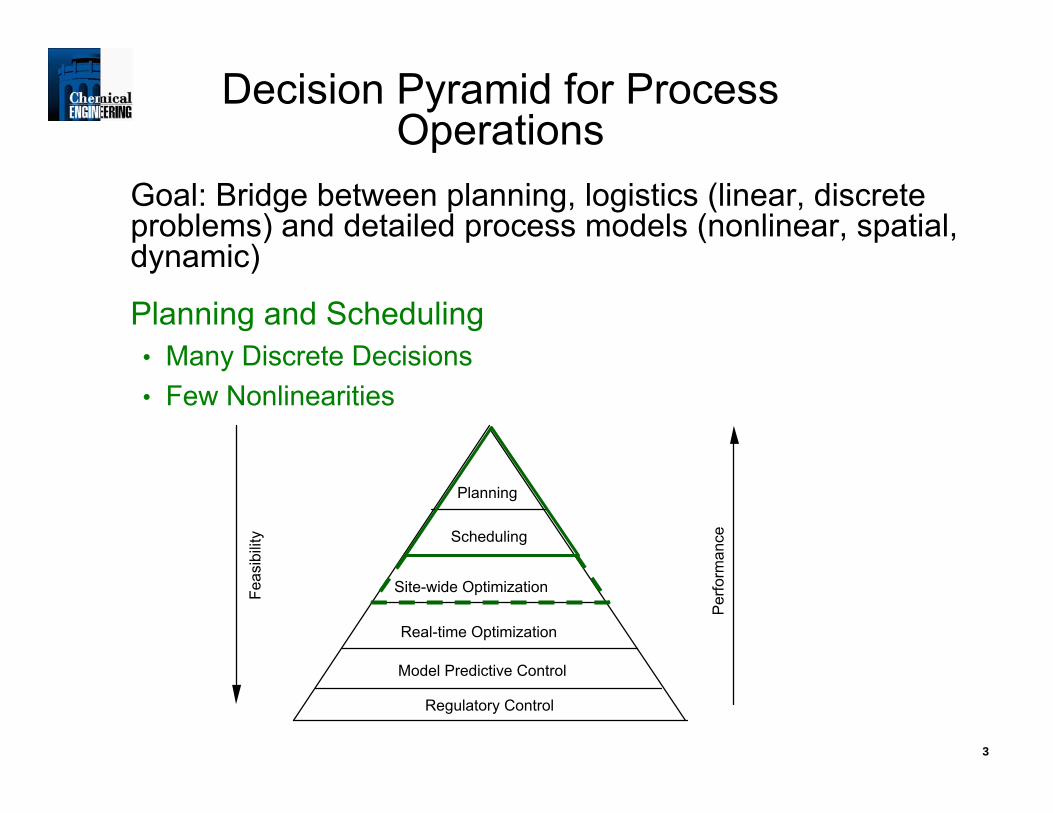
Goal: Bridge between planning, logistics (linear, discrete problems) and detailed process models (nonlinear, spatial, dynamic)

Planning and Scheduling• Many Discrete Decisions• Few Nonlinearities

Planning

Scheduling

Site-wide Optimization

Real-time Optimization

Model Predictive Control

Regulatory Control

Feas

ibili

ty

Per

form

ance

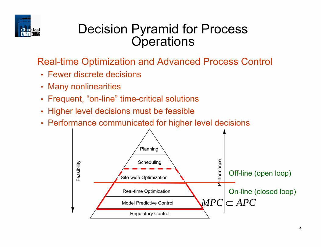
Decision Pyramid for Process Operations

4

Real-time Optimization and Advanced Process Control• Fewer discrete decisions• Many nonlinearities• Frequent, “on-line” time-critical solutions• Higher level decisions must be feasible• Performance communicated for higher level decisions

Planning

Scheduling

Site-wide Optimization

Real-time Optimization

Model Predictive Control

Regulatory Control

Feas

ibili

ty

Per

form

ance

Decision Pyramid for Process Operations

APCMPC ⊂

Off-line (open loop)

On-line (closed loop)

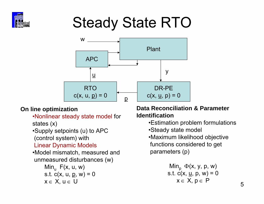
Steady State RTO

Data Reconciliation & Parameter Identification

•Estimation problem formulations•Steady state model•Maximum likelihood objective functions considered to get parameters (p)

Minp Φ(x, y, p, w)s.t. c(x, u, p, w) = 0

x ∈ X, p ∈ P

Plant

DR-PEc(x, u, p) = 0

RTOc(x, u, p) = 0

APC

y

p

u

w

On line optimization•Nonlinear steady state model for states (x)•Supply setpoints (u) to APC (control system) withLinear Dynamic Models•Model mismatch, measured and unmeasured disturbances (w)

Minu F(x, u, w)s.t. c(x, u, p, w) = 0x ∈ X, u ∈ U 5

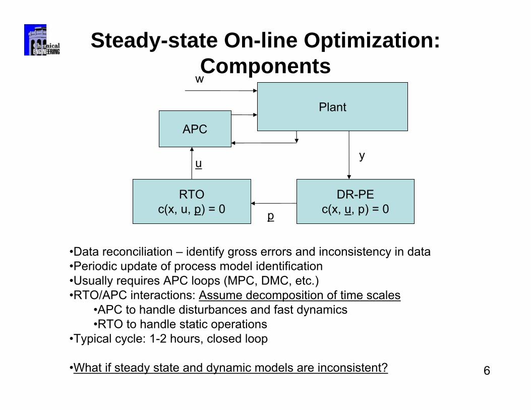
Steady-state On-line Optimization: Components

Plant

DR-PEc(x, u, p) = 0

RTOc(x, u, p) = 0

APC

y

p

u

w

•Data reconciliation – identify gross errors and inconsistency in data•Periodic update of process model identification •Usually requires APC loops (MPC, DMC, etc.)•RTO/APC interactions: Assume decomposition of time scales

•APC to handle disturbances and fast dynamics•RTO to handle static operations

•Typical cycle: 1-2 hours, closed loop

•What if steady state and dynamic models are inconsistent? 6

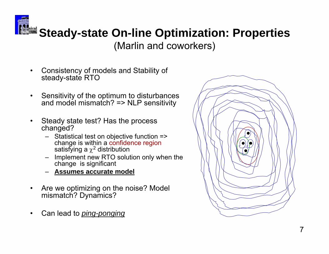
Steady-state On-line Optimization: Properties(Marlin and coworkers)

• Consistency of models and Stability of steady-state RTO

• Sensitivity of the optimum to disturbances and model mismatch? => NLP sensitivity

• Steady state test? Has the process changed?

– Statistical test on objective function => change is within a confidence regionsatisfying a χ2 distribution

– Implement new RTO solution only when the change is significant

– Assumes accurate model

• Are we optimizing on the noise? Model mismatch? Dynamics?

• Can lead to ping-ponging

7

Why Dynamic RTO?

• Batch processes• Grade transitions• Cyclic reactors (coking, regeneration…)• Cyclic processes (PSA, SMB…)• Continuous processes are never in steady state:

– Feed changes– Nonstandard operations– Optimal disturbance rejections

• Simulation environments (e.g., ACM, gPROMS) and first principle dynamic models are widely used for off-line studies

8

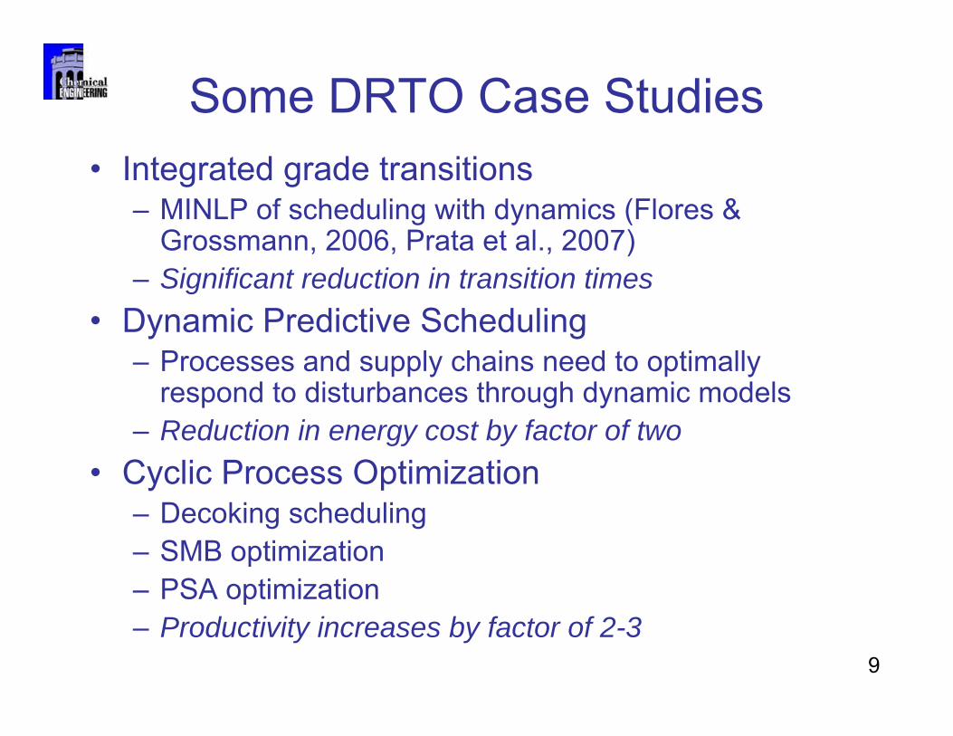
Some DRTO Case Studies• Integrated grade transitions

– MINLP of scheduling with dynamics (Flores & Grossmann, 2006, Prata et al., 2007)

– Significant reduction in transition times • Dynamic Predictive Scheduling

– Processes and supply chains need to optimally respond to disturbances through dynamic models

– Reduction in energy cost by factor of two• Cyclic Process Optimization

– Decoking scheduling– SMB optimization– PSA optimization– Productivity increases by factor of 2-3

9

10

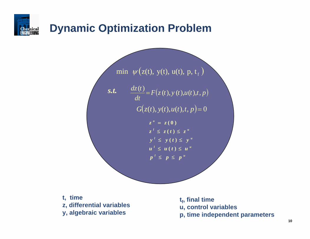
tf, final timeu, control variablesp, time independent parameters

t, timez, differential variablesy, algebraic variables

Dynamic Optimization Problem

( )ftp,u(t),y(t),z(t), ψmin

( )pttutytzFdt

tdz ,),(),(),()(=

( ) 0,),(),(),( =pttutytzG

ul

ul

ul

ul

o

ppputuuytyy

ztzzzz

≤≤

≤≤

≤≤

≤≤

=

)()(

)()0(

s.t.

11

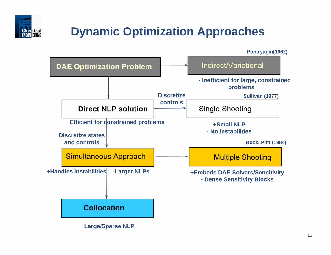
Dynamic Optimization Approaches

DAE Optimization Problem

Multiple Shooting

+Embeds DAE Solvers/Sensitivity- Dense Sensitivity Blocks

+Handles instabilities

Single Shooting

Sullivan (1977)

+Small NLP - No instabilities

Discretize controls

Collocation

Large/Sparse NLP

Direct NLP solutionEfficient for constrained problems

Simultaneous Approach

-Larger NLPs

Discretize states and controls

Indirect/Variational

Pontryagin(1962)

- Inefficient for large, constrained problems

Bock, Plitt (1984)

12

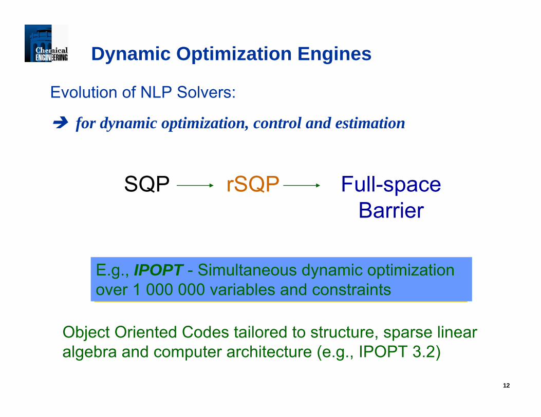
Dynamic Optimization Engines

Evolution of NLP Solvers:

for dynamic optimization, control and estimation

E.g., NPSOL and Sequential Dynamic Optimization - over 100 variables and constraints E.g, SNOPT and Multiple Shooting - over 100 d.f.s but over 105 variables and constraintsE.g., IPOPT - Simultaneous dynamic optimizationover 1 000 000 variables and constraints

SQP rSQP Full-spaceBarrier

Object Oriented Codes tailored to structure, sparse linearalgebra and computer architecture (e.g., IPOPT 3.2)

13

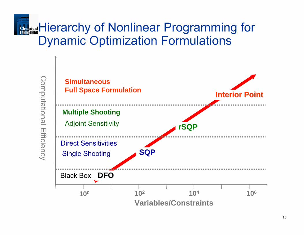
Hierarchy of Nonlinear Programming for Dynamic Optimization Formulations

Variables/Constraints102 104 106

Black Box

Direct SensitivitiesSingle Shooting

Multiple ShootingAdjoint Sensitivity

Simultaneous Full Space Formulation

100

SQPSQP

rSQPrSQP

Interior PointInterior Point

DFODFO

Com

putational Efficiency

14

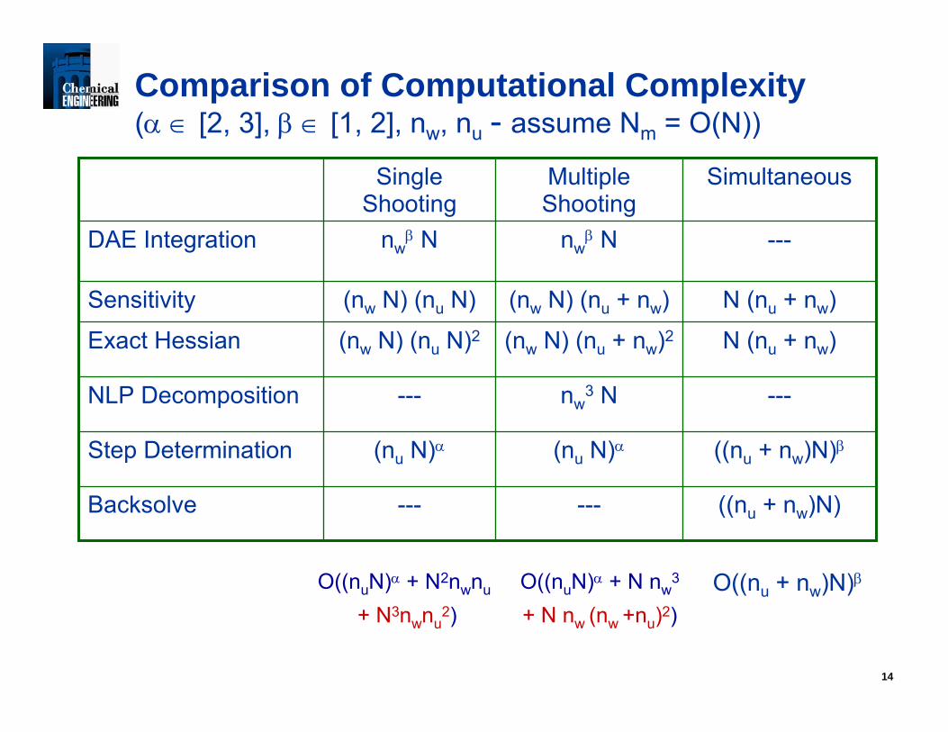
Comparison of Computational Complexity(α ∈ [2, 3], β ∈ [1, 2], nw, nu - assume Nm = O(N))

((nu + nw)N)------Backsolve

((nu + nw)N)β(nu N)α(nu N)αStep Determination

---nw3 N---NLP Decomposition

N (nu + nw)(nw N) (nu + nw)2(nw N) (nu N)2Exact Hessian

N (nu + nw)(nw N) (nu + nw)(nw N) (nu N)Sensitivity

---nwβ Nnw

β NDAE Integration

SimultaneousMultiple Shooting

Single Shooting

O((nuN)α + N2nwnu

+ N3nwnu2)

O((nuN)α + N nw3

+ N nw (nw +nu)2)O((nu + nw)N)β

15

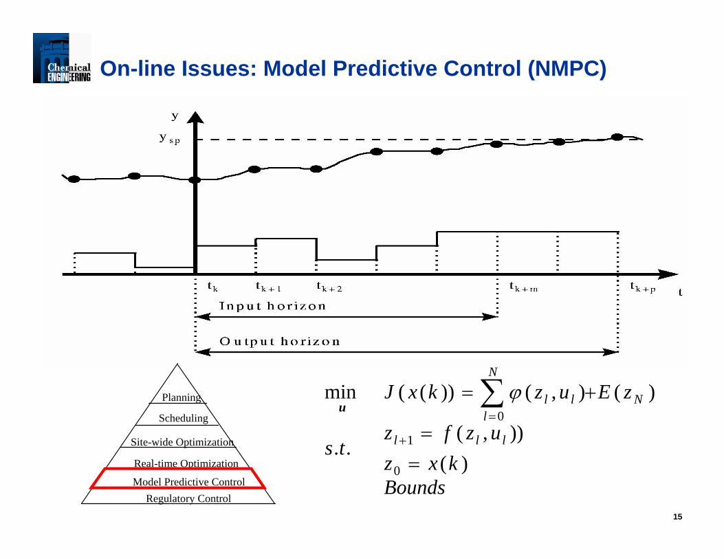
On-line Issues: Model Predictive Control (NMPC)

Process

NMPC Controller

d : disturbancesz : differential statesy : algebraic states

u : manipulatedvariables

ysp : set points

( )( )dpuyzG

dpuyzFz,,,,0,,,,

==′

NMPC Estimation and Control

Boundskxz

uzfzts

zEuzkxJ

lll

N

lNll

)()),(

..

)(),())((min

0

1

0

==

+=

+

=∑ϕ

u

NMPC Subproblem

Why NMPC?ν Track a profile – evolve from

linear dynamic models (MPC)ν Severe nonlinear dynamics (e.g,

sign changes in gains)ν Operate process over wide range

(e.g., startup and shutdown)

Model Updater( )( )dpuyzG

dpuyzFz,,,,0,,,,

==′

Planning

Scheduling

Site-wide Optimization

Real-time Optimization

Model Predictive ControlRegulatory Control

16

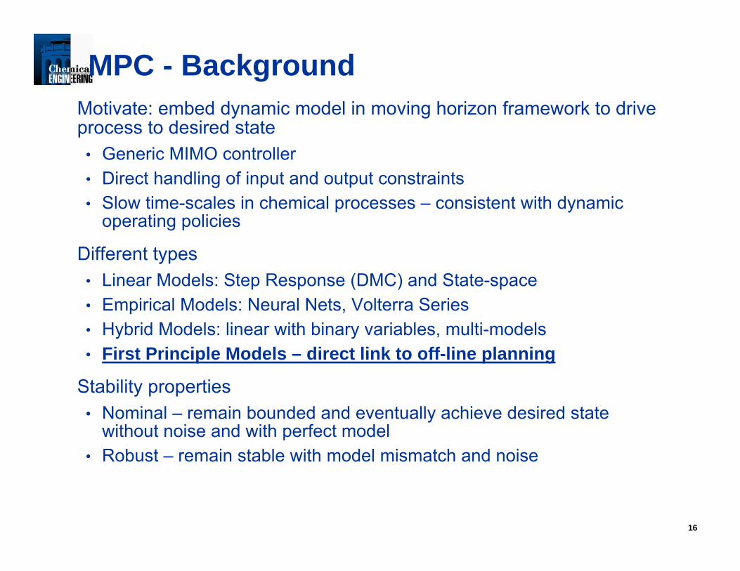
MPC - BackgroundMotivate: embed dynamic model in moving horizon framework to drive process to desired state

• Generic MIMO controller • Direct handling of input and output constraints• Slow time-scales in chemical processes – consistent with dynamic

operating policies

Different types• Linear Models: Step Response (DMC) and State-space• Empirical Models: Neural Nets, Volterra Series• Hybrid Models: linear with binary variables, multi-models• First Principle Models – direct link to off-line planning

Stability properties• Nominal – remain bounded and eventually achieve desired state

without noise and with perfect model• Robust – remain stable with model mismatch and noise

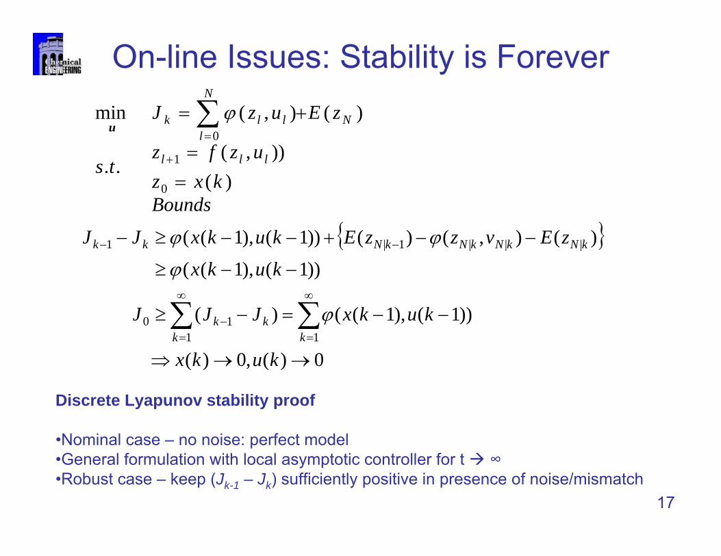
On-line Issues: Stability is Forever

Discrete Lyapunov stability proof

•Nominal case – no noise: perfect model•General formulation with local asymptotic controller for t ∞•Robust case – keep (Jk-1 – Jk) sufficiently positive in presence of noise/mismatch

{ }

0)(,0)(

))1(),1(()(

))1(),1((

)(),()())1(),1((

1110

|||1|1

→→⇒

−−=−≥

−−≥

−−+−−≥−

∑∑∞

=

∞

=−

−−

kukx

kukxJJJ

kukx

zEvzzEkukxJJ

kkkk

kNkNkNkNkk

ϕ

ϕ

ϕϕ

17

Boundskxz

uzfzts

zEuzJ

lll

N

lNllk

)()),(

..

)(),(min

0

1

0

==

+=

+

=∑ϕ

u

18

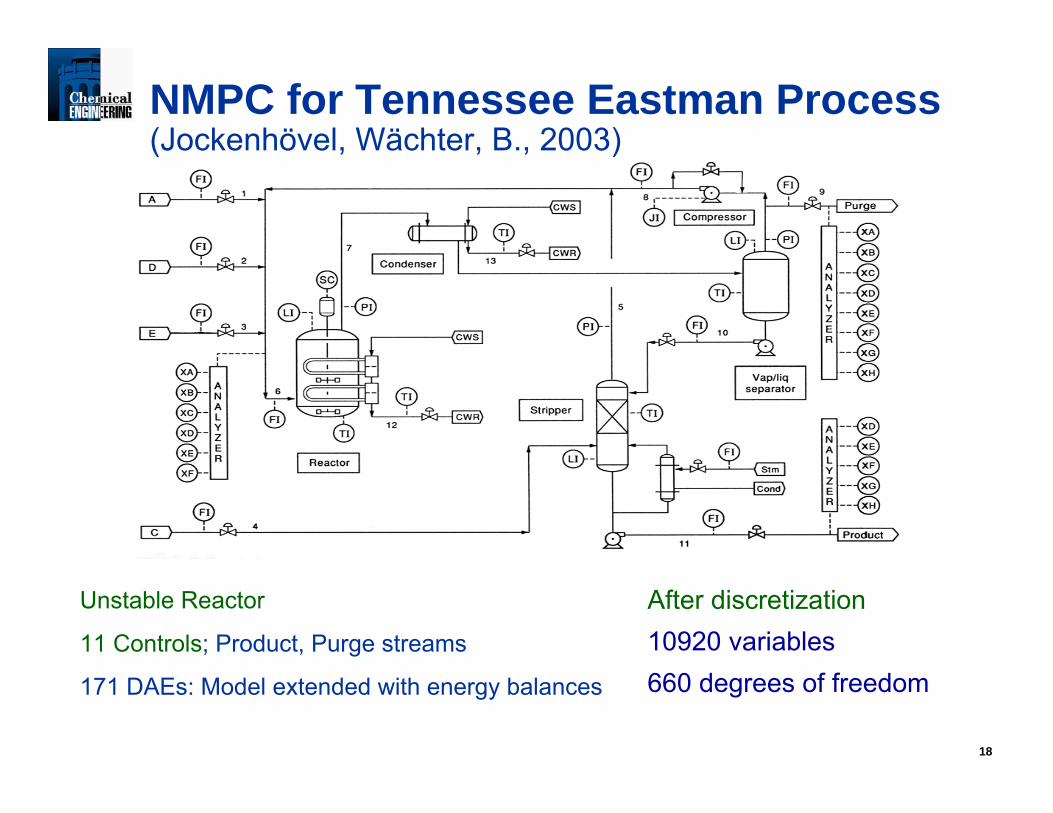
NMPC for Tennessee Eastman Process(Jockenhövel, Wächter, B., 2003)

Unstable Reactor

11 Controls; Product, Purge streams

171 DAEs: Model extended with energy balances

After discretization10920 variables660 degrees of freedom

19

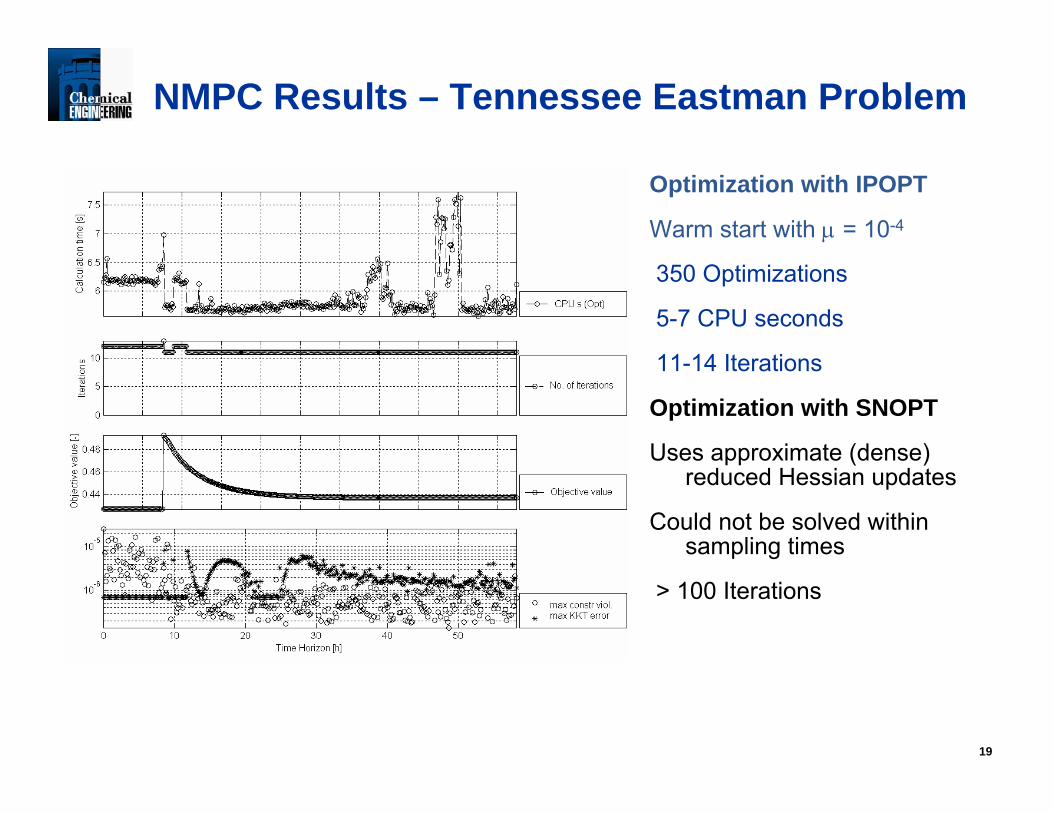
NMPC Results – Tennessee Eastman Problem

Optimization with IPOPT

Warm start with μ = 10-4

350 Optimizations

5-7 CPU seconds

11-14 Iterations

Optimization with SNOPT

Uses approximate (dense) reduced Hessian updates

Could not be solved within sampling times

> 100 Iterations

20

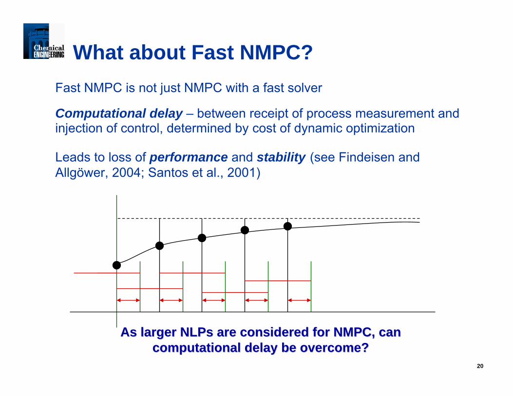
What about Fast NMPC?Fast NMPC is not just NMPC with a fast solver

Computational delay – between receipt of process measurement and injection of control, determined by cost of dynamic optimization

Leads to loss of performance and stability (see Findeisen and Allgöwer, 2004; Santos et al., 2001)

As larger As larger NLPsNLPs are considered for NMPC, can are considered for NMPC, can computational delay be overcome?computational delay be overcome?

21

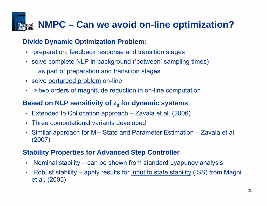
NMPC – Can we avoid on-line optimization?Divide Dynamic Optimization Problem:

• preparation, feedback response and transition stages • solve complete NLP in background (‘between’ sampling times)

as part of preparation and transition stages• solve perturbed problem on-line• > two orders of magnitude reduction in on-line computation

Based on NLP sensitivity of z0 for dynamic systems• Extended to Collocation approach – Zavala et al. (2006)• Three computational variants developed• Similar approach for MH State and Parameter Estimation – Zavala et al.

(2007)

Stability Properties for Advanced Step Controller• Nominal stability – can be shown from standard Lyapunov analysis• Robust stability – apply results for input to state stability (ISS) from Magni

et al. (2005)

22

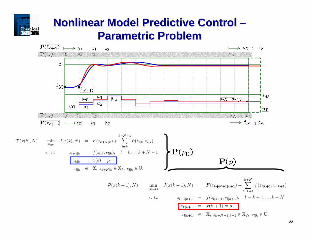
Nonlinear Model Predictive Control Nonlinear Model Predictive Control ––Parametric ProblemParametric Problem

23

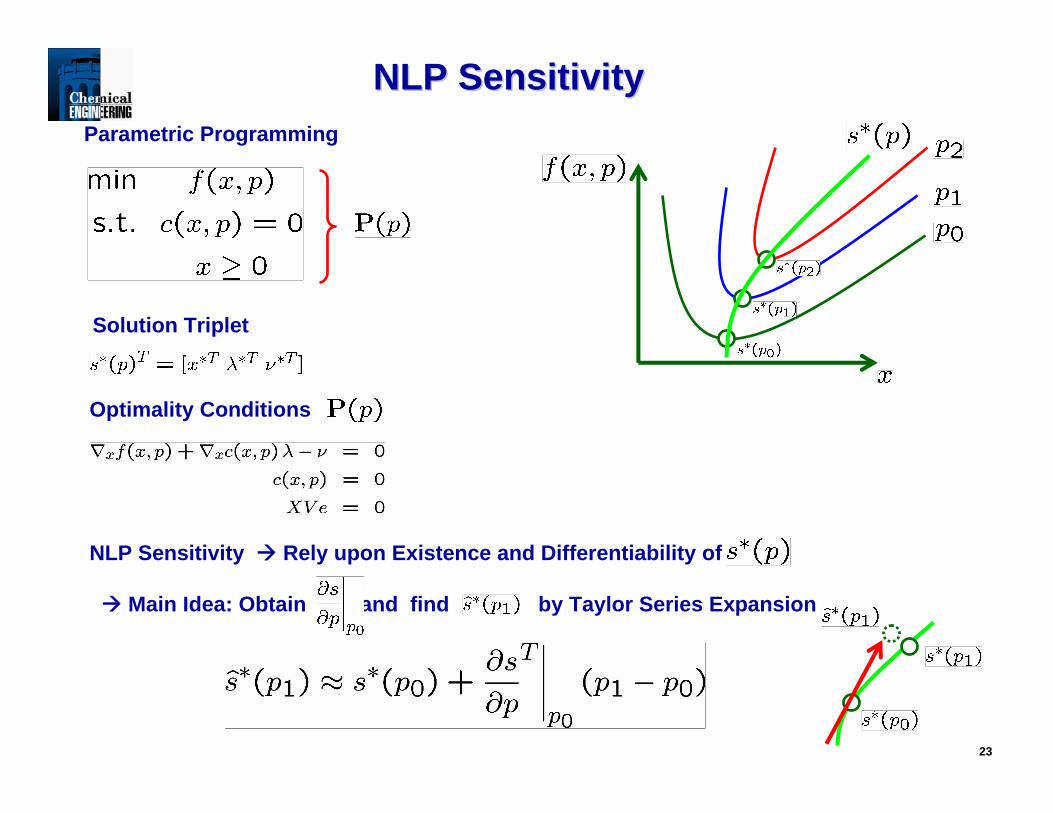
NLP SensitivityNLP SensitivityParametric Programming

NLP Sensitivity Rely upon Existence and Differentiability of Path

Main Idea: Obtain and find by Taylor Series Expansion

Optimality Conditions

Solution Triplet

24

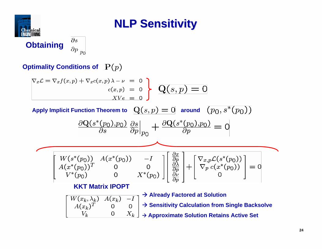
NLP SensitivityNLP Sensitivity

Optimality Conditions of

Obtaining

Already Factored at Solution

Sensitivity Calculation from Single Backsolve

Approximate Solution Retains Active Set

KKT Matrix IPOPT

Apply Implicit Function Theorem to around

25

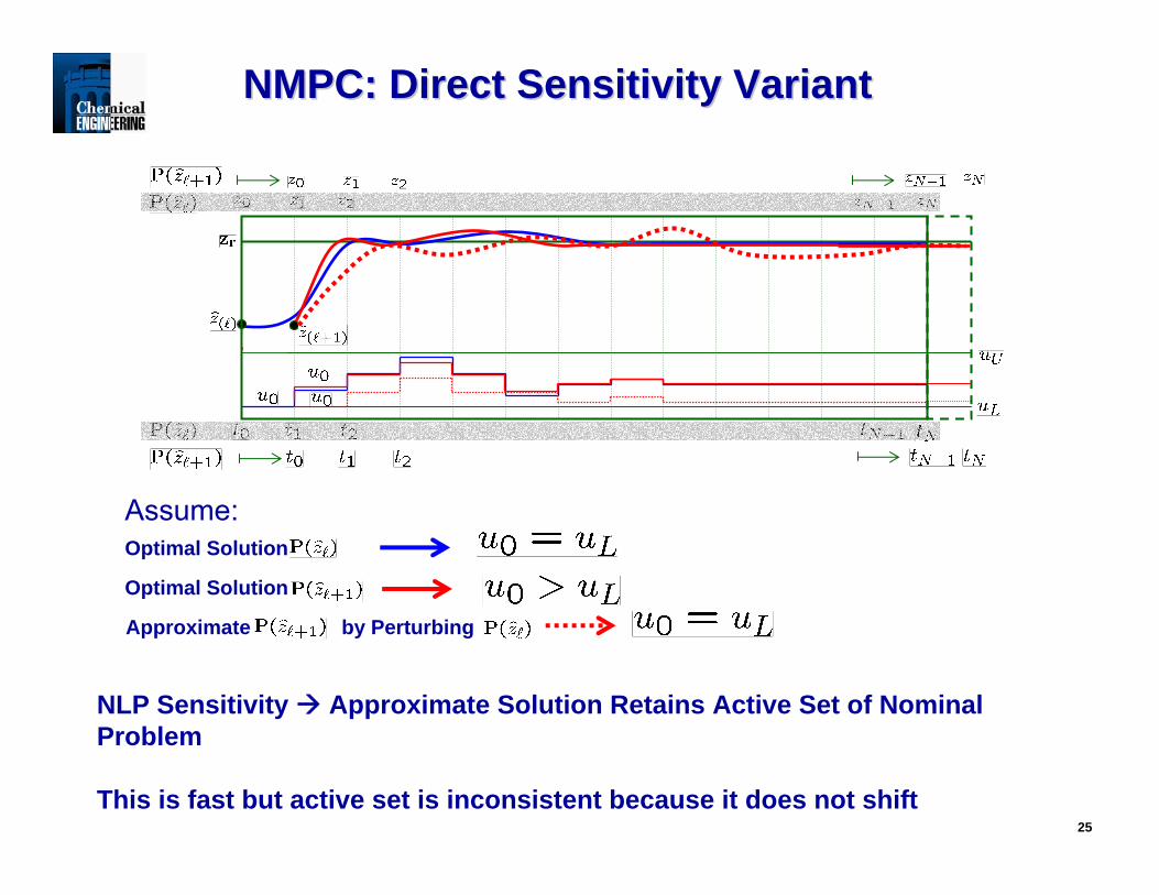
NMPC: Direct Sensitivity VariantNMPC: Direct Sensitivity Variant

Optimal Solution

Optimal Solution

Approximate by Perturbing

NLP Sensitivity Approximate Solution Retains Active Set of Nominal Problem

This is fast but active set is inconsistent because it does not shift

Assume:

26

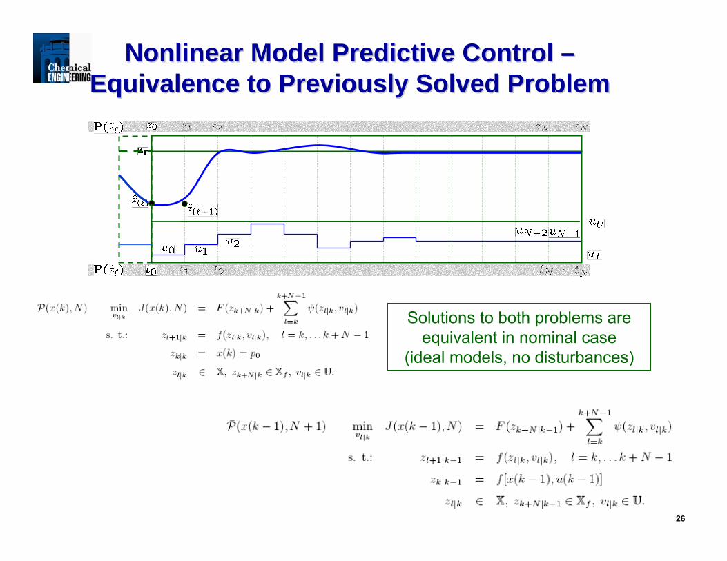
Nonlinear Model Predictive Control Nonlinear Model Predictive Control ––Equivalence to Previously Solved ProblemEquivalence to Previously Solved Problem

Solutions to both problems are equivalent in nominal case

(ideal models, no disturbances)

27

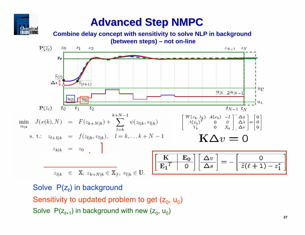
Advanced Step NMPCAdvanced Step NMPCCombine delay concept with sensitivity to solve NLP in background

(between steps) – not on-line

Solve P(zℓ) in backgroundSensitivity to updated problem to get (z0, u0)Solve P(zℓ+1) in background with new (z0, u0)

28

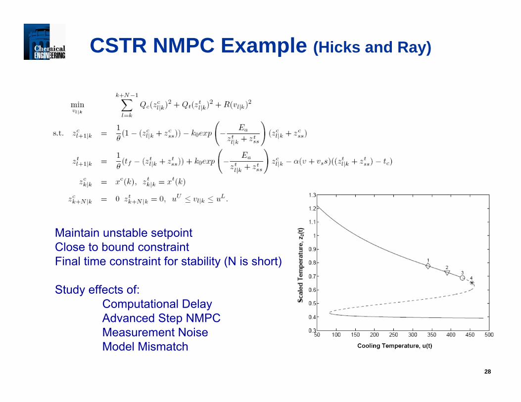
CSTR NMPC Example (Hicks and Ray)

Maintain unstable setpointClose to bound constraintFinal time constraint for stability (N is short)

Study effects of:Computational DelayAdvanced Step NMPCMeasurement NoiseModel Mismatch

29

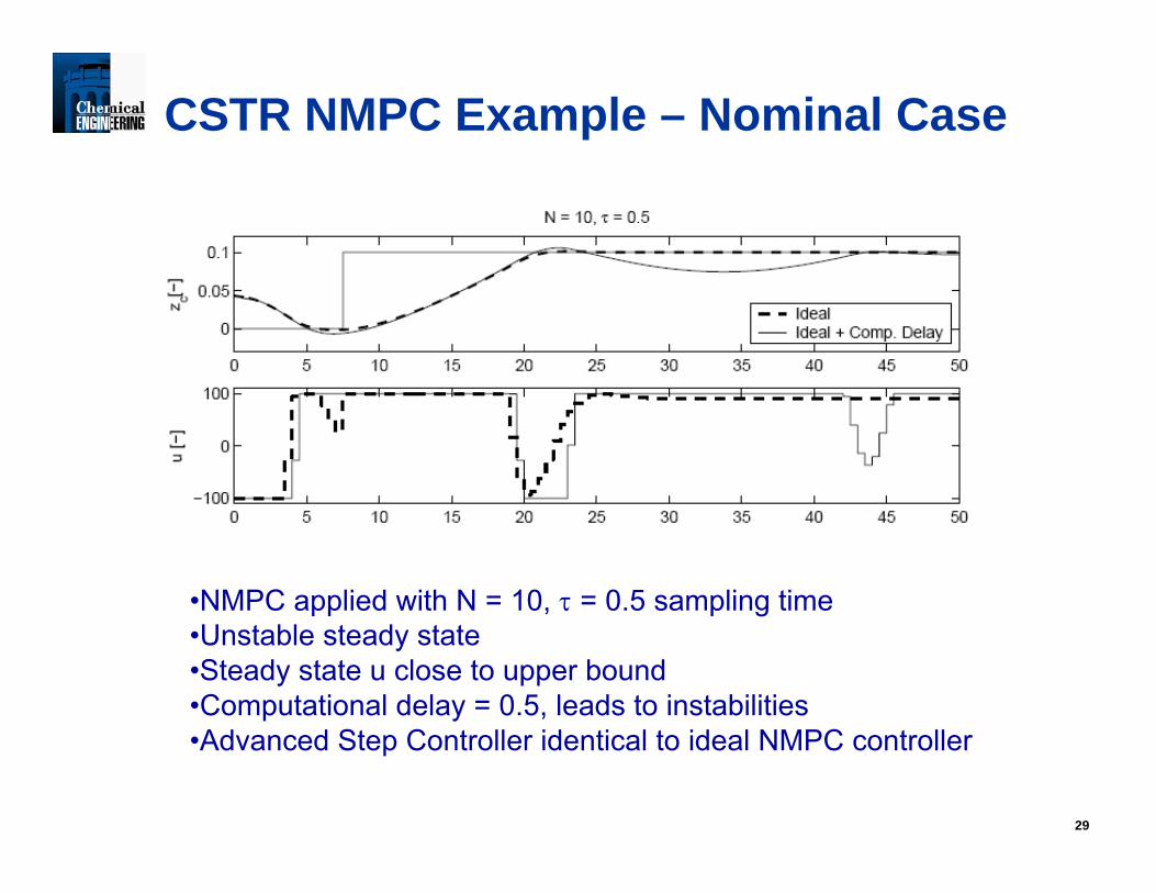
CSTR NMPC Example – Nominal Case

•NMPC applied with N = 10, τ = 0.5 sampling time•Unstable steady state•Steady state u close to upper bound•Computational delay = 0.5, leads to instabilities•Advanced Step Controller identical to ideal NMPC controller

30

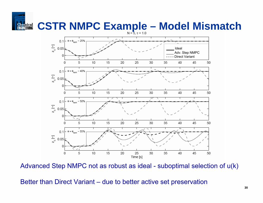
CSTR NMPC Example – Model Mismatch

Advanced Step NMPC not as robust as ideal - suboptimal selection of u(k)

Better than Direct Variant – due to better active set preservation

___ Ideal____ Adv. Step NMPC- - - - Direct Variant

31

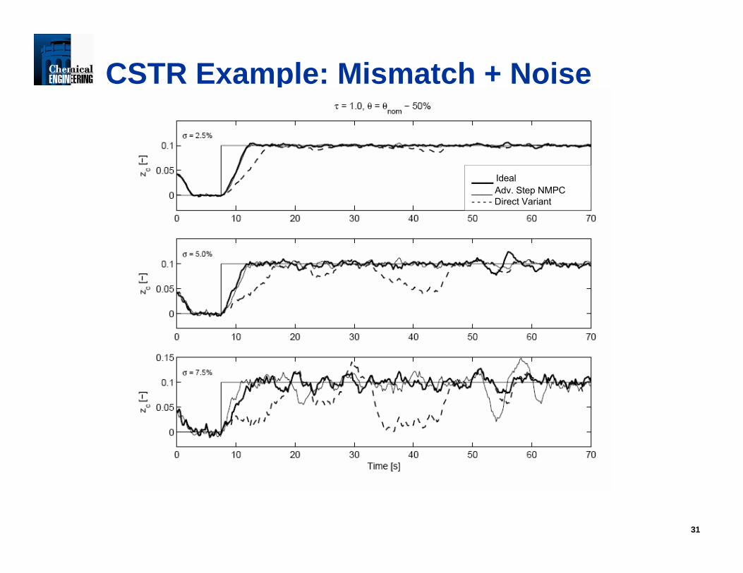
CSTR Example: Mismatch + Noise

___ Ideal____ Adv. Step NMPC- - - - Direct Variant

32

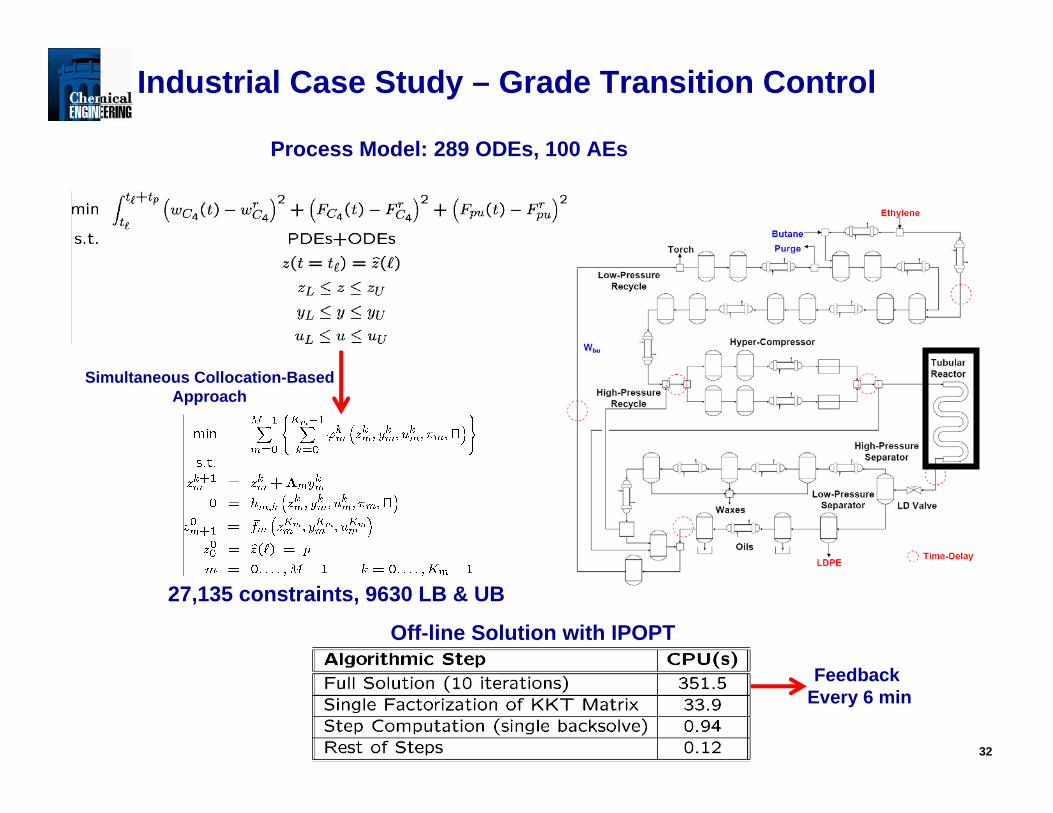
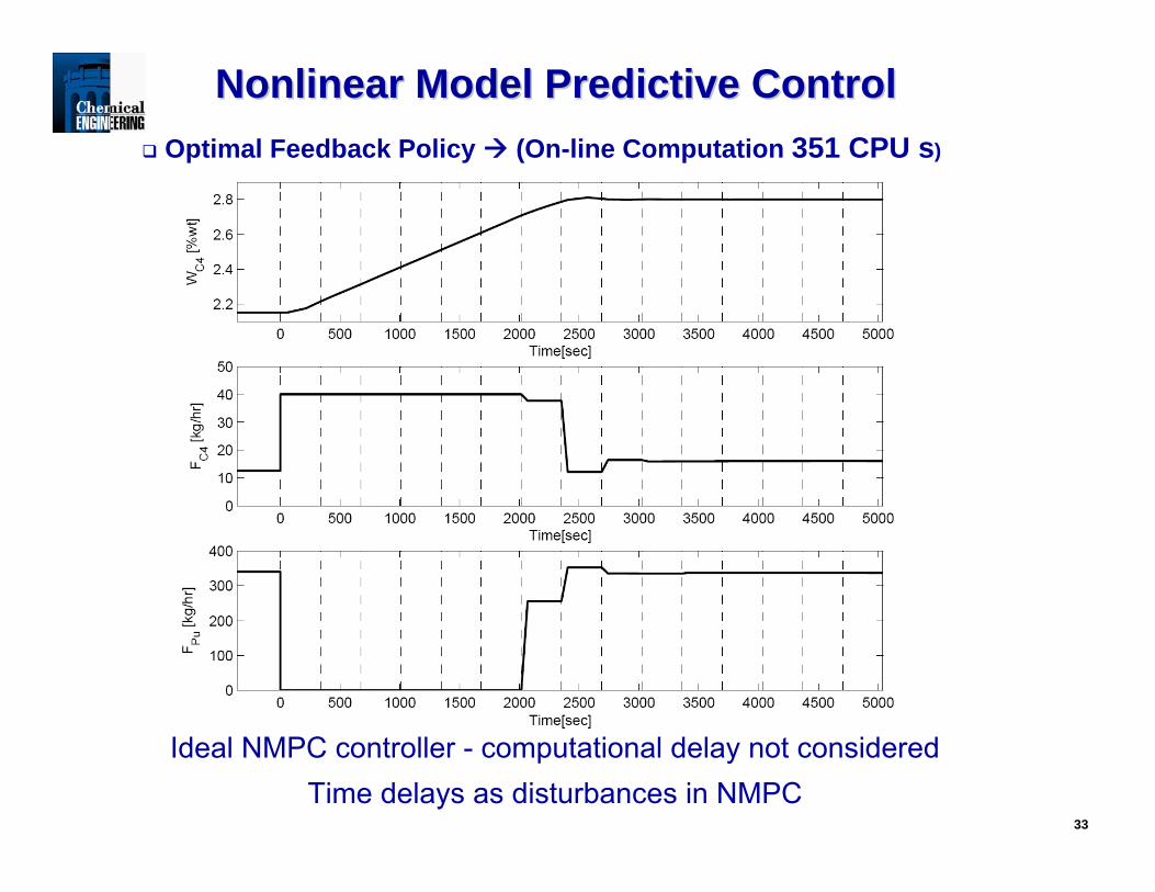
Industrial Case Study – Grade Transition Control

Simultaneous Collocation-BasedApproach

27,135 constraints, 9630 LB & UB

Off-line Solution with IPOPT

Feedback Every 6 min

Process Model: 289 ODEs, 100 AEs

33

Nonlinear Model Predictive ControlNonlinear Model Predictive ControlOptimal Feedback Policy (On-line Computation 351 CPU s)

Ideal NMPC controller - computational delay not consideredTime delays as disturbances in NMPC

34

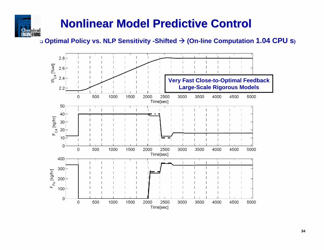
Nonlinear Model Predictive ControlNonlinear Model Predictive ControlOptimal Policy vs. NLP Sensitivity -Shifted (On-line Computation 1.04 CPU s)

Very Fast Close-to-Optimal FeedbackLarge-Scale Rigorous Models

35

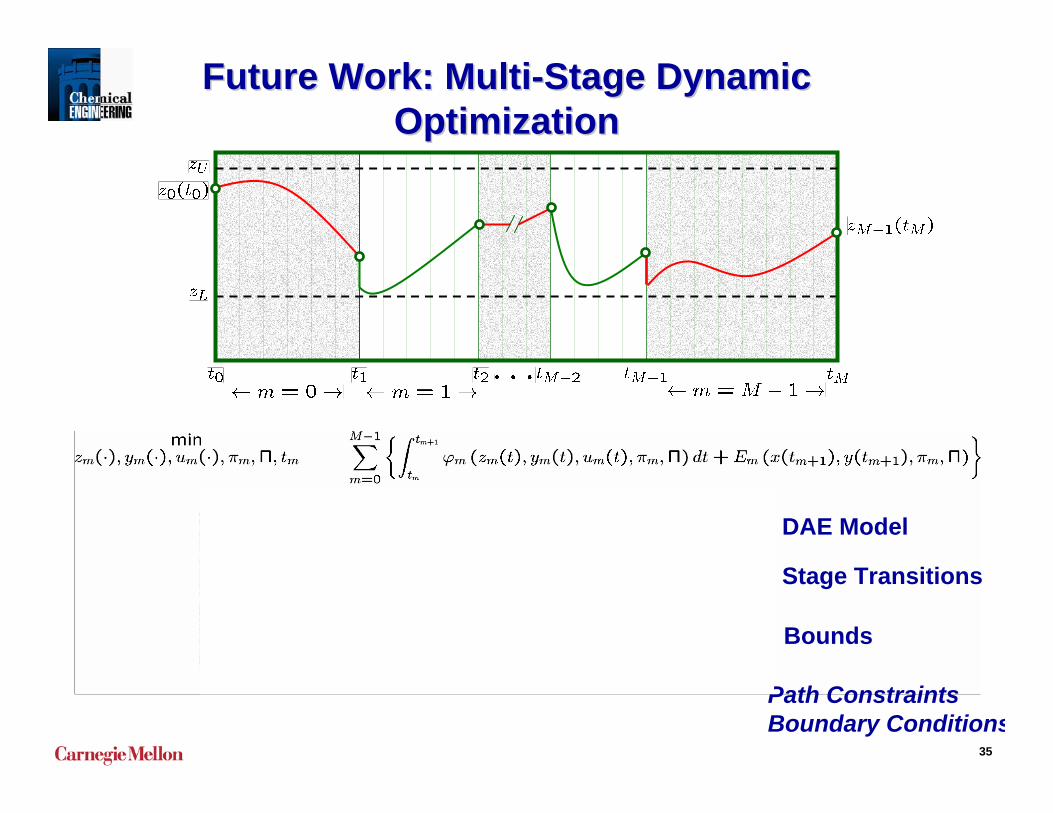
Future Work: MultiFuture Work: Multi--Stage Dynamic Stage Dynamic OptimizationOptimization

DAE Model

Stage Transitions

Bounds

Path ConstraintsBoundary Conditions

36

Multi-stage OptimizationDetermine Off-line policy• Tracking problem for NMPC• Nominal policy or incorporate uncertainty in conservative

way (no recourse due to policy tracking)

Determine On-line policy• Solve consistent economic objective through on-line

DRTO (NMPC that incorporates multi-stage with long horizons)

• Exploit uncertainty through recourse on trajectory optimization

– Retain stability and robustness– Incorporate feedforward measurements

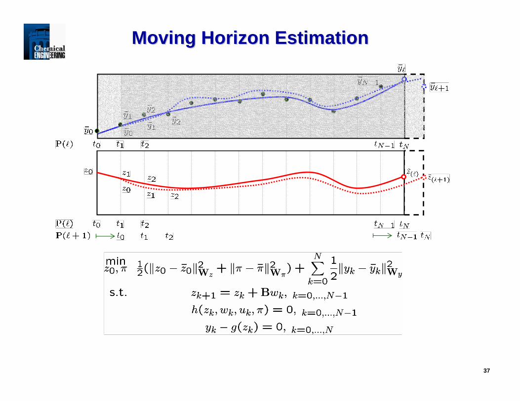
• Requires state and parameter estimation from plant– Use nonlinear model– Adopt Moving Horizon Estimation Formulation

37

Moving Horizon EstimationMoving Horizon Estimation

Process

NMPC Controller

d : disturbancesz : differential statesy : algebraic states

u : manipulatedvariables

ysp : set points

( )( )dpuyzG

dpuyzFz,,,,0,,,,

==′

Model Updater( )( )dpuyzG

dpuyzFz,,,,0,,,,

==′

38

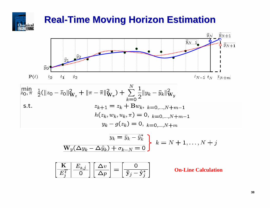
RealReal--Time Moving Horizon EstimationTime Moving Horizon Estimation

On-Line Calculation

39

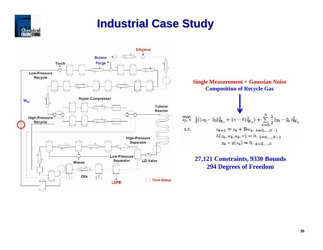
Industrial Case StudyIndustrial Case Study

Single Measurement + Gaussian NoiseComposition of Recycle Gas

27,121 Constraints, 9330 Bounds294 Degrees of Freedom

40

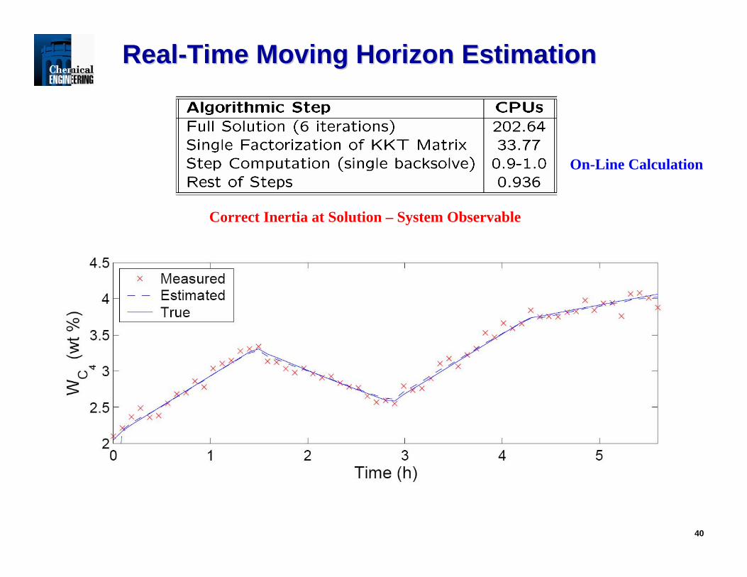
RealReal--Time Moving Horizon EstimationTime Moving Horizon Estimation

Correct Inertia at Solution – System Observable

On-Line Calculation

Summary• RTO and MPC widely used for refineries, ethylene and,

more recently, chemical plants – Inconsistency in models– Can lead to operating problems

• Off-line dynamic optimization is widely used – Polymer processes (especially grade transitions)– Batch processes– Periodic processes

• NMPC provides link for off-line and on-line optimization– Stability and robustness properties– Advanced step controller leads to very fast calculations

• Analogous stability and robustness properties• On-line cost is negligible

• Multi-stage planning and on-line switches– Leads to exploitation of uncertainty (on-line recourse) – Avoids conservative performance– Update model with MHE– Evolve from regulatory NMPC to Large-scale DRTO

41

ReferencesF. Allgöwer and A. Zheng (eds.), Nonlinear Model Predictive Control, Birkhaeuser, Basel (2000)

R. D. Bartusiak, “NLMPC: A platform for optimal control of feed- or product-flexible manufacturing,” in Nonlinear Model Predictive Control 05, Allgower, Findeisen, Biegler (eds.), Springer, to appear

Biegler Homepage: http://dynopt.cheme.cmu.edu/papers.htm

Forbes, J. F. and Marlin, T. E.. Model Accuracy for Economic Optimizing Controllers: The Bias Update Case. Ind.Eng.Chem.Res. 33, 1919-1929. 1994

Forbes, J. F. and Marlin, T. E.. “Design Cost: A Systematic Approach to Technology Selection for Model-Based Real-Time Optimization Systems,” Computers Chem.Engng. 20[6/7], 717-734. 1996

Grossmann Homepage: http://egon.cheme.cmu.edu/papers.html

M. Grötschel, S. Krumke, J. Rambau (eds.), Online Optimization of Large Systems, Springer, Berlin (2001)

K. Naidoo, J. Guiver, P. Turner, M. Keenan, M. Harmse “Experiences with Nonlinear MPC in Polymer Manufacturing,” in Nonlinear Model Predictive Control 05, Allgower, Findeisen, Biegler (eds.), Springer, to appear

Yip, W. S. and Marlin, T. E. “Multiple Data Sets for Model Updating in Real-Time Operations Optimization,” Computers Chem.Engng. 26[10], 1345-1362. 2002.

42

References – Some DRTO Case Studies

Busch, J.; Oldenburg, J.; Santos, M.; Cruse, A.; Marquardt, W. Dynamicpredictive scheduling of operational strategies for continuous processes using mixed-logic dynamic optimization, Comput. Chem. Eng., 2007, 31, 574-587.

Flores-Tlacuahuac, A.; Grossmann, I.E. Simultaneous cyclic scheduling andcontrol of a multiproduct CSTR, Ind. Eng. Chem. Res., 2006, 27, 6698-6712.

Kadam, J.; Srinivasan, B., Bonvin, D., Marquardt, W. Optimal grade transition in industrial polymerization processes via NCO tracking. AIChE J., 2007, 53, 3, 627-639.

Oldenburg, J.; Marquardt, W.; Heinz D.; Leineweber, D. B., Mixed-logic dynamic optimization applied to batch distillation process design, AIChE J. 2003, 48(11), 2900- 2917.

E Perea, B E Ydstie and I E Grossmann, A model predictive control strategy for supply chain optimization, Comput. Chem. Eng., 2003, 27, 1201-1218.

M. Liepelt, K Schittkowski, Optimal control of distributed systems with breakpoints, p. 271 in M. Grötschel, S. Krumke, J. Rambau (eds.), Online Optimization of Large Systems, Springer, Berlin (2001)

See also Biegler homepage

43