Embed Size (px)
Citation preview

Coordinating Inventory Control and Pricing
Strategies for Perishable Products
Xin Chen
International Center of Management Science and Engineering
Nanjing University, Nanjing 210093, China, and
Department of Industrial and Enterprise Systems Engineering
University of Illinois at Urbana-Champaign, Urbana, IL 61801, [email protected]
Zhan Pang
International Center of Management Science and Engineering
Nanjing University, Nanjing 210093, China, and
Lancaster University Management School
Lancaster LA1 4YX, United Kingdom, [email protected]
Limeng Pan
Department of Industrial and Enterprise Systems Engineering
University of Illinois at Urbana-Champaign, Urbana, IL 61801, [email protected]
Abstract: We analyze a joint pricing and inventory control problem for a perishable product with a fixed
lifetime over a finite horizon. In each period, demand depends on the price of the current period plus an
additive random term. Inventories can be intentionally disposed of and those that reach their lifetime have
to be disposed of. The objective is to find a joint pricing, ordering, and disposal policy so as to maximize the
total expected discounted profit over the planning horizon taking into account linear ordering cost, inventory
holding and backlogging or lost-sales penalty cost and disposal cost. Employing the concept of L\-concavity,
we show some monotonicity properties of the optimal policies. Our results shed new light on perishable
inventory management, and our approach provides a significantly simpler proof of a classical structural result
in the literature. Moreover, we identify bounds on the optimal order-up-to levels and develop an effective
heuristic policy. Numerical results show that our heuristic policy performs well in both stationary and non-
stationary settings. Finally, we show that our approach also applies to models with random lifetimes and
inventory rationing models with multiple demand classes.
Key words : Perishable inventory management, pricing strategies, L\-convexity
History : September 2012, July 2013, November 2013, January 2014
1. Introduction
The U.S. grocery industry is a very competitive market where more than two-thirds of industrial
stores are supermarkets. The majority of sales revenue of grocery stores and supermarkets comes
from perishables such as food items (e.g., meats and poultry, produce, dairy, and bakery products),
pharmaceuticals (e.g., drugs and vitamins), and cut flowers. For instance, Food Market Institute
1

2 Chen, Pang and Pan: Coordinating Inventory Control and Pricing Strategies for Perishable Products
(2006) reports that perishables accounted for 50.12% of the total 2005 supermarket sales revenue
of about $383 billion. The number was even higher in 2010 at 50.62% of $444 billion total sales
revenue.
In grocery retailing, spoilage from perishables represents a major threat to the profitability of
supermarkets. As quoted in a white paper of Power-ID, a radio frequency identification (RFID)
technology company, “A survey by the National Supermarket Research Group found that a 300-
store grocery chain loses about $34 million a year due to spoilage. On an industry-wide level, losses
due to spoilage and shrinkage translate into $32 billion for chilled meats, seafood, and cheese; $34
billion for produce; and $5.4 billion for pharmaceutical and biomedical products (EPCGlobal).” 1
Thus, effective inventory management of perishables is crucial for the success in grocery retailing.
The 2012 National Supermarket Shrink Survey reveals that “there exists a clear thread of practices
associated with the control of inventory, inventory turnover and inventory management with result-
ing shrink loss levels. Top performing companies report having 26% lower inventory levels results
in 30% more inventory turns and 15% lower shrink than companies without clear and consistently
executed inventory control practices.”2
Pricing is another important and effective lever to manage the profitability of perishables in
retailing. Of course, it is a double-edged sword. A poor pricing strategy can also easily damage the
profitability of a firm. For example, Tesco, the largest grocery retailer in the UK, failed to revive
its sales despite spending £500 million on price cuts and as a result its CEO quit3. Compared to
those simple pricing strategies that may change prices dramatically, it could be more appropriate
to adjust the price in a dynamic fashion, which enables price changes according to the availability
of inventory and products’ residual shelf lives.
The advances of information technologies such as RFID tags allow retailers to accurately track
product flows and make pricing and inventory decisions dynamically to better align supply with
demand. The emergence of online grocery stores (e.g., AmazonFresh - a subsidiary of the Ama-
zon.com) further facilitates the adoption of dynamic pricing strategies. A recent industry study
sponsored by IBM (Webber et al. 2011) highlights that dynamic pricing can help retailers to effec-
tively reduce food wastage by enabling the retailer to be more reactive to things like unexpected
weather. This report also provides a case study which describes how a Dutch grocery retailer Albert
Heijn experimented the integrated dynamic pricing and inventory control policies in one of its
stores.
1 http://www.power-id.com/Data/pdf/PowerTMP White Paper.pdf, accessed on Jan 20, 2012.
2 http://www.retailcontrol.com/articles/time-to-get-your-stock-levels-in-line-and-overall-inventory-under-control/,
accessed on 13 August, 2012
3 http://www.bbc.co.uk/news/business-17378409, accessed on Aug 13, 2012

Chen, Pang and Pan: Coordinating Inventory Control and Pricing Strategies for Perishable Products 3
Similar issues are also faced by blood banks and pharmacies (Karaesmen et al. 2011, Pierskalla
2004). According to the 2009 national blood collection and utilization survey report, 4.7% of all
components of blood processed for transfusion were outdated in 2008 in the United States. In
particular, the outdated whole-blood-derived (WBD) platelets accounted for 24.4% of all WBD
platelets processed in 2008 (AABB 2009). Karaesmen et al. (2011) point out that there is pressing
need for research in the coordination of pricing and inventory management in blood supply chains,
which further confirms the relevance of our work.
A key feature of perishable inventory systems is that a product has a finite shelf-life and hence
the inventories of different ages for the same product may co-exist on the same shelf. Different from
the durable inventory systems, the joint inventory and pricing strategies for a perishable product
need to take into account the levels of the inventories of different ages and how inventories are
issued.
The majority of the perishable inventory literature assumes first-in-first-out (FIFO) issuing policy
(Nahmias 2011). This assumption is reasonable for blood inventory systems in which the blood
banks have the luxury of determining inventory issuing policy. It also applies to some grocery
retailers who only display the oldest items on the shelves to force customers to purchase oldest
inventories first. Under the FIFO issuing policy, retailers often post a single price for all the units
of a product at any point in time and may vary the price over time. It is natural for online grocery
stores such as AmazonFresh to adopt this pricing strategy and inventory issuing policy. Intuitively,
given the same total inventory level, the more aged inventory, the more likely the seller will set
a lower price to turn the inventory over more quickly and reduce outdating (Nahmias 1982). Our
model also assumes that the retailer can decide how to issue inventories and always post a single
price at any point in time.
Nevertheless, some retailers would allow customers to choose items of different ages on the same
shelves. In such a circumstance, if all the items are charged the same price, one can expect that
customers will choose the freshest items, resulting last in first out (LIFO) sequence. In practice,
retailers such as Bruegger’s Bagels offer discounts for aged items while keeping regular prices for
fresh ones. Some other retailers such as Chesapeake Bagel choose to dispose of old inventory as
new inventory is available for sales. See Ferguson and Koenigsberg (2007) and Li et al. (2012) for
more empirical evidences and discussions on different pricing and inventory control strategies.
In this paper, we analyze a joint inventory and pricing control problem for a retailer to manage
a perishable product in a periodic-review inventory system. At the beginning of each period, the
retailer decides how much to order and sets a single price for inventories of different ages. We
assume that the retailer can decide how to issue inventories. At the end of each period, the retailer
decides how much ending inventory to dispose of, including the inventory expiring in this period and

4 Chen, Pang and Pan: Coordinating Inventory Control and Pricing Strategies for Perishable Products
possibly some of the inventory yet to expire. Demand in each period depends on the current price
plus an additive random perturbation. The objective is to maximize the total expected discounted
profit over the planning horizon taking into account linear ordering cost, inventory holding and
backlogging or lost-sales penalty cost and disposal cost. We deal with both the backlogging and
lost-sales cases and allow for positive replenishment lead time.
The problem is extremely complicated even when selling prices are fixed. Unlike standard inven-
tory models with backlogging in which it suffices to use inventory position (total stock on hand
and on order minus backorders) to describe the system state, one has to use a state vector to
record the inventory levels of all ages and the outstanding orders in perishable inventory systems.
Indeed, the structural analysis for perishable inventory models with zero lead time and exogenous
demand in the literature has been long and intricate (see, e.g., Nahmias 1975 and Fries 1975).
To highlight the complexity, note that “The main theorem requires 17 steps and is proven via
a complex induction argument” (Nahmias 2011, page 10) and for models with discrete demand,
a separate argument of using a sequence of continuous demand distributions to approximate the
discrete demand distribution is needed (Nahmias and Schmidt 1986).
To deal with the complexity, we employ the concept of L\-concavity to perform the structural
analysis. Specifically, we prove that the optimal order quantity is nonincreasing in both outstanding
and on-hand inventory levels and is most sensitive to the newly placed order and least sensitive to
the oldest on-hand inventory with bounded sensitivity. On the contrary, the optimal price is most
sensitive to the oldest on-hand inventory and least sensitive to the youngest order with bounded
sensitivity.
Our analysis allows for both continuous and discrete decision variables and thus provides a
unified approach for models with both continuous and discrete demand. Both backlogging and
lost-sales cases are analyzed. In particular, in the lost-sales case, we propose a new regularity
condition on demand models using the concept of L\-concavity and identify sufficient conditions
on demand models to ensure that the expected inventory-truncated revenue is L\-concave, which
in turn ensures the L\-concavity of the optimal profit function. We further extend our analysis and
results to the case with random lifetime and an inventory rationing model.
Note that the concept of L\-convexity/concavity, developed by Murota (2003) in discrete convex
analysis and first introduced into the inventory management literature by Lu and Song (2005),
was used by Zipkin (2008) to establish the optimal structural policy of lost-sales inventory models
with positive lead time. It was later extended by Huh and Janakiraman (2010) to serial inventory
systems, and by Pang et al. (2012) to inventory-pricing models with positive lead time. Unlike
these papers, the dynamics of the state variables in our perishable inventory system are much more
complicated. Consequently, our analysis is significantly involved and requires the development of
new preservation properties of L\-concavity.
Chen, Pang and Pan: Coordinating Inventory Control and Pricing Strategies for Perishable Products 5
In addition to the structural analysis, we develop analytical bounds on the optimal order-up-to
levels and propose a heuristic policy which applies to both stationary and non-stationary prob-
lems. Our numerical study consists of three parts. The first part compares the performance of the
optimal policy and heuristic policies in the infinite-horizon setting. To assess the value of dynamic
pricing and its role in reducing disposal wastes, we also compute the optimal fixed-price policy.
The numerical results show that the heuristic policies perform well in both settings. To gain more
insights, we examine the effects of several key modeling factors (which are product lifetime, varia-
tion of demand, unit disposal cost, and unit backlogging cost) on the optimal and heuristic policies
and their performance, and the average disposal costs. In particular, we find that when the lifetime
is longer, both the heuristic and the fixed-price policies perform better, the average disposal costs
are lower, and the retailer tends to charge higher price and order more. The second part compares
the performance of the optimal policy and heuristic policies in the finite-horizon setting with non-
stationary demand. The observations are similar to those in infinite-horizon settings. But the value
and the role of dynamic pricing with nonstationary demand are much more significant than those
in the stationary setting. We also examine the effect of demand variability on the value of dynamic
pricing. The third part examines the corresponding cost-minimization problems where the revenue
(pricing) effects are removed. It appears that the heuristic policies perform better without the
pricing decisions and revenue effects.
Contribution to Related Literature Our research is mostly related to two streams of lit-
erature: (1) Dynamic inventory control for perishable products, and (2) combined dynamic pricing
and inventory control.
Dynamic inventory control for perishable products with fixed-lifetime was studied by Nahmias
and Pierskalla (1973) in a two-period lifetime setting with zero lead time and demand uncertainty.
Nahmias (1975) and Fries (1975) analyze the case with multi-period lifetime and zero lead time.
They characterize the structure of the optimal policy and show that the optimal order quantity is
decreasing in the levels of on-hand inventory of different ages and the sensitivity is bounded and
monotone in the ages of on-hand inventory. Note that in their models only the excess inventory
that expires at the end of the current period is disposed of. As we mentioned earlier, their analysis
is lengthy and difficult to be generalized. Given the complexity, the literature thereafter focuses
more on developing heuristics; see Nahmias (1982), Nahmias (2011) and Karaesmen et al. (2011)
for excellent reviews of the early and recent developments. Recently, Xue et al. (2012) study a
perishable inventory model with a secondary market where the excess inventory can be cleared with
certain salvage value. They provide some structural properties and then propose a heuristic policy.
Our paper generalizes this literature to allow for positive lead time and endogenous demand. As
far as we know, it is the first attempt to perform the structural analysis for perishable inventory
systems with positive lead time.

6 Chen, Pang and Pan: Coordinating Inventory Control and Pricing Strategies for Perishable Products
Our work is also closely related to the growing research stream on coordinated pricing and
inventory management. Significant progress has been made in the past decade on nonperishable
products (see, for example, Federgruen and Heching 1999; Chen and Simchi-Levi 2004a, 2004b,
2006; Huh and Janakiraman, 2008, Song et al. 2009). This literature demonstrates great benefits
from pricing and inventory coordination and provides fundamental understanding of the structures
of optimal policies. We refer to Yano and Gilbert (2003), Elmaghraby and Keskinocak (2003),
Chan et al. (2004), and Chen and Simchi-Levi (2012) for some recent surveys.
Recognizing the importance of pricing decisions, Nahmias (1982) notes that determining pricing
policies for perishable items under demand uncertainty was an open problem. Partially due to the
complexity we discussed earlier, there are only a few papers that analyze perishable inventory mod-
els with joint pricing and inventory decisions (Karaesmen et al. 2011). Among them, Ferguson and
Koenigsberg (2007) consider a two-period joint pricing and inventory control problem, addressing
the impact of the competition between new inventory and leftover inventory in the second period
on the first-period inventory and pricing decisions.
Li et al. (2009) consider a dynamic joint pricing and inventory control problem for a perishable
product over an infinite horizon, assuming linear price-response demand model, backlogging and
zero lead time. They characterize the structure of the optimal policy of a two-period lifetime
problem and then develop a base-stock/list-price heuristic policy for stationary systems with multi-
period lifetime. The infinite-horizon lost-sales case is analyzed in Li et al. (2012) in which the seller
does not sell new and old inventory at the same time and at the end of a period the seller can decide
whether to dispose of or carry all ending inventory until it expires. A replenishment decision is
made at the beginning of a period if there is no inventory carried over to the current period. They
propose a stationary structural policy consisting of an inventory order-up-to level, state-dependent
price and inventory clearing decisions, and develop a fractional programming algorithm to compute
the optimal policy amongst the class of proposed structural policies. It is not clear whether the
proposed policy is optimal amongst the admissible policies. Our paper characterizes the structure
of the optimal policy of perishable inventory systems, and is a significant generalization of these
papers since we allow for positive lead time, arbitrary lifetime, both backlogging and lost-sales
cases, and unrestricted ordering decisions.
In summary, our contribution to the literature is threefold. Firstly, we generalize the perishable
inventory models to allowing coordinated pricing, inventory control and disposal decisions, and
positive lead time. Secondly, we further develop the structural results of L\-concavity which signif-
icantly simplify the structural analysis for perishable inventory systems. Thirdly, we generalize the
regularity conditions of demand functions for lost-sales inventory-pricing models, using the concept
of L\-concavity.
Chen, Pang and Pan: Coordinating Inventory Control and Pricing Strategies for Perishable Products 7
Structure The remainder of this paper is organized as follows. In the next section, we sum-
marize and develop some preliminary technical results. In Section 3, we describe the model and
formulate the problem as a dynamic program. In Section 4, we perform the structural analysis for
the backlogging case, followed by the lost-sales case in Section 5. In Section 6, we develop bounds
on optimal replenishment decision, propose an effective heuristic policy, and perform a numerical
study. In Section EC.2, we provide several important extensions.
Throughout this paper, we use decreasing, increasing, and monotonicity in a weak sense. Let
< denote the real numbers and <+ the nonnegative reals, Z the integers, and Z+ nonnegative
integers. In addition, we define <=<∪{∞}, e∈<n a vector whose components are all ones, and
for x, y ∈ <n, x+ = max(x,0), x ∧ y = min(x, y) and x ∨ y = max(x, y) (all operations are taken
componentwise).
2. Preliminaries
In this section, we summarize and develop some important technical results that will be used in
our analysis. We first introduce the concept of L\-convexity/concavity which can be defined on
either real variables or integer variables. In the following, we use the notation F to denote either
the real space < or the set with all integers Z, and notation F+ to denote the set of nonnegative
elements in F . Following Murota (2003,2009) and Simchi-Levi et al. (2014), L\-convexity can be
defined as follows.
Definition 1 (L\-Convexity). A function f :Fn→< is L\-convex if for any u,v ∈F , α∈F+
f(u) + f(v)≥ f((u+αe)∧v) + f(u∨ (v−αe)),
where we note that e ∈<n is a vector whose components are all ones. A function f is L\-concave
if −f is L\-convex.
In the above definition, if f(u) = +∞ or f(v) = +∞, the inequality is assumed to hold automat-
ically. Thus, for an L\-convex function f , its effective domain V = dom(f) = {x ∈Fn|f(x)<+∞}is an L\-convex set, i.e., it satisfies the following condition
∀ u,v ∈ V and α∈F+, (u+αe)∧v ∈ V and u∨ (v−αe)∈ V.
We sometimes say a function f is L\-convex on a set V with the understanding that V is an L\-
convex set and the extension of f to the whole space by defining f(v) = +∞ for v 6∈ V is L\-convex.
One can show that an L\-convex function restricted to an L\-convex set is also L\-convex. In
addition, the above definition is equivalent to saying that g(v, ξ) := f(v − ξe) is submodular in
(v, ξ) ∈ Fn ×S, where S is the intersection of F and any unbounded interval in <. We can also
prove that the Hessian of a smooth L\-convex function is diagonally dominant.
The next three lemmas are slight generalizations of those developed by Zipkin (2008).

8 Chen, Pang and Pan: Coordinating Inventory Control and Pricing Strategies for Perishable Products
Lemma 1. If f : Fn → < is an L\-convex function, then g : Fn × F → < defined by g(x, ξ) =
f(x− ξe) is also L\-convex.
Lemma 2. Assume that A is an L\-convex set of Fn×Fm and f(·, ·) :Fn×Fm→< is an L\-convex
function. Then the function
g(x) = inf(x,y)∈A
f(x, y)
is L\-convex over Fn if g(x) 6=−∞ for any x∈Fn.
Lemma 3. Let g(x, ξ) :Fn×F → < be L\-convex, and ξ(x) be the largest optimal solution (assum-
ing existence) of the optimization problem f(x) = minξ∈F g(x, ξ) for any x∈ dom(f). Then ξ(x) is
nondecreasing in x ∈ dom(f), but ξ(x+ ωe)≤ ξ(x) + ω for any ω > 0 with ω ∈ F and ξ(x) + ω ∈
dom(f).
To address perishable inventory models, we need to develop some additional structural properties.
Let
Vn,k = {(s1, . . . , sn)∈Fn : s1 ≤ . . .≤ sk}
and
V+n,k = {(s1, . . . , sn)∈Fn : 0≤ s1 ≤ . . .≤ sk}.
Note that both sets are L\-convex.
The following lemma will be useful for the analysis of the backlogging case.
Lemma 4. Assume that f : Fn→ < is an L\-convex function. If f is nondecreasing in its first k
(1≤ k≤ n) variables for s∈ V+n,k, then the function
f(s1, ..., sn, sn+1) := f((s1− sn+1)+, ..., (sk− sn+1)+, sk+1− sn+1, ..., sn− sn+1)
is L\-convex for (s1, ..., sn, sn+1)∈ Vn+1,k.
Proof. Let
f(s1, ..., sn) := f(s+1 , ..., s
+k , sk+1, ..., sn).
Since f is nondecreasing in its first k (1 ≤ k ≤ n) variables for s ∈ V+n,k, we have that for any
s∈ Vn,k,
f(s1, ..., sn) = minvi≥si,i=1,...,k,0≤v1≤...≤vk
f(v1, . . . , vk, sk+1, . . . , sn).
In the above minimization problem, the set associated with the constraints is L\-convex and the
objective function is L\-convex. Therefore, Lemma 2 implies that f(s1, ..., sn) is L\-convex for
s ∈ Vn,k. This, together with Lemma 1, implies that f(s1, ..., sn, sn+1) = f(s− sn+1e) is L\-convex
for (s1, ..., sn, sn+1)∈ Vn+1,k. Q.E.D.
The following lemma will be useful to address the lost-sales model with positive lead time.
Chen, Pang and Pan: Coordinating Inventory Control and Pricing Strategies for Perishable Products 9
Lemma 5. Assume that f :Fn→< is an L\-convex function. If f(s) is nondecreasing in all vari-
ables for s∈ V+n,n, then the function
g(s1, ..., sn, sn+1) := f((s1− sn+1)+, ..., (sk− sn+1)+, sk+1− sk ∧ sn+1, ..., sn− sk ∧ sn+1)
is L\-convex on the L\-convex set Vn+1,n.
Proof. Notice that
g(s1, ..., sn, sn+1) = f(s1, ..., sn, sk ∧ sn+1),
where f is defined in Lemma 4. As we show in Lemma 4, f is L\-convex. Since f(s) is nondecreasing
in all variables, we have that f(s1, ..., sn, sn+1) is nondecreasing in sn+1 and thus
g(s1, ..., sn, sn+1) = minv≤sk,v≤sn+1
f(s1, ..., sn, v),
which is clearly L\-convex on Vn+1,n. Q.E.D.
3. The Model
Consider a periodic-review single-product inventory system over a finite horizon of T periods. The
product is perishable and has a finite lifetime of exactly l periods. The replenishment lead time is
k periods with k < l. In each period, a single price is charged for inventories of different ages, which
are equally useful to fill consumer’s price-sensitive demand. Demand is always met to the maximum
extent with the on-hand inventory and we assume that unmet demand is either backlogged or lost.
We assume that the retailer has the power or mechanism to determine how inventory is issued, and
can also decide how much inventory to be carried over to the next period and how much inventory
in addition to that at the end of its lifetime to be intentionally disposed of. The objective is to
dynamically determine ordering, disposal and pricing decisions in all periods so as to maximize the
total expected discounted profit over the planning horizon.
For convenience, we assume that the age of the inventory is counted from the period when the
replenishment order is placed. If l= 1, k= 0, then the model reduces to a newsvendor model in the
lost-sales case. If l=∞, then it becomes a standard non-perishable inventory model. We assume for
now that the costs and demand distributions are stationary. Nonstationary systems are discussed
later.
The demand takes an additive form as is commonly used in the literature (see, e.g., Petruzzi and
Dada 1999, Chen and Simchi-Levi 2004a,b). That is, the demand in period t is given as follows:
dt :=D(p) + εt, (1)
where D(p) is the expected demand in period t and is strictly decreasing in the selling price p in this
period, and εt is a random variable with zero mean. We assume that {εt, t≥ 1} are independently

10 Chen, Pang and Pan: Coordinating Inventory Control and Pricing Strategies for Perishable Products
and identically distributed over time with a bounded support [A,B], (A ≤ 0 ≤ B). Let F (·) be
the probability distribution function of εt. The selling price p is restricted to an interval [p, p]. To
ensure nonnegativity, we assume that D(p) +A≥ 0.
Note that the monotonicity of the expected demand function implies a one-to-one correspondence
between the selling price p and the expected demand d∈D≡ [d, d], where d=D(p) and d=D(p).
For convenience, we use the expected demand instead of the price as the decision variable in our
analysis.
To provide a unified modeling framework for both backlogging and lost-sales cases, let R(d, y)
be the expected revenue for any given expected demand level d and on-hand inventory level y. In
the backlogging case, we have R(d, y) = P (d)d, where P (d) is the inverse function of D(p). In the
lost-sales case, we have R(d, y) = P (d)E[min(d+ εt, y)], where the sales are truncated by on-hand
inventory level. We now introduce a unified regularity condition on the demand model for both the
backlogging and lost-sales cases.
Assumption 1. R(d, y) is continuous and L\-concave in (d, y)∈D×<+.
In the backlogging case, Assumption 1 is equivalent to the requirement that the expected revenue
P (d)d is concave in d, i.e., the expected revenue has a decreasing margin with respect to the
expected demand level. This concavity assumption is commonly seen in the pricing literature
(see, e.g., Chen and Simchi-Levi 2004a,b). However, in the lost-sales case, the concavity of the
unconstrained revenue P (d)d cannot even guarantee the joint concavity of the inventory-truncated
revenue R(d, y). In this case, Assumption 1 implies that the marginal value of the expected revenue
is decreasing not only in the demand level but also in the on-hand inventory level. In addition, the
higher the inventory level, the higher the marginal revenue of increasing demand level. In other
words, the demand and on-hand inventory are complementary to each other. In fact, Assumption
1 requires stronger conditions, which will be discussed in more details in Section 5. Nevertheless,
this condition generalizes the conventional concavity assumption on the expected revenue in the
pricing literature.
The sequence of events in period t is as follows.
1. At the beginning of the period, the order placed k periods ago is received (if k ≥ 1) and the
inventory levels of different residual useful lifetimes are observed.
2. Based on the inventory levels of different residual useful lifetimes, an order is placed and will
be delivered at the beginning of period t+k. When k= 0, the order is delivered immediately.
At the same time, the selling price pt of period t is determined.
3. During period t, demand dt arrives, which is stochastic and depends on the selling price pt,
and is satisfied by on-hand inventory.
4. Unsatisfied demand is either backlogged or lost and the remaining inventory with zero useful
lifetime has to be discarded. Meanwhile, unused inventory with positive useful lifetimes can

Chen, Pang and Pan: Coordinating Inventory Control and Pricing Strategies for Perishable Products 11
be either intentionally discarded or carried over to the next period. In the latter case, their
lifetimes decrease by one.
Each order incurs a variable cost c. Inventory carried over from one period to the next incurs a
holding cost of h+ per unit, and demand that is not satisfied from on-hand inventory incurs a cost
of h− per unit which represents the backlogging cost or the lost-sales penalty cost. Inventory that
is disposed of incurs a disposal cost of θ per unit. Let γ ∈ [0,1] be the discount factor.
The system state after receiving the order placed k periods ago but before placing an order can
be represented by an (l− 1)-dimensional vector s= [s1, ..., sl−1].
For the backlogging case, when si ≥ 0, si represents the level of on-hand inventory with residual
lifetime no more than i periods. When si < 0, −si represents the shortfall of inventory with residual
lifetime no more than i periods, defined as the additional units that should have been ordered l− i
periods ago to make si zero. In particular, sl−k is the net inventory level and sl−1 is the inventory
position of the system. Later on we will see that for i < l− k, the exact value of si will not affect
our optimization model if si < 0; however, the way we specify s is convenient for our analysis. The
state variables satisfy the condition that s1 ≤ s2 ≤ ...≤ sl−1 and the set of feasible states is given
by
Fb = Vl−1,l−1.
Alternatively, the system state can also be represented by the vector x= [x1, ..., xl−1] where x1 = s1,
xi = si−si−1 for i= 2, ..., l−1. Here, x1 represents the level for the on-hand inventory with residual
lifetime no longer than one period (if x1 > 0) or the shortfall for the inventory with residual lifetime
no longer than one period (if x1 < 0), and xi represents the size of the order placed l− i periods
ago, i= 2, ..., l− 1.
For the lost-sales case, si is the total amount of inventory with residual lifetimes no more than
i periods, i = 1, ..., l − 1. In particular, sl−1 is the system inventory position and sl−k is the net
on-hand inventory level. The state variables satisfy the condition that 0≤ s1 ≤ s2 ≤ ...≤ sl−1 and
the set of feasible states is given by
Fl = V+l−1,l−1.
In the literature, it is common to denote the system state by an (l− 1)-dimensional vector x =
[x1, ..., xl−1] where xi is the amount of inventory on hand (for i≤ l−k if k≥ 1 and i≤ l−1 if k= 0)
or on order (for i > l− k if k≥ 1) of age l− i. Clearly,
s1 = x1, s2 = s1 +x2, ..., sl−1 = sl−1−1 +xl−1.
It is straightforward to check that the feasible sets Fl and Fb are both L\-convex. Hence, although
both s and x can represent the system state, it is more convenient to use s to perform the structural
analysis.

12 Chen, Pang and Pan: Coordinating Inventory Control and Pricing Strategies for Perishable Products
Let sl be the order-up-to level and a be the amount of on-hand inventory to be depleted or the
realized demand of period t, whichever is greater. We have that
s1 ∨ dt ≤ a≤ sl−k ∨ dt.
When demand is greater than the total on-hand inventory level sl−k, the above inequalities imply
that a= dt. Otherwise, they imply that s1 ∨ dt ≤ a≤ sl−k, which in turn implies that (1) the firm
satisfies the demand to the maximum extent, and (2) in addition to the inventory at the end of life,
the firm could also intentionally dispose of some more inventory that will expire in later periods.
We also note that since on-hand inventory can be intentionally disposed of, it is not difficult to
show that it is optimal to deplete on-hand inventory sequentially with increasing useful lifetimes,
i.e., FIFO depletion policy is optimal.
We next derive the system state at the beginning of the next period before ordering, denoted by
s. We first consider the backlogging case. The dynamics of the state are expressed by
s= [s2− a, ..., sl−k− a, sl−k+1− a, ..., sl− a]. (2)
Note that sl−k is the total on hand inventory if sl−k ≥ 0 and the amount of backorders if sl−k < 0.
When sl−k ≥ dt, a is the amount of on-hand inventory that is depleted. When sl−k <dt, a= dt.
For the lost-sales case, if a≤ sl−k, then si = (si+1− a)+ for i= 1, . . . , l− k− 1, and sj = sj+1− a
for j = l − k, ..., l − 1; if a ≥ sl−k, then si = 0 for i = 1, . . . , l − k − 1, and sj = sj+1 − sl−k for
j = l− k, ..., l− 1. Combining the two cases, the dynamics of system state for the lost-sales case
evolve as follows:
s= [(s2− a)+, ..., (sl−k− a)+, sl−k+1− sl−k ∧ a, ..., sl− sl−k ∧ a]. (3)
We are now ready to present the unified model formulation for both the backlogging and lost-
sales cases. Let ft(s) be the profit-to-go function when the system state is specified by s∈ S (=Fbor Fl in the backlogging case and the lost sales case respectively) at the beginning of period t
before ordering. We can write the optimality equation as follows:
ft(s) = maxsl≥sl−1,d∈D
{R(d, sl−k) +E[gt(s, sl, d|εt)]} ,
where
gt(s, sl, d|εt) = maxs1∨dt≤a≤sl−k∨dt
{−c(sl− sl−1)− θ(a−dt)−h+(sl−k−a)+−h−(a− sl−k)+ +γft+1(s)}.
Here the four terms in the maximization problem defining gt represent the ordering cost, disposal
cost, inventory holding cost, and backlogging cost or lost-sales penalty cost, respectively. Also recall
that dt = d+ εt. For simplicity, we assume that fT+1(s) = csl−1, i.e., inventory (or unfilled orders)
at the end of the planning horizon is salvaged (or filled) with a unit price (or cost) equal to the
Chen, Pang and Pan: Coordinating Inventory Control and Pricing Strategies for Perishable Products 13
unit ordering cost. From the above formulation, one can see that for i < l−k, the exact value of si
does not really matter for the optimization model if si < 0. That is, ft(s1, ..., sl−k−1, sl−k..., sl−1) =
ft(s+1 , ..., s
+l−k−1, sl−k, ..., sl−1).
It is more convenient to work with a slightly modified profit-to-go function. Define for s 6∈ S,
ft(s) = +∞ and for s ∈ S, ft(s) = ft(s) − csl−1 for all t. Then for s ∈ S, fT+1(s) = 0 and the
optimality equation can be rewritten as follows:
ft(s) = maxsl≥sl−1,d∈Dt
Gt(s, sl, d) (4)
with
Gt(s, sl, d) = R(d, sl−k) +E [gt(s, sl, d|εt)] ,
where
gt(s, sl, d|εt) = maxs1∨dt≤a≤sl−k∨dt
{φt(s, sl, d, a|εt)}, (5)
φt(s, sl, d, a|εt) = γcsl−1− csl− θ(a− dt)−h+(sl−k− a)+−h−(a− sl−k)+ + γft+1(s). (6)
Denote by slt(s), dt(s) the optimal order-up-to inventory position and demand level decisions and
at(s, sl, d) the optimal inventory depletion solution for any given (s, sl, d).
The following monotonicity property applies to both the backlogging and lost sales cases.
Lemma 6. For t= 1, ..., T + 1 and any s∈ S, ft(s) is nonincreasing in s1, ..., sl−k−1, respectively.
Proof. By induction. The statement is clearly true for t= T +1. Assume that it holds for t+1.
Then, γft+1(s) is nonincreasing in s2, ..., sl−k−1 and so are φt(s, sl, d, a|εt) and gt(s, sl, dt|εt). Note
that the feasible set of a subject to the constraint s1 ∨ dt ≤ a ≤ sl−k ∨ dt becomes smaller as s1
increases, which implies that gt(s, sl, d|εt) is nonincreasing in s1. It is obvious that the monotonicity
of gt(s, sl, d|εt) is preserved under the expectation over εt and the maximization operations in (4).
Thus, the desired result holds. Q.E.D.
Remark 1. FIFO issuing rule is typically assumed in the literature without allowing disposals of
inventory that is not outdated. For example, Nahmias (2011) argues that FIFO issuing rule is most
cost-efficient and results in minimum outdating. However, we find that FIFO issuing rule may not
always be optimal if inventory cannot be disposed of intentionally. To see this, consider the classic
perishable inventory model in Nahmias (1975). Assume that the lifetime is 3, the replenishment
lead time is zero, the discount factor is one, and the demand is one with probability q and zero with
probability 1− q. Consider a two-period planning horizon with initial state s= (1,2). Suppose the
realized demand in period 1 is one. According to the FIFO rule, the old inventory is used to meet
the demand and the fresh inventory is carried over to the next period, yielding the total expected
cost h+ + (1− q)θ. Now consider a policy under which the demand is met with the fresh inventory

14 Chen, Pang and Pan: Coordinating Inventory Control and Pricing Strategies for Perishable Products
and the old inventory is disposed of. Then under this policy the expected cost is θ + q(h− + c)
which is strictly smaller than h+ + (1− q)θ if h+ > q(θ+h−+ c). Therefore, when unit holding cost
is sufficiently large, FIFO rule may not be optimal. It is appropriate to point out that when there
is no holding cost, the firm has no incentive to intentionally dispose of any fresh inventory until it
expires and FIFO rule is indeed optimal.
Remark 2 (Secondary Market). In practice, there may exist a secondary market where the
firm can clear some inventories that have not expired with some salvage value (see, e.g., Xue et al.
2012). Our analysis can be readily extended to address this situation. Let πs be the salvage value
per unit of inventory. Assume that the firm decides how much inventory to dispose of and how
much inventory to clear in the salvage market at the end of each period if there is excess on-hand
inventory. Clearly, the firm will only dispose of the expired inventory. Using our notations, the
amount of disposals is (s1− dt)+ and the amount of clearing inventory is a− dt− (s1− dt)+. The
term −θ(a−dt)+ in (6) is then replaced by πs(a−dt)− (θ+πs)(s1−dt)+. The subsequent analysis
applies immediately.
4. The Backlogging Case
In this section, we analyze the backlogging case. We first perform the structural analysis, and then
present conditions under which it is optimal to dispose of to the minimum amount or the maximum
amount at the end of each period.
Without loss of generality, we assume that c≤ h−/(1− γ), which implies that it is cheaper to
purchase a unit now than to carry this backorder and purchase a unit in the next period while
experiencing a backorder. This eliminates the speculative motive for intentionally carrying the
backorders. Recall that in the backlogging case we have R(d, sl−k) = P (d)d and
φt(s, sl, d, a|εt) =−(1− γ)csl− γca− θ(a− dt)−h+(sl−k− a)+−h−(a− sl−k)+ + γft+1(s).
We now employ the properties of L\-concavity to characterize the structure of the optimal policy.
Theorem 1 (Monotonicity Properties of Backlog Model). For t= 1, ..., T +1, the func-
tions ft(s), gt(s, sl, d|εt) and φt(s, sl, d, a|εt) are L\-concave in s, (s, sl, d) and (s, sl, d, a), respec-
tively. Thus, the optimal order-up-to level slt(s) and the optimal demand level dt(s) are nonde-
creasing in s (i.e., the optimal price pt(s) is nonincreasing in s), and for any ω≥ 0
slt(s+ωe)≤ slt(s) +ω, and dt(s+ωe)≤ dt(s) +ω. (7)
Given the realized demand dt, the optimal depletion decision at(s, sl, d|εt) is nondecreasing in
(s, sl, d) and for any ω≥ 0
at(s+ωe, sl +ω,d+ω|εt)≤ at(s, sl, d|εt) +ω. (8)
Chen, Pang and Pan: Coordinating Inventory Control and Pricing Strategies for Perishable Products 15
Proof. It can be shown by induction that L\-concavity is preserved in the dynamic program-
ming recursion. The statement is obviously true for t= T + 1. Assume that it holds for t+ 1.
We first show that φt(s, sl, d, a|εt) is L\-concave in (s, sl, d, a). The system dynamics (2) together
with Lemma 1 immediately imply that ft+1(s) is L\-concave for (s, sl, a) ∈ Vl+1,l. The other
terms in φt(s, sl, d, a|εt) are all L\-concave in their variables. Thus, φt(s, sl, d, a|εt) is L\-concave
for(s, sl, d, a)∈ Vl+2,l.
We next show that gt(s, sl, d|εt) is L\-concave in (s, sl, d) ∈ Vl+1,l. The idea is to use Lemma 2
to show that L\-concavity can be preserved under the optimization problem (5). Unfortunately,
the constraint in (5), s1 ∨ dt ≤ a≤ sl−k ∨ dt, is not L\-convex. Interestingly, we can prove that this
constraint a≤ sl−k ∨ dt can be removed, i.e., gt(s, sl, d|εt) = gt(s, sl, d|εt), where
gt(s, sl, d|εt) = maxa≥s1∨dt
{φt(s, sl, a, d|εt)}.
Although a > sl−k ∨ dt does not have any physical meaning, it is well defined mathematically. We
show φt(s, sl, a, d) is decreasing in a for a≥ sl−k ∨ dt.Suppose that a′ >a≥ sl−k∨dt. Let δ= a′−a. At the beginning of period t+1, we observe that the
state s= (s2− a, ..., sl− a) and the state s′= (s2− a′, ..., sl− a′) have the same on-order inventory
profiles while the later has δ more units of backorders. We now consider two systems starting with
states s and s′at the beginning of period t+1, referred to systems 1 and 2 respectively. For system
1, construct a policy that mimics exactly the optimal policy of system 2 except that the first δ
units of deliveries to system 1 are intentionally disposed of (instead of being used to satisfy the
backorders). Then, the two systems end up with the same state. Clearly, under the constructed
policy, the additional cost incurred in system 1 is no more than θδ. Due to the suboptimality of
the constructed policy, we have
ft+1(s′)− θδ≤ ft+1(s),or, equivalently, ft+1(s
′)− ft+1(s)≤ (θ+ c)δ.
Here we can actually replace the right hand side with a smaller number when we also take into
account the difference of backorder costs. However, the above inequality suffices for our purpose
and implies that
φt(s, sl, a′, d|εt)−φt(s, sl, a, d|εt) = −(γc+ θ+h−)δ+ γ[ft+1(s
′)− ft+1(s)]
≤ −(γc+ θ+h−)δ+ γ(θ+ c)δ
< 0. (9)
That is, φt(s, sl, a, d) is strictly decreasing in a as a ≥ sl−k ∨ dt. Thus, it is never optimal to set
a> sl−k ∨ dt and hence gt(s, sl, d|εt) = gt(s, sl, d|εt).It is easy to check that the set {(s1, d, a) : a≥ s1 ∨ dt}= {(s1, d, a) : a≥ s1, a≥ dt} is L\-convex.
From Lemma 2, we have gt(s, sl, d|εt) and hence gt(s, sl, d|εt) are L\-concave in (s, sl, d). Since L\-
concavity is preserved under expectation and a single variable function is L\-concave, the objective

16 Chen, Pang and Pan: Coordinating Inventory Control and Pricing Strategies for Perishable Products
function in the optimization problem (4) is L\-concave. This, together with L\-convexity of the set
associated with the constraints in the optimization problem (4) and Lemma 2, implies that ft(s)
is L\-concave in s.
By Lemma 3, we know that the optimal order-up-to level slt(s) and the optimal demand level
dt(s) are nondecreasing in s and the inequalities in (7) hold (the existence of optimal solutions is
straightforward to check and is thus omitted). The monotonicity of P (d) implies that the optimal
price pt(s) is nonincreasing in s. The desired results hold. Q.E.D.
The inequalities in (7) imply that the optimal pricing and ordering decisions have bounded
sensitivity. That is, a unit increase in some or all of the state variables will increase the order-up-to
inventory position level slt(s) and the optimal demand level dt(s) by at most one unit. The rates
of the increase in decision variables are slower than that of the increase in state variables. These
inequalities also provide insight into how the freshness of the inventory affects the inventory and
pricing decisions. Comparing the states s and s+ei, the latter has one more unit of inventory with
residual lifetime of i periods but one less unit of inventory with residual lifetime of i+ 1 periods,
i= 1, ..., l− 2. These monotonicity properties imply that the fresher the inventory in the system,
the less inventory to order and the higher price to charge.
The inequalities of (8) imply that the optimal depletion decisions also have bounded sensitivity.
Furthermore, since slt(s) and dt(s) are increasing in s, the optimal depletion decision under the
optimal policy, at(s, slt(s), dt(s)|εt), is increasing in s and satisfies at(s + ωe, slt(s + ωe), dt(s +
ωe)|εt)≤ at(s, slt(s+ωe), dt(s+ωe)|εt) +ω for any εt and ω > 0. That is, the higher the total on-
hand inventory level or the more aged the inventory in the system, the more inventory to deplete
and to dispose of.
We now translate the structural properties of the optimal decisions with respect to s back to
that with respect to x. Let xlt(x) and dt(x) be the optimal order quantity and demand level with
respect to x, respectively. The following corollary is implied by Theorem 1. The proof is identical
to Theorem 2 of Pang et al. (2012) and it is therefore skipped.
Corollary 1 (Monotone Sensitivity). For t = 1, ..., T + 1 and for any ω ≥ 0, the following
inequalities hold:
−ω≤ xlt(x+ωel−1)− xlt(x)≤ ...≤ xlt(x+ωe1)− xlt(x)≤ 0, (10)
0≤ dlt(x+ωel−1)− dlt(x)≤ ...≤ dlt(x+ωe1)− dlt(x)≤ ω. (11)
Corollary 1 reveals that the optimal order quantity and demand level have bounded and monotone
sensitivity. In particular, the inequalities in (10) imply that the optimal order quantity decreases in
the inventory level of each age and the sensitivity decreases in age. That is, it is more sensitive to
the younger inventory or outstanding order and least sensitive to the oldest order. The inequalities
in (11) show that the optimal demand level increases in the level of inventory of each age and
Chen, Pang and Pan: Coordinating Inventory Control and Pricing Strategies for Perishable Products 17
the sensitivity increases in age as well. In particular, it is most sensitive to the inventory close to
expiration. That is, the more inventory to expire the more discount the seller should offer to induce
more sales and avoid the disposals.
Remark 3 (Non-stationary Backlog Systems). So far we have restricted our attention to
the stationary systems. In fact, when the system is non-stationary and the system parameters
are time varying, indexed with the subscript t, under a very mild condition that γct + θt + h−t ≥
γ(ct+1 + θt+1), we still have that φt(s, sl, a′, d)< φt(s, sl, a, d) for a′ > a≥ sl−k ∨ dt. Therefore, the
above analysis and results hold.
The previous analysis addresses the general case where the disposal decision is endogenous, i.e,
the seller can dispose of any on hand inventory which is yet to expire. However, the majority of
perishable inventory models assume that only the excess inventory expiring in the current period is
disposed of. In other words, the inventory is disposed of to the minimum extent. In the following,
we identify two sufficient conditions under which it is optimal to dispose of the inventory to the
minimum extent or to the maximum extent.
The following proposition shows that when the disposal cost is sufficiently high, it is optimal to
deplete/dispose of to the minimum extent.
Proposition 1 (Minimum Disposal). Suppose that θ≥ h+/(1−γ). For all t, the optimal deple-
tion decision is always equal to dt ∨ s1.
Proof. The proposition is straightforward since the disposal cost is greater than the net present
value of holding the unit forever, i.e., h+/(1−γ) =∑∞
i=1 γi−1h+. Therefore the seller has no incentive
to intentionally dispose of the inventory before it expires. Q.E.D.
The next proposition shows that when the disposal cost is sufficiently low, it is optimal to
deplete/dispose of to the maximum extent.
Proposition 2 (Maximum Disposal). Suppose the replenishment lead time is zero, i.e., k= 0.
If γc+ θ≤ h+, then for all t, the optimal depletion decision is always equal to dt ∨ sl.
Proof. Recall that when lead time is zero, ft(s) is nonincreasing in s, which implies that
ft+1(s) is nondecreasing in a. It is straightforward to verify that under the condition γc+ θ≤ h+,
φt(s, sl, a, d|εt) is increasing in a when dt < sl and dt∨s1 ≤ a≤ sl. The desired result holds. Q.E.D.
This proposition states that it is economical to deplete all the on-hand inventory (i.e., dispose
of all the excess inventory) instead of leaving it until it expires when holding one unit inventory
costs more than disposing it now and ordering one new unit in the next period.
18 Chen, Pang and Pan: Coordinating Inventory Control and Pricing Strategies for Perishable Products
5. The Lost-Sales Case
This section addresses the lost-sales case. For simplicity, we restrict our attention to the setting
with zero lead time (k= 0). The extension to the positive lead time, which requires some stronger
conditions, will be presented in the online appendix EC.2.
When unmet demand is lost, the sales are truncated by the on-hand inventory. Recall that in
the lost-sales case R(d, sl) = P (d)E[min(d+ εt, sl)] and
φt(s, sl, d, a|εt) = −(1− γ)csl− γca− θ(a− dt)−h+(sl− a)+− (h−− γc)(a− sl)+ + γft+1(s),
= −csl +h−(sl− a)− (h+ +h−− γc)(sl− a)+− θ(a− dt) + γft+1(s),
where
s= [(s2− a)+, ..., (sl−1− a)+, (sl− a)+].
We assume that h+ + h− ≥ γc which implies that the cost of carrying a unit of inventory to the
next period while facing lost sales is larger than the potential salvage value of the inventory.
To analyze the structure of the optimal policy, we need the concavity property of the revenue
function R(d, y). Due to the lost sales, the sales are truncated by the on-hand inventory level.
Thus, the concavity of the unconstrained revenue in the backlogging model cannot ensure the joint
concavity of R(d, y) in the lost-sales case. A stronger condition is required to ensure the joint
concavity.
Recently, Kocabiyikoglu and Popescu (2011) introduced the concept of lost-sales rate (LSR) elas-
ticity, defined as %(d, y) =− P (d)
P ′(d)
F ′(y−d)
F (y−d), to measure the relative sensitivity of lost-sales probability
(Pr(d+ εt ≥ y) = F (y−d)) with respect to inventory level y and price p, where F (·) = 1−F (·). In
the newsvendor model, they show that when the unconstrained revenue pd(p, εt) is concave in price
and the lost-sales rate elasticity is greater than one, then the expected truncated revenue is jointly
concave and submodular in price and inventory decisions. However, Pang (2011) points out that
Kocabiyikoglu and Popescu’s (2011) analysis cannot be readily extended to the dynamic setting
and it is more convenient to work on the inverse demand function using the expected demand level
as the decision variable. He identifies two sufficient conditions which ensure that R(d, sl) is jointly
concave and supermodular in (d, sl):
(C1) P′′(d)d+P ′(d)≤ 0 for all d∈D; and
(C2) %t(d, y)≥ 1 for all d∈D and y≥ 0.
Condition (C1) is slightly stronger than concavity. Table 1 below summarizes some common
demand models. One can observe that, except iso-elasticity demand, all the others satisfy (C1).
Condition (C2) was first developed by Kocabiyikoglu and Popescu (2011). Note that %(d, y) =
d× −P (d)
dP ′(d)× F ′(y−d)
F (y−d)where −P (d)
dP ′(d)is the price elasticity of demand and F ′(y−d)
F (y−d)is the hazard rate of the
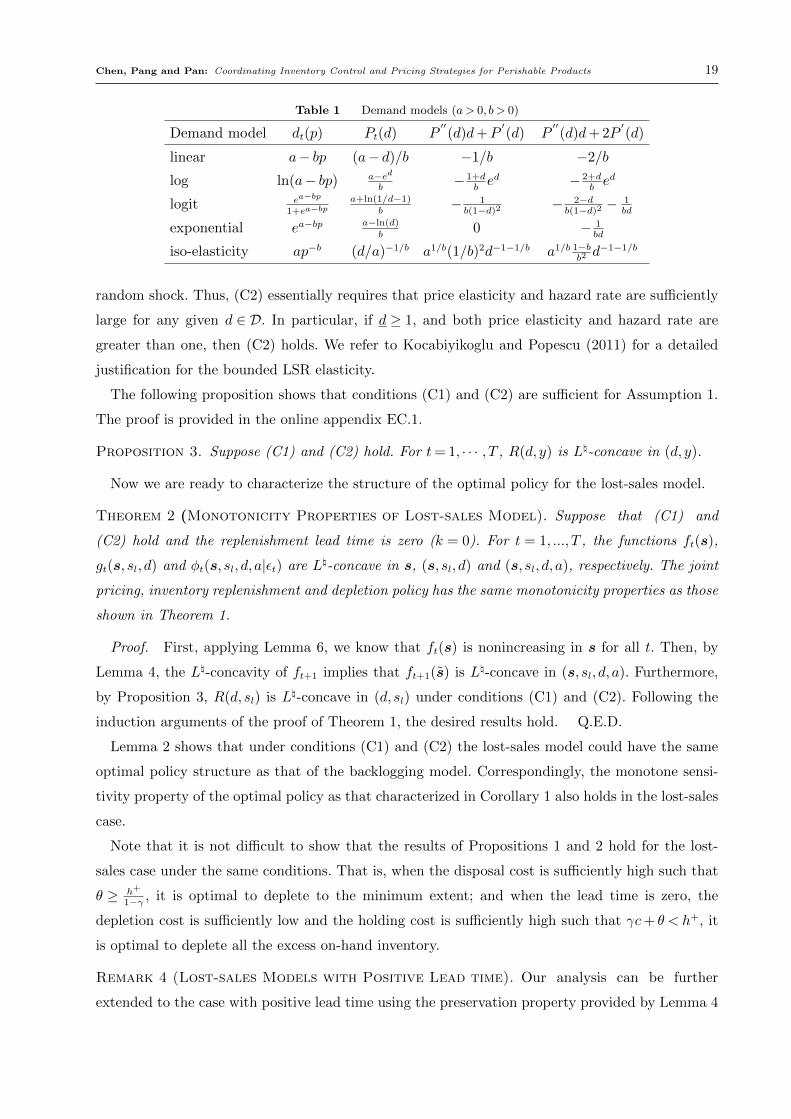
Chen, Pang and Pan: Coordinating Inventory Control and Pricing Strategies for Perishable Products 19
Table 1 Demand models (a> 0, b > 0)
Demand model dt(p) Pt(d) P′′(d)d+P
′(d) P
′′(d)d+ 2P
′(d)
linear a− bp (a− d)/b −1/b −2/b
log ln(a− bp) a−edb
− 1+dbed − 2+d
bed
logit ea−bp
1+ea−bpa+ln(1/d−1)
b− 1b(1−d)2
− 2−db(1−d)2
− 1bd
exponential ea−bp a−ln(d)
b0 − 1
bd
iso-elasticity ap−b (d/a)−1/b a1/b(1/b)2d−1−1/b a1/b 1−bb2d−1−1/b
random shock. Thus, (C2) essentially requires that price elasticity and hazard rate are sufficiently
large for any given d ∈ D. In particular, if d ≥ 1, and both price elasticity and hazard rate are
greater than one, then (C2) holds. We refer to Kocabiyikoglu and Popescu (2011) for a detailed
justification for the bounded LSR elasticity.
The following proposition shows that conditions (C1) and (C2) are sufficient for Assumption 1.
The proof is provided in the online appendix EC.1.
Proposition 3. Suppose (C1) and (C2) hold. For t= 1, · · · , T , R(d, y) is L\-concave in (d, y).
Now we are ready to characterize the structure of the optimal policy for the lost-sales model.
Theorem 2 (Monotonicity Properties of Lost-sales Model). Suppose that (C1) and
(C2) hold and the replenishment lead time is zero (k = 0). For t = 1, ..., T , the functions ft(s),
gt(s, sl, d) and φt(s, sl, d, a|εt) are L\-concave in s, (s, sl, d) and (s, sl, d, a), respectively. The joint
pricing, inventory replenishment and depletion policy has the same monotonicity properties as those
shown in Theorem 1.
Proof. First, applying Lemma 6, we know that ft(s) is nonincreasing in s for all t. Then, by
Lemma 4, the L\-concavity of ft+1 implies that ft+1(s) is L\-concave in (s, sl, d, a). Furthermore,
by Proposition 3, R(d, sl) is L\-concave in (d, sl) under conditions (C1) and (C2). Following the
induction arguments of the proof of Theorem 1, the desired results hold. Q.E.D.
Lemma 2 shows that under conditions (C1) and (C2) the lost-sales model could have the same
optimal policy structure as that of the backlogging model. Correspondingly, the monotone sensi-
tivity property of the optimal policy as that characterized in Corollary 1 also holds in the lost-sales
case.
Note that it is not difficult to show that the results of Propositions 1 and 2 hold for the lost-
sales case under the same conditions. That is, when the disposal cost is sufficiently high such that
θ ≥ h+
1−γ , it is optimal to deplete to the minimum extent; and when the lead time is zero, the
depletion cost is sufficiently low and the holding cost is sufficiently high such that γc+ θ < h+, it
is optimal to deplete all the excess on-hand inventory.
Remark 4 (Lost-sales Models with Positive Lead time). Our analysis can be further
extended to the case with positive lead time using the preservation property provided by Lemma 4

20 Chen, Pang and Pan: Coordinating Inventory Control and Pricing Strategies for Perishable Products
or Lemma 5. To this end, some monotone structural properties are required. We identify a sufficient
condition which helps us construct a monotone function to prove the preservation of L\-concavity
and the corresponding monotonicity properties of the optimal policies using Lemma 4. The detailed
analysis is presented in the last section of the online appendix EC.2.
Remark 5 (Depleting Decision Made Before Demand Is Realized). So far we assume
that the depleting decision is made after demand is realized. It may also be interesting to consider
the case that the depleting decision is made before demand is realized which at least can provide
a lower bound to the profit function of the lost-sales model studied above. Let a be the amount
of inventory to be depleted that is determined jointly with pricing and replenishment decisions at
the beginning of a period. Assume that s1 ≤ a≤ sl−k. If a is greater than the demand, a−dt units
of inventory are disposed of. Otherwise, dt− a units of demand are lost. The amount of inventory
to be carried over to the next period is sl−k − a. Then, the recursive optimality equation can be
written as
ft(s) = maxsl≥sl−1,d∈Dt,s1≤a≤sl−k
{R(d,a)−h+(sl−k− a)−h−E[(dt− a)+]− θE[(a− dt)+]
−c(sl− sl−1) + γft+1[(s2− a)+, (s3− a)+, ..., (sl−k− a)+, sl−k+1− a, ..., sl− a]}.
Using the following facts: (1) R(d,a) is L\-concave under conditions (C1) and (C2), (2) all the
other cost-related terms are L\-concave, (3) if ft+1 is L\-concave and decreasing in s1, ..., sl−k−1,
then the last term is also L\-concave, and (4) the constraint set forms an L\-convex set, we can
show that ft(s) is L\-concave and decreasing in s1, ..., sl−k−1, and the optimal policy structure is
similar to that characterized by Theorem 1.
6. Bounds, Heuristics and Numerical Study
One of the most significant features of L\-convexity is that it ensures the local optimum to be
the global optimum and a steepest descent-type polynomial-time algorithm can be used to find
the optimal solution (Murota 2005). Nevertheless, the computation for the perishable model still
suffers from the curse of dimensionality. In this section, we first derive analytical bounds on the
optimal inventory and demand level decisions and propose a heuristic to the perishable inventory
management problem. We then perform a numerical study to assess the performance of the heuristic
policies against the optimal policy. We restrict our discussions to the case with zero lead time.
6.1. Bounds
We first find bounds on the optimal order-up-to levels. For simplicity, we assume that θ≥ h+/(1−γ)
which ensures that the inventory is always depleted to the minimum extent. This is in line with the
perishable inventory literature and it allows us to focus on the replenishment and pricing decisions.
Chen, Pang and Pan: Coordinating Inventory Control and Pricing Strategies for Perishable Products 21
When at = dt ∨ s1, we have
φt(s, sl, dt ∨ s1, d|εt) = γcsl−1− csl− θ(dt ∨ s1− dt)−h+(sl− dt ∨ s1)+−h−(dt ∨ s1− sl)+ + γft+1(s)
= vt(sl, dt)− θ(s1− dt)+ + γft+1(s),
where for the backlogging case
vt(sl, dt) =−(1− γ)csl− γcdt−h+(sl− dt)+−h−(dt− sl)+,
and for the lost-sales case
vt(sl, dt) =−csl− (h+− γc)(sl− dt)+−h−(dt− sl)+,
with θ= θ+ γc−h+.
Define
St(d) = arg maxsl≥0
{Πt(sl, d) =R(d, sl) +E[vt(sl, d+ εt)]},
and
St(d) = arg maxsl≥0
{Πt(sl, d) =R(d, sl) +E[vt(sl, d+ εt)]− γcsl−1
−(γh+ + γ2h+ + ...+ γl−2h+ + γl−1θ)E[(sl− dt)+]}.
Note that St(d) represents a myopic solution considering the expected disposal cost to the minimum
extent, whereas St(d) is a myopic solution assuming that all the excess inventory is intentionally
held until it expires l periods later. The next theorem shows that St(d) and St(d) provide upper and
lower bounds on the inventory decisions for any given d. Note that St(d) is the ordering decision
without taking into account the possible disposal and holding costs associated with the ordered
inventory, which encourages ordering more, while St(d) is obtained by charging the maximum
possible holding and disposal costs, which overly penalizes the ordering decision and hence leads
to a lower order quantity.
Theorem 3 (Bounds). Suppose that the starting inventory level of the planning horizon is zero.
For all t, for any given demand level d,
St(d)∨ sl−1 ≤ slt(s, d)≤ St(d)∨ sl−1.
Proof. We first prove the upper bound. To this end, consider two inventory decisions s′l > sl.
Let s and s′ be the corresponding starting states of period t+1. Note that Gt(s, sl, d) = Πt(sl, d)+
γE[ft+1(s)]. The monotonicity of ft+1 implies that
Gt(s, s′l, d)−Gt(s, sl, d) ≤ Πt(s
′l, d)−Πt(sl, d).
22 Chen, Pang and Pan: Coordinating Inventory Control and Pricing Strategies for Perishable Products
Thus, Πt(sl, d) increases in sl when Gt(s, sl, d) increases in sl. By the concavity of Πt(sl, d) and
Gt(s, sl, d) in sl, we know that slt(s, d)≤ St(d)∨ sl−1.
We next turn to the lower bound. Consider two inventory decisions s′l > sl. Let s and s′ be the
corresponding starting states of period t+ 1. At the beginning of period t+ 1, the state s′ has
δ= s′l−1− sl−1 more units of inventory of age 1 (or fewer units of backorders) than s does. Construct
a policy (for state s′) such that the δ units of excessive inventory (if exist) are intentionally held
until they expire at the end of period t+ l− 1, incurring holding costs in periods t+ 1, ..., t+ l− 2
and disposal cost in period t+ l−1, while the rest of the system is operated as if the starting state
of period t+ 1 were s. The total profit incurred by the policy from period t+1 to the end of the
planning horizon is exactly ft+1(s)− (h+ + γh+ + ...+ γt+l−3h+ + γt+1−2θ)δ. Thus
ft+1(s)− (h+ + γh+ + ...+ γt+l−3h+ + γt+1−2θ)δ≤ ft+1(s′),
which implies that
ft+1(s) + csl−1− (h+ + γh+ + ...+ γt+l−3h+ + γt+1−2θ)δ≤ ft+1(s′) + cs′l−1.
Therefore, we have
Gt(s, s′l, d)−Gt(s, sl, d)
≥ Πt(s′l, d)−Πt(sl, d)− γc(s′l−1− sl−1) + γ[−(h+ + γh+ + ...+ γt+l−3h+ + γt+1−2θ)δ]
= Πt(s′l, d)− Πt(sl, d),
which implies that Gt(s, sl, d) is increasing in sl as Πt(sl, d) increases in sl. Thus, slt(s, d)≥ St(d)∨
sl−1. The desired results hold. Q.E.D.
Remark 6. The preceding analysis is based on stationary model parameters and independent
and identically distributed demands. Thus, the bounds are in fact independent of time. When the
system is non-stationary, we still have St(d)∨ sl−1 ≤ slt(s, d)≤ St(d)∨ sl−1, where St and St are
both time-dependent.
6.2. Heuristics
We now develop a one-dimensional approximation where the expected disposal cost associated with
each order is discounted to the period the order is placed. Since the future demand depends on the
future prices, we need to approximate the future demand levels or pricing decisions.
Federgruen and Heching (2002) point out that the optimal price path can be closely approximated
by the optimal price path under deterministic models. Using this observation, we approximate
the expected demand levels (and the corresponding prices) in the future periods with the optimal
demand levels derived from the corresponding deterministic models, which are also called the
Chen, Pang and Pan: Coordinating Inventory Control and Pricing Strategies for Perishable Products 23
optimal risk-less prices. That is, in any period t, the demand levels of next l − 1 periods are
approximated by dt+i, i= 1, ..., l− 1 where
dt+i = arg maxd∈D
{(Pt+i(d)− c)d}.
The corresponding demands are therefore approximated by dt+i + εt+i, i= 1, ..., l− 1
Let x and y be the inventory levels before and after ordering. Define
Bt(y, d) =E
(y− d− dt+1− ...− dt+l−1−l−1∑i=0
εt+i
)+ .
Given the demand approximation developed above, the expected amount of inventory to be dis-
posed of at the end of period t+ l− 1, denoted by Ot(x, y, d) satisfies
Bt(y−x,d)≤Ot(x, y, d)≤Bt(y, d)−Bt(x,d)≤Bt(y, d).
The expected disposal can be approximated by its upper bound Bt(y, d). That is, all the inventory
after ordering is treated as new inventory that can serve the demand in the next l−1 periods. Then,
the optimality equations for the approximate model can be expressed by the following: Starting
from vT+1(x) = 0,
vt(x) = maxy≥x,d∈D
Gt(y, d) (12)
where
Gt(y, d) = Πt(y, d)− γl−1θBt(y, d) + γE[vt+1(yt)].
For the backlogging case, yt = y− d− εt. For the lost sales case, y= (y− d− εt)+
Using the standard induction argument and applying Assumption 1, one can easily show that
Gt(y, d) is jointly concave and supermodular in (y, d) and ft preserves the nonincreasing and concave
properties. Therefore, the base-stock/list-price policy is optimal.
When the system is stationary, one may expect that the optimal price is stable as well. Thus, we
can use the current demand level to approximate the future demand levels, i.e., dt+i = d+ εt, i=
1, ..., l − 1 where d is the current demand level (see, e.g., Federgruen and Heching 1999). Then,
expected inventory disposal can be replaced by
Bt(y, d) =E
(y− l× d− l−1∑i=0
εt+i
)+ .
Using this approximation, one can show that a myopic base-stock list-price policy is optimal for
the stationary approximate model and the optimal solution is obtained by solving the following
problem:
maxy≥x,d∈D
{Πt(y, d)− γl−1θBt(y, d)
}. (13)
24 Chen, Pang and Pan: Coordinating Inventory Control and Pricing Strategies for Perishable Products
For convenience, we call the above heuristic policy H1. It is easy to show that for any given d, the
optimal order-up-to level, denoted by yH1(d), is in [St, St].
Li et al. (2009) follow Nahmias (1976) to approximate the expected disposal with a tighter upper
bound: Bt(y, d)−Bt(x,d). They suggest a myopic stationary policy by solving
maxy≥x,d∈D
{Πt(y, d)− γl−1θ[Bt(y, d)−E[Bt(y− d− εt, d)]]
}. (14)
We call this heuristic policy H2. It is easy to show that for any given d the optimal order-up-to
level of H2, denoted by yH2(d), is greater than yH1(d). It is notable that if we use Bt(y, d)−Bt(x,d)
to approximate the expected disposal (to replace Bt(y, d) in (12) by Bt(y, d)−Bt(x,d)) then the
base-stock list-price policy is not optimal (since the optimal order up to level must be dependent
on the inventory level). This is why we choose to approximate the disposal cost by Bt(y, d).
6.3. Numerical Study
Our numerical study aims to evaluate the performance of the heuristics in comparison with that of
optimal policies and assess the value of dynamic pricing in both infinite-horizon and finite-horizon
settings. The study is restricted to the backlogging cases with zero lead time. It is notable that
although the preceding analysis is focused on finite-horizon settings, the results can be readily
extended to infinite-horizon settings.
In the following numerical study, we first consider an infinite-horizon setting under the long-run
average profit criterion. Compared to the total expected discounted profit criterion, the long-
run average profit criterion provides a single performance indicator (i.e., long-run average profit)
which is independent of the initial system states and is therefore commonly used in the literature
to compare the performance of different policies. We then consider a finite-horizon setting with
both stationary and nonstationary demands. To compare the performance of different policies, the
performance indicator is chosen as the total expected discounted profits over the planning horizon
with a common starting state at zero. Finally, we examine the performance of the heuristics for
cost-minimization problems under the long-run average cost criterion. For simplicity, we require
that only the expired inventory is disposed of under different policies. Note that such a treatment
is optimal under the discounted profit criterion when θ≥ h+/(1− γ). Under the long-run average
profit (or cost) criterion, although it may be optimal to dispose of some inventory that is yet to
expire at some states, our numerical study shows that the impact of such a restriction on the
long-run average profits (or costs) is negligible for the instances we analyze.
6.3.1. Infinite-Horizon Setting We first compare the performance of different policies under
the infinite-horizon setting with the long-run average profit criterion.
Following Li et al. (2009), we adopt the test case parameters from Federgruen and Heching (1999).
The demand function is specified as an additive linear model dt = α−βp+ εt, where p∈ [p, p], and

Chen, Pang and Pan: Coordinating Inventory Control and Pricing Strategies for Perishable Products 25
εt follows a truncated normal distribution with zero mean and satisfies the nonnegativity condition
α−βp+ εt ≥ 0. The expected demand level is chosen from [d, d], where d= α−βp and d= α−βp.
Note that an up-tail truncated normal distribution has a positive mean σ φ(A/σ)
1−Φ(A/σ)for any given
truncating point A, where Φ and φ are standard normal distribution and density functions. For
the normally distributed random variable Z with zero mean and standard deviation σ, we find
the smallest point a≥−d such that A− σ φ(A/σ)
1−Φ(A/σ)≥−d. Let εt = {Z|Z ≥A} − σ φ(A/σ)
1−Φ(A/σ), where
{Z|Z ≥A} represents the up-tail truncation of Z from A. Clearly, εt has a zero mean and satisfies
the inequality εt ≥−d, which ensures the nonnegativity condition of the demand.
The system parameters are specified as follows. Three lifetimes are considered: l = 2,3,4. For
any l, we first set the base case as
[α,β, c.v., θ, c, h+, h−, p, p] = [174,3,1,10,22.15,0.22,10.78,25,44].
We then vary the parameters c.v., h− and θ, respectively, such that c.v. ∈ {0.6,0.8,1.0,1.2,1.5},
h− ∈ {1.98,4.18,10.78,21.78} (correspondingly, h−/(h− + h+) ∈ {90%,95%,98%,99%}), and θ ∈
{5,10,20}. In total, 33 instances are reported.
For each instance, we compute the optimal policy, the fixed-price policy and the heuristic policies
H1 and H2, and the corresponding long-run average profits. In particular, when computing the
fixed-price policy, we first compute the inventory policy for each given expected demand level d,
and then find the optimal demand level that leads to the maximum average profit.
The system state is discretized with step size 1. We apply the standard value iteration approach
to compute the long-run average profit per period and the optimal policies. The value iteration
algorithm is terminated when three-digit accuracy is obtained. See Bertsekas (1995) for the detailed
introduction to the value iteration approach under the long-run average cost or reward criterion.
When computing the optimal policies, for each iteration, given any state, we conduct linear search
for the optimal order-up-to level and the demand level. It is worthwhile to mention that the
properties of L\-concavity allow us to further reduce the search space. In particular, L\-concavity
ensures that the local optimum is globally optimal and the steepest accent method can be used
(instead of searching the whole decision space). The monotonicity properties of the state-dependent
policies ensure that the optimal solutions of smaller state can serve as lower bounds of the solutions
of larger states, which helps further reduce the computational effort.
Let dFP be the optimal expected demand level under fixe-price policy, and (sHil , dHi) be the opti-
mal myopic base stock and demand levels under the heuristic policy Hi, i= 1,2. The performance
of different policies is measured by the percentage profit loss ρu = V ∗−V u
V ∗ ×100%, u∈ {FP, H1, H2},
where V ∗, V FP , V H1 and V H2 are the long-run average profits under the optimal policy, fixed-
price policy, H1 and H2 heuristics, respectively. To gain insight into the role of dynamic pricing
in reducing the wastes arising from the disposals, we also compute the average disposal costs per
26 Chen, Pang and Pan: Coordinating Inventory Control and Pricing Strategies for Perishable Products
period under different policies, denoted by DCu, u∈ {∗,FP, H1, H2}. The percentage of the average
disposal cost in the average profit under policy u is denoted by δu = DCu
V u × 100%.
Table EC.1 below reports the performance of the optimal, fixed-price and heuristic policies,
and the corresponding static policy parameters for the 33 instances, indexed from 1 to 33. Table
EC.2 reports the corresponding disposal costs and their percentage ratios in profits. For ease of
reading, we use ‘-’ to represent the same value of the corresponding parameter in the base case.
The observations are summarized as follows.
• Table EC.1 shows that the long-run average profit under the optimal policy decreases in the
coefficient of variation, the unit backlogging cost, and the unit disposal cost, respectively, while
it increases in the product lifetime. The percentage profit losses of the fixed-price policy and the
heuristics have the same monotone patterns as the optimal policy, which implies that dynamic
pricing policy becomes more advantageous to the fixed-price policy and the heuristics when the
coefficient of variation, the unit backlogging, or the unit disposal cost becomes larger. In the
extreme case when the lifetime is infinite, our model reduces to the durable inventory model and
the heuristic policies become the optimal base-stock list-price policies (see, e.g., Federgruen and
Heching 1999). A natural conjecture arising from these observations is that when the lifetime
becomes sufficiently long, the performance of fixed-price and heuristic policies will converge to that
of the optimal policy.
• The heuristic policies H1 and H2 perform pretty well against the optimal policy. The per-
centage profit losses of most of the instances are below 1%, which is in line with the observations
of Li et al. (2009). In particular, when the lifetime is 4 periods and the coefficient of variation is
0.6, the percentage profit losses of heuristics are only 0.01%. Comparing the two heuristics, the
average profits and the optimal policy parameters (when taking integer values) are the same for
most instances with only a few exceptions (e.g., instances 3, 8, 9) in which H2 performs slightly
better than H1.
• The expected demand levels under the fixed-price policy or the heuristics tend to be smaller
as the lifetime increases. On the other hand, the order-up-to levels under H1 and H2 policies tend
to be larger as the lifetime increases. This implies that the retailer should offer lower prices and
order less when the product lifetime is shorter. That is, perishability reduces profit margins and
service levels.
• Table EC.2 compares the average disposals under different policies. One can observe that
both the average disposal cost and the percentage of the disposal cost in profit under the optimal
policy are lower than that under the fixed-price policy, which implies that dynamic pricing indeed
reduces the disposal wastes. The heuristic policies yield lower average disposal costs than those of
the optimal policy and fixed-price policy for most of the instances. For all the policies, it appears
that both the average disposal cost and the percentage of the disposal cost in profit increase in
Chen, Pang and Pan: Coordinating Inventory Control and Pricing Strategies for Perishable Products 27
the coefficient of variation, the backlogging cost, and the unit disposal cost. But when the lifetime
increases the average disposal cost decreases. This is because the likelihood to dispose of the
inventory becomes smaller when the product lifetime becomes longer.
• It is also worthwhile to mention that when the lifetime becomes longer the time to compute
the optimal policy increases exponentially. For example, for the base cases with l = 2,3,4, the
computing times for the optimal policies are 5 seconds, 283 seconds and 28 minutes, respectively,
using Matlab 7.0 on a personal computer with an Intel Core Duo 3.00GHz CPU.
In summary, these numerical results show that in the infinite-horizon setting, both the heuristics
perform very well. The errors of the approximations are ignorable in comparison with the possible
errors in calibrating the price-responsive demand functions.
6.3.2. Finite-Horizon Setting We next examine the performance of the heuristic policy H1
in a finite-horizon setting with nonstationary demand. Note that under H1 the base-stock/list-price
policy is optimal and the optimal policy parameters can be obtained by solving the optimality
equations (12).
Specifically, we consider a five-period horizon, T = 5. The time-varying demand functions are
specified as dt = κtα− βp, t= 1, ...,5, where κt is a time-varying seasonality factor such that κt =
1.2− 0.1× (t− 1), i.e., the market size falls over time from 1.2α to 0.8α with a slope of 0.1α. This
slope indicates how fast the demand falls over time. The smaller the slope, the more stable the
demand process. The average market size per period is α.
With all the other parameters being equal to those in the infinite-horizon setting, we vary c.v., h−
and θ, respectively. As the discounted profits are state-dependent, for the purpose of comparison,
we assume that the decision criterion is to maximize the total discounted profit over the planning
horizon with the initial inventory level being zero, denoted by the l-dimensional vector 0. The
discount factor is γ = 0.95. Clearly, for all the tested instances, we have θ > h+/(1− γ), which
ensures that it is optimal to only dispose of the expired inventory at the end of each period.
Similar to the infinite-horizon setting, the performance indicators of the heuristic policies can
be defined as the percentage profit losses at the common starting state 0,
ρu =ft(0)− fut (0)
ft(0)× 100%, u∈ {FP,H1},
where ft, fFPt and fH1
t are the discounted profit-to-go functions under the optimal, fixed-price,
and heuristic policies respectively. Let DC∗,DCFP and DCH1 be the corresponding discounted
disposal costs with the starting state 0 under different policies.
The numerical results are reported in Table EC.3. To examine the effect of demand variability
on the value of dynamic pricing, we further consider two scenarios: (1) the market size falls from
1.1α to 0.9α with a slope 0.05α while keeping the average market size per period at α, and (2)
the market size remains constant at α. The corresponding percentage profit losses under the FP

28 Chen, Pang and Pan: Coordinating Inventory Control and Pricing Strategies for Perishable Products
policy are denoted by ρFPI and ρFPII respectively. They are presented in the last two columns of
Table EC.3. We have the following observations.
• Consistent with the observations in the infinite-horizon setting, the discounted profit of the
optimal policy decreases in the coefficient of variation, the unit backlogging cost, and the unit dis-
posal cost respectively while it increases in the product lifetime. The magnitudes of the discounted
disposal costs in the finite-horizon setting with nonstationary demand are much larger than those
in the infinite-horizon setting.
• For the fixed-price policy, as the coefficient of variation, the unit backlogging cost, or the
unit disposal cost increases, or the lifetime becomes shorter, the performance becomes worse (i.e.,
dynamic pricing becomes more valuable) and the discounted disposal cost becomes larger. The
magnitudes of the percentage losses and the increased disposal costs (against the optimal policy)
are much larger than those in the infinite-horizon setting. This implies that the value of dynamic
pricing and its role in reducing wastes are much more significant when the demand is nonstationary.
• For the H1 heuristic policy, the percentage profit loss and the discounted disposal cost also
increase in the unit backlogging cost, or the unit disposal cost, and decreases in the lifetime. But,
when coefficient of variation increases the percentage profit loss of H1 becomes smaller. That is,
in the finite-horizon setting with nonstationary demand, H1 may perform better as the demand
variation increases, which is different from the infinite-horizon setting.
• When the slope of the seasonality factor κt falls from 0.1 to 0 while keeping the average market
size per period at α, the percentage profit losses fall quickly; see columns ρFP , ρFPI and ρFPII . As
a smaller slope implies a more stationary demand process and a smaller the percentage profit loss
implies a higher value of dynamic pricing, our results imply that the more variable the demand
process, the higher the value of dynamic pricing.
In summary, the value of dynamic pricing becomes much more significant in the finite-horizon
setting with nonstationary demand. Compared with the fixed-price policy, the heuristic policy H1
still performs well while keeping a simple policy structure.
6.3.3. Performance of Heuristics for Cost-Minimization Problems We now evaluate
the performance of the heuristic policies for the cost minimization problem with only replenishment
decisions. We restrict our study to the infinite-horizon setting with the long-run average cost as
the decision criterion, ignoring the revenue term Pt(d)d. The expected demand level, which is
exogenously given, is set as d= 54. For consistency, we still call the optimal policy with the fixed
expected demand level the optimal fixed-price policy. All the other parameters are the same as
those of the above numerical examples in the stationary setting.
The results are reported in Table EC.4 where Cu and DCu denote the long-run average cost
under policy u, u ∈ {FP,H1,H2}, and ρu = Cu−CFP
CFP × 100% denote the percentage cost increase
of the heuristic policy u∈ {H1,H2} against the FP policy.

Chen, Pang and Pan: Coordinating Inventory Control and Pricing Strategies for Perishable Products 29
From Table EC.4, we can observe that the percentage cost increases of the heuristics are less
than one percent for all the instances. Recall that the percentage profit losses of the heuristics
in Table EC.1 could be greater than 3%. This suggests that the heuristics perform better when
there are no pricing decisions and the revenue effects are removed. The sensitivity of the costs and
relative performance with respect to the system parameters are similar to those in Table EC.1
and Table EC.2. But the average disposal costs of the cost-minimization problems are consistently
higher than those in Table EC.2, which implies that the optimization of the pricing decisions can
indeed reduce the disposal costs. The order-up-to levels under H1 are slightly lower than that under
H2 and the performance of H2 is slightly better, which implies that under H1 the replenishment
decisions may be more conservative.
7. Concluding Remark
In this paper, we address a joint pricing and inventory control problem for stochastic perishable
inventory systems with positive lead time. Both the backlogging and lost-sales cases are studied.
We employ the concept of L\-convexity and develop new preservation properties to show some
monotonicity properties of the optimal policies. Unlike previous work which uses a sequence of
models with continuous demand distributions to approximate the discrete demand distributions,
our analysis allows for both continuous and discrete decision variables and thus provides a unified
approach to deal with models with both continuous and discrete demand distributions. We also
develop analytical bounds and propose a heuristic policy. Numerical study shows that the heuristic
policy performs very well. Finally, we show that our analysis can be further extended to the case
with random lifetime and the inventory rationing model with multiple demand classes.
Our models assume that inventories of any age can be disposed of purposely and customers are
not sensitive to the ages of inventories, which ensures that FIFO inventory issuing rule is optimal.
The FIFO assumption is particularly applicable to the contexts where organizations (e.g., online
retailers, blood banks and pharmacies) themselves fully control which inventory units are used to
meet the demand. Nevertheless, there are contexts in which other inventory issuing policies are
more plausible. For example, when customers are very sensitive to the ages of inventories (e.g., a
self-service grocery store where customers can make choices among units of different ages on the
same shelf) or when the freshest units are committed to be supplied first (e.g., some blood centres
and hospitals may have such service level agreements, Nahmias 2011), the last-in-first-out (LIFO)
inventory issuing policy is appropriate. When different prices are charged for inventories of different
ages, it is then critical to model the consumer choice behavior. Taking into account these issues in
perishable inventory models remains a significant challenge which deserves further exploration.
AcknowledgmentsWe thank the anonymous associate editor and two referees, Paul Zipkin and Yi Yang for their valuable comments on this
paper. This research was initiated while the first two authors were visiting the International Center of Management Science
30 Chen, Pang and Pan: Coordinating Inventory Control and Pricing Strategies for Perishable Products
and Engineering in Nanjing University. This research of the first author is partially supported by National Science Foundation
Grants CMMI-0926845 ARRA and CMMI-1030923 and National Science Foundation of China Grant 71228203.
References
The American Association of Blood Banks (AABB). 2009. The 2009 National Blood Collection and Uti-
lization Survey Report. Bethesda, Maryland, MD. http://www.aabb.org/programs/biovigilance/
nbcus/Documents/09-nbcus-report.pdf (accessed on March 18, 2013).
Bertsekas, D. P. 1995. Dynamic Programming and Optimal Control, Vol I, Athena Scientific, Belmont, MA.
Chan, L. M. A., Z. J. Max Shen, D. Simchi-Levi, J. Swann. 2004. Coordination of Pricing and Inven-
tory. Chapter 3 in Handbook of Quantitative Supply Chain Analysis: Modeling in the E-Business Era,
eds. D. Simchi-Levi, S. D. Wu and Z. J. Max Shen, Kluwer.
Chen, F. Y., S. Ray, Y. Song. 2006. Optimal pricing and inventory control policy in periodic-review systems
with fixed ordering cost and lost sales. Naval Res. Logist. 53(2) 117-136.
Chen, X., D. Simchi-Levi. 2004a. Coordinating inventory control and pricing strategies with random demand
and fixed ordering cost: The finite horizon case. Oper. Res. 52(6), 887-896.
Chen, X., D. Simchi-Levi. 2004b. Coordinating inventory control and pricing strategies with random demand
and fixed ordering cost: the infinite horizon case. Math. Oper. Res. 29(3), 698–723.
Chen, X., D. Simchi-Levi. 2006. Coordinating inventory control and pricing strategies with random demand
and fixed ordering cost: The continuous review model. Oper. Res. Lett. 34, 323–332.
Chen, X., D. Simchi-Levi. 2012. Pricing and inventory management. Oxford Hanbook of Pricing Management,
eds. Philips P and Ozer O, Oxford University Press, United Kingdom, pp. 784-822.
Elmaghraby, W., P. Keskinocak. 2003. Dynamic pricing in the presence of inventory considerations: research
overview, current practices, and future directions. Management Sci. 49 1287-1309.
Federgruen, A., A. Heching. 1999. Combined pricing and inventory control under uncertainty. Oper. Res.
47(3) 454–457.
Federgruen, A., A. Heching. 2002. Multilocation combined pricing and inventory control. Manuf. & Service
Oper. Management, 4(4) 275-295.
Ferguson, M. E., O. Koenigsberg. 2007. How should a firm manage deteriorating inventory? Production Oper.
Management 16(3) 306-321.
Food Market Institute. 2011. Supermarket sales by department - Percent of total supermarket sales. http:
//www.fmi.org/docs/facts-figures/grocerydept.pdf (accessed on Jan 20, 2012).
Fries, B. 1975. Optimal ordering policy for a perishable commodity with fixed lifetime. Oper. Res. 23(1)
46–61.
Huh, W. and G. Janakiraman. 2008. (s,S) optimality in joint inventory-pricing control: an alternate
approach. Oper. Res. 56 783-790.
Huh, W., G. Janakiraman. 2010. On the optimal policy structure in serial inventory systems with lost sales.
Oper. Res. 58(2) 481-491.
Chen, Pang and Pan: Coordinating Inventory Control and Pricing Strategies for Perishable Products 31
Li, Y., A. Lim, B. Rodrigues. 2009. Pricing and inventory control for a perishable product. Manufacturing
Service Oper. Mgmt. 11(3) 538-542.
Li, Y., B. Cheang, A. Lim. 2012. Grocery perishables management. Prod. and Oper. Magmt. 21(3) 504-517.
Kocabiyikoglu, A., I. Popescu. 2011. An elasticity perspective on the newsvendor with price sensitive demand.
Oper. Res. 59(2) 301–312.
Karaesmen, I. Z., A. Scheller-Wolf, B. Deniz. 2011. Managing perishable and aging inventories: Review and
future research directions. In: Kempf, K.G., Kskinocak P., Uzsoy P. (eds) Planning Production and
Inventories in The Extended Enterprise, Springer, Berlin, 393-436.
Lu, Y., J. S. Song. 2005. Order-based cost optimization in assemble-to-order systems. Oper. Res. 53(1)
151-169.
Murota, K. 2003. Discrete Convex Analysis. SIAM Monographs on Discrete Mathematics and Applications.
Society for Industrial and Applied Mathematics, Philadelphia, PA.
Murota, K. 2005. Note on multimodularity and L-convexity. Math. Oper. Res. 30(3) 658-661.
Murota, K. 2009. Recent developments in discrete convexity. In: W. Cook, L. Lovasz, J. Vygen (eds.) Recent
Developments in Combinatorial Optimization, Springer, 2009.
Nahmias, S. 1975. Optimal ordering policies for perishable inventory-II. Oper. Res. 23(4) 735-749.
Nahmias, S. 1976. Myopic approximations for the perishable inventory problem. Oper. Res. 24 1002–1008.
Nahmias, S. 1982. Perishable inventory theory: A review. Oper. Res. 23(4) 735-749.
Nahmias, S. 2011. Perishable Inventory Systems. International Series in Operations Research & Management
Sci., Vol. 160, Springer.
Nahmias, S., W.P. Pierskalla. 1973. Optimal ordering policies for a product that perishes in two periods
subject to stochastic demand. Naval Research Logistics Quarterly 20 207-229.
Nahmias S, Schmidt C.P. 1986. An application of the theory of weak convergence to the dynamic perishable
inventory problem with discrete demand. Math. Oper. Res. 11 62–69.
The National Supermarket Research Group. 2006. 2005 Supermarket Shrinking Report. http://www.
securestoreadvantage.com/pdfs/Supermarket_Survey_Executive_Summary.pdf (assessed on Jan
20, 2012).
Pang, Z. 2011. Optimal dynamic pricing and inventory control with stock deterioration and partial backo-
rdering. Oper. Res. Lett. 39 375–379.
Pang, Z., F. Chen, Y. Feng. 2012. A note on the structure of joint inventory-pricing control with leadtimes.
Oper. Res. 60:581-587.
Petruzzi, N. C., M. Dada. 1999. Pricing and the newsvendor model: A review with extensions. Oper. Res.
30(4) 680–708.
Pierskalla, W. P. 2004. Supply chain management of blood banks. In: Brandeau M., Sainfort F., Pierskalla
W. P. (eds) Operations Research and Health Care - A Handbook of Methods and Applications, Kluwer
Academic Publishers, New York, 104–145.

32 Chen, Pang and Pan: Coordinating Inventory Control and Pricing Strategies for Perishable Products
Simchi-Levi, D., X. Chen, J. Bramel. 2014. The Logic of Logistics: Theory, Algorithms, and Applications for
Logistics Management (Third Edition), Springer-Verlag, New York.
Song, Y., S. Ray, T. Boyaci. 2009. Optimal dynamic joint inventory-pricing control for multiplicative demand
with fixed order costs and lost sales. Oper. Res. 57(6) 245–250.
Webber, B., S. Herrlein, G. Hodge. 2011. Planet Retail: The Challenge of Food Waste. http://www-03.ibm.
com/press/uk/en/presskit/35447.wss (accssed on 8 September, 2012).
Xue, Z., M. Ettl, D. D. Yao. 2012. Managing freshness inventory: Optimal policy, bounds and heuristics.
Working paper, IBM T.J. Watson Research Center.
Yano, C. A., S. M. Gilbert. 2003. Coordinated pricing and production/procurement decisions: A
review, in Managing Business Interfaces: Marketing, Engineering and Manufacturing Perspectives, A.
Chakravarty, J. Eliashberg (eds.), Kluwer Academic Publishers, Boston, MA.
Zipkin, P. 2008. On the structure of lost-sales inventory models. Oper. Res. 56(4) 937-944.
Xin Chen is an associate professor of industrial engineering at the University of Illinois at Urbana-
Champaign. His research interests lie in supply chain management, revenue management, and optimization.
He received the INFORMS Revenue Management and Pricing Section Prize in 2009. He is the coauthor
of the book “The Logic of Logistics: Theory, Algorithms, and Applications for Logistics and Supply Chain
Management (Second Edition, 2005 & Third Edition, 2014)”.
Zhan Pang is a lecturer (assistant professor) of management science at Lancaster University Management
School. His research interests include supply chain management, pricing and revenue management, and risk
management.
Limeng Pan is a Ph.D. candidate of Systems and Entrepreneurial Engineering at the University of Illinois
at Urbana-Champaign. His research interests lie in dynamic systems with uncertainty, e.g., inventory control,
dynamic pricing and optimization.
e-companion to Chen, Pang and Pan: Coordinating Inventory Control and Pricing Strategies for Perishable Products ec1
E-companion to
“Coordinating Inventory Control and Pricing Strategies for
Perishable Products”Xin Chen
Department of Industrial and Enterprise Systems Engineering
University of Illinois at Urbana-Champaign, Urbana, IL 61801, [email protected]
Zhan Pang
Department of Management Science
Lancaster University, Lancaster LA1 4YX, United Kingdom, [email protected]
Limeng Pan
Department of Industrial and Enterprise Systems Engineering
University of Illinois at Urbana-Champaign, Urbana, IL 61801, [email protected]
This e-companion contains the technical proof of Theorem 3, two extensions, and four tables of
the numerical study.
EC.1. Proof of Theorem 3
It suffices to show that R(d− ζ, y− ζ) is supermodular in (d, y, ζ) for ζ ∈ {ζ : d− ζ ∈Dt,0≤ ζ ≤ y}.Note that R(d − ζ, y − ζ) = P (d − ζ)(d − ζ) + P (d − ζ)E[min(εt, y − d)]. Taking second-order
cross-partial derivatives with respect to (d, y) yields
∂2R
∂d∂y= P ′(d− ζ)F (y− d) +P (d− ζ)F ′(y− d) =−P ′(d− ζ)F (y− d)[%(d, y)− 1]≥ 0,
where the inequality is by condition (C2).
Taking second-order cross-partial derivatives with respect to (y, ζ) yields
∂2R
∂ζ∂y= −P ′(d− ζ)F (y− d)≥ 0,
where the inequality is due to P ′ < 0.
Taking second-order cross-partial derivatives with respect to (d, ζ) yields
∂2R
∂d∂ζ=−2P ′(d− ζ)−P
′′(d− ζ)(d− ζ)−P
′′(d− ζ)E[min(εt, y− d)] +P
′(d− ζ)F (y− d).
If P′′(d)≤ 0, then
∂2R
∂d∂ζ= −2P ′(d− ζ)−P
′′(d− ζ)E[min(d− ζ + εt, y− ζ)] +P
′(d− ζ)F (y− d)
≥ −2P ′(d− ζ) +P′(d− ζ)F (y− d)
≥ 0,

ec2 e-companion to Chen, Pang and Pan: Coordinating Inventory Control and Pricing Strategies for Perishable Products
where the first inequality is by the nonnegativity of E[min(d− ζ+ εt, y− ζ)] and the second by the
fact that −P ′(d− ζ) +P′(d− ζ)F (y− d) =−P ′(d− ζ)F (y− d)≥ 0 and P ′(d)≤ 0.
If, otherwise, P′′(d)> 0, then
∂2R
∂d∂ζ= −2P ′(d− ζ)−P
′′(d− ζ)(d− ζ)−P
′′(d− ζ)E[min(εt, y− d)] +P
′(d− ζ)F (y− d)
≥ −2P ′(d− ζ)−P′′(d− ζ)(d− ζ) +P
′(d− ζ)F (y− d)
≥ −[P ′(d− ζ) +P′′(d− ζ)(d− ζ)]
≥ 0,
where the first inequality is from E[min(εt, y− d)]≤E[εt] = 0, the second from P ′(d− ζ)≤ 0 and
the third from (C1). This completes the proof.
EC.2. Extensions
EC.2.1. Lost-Sales Model with Positive Lead Time
We now address the lost-sales model with positive lead time. Recall that in the lost-sales case
R(d, sl−k) = P (d)E[min(d+ εt, sl−k)] and
φt(s, sl, d, a|εt) =−(1− γ)csl− γca− θ(a− dt)−h+(sl−k− a)+− (h−− γc)(a− sl−k)+ + γft+1(s),
where
s= [(s2− a)+, ..., (sl−k− a)+, sl−k+1− a∧ sl−k, ..., sl− a∧ sl−k].
Note that the analysis for the lost-sales case with zero lead time relies on the monotonicity of
ft(s). However, when the lead time is positive (k≥ 1), the partial monotone structure of the profit
function under the dynamics (3) is not sufficient to ensure the preservation of L\-concavity. The
application of Lemma 5 requires that the underlying function to be monotone in all its components.
However, in the lost-sales case with positive lead time, the profit function ft may not always be
monotone in all its components. To show that L\-concavity can be preserved, we need to impose
the following sufficient condition.
(C3) h+ +h−− γc≥ γ(h−− γc+ p).
Condition (C3) states that the inventory cost incurring in the current period is greater than
the maximum potential benefit of carrying the inventory to the next period while holding on-hand
inventory and facing unmet demand simultaneously. This condition implies that it is always more
beneficial to meet the demand to the maximum extent. Note that the left-hand side of above
inequality does not take into account of the revenue (price) impact of inventory whereas the right-
hand side relaxes the price level to its upper bound, which implies that this condition can be
potentially further relaxed.
The next theorem shows that under conditions (C1)-(C3) the desired structural properties hold.

e-companion to Chen, Pang and Pan: Coordinating Inventory Control and Pricing Strategies for Perishable Products ec3
Theorem EC.1 (Monotonicity Properties of Optimal Policies). Suppose (C1)-(C3)
hold and k≥ 1. For t= 1, ..., T , the functions ft(s), gt(s, sl, d) and φt(s, sl, d, a|εt) are L\-concave in
s, (s, sl, d) and (s, sl, d, a), respectively. The joint pricing, inventory replenishment and depletion
policy has the same monotonicity properties as shown in Theorem 1.
Proof. The proof is by induction as the proof of Theorem 1. It suffices to show that
φt(s, sl, d, a|εt) is L\-concave in (s, sl, d, a) if ft+1 is L\-concave.
For any δ > 0, u > 0 and u+ δ ≤ a ∧ sl−k, comparing the system starting with state s = ((s2 −
u)+, ..., (sl−k − u)+, sl−k+1 − u, ..., sl − u) and the system with state s′ = ((s2 − u− δ)+, ..., (sl−k −
u− δ)+, sl−k+1 − u− δ, ..., sl − u− δ) at the beginning of period t+ 1, the latter has δ units less
on-hand inventory. Then, compared to the first system, the second system has at most δ units of
shortage in the following l− k− 1 periods, incurring at most δ units of lost sales, which implies
ft+1(s′)− ft+1(s)≥−(h−− γc+ p)δ.
Define ψt(s, sl, u) = (h+ +h−− γc)u+ γft+1(s). We have
ψt(s, sl, u+ δ)−ψt(s, sl, u)≥ δ[(h+ +h−− γc)− γ(h−− γc+ p)]≥ 0,
where the first inequality is from above analysis and the second is from (C3). That is, ψt(s, sl, u)
is monotone increasing in u, which implies that
ψt(s, sl, a∧ sl−k) = maxu≤a∧sl−k
ψt(s, sl, u).
By Lemma 6, we know that ft+1(s) is nonincreasing in (s1, ..., sl−k−1). Then, by Lemma 4, we
know that ft+1(s) is L\-concave in (s, sl, u). Clearly, φt(s, sl, u) is also L\-concave in (s, sl, u).
Note that the constraint set {u : 0 ≤ u ≤ a ∧ sl−k} forms a lattice. By Lemma 2, we know that
φt(s, a∧ sl−k) is L\-concave in (s, sl, a).
Note that (si− a)+ = (si− sl−k ∧ a)+ for all i < l− k. The dynamics of the system state can be
expressed as
s= [(s2− sl−k ∧ a)+, ..., (sl−k− sl−k ∧ a)+, sl−k+1− sl−k ∧ a, ..., sl− sl−k ∧ a],
Then, for any a≤ sl−k ∧ dt,
φt(s, sl, d, a|εt)
= −(1− γ)csl− γca− θ(a− dt)+−h+(sl−k− a)+− (h−− γc)(a− sl−k)+ + γft+1(s)
= −(1− γ)csl− γca− θ(a− dt)+−h+[sl−k− a∧ sl−k]− (h−− γc)[a− a∧ sl−k] + γft+1(s)
= −(1− γ)csl− γca− θ(a− dt)+−h+sl−k− (h−− γc)a+ψt(s, a∧ sl−k).
ec4 e-companion to Chen, Pang and Pan: Coordinating Inventory Control and Pricing Strategies for Perishable Products
Clearly, all the terms of the right-hand side of last equation are L\-concave. Thus, φt(s, sl, d, a|εt)
is L\-concave in (s, sl, a). It is clear that ft is L\-concave under conditions (C1) and (C2). By
induction, the desired structural results characterized in Theorem 1 hold. Q.E.D.
Theorem EC.1 shows that the desired structural properties could still hold in the lost-sales case
with positive lead time. Its proof shows that (C3) supplies some monotonicity to a transformed
profit-to-go functions, in addition to the partial monotonicity of the original profit-to-go function,
which allows us to apply Lemma 4.
Nevertheless, one may also be interested in applying Lemma 5, given the fact that the profit-to-
go function of the starting state of next period, ft+1(s), has the same form as that of the function
in Lemma 5. To this end, we need to impose new conditions under which some transformation
of the profit-to-go function is monotone. Note that the key tradeoff is between the lost-sales cost
and revenue in the future. It is possible to construct a transformed profit function with the lost-
sales cost when the lost-sales cost is high. We now present the idea without providing the proof:
Assume that (h−−γc)ρ≥ γθ+ p, where ρ= 1−γγ(1−γk)
. The transformed profit-go-to function ft(s) =
ft(s)−ρ(h−−γc)[sl−k +γsl−k+1 + ...+γk−1sl−1] is monotone decreasing in s. By Lemma 5, we can
show that L\-concavity can be preserved.
Remark EC.1 (Lost-Sales Inventory Models with Exogenous Price). When the price
p is exogenously given and constant over time, the model can be reduced to the standard lost-
sales perishable inventory model with the equivalent lost-sales cost h− + p. Then, condition (C3)
is replaced by (h+ +h−+p−γc)≥ γ(h−+p−γc), which holds automatically. Thus, our structural
analysis applies directly to the lost-sales perishable inventory model with positive leatimes, which
implies that our model generalizes Nahmias’ (2011) model to the case with positive lead time.
Remark EC.2 (Non-Stationary Lost-Sales Systems). Similar to the non-stationary back-
logging systems, our analysis can be easily extended to the non-stationary case under the conditions
θt ≥ γθt+1 and h+t +h−t − γct+1 ≥ γ(h−t+1− γct+2 + pt+1).
EC.2.2. Random Lifetime
We next extend our analysis to the case with random lifetime. For notational convenience, we
restrict our attention to the backlogging case with zero lead time.
As summarized by Nahmias (1977), the useful lifetime of many products (e.g., fresh produce,
meat, fowl, and fish) cannot be predicted in advance. Following Nahmias (1977), we assume that
the inventories outdate in the same order in which they enter the system. For each period t, let Kt
be a nonnegative integer random variable defined on the set {1,2, ..., l}. Assume that K1, ...,KT are
independent and identeically distributed. For a realization of Kt in period t, all on-hand inventory
that is at least Kt periods old at the end of period t will expire. Let πi = Pr(Kt = i). The dynamics
e-companion to Chen, Pang and Pan: Coordinating Inventory Control and Pricing Strategies for Perishable Products ec5
of the system state depend on the realization of Kt, denoted by s(i). Let a(i) be the inventory
depletion level when Kt = i such that a(i) ∈ [sl−i+1 ∨ dt, sl ∨ dt]. Then,
s(l) = (s2− a(l), s3− a(l), ..., sl−1− a(l), sl− a(l)),
s(l−1) = (0, s3− a(l−1), ..., sl−1− a(l−1), sl− a(l−1)),
...
s(1) = (0,0, ...,0,0).
Then, letting fT+1(s) = 0, the optimal profit-go-to function ft satisfies
ft(s) = maxsl≥sl−1,d∈Dt
R(d, sl) +E [gt(s, sl, d|εt)] ,
where
gt(s, sl, d|εt) = πl maxs1∨dt≤a(l)≤sl∨dt
{−vt(sl, a(l), dt) + γft+1(s(l))}
+ πl−1 maxs2∨dt≤a(l−1)≤sl∨dt
{−vt(sl, a(l−1), dt) + γft+1(s(l−1))}
...
+ π1[−vt(sl, sl ∨ dt, dt) + γft+1(0,0, ...,0,0)],
and
vt(sl, a, dt) = (1− γ)csl + γca+ θ(a− dt) +h+(sl− a)+ +h−(a− sl)+.
Analogous to the analysis in the proof of Theorem 1, one can show that ft is nondecreasing for
a(i) ≥ sl ∨ dt, the constraints a(i) ≤ sl ∨ dt are redundant, and the L\-concavity is preserved.
EC.2.3. Inventory Rationing with Multiple Demand Classes
Parallel to the pricing management, inventory rationing in the presence of multiple demand classes
is also an important strategy to leverage the supply and demand. Consider a lost-sales inventory
system with N classes of customers with different unit payments and lost-sales penalty costs.
Assume that the unit payments (prices) are fixed throughout the planning horizon. At the beginning
of each period, an order is placed and at the end of each period, after observing the realized
demands the system operator decides which customers’ demands to fulfill. In addition to satisfying
demands, we assume that the system operator can intentionally dispose of some aged inventory to
reduce the holding cost. The replenishment lead time of each order is of k periods.
Let n index the demand class. Let pn be the unit payment, h−n be the unit penalty cost for
class n, and dnt be the demand of class n in period t. Let dt = (d1t, ..., dNt). These demands could
be correlated in each period but they are independent across periods. Without loss of generality,
we assume that p1 + h−1 > p2 + h−2 > ... > pn + h−n , which implies that the class-1 demand has the
ec6 e-companion to Chen, Pang and Pan: Coordinating Inventory Control and Pricing Strategies for Perishable Products
highest priority, then the class-2, and so on. Denote by an the amount of inventory allocated to
class n’s demands, a0 the amount of additional inventory to be disposed of and a=∑N
n=0 an. Note
that 0≤ an ≤ dnt and s1 ≤ a≤ sl−k, the dynamics of the inventory are expressed as
s= ((s2− a)+, ..., (sl−k− a)+, sl−k+1− a, ..., sl− a).
Letting fT+1(s) = 0, the optimality equation can be expressed as:
ft(s) = maxsl≥sl−1
E[gt(s, sl|dt)], (EC.1)
where
gt(s, sl|dt)
= max0≤an≤dnt,s1≤
∑Nn=0 an≤sl−k
{R(a0, a1, ..., aN |dt)− (1− γ)csl− γc
N∑n=0
an−h+(sl−k−N∑n=0
an) + γft+1(s)
},
where
R(a0, a1, ..., aN |dt) =N∑n=1
pnan−N∑n=1
h−n (dnt− an)− θa0.
Clearly, for any given total amount allocation a, it is always optimal to meet the demands to
the maximum extent from the highest priority to the lowest priority and the payoff function
R(a1, ..., aN |dt) is entirely determined by a (see, e.g., Zipkin (2008) for a similar treatment). Let
R(a|dt) = max{R(a0, a1, ..., aN |dt)|0≤ an ≤ dnt,∑N
n=0 an = a}. It is clear that R(a|dt) is concave in
a. Then, we can represent gt as
gt(s, sl|dt) = maxs1≤a≤sl−k
{R(a|dt)− (1− γ)csl− γca−h+(sl−k− a) + γft+1(s)}.
Applying the previous analysis, we can show by induction that ft is nonincreasing in (s1, ..., sl−k−1).
By Lemma 4, ft+1(s) is L\-concave. Similar to preceding analysis, we can show that ft(s) is also
L\-concave. Hence the optimal inventory replenishment, rationing and disposal policy has a similar
structure to that characterized in Theorem 1.
Remark EC.3 (Backlogging Model with Multiple Demand Classes). Our analysis can
also be easily extended to the backlogging case with N demand classes. Let bn denote the number of
class-n backorders and h−n denote the unit backlogging cost per period. Assume that h−1 > .. > h−N .
Define z = (z1, ..., zN) where zn = b1 + ...+ bn represents the partial sum of backorders from class 1
to class n, n= 1, ...,N . Then the system state can be represented by (z, s). Again, let a be the total
amount of inventory to be depleted such that s1 ≤ a≤ sl−k. Let dnt = d1t + ...+ dnt be the partial
sum of demands from class 1 to class n. The dynamics of the system state can be expressed as
(z, s) = ((z1 + d1t− a)+, ..., (zN + dNt− a)+, s2− a, ..., sl− a). Let fT+1(z, s) = 0. The optimal value
functions satisfy the following optimality equations.
ft(z, s) = maxsl≥sl−1
E[gt(z, s, sl|dt)],
e-companion to Chen, Pang and Pan: Coordinating Inventory Control and Pricing Strategies for Perishable Products ec7
where
gt(z, s, sl|dt) = maxs1≤a≤sl−k
{R(a|dt,zt)− (1− γ)csl− γca−h+(sl−k− a)+ + γft+1(z, s)},
with R(a|dt,zt) =∑N
n=1 pndnt−∑N
n=1(h−n −h−n+1)(zn + dnt− a)+− θ(a− zN − dNt)+ and h−N+1 = 0.
Clearly, R(a,zt|dt) is L\-concave in (a,zt), and ft is decreasing in zn, n = 1, ...,N . By Lemma 4,
ft+1(z, s) is L\-concave. Similar to preceding analysis, we can obtain the desired results.
EC.3. Tables of Numerical Study
References
Nahmias, S. 1977. On ordering perishable inventory when both the demand and lifetime are random. Man-
agement Sci. 24 82–90.
Nahmias, S. 2011. Perishable Inventory Systems. International Series in Operations Research & Management
Sci., Vol. 160, Springer US.
Zipkin, P. 2008. On the structure of lost-sales inventory models. Oper. Res. 56(4) 937-944.
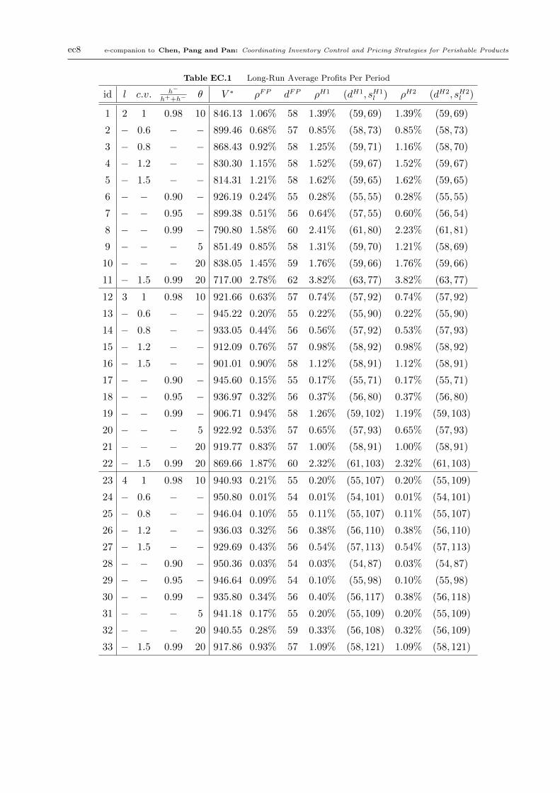
ec8 e-companion to Chen, Pang and Pan: Coordinating Inventory Control and Pricing Strategies for Perishable Products
Table EC.1 Long-Run Average Profits Per Period
id l c.v. h−
h++h− θ V ∗ ρFP dFP ρH1 (dH1, sH1l ) ρH2 (dH2, sH2
l )
1 2 1 0.98 10 846.13 1.06% 58 1.39% (59,69) 1.39% (59,69)
2 − 0.6 − − 899.46 0.68% 57 0.85% (58,73) 0.85% (58,73)
3 − 0.8 − − 868.43 0.92% 58 1.25% (59,71) 1.16% (58,70)
4 − 1.2 − − 830.30 1.15% 58 1.52% (59,67) 1.52% (59,67)
5 − 1.5 − − 814.31 1.21% 58 1.62% (59,65) 1.62% (59,65)
6 − − 0.90 − 926.19 0.24% 55 0.28% (55,55) 0.28% (55,55)
7 − − 0.95 − 899.38 0.51% 56 0.64% (57,55) 0.60% (56,54)
8 − − 0.99 − 790.80 1.58% 60 2.41% (61,80) 2.23% (61,81)
9 − − − 5 851.49 0.85% 58 1.31% (59,70) 1.21% (58,69)
10 − − − 20 838.05 1.45% 59 1.76% (59,66) 1.76% (59,66)
11 − 1.5 0.99 20 717.00 2.78% 62 3.82% (63,77) 3.82% (63,77)
12 3 1 0.98 10 921.66 0.63% 57 0.74% (57,92) 0.74% (57,92)
13 − 0.6 − − 945.22 0.20% 55 0.22% (55,90) 0.22% (55,90)
14 − 0.8 − − 933.05 0.44% 56 0.56% (57,92) 0.53% (57,93)
15 − 1.2 − − 912.09 0.76% 57 0.98% (58,92) 0.98% (58,92)
16 − 1.5 − − 901.01 0.90% 58 1.12% (58,91) 1.12% (58,91)
17 − − 0.90 − 945.60 0.15% 55 0.17% (55,71) 0.17% (55,71)
18 − − 0.95 − 936.97 0.32% 56 0.37% (56,80) 0.37% (56,80)
19 − − 0.99 − 906.71 0.94% 58 1.26% (59,102) 1.19% (59,103)
20 − − − 5 922.92 0.53% 57 0.65% (57,93) 0.65% (57,93)
21 − − − 20 919.77 0.83% 57 1.00% (58,91) 1.00% (58,91)
22 − 1.5 0.99 20 869.66 1.87% 60 2.32% (61,103) 2.32% (61,103)
23 4 1 0.98 10 940.93 0.21% 55 0.20% (55,107) 0.20% (55,109)
24 − 0.6 − − 950.80 0.01% 54 0.01% (54,101) 0.01% (54,101)
25 − 0.8 − − 946.04 0.10% 55 0.11% (55,107) 0.11% (55,107)
26 − 1.2 − − 936.03 0.32% 56 0.38% (56,110) 0.38% (56,110)
27 − 1.5 − − 929.69 0.43% 56 0.54% (57,113) 0.54% (57,113)
28 − − 0.90 − 950.36 0.03% 54 0.03% (54,87) 0.03% (54,87)
29 − − 0.95 − 946.64 0.09% 54 0.10% (55,98) 0.10% (55,98)
30 − − 0.99 − 935.80 0.34% 56 0.40% (56,117) 0.38% (56,118)
31 − − − 5 941.18 0.17% 55 0.20% (55,109) 0.20% (55,109)
32 − − − 20 940.55 0.28% 59 0.33% (56,108) 0.32% (56,109)
33 − 1.5 0.99 20 917.86 0.93% 57 1.09% (58,121) 1.09% (58,121)

e-companion to Chen, Pang and Pan: Coordinating Inventory Control and Pricing Strategies for Perishable Products ec9
Table EC.2 Average Disposal Costs Per Period
id l c.v. h−
h++h− θ DC∗ δ∗ DCFP δFP DCH1 δH1 DCH2 δH2
1 2 1 0.98 10 9.67 1.14% 13.24 1.58% 9.65 1.16% 9.65 1.16%
2 − 0.6 − − 6.60 0.73% 8.85 0.99% 7.04 0.79% 7.04 0.79%
3 − 0.8 − − 8.78 1.01% 11.66 1.36% 8.50 0.99% 9.23 1.08%
4 − 1.2 − − 10.16 1.22% 13.71 1.67% 9.80 1.20% 9.80 1.20%
5 − 1.5 − − 8.78 1.01% 11.66 1.36% 8.50 0.99% 9.23 1.08%
6 − − 0.90 − 1.50 0.16% 2.23 0.24% 1.57 0.17% 1.57 0.17%
7 − − 0.95 − 3.64 0.40% 5.33 0.60% 3.59 0.40% 4.04 0.45%
8 − − 0.99 − 17.74 2.24% 22.95 2.95% 16.24 2.10% 17.37 2.24%
9 − − − 5 5.99 0.70% 7.68 0.91% 5.23 0.62% 5.66 1.67%
10 − − − 20 13.62 1.63% 19.39 2.35% 14.87 1.81% 14.87 1.81%
11 − 1.5 0.99 20 28.18 3.93% 39.64 5.69% 27.10 3.93% 27.10 3.93%
12 3 1 0.98 10 2.30 0.25% 4.14 0.45% 3.26 0.36% 3.26 0.36%
13 − 0.6 − − 0.81 0.09% 1.53 0.16% 1.35 0.14% 1.35 0.14%
14 − 0.8 − − 1.63 0.17% 3.14 0.34% 2.11 0.23% 2.31 0.25%
15 − 1.2 − − 2.73 0.30% 5.04 0.56% 3.31 0.37% 3.31 0.37%
16 − 1.5 − − 3.07 0.34% 5.53 0.62% 3.89 0.44% 3.89 0.44%
17 − − 0.90 − 0.47 0.05% 0.86 0.09% 0.72 0.08% 0.72 0.08%
18 − − 0.95 − 1.05 0.11% 1.86 0.20% 1.42 0.15% 1.42 0.15%
19 − − 0.99 − 3.71 0.41% 6.80 0.76% 4.45 0.50% 4.79 0.53%
20 − − − 5 1.42 0.15% 2.38 0.26% 1.77 0.19% 1.77 0.19%
21 − − − 20 3.11 0.34% 6.97 0.76% 4.62 0.51% 4.62 0.51%
22 − 1.5 0.99 20 7.30 0.84% 14.87 1.74% 9.86 1.16% 9.86 1.16%
23 4 1 0.98 10 0.45 0.05% 1.14 0.12% 0.83 0.09% 0.91 0.10%
24 − 0.6 − − 0.05 0.01% 0.11 0.01% 0.11 0.01% 0.11 0.01%
25 − 0.8 − − 0.23 0.03% 0.52 0.05% 0.46 0.05% 0.46 0.05%
26 − 1.2 − − 0.65 0.07% 1.50 0.16% 1.10 0.12% 1.10 0.12%
27 − 1.5 − − 0.86 0.09% 2.11 0.23% 1.39 0.15% 1.39 0.15%
28 − − 0.90 − 0.07 0.01% 0.17 0.02% 0.15 0.02% 0.15 0.02%
29 − − 0.95 − 0.18 0.02% 0.49 0.05% 0.34 0.04% 0.34 0.04%
30 − − 0.99 − 0.75 0.08% 1.74 0.19% 1.38 0.15% 1.49 0.16%
31 − − − 5 0.27 0.03% 0.62 0.07% 0.50 0.05% 0.50 0.05%
32 − − − 20 0.63 0.07% 1.94 0.21% 1.27 0.14% 1.39 0.15%
33 − 1.5 0.99 20 1.99 0.22% 6.04 0.66% 3.84 0.42% 3.84 0.42%

ec10 e-companion to Chen, Pang and Pan: Coordinating Inventory Control and Pricing Strategies for Perishable Products
Table EC.3 Finite-Horizon Models with Non-Stationary Demand
id l c.v. h−
h++h− θ f1(0) DC∗ ρFP DCFP ρH1 DCH1 ρFPI ρFPII
1 2 1 0.98 10 4030.01 36.35 7.06% 52.83 5.25% 11.91 2.88% 1.14%
2 − 0.6 − − 4254.17 26.84 6.32% 39.32 13.10% 2.29 2.37% 0.65%
3 − 0.8 − − 4120.29 34.40 6.79% 48.46 10.21% 4.86 2.69% 0.96%
4 − 1.2 − − 3968.62 37.51 7.24% 54.21 0.92% 34.57 2.99% 1.26%
5 − 1.5 − − 3908.39 36.76 7.39% 53.83 0.35% 60.80 3.09% 1.35%
6 − − 0.90 − 4580.56 1.13 4.77% 1.52 0.44% 1.41 1.34% 0.02%
7 − − 0.95 − 4385.61 8.73 5.36% 13.07 1.81% 4.55 1.78% 0.26%
8 − − 0.99 − 3671.74 77.92 9.26% 107.76 8.72% 28.19 4.29% 2.43%
9 − − − 5 4050.30 22.43 6.82% 30.31 4.75% 6.83 2.67% 0.94%
10 − − − 20 399.49 51.30 7.51% 81.66 6.27% 19.48 3.26% 1.54%
11 − 1.5 0.99 20 3352.01 122.58 11.40% 186.14 2.81% 276.49 5.84% 4.27%
12 3 1 0.98 10 4275.98 7.95 6.37% 19.03 8.10% 0.08 2.10% 0.26%
13 − 0.6 − − 4419.89 3.71 5.49% 11.30 12.58% 0.01 1.55% 0.04%
14 − 0.8 − − 4338.89 6.52 6.05% 18.67 11.56% 0.03 1.86% 0.15%
15 − 1.2 − − 4228.68 8.91 6.57% 21.50 4.15% 0.39 2.27% 0.36%
16 − 1.5 − − 4178.09 9.45 6.67% 23.45 2.65% 0.64 2.38% 0.45%
17 − − 0.90 − 4591.46 0.13 4.76% 0.15 0.29% 0.00 1.32% 0.00%
18 − − 0.95 − 4460.42 1.78 5.11% 4.58 2.33% 0.02 1.45% 0.03%
19 − − 0.99 − 4112.85 16.89 7.70% 43.24 14.34% 0.32 2.75% 0.65%
20 − − − 5 4280.44 5.07 6.23% 10.51 7.47% 0.05 1.98% 0.21%
21 − − − 20 4269.36 10.96 6.62% 31.10 9.02% 0.15 2.30% 0.37%
22 − 1.5 0.99 20 3918.44 29.29 9.52% 78.71 3.73% 7.90 3.92% 1.57%
23 4 1 0.98 10 4340.39 1.22 5.76% 8.24 7.70% 0.00 1.54% 0.01%
24 − 0.6 − − 4445.33 0.25 5.09% 2.21 9.54% 0.00 1.37% 0.00%
25 − 0.8 − − 4387.17 0.77 5.46% 5.63 9.56% 0.00 1.45% 0.00%
26 − 1.2 − − 4303.57 1.58 5.98% 9.87 5.29% 0.00 1.62% 0.02%
27 − 1.5 − − 4262.57 1.90 6.21% 11.23 4.54% 0.00 1.73% 0.04%
28 − − 0.90 − 4592.30 0.00 4.76% 0.00 0.18% 0.00 1.32% 0.00%
29 − − 0.95 − 4475.38 0.14 4.96% 1.03 1.95% 0.00 1.36% 0.00%
30 − − 0.99 − 4237.33 3.01 6.77% 15.33 14.02% 0.00 1.86% 0.05%
31 − − − 5 4341.07 0.77 5.67% 4.57 7.29% 0.00 1.51% 0.01%
32 − − − 20 4339.40 1.62 5.91% 13.87 8.36% 0.00 1.59% 0.02%
33 − 1.5 0.99 20 4107.71 6.06 8.07% 33.36 7.73% 0.00 2.56% 0.26%

e-companion to Chen, Pang and Pan: Coordinating Inventory Control and Pricing Strategies for Perishable Products ec11
Table EC.4 Average Costs and Disposal Costs Per Period for Cost-Minimization Problems
id l c.v. h−
h++h− θ CFP DCFP ρH1 DCH1 sH1l ρH2 DCH2 sH2
l
1 2 1 0.98 10 1329.39 14.62 0.24% 11.32 61 0.24% 11.32 61
2 − 0.6 − − 1270.30 9.79 0.12% 8.34 67 0.12% 8.34 67
3 − 0.8 − − 1305.02 13.49 0.24% 10.00 63 0.17% 10.81 64
4 − 1.2 − − 1346.42 15.74 0.34% 10.64 58 0.26% 11.53 59
5 − 1.5 − − 1363.36 15.98 0.27% 11.58 57 0.27% 11.58 57
6 − − 0.90 − 1236.55 2.25 0.02% 1.84 44 0.02% 1.84 44
7 − − 0.95 − 1267.01 5.44 0.09% 4.04 50 0.09% 4.04 50
8 − − 0.99 − 1395.38 27.52 0.61% 19.72 69 0.48% 20.97 70
9 − − − 5 1321.39 8.80 0.32% 6.11 62 0.25% 6.58 63
10 − − − 20 1342.43 22.94 0.22% 17.74 57 0.22% 17.74 57
11 − 1.5 0.99 20 1484.95 49.12 0.71% 33.67 62 0.57% 36.04 63
12 3 1 0.98 10 1247.11 5.20 0.13% 3.82 85 0.13% 3.82 85
13 − 0.6 − − 1217.16 1.70 0.02% 1.48 88 0.02% 1.48 88
14 − 0.8 − − 1232.76 3.70 0.06% 2.97 87 0.06% 2.97 87
15 − 1.2 − − 1258.90 6.24 0.21% 4.22 83 0.16% 4.55 84
16 − 1.5 − − 1272.20 7.27 0.22% 4.93 82 0.17% 5.31 83
17 − − 0.90 − 1216.03 0.97 0.01% 0.81 69 0.01% 0.81 69
18 − − 0.95 − 1226.78 2.25 0.06% 1.58 75 0.04% 1.74 76
19 − − 0.99 − 1267.95 8.91 0.29% 6.32 92 0.22% 6.75 93
20 − − − 5 1244.36 2.97 0.15% 2.06 86 0.11% 2.23 87
21 − − − 20 1251.81 8.42 0.16% 6.00 82 0.12% 6.52 83
22 − 1.5 0.99 20 1320.79 21.60 0.51% 14.06 87 0.42% 15.02 88
23 4 1 0.98 10 1221.47 1.34 0.03% 0.99 105 0.03% 0.99 105
24 − 0.6 − − 1209.33 0.11 0.00% 0.11 101 0.00% 0.11 101
25 − 0.8 − − 1214.96 0.63 0.01% 0.50 104 0.01% 0.50 104
26 − 1.2 − − 1227.78 1.92 0.06% 1.41 105 0.04% 1.52 106
27 − 1.5 − − 1235.90 2.63 0.08% 1.92 105 0.08% 1.92 105
28 − − 0.90 − 1209.91 0.17 0.00% 0.17 88 0.00% 0.17 88
29 − − 0.95 − 1214.22 0.49 0.01% 0.38 95 0.01% 0.43 96
30 − − 0.99 − 1228.51 2.30 0.05% 1.87 113 0.05% 1.87 113
31 − − − 5 1220.78 0.72 0.03% 0.54 106 0.02% 0.59 107
32 − − − 20 1222.67 2.28 0.03% 1.82 104 0.03% 1.82 104
33 − 1.5 0.99 20 1255.48 8.03 0.20% 5.51 110 0.16% 5.90 111