In A. Artiba and S.E. Elmaghraby (eds.),The Planning and Scheduling of Production Systems: Methodologies and Applications,

London: Chapman and Hall, 1996.

Constraint Logic and Its Applications In Production:

An Implementation Using the Galileo4 Language and System∗

Dennis Bahlerbahler@ncsu.edu

Department of Computer ScienceNorth Carolina State University

Raleigh, NC 27695-8206 USA

and

James Bowenjabowen@jim.ucc.ie

Department of Computer ScienceNational University of Ireland

Cork, Ireland

February 1996

Abstract

The flexible and efficient support of the process of product design and production requirescombined expertise from many aspects of the product life-cycle, and the management and useof this knowledge in turn increasingly requires sophisticated computer-based advice systems. Inthis chapter we present a constraint-based approach to making the full First-Order PredicateCalculus available for knowledge representation purposes in intelligent networked colocationadvice systems for concurrent engineering. Domain knowledge is represented as a theory writtenin a first-order logical language. The set of models of the language under which the theory issatisfied is the set of solutions of a constraint network. Solutions to the network are computedby a hierarchical and opportunistic constraint inference method. Galileo4, an implementedlanguage and companion run-time system based on these ideas is discussed and its efficacy isdemonstrated by presenting applications in which high problem-solving versatility is providedby concise and readable programs.

1 Introduction

Concurrent engineering (CE) is an approach to the organization and management of design, pro-duction, marketing, etc. in which, in order to avoid costly downstream redesign, aspects of theproduct life cycle such as manufacturability, testability, repairability, and marketing are taken intoaccount as early in the design process as possible. Since most life-cycle costs are dictated in the

∗This work was partially supported by the National Science Foundation under Grants DDM-8914200 and DDM-9215755 and by IBM Corp.

1

design phase, it is important that life-cycle information be available to the designer so that it caninfluence product design. Once a product has completed the design stage, it is too late to makesignificant changes in life-cycle costs. The U.S. National Science Foundation, for example, hasestimated that 70% or more of a product’s manufacturing cost is dictated by design decisions.

Currently many companies attempt to implement concurrent engineering at the detailed designphase by maintaining checklists or rulebooks that a designer must adhere to and then schedulingface-to-face meetings with the appropriate experts at critical project points. In our interaction withcompanies we have found several problems with this approach. First, the rulebooks or checklistsare getting so large and complex that even the experts, let alone the designer, cannot help lettingdesign deficiencies through to manufacture. Second, the need for physical meetings reduces time-to-market. One way to overcome these difficulties is to use Networked Colocation. In thisapproach, the team members supplement face-to-face meetings with electronic communication overa computer network.

The concept of networked colocation can be realized with varying degrees of sophistication. Atits simplest, it may amount to no more than some combination of electronic mail and shared accessto a CAD database. However, something much more sophisticated is needed if we are to succeed inCE. Product development teams often find themselves overwhelmed by the volume and variety ofinformation that arises in CE. As the design evolves, the number of concerns grows quickly beyondwhat even a team of persons can successfully manage. We need software which can relieve someof this cognitive overload. What is needed is an Intelligent Networked Colocation Advisor(INCA) which not only relieves the logistic and scheduling difficulties but also reduces the problemcomplexity perceived by team members. These design advice tools are intended for use by and formultiple clients, including both computer systems and human users.

In our experience [3, 4, 5] constraint-based systems constitute a good basis for such tools;much of our effort has emphasized expressive competence in constraint-based languages in order toprovide a convenient and sufficient representation of the kind of real-world problems encounteredin concurrent engineering. Moreover, we believe that an approach to constraint processing whichis strongly grounded in a formal logical model offers the greatest chance to gain insight and makeprogress. Accordingly, we view a network of interlocking constraints as a collection of sentences inFirst-Order Predicate Calculus (FOPC). Constraint processing then becomes exactly the processof semantic modeling, that is, finding an interpretation for the symbols appearing in the theorythat renders the constraint sentences true according to some well defined measure of truth. In thisway the notions of constraint logic and constraint network are mutually intertwined.

The remainder of this chapter is organized as follows. In Section 2, we briefly present anoverview of Galileo4, the latest of a set of constraint programming languages and companion run-time systems we have developed for constructing INCAs, and illustrate the utility of this systemfor supporting a production task application in design for testability of printed wiring boards. InSection 3, we further illustrate the practical utility of the constraint-based approach by discussinganother application, this time in the realm of selecting lowest-cost insertion robot equipment whilefulfilling a set of user-supplied specifications. In Section 4, we compare our approach with otherconstraint-based techniques.

Beginning in Section 5, we elaborate in a more technical vein on the relationship between con-straint networks and semantic models in logic. In this view the consistency of a constraint networkcorresponds to the satisfiability of a theory in logic, and we argue that a suitable computationalapproach to the full FOPC can be based on generalizing the consistency algorithms [21] that havebeen presented in the literature on constraint satisfaction problems (CSPs). In Section 6, we lookat Galileo4 from a more formal perspective, using a progression of sample programs to illustratethe correspondence between constraint processing and semantic modeling. In Section 7, we discuss

2

human-machine interaction in Galileo4 in terms of a model of machine-interlocutor interaction.Finally, in Section 8, we make some concluding remarks.

2 The Utility of Constraint Processing for Production

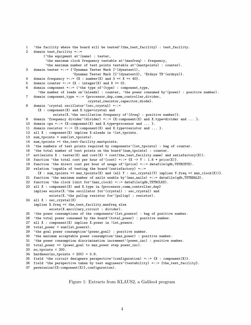
Galileo4 is a language and run-time system we have developed for the construction and use ofINCAs. In this section, we will consider a Galileo4 program called KLAUS2, which is an INCA forprinted wiring board design. In this section, we will consider only a few extracts from KLAUS2(Figure 1). For a more complete presentation of KLAUS2, see [4].

A program in Galileo4 specifies a frame-based constraint network and comprises a set of dec-larations and definitions. The declaration statements include declarations of the parameters thatexist in the network and the constraints that exist between these parameters. The definition state-ments include definitions for: partitions which divide the network into different regions that may beseen by different classes of user; application-specific domains, functions, and relations that are usedin constraint declarations; and icons for application-specific domains, if it is intended to presentcertain regions of the network to users graphically rather than textually, a textual presentationbeing the default.

In a Galileo4 program, statements can be written in any order, although good software engi-neering practice dictates that some agreed standard ordering be used, in order to facilitate programmaintenance. In Figure 1, we have taken advantage of this free-ordering by listing the statementsin an order which facilitates discussion in this chapter; in KLAUS2 itself, however, the statementsare ordered differently. Although the statements are numbered in Figure 1, this is purely for thepurposes of the current exposition; the numbers are not part of the program text. The discussionthat follows will be very dense, because of the need to illustrate many features of a richly expressivelanguage in a very short space. Reviewers wanting a more leisurely overview of the language areencouraged to read [4]. Galileo4 is a research prototype which is available on an as-is basis. Thecurrent version runs on IBM PS/2’s and compatible hardware.

Frame-based Product-Process-Organization Modeling: In a frame-based constraint net-work, frames can be used to represent a model of Product, Process, and Organization (PPO).Consider, for example, statement 1 of Figure 1 which declares the existence of a parameter calledthe test facility and specifies that it is of type, or domain, test facility. The string delim-ited by apostrophes is a long synonym which specifies the name by which the parameter will bereferenced in all output given to users of the program. From this, it can be seen that this parameterrepresents the facility where the board will be tested.

This parameter is a frame, as can be seen in statement 2, which defines the application-specificdomain test facility referenced in statement 1. The statement specifies that a test facility isrepresented by a frame containing three slots. For each slot, we specify its name, its long synonymand its domain. In output given by the system to users, the long synonyms of the slots in a frameare concatenated with the long synonyms of the frame-valued parameters.

The constituent slots of a test facility frame, as specified in statement 2, have scalarapplication-specific domains. These are defined in statements 3, 4 and 5. Notice that, whilescalar domains may be defined extensionally by listing each possible value (statement 3), they mayalso be defined intensionally by specifying an appropriate logical formula (statements 4 and 5).(Notice the use of long synonyms in statement 3; internally, the system will use values such aserdsys, but at run-time the user will see names like Erdsys TX.)

3

1 ’the facility where the board will be tested’(the_test_facility) : test_facility.

2 domain test_facility =::=

(’the equipment at’(name) : tester,

’the maximum clock frequency testable at’(maxfreq) : frequency,

’the maximum number of test points testable at’(maxtpoints) : counter).

3 domain tester =::= {’Dynamax Tester Mark I’(dynatest1),

’Dynamax Tester Mark II’(dynatest2), ’Erdsys TX’(erdsys)}.

4 domain frequency =::= {X : number(X) and 3 =< X =< 40}.

5 domain counter =::= {X : integer(X) and X >= 0}.

6 domain component =::= (’the type of’(type) : component_type,

’the number of leads on’(nleads) : counter, ’the power consumed by’(power) : positive number).

7 domain component_type =::= {processor,dsp,comm_controller,divider,

crystal,resistor,capacitor,diode}.

8 domain ’crystal oscillator’(osc_crystal) =::=

{X : component(X) and X.type=crystal and

exists(X.’the oscillation frequency of’(freq) : positive number)}.

9 domain ’frequency divider’(divider) =::= {X:component(X) and X.type=divider and ... }.

10 domain cpu =::= {X:component(X) and X.type=processor and ... }.

11 domain resistor =::= {X:component(X) and X.type=resistor and ... }.

12 all X : component(X) implies X.nleads in !lst_tpoints.

13 num_tpoints = sum(lst_tpoints).

14 num_tpoints =< the_test-facility.maxtpoints.

15 ’the numbers of test points required by components’(lst_tpoints) : bag of counter.

16 ’the total number of test points on the board’(num_tpoints) : counter.

17 not(exists X : tester(X) and cost(X) < cost(the_test_facility.name) and satisfactory(X)).

18 function ’the total cost per hour of’(cost) =::= {X -> Y : 1.8 * price(X)}.

19 function ’the direct cost per hour of usage of’(price) =::= datafile(qdb,TSTRCSTS).

20 relation ’capable of testing the board’(satisfactory) =::=

{X : num_tpoints =< max_tpoints(X) and (all Y : osc_crystal(Y) implies Y.freq =< max_clock(X))}.

21 function ’the maximum number of nails usable by’(max_nails) =::= datafile(qdb,TSTRNALS).

22 function ’the clock limit for’(max_clock) =::= datafile(qdb,TSTRCLKS).

23 all X : component(X) and X.type in {processor,comm_controller,dsp}

implies exists(X.’the oscillator for’(crystal) : osc_crystal) and

exists(X.’the pullup resistor for’(pullup) : resistor).

24 all X : osc_crystal(X)

implies X.freq =< the_test_facility.maxfreq else

exists(X.ancillary_circuit : divider).

25 ’the power consumptions of the components’(lst_powers) : bag of positive number.

26 ’the total power consumed by the board’(total_power) : positive number.

27 all X : component(X) implies X.power in !lst_powers.

28 total_power = sum(lst_powers).

29 ’the goal power consumption’(power_goal) : positive number.

30 ’the maximum acceptable power consumption’(max_power) : positive number.

31 ’the power consumption discrimination increment’(power_inc) : positive number.

32 total_power =< (power_goal to max_power step power_inc).

33 no_tpoints < 200.

34 hardness(no_tpoints < 200) = 0.9.

35 field ’the circuit designers perspective’(configuration) =::= {X : component(X)}.

36 field ’the perspective taken by test engineers’(testability) =::= {the_test_facility}.

37 permission({X:component(X)},configuration).

Figure 1: Extracts from KLAUS2, a Galileo4 program

4

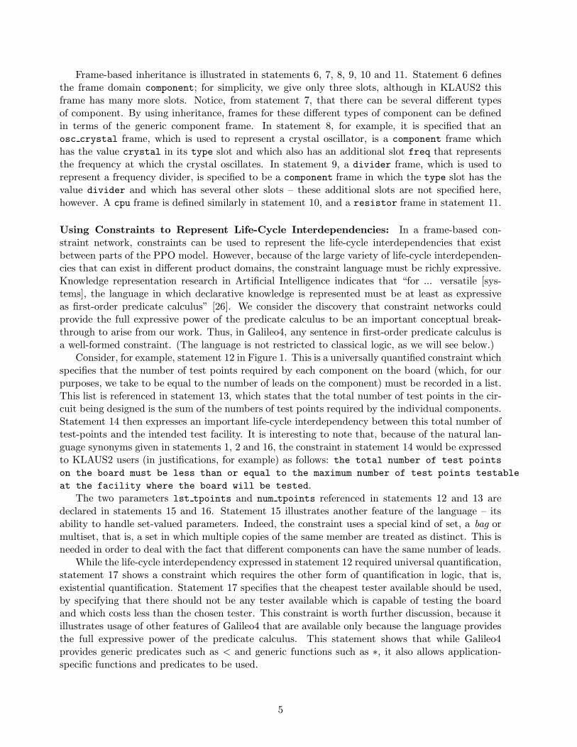
Frame-based inheritance is illustrated in statements 6, 7, 8, 9, 10 and 11. Statement 6 definesthe frame domain component; for simplicity, we give only three slots, although in KLAUS2 thisframe has many more slots. Notice, from statement 7, that there can be several different typesof component. By using inheritance, frames for these different types of component can be definedin terms of the generic component frame. In statement 8, for example, it is specified that anosc crystal frame, which is used to represent a crystal oscillator, is a component frame whichhas the value crystal in its type slot and which also has an additional slot freq that representsthe frequency at which the crystal oscillates. In statement 9, a divider frame, which is used torepresent a frequency divider, is specified to be a component frame in which the type slot has thevalue divider and which has several other slots – these additional slots are not specified here,however. A cpu frame is defined similarly in statement 10, and a resistor frame in statement 11.

Using Constraints to Represent Life-Cycle Interdependencies: In a frame-based con-straint network, constraints can be used to represent the life-cycle interdependencies that existbetween parts of the PPO model. However, because of the large variety of life-cycle interdependen-cies that can exist in different product domains, the constraint language must be richly expressive.Knowledge representation research in Artificial Intelligence indicates that “for ... versatile [sys-tems], the language in which declarative knowledge is represented must be at least as expressiveas first-order predicate calculus” [26]. We consider the discovery that constraint networks couldprovide the full expressive power of the predicate calculus to be an important conceptual break-through to arise from our work. Thus, in Galileo4, any sentence in first-order predicate calculus isa well-formed constraint. (The language is not restricted to classical logic, as we will see below.)

Consider, for example, statement 12 in Figure 1. This is a universally quantified constraint whichspecifies that the number of test points required by each component on the board (which, for ourpurposes, we take to be equal to the number of leads on the component) must be recorded in a list.This list is referenced in statement 13, which states that the total number of test points in the cir-cuit being designed is the sum of the numbers of test points required by the individual components.Statement 14 then expresses an important life-cycle interdependency between this total number oftest-points and the intended test facility. It is interesting to note that, because of the natural lan-guage synonyms given in statements 1, 2 and 16, the constraint in statement 14 would be expressedto KLAUS2 users (in justifications, for example) as follows: the total number of test points

on the board must be less than or equal to the maximum number of test points testable

at the facility where the board will be tested.The two parameters lst tpoints and num tpoints referenced in statements 12 and 13 are

declared in statements 15 and 16. Statement 15 illustrates another feature of the language – itsability to handle set-valued parameters. Indeed, the constraint uses a special kind of set, a bag ormultiset, that is, a set in which multiple copies of the same member are treated as distinct. This isneeded in order to deal with the fact that different components can have the same number of leads.

While the life-cycle interdependency expressed in statement 12 required universal quantification,statement 17 shows a constraint which requires the other form of quantification in logic, that is,existential quantification. Statement 17 specifies that the cheapest tester available should be used,by specifying that there should not be any tester available which is capable of testing the boardand which costs less than the chosen tester. This constraint is worth further discussion, because itillustrates usage of other features of Galileo4 that are available only because the language providesthe full expressive power of the predicate calculus. This statement shows that while Galileo4provides generic predicates such as < and generic functions such as ∗, it also allows application-specific functions and predicates to be used.

5

If we are to use application-specific functions and predicates, their meanings must be defined. InGalileo4, this can be done using either of the notions of extensional or intensional definition from settheory. Consider, for example, statement 18, which defines the meaning of the function cost. Themeaning of a function is a set of mappings from inputs to outputs. In statement 18, the meaningof cost is defined intensionally; the total cost of using a tester is 1.8 times the direct cost of usingthe tester, which is denoted by the function symbol price. There is a finite number of possibletesters, so the meaning of the price function is a finite set which can be defined extensionally.

Galileo4 allows extensional set definitions to be given either in the program text or in an externaldatabase file. Statement 19, for example shows that the meaning of the function price is definedby specifying that the set of pairs of values is in the database file TSTRCSTS. (We have found inour application experiments that tying function and predicate definitions to database files is a verynatural way of linking INCA systems to corporate databases.)

As with a function, the meaning of a predicate is also a set, which can also be defined either ex-tensionally or intensionally. In statement 20, we define the meaning of the predicate satisfactory

by specifying an intensional formula which uses universal quantification and two application-specificfunction symbols whose meanings are defined in statements 21 and 22.

Non-Parametric Design: In parametric design, the overall architecture of the product and itslife-cycle have already been determined and the task is merely one of establishing appropriate valuesfor the parameters of this architecture. Concurrent engineering is not this simple. Parametric designmust be accompanied by what is sometimes called componential design, in which the structure ofthe product and/or its life-cycle environment themselves are determined.

The belief is still widespread that constraint networks are incapable of addressing non-parametricdesign. However, another contribution of this research was the discovery that this limitation couldbe overcome by incorporating into constraint processing theory the notion of conditional existencefrom free logic [19]. This enables a constraint processing inference engine to deduce that, whencertain conditions are true, additional parameters must be introduced into a constraint network.This was a fundamental discovery, since it enables a constraint-based CE system to reason aboutwhen to introduce new elements into a product or life-cycle architecture. For further informationon the scientific basis for using free logic in constraint networks, see [2].

Consider, for example, statement 23. This is a universally quantified constraint which also usesthe notion of conditional existence from free logic to specify that if parameter of domain component

is used to represent a CPU, a communications controller or a digital signal processor device, thenthe parameter must have an extra slot to represent the oscillator which drives the device and musthave a further slot to represent a pullup resistor. The exists tokens in this constraint are freelogic existence specifiers, not existential quantifiers.

A more interesting usage of free logic appears in statement 24, which also uses modal logic. Theelse connective in this constraint comes from modal logic. The constraint specifies that, ideally,every crystal should oscillate at a frequency which does not exceed the maximum clock speed thatis testable by the test facility. However, it then goes on to say that if this is not possible, then anycrystal which oscillates at a faster frequency must have an ancillary divider circuit. Here, we seethe constraint network extending itself by introducing a new parameter when a certain conditionarises. This new parameter represents a new component, the necessity of whose existence has beeninferred by the system.

Optimization: Statement 17 used existential quantification to require that the cheapest possibletester be used. Since there is a finite number of possible testers, this statement illustrated opti-

6

mization of a parameter which ranged over a discrete domain. Galileo4 also supports optimizationof parameters which range over infinite domains, provided these domains are discretized into finitenumbers of equivalence sets.

Consider, for example, statement 32. This specifies that the total power consumed by the board(see statements 25 through 28) should, ideally, not exceed the goal power consumption (statement29), that it should certainly not exceed the maximum acceptable power consumption (statement30), and that between those two values the optimization tolerance is equal to a value called thepower consumption discrimination increment (statement 31).

Prioritization: By default, all constraints in a Galileo4 program are treated as being equallyimportant, and are treated as hard constraints, that is, as constraints that must be satisfied.However, we can also specify that some constraints in a program are soft. The meaning of aconstraint being soft is that the constraint should, if possible, be satisfied but, if there ever arises asituation in which violating the constraint would relieve an over-constrained situation, then it maybe ignored. We can have as many soft constraints as we want in a Galileo4 program and can assignthem different levels of hardness or priority. Constraint hardness is a number in [0,1], with 1 beingthe default and 0 being the hardness of a constraint that has been disabled completely. Statement34 is a second-order constraint which specifies that the hardness of the first-order constraint instatement 33 is 0.9.

Multiple Perspectives and Interfaces: Galileo4 enables constraint networks to be dividedinto (possibly overlapping) regions called fields of view. A field of view is that region within aconstraint network that is currently important to a user interacting with the network. A field ofview can be either global or local. The global field of view consists of the entire constraint network.A local field of view contains only a subnetwork. Each field of view contains all the parametersthat are of interest to the user, as well as all constraints which reference these parameters.

We define a field of view by specifying the set of parameters which it contains. In Figure 1,for example, we define two of the fields of view that are provided by the KLAUS2 application.Statement 35 defines a configuration field of view, which will be seen by a circuit designer, andspecifies that it contains the set of all parameters of domain component . Statement 36 definesa testability field of view and specifies that its set of parameters contains just one parameter,the test facility.

Different fields of view can be presented to their users through different styles of interface.Although the specification of these different types of interface is a simple matter in Galileo4,detailed discussion is beyond the scope of this necessarily brief presentation.

Specifications and Decisions: Galileo4 programs are interactive. A user can augment the setof constraints in the initial network that is specified in a program, by inputing additional con-straints to represent his design decisions. Thus, for example, if a test engineer decides to use anErdsys TX tester, he can indicate this decision by inputing the following equational constraint:the test facility.name = erdsys. (Note that the test engineer would not have to type thisconstraint — the desired decision can be input by using a mouse to select appropriate options ina series of pull-up menus. Furthermore, because of the system’s use of long synonyms, the engi-neer would think that he was entering the following decision: the equipment at the facility

where the board will be tested = Erdsys TX. The test engineer need never know about such“unfriendly” tokens as the test facility.name or erdsys.)

7

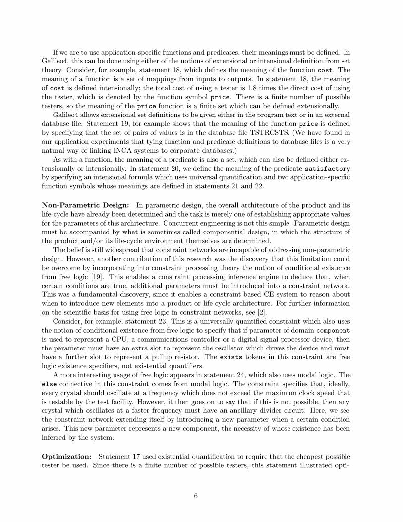
[ ]Help [ ]File [ ]New [ ]Utilities [ ]Search[ ]Up [ ]Down [ ]Focus [ ]Toggle

[ ]the equipment at the facility where the Erdsys TXboard will be tested

[ ]the maximum clock frequency testable at the 9.8facility where the board will be tested

[ ]the maximum number of test points testable 200at the facility where the board will be tested

>>>

KLAUS2 - a PWB Design Advisor (Testability)

Figure 2: The Galileo4 Scrollsheet Interface

Figure 2 shows the interface presented by KLAUS2 to the test engineer after he has selectedthe test equipment to be used for the project, and the system has inferred two of the attributes ofthis equipment via relational information represented as constraints. The largest window in thisscreen is a single-column spreadsheet, or “scrollsheet,” in which each cell occupies one or morelines. Various pull-down menus, as well as overlay windows for constraint violation detection andadvice generation, also appear when appropriate.

Decisions like the above selection of a tester are parametric design decisions. Componentialdesign decisions can be expressed by adding new parameters to the initial network that is definedby the program. Thus, for example, a circuit designer interacting with the KLAUS2 applicationcan introduce new parameters to represent various parts of his evolving circuit. To introduce aCPU, for example, he can either introduce a parameter of domain component and specify that thetype slot of this parameter has the value processor, or he can achieve exactly the same result,through frame-based inheritance, by introducing a parameter of domain cpu.

In Galileo4, we can specify which users of an application that supports multiple fields of vieware allowed to introduce new parameters and what classes of parameters they are allowed to enter.Statement 37 of Figure 1, for example, specifies that users of the configuration field of view areallowed to introduce parameters of domain component or of any domain (such as osc crystal,divider, resistor or cpu) that is a sub-class of the component domain.

One further point should be made on the representation of design decisions in Galileo4. Anysyntactically well-formed Galileo4 constraint may be used to represent a design decision. We arenot restricted to equations of the form seen above in the test engineer’s selection of test equipment.Any sentence, atomic, compound or quantified, in first-order predicate calculus, including modaland free logic as well as classical logic, can be used to represent a design agent’s decision.

Explanation: As well as specifying information by introducing new parameters and new con-straints, the user of a Galileo4 program can ask for information. He can, for example, ask for therange of allowable values for any of the parameters in a network. He can also ask for justificationsfor these ranges — whenever the range of allowable values for a parameter is reduced by a con-straint, the rationale for this reduction is noted by the run-time system as a dependency recordwhich can be accessed later for explanation purposes.

Consider, for example, a scenario in which the circuit designer specifies that he wants the crystalto oscillate at 25 MHz. Before doing so, he could have asked KLAUS2 for the range of possiblevalues. If he had done so, he would have been told that the frequency should ideally be in the range

8

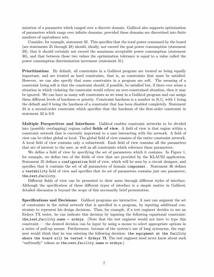
domain robot =::= datafile(qdb,$ROBOTS.DBE$).function price(robot) − > positive =::= datafile(qdb,$PRICES.DBE$).function mag capacity(robot) − > pos int =::= datafile(qdb,$MAGCPTY.DBE$).function fixtures(robot) − > pos int =::= datafile(qdb,$FIXTURES.DBE$).function throughput(robot) − > positive =::= datafile(qdb,$THRUPUT.DBE$).constant tax rate =::= 0.06.positive(reqd throughput).pos int(reqd mag capacity).pos int(reqd fixtures).robot(chosen model).positive(cost).cost = price(chosen model) * (1 + tax rate).fixtures(chosen model) >= reqd fixtures.throughput(chosen model) >= reqd throughput.mag capacity(chosen model) >= reqd mag capacity.not(exists X : fixtures(X) >= reqd fixtures and throughput(X) >= reqd throughput and

mag capacity(X) >= reqd mag capacity and price(X) < price(chosen model)).

Figure 3: A Galileo4 insertion robot selection application

[3,9.8] but that, as a last resort, any frequency in the range [3,40] could be used. If he had asked fora justification, the explanation would have referred to the fact that, in general, the only frequenciesallowed are those in the range [3,40] (see statement 4 in Figure 1) but that the test engineer’sprevious choice of an Erdsys TX tester and KLAUS2’s preference for avoiding the introduction ofancillary dividers (see the above discussion on statement 24 in the paragraph on Non-ParametricDesign) means that the preferred range is [3,9.8] because the maximum frequency testable by theErdsys TX is 9.8 MHz.

“What If” Design Reasoning: A user can always withdraw any constraint or parameter thathe has added. Thus, by introducing and withdrawing constraints and parameters, the user caninvestigate “what if” scenarios.

3 A Second Application: Insertion Robot Selection

To demonstrate the practical utility of this constraint-based approach to logic, we present in Figure3 a Galileo4 program for a type of application (manufacturing equipment selection) which is com-monly implemented using declarative rule-based programming. In this case, the application involvesselecting an insertion robot to provide required functionality at a minimum price. This practicalapplication is a short program in Galileo4 and illustrates well the advantage of constraint-basedprogramming: an equivalent declarative rule-based program would be longer and less perspicuous.

The problem of insertion robot selection is to select a robot model from among a set of availablemodels, each with varying prices, insertion magazine capacities, number of fixtures accommodated,and throughput rates. A suitable robot should have throughput, fixture, and magazine capacity atleast as great as those specified by the user of the Galileo4 program. The problem of optimal-costrobot selection is to select the suitable robot of lowest cost, factoring in the tax rate.

9

model 9520model 8581model 8582model 7001model 7002model 6001

model 9520 4499.99model 8581 3100.99model 8582 3500.99model 7001 2859.99model 7002 2959.99model 6001 1999.99

model 9520 628model 8581 128model 8582 140model 7001 88model 7002 115model 6001 60

(a) ROBOTS.DBE (b) PRICES.DBE (c) MAGCPTY.DBE

model 9520 3model 8581 6model 8582 5model 7001 6model 7002 5model 6001 1

model 9520 20model 8581 25model 8582 25model 7001 20model 7002 20model 6001 16

(d) FIXTURES.DBE (e) THRUPUT.DBE

Figure 4: Contents of Relational Database Files

All of these aspects of the problem are compactly encoded as constraints in the Galileo4 pro-gram listed in Figure 3. The first five statements in this program illustrate an advantage of ourapproach that were not exercised by the printed wiring board example, namely the natural way inwhich programs based on this approach can be linked to relational databases. Application-specificdomains, functions and predicates can be defined either extensionally or intensionally within aconstraint-based program. Alternatively, as in this program, extensional definitions can be tied tothe contents of external relational database files.

The first statement in this program declares that the extensional definition of the domain robotis the set of all robot models present in the relational file ROBOTS.DBE. Similarly, the nextfour statements declare that the extensional definitions of the four functions price, mag capacity,fixtures and throughput are in the files PRICES.DBE, MAGCPTY.DBE, FIXTURES.DBE andTHRUPUT.DBE, respectively. The sixth statement declares that tax rate 7→ 0.06.

Suppose that the contents of the files ROBOTS.DBE, PRICES.DBE, MAGCPTY.DBE, FIX-TURES.DBE and THRUPUT.DBE are as shown in Figure 4.

There are five values required of the user in order to instantiate all the parameters in theprogram: reqd throughput, reqd mag capacity, reqd fixtures, chosen model, and cost. Thesecorrespond, respectively, to the throughput (in parts per minute) that the user requires, the inser-tion magazine capacity needed, the number of fixtures required, the robot model most appropriatefor his needs and the amount he will have to spend. There are constraints in the program tospecify type restrictions for these symbols; another constraint specifies that cost is the price of thechosen model plus six percent tax; still other constraints specify that the chosen model must pro-vide the required functionality, and the final constraint specifies that there should not be anythingcheaper than the chosen model which offers this functionality.

10

3.1 Problem-Solving Versatility: An Example Scenario

To show the versatility of this program and, in a broader context, to illustrate the problem-solvingpower provided by using constraint networks the way we do, we next present an example scenariowhich samples the wide variety of problems that the program can be used to solve.

Even this simple a program can be used to solve a wide variety of problems. The user is freeto invoke forward-chaining by asserting (and later retracting) additional arbitrary constraints, theonly restriction being that each such sentence must reference at least one parameter from the set{reqd throughput, reqd mag capacity, reqd fixtures, cost, chosen model}. Alternatively, the usercan invoke backward-chaining by asking the system to determine the value of any of the parametersin this set. The following example scenario illustrates some of this versatility.

Suppose there is a manufacturing operation, with a limited budget, which hopes to buy a robotwhich will satisfy two needs: a lot of magazine capacity and sufficient fixtures.

Immediately after invoking this program, the user specifies what he estimates to be the amountof magazine capacity needed, by interactively asserting reqd mag capacity = 200. The systemreports that chosen model 7→ model 9520 and that cost 7→ 4769.9894. If the user asks for ajustification, the system will explain that these conclusions were caused by the requirements that

mag capacity(chosen model) >= reqd mag capacity

and thatcost = price(chosen model) ∗ (1 + tax rate).

But suppose that this is more than management wants to spend. The user retracts reqd mag capacity= 200 and asserts cost =< 4000. If the user asks to be shown the current set of possible valuesfor reqd mag capacity, he will be told that it is any positive integer up to 140, which is the maga-zine capacity of the model 8582, the robot with the largest magazine capacity whose cost does notexceed 4000.

Suppose that the user now decides to stop volunteering information and tells the system todetermine the appropriate robot, asking whatever questions it sees fit along the way. Then, triggeredby the specification fixtures(chosen model) >= reqd fixtures, the system asks the user to specifya value for reqd fixtures and, in response, suppose the user asserts that reqd fixtures = 6. Thesystem then asks for the reqd throughput; the user has no specific speed in mind but, choosinga ball-park minimum, he asserts that reqd throughput >= 18. The system then asks for thereqd mag capacity; the user, remembering the previous information about the set of possible valuesfor this parameter, responds by asserting that reqd mag capacity = 140.

However, this causes a contradiction, because the maximum magazine capacity offered by anyrobot which can support six fixtures is 128. The system suggests that the user should retract oneof the two assertions, reqd fixtures = 6 or reqd mag capacity = 140.

However, suppose the user wants to know why he cannot have the model 8582. Therefore,before adopting any of the above suggestions, he asserts chosen model = model 8582. In response,he is told that this contradicts the requirements that fixtures(chosen model) >= reqd fixturesand reqd fixtures = 6.

Recognizing that he cannot get a robot which satisfies all his needs, the user decides that, fornow, he will just buy a robot with a smaller insertion magazine. So, he retracts chosen model =model 8582 and reqd mag capacity = 140, and asserts that reqd mag capacity = 10.

The set of possible values for chosen model which is allowed by the user’s stated functionalityrequirements contains two robots, the model 8581 and the model 7001. The system cannot decidefor certain, however, that either of these robots is suitable, because the user has not been specificenough about reqd throughput.

11

Suppose, however, that the user now chooses a ball-park maximum for reqd throughput andasserts that reqd throughput < 19. Both of the robots just mentioned provide the required func-tionality but, because of the constraint

not(exists X : fixtures(X) >= reqd fixtures and throughput(X) >= reqd throughput andmag capacity(X) >= reqd mag capacity and price(X) < price(chosen model)).

the system can choose the cheaper of the two robots, reporting that chosen model 7→ model 7001.

4 Comparative Discussion

Although it is less widely used than rule-based programming, constraint-based programming is nota new idea: the first constraint-based programming system was developed almost 30 years ago [29].The major factor inhibiting a widespread application of constraint-based programming has beenthe highly specialized nature of the constraint-based programming systems available. For example,the first constraint-based system, Sketchpad [29] was oriented towards graphics while Thinglab[6] was developed for simulation applications. An early language which offered more generalitywas Constraints [28] but several important notions, including inequality, were not available in thelanguage. Magritte [14] was restricted to algebraic relationships and did not support the use ofarbitrary application-specific predicates, functions and domains.

More recently, there has been a surge of interest in the relationship between constraints and logicprogramming. Several languages based on Prolog have been developed, most notably CLP(<) [17];Prolog III [8]; and CHIP [11]. In these languages, which are generically known as the CLP languages,unification in the Herbrand universe is supplemented with constraint processing of linear equationsor inequalities over the numbers. CHIP also uses arc-consistency to process atomic constraintsinvolving application-specific predicates defined over finite domains.

Galileo4 provides richer expressive power than any other constraint-based programming lan-guage because it allows the theory Γ used to specify a constraint network to contain arbitraryFOPC sentences (atomic, compound or quantified) about a many-sorted universe of discourse whichincludes, besides the real numbers <, any arbitrary application-specific sorts. Nearly all other con-straint languages restrict the theory to ground sentences. For example, in the CLP languages, thetheory used to specify a constraint network is the set of conjuncts in a compound goal presentedto the top-level interpreter; although logic variables may appear in such a goal, these are implicitlysubject to existential quantification, which means that, essentially, they are uninterpreted constantsymbols, making the constraints ground sentences. One language which does seem to supportquantified constraints is CONSUL [7], but it restricts the universe of discourse to the integers.

Expressiveness in knowledge representation, however, is only one side of the coin. Constraint-based languages also differ in the inferential competence and efficiency offered by their run-timesystems. One of the earliest, and most commonly used, constraint propagation mechanisms is localpropagation of known states, which is efficient but incomplete. The simplex-like algorithm used inthe CLP languages is more complete (that is, can draw more inferences given the same premises)than local propagation of known states and considerable effort has been devoted to developingefficient and fast implementations. Until recently, there was little cross-fertilization between theliterature on finite domain CSPs and that on constraint-based programming languages. The firstattempt to amalgamate ideas from these two bodies of work seems to have been the CLP languageCHIP [11], in which the application of simplex to constraints on the rationals was supplementedby the application of arc consistency to constraints on application-specific finite domains.

The CCP algorithm used in Galileo4 takes the idea of borrowing concepts from the finite domainCSP literature a step further, by integrating local propagation of known states with versions of

12

arc and path consistency that have been generalized to constraints of arbitrary arity on infinitedomains. The inferential competence of the resulting algorithm is better in some respects, butworse in others, than the algorithms used in the CLP languages. For example, there are severalclasses of problem involving sets of simultaneous non-linear equations that can be handled byCCP [27], while the CLP languages can only handle non-linear constraints if they become linearduring the propagation process. However, the CCP algorithm is limited to handling systems ofsimultaneous equations in which each equation involves only two unknowns or is reduced to abinary equation during propagation. Although there has been considerable research into constraintpropagation algorithms for finite domain networks, and despite the fact that constraint processinghas been around a long time, constraint propagation for infinite domain networks is still a relativelyundeveloped field. We view CCP as being capable of further improvement; for example, an obvioustopic to investigate is the amalgamation of simplex analysis with the battery of techniques currentlyused in CCP.

The query interface to CLP languages is basically the same as that provided by the earlyPrologs. That this interface is inadequate for constraint processing was recognized in [22] where anew interface was proposed. It is interesting to note that the “answer manipulation commands”which they propose would allow the same kind of non-monotonic editing of goals as the Galileo4user can achieve by asserting/retracting assumptions.

5 The Relationship Between Constraint Networks and ConstraintLogic

This chapter presents an attempt to make the full FOPC available in an INCA-construction lan-guage known as Galileo4. In the run-time system for this language, inference is based on a treat-ment of semantic entailment as constraint propagation. Very simply, constraint propagation is thecommunication of parameter values through the network to all constraints which refer to thoseparameters. This propagation process occurs omnidirectionally each time a parameter acquireseither a new or revised value or a restriction of its domain of possible values. These new valuesmay in turn stimulate further inference, and the process iterates until quiescence. To provide thetheoretical basis for this approach, we review model theory and constraint processing and then weshow how the satisfiability of a set of sentences in logic can be viewed as the consistency of a setof constraints in a constraint network.

5.1 A Review of Model Theory

The truth of a sentence in logic is based on the interpretation of the symbols in the sentence.Consider some first-order logic language L = 〈P,F ,K〉, where P is the vocabulary of predicatesymbols, F is the vocabulary of function symbols, and K is the vocabulary of constant symbols. Atheory Γ in L is satisfiable iff there exists some model M = 〈U ,I〉 of the language L under whichevery sentence in Γ is true, that is, iff there exists some M such that M |= Γ.1

In a model M = 〈U ,I〉 for the language L = 〈P,F ,K〉, U is a universe of discourse while I isan interpretation function for the constant, predicate, and function symbols of L. For every κ ∈ K,I(κ) is an element of U . For every n-ary predicate symbol p ∈ P, I(p) is an n-ary relation over U .For every n-ary function symbol f ∈ F , I(f) is an (n + 1)-ary relation over U . For a functionalexpression f(a1, ..., an), where f is an n-ary function symbol and the terms ai, i = 1..n, are either

1The notationM |= Γ means that any interpretation of the symbols inM satisfyingM will simultaneously satisfyΓ.

13

constant symbols or nested functional expressions, I(f(a1, ..., an)) is an element of U such thatI(f) contains the (n+ 1)-ary tuple 〈I(a1), ...,I(an),I(f(a1, ..., an))〉.

Let M |= γ, where γ is a sentence, mean that γ is true under the model M and let M{X 7→u}mean a model containing the extended interpretation function I ∪ {X 7→ u}.2 The rules fordetermining whether a sentence is true under a model are as follows:

• M |= p(a1, ..., an) iff 〈I(a1), ...,I(an)〉 is in I(p).

• M |= ¬A iff M 6|= A.

• M |= A ∧B iff M |= A and M |= B.

• M |= A ∨B iff M |= A or M |= B.

• M |= A⇒ B iff M 6|= A or M |= B.

• M |= A⇔ B iff (M 6|= A and M 6|= B) or (M |= A and M |= B).

• M |= (∀X)A iff M{X 7→u} |= A for every u ∈ U .

• M |= (∃X)A iff M{X 7→u} |= A for some u ∈ U .

5.2 A Review of Constraint Processing

A constraint specifies some relationship that must be satisfied by the values, chosen from somedomain, which are assumed by a group of parameters. A constraint network is a collection ofconstraints which are interlinked by virtue of having some parameters in common.

There has developed a considerable body of literature on the processing of constraint networks.This literature tends to fall into two broad classes. In the first kind of paper, which is where theterm CSP is used, constraint networks are assumed to have finite domains [10, 13, 16, 21, 23, 25], therelationships imposed by constraints are expressed extensionally, and the CSPs are NP-complete.Although the CSPs in this literature can be solved by backtracking search, the exponential com-putational cost of such search algorithms has led to the development of preprocessing algorithms[12, 15, 21, 24], called consistency algorithms, which aim to reduce thrashing, that is, repeatedly ex-ploring parameter assignments that cannot result in a solution, by a priori elimination of parameterto value mappings that cannot belong to any consistent valuation of the network parameters.

In the second class of literature on constraint processing, constraint networks are allowed, butnot required, to have infinite domains, and the restrictions imposed by constraints can be expressedintensionally. In this literature, which includes that dealing with Constraint Logic Programming(CLP) [8, 11, 17], the problem-solving techniques include local propagation of known states [20] anda simplex-like version of gaussian elimination [17]. Consider, for example, the CLP(<) language,which is based on Prolog and in which constraint parameters can range over the real numbers <.In this language, a constraint network is treated as a conjunctive goal which is submitted to thetop-level of a Prolog-like interpreter; for example, a goal such as

?- Load = Area * Stress, Load = 30, Area = 5.

is a network containing three constraints which intensionally specify restrictions on the values thatcan be assumed by the three parameters, Load, Area and Stress. When the CLP(<) interpreterresponds with

2The notation X 7→ u indicates that symbol X is assigned the semantic interpretation u.

14

Load = 30 Area = 5 Stress = 6 ***Yes

it is giving an existence proof that there is a valuation for the parameters which satisfies all theconstraints in the network.

In this second body of work, although constraint networks may have infinite domains, severelimits have been placed on the use of intensional specifications. Systems have restricted the typesof logic connective that can be used and the situations in which they can be used. Furthermore,in most systems, only ground sentences may be used. In CLP(<), for example, the free variablesin a goal are treated as being implicitly subject to existential quantification, which means thateffectively they are equivalent to uninterpreted constant symbols. Thus, the goal shown above canbe regarded as a conjunction of three ground sentences, load = area ∗ stress, load = 30, and area= 5, in which there are three uninterpreted constant symbols, load, area, and stress. The task ofthe interpreter is then to determine whether there is an interpretation for these constant symbolswhich satisfies all three ground sentences. Constraints in CLP(<) cannot use quantification; it isnot possible, for example, to submit goals such as

?- Load = Area * Stress, Load = 30,Area = 5, (all X : Area < X < Stress implies X > Load/2).

in which the last constraint is a universally quantified sentence. In the one language known toallow explicit quantification [7], the domain is restricted to the integers and it is unclear whetherquantifiers may be arbitrarily nested.

Our work is directed towards removing these limitations and allowing arbitrary FOPC formulaeto be used as constraints.

5.3 Definitions

The literature contains several definitions of constraint satisfaction, with varying degrees of formal-ity. One consequence of the lack of formal definition of the concept is that many authors fail todistinguish between notions of decision, exemplification, and enumeration. In an effort to removethis ambiguity and to set the scene for a mapping between constraint processing and semanticmodeling, we propose the following definitions.

Definition, Constraint Network:A constraint network is a triple 〈U ,X,C〉 where U is a universe of discourse, X is a finite tuple ofq non-recurring parameters, and C is a finite set of of r constraints. Each constraint Ck(Tk) ∈ Cimposes a restriction on the allowable values for the ak parameters in Tk, a sub-tuple of X, byspecifying that some subset of the ak-ary Cartesian product Uak contains all acceptablecombinations of values for these parameters.

The overall network constitutes an intensional specification of a joint possibility distribution forthe values of the parameters in the network. This joint possibility distribution, called the networkintent [2], is a q-ary relation on Uq, as defined below.

Definition, Projection:Let R be a q-ary relation with indices 〈x1, x2, ..., xq〉, and let T = 〈t1, t2, ..., tm〉 be an m-arysubtuple of 〈x1, x2, ..., xq〉. The projection of R onto T , denoted proj(R,T ), is the largest set ofm-tuples 〈bt1 , bt2 , ..., btm〉 such that there is some q-tuple 〈cx1 , cx2 , ..., cxq 〉 in R for which btj = ctj ,for all j = 1, 2, ...,m.

15

Definition, Cylindrical Extension:Let X = 〈x1, x2, ..., xq〉 be a q-ary tuple of indices defining a Cartesian space Uq, let T =〈t1, t2, ..., tm〉 be a subtuple of 〈x1, x2, ..., xq〉, and let C(T ) be a relation on the space defined byT . The cylindrical extension of C(T ) into the space defined by X, denoted E(X), is the largestrelation R on that space such that proj(R,T ) = C(T ).

Definition, The Intent of a Constraint Network:The intent of a constraint network 〈U ,X,C〉 is

ΠU ,X,C = E1(X) ∩ ... ∩Er(X),where, for each constraint Ck(Tk) ∈ C, Ek(X) is its cylindrical extension into the Cartesian spacedefined by X.

The network intent is a set of q-tuples, each tuple giving, for the q parameters in X, a valuationwhich is acceptable to all the constraints in C.

A constraint network is consistent if the network intent is not the empty set. Three forms ofconstraint satisfaction problem (CSP) can be distinguished:

Definition, The Decision CSP:Given a network 〈U ,X,C〉, decide whether ΠU ,X,C is non-empty.

Definition, The Exemplification CSP:Given a network 〈U ,X,C〉, return some tuple from ΠU ,X,C, if ΠU ,X,C is non-empty, or return nilotherwise.

Definition, The Enumeration CSP:Given a network 〈U ,X,C〉, return ΠU ,X,C.

5.4 Networks and Models

A total interpretation function for a first-order language L is a set of mappings, such that everypredicate and function symbol of L is mapped onto a relation of the appropriate arity over someuniverse of discourse U , and such that every constant symbol of L is mapped onto a member of U .A partial interpretation function for L is a set of mappings which does not contain a mapping forevery symbol of L; at least one constant, predicate, or function symbol is not given a mapping.

Consider the class of problem in which, given a theory Γ written in a first-order languageL = 〈P,F ,K〉 and a partial interpretation function Ip for L in terms of a universe U , one has todetermine whether there is any total interpretation I for L such that Ip ⊂ I and 〈U ,I〉 |= Γ. This,the class of modeling problems, can be divided into several subclasses.

Class 1 modeling problems are those where Ip contains interpretations for all the predicateand function symbols of L, where a finite subset of the constant symbols are uninterpreted, whereevery sentence in Γ references at least one of the uninterpreted constant symbols, and where eachuninterpreted constant symbol is referenced by at least one sentence in Γ. Although there areseveral other classes, (for example, those modeling problems where some subset of the function andpredicate symbols lack interpretations), Class 1 problems are those that are of interest here.

Class 1 problems can be further subdivided, as follows:

Definition, The Class 1 Decision Modeling Problem:Given L = 〈P,F ,K′ ∪ K′′〉, U , Ip and Γ, where Ip interprets, in terms of U , all and only thesymbols in P ∪ F ∪K′, K′′ is finite, each sentence in Γ references at least one symbol in K′′, andeach symbol in K′′ is referenced by at least one sentence γ ∈ Γ, decide whether there exists any Jsuch that J interprets all symbols in K′′ and 〈U ,Ip ∪ J 〉 |= Γ.

16

Definition, The Class 1 Exemplification Modeling Problem:Given L = 〈P,F ,K′ ∪ K′′〉, U , Ip and Γ, as in the Class 1 Decision Modeling problem, return, ifone exists, some J such that J interprets all symbols in K′′ and 〈U ,Ip ∪ J 〉 |= Γ; if no such Jexists, return nil.

Definition, The Class 1 Enumeration Modeling Problem:Given L = 〈P,F ,K′ ∪ K′′〉, U , Ip and Γ, as in the Class 1 Decision Modeling problem, return theset of all J such that J interprets all symbols in K′′ and 〈U ,Ip ∪ J 〉 |= Γ.

These three forms of modeling problem can be shown to correspond to the three forms of CSPdefined in Section 5.3. In what follows, let ~AB, where A and B are tuples of the same arity, bethe mapping function from the components of A onto those of B in which each component of thetuple A is mapped onto the component in the corresponding position of tuple B; for example, if A= 〈x, y〉 and B = 〈4, 2〉, then ~AB = { x 7→ 4, y 7→ 2 }.

Theorem 1Given L = 〈P,F ,K′ ∪ K′′〉, U , Ip and Γ, where Ip interprets, in terms of U , all and only thesymbols in P ∪ F ∪K′, K′′ is finite, each sentence in Γ references at least one symbol in K′′, andeach symbol in K′′ is referenced by at least one sentence γ ∈ Γ. Let 〈U ,X,C〉 be a constraintnetwork such that X is the lexical ordering of the elements of K′′ and such that |C| = |Γ|, witheach sentence γ ∈ Γ having a corresponding constraint C(T ) ∈ C such that T is the lexicalordering of those elements of K′′ which appear in γ and 〈U ,Ip ∪ ~T t〉 |= γ for all tuples t ∈ C(T ).

Then 〈U ,Ip ∪ ~Xτ〉 |= Γ for all tuples τ ∈ ΠU ,X,C.

The proof of this theorem appears in the appendix.Thus, the set of all ~Xτ where τ ∈ ΠU ,X,C is the set of all J such that J interprets all symbols

in K′′ and 〈U ,Ip ∪ J 〉 |= Γ. Thus, the Class 1 Decision Modeling Problem corresponds to theDecision CSP, the Class 1 Exemplification Modeling Problem corresponds to the ExemplificationCSP and the Class 1 Enumeration Modeling Problem corresponds to the Enumeration CSP.

5.4.1 Example 1

Consider a language L, a universe of discourse U , and a partial interpretation Ip for L in terms ofU , as follows:

Language: L = 〈{s, t}, ∅, {a, b, c}〉Universe of discourse: U = {1,2,3,4,5,6,7}Partial Interpretation:

Ip = { s 7→ {5,7},t 7→ {〈1, 4〉, 〈2, 5〉, 〈3, 6〉, 〈4, 7〉, 〈5, 1〉, 〈5, 3〉,

〈6, 2〉, 〈6, 3〉, 〈6, 7〉, 〈7, 1〉, 〈7, 3〉},b 7→ 7 }.

Suppose that, given the above situation, we need to determine the satisfiability of the followingtheory:

Γ = {t(a, c), (∀X)(s(X)⇒ t(X,a)), t(c, b)}.

The constraint network 〈U ,X,C〉 corresponding to this is a possibility distribution, such thatΓ is satisfied, for interpretations of the remaining uninterpreted constant symbols of L, in this casefor a and c. The components of the network are:

17

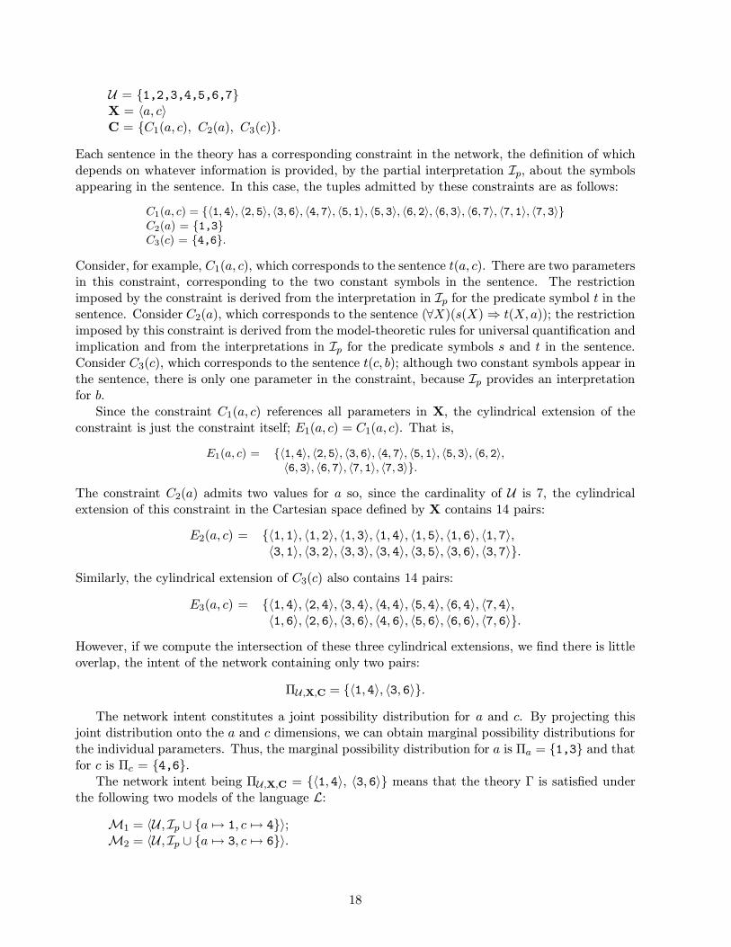
U = {1,2,3,4,5,6,7}X = 〈a, c〉C = {C1(a, c), C2(a), C3(c)}.

Each sentence in the theory has a corresponding constraint in the network, the definition of whichdepends on whatever information is provided, by the partial interpretation Ip, about the symbolsappearing in the sentence. In this case, the tuples admitted by these constraints are as follows:

C1(a, c) = {〈1, 4〉, 〈2, 5〉, 〈3, 6〉, 〈4, 7〉, 〈5, 1〉, 〈5, 3〉, 〈6, 2〉, 〈6, 3〉, 〈6, 7〉, 〈7, 1〉, 〈7, 3〉}C2(a) = {1,3}C3(c) = {4,6}.

Consider, for example, C1(a, c), which corresponds to the sentence t(a, c). There are two parametersin this constraint, corresponding to the two constant symbols in the sentence. The restrictionimposed by the constraint is derived from the interpretation in Ip for the predicate symbol t in thesentence. Consider C2(a), which corresponds to the sentence (∀X)(s(X)⇒ t(X,a)); the restrictionimposed by this constraint is derived from the model-theoretic rules for universal quantification andimplication and from the interpretations in Ip for the predicate symbols s and t in the sentence.Consider C3(c), which corresponds to the sentence t(c, b); although two constant symbols appear inthe sentence, there is only one parameter in the constraint, because Ip provides an interpretationfor b.

Since the constraint C1(a, c) references all parameters in X, the cylindrical extension of theconstraint is just the constraint itself; E1(a, c) = C1(a, c). That is,

E1(a, c) = {〈1, 4〉, 〈2, 5〉, 〈3, 6〉, 〈4, 7〉, 〈5, 1〉, 〈5, 3〉, 〈6, 2〉,〈6, 3〉, 〈6, 7〉, 〈7, 1〉, 〈7, 3〉}.

The constraint C2(a) admits two values for a so, since the cardinality of U is 7, the cylindricalextension of this constraint in the Cartesian space defined by X contains 14 pairs:

E2(a, c) = {〈1, 1〉, 〈1, 2〉, 〈1, 3〉, 〈1, 4〉, 〈1, 5〉, 〈1, 6〉, 〈1, 7〉,〈3, 1〉, 〈3, 2〉, 〈3, 3〉, 〈3, 4〉, 〈3, 5〉, 〈3, 6〉, 〈3, 7〉}.

Similarly, the cylindrical extension of C3(c) also contains 14 pairs:

E3(a, c) = {〈1, 4〉, 〈2, 4〉, 〈3, 4〉, 〈4, 4〉, 〈5, 4〉, 〈6, 4〉, 〈7, 4〉,〈1, 6〉, 〈2, 6〉, 〈3, 6〉, 〈4, 6〉, 〈5, 6〉, 〈6, 6〉, 〈7, 6〉}.

However, if we compute the intersection of these three cylindrical extensions, we find there is littleoverlap, the intent of the network containing only two pairs:

ΠU ,X,C = {〈1, 4〉, 〈3, 6〉}.

The network intent constitutes a joint possibility distribution for a and c. By projecting thisjoint distribution onto the a and c dimensions, we can obtain marginal possibility distributions forthe individual parameters. Thus, the marginal possibility distribution for a is Πa = {1,3} and thatfor c is Πc = {4,6}.

The network intent being ΠU ,X,C = {〈1, 4〉, 〈3, 6〉} means that the theory Γ is satisfied underthe following two models of the language L:

M1 = 〈U ,Ip ∪ {a 7→ 1, c 7→ 4}〉;M2 = 〈U ,Ip ∪ {a 7→ 3, c 7→ 6}〉.

18

Augmenting a theory by asserting an additional sentence often reduces the number of possiblemodels. Suppose we augment Γ by adding the assertion t(b, c) to the theory. From Ip(t) and Ip(b),the corresponding constraint is C4(c) = {1, 3}. Since this constraint admits neither of the twovalues for c that are allowed by the existing network, the new network intent will be the emptyset. Thus, there is no model 〈U ,I〉,Ip ⊂ I, of the language L under which the following theory issatisfied:

Γ′ = {t(a, c), (∀X)(s(X)⇒ t(X,a)), t(c, b), t(b, c)}.

Suppose, however, we retract t(b, c) and assert t(c, a). The resultant theory in this case,

Γ′′ = {t(a, c), (∀X)(s(X)⇒ t(X,a)), t(c, b), t(c, a)}

is satisfiable. However, the new network intent would be a strict subset of ΠU ,X,C, namelyΠU ,X,C′′ = {〈3, 6〉}. The fact that ΠU ,X,C′′ admits only one pair means that unique values 3

and 6 can be inferred for a and c, respectively.

5.4.2 Example 2

In Example 1, the universe of discourse was finite and the predicate symbols had finite interpre-tations. The following example has an infinite universe and some of the predicate and functionsymbols have infinite sets as their interpretations:

Language: L = 〈{positive, nonnegative,=,≤, h, j, k, g},{∗, l,m},R∪ {a, b, c, d, e, f, g1, g2, g3, g4}〉

Universe of discourse: U = < ∪ {g1, g2, g3, g4}Partial Interpretation:

Ip = IR ∪{ positive 7→ <+

nonnegative 7→ <0+

= 7→ {〈X,Y 〉|X ∈ U ∧ Y ∈ U∧equals(X,Y )}≤ 7→ {〈X,Y 〉|X ∈ < ∧ Y ∈ <∧leq(X,Y )}h 7→ {X |X ∈ <+∧ leq(X, 10)}j 7→ <+

k 7→ <−g 7→ {g1,g2,g3,g4}∗ 7→ {〈X,Y, Z〉|X ∈ < ∧ Y ∈ < ∧ Z ∈ <∧equals(Z,times(X,Y ))}l 7→ {〈g1, 200〉, 〈g2, 250〉, 〈g3, 350〉, 〈g4, 390〉}m 7→ {〈g1, 230〉, 〈g2, 190〉, 〈g3, 240〉, 〈g4, 245〉}g1 7→ g1

g2 7→ g2

g3 7→ g3

g4 7→ g4 }.Theory: Γ = {positive(a), h(b), positive(c), g(e), d = a ∗ f, j(f)⇒ f ≤ l(e), k(f)⇒ f ≤ m(e),

(∀X)(g(X)⇒ m(X) ≤ l(e)), (∃X)(l(X) > l(e)), a = b ∗ c}.

In the language L, R is the set of constant symbols composed from the characters +,−, . and0..9 according to a grammar for real numeric strings. R is distinguished from <, the set of realnumbers. In this chapter, to distinguish between symbols of L and entities of U , we use typewriterfont for the latter. Thus, 200 ∈ R and g1 are constant symbols, while 200 ∈ < and g1 are in theuniverse of discourse. In the partial interpretation Ip, IR is a bijection from the constant symbolsin R onto Qf , the set of finite-length rational numbers, Qf ⊂ Q ⊂ <; thus IR contains mappingssuch as 200 7→ 200.

19

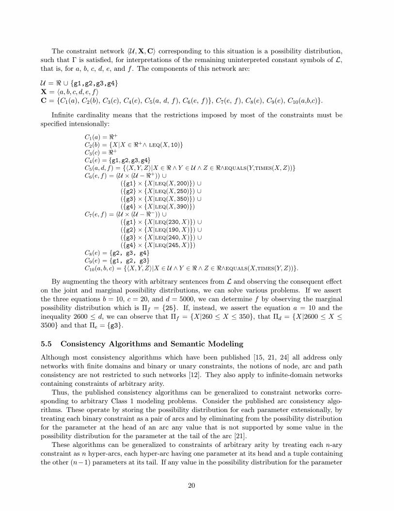
The constraint network 〈U ,X,C〉 corresponding to this situation is a possibility distribution,such that Γ is satisfied, for interpretations of the remaining uninterpreted constant symbols of L,that is, for a, b, c, d, e, and f . The components of this network are:

U = < ∪ {g1,g2,g3,g4}X = 〈a, b, c, d, e, f 〉C = {C1(a), C2(b), C3(c), C4(e), C5(a, d, f), C6(e, f)}, C7(e, f), C8(e), C9(e), C10(a,b,c)}.

Infinite cardinality means that the restrictions imposed by most of the constraints must bespecified intensionally:

C1(a) = <+

C2(b) = {X |X ∈ <+∧ leq(X, 10)}C3(c) = <+

C4(e) = {g1, g2, g3, g4}C5(a, d, f) = {〈X,Y, Z〉|X ∈ < ∧ Y ∈ U ∧ Z ∈ <∧equals(Y,times(X,Z))}C6(e, f) = (U × (U − <+)) ∪

({g1} × {X |leq(X, 200)}) ∪({g2} × {X |leq(X, 250)}) ∪({g3} × {X |leq(X, 350)}) ∪({g4} × {X |leq(X, 390)})

C7(e, f) = (U × (U − <−)) ∪({g1} × {X |leq(230, X)}) ∪({g2} × {X |leq(190, X)}) ∪({g3} × {X |leq(240, X)}) ∪({g4} × {X |leq(245, X)})

C8(e) = {g2, g3, g4}C9(e) = {g1, g2, g3}C10(a, b, c) = {〈X,Y, Z〉|X ∈ U ∧ Y ∈ < ∧ Z ∈ <∧equals(X,times(Y, Z))}.

By augmenting the theory with arbitrary sentences from L and observing the consequent effecton the joint and marginal possibility distributions, we can solve various problems. If we assertthe three equations b = 10, c = 20, and d = 5000, we can determine f by observing the marginalpossibility distribution which is Πf = {25}. If, instead, we assert the equation a = 10 and theinequality 2600 ≤ d, we can observe that Πf = {X|260 ≤ X ≤ 350}, that Πd = {X|2600 ≤ X ≤3500} and that Πe = {g3}.

5.5 Consistency Algorithms and Semantic Modeling

Although most consistency algorithms which have been published [15, 21, 24] all address onlynetworks with finite domains and binary or unary constraints, the notions of node, arc and pathconsistency are not restricted to such networks [12]. They also apply to infinite-domain networkscontaining constraints of arbitrary arity.

Thus, the published consistency algorithms can be generalized to constraint networks corre-sponding to arbitrary Class 1 modeling problems. Consider the published arc consistency algo-rithms. These operate by storing the possibility distribution for each parameter extensionally, bytreating each binary constraint as a pair of arcs and by eliminating from the possibility distributionfor the parameter at the head of an arc any value that is not supported by some value in thepossibility distribution for the parameter at the tail of the arc [21].

These algorithms can be generalized to constraints of arbitrary arity by treating each n-aryconstraint as n hyper-arcs, each hyper-arc having one parameter at its head and a tuple containingthe other (n−1) parameters at its tail. If any value in the possibility distribution for the parameter

20

at the head of a hyper-arc is not supported by some (n − 1)-tuple of values for the other (n − 1)parameters at the tail of the hyper-arc, the value can be removed from the possibility distribution.

Algorithms for arc consistency can be generalized to infinite domains by storing infinite pos-sibility distributions intensionally. Removing unsupported values from the intensionally-definedpossibility distribution for a parameter can be done by making the intensional formula suitablymore specific. Whenever it is recognized that the possibility distribution has been restricted to afinite set of suitably small cardinality, the representation can be converted to an extensional format,if necessary.

The published path consistency algorithms can be generalized in a similar fashion. Thesealgorithms operate by storing extensionally the joint possibility distribution corresponding to aconstraint and by eliminating from the extension any tuple that is not supported by all other pathsbetween the parameters in the constraint. The algorithms can be generalized to the infinite setsof tuples that are admitted by constraints in infinite-domain networks, by storing infinite jointpossibility distributions intensionally. Removing unsupported tuples from an intensionally-definedjoint possibility distribution can be done by making the intensional formula suitably more specific.

Thus, treating Class 1 modeling problems as CSPs of the generalized types defined in Sec-tion 5.3, and generalizing the published consistency algorithms appropriately, would appear to bean attractive computational companion to a representation employing the full FOPC. There isa problem, however, in that generalizing the consistency algorithms in this way means that theintensional formulae may become arbitrarily complex, which raises the specter of undecidability.3

Even the satisfiability of formulae that are theoretically decidable may be beyond the competenceof whatever inference algorithm we embed in our system.

The way to escape from this problem is to side-step it. No inference algorithm for the fullFOPC can be sound, terminating and complete. Soundness is a sine qua non4 and, to be practical,an algorithm has to terminate. However, if we take the right attitude to possibility distributions,incompleteness need not be a disaster. This suggests, therefore, a framework for a research effortdirected at supporting the full FOPC as a programming language for knowledge-based applications.Applications are cast as Class 1 modeling problems, with salient parameters being treated asconstant symbols in an FOPC theory which represents the currently available knowledge about theapplication area. Users of an application program interact with the program by augmenting thetheory embedded in the program with assertions about their particular problem instance and byinterpreting the computed marginal possibility distributions appropriately. The results of researchleading to improved inferential competence can be incorporated into the run-time system for thelanguage over time without altering application programs, in a fashion analogous to the way in whichimprovements to the run-time speed of a language interpreter have no impact on the correctnessof programs in the language.

6 Galileo4 Revisited

As we have seen, Galileo4 is a programming language highly applicable to supporting production.On a more formal plane, Galileo4 is firmed rooted in the notion of constraint networks and onthe relationship, discussed above, between such networks and possibility distributions for semantic

3A problem is said to be undecidable if it is not possible even in theory to devise an algorithm for solving it. A classof problems is undecidable if it contains at least one specific problem instance which is undecidable. For example,while many specific satisfiability problems in FOPC have algorithmic solutions, not all do, and so satisfiability inFOPC is undecidable.

4Unless unsound inferences are allowed in a principled way, by the introduction of non-monotonic common-senseassumptions.

21

models of theories written in the full FOPC. The run-time system for the language is a test-bed for various approaches to computing the intent of sets of well-formed FOPC formulae and togeneralizing the consistency algorithms.

6.1 Galileo4 Programs

An application program in Galileo4 provides a declarative specification of a constraint network,analogous to the problem specifications in Example 1 and Example 2. That is, in general, anapplication program in Galileo4 specifies a first-order language L = 〈P,F ,K〉, a theory Γ containingclosed sentences from that language, a universe of discourse U , and a partial interpretation functionIp for L. Of these, only the theory Γ must always be specified explicitly, because, in many situations,a default universe and a default partial interpretation provided by the run-time system are adequate,while the system can determine the language L by computing the union of the constant symbols usedin Γ with the vocabulary of constant symbols in the default language Lg = 〈Pg,Fg,Kg〉 providedby the run-time system. In Lg, Kg = R contains the real numeric strings, Pg contains names ofstandard predicates (=, =<, etc.), and Fg contains names of standard functions (∗,+, etc.). Therun-time system also provides a default universe of discourse Ug = < and an interpretation functionIg for Lg giving the standard interpretations in terms of Ug. For example, the constant symbols inKg are mapped onto the intended finite-length rational numbers with interpretations such as 1 7→ 1

and 2.1 7→ 2.1.The language L = 〈P,F ,K〉 defined by an application program in Galileo4 has the following

components: P = Pg ∪ {predicate symbols defined in the program}; F = Fg ∪ {function symbolsdefined in the program}; K = Kg ∪ {constant symbols used in the program}. The universe ofdiscourse U defined by a Galileo4 program is the union of Ug = < with any application-specificdomains that are defined in the program. The partial interpretation function Ip defined by theprogram is the union of the set of mappings in Ig with any application-specific interpretations thatare provided in the program.

6.2 The Galileo4 Run-Time System

The Galileo4 run-time system attempts to compute the marginal possibility distribution Πx, theprojection of ΠU ,X,C on the dimension x, for each parameter x in X in the network 〈U ,X,C〉 thatis defined by a Galileo4 program. In general, it is only possible to compute Π̃x, an approximationto Πx such that Πx ⊆ Π̃x. However, in many networks the run-time system can compute Πx for allx in X.

6.2.1 Propagation Algorithm

An important aspect of our ongoing research consists of the development of constraint propagationalgorithms which compute better approximations to the marginal possibility distributions for pa-rameters in infinite domain constraint networks. The propagation algorithm which is currently usedto compute marginal possibility distributions is called Compound Constraint Propagation (CCP).Its top-level is shown in Figure 5.

Full details of the algorithm are beyond the scope of this chapter. However, as shown in Figure5, CCP involves interleaved application of three inference techniques: LPKS, local propagation ofknown states [20]; GAC, a version of arc consistency [21], generalized, along the lines suggested inSection 5.5, to infinite domains and constraints of arbitrary arity; GPC, a form of path consistency[21], generalized to infinite domains and constraints of arbitrary arity, which is only applied tosmall portions of the network in certain very specific circumstances.

22

procedure CCP(Γ);localvar Qlp, Qgac, Qgpc;begin

Qlp ← Γ;Qgac ← ∅;Qgpc ← ∅;repeat

LPKS(Qlp, Qgac, Qgpc);if Qgac 6= ∅

then repeat

GAC(Qlp, Qgac, Qgpc);if Qlp = ∅ ∧Qgpc 6= ∅

then GPC(Qgac, Qgpc)until Qlp 6= ∅ ∨Qgac = ∅

until Qlp = ∅end

Figure 5: Top Level of the CCP Algorithm

The basic idea behind the CCP algorithm is to use a set of complementary inference techniques,with the computationally cheapest technique being used whenever possible. Thus, all constraintsare initially placed in Qlp, the local propagation queue, so that local propagation of known states(LPKS), a relatively inexpensive technique is tried first. When LPKS is unable to draw any furtherinferences, the constraints at which LPKS reached a dead-end are placed on the generalized arcconsistency queue Qgac. If arc consistency results in restricting the domain of possible values for anyparameter to a singleton set, then all constraints which reference this parameter are placed by GACinto Qlp, GAC terminates and LPKS is re-invoked. If arc consistency fails to draw any conclusions,then GPC is invoked at those constraints where arc-consistency reached a dead-end. However,the GPC procedure only applies path consistency if certain conditions are satisfied, the details ofwhich are beyond the scope of this chapter. Whenever path consistency succeeds in making anyconstraint more specific, arc consistency is re-invoked at the arcs involved in this constraint.

The various techniques are used to overcome each others’ deficiencies. Thus, for example, arcconsistency can push inference through inequality constraints, which is beyond the competence oflocal propagation of known states. Similarly, path consistency is used to overcome what is probablythe best-known deficiency of local propagation of known states: its inability to penetrate so-called“constraint cycles” [20]. Path consistency is also used to overcome an important deficiency of arcconsistency: its tendency to fall into infinite loops when processing parameters which range over(infinite subsets of) < [9].

Within GAC and GPC, conditional reductions [1] are used for manipulating the intensionalformulae that arise during the application of arc and path consistency criteria to the sets whichrepresent marginal and joint possibility distributions. A reduction is a rewrite rule which changesall subformulae of a certain form into a target form. A conditional reduction is a reduction withan associated guard condition; the reduction is applicable only if the guard condition is true. Areduction is semantic in that its use is based not upon the syntactic structure of the form to be

23

rewritten but upon its meaning; a guard condition is also semantic, in that it is decided by applyingthe model-theoretic rules for truth to the interpretations of the symbols which it references, ratherthan by the application of syntactic proof theory. Consider, for example, the following conditionalreduction:

X < A ∧X > BA≤B−→ ⊥

This can be applied to the intensional formula in the possibility distribution

{X | X < 5 ∧ X > 6}

because model theory indicates that the guard condition 5 ≤ 6 is true; as a result of applying thereduction, it is recognized that the possibility distribution is the empty set.

It is a subject of ongoing research to determine just what is the most appropriate collection ofreductions for use in GAC and GPC. Nonetheless, the sets currently in use can be proved to allowno infinite reductions. This means that, although GAC and GPC cannot be guaranteed to find theminimal representation of an intensional specification, they are guaranteed to terminate.

6.2.2 Monotonicity, Soundness, and Completeness

The CCP algorithm is a monotonic filter. It operates by removing from the marginal possibilitydistribution for each parameter in the network those values which it is able to prove cannot appearin any tuple of the true intent ΠU ,X,C of the network. The algorithm does not treat negation asfailure or make any other non-monotonic assumptions. Thus, a candidate value v for a parameterx in X is removed from Π̃x only when it can be proven that v 6∈ Πx.

The CCP algorithm is sound: it can be shown, although the proof is beyond the scope ofthis chapter, that Πx the true intensional marginal possibility distribution for a parameter x isguaranteed to be contained within the distribution Π̃x which the algorithm computes for x. If CCPwere complete, the true intensional distribution for a parameter would be exactly that computed;that is, Π̃x = Πx, for all x in X. But CCP is not guaranteed to be complete, so the intensionaldistribution for a parameter may sometimes be a proper subset of the computed distribution; thatis, sometimes, for some x in X, Πx ⊂ Π̃x.

By default, CCP is the only algorithm which is applied to a constraint network. However,the user may also, at his discretion, specify that backtracking search should be employed. Thus,although the proof is beyond the scope of this chapter, it can be shown that, in problems where eachx in X is subject to at least one positive literal whose predicate symbol has a finite interpretation,the Galileo4 run-time system can guarantee to compute not just Π̃x but Πx for all x, albeit withexponential computational cost.

6.2.3 User Interaction

Galileo4 programs are interactive. The user is allowed to augment the theory defined in a programwith additional sentences and, whenever he does so, the Galileo4 run-time system uses CCP tocompute revised possibility distributions.

The system maintains a set of dependency records and, at any time, the user can request ajustification for the current computed marginal possibility distribution Π̃x of any parameter x inthe network.

Whenever, as a result of a sequence of user assertions, the system computes that Π̃x = ∅ forany x, the system reports a violation, since Π̃x = ∅ implies Πx = ∅, which implies that ΠU ,X,C = ∅.If this happens, the user can recover from the situation by retracting one of his earlier assertions.

24

This ability to unpeel the consequences of a previous assertion is enabled by the same dependencyrecords which enable the provision of justifications. By making assertions and retractions in anyorder he pleases, the user can explore various “what if” scenarios.

6.2.4 Backward- and Forward-chaining

The system supports both forward- and backward-chaining reasoning. The user can volunteerassertions to augment a theory, in which case the system will use CCP to forward-chain on theconsequences of each assertion. Alternatively, the user can ask the system to determine the valueof some parameter in the network, in which case the system will backward-chain through thesentences that correspond to the constraints in the network, asking the user for information aboutother parameters in the network.

During backward-chaining, whenever the system asks for information about a parameter, theuser can input any well-formed assertion. At its simplest, this could be a ground equation giving theexact value for the parameter; e.g., the assertion a = 2 enables the system to infer the interpretationa 7→ 2, since Ig contains both the interpretation 2 7→ 2, and the standard interpretation forequality. Alternatively, the user’s assertion could be any well-formed sentence (atomic, compoundor quantified) in the first-order language L. In particular, since the equality predicate need not beused; the user can provide whatever information he has about the parameter, even if he does notknow the parameter’s value.

The fact that inference in Galileo4 is based on the computation of possibility distributions for pa-rameters means that the system’s inferential competence degrades gracefully whenever insufficientinformation is obtained during backward-chaining. Thus, if the user invokes backward-chaining byasking the system to determine the value of some parameter x, but he is then unable to specifyvalues for other parameters related to x, the system may not be able to infer a singleton value forx; however, the system may still be able to compute a more restricted possibility distribution for xfrom whatever lower-grade information the user is able to provide about the other parameters.

6.2.5 Mixed-Initiative Interaction

The ability to accept any well-formed sentence during backward-chaining has an important addedbenefit: it supports mixed-initiative interaction. Whenever the system, during backward-chaining,asks for information about one parameter, the user can, if he sees fit, input an assertion that doesnot even reference the parameter which the system asked about. Since the system forward-chainson the consequences of each assertion before asking further questions, an experienced user whofollows the system’s line of reasoning can short-circuit the process by providing information thatthe system has not asked for but which the user knows is relevant.

The user can determine the system’s line of reasoning in the usual way, by asking the system tojustify itself whenever it asks a question during backward-chaining. To provide a justification, thesystem merely outputs the sentences which link the parameter about which information is beingsought to the parameter whose value the user asked the system to determine.

6.3 Simple Example Programs

In Section 3, we will provide a practical application program written in Galileo4. Initially, however,in this section, we build on the discussion in Section 5.4 by providing programs that correspond tothe abstract problems discussed there.

25

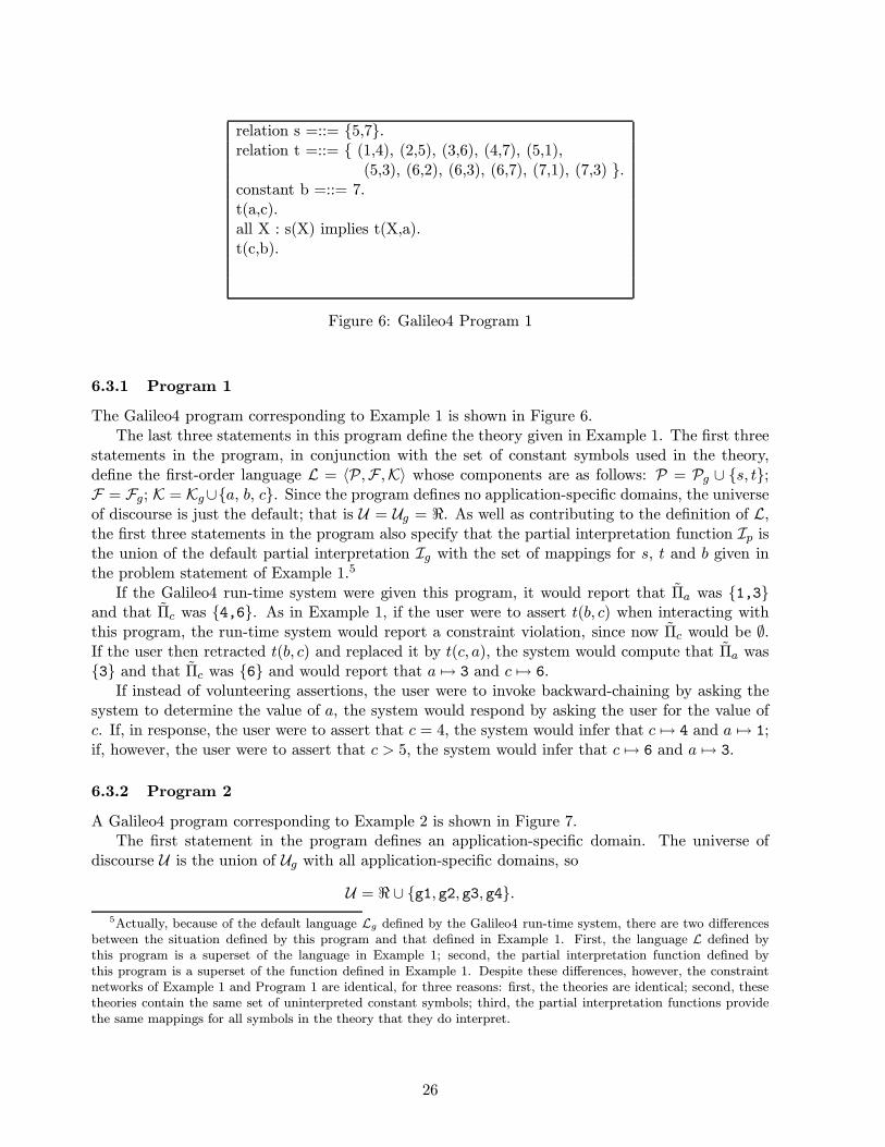
relation s =::= {5,7}.relation t =::= { (1,4), (2,5), (3,6), (4,7), (5,1),

(5,3), (6,2), (6,3), (6,7), (7,1), (7,3) }.constant b =::= 7.t(a,c).all X : s(X) implies t(X,a).t(c,b).

Figure 6: Galileo4 Program 1

6.3.1 Program 1

The Galileo4 program corresponding to Example 1 is shown in Figure 6.The last three statements in this program define the theory given in Example 1. The first three

statements in the program, in conjunction with the set of constant symbols used in the theory,define the first-order language L = 〈P,F ,K〉 whose components are as follows: P = Pg ∪ {s, t};F = Fg; K = Kg∪{a, b, c}. Since the program defines no application-specific domains, the universeof discourse is just the default; that is U = Ug = <. As well as contributing to the definition of L,the first three statements in the program also specify that the partial interpretation function Ip isthe union of the default partial interpretation Ig with the set of mappings for s, t and b given inthe problem statement of Example 1.5

If the Galileo4 run-time system were given this program, it would report that Π̃a was {1,3}and that Π̃c was {4,6}. As in Example 1, if the user were to assert t(b, c) when interacting withthis program, the run-time system would report a constraint violation, since now Π̃c would be ∅.If the user then retracted t(b, c) and replaced it by t(c, a), the system would compute that Π̃a was{3} and that Π̃c was {6} and would report that a 7→ 3 and c 7→ 6.

If instead of volunteering assertions, the user were to invoke backward-chaining by asking thesystem to determine the value of a, the system would respond by asking the user for the value ofc. If, in response, the user were to assert that c = 4, the system would infer that c 7→ 4 and a 7→ 1;if, however, the user were to assert that c > 5, the system would infer that c 7→ 6 and a 7→ 3.

6.3.2 Program 2

A Galileo4 program corresponding to Example 2 is shown in Figure 7.The first statement in the program defines an application-specific domain. The universe of

discourse U is the union of Ug with all application-specific domains, so

U = < ∪ {g1, g2, g3, g4}.5Actually, because of the default language Lg defined by the Galileo4 run-time system, there are two differences

between the situation defined by this program and that defined in Example 1. First, the language L defined bythis program is a superset of the language in Example 1; second, the partial interpretation function defined bythis program is a superset of the function defined in Example 1. Despite these differences, however, the constraintnetworks of Example 1 and Program 1 are identical, for three reasons: first, the theories are identical; second, thesetheories contain the same set of uninterpreted constant symbols; third, the partial interpretation functions providethe same mappings for all symbols in the theory that they do interpret.

26

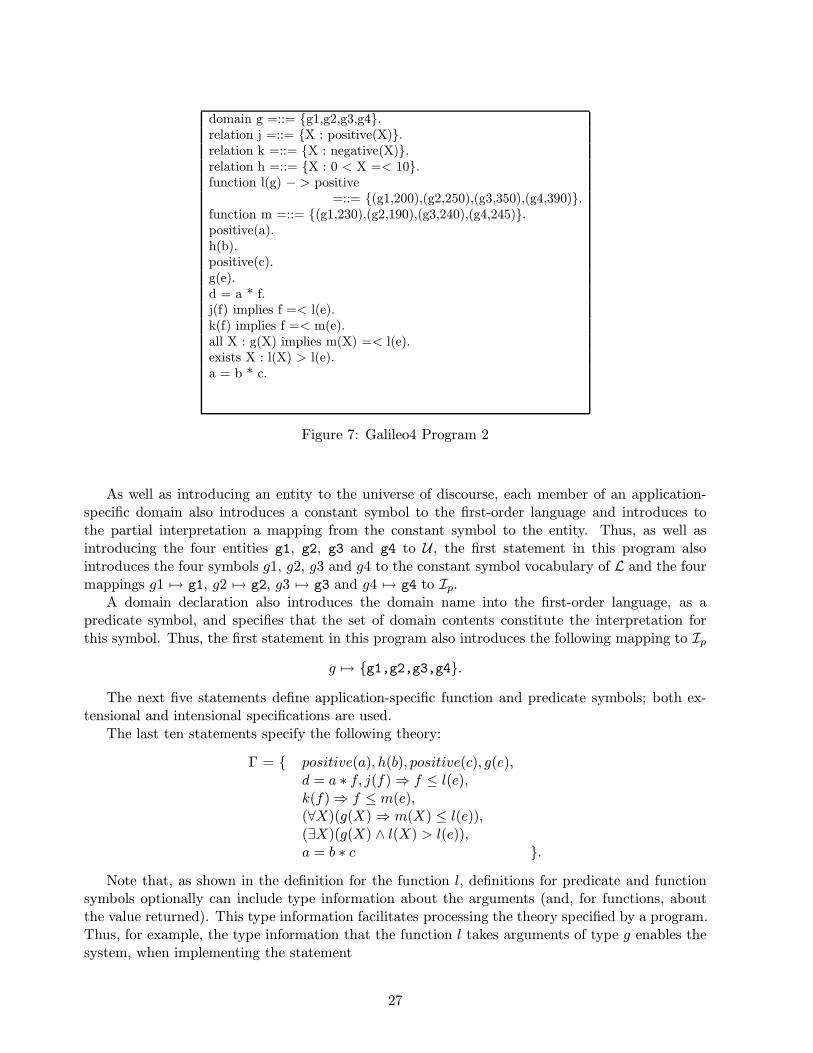
domain g =::= {g1,g2,g3,g4}.relation j =::= {X : positive(X)}.relation k =::= {X : negative(X)}.relation h =::= {X : 0 < X =< 10}.function l(g) − > positive

=::= {(g1,200),(g2,250),(g3,350),(g4,390)}.function m =::= {(g1,230),(g2,190),(g3,240),(g4,245)}.positive(a).h(b).positive(c).g(e).d = a * f.j(f) implies f =< l(e).k(f) implies f =< m(e).all X : g(X) implies m(X) =< l(e).exists X : l(X) > l(e).a = b * c.

Figure 7: Galileo4 Program 2

As well as introducing an entity to the universe of discourse, each member of an application-specific domain also introduces a constant symbol to the first-order language and introduces tothe partial interpretation a mapping from the constant symbol to the entity. Thus, as well asintroducing the four entities g1, g2, g3 and g4 to U , the first statement in this program alsointroduces the four symbols g1, g2, g3 and g4 to the constant symbol vocabulary of L and the fourmappings g1 7→ g1, g2 7→ g2, g3 7→ g3 and g4 7→ g4 to Ip.

A domain declaration also introduces the domain name into the first-order language, as apredicate symbol, and specifies that the set of domain contents constitute the interpretation forthis symbol. Thus, the first statement in this program also introduces the following mapping to Ip

g 7→ {g1,g2,g3,g4}.

The next five statements define application-specific function and predicate symbols; both ex-tensional and intensional specifications are used.

The last ten statements specify the following theory:

Γ = { positive(a), h(b), positive(c), g(e),d = a ∗ f, j(f)⇒ f ≤ l(e),k(f)⇒ f ≤ m(e),(∀X)(g(X) ⇒ m(X) ≤ l(e)),(∃X)(g(X) ∧ l(X) > l(e)),a = b ∗ c }.

Note that, as shown in the definition for the function l, definitions for predicate and functionsymbols optionally can include type information about the arguments (and, for functions, aboutthe value returned). This type information facilitates processing the theory specified by a program.Thus, for example, the type information that the function l takes arguments of type g enables thesystem, when implementing the statement

27

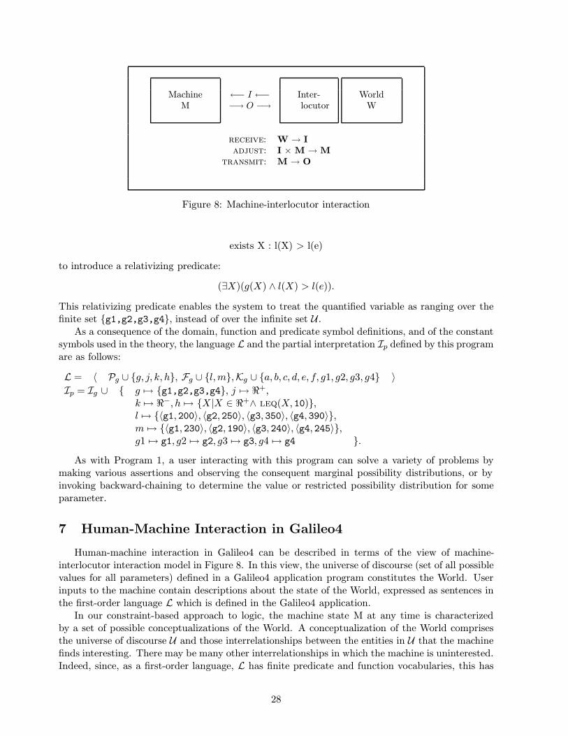
MachineM

←− I ←−−→ O −→

Inter-locutor

WorldW

receive: W → Iadjust: I ×M →M

transmit: M → O

Figure 8: Machine-interlocutor interaction

exists X : l(X) > l(e)

to introduce a relativizing predicate:

(∃X)(g(X) ∧ l(X) > l(e)).

This relativizing predicate enables the system to treat the quantified variable as ranging over thefinite set {g1,g2,g3,g4}, instead of over the infinite set U .

As a consequence of the domain, function and predicate symbol definitions, and of the constantsymbols used in the theory, the language L and the partial interpretation Ip defined by this programare as follows:

L = 〈 Pg ∪ {g, j, k, h}, Fg ∪ {l,m},Kg ∪ {a, b, c, d, e, f, g1, g2, g3, g4} 〉Ip = Ig ∪ { g 7→ {g1,g2,g3,g4}, j 7→ <+,

k 7→ <−, h 7→ {X|X ∈ <+∧ leq(X, 10)},l 7→ {〈g1, 200〉, 〈g2, 250〉, 〈g3, 350〉, 〈g4, 390〉},m 7→ {〈g1, 230〉, 〈g2, 190〉, 〈g3, 240〉, 〈g4, 245〉},g1 7→ g1, g2 7→ g2, g3 7→ g3, g4 7→ g4 }.

As with Program 1, a user interacting with this program can solve a variety of problems bymaking various assertions and observing the consequent marginal possibility distributions, or byinvoking backward-chaining to determine the value or restricted possibility distribution for someparameter.

7 Human-Machine Interaction in Galileo4

Human-machine interaction in Galileo4 can be described in terms of the view of machine-interlocutor interaction model in Figure 8. In this view, the universe of discourse (set of all possiblevalues for all parameters) defined in a Galileo4 application program constitutes the World. Userinputs to the machine contain descriptions about the state of the World, expressed as sentences inthe first-order language L which is defined in the Galileo4 application.

In our constraint-based approach to logic, the machine state M at any time is characterizedby a set of possible conceptualizations of the World. A conceptualization of the World comprisesthe universe of discourse U and those interrelationships between the entities in U that the machinefinds interesting. There may be many other interrelationships in which the machine is uninterested.Indeed, since, as a first-order language, L has finite predicate and function vocabularies, this has

28

to be the case when U is infinite: the number of possible q-ary relations between the entities of Uis 2|U|

q.

If the machine has a total model M = 〈U ,I〉 for the language L, (that is, if I provides amapping for each symbol in the union of the symbol vocabularies in L) then the machine knowseverything worth knowing about (that is, it has a total conceptualization of) the World.

Giving inputs to the machine about the state of the World has a purpose only if the machinedoes not know all the interrelationships that exist between the entities of U , that is, if the machinedoes not have a total model of the language L or if its model is not an accurate depiction of thestate of the World.

When the machine does not have a total model for L, the state of the machine (the set ofpossible conceptualizations of the World) is the set of possible models for L. That is, if at sometime t the machine’s partial model of L is M = 〈U ,It〉 then the machine state Mt is the set ofall total models M = 〈U ,I〉 for L, It ⊂ I, which are consistent with the information about thestate of the World that the machine has been given. Thus, if at time t the information that themachine has been given about the state of the World is a set Γt of sentences, then the state Mt ofthe machine is the set of all total models 〈U ,I〉, It ⊂ I, which are consistent with the truth of allsentences in Γt.

Since the state of the World, or the interlocutor’s perception of it, may change, the informationabout the World which the machine is given may not be monotonic. One input to the machine maysay that a certain sentence γ of L should be taken as true and a later input may say that γ shouldno longer be taken as true. This means that the inputs to the machine are not sentences of L;rather, they are about sentences of L. The two inputs just mentioned could not be just γ and ¬γ;that would lead to a contradiction in the theory that the machine has about the World. Rather,the two inputs must be meta-level sentences, which might be expressed imperatively as assert γand retract γ or declaratively as Γt+1 = Γt ∪ {γ} and Γt+2 = Γt+1 − {γ} = Γt.

This form of machine-interlocutor interaction is what happens when a user interacts with aGalileo4 application program. The program defines the language L, the universe of discourse Uand an initial partial interpretation Ip. The program also primes the machine with an initial set Γof L sentences about the World.

8 Summary

In this chapter, we have introduced a generalized notion of constraint processing. We have shownthat this generalized notion corresponds to a class of modeling problem in logic. We have then usedthis correspondence as the theoretical basis for a computational approach to supporting the fullfirst-order predicate calculus as a knowledge representation language. In this approach, constraintpropagation is used to treat inference as semantic entailment rather than syntactic theorem-proving.

We have introduced Galileo4, a new constraint programming language based on these ideas andshown how short constraint-based application programs can have high problem-solving versatility.

We have discussed a new algorithm for constraint propagation which generalizes and integratesseveral of the best existing techniques. The algorithm interleaves local propagation of knownstates with forms of arc and path consistency which have been generalized to infinite domains andconstraints of arbitrary arity. In the case of infinite domains, semantic reductions are used forentailment. However, we regard this algorithm as only the first in a sequence of progressively morecompetent and efficient algorithms. We regard Galileo4 as a test-bed for further developments inthis area. Although no terminating constraint propagation algorithm can ever be both sound andcomplete for the full first-order predicate calculus, an incomplete algorithm is adequate for some

29

applications, as we have illustrated by means of examples from the realms of design for testabilityand equipment selection.

We have shown how the man-machine interface presented by Galileo4 is a special case of Nilsson’sview of machine-world interaction. We believe that the lexical economy offered by the full first-orderpredicate calculus and the problem-solving versatility offered by a constraint-based approach toinference mean that the generalized form of constraint-based programming that we have introducedin this chapter is destined to become the declarative paradigm of choice.

However, this constraint-based approach to supporting the full first-order predicate calculusis still relatively immature and much remains to be done. Notable open problems include: thedevelopment of constraint propagation algorithms which are more efficient and which computebetter approximations to the true intent of infinite domain constraint networks; extending theobject-level language to include modal operators; supporting application-specific sets of reductionsand the use of results such as the Knuth-Bendix theorem [18] to compute complete reduction setsfrom the application-specific sets proposed by application programmers.

Several other related issues also present themselves. One involves the extension of the constraint-based approach to problems having non-scalar universes of discourse, where constant symbols canbe interpreted to sets or sequences; work here might include looking at issues of non-monotonicinference. Other work might be directed at using second-order and meta-level notions to ease theprogramming of large-scale applications. The specification of partial interpretations can be easedby allowing the interpretations of predicate symbols to be specified as the reflexive, symmetric, ortransitive closures of interpretations for other symbols. The specification of a theory in a program,or of augmentations to the theory by a user, can be eased by using meta-level notions to allow thesetheories and augmentations to be specified intensionally rather than extensionally; in addition,using such meta-level notions in a constraint-based approach to logic makes it possible to treat (thedeclarative aspects of) frame-based programming as a special case of theory specification.

References

[1] Bledsoe, W. (1977) Non-resolution Theorem Proving. Artificial Intelligence, 9, 1-35.

[2] Bowen, J. and Bahler, D. (1991) Conditional Existence of Variables in Generalized Constraint Networks.Proc. 9th. Nat. Conf. on Artificial Intelligence (AAAI-91), 215-220.

[3] Bowen, J. and Bahler, D. (1991) Supporting Cooperation between Multiple Perspectives in a Constraint-based approach to Concurrent Engineering. Journal of Design & Manufacturing, 1, 89-105.

[4] Bowen, J. and Bahler, D. (1992) Frames, quantification, perspectives and negotiation in constraintnetworks for life-cycle engineering. Int. Journal of AI in Engineering, 7, 199-226.

[5] Bowen, J. and Bahler, D. (1993) Constraint-Based Software for Concurrent Engineering. IEEE Com-puter, Special Issue on Computer Support for Concurrent Engineering, 26 (1), 66-68.

[6] Borning, A. (1981) The Programming Language Aspects of ThingLab, A Constraint-Oriented Simula-tion Laboratory. ACM Trans. on Prog. Lang. and Sys., 3 (4), 353-387.

[7] Chronaki, C. and Baldwin, D. (1990) A Front End for CONSUL. Technical Report 319, Department ofComputer Science, University of Rochester.

[8] Colmerauer, A. (1990) An Introduction to Prolog III. Commun. ACM, 28 (4), 412-418.

[9] Davis, E. (1987) Constraint Propagation with Interval Labels. Artificial Intelligence, 32, 281-331.

[10] Dechter, R. (1990) Enhancement Schemes for Constraint Processing: Backjumping, Learning, andCutset Decomposition. Artificial Intelligence, 41, 273-312.

30

[11] Dincbas, M., van Hentenryck, P., Simonis, H., Aggoun, A., Graf, T. and Berthier, F. (1988) TheConstraint Logic Programming Language CHIP. Proc. Fifth Gen. Comp. Sys. ’88.

[12] Faltings, B. (1994) Arc-consistency for continuous variables. Artificial Intelligence, 65 (2), 363-376.

[13] Freuder, E. (1982) A Sufficient Condition for Backtrack-free Search. Journal of the ACM, 29 (1), 24-32.

[14] Gosling, J. (1983) Algebraic Constraints. Technical Report CS-83-132, Carnegie-Mellon University,Pittsburgh.

[15] Han, C.-C. and Lee, C.-H. (1988) Comments on Mohr and Henderson’s Path Consistency Algorithm.Artificial Intelligence, 36, 125-130.

[16] Haralick, R. and Elliot, G. (1980) Increasing Tree Search Efficiency for Constraint Satisfaction Problems.Artificial Intelligence, 14, 263-313.

[17] Jaffar, J., Michaylov, S., Stuckey, P., and Yap, R. (1992) The CLP(<) Language and System. ACMTrans. on Prog. Lang. and Systems, 14 (3), 339-395.

[18] Knuth, D.and Bendix, P. (1970) Simple Word Problems in Universal Algebras. in Computational Prob-lems in Abstract Algebra, (ed. J. Leech), Pergamon Press, New York.

[19] Lambert, K.and van Fraassen, B. (1972) Derivation and Counterexample: An Introduction to Philo-sophical Logic, Dickenson Publishing Company, Enrico, CA.

[20] Leler. W. (1988) Constraint Programming Languages, Addison-Wesley, Reading, MA.

[21] Mackworth, A. (1977) Consistency in Networks of Relations. Artificial Intelligence, 8, 99-118.

[22] Maher, M. and Stuckey, P. (1989) Expanding Query Power in Constraint Programming Languages.Proc. North American Conf. on Logic Programming, 20-36.

[23] Mittal, S. and Falkenhainer, B. (1990) Dynamic Constraint Satisfaction Problems. Proc. 8th. Nat. Conf.on Artificial Intelligence (AAAI-90), 25-32.

[24] Mohr, R. and Henderson, T. (1986) Arc and Path Consistency Revisited. Artificial Intelligence, 28,225-233.

[25] Nadel, B. (1989) Constraint Satisfaction Algorithms. Computational Intelligence, 5 (4), 188-224.

[26] Nilsson, N. (1991) Logic and artificial intelligence. Artificial Intelligence, 47, 31-56.

[27] Paramasivam, M. (1991) An Axiom Based Approach to Constraint Satisfaction. M.S. Thesis, ComputerScience Department, North Carolina State University, Raleigh.

[28] Sussman, G. and Steele, G. (1980) Constraints: A Language for Expressing Almost-Hierarchical De-scriptions. Artificial Intelligence, 14, 1-39.

[29] Sutherland, I. (1963) SKETCHPAD: A Man-Machine Graphical Communication System. Proc. SpringJoint Comp. Conf., IFIPS.

31

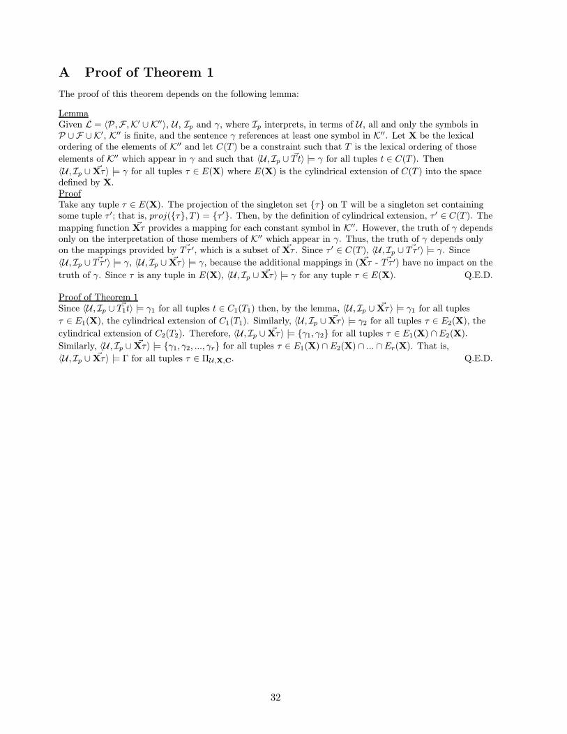
A Proof of Theorem 1

The proof of this theorem depends on the following lemma:

LemmaGiven L = 〈P ,F ,K′ ∪ K′′〉, U , Ip and γ, where Ip interprets, in terms of U , all and only the symbols inP ∪ F ∪K′, K′′ is finite, and the sentence γ references at least one symbol in K′′. Let X be the lexicalordering of the elements of K′′ and let C(T ) be a constraint such that T is the lexical ordering of those

elements of K′′ which appear in γ and such that 〈U , Ip ∪ ~T t〉 |= γ for all tuples t ∈ C(T ). Then

〈U , Ip ∪ ~Xτ〉 |= γ for all tuples τ ∈ E(X) where E(X) is the cylindrical extension of C(T ) into the spacedefined by X.ProofTake any tuple τ ∈ E(X). The projection of the singleton set {τ} on T will be a singleton set containingsome tuple τ ′; that is, proj({τ}, T ) = {τ ′}. Then, by the definition of cylindrical extension, τ ′ ∈ C(T ). The

mapping function ~Xτ provides a mapping for each constant symbol in K′′. However, the truth of γ dependsonly on the interpretation of those members of K′′ which appear in γ. Thus, the truth of γ depends onlyon the mappings provided by ~T τ ′, which is a subset of ~Xτ . Since τ ′ ∈ C(T ), 〈U , Ip ∪ ~T τ ′〉 |= γ. Since

〈U , Ip ∪ ~T τ ′〉 |= γ, 〈U , Ip ∪ ~Xτ〉 |= γ, because the additional mappings in ( ~Xτ - ~T τ ′) have no impact on the

truth of γ. Since τ is any tuple in E(X), 〈U , Ip ∪ ~Xτ〉 |= γ for any tuple τ ∈ E(X). Q.E.D.

Proof of Theorem 1Since 〈U , Ip ∪ ~T1t〉 |= γ1 for all tuples t ∈ C1(T1) then, by the lemma, 〈U , Ip ∪ ~Xτ〉 |= γ1 for all tuples

τ ∈ E1(X), the cylindrical extension of C1(T1). Similarly, 〈U , Ip ∪ ~Xτ〉 |= γ2 for all tuples τ ∈ E2(X), the

cylindrical extension of C2(T2). Therefore, 〈U , Ip ∪ ~Xτ〉 |= {γ1, γ2} for all tuples τ ∈ E1(X) ∩E2(X).

Similarly, 〈U , Ip ∪ ~Xτ〉 |= {γ1, γ2, ..., γr} for all tuples τ ∈ E1(X) ∩ E2(X) ∩ ... ∩ Er(X). That is,

〈U , Ip ∪ ~Xτ〉 |= Γ for all tuples τ ∈ ΠU ,X,C. Q.E.D.

32