Computational Neuroscience SummerProgram: Introductory Course

May 31 – June 3, 2011

Instructors: Dr. Joshua Jacobs (joshua.jacobs@drexel.edu)

Dr. Jeremy Manning (manning3@mail.med.upenn.edu)

Suggested texts: Theoretical Neuroscience, Dayan and Abbott

Principles of Neural Science, Kandel, Schwartz, and Jessell

Matlab for Neuroscientists, Wallisch et al.

Course overview: This intensive introductory course is intended to familiarize students withbasic techniques in computational modeling and analysis of neural data using Matlab. Studentsmay (and are encouraged to) work together on assignments, but each student will be expectedto hand in their own work. Assignments will be reviewed, but no formal grades will be assigned.

Course Outline:

Orientation and ethics training . . . . . . . . . . . . . . . . . . . . . . . . . . . . . . . May 31 (AM)Introduction to programming in Matlab . . . . . . . . . . . . . . . . . . . . . . May 31 (PM)Introduction to computational modeling . . . . . . . . . . . . . . . . . . . . . . . June 1 (AM)Integrate-and-fire neuron model . . . . . . . . . . . . . . . . . . . . . . . . . . . . . . . June 1 (PM)Hodgkin-Huxley neuron model . . . . . . . . . . . . . . . . . . . . . . . . . . . . . . . . June 2 (AM)Extensions of the Hodgkin-Huxley model . . . . . . . . . . . . . . . . . . . . . . June 2 (PM)Neural data processing techniques . . . . . . . . . . . . . . . . . . . . . . . . . . . . . June 3 (AM)Open lab time . . . . . . . . . . . . . . . . . . . . . . . . . . . . . . . . . . . . . . . . . . . . . . . . .June 3 (PM)

Note: The above course outline is approximate and is subject to change pending students’needs and interests. Because of the brief duration of this course, we are only able to provide asmall “taste” of the diverse and evolving field of computational neuroscience. Students seekingmore in-depth coverage of computational neuroscience, including the topics discussed in thiscourse, are encouraged to read the suggested texts.

MATLAB Cheat Sheet

Basic Commands

% Indicates rest of line is commented out.; If used at end of command it suppresses output.

If used within matrix definitions it indicates the end of a row.save filename Saves all variables currently in workspace to file filename.mat.save filename x y z Saves x, y, and z to file filename.mat.save -append filename x Appends file filename.mat by adding x.load filename Loads variables from file filename.mat to workspace.! Indicates that following command is meant for the operating system.... Indicates that command continues on next line.help function/command Displays information about the function/command.clear Deletes all variables from current workspace.clear all Basically same as clear.clear x y Deletes x and y from current workspace.home Moves cursor to top of command window.clc Homes cursor and clears command window.close Closes current figure window.close all Closes all open figure windows.close(H) Closes figure with handle H.global x y Defines x and y as having global scope.keyboard When placed in an M-file, stops execution of the file and gives

control to the user’s keyboard. Type return to return controlto the M-file or dbquit to terminate program.

A=xlsread(‘data’,... Sets A to be a 5-by-2 matrix of the data contained in‘sheet1’,‘a3:b7’) cells A3 through B7 of sheet sheet1 of excel file data.xlsSucces=xlswrite(... Writes contents of A to sheet sheet1 of excel file‘results’,A,‘sheet1’,‘c7’) results.xls starting at cell C7. If successful success= 1.

path Display the current search path for .m filesaddpath c:\my_functions Adds directory c:\my_functions to top of current search path.rmpath c:\my_functions Removes directory c:\my_functions from current search path.disp(’random statement’) Prints random statement in the command window.disp(x) Prints only the value of x on command window.disp([’x=’,num2str(x,5)]) Displays x= and first 5 digits of x on command window. Only works

when x is scalar or row vector.fprintf(...

Displays The 3 is 1.73. on command window.’The %g is %4.2f.\n’, x,sqrt(x))

format short Displays numeric values in floating point format with 4 digits afterthe decimal point.

format long Displays numeric values in floating point format with 15 digits afterthe decimal point.

Plotting Commands

figure(H) Makes H the current figure. If H does not exist is creates H.

1

Note that H must be a positive integer.plot(x,y) Cartesian plot of x versus y.plot(y) Plots columns of y versus their index.plot(x,y,‘s’) Plots x versus y according to rules outlined by s.semilogx(x,y) Plots log(x) versus y.semilogy(x,y) Plots x versus log(y).loglog(x,y) Plots log(x) versus log(y).grid Adds grid to current figure.title(‘text’) Adds title text to current figure.xlabel(‘text’) Adds x-axis label text to current figure.ylabel(‘text’) Adds y-axis label text to current figure.hold on Holds current figure as is so subsequent plotting commands add

to existing graph.hold off Restores hold to default where plots are overwritten by new plots.

Creating Matrices/Special Matrices

A=[1 2;3 4] Defines A as a 2-by-2 matrix where the first row contains thenumbers 1, 2 and the second row contains the number 3, 4.

B=[1:1:10] Defines B as a vector of length 10 that contains the numbers1 through 10.

A=zeros(n) Defines A as an n-by-n matrix of zeros.A=zeros(m,n) Defines A as an m-by-n matrix of zeros.A=ones(n) Defines A as an n-by-n matrix of ones.A=ones(n,m) Defines A as an m-by-n matrix of ones.A=eye(n) Defines A as an n-by-n identity matrix.A=repmat(x,m,n) Defines A as an m-by-n matrix in which each element is x.

linspace(x1, x2, n) Generates n points between x1 and x2.Matrix Operations

A*B Matrix multiplication. Number of columns of A must equal numberof rows of B.

Aˆn A must be a square matrix. If n is an integer and n > 1 than Aˆn isA multiplied with itself n times. Otherwise, Aˆn is the solution toAnvi = livi where li is an eigenvalue of A and vi is the correspondingeigenvector.

A/B This is equivalent to A*inv(B) but computed more efficiently.A\B This is equivalent to inv(A)*B but computed more efficiently.A.*B,A./B, Element-by-element operations.A.\B,A.ˆn

A’ Returns the transpose of A.inv(A) Returns the inverse of A.length(A) Returns the larger of the number of rows and columns of A.size(A) Returns of vector that contains the dimensions of A.size(A,1) Returns the number of rows in A.reshape(A,m,n) Reshapes A into an m-by-n matrix.

2

kron(A,B) Computes the Kronecker tensor product of A with B.A = [A X] Concatenates the m-by-n matrix A by adding the m-by-k matrix X as

additional columns.A = [A; Y] Concatenates the m-by-n matrix A by adding the k-by-n vector Y as

additional rows.

Data Analysis Commands

rand(m,n) Generates an m-by-n matrix of uniformly distributed random numbers.randn(m,n) Generates an m-by-n matrix of normally distributed random numbers.max(x) If x is a vector it returns the largest element of x.

If x is a matrix it returns a row vector of the largest element in eachcolumn of x.

min(x) Same as max but returns the smallest element of x.mean(x) If x is a vector it returns the mean of the elements of x.

If x is a matrix it returns a row vector of the means for each column of x.sum(x) If x is a vector it returns the sum of the elements of x.

If x is a matrix it returns a row vector of the sums for each column of x.prod(x) Same as sum but returns the product of the elements of x.std(x) If x is a vector it returns the standard deviation of the elements of x.

If x is a matrix it returns a row vector of the standard deviations for eachcolumn of x.

var(x) Same as std but returns the variance of the elements of x.

Conditionals and Loops

for i=1:10

procedure Iterates over procedure incrementing i from 1 to 10 by 1.end

while(criteria)

procedure Iterates over procedure as long as criteria is true.end

if(criteria 1)

If criteria 1 is true do procedure

1, else if criteria 2 is true doprocedure 2, else do procedure 3.

procedure 1

elseif(criteria 2)

procedure 2

else

procedure 3

end

3

Problem Set 1 -- Introduction to programming in Matlab

Computational Neuroscience Summer Program

May, 2011

Log into the computer with your PennKey and start Matlab. Please put your answers to this assignment in a single Microsoft Word document. This document should include your raw Matlab code, the commands you type to run the code, and its output text and plots.

Some of these questions require functions that you may not have seen before. If you have questions, please ask the instructors and feel free to consult Matlabʼs great built-in help functions and online tutorials at mathworks.com.

1.! ConcatenationWrite a script that creates the variables a = [1 2 3], b = 4, c = 5, d = [6; 9], e = [7 8]. Use only these variables to create the matrix m = [1 2 3; 4 5 6; 7 8 9] in a single line of code through horizontal & vertical concatenation. (Hint: use nested [ ] operations.) Now change the script into a function. What is the effective difference between calling the script and the function?

2.! Number ClassificationWrite a function that will indicate whether an input number is negative, positive, or zero, as well as even or odd. The function should print these results to the command window and not return anything.

3.! For loopWrite a function that creates a Fibonacci sequence (a series of numbers where each element is the sum of the previous two elements; youʼll have to start it with [1 1]). It should have an input parameter that indicates the desired length of the output sequence.

4. PlottingDownload this file and load it into matlab: # http://memory.psych.upenn.edu/~josh/Q4.matPlot the variable ʻZʼ from this file using the standard plot command.

Next, create a function plot_labeled_peak that accepts one input vector. It should plot the vector in black. In addition, the largest data point in this vector should be labeled with a red circle, and the smallest data point should be labeled with a blue ʻxʼ. Show the result of this function when plotting ʻZʼ.

5. Challenge questions: Performance analysisA.Here we are interested in calculating the lengths of many three-element vectors according to the pythagorean theorem (i.e., sqrt(a2 + b2 + c2)). Write a function that takes a three-column matrix, and returns the length of the vector in each row using a loop. Use randn to create random three-column matrices with 10, 100, 1000, & 10000 rows, and measure how long it takes your function to compute each one. Next, create a similar function that does the same calculations in a vectorized fashion. Compare the performance of the two by plotting the execution times of each of the two functions versus the number of rows in the matrix.

B.In Matlab, preallocating a vector in a single command (by using the ʻzerosʼ or ʻonesʼ functions, for example) can make things operate much more quickly than repeatedly appending individual elements to the end of a matrix. Write a version of the Fibonacci function from Question 3 that preallocates the output. How fast does it calculate a 20,000 element Fibonacci sequence? How does this speed compare to the previous version of this function? Plot the Fibonacci execution times of various sequence lengths, for both versions of this procedure.

C.A common data analysis tool is to normalize a dataset so that it has a mean of zero and a standard deviation of 1. Here is a function that takes in a large matrix and returns a normalized dataset where each row has a mean of zero and a standard deviation of 1:

function x=normData_loop(x)for row=1:size(x,1) m=mean(x(row,:)); s=std(x(row,:)); x(row,:)=(x(row,:)-m)/s;end

Can you write a vectorized version of this function? (Hint: use repmat.) How does the execution time of your function compare with normData_loop on a 1000 by 1000 matrix (e.g., rand(1000,1000))?

Lecture 2 – Introduction to computational modeling

Computational Neuroscience Summer Program

June, 2011

Motivation. This lecture is intended to give students a general intuition for basic mathematical lan-guage used to describe and model neurons. These principles will serve as the foundation for futurelectures.

Basic organization of the brain. The brain is typically divided into 4 lobes. The temporal lobe containsneural machinery for processing speech and sounds, spatial information, and for encoding episodic(autobiographical) memories. The parietal lobe is involved with sensory perception, sensory integration,and memory. The frontal lobe is associated with personality, reasoning, planning, problem solving, work-ing memory, and movement. The occipital lobe is primiarily involved with vision and visual processing.The central sulcus separates the primary motor cortex (frontal lobe) from the primary somatosensorycortex (parietal lobe). The medial longitudinal fissure’ separates the right and left hemispheres of thebrain. The spinal cord sends signals from the primary motor cortex to the body’s skeletal muscles.

Neuron anatomy. Neurons are electrically excitable cells in the brain. Neurons “listen” to other cellsvia branch-like dendrites. Signals from the dendrites travel down to the cell body, or soma, which containsthe nucleus of the cell. Neurons communicate with other cells by sending electrical impulses downtheir axons, which most often synapse onto the dendrites of other neurons.

Action potentials. Neurons communicate with each other by changes in their membrane voltage(we’ll get to what this means in a bit). Small changes in membrane voltage are picked up by neuronsup to approximately 1 mm away. Thus, for nervous systems on the scale of 1 mm, such as the fruitfly nervous system, no other special mode of communication is needed. However, in larger nervoussystems (e.g. ours), neurons fire action potentials – sudden changes in voltage. These form the basicmode of neural communication in the brain. Over the next few lectures we’ll be trying to understandhow action potentials come about by modeling neurons in increasing levels of detail.

The neuron as a fluid-filled ball. Each µm3 of cytoplasm contains on the order of 1010 water molecules,108 ions (e.g. sodium, potassium, calcium, chloride), 107 small molecules (e.g. amino acids, nucleicacids), and 105 proteins. Relative to the extracellular space, the inside of the cell is negatively charged(the difference is carried by about 1 out of every 100,000 ions). This results in a voltage (V) across themembrane of approximately -70 mV.

1

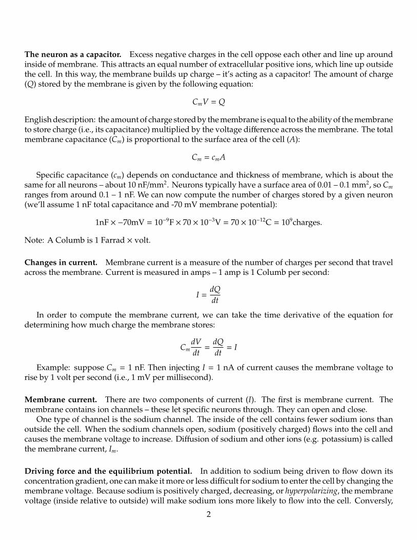
The neuron as a capacitor. Excess negative charges in the cell oppose each other and line up aroundinside of membrane. This attracts an equal number of extracellular positive ions, which line up outsidethe cell. In this way, the membrane builds up charge – it’s acting as a capacitor! The amount of charge(Q) stored by the membrane is given by the following equation:

CmV = Q

English description: the amount of charge stored by the membrane is equal to the ability of the membraneto store charge (i.e., its capacitance) multiplied by the voltage difference across the membrane. The totalmembrane capacitance (Cm) is proportional to the surface area of the cell (A):

Cm = cmA

Specific capacitance (cm) depends on conductance and thickness of membrane, which is about thesame for all neurons – about 10 nF/mm2. Neurons typically have a surface area of 0.01 – 0.1 mm2, so Cm

ranges from around 0.1 – 1 nF. We can now compute the number of charges stored by a given neuron(we’ll assume 1 nF total capacitance and -70 mV membrane potential):

1nF × −70mV = 10−9F × 70 × 10−3V = 70 × 10−12C = 109charges.

Note: A Columb is 1 Farrad × volt.

Changes in current. Membrane current is a measure of the number of charges per second that travelacross the membrane. Current is measured in amps – 1 amp is 1 Columb per second:

I =dQdt

In order to compute the membrane current, we can take the time derivative of the equation fordetermining how much charge the membrane stores:

CmdVdt

=dQdt

= I

Example: suppose Cm = 1 nF. Then injecting I = 1 nA of current causes the membrane voltage torise by 1 volt per second (i.e., 1 mV per millisecond).

Membrane current. There are two components of current (I). The first is membrane current. Themembrane contains ion channels – these let specific neurons through. They can open and close.

One type of channel is the sodium channel. The inside of the cell contains fewer sodium ions thanoutside the cell. When the sodium channels open, sodium (positively charged) flows into the cell andcauses the membrane voltage to increase. Diffusion of sodium and other ions (e.g. potassium) is calledthe membrane current, Im.

Driving force and the equilibrium potential. In addition to sodium being driven to flow down itsconcentration gradient, one can make it more or less difficult for sodium to enter the cell by changing themembrane voltage. Because sodium is positively charged, decreasing, or hyperpolarizing, the membranevoltage (inside relative to outside) will make sodium ions more likely to flow into the cell. Conversly,

2

increasing, or depolarizing, the membrane voltage will make sodium ions less likely to flow into the cell.The membrane potential at which net flow of an ion stops is called the equilibrium potential, E. WhenV > E, positive ions flow out of the cell. When V < E, positive ions flow into the cell. This means thatV is driven towards E. Thus, we sometimes refer to the quantity (V − E) as the driving force across thecell membrane. When the driving force is negative, positive ions are driven out of the cell. When thedriving force is positive, positive ions are pulled into the cell.

External current. The second component of current is current that is injected into the neuron fromexternal sources (e.g. if we stick an electrode into the neuron and pump in current).

The change in membrane voltage V due to some change in current I follows Ohm’s Law:

V = IR,

where R is the membrane resistance, described next.

Membrane resistance. Ion channels are like little holes in the membrane. They let ions pass throughthem – i.e., they conduct ions. A given unit area of membrane has some number of open channels, andwe can measure the ease with which ions pass through those channels – the specific conductance, gm.The total conducatance is proportional to the neuron’s area:

Gm = gmA

By convention, we tend to talk about the inverse of conductance, which is called resistance. Whereasconductance is proportional to the surface area of the neuron, resistance is proportional to the inverseof the surface area of the neuron:

Rm =rm

ANote that the membrane resistance often changes as a function of voltage, which makes things interesting– we’ll get to this later.

The Neuron Equation. Previously we had:

CmdVdt

= I,

which we can update to reflect that I is comprised of both membrane and external currents:

CmdVdt

= Ie + Im.

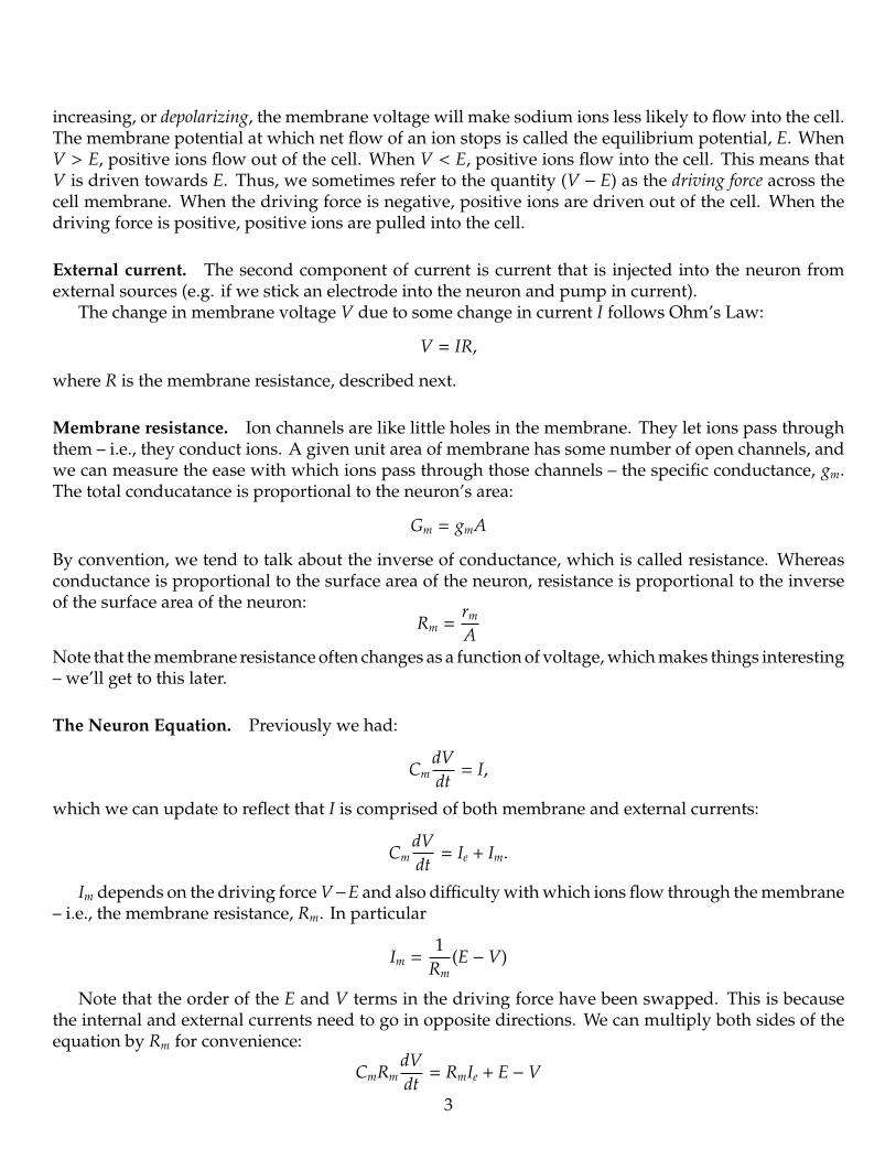
Im depends on the driving force V−E and also difficulty with which ions flow through the membrane– i.e., the membrane resistance, Rm. In particular

Im =1

Rm(E − V)

Note that the order of the E and V terms in the driving force have been swapped. This is becausethe internal and external currents need to go in opposite directions. We can multiply both sides of theequation by Rm for convenience:

CmRmdVdt

= RmIe + E − V

3

Since Cm = cmA and Rm = rmA , the A’s cancel, and we get cmrm, which is independent of the cell’s

surface area. Since cmrm determines the rate at which the cell’s membrane potential changes, it is givena special variable, τm, or the membrane time constant. The equation for all neuron models we’ll see inthis mini-course is:

τmdVdt

= RmIe + E − V

V∞. From the above equation, we see that the change in membrane voltage is some fraction (propor-tional to τm) of the difference between RmIe + E and the current membrane voltage, V. By this equationthe membrane voltage approaches RmIe + E over time. For convenience we can define

V∞ = E + RmIe,

where V∞ is the membrane voltage that will be reached given an external current and membraneresistance, and an infinite amount of time.

Resting potential. If you shut off the external current (i.e., set Ie = 0), then V∞ = E. For this reason, wecall E the resting potential of the cell – the potential the cell approaches if we remove external forces.

Computing the voltage at a particular time, t. We need to solve the following differential equationfor V:

τmdVdt

= RmIe + E − V

We know that, given enough time, V tends towards V∞, so we can say that at time t:

V(t) = V∞ + f (t)

Now we need to find f (t) (we’ll abbreviate f (t) as f for convenience). We use the equation above,substituting in V∞ + f for V:

τmd fdt

= RmIe + E − V∞ − f

Since V∞ = RmIe + E, those terms cancel and we have:

τmd fdt

= − f

soτmd f = − f dt

τmd ff

= −dt

Now that we have the f ’s and t’s on different sides of the equation, we can take the integral from 0to t of both sides: ∫ f (t)

f (0)τm

d ff

=

∫ t

0−dt

Solve the right hand side yields: ∫ f (t)

f (0)τm

d ff

= −t

4

We can solve the left hand side using the rule∫

1xdx = ln(x):

τm[ln( f (t)) − ln( f (0))] = −t

τmlnf (t)f (0)

= −t

Now we can solve for f (t):

lnf (t)f (0)

=−tτm

f (t)f (0)

= e−tτm

f (t) = f (0)e−tτm

Previously, we said that the voltage changes as a function of the distance between the voltage at thepresent time and V∞. So f (0) = V(0) − V∞, and f (t) = f (0)e

−tτm .

Plugging f (t) back into the original equation gives:

V(t) = V∞ + f (t) = V∞ + (V(0) − V∞)e−tτm

This gives us a way to compute how long it will take to charge up the neuron to an arbitrary voltageV(t), by solving for t.

Sanity checks. For t = 0, e−tτm = 1, so we get:

V(0) = V∞ + V(0) − V∞ = V(0)

When t is very large, e−tτm approaches 0, so V(t) approaches V∞.

5

Problem Set 2 – Introduction to computational modeling

Computational Neuroscience Summer Program

June, 2011

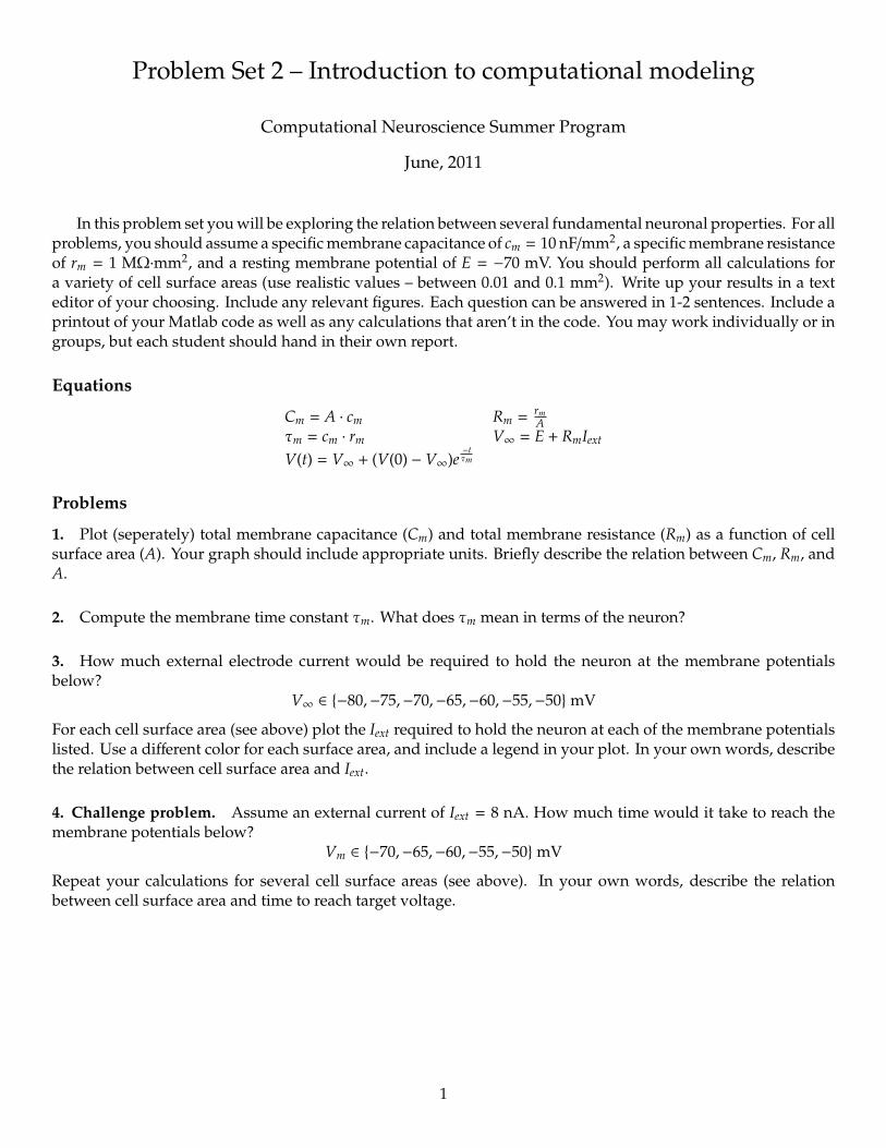
In this problem set you will be exploring the relation between several fundamental neuronal properties. For allproblems, you should assume a specific membrane capacitance of cm = 10 nF/mm2, a specific membrane resistanceof rm = 1 MΩ·mm2, and a resting membrane potential of E = −70 mV. You should perform all calculations fora variety of cell surface areas (use realistic values – between 0.01 and 0.1 mm2). Write up your results in a texteditor of your choosing. Include any relevant figures. Each question can be answered in 1-2 sentences. Include aprintout of your Matlab code as well as any calculations that aren’t in the code. You may work individually or ingroups, but each student should hand in their own report.

Equations

Cm = A · cm Rm = rmA

τm = cm · rm V∞ = E + RmIext

V(t) = V∞ + (V(0) − V∞)e−tτm

Problems

1. Plot (seperately) total membrane capacitance (Cm) and total membrane resistance (Rm) as a function of cellsurface area (A). Your graph should include appropriate units. Briefly describe the relation between Cm, Rm, andA.

2. Compute the membrane time constant τm. What does τm mean in terms of the neuron?

3. How much external electrode current would be required to hold the neuron at the membrane potentialsbelow?

V∞ ∈ −80,−75,−70,−65,−60,−55,−50mV

For each cell surface area (see above) plot the Iext required to hold the neuron at each of the membrane potentialslisted. Use a different color for each surface area, and include a legend in your plot. In your own words, describethe relation between cell surface area and Iext.

4. Challenge problem. Assume an external current of Iext = 8 nA. How much time would it take to reach themembrane potentials below?

Vm ∈ −70,−65,−60,−55,−50mV

Repeat your calculations for several cell surface areas (see above). In your own words, describe the relationbetween cell surface area and time to reach target voltage.

1

Lecture 3 – Integrate-and-fire neuron model

Computational Neuroscience Summer Program

June, 2011

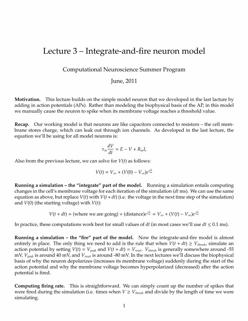
Motivation. This lecture builds on the simple model neuron that we developed in the last lacture byadding in action potentials (APs). Rather than modeling the biophysical basis of the AP, in this modelwe manually cause the neuron to spike when its membrane voltage reaches a threshold value.

Recap. Our working model is that neurons are like capacitors connected to resistors – the cell mem-brane stores charge, which can leak out through ion channels. As developed in the last lecture, theequation we’ll be using for all model neurons is:

τmdVdt= E − V + RmIe

Also from the previous lecture, we can solve for V(t) as follows:

V(t) = V∞ + (V(0) − V∞)e−tτm

Running a simulation – the “integrate” part of the model. Running a simulation entails computingchanges in the cell’s membrane voltage for each iteration of the simulation (dt ms). We can use the sameequation as above, but replace V(t) with V(t+dt) (i.e. the voltage in the next time step of the simulation)and V(0) (the starting voltage) with V(t):

V(t + dt) = (where we are going) + (distance)e−tτm = V∞ + (V(t) − V∞)e

−tτm

In practice, these computations work best for small values of dt (in most cases we’ll use dt ≤ 0.1 ms).

Running a simulation – the “fire” part of the model. Now the integrate-and-fire model is almostentirely in place. The only thing we need to add is the rule that when V(t + dt) ≥ Vthresh, simulate anaction potential by setting V(t) = Vpeak and V(t + dt) = Vreset. Vthresh is generally somewhere around -55mV, Vpeak is around 40 mV, and Vreset is around -80 mV. In the next lectures we’ll discuss the biophysicalbasis of why the neuron depolarizes (increases its membrane voltage) suddenly during the start of theaction potential and why the membrane voltage becomes hyperpolarized (decreased) after the actionpotential is fired.

Computing firing rate. This is straightforward. We can simply count up the number of spikes thatwere fired during the simulation (i.e. times when V ≥ Vthresh and divide by the length of time we weresimulating.

1

Analytic solution for firing rate. While the full integrate-and-fire simulation is often useful (and isnecessary if you want to model things like spike timing), it turns out that there is an analytic methodfor computing the expected firing rate of the model, given a constant external current Ie. We start withthe equation for finding the membrane voltage at time t:

V(t) = V∞ + (V(0) − V∞)e−tτm

We can then solve for t as follows:

V(t) − V∞ = (V(0) − V∞)e−tτm

V(t) − V∞(V(0) − V∞)

= e−tτm

ln(V(t) − V∞V(0) − V∞

) =−tτm

τmln(V(t) − V∞V(0) − V∞

) = −t

t = −τmln(V(t) − V∞V(0) − V∞

)

Now let’s suppose our model neuron has just fired a spike in the previous timestep of our simulation.We start by setting V(0) = Vreset. We next need to know how long it is until the neuron next fires aspike (the inter-spike interval, tisi – or, in other words, the time t at which V(t) = Vthresh after starting atV(0) = Vreset. Plugging in the appropriate values, we can compute tisi as follows:

tisi = −τmln(Vthresh − V∞Vreset − V∞

)

Recall that V∞ = E + RmIe. Thus

tisi = −τmln(Vthresh − (E + RmIe)Vreset − (E + RmIe)

) = −τmln(Vthresh − E − RmIe

Vreset − E − RmIe)

The firing rate (risi) is the inverse of the inter-spike interval:

risi = (−τmln(Vthresh − E − RmIe

Vreset − E − RmIe))−1

Putting it all together. To run the simulation, start with the basic model neuron equation:

τmdVdt= E − V + RmIe

Now solve for dV:dVdt=

E − V + RmIe

τm

dV = (E − V + RmIe

τm)dt

Start the simulation by setting V(0) = E. With each timestep set V(t + dt) = V(t) + dV. You’ll need tore-compute dV for each time-step given V(t) and Ie(t) for the appropriate time t. Remember to includethe rule for firing a spike (and resetting) when V > Vthresh – otherwise the neuron won’t fire spikes.

2

General MATLAB stuff. Set up your environment:

E = -70; %mV

c_m = 10; %nF / mmˆ2

r_m = 1; %M ohm * mmˆ2

A = 0.025; %mmˆ2

V_reset = -80; %mV

V_thresh = -55; %mV

V_peak = 40; %mV

dt = 0.1; %ms

t = 1:dt:1000; %ms

Now loop:

V(1) = E;

for i = 2:length(t)

if V(i-1) > V_thresh

fire a spike

else

compute dV

V(i) = V(i-1) + dV;

end

For the problem set, you should write a function that runs the integrate-and-fire model for a given setof parameters. Your function should at return the firing rate (computed numerically, not using the risi

equation). You also might want to have it return the vector of V over time, depending on how you setup your code.

3

Problem Set 3 – Integrate-and-fire neuron model

Computational Neuroscience Summer Program

June, 2011

In this problem set you will be building a simple integrate-and-fire neuron. You should assume a specificmembrane capacitance of cm = 10 nF/mm2, a specific membrane resistance of rm = 1 MΩ·mm2, a resting membranepotential of E = −70 mV, a reset potential of Vreset = −80 mV, an action potential threshold of Vthreshold = −55mV, and a cell surface area of A = 0.025 mm2. Write up your results in a text editor of your choosing. Includeany relevant figures, your Matlab code, and any other calculations related to the problem set. You may workindividually or in groups, but each student should hand in their own report.

Equations

Cm = A · cm Rm = rmA

τm = cm · rm V∞ = E + RmIext

V(t) = V∞ + (V(0) − V∞)e−tτm risi = (τmln( RmIext+E−Vreset

RmIext+E−Vthreshold))−1

τmdVdt = E − V(t − 1) + RmIext

Problems

1. Model an integrate-and-fire neuron using the equations above and the following rule: when the neuron’smembrane voltage exceeds Vthreshold, set the voltage in that timestep to Vpeak = 40 mV, and in the next timestepset the voltage to Vreset. Set dt = 0.1 ms. Apply a square pulse of 0.5 nA from t = 250 ms until t = 750 ms inyour simulation. Use Matlab’s subplot command to plot the membrane voltage over time in the top panel andIext in the bottom panel (use the same time scale for the horizontal axis of both plots). No text is required for thisquestion; just include a plot.

2. Compute the average firing rate (spikes per second) of the integrate-and-fire neuron for the pulse intervalyou used in quesion 1 (500 ms). Now plot simulated firing rate vs risi for several values of Iext (use Iext between0 and 1 nA). How does the firing rate of the modeled neuron compare to the estimated firing rate given by risi?Note: the equation for risi only holds if V∞ > Vthresh; otherwise, risi = 0.

3. Starting from 0 nA, gradually increase the amount of external current injected into the integrate-and-fireneuron in steps of 0.01 nA. Keep the pulse duration constant at 500 ms. What is the smallest amount of currentyou can inject which will still result in an action potential? Is there a maximum firing rate this neuron can achieve?Why or why not?

4. Challenge problem. Compute firing rate as a function of pulse duration, Iduration, using 20 durations between10 and 500 ms. Repeat this for several different values of Iext (try using 10 log-spaced values between 0.1 and 5nA). Explain what you see. In particular, are the firing rate curves smooth or jagged? Why?

5. Vary the resting potential, specific capacitance, specific resistance, and surface area variables. How doincreases or decreases in these values affect firing rate of the integrate-and-fire neuron? Explain (try to stay at orunder 1-2 sentences per variable). Include plots for each of these variables.

1

Lecture 4 – Hodgkin-Huxley neuron model

Computational Neuroscience Summer Program

June, 2011

Motivation. The integrate-and-fire model allows us to model spiking rates, but ignores the biophysical under-pinnings of the action potential. The Hodgkin-Huxley model, proposed by Alan Hodgkin and Andrew Huxleyin 1952 explains how the action potential arises from ionic currents. They won the Nobel Prize for this model in1963, and their model is still taught today in neuroscience classes around the world.

Recap. The model neuron equation we’ve been using is:

τmdVdt

= E − V + RmIe

In this equation, all of the membrane biophysics are (implicitly) lumped into the E − V term. The RmIe termrepresents how external currents affect the cell. The basic idea of the Hodgkin-Huxley model is that we’ll expandon the membrane biophysics portion of the equation by modeling ionic currents flowing through ion channels.We’ll consider two ions: sodium and potassium. Before we fully explain the Hodgkin-Huxley model we’ll reviewover some basic principles from physics and chemistry to gain a deeper understanding of the forces acting onions inside and surrounding the cell.

Diffusion. Imagine adding a drop of food coloring to a beaker of water. The food coloring diffuses (“spreadsout”) throughout the water uniformly. This is because of principle 1: molecules flow down their concentrationgradient.

Selective permeability. Let’s add a barrier to our imaginary beaker. If we drop some blue food coloring inthe left side, it will spread throughout that side but won’t spread to the right side. Now suppose the barrier ispermeable to red, but not to blue. If we drop some red food coloring in either side, it will spread throughout theentire beaker, even though blue coloring is confined to the side it was dropped into. Ion channels allow the cell’smembrane to become selectively permeable to a single type of ion.

Charges. Now let’s suppose blue represents negatively charged ions and red represents positive charged ions.Since opposite charges attract, we need to consider this force acting on the ions in addition to simple diffusion.In particular, rather than spreading out evenly throughout the beaker, some of the red ions will be attracted overto the blue side. This is because of principle 2: molecules flow down their charge gradient.

Energy required to transport ions across the membrane. Membrane potentials are small, so ions are transportedacross the membrane by thermal fluccuations. The thermal energy of an ion is kBT, where kB is Boltzman’s constantand T is the temperature in degrees Kelvin. Biologists and chemists typically like to think about moles of ionsrather than single ions. A mole of ions has Avagadro’s number times as much energy as a single ion, or RT, whereR is the universal gas constant (8.31 Joules/mole K = 1.99 cal/mole K. At normal temperatures, RT ≈ 2, 500joules/mole, or 0.6 kCal/mole.

1

We can compute the energy gained or lost when a mole of ions crosses the membrane with a potential differenceVT across it. This energy is equal to FVT, where F is Faraday’s constant (F = 96,480 Columbs/mole), or Avagadro’snumber times the charge of a single proton, q. Setting FVT = RT gives:

VT =RTF

= kBTq

Equilibrium potential. The Equilibrium potential is the membrane voltage at which the net flow of a particularion into or out of the cell is zero (i.e., the concentration gradient perfectly offsets the charge gradient). If an ionhas an electrical charge zq, it must have a thermal energy of at least −zqV to cross the membrane (this quantity ispositive for z > 0 and V < 0). The probability that an ion has a thermal energy greater than or equal to −zqV when

the temperature (degrees Kelvin) is T is ezqVkBT , which is determined by integrating the Boltzmann distribution for

energies ≥ −zqV. In molar units, this can be written as:

ezFVRT

Then the concentration gradient offsets the charge gradient when

[outside] = [inside]ezFERT

Where E is the “equilibrium potential” – the membrane potential at which the gradients cancel. We can solve forE:

[outside][inside]

= ezFERT

ln([outside][inside]

) =zFERT

E =RTzF

ln([outside][inside]

)

Plugging in the appropriate sodium and potassium concentrations, we find that EK ≈ -70 to -90 mV and ENa ≈ 50mV.

Reversal potential. When V < E, positive charges flow into the cell, causing the cell to depolarize (become morepositive). When V > E, positive charges flow out of the cell, causing it to hyperpolarize (become less positive).Because E is the membrane potential at which the direction of net current flow reverses, E is also often called thereversal potential.

Resting potential. When no current is being pumped into the neuron, the equilibrium potentials of the differentions contained in the neuron and extracellular fluid all fight to bring the neuron’s membrane voltage to theirrespective equilibrium potentials. The “strength” with which each ion pulls the membrane potential towards itsequilibrium potential is proportional to the permeability (“conductance”) of the the membrane to that ion, gi –this depends on the number of open ion channels for that ion. The resting membrane potential is equal to:

Vrest =

∑i(giEi)∑

i gi

This is called the Goldman-Hodgkin-Katz equation.

2

Intuition underlying the shape of the action potential. The key biophysical property of neurons that gives riseto the characteristic shape of the action potential is that the membrane’s permeability to different ions dependson the membrane voltage. During the rising phase of the action potential, sodium channels open quickly andpotassium channels open slowly. Since the sodium conductance outweighs the potassium conductance, we seefrom the Goldman-Hodgkin-Katz equation that the membrane voltage will head towards ENa. At the peak of theaction potential, sodium channels become blocked, and the membrane becomes almost exclusively permeable topotassium – so during the falling phase, the membrane plummets towards EK. Then some resetting happens, andthe membrane potential returns to Vrest. Now let’s get into the details and the equations...

Voltage-gated potassium channels. The voltage-gated potassium channel is comprised of four identical (in-dependent) subunits. For the channel to conduct potassium ions, all four subunits have to be in their openconfiguration. The probability that a given potassium channel is open, PK is equal to the probability that a givensubunit is open, n, raised to the fourth power:

PK = n4

Note that if n is the probability that a given subunit is open, then 1−n is the probability that the subunit is closed.The potassium channel subunits contain voltage sensors which make it more likely that the subunits will be

open (activated) when the membrane is depolarized and less likely that the subunits will be open (deactivated)when the membrane is hyperpolarized. Thus, we need to use (and update) the membrane voltage at each time tin our calculations.

Let’s define an opening rate, αn(V) and a closing rate, βn(V) for the Potassium channel subunits. The probabilitythat a subunit gate opens over a short interval of time is equal to the probability of finding the gate closed (1 − n)multiplied by the opening rate, αn(V). Likewise, the probability that a subunit gate closes over a short interval oftime is equal to the probability of finding the gate open (n) multiplied by the closing rate, βn(V). The the rate atwhich the open probability for a subunit gate changes is given by the difference between these two terms:

dndt

= αn(V)(1 − n) − βn(V)n

Another useful form of this equation is to divide through by the term αn(V) + βn(V):

τn(V)dndt

= n∞(V) − n, where

τn =1

αn(V) + βn(V)and

n∞(V) =αn(V)

αn(V) + βn(V)

This equation indicates that for a given voltage, V, n approaches the limiting value n∞(V) exponentially withtime constant τn. Hodgkin-Huxley found that the following rate functions fit their data:

αn(V) =0.1(V + 55)

1 − e−0.1(V+55)

This function first increases gradually, and then increases approximately linearly.

βn(V) = 0.125e−0.0125(V+65)

This function decays exponentially towards zero.Since the membrane contains a very large number of potassium channels, the fraction of channels open at

any given time is equal to PK = n4. The membrane’s ability to conduct potassum (gK) is equal to PK times themembrane’s maximal potassium conductance, gK.

3

Voltage-gated sodium channels. Voltage-gated sodium channels consist of three main subunits, each of whichare open with probability m. As with potassium channel subunits, sodium subunit opening and closing rates aregiven by αm and βm, respectively. These subunits open (activate) quickly when the membrane is depolarized andclose (inactivate) when the membrane is hyperpolarized.

In addition to the three main subunits, the sodium channel contains a fourth subunit which has a negativecharge, and is open with probability h. When the cell is depolarized, the subunit gets attracted to the inside ofthe cell and blocks (“inactivates”) the channel. In order to “unblock” the channel, the cell needs to be sufficientlyhyperpolarized (past its normal resting potential). The unblocking is called “de-inactivation.” The equations fordm and dh are identical to the equations for dn, but with n replacing with m or h. The equations for αm and βm are:

αm(V) =0.1(V + 40)

1 − e−.1(V+40)

βm(V) = 4e−0.0556(V+65)

(these are of the same form as the equations for αn and βn. The equations for αh and βh are:

αh(V) = 0.07e−.05(V+65)

βn(V) =1

1 + e−.1(V+35)

which are of the opposite form as for the n and m equations, since the h subunit inactivates with depolarizationand de-inactivates with hyperpolarization.

Since the membrane contains a very large number of sodium channels, the fraction of channels open at anygiven time is equal to PNa = m3h. The membrane’s ability to conduct sodium (gNa) is equal to PNa times themembrane’s maximal Potassium conductance, gNa.

Leak channels. The last type of channels in the Hodgkin-Huxley model is the leak channel. Leak channels arealways open, regardless of membrane voltage. The total leak conductance is represented by gL.

Derivation of full model. For the integrate-and-fire model we used:

τmdVdt

= E − V + RmIe

We can re-write as:cmrm

dVdt

= (E − V) +rm

AIe

Now we divide both sides by rm:

cmdVdt

=1

rm(E − V) +

Ie

A

The full model is of the form:cm

dVdt

= −im +Ie

A,

whereim = gL(V − EL) + gK(V − EK) + gNa(V − ENa)

This is simply the written-out form of the Goldman-Hodgkin-Katz equation. As in the integrate-and-fire model,we start by solving for dV and setting V(t + dt) = V(t) + dV in each time step of the simulation.

4

Problem Set 4 – Hodgkin-Huxley neuron model

Computational Neuroscience Summer Program

June, 2011

In this problem set you will be building a Hodgkin-Huxley model neuron. Write up your results in a texteditor of your choosing. Include any relevant figures. Include a printout of your Matlab code as well as anycalculations that aren’t in the code. You may work individually or in groups, but each student should hand intheir own report.

Equations

τx(V) dxdt = x∞(V) − x τx(V) = 1

αx(V)+βx(V) x∞(V) =αx(V)

αx(V)+βx(V)

αn(V) =0.1(V+55)

1−exp(−.1(V+55)) αm(V) =0.1(V+40)

1−exp(−.1(V+40)) αh(V) = 0.07 ∗ exp(−.05(V + 65))βn(V) = 0.125 ∗ exp(−0.0125(V + 65)) βm(V) = 4 ∗ exp(−.0556(V + 65)) βh(V) = 1

1+exp(−.1(V+35))PK = n4 PNa = m3hgK = gKPK gNa = gNaPNa

Problems

1. Build a Hodgkin-Huxley model using the following equation, in addition to those listed above:

V(t + dt) = V(t) +

[−im + Iext

A

]dt

cm,

whereim = gL(V(t) − EL) + gK(V(t) − EK) + gNa(V(t) − ENa),

and where gL = 0.003 mS/mm2, gK = 0.36 mS/mm2, gNa = 1.2 mS/mm2, EL = −54.387 mV, EK = −77 mV, ENa = 50mV, and cm = 0.1 nF/mm2. Set V(0) = E = −65 mV. You should simulate a 15 ms segment (use dt ≤ 0.01 ms). Pulsethe neuron with a 5 nA/mm2 pulse between 5 and 8 ms in your simulation; this should result in a single actionpotential at between 5 and 10 ms. Plot the V, n, m, and h as a function of time. Congratulations — you’ve justreplicated a Nobel prize-worthy result!

2. Explain what’s happening in problem 1. In particular: what do V, n, m, and h mean in terms of the simulatedneuron? Explain the relative time course of each of these variables. How do n, m, and h interact to produce V?

3. Tetrodotoxin (TTX), a pufferfish-derived toxin, selectively blocks voltage-sensitive sodium channels, effec-tively setting PNa = 0. Simulate the addition of TTX at t = 0 ms, and re-plot V, n, m, and h. Does the neuron stillfire an action potential? Why or why not?

4. Tetraethylammonium (TEA) selectively blocks voltage-sensitive potassum channels, effectively setting PK = 0.Simulate the addition of TEA at t = 0 ms, and re-plot V, n, m, and h. Does the neuron still fire an action potential?Why or why not? (Remember to remove TTX first!)

5. Challenge problem. How might you compute the firing rate of your Hodgkin-Huxley neuron? Simulate a1000 ms run with a pulse from 250 to 750 ms, and measure how many spikes are fired. Repeat this procedure for10 pulse strengths between 0.01 and 10 nA. Plot firing rate as a function of pulse strength.

1

Lecture 5 – Extensions of the Hodgkin-Huxley model

Computational Neuroscience Summer Program

June, 2011

Motivation. The Hodgkin-Huxley model gave us a way to explicitly model ionic currents using the expectedconductances of each ion and the driving forces on those ions. We will now go one step further by explicitlysimulating the stochastic actions of individual subunits of the potassium and sodium ion channels.

Potassium channel review. The potassium channel is comprised of four identical subunits. In the Hodgkin-Huxley model, the probability that a given channel is open is equal to pK = n4, where n is the probability of asingle subunit being open. Recall that n increases when the cell is depolarized and decreases when the cell ishyperpolarized. The opening rate of each subunit is αn and the closing rate is βn:

αn(V) =0.01(V + 55)1 − e−0.1(V+55)

βn(V) = 0.125e−0.0125(V+65)

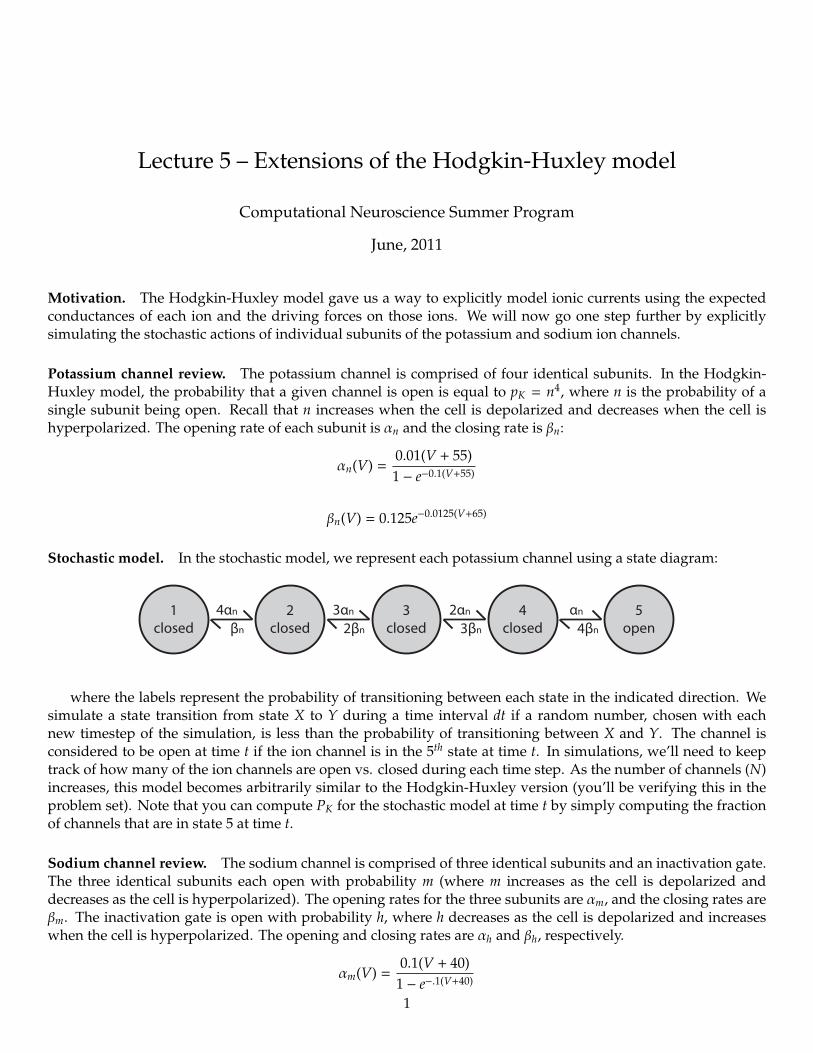
Stochastic model. In the stochastic model, we represent each potassium channel using a state diagram:

1closed

2closed

3closed

4closed

5open

4!n 3!n 2!n !n

"n 2"n 3"n 4"n

where the labels represent the probability of transitioning between each state in the indicated direction. Wesimulate a state transition from state X to Y during a time interval dt if a random number, chosen with eachnew timestep of the simulation, is less than the probability of transitioning between X and Y. The channel isconsidered to be open at time t if the ion channel is in the 5th state at time t. In simulations, we’ll need to keeptrack of how many of the ion channels are open vs. closed during each time step. As the number of channels (N)increases, this model becomes arbitrarily similar to the Hodgkin-Huxley version (you’ll be verifying this in theproblem set). Note that you can compute PK for the stochastic model at time t by simply computing the fractionof channels that are in state 5 at time t.

Sodium channel review. The sodium channel is comprised of three identical subunits and an inactivation gate.The three identical subunits each open with probability m (where m increases as the cell is depolarized anddecreases as the cell is hyperpolarized). The opening rates for the three subunits are αm, and the closing rates areβm. The inactivation gate is open with probability h, where h decreases as the cell is depolarized and increaseswhen the cell is hyperpolarized. The opening and closing rates are αh and βh, respectively.

αm(V) =0.1(V + 40)

1 − e−.1(V+40)

1

βm(V) = 4e−0.0556(V+65)

αh(V) = 0.07e−.05(V+65)

βn(V) =1

1 + e−.1(V+35)

Stochastic sodium channel model. In the Hodgkin-Huxley model, the three subunits and the inactivation gateare assumed to be independent (that’s why the probabilities are multiplied into m3h). However, this is not quitetrue. A more accurate description is something like the following:

1closed

2closed

3closed

4open

5inactivated

3αm 2αm αm k3βm 2βm 3βm

k1

k2αh

In particular, the ball mechanism of the inactivation gate is located inside the cell membrane, and cannot bedirectly affected by potential across the membrane. The inactivation gate only comes into play when at least oneof the subunits is open (i.e., when the channel occupies states 2, 3, or 4 in the diagram). In addition, according tothis model, if the neuron is in the inactivate state (state 5), it can only transition to state 3.

Whereas the transitions of the three subunits between states 1, 2, 3, and 4 in the stochastic model are identicalto in the Hodgkin-Huxley model, the behavior of the inactivation gate is much different – in particular, theinactivation gate in the stochastic model depends on the states of the three subunits.

As in the stochastic potassium channel model, you can compute the PNa for the stochastic sodium channel attime t by computing the fraction of sodium channels which occupy state 4 at that time.

Replacing the Hodgkin-Huxley channels with stochastic channels. In the Hodgkin-Huxley model, we com-puted PK = n4 and PNa = m3h with each time step, updating n,m, and h as we stepped through the model. In thestochastic model, we compute PK and PNa directly, so we no longer need to compute n, m, or h. Other than thedifference in computing PK and PNa, the stochastic model is identical to the Hodgkin-Huxley model.

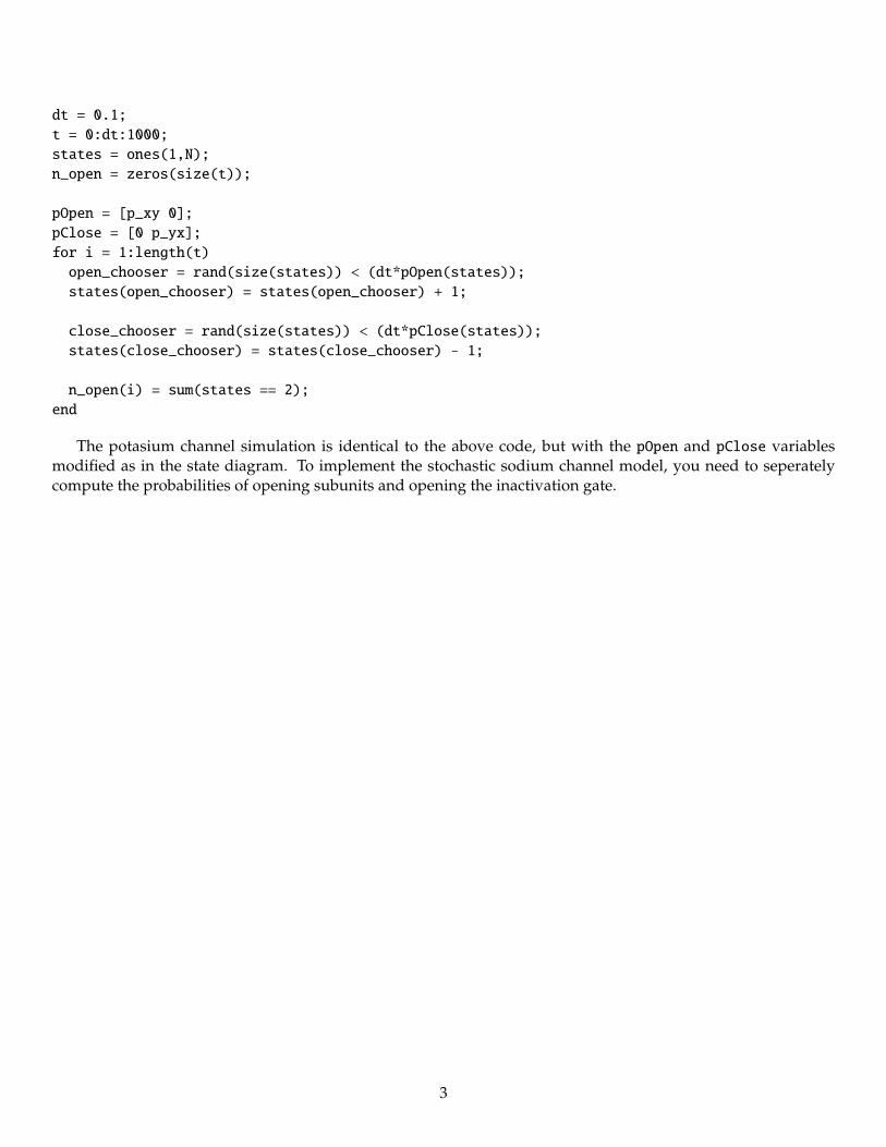
Some implementation suggestions. There are a number of possible ways to implement the stochastic channelmodels, with some methods being more efficient than others. Particularly when the number of channels is large,it becomes very important to code the simulation efficiently (read: vectorize!) if the simulation is to finish runningin a reasonable amount of time. To start you off, we’ll go through a simple two-state example. The states arex (closed) and y (open). Let’s suppose that the probability of transitioning from state x to state y is pxy and theprobability of transisitioning from y to x is pyx. To simulate N = 1000 of these simple two-state channels, we couldwrite something like the following:

2

dt = 0.1;

t = 0:dt:1000;

states = ones(1,N);

n_open = zeros(size(t));

pOpen = [p_xy 0];

pClose = [0 p_yx];

for i = 1:length(t)

open_chooser = rand(size(states)) < (dt*pOpen(states));

states(open_chooser) = states(open_chooser) + 1;

close_chooser = rand(size(states)) < (dt*pClose(states));

states(close_chooser) = states(close_chooser) - 1;

n_open(i) = sum(states == 2);

end

The potasium channel simulation is identical to the above code, but with the pOpen and pClose variablesmodified as in the state diagram. To implement the stochastic sodium channel model, you need to seperatelycompute the probabilities of opening subunits and opening the inactivation gate.

3

Problem Set 5 – Extensions of the Hodgkin-Huxley model

Computational Neuroscience Summer Program

June, 2011

In this problem set you will be extending the standard Hodgkin-Huxley model you constructed in ProblemSet 4. In this extended model we will be simulating the actions of individual voltage-dependent Sodium andPotassium channels. Feel free to re-use any code from Problem Set 4 that you think would be useful. Write upyour results in a text editor of your choosing. Include any relevant figures. Include a printout of your Matlabcode as well as any calculations that aren’t in the code. You may work individually or in groups, but each studentshould hand in their own report.

Equations

τx(V) dxdt = x∞(V) − x τx(V) = 1

αx(V)+βx(V) x∞(V) =αx(V)

αx(V)+βx(V)

αn(V) =.01(V+55)

1−exp(−.1(V+55)) αm(V) =0.1(V+40)

1−exp(−.1(V+40)) αh(V) = 0.07 ∗ exp(−.05(V + 65))βn(V) = 0.125 ∗ exp(−.0125(V + 65)) βm(V) = 4 ∗ exp(−.0556(V + 65)) βh(V) = 1

1+exp(−.1(V+35))PK = n4 PNa = m3hgK = gKPK gNa = gNaPNa

Problems

1. Construct and simulate the stochastic K+ channel model as shown in the state diagram below. The diagramshows transitions between different states of a K+ channel. The symbols αn and βn represent the opening andclosing rates, respectively, of individual K+ channels (these are the same variables you used in Problem Set 4).Set the rate constants equal to their value at 10 mV (i.e., use αn(10mV) = 0.65/ms and βn(10mV) = 0.05/ms).Transitions are made between states with each iteration of your program if a random number chosen uniformlybetween 0 and 1 is less than the corresponding rate for that transition time. For example, if a channel is in state 1,that channel will transition to state 2 during the current iteration of your program if the chosen random numberis less than 4αndt. As the channel(s) make transitions between states, keep track of whether state 5 is occupied. Ifso, assume that each channel conducts 1 pA (10−12 A) of current; otherwise no current flows through the channel.Plot currents generated by this model for N =1, 10, and 100 channels over a 20 ms period (use dt = 0.01 ms).

1closed

2closed

3closed

4closed

5open

4!n 3!n 2!n !n

"n 2"n 3"n 4"n

2. The Hodgkin-Huxley description of the K+ channel predicts the current flowing in these simulations wouldbe Nn4 pA, where N is the number of K+ channels and n is the K+ activation variable (same as in Problem Set4). On a single plot, show the amount of current predicted by the Hodgkin-Huxley prediction and the amount ofcurrent predicted with the stochastic model. (Use N = 1000.)

1

3. Construct an stochastic Na+ channel model analogous to the K+ model, using the state diagram below. Thesymbols αm and βm represent opening and closing rates of the three main subunits of the sodium channel. Acti-vation and deinactivation rates of the sodium channel gate are represented by k1, k2, and k3. Set the rate constantsequal to their value at 10 mV (i.e., use αm(10 mV) =5.034/ms, αh(10 mV) =0.0016/ms, and βm(10 mV) =0.0618/ms).Use k1 = 0.24/ms, k2 = 0.4/ms, and k3 = 1.5/ms. As the channel(s) make transitions between states, keep track ofwhether state 4 is occupied. If so, assume that each channel conducts -1 pA (10−12 A) of current; otherwise nocurrent flows through the channel. Plot currents generated by this model for M =1, 10, and 100 channels over a20 ms period.

1closed

2closed

3closed

4open

5inactivated

3αm 2αm αm k3βm 2βm 3βm

k1

k2αh

4. The Hodgkin-Huxley description of the Na+ channel predicts the current flowing in these simulations wouldbe Mm3h pA, where M is the number of Sodium channels. On a single plot, show the amount of currentpredicted by the Hodgkin-Huxley prediction and the amount of current predicted with the stochastic model.(Use M = 1000.)

5. Challenge problem. Modify the Hodgkin-Huxley model from Problem Set 5 to explicitly simulate Sodiumand Potassium channels using the stochastic models above (to start, use N = M = 1000). You will need toupdate the transition probabilities αn, αm, αh, βn, and βm with each time step, since those transition probabilitiesare voltage-dependent. k1, k2, and k3 are constants. Hint: PX is equal to the total proportion of X channelscurrently open. Simulate a 20 ms interval. Apply an external current of Iext = 5 nA/mm2 from 5 to 8 ms. Plot V,PK, and PNa as a function of time.

2

Computing a spike-triggered average

Two-spike-triggered average

• You might expect that the two-spike average would be a linear summation of the single-spike averages.

• However, at some neurons multiple spikes are caused by especially large input signals.

Problem Set 6 -- Introduction to data analysis

Computational Neuroscience Summer Program

June, 2011

These questions use two Matlab files:! http://www.neurotheory.columbia.edu/~larry/book/exercises/c1/data/c1p8.mat

! http://www.neurotheory.columbia.edu/~larry/book/exercises/c1/data/c2p3.mat

These questions were adapted from Dayan & Abbott, who in turn took inspiration from Sebastian Seung.

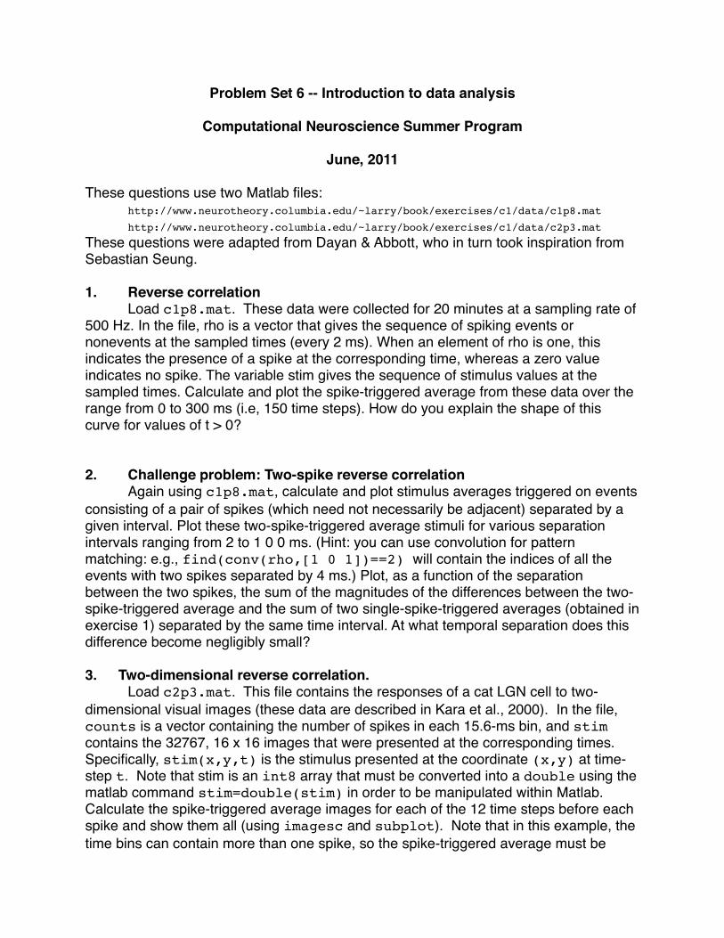
1.! Reverse correlation! Load c1p8.mat. These data were collected for 20 minutes at a sampling rate of 500 Hz. In the file, rho is a vector that gives the sequence of spiking events or nonevents at the sampled times (every 2 ms). When an element of rho is one, this indicates the presence of a spike at the corresponding time, whereas a zero value indicates no spike. The variable stim gives the sequence of stimulus values at the sampled times. Calculate and plot the spike-triggered average from these data over the range from 0 to 300 ms (i.e, 150 time steps). How do you explain the shape of this curve for values of t > 0?

2.! Challenge problem: Two-spike reverse correlation! Again using c1p8.mat, calculate and plot stimulus averages triggered on events consisting of a pair of spikes (which need not necessarily be adjacent) separated by a given interval. Plot these two-spike-triggered average stimuli for various separation intervals ranging from 2 to 1 0 0 ms. (Hint: you can use convolution for pattern matching: e.g., find(conv(rho,[1 0 1])==2) will contain the indices of all the events with two spikes separated by 4 ms.) Plot, as a function of the separation between the two spikes, the sum of the magnitudes of the differences between the two-spike-triggered average and the sum of two single-spike-triggered averages (obtained in exercise 1) separated by the same time interval. At what temporal separation does this difference become negligibly small?

3. Two-dimensional reverse correlation.! Load c2p3.mat. This file contains the responses of a cat LGN cell to two-dimensional visual images (these data are described in Kara et al., 2000). In the file, counts is a vector containing the number of spikes in each 15.6-ms bin, and stim contains the 32767, 16 x 16 images that were presented at the corresponding times. Specifically, stim(x,y,t) is the stimulus presented at the coordinate (x,y) at time-step t. Note that stim is an int8 array that must be converted into a double using the matlab command stim=double(stim) in order to be manipulated within Matlab. Calculate the spike-triggered average images for each of the 12 time steps before each spike and show them all (using imagesc and subplot). Note that in this example, the time bins can contain more than one spike, so the spike-triggered average must be

computed by weighting each stimulus by the number of spikes in the corresponding time bin, rather than weighting it by either 1 or 0 depending on whether a spike is present or not. (Tip: Make the plots look even cleaner by using the same color scale limits for all plots (search ʻclimʼ).) In the averaged images, you should see a central receptive field that reverses sign over time. Also, by summing up the images across one spatial dimension, produce a figure like the one below that plots the response as a function of time (τ) and one spatial dimension (x).