Chapter 6 : exchange rate determination : theory Finance/ch6/chap6.pdfsome variation in the value of the currency (depreciation of the currency) and they intervene when the exchange

Chapter 6 : exchange ratedetermination : theory

Michel BEINE

Chapter 6 : exchange rate determination : theory – p. 1/31

Section 1 : introduction


Introduction

In this chapter, look at theoretical approachesexplaining the behaviour of exchange rates → Useful to

Understand the macroeconomic conditions affectingexchange rates → allows to estimate the fundamentalvalue of the exchange rate.

Take corrective actions in terms of policy

Predict exchange rates


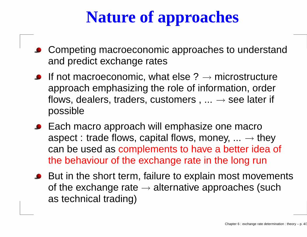
Nature of approaches

Competing macroeconomic approaches to understandand predict exchange rates

If not macroeconomic, what else ? → microstructureapproach emphasizing the role of information, orderflows, dealers, traders, customers , ... → see later ifpossible

Each macro approach will emphasize one macroaspect : trade flows, capital flows, money, ... → theycan be used as complements to have a better idea ofthe behaviour of the exchange rate in the long run

But in the short term, failure to explain most movementsof the exchange rate → alternative approaches (suchas technical trading)


Macro approaches

The trade elasticity approach

The PPP approach with Balassa-Samuelson dimension

The monetary view of the exchange rate determinantion

The portfolio balance approach


Section 2 : The Elasticity View of the exchange rate


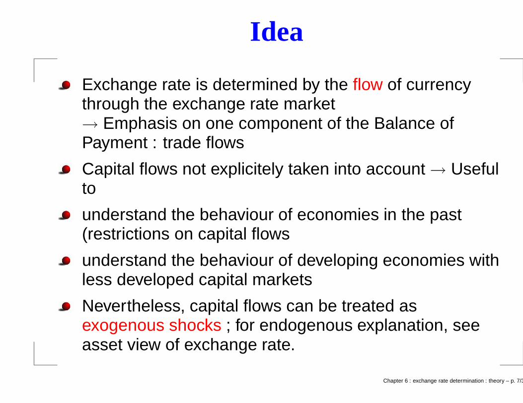
Idea

Exchange rate is determined by the flow of currencythrough the exchange rate market→ Emphasis on one component of the Balance ofPayment : trade flows

Capital flows not explicitely taken into account → Usefulto

understand the behaviour of economies in the past(restrictions on capital flows

understand the behaviour of developing economies withless developed capital markets

Nevertheless, capital flows can be treated asexogenous shocks ; for endogenous explanation, seeasset view of exchange rate.


Comments on Figure

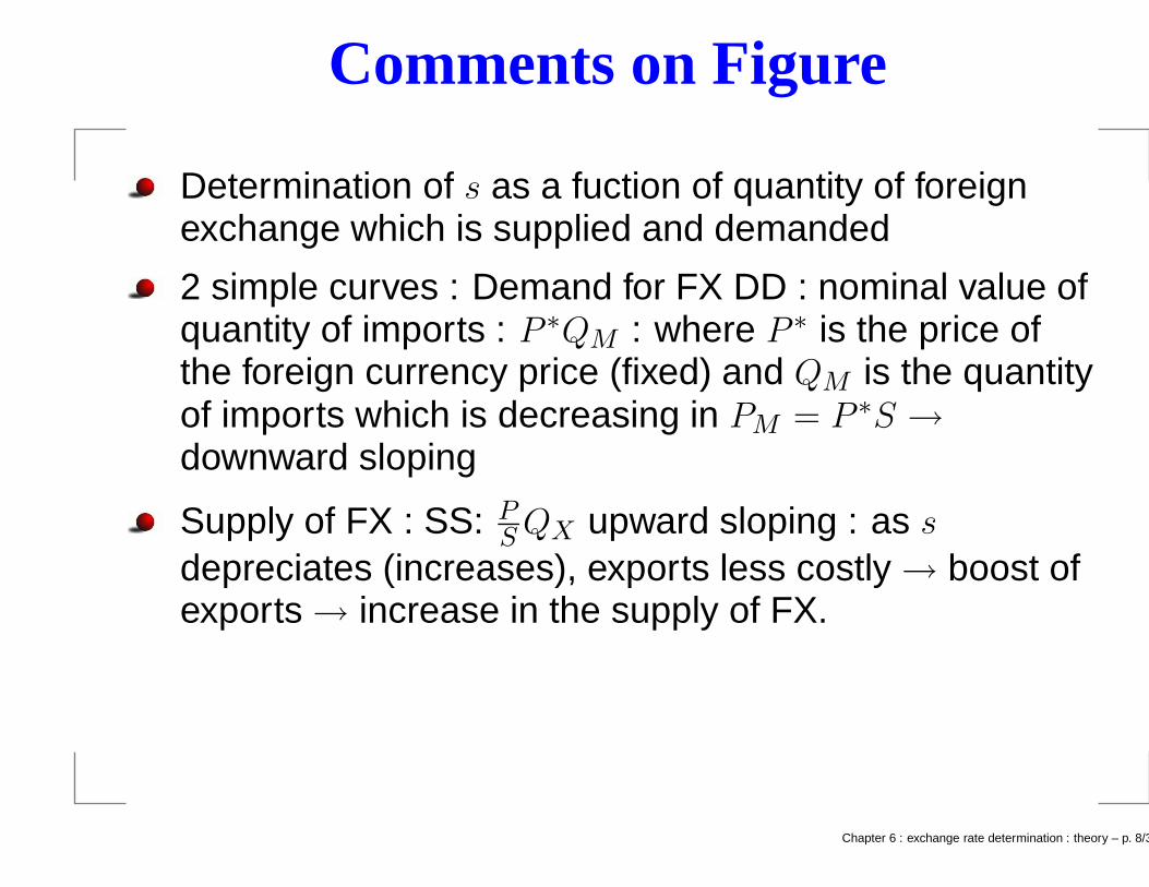
Determination of s as a fuction of quantity of foreignexchange which is supplied and demanded

2 simple curves : Demand for FX DD : nominal value ofquantity of imports : P ∗QM : where P ∗ is the price ofthe foreign currency price (fixed) and QM is the quantityof imports which is decreasing in PM = P ∗S →downward sloping

Supply of FX : SS: PSQX upward sloping : as s

depreciates (increases), exports less costly → boost ofexports → increase in the supply of FX.


Pegging the exchange rate

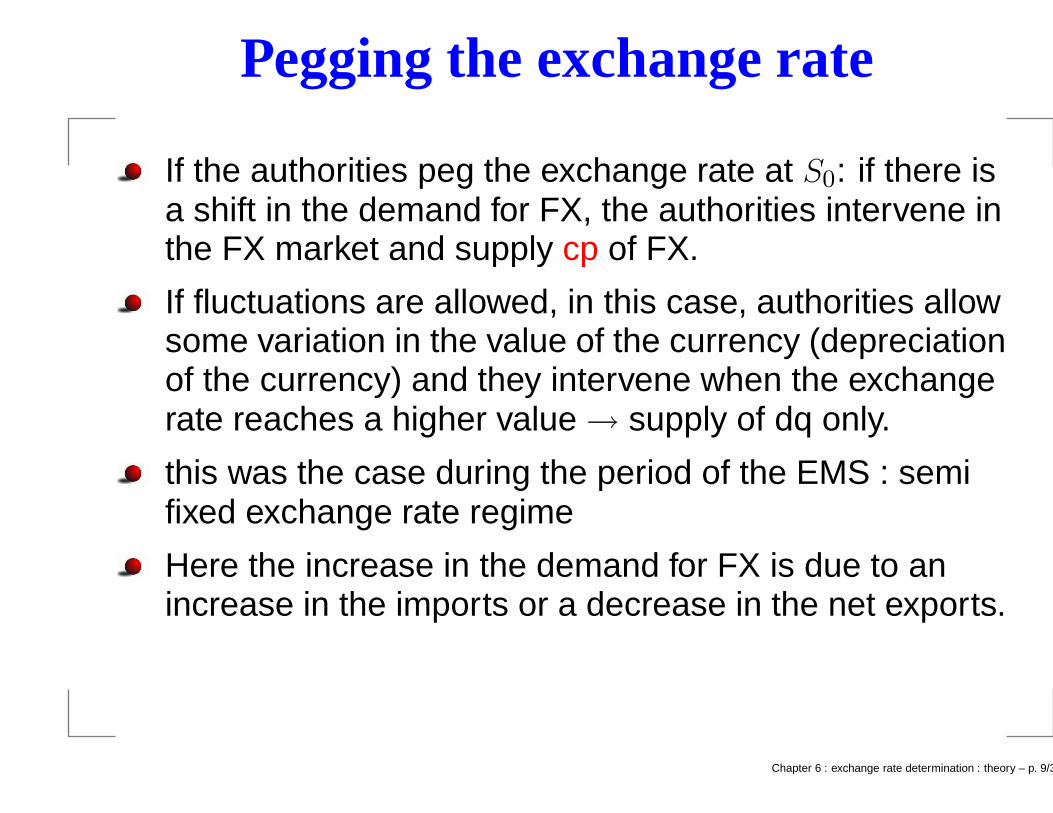
If the authorities peg the exchange rate at S0: if there isa shift in the demand for FX, the authorities intervene inthe FX market and supply cp of FX.

If fluctuations are allowed, in this case, authorities allowsome variation in the value of the currency (depreciationof the currency) and they intervene when the exchangerate reaches a higher value → supply of dq only.

this was the case during the period of the EMS : semifixed exchange rate regime

Here the increase in the demand for FX is due to anincrease in the imports or a decrease in the net exports.


The Marshall-Lerner condition

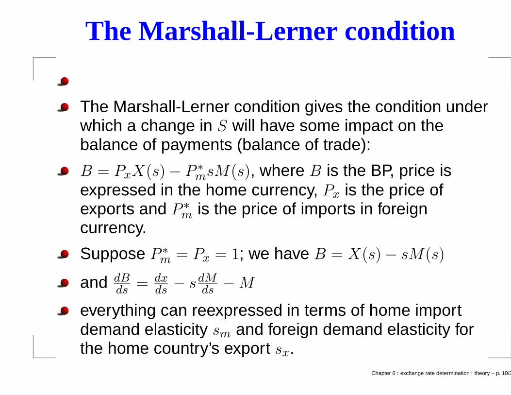
The Marshall-Lerner condition gives the condition underwhich a change in S will have some impact on thebalance of payments (balance of trade):

B = PxX(s) − P ∗

msM(s), where B is the BP, price isexpressed in the home currency, Px is the price ofexports and P ∗

m is the price of imports in foreigncurrency.

Suppose P ∗

m = Px = 1; we have B = X(s) − sM(s)

and dBds

= dxds

− sdMds

− M

everything can reexpressed in terms of home importdemand elasticity sm and foreign demand elasticity forthe home country’s export sx.



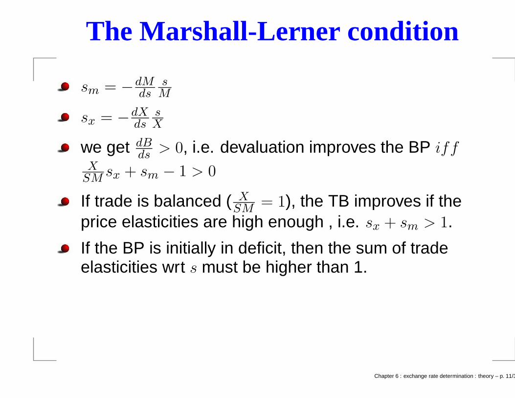
sm = −dMds

sM

sx = −dXds

sX

we get dBds

> 0, i.e. devaluation improves the BP iffX

SMsx + sm − 1 > 0

If trade is balanced ( XSM

= 1), the TB improves if theprice elasticities are high enough , i.e. sx + sm > 1.

If the BP is initially in deficit, then the sum of tradeelasticities wrt s must be higher than 1.



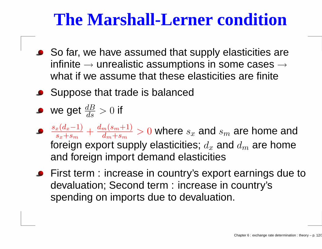
So far, we have assumed that supply elasticities areinfinite → unrealistic assumptions in some cases →what if we assume that these elasticities are finite

Suppose that trade is balanced

we get dBds

> 0 if

sx(dx−1)sx+sm

+ dm(sm+1)dm+sm

> 0 where sx and sm are home andforeign export supply elasticities; dx and dm are homeand foreign import demand elasticities

First term : increase in country’s export earnings due todevaluation; Second term : increase in country’sspending on imports due to devaluation.


Impact of devaluation on B

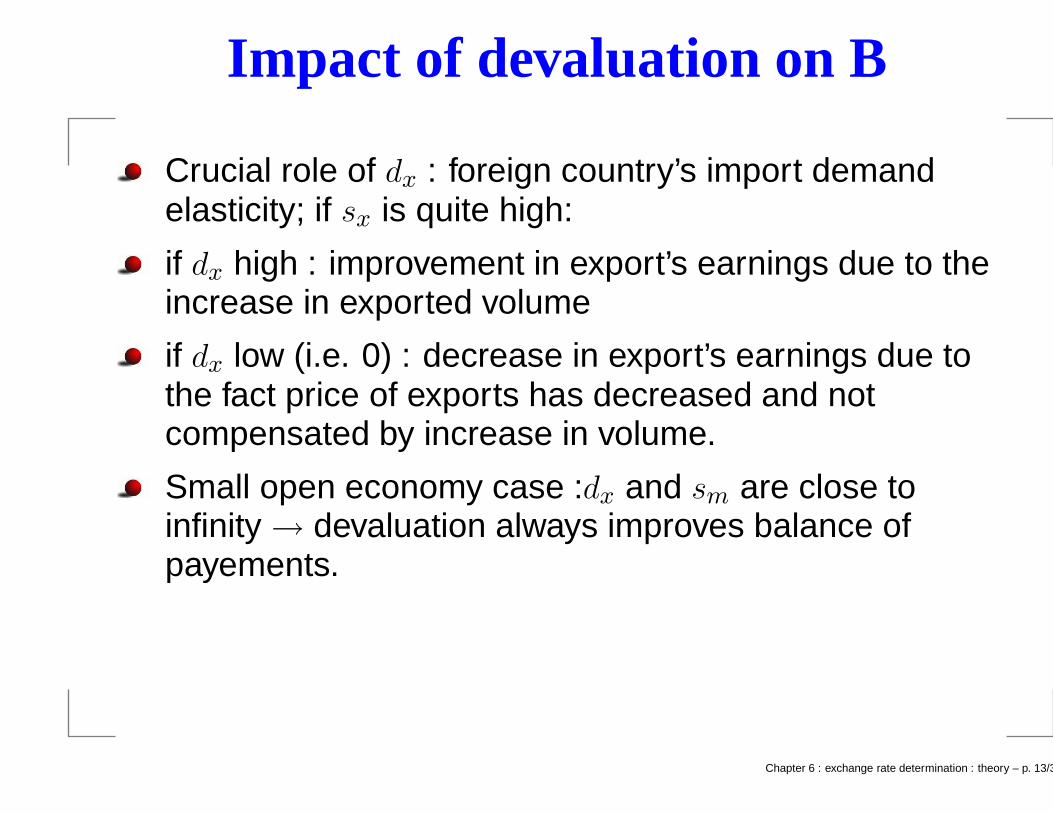
Crucial role of dx : foreign country’s import demandelasticity; if sx is quite high:

if dx high : improvement in export’s earnings due to theincrease in exported volume

if dx low (i.e. 0) : decrease in export’s earnings due tothe fact price of exports has decreased and notcompensated by increase in volume.

Small open economy case :dx and sm are close toinfinity → devaluation always improves balance ofpayements.


cases ofdx

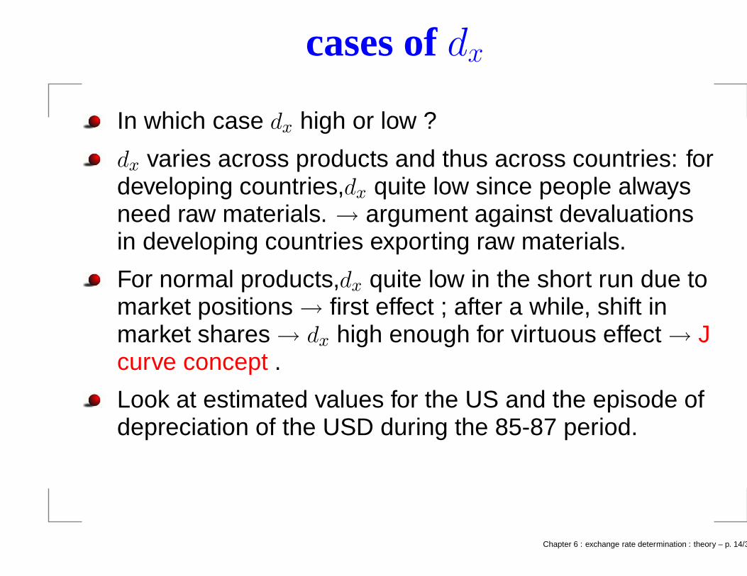
In which case dx high or low ?

dx varies across products and thus across countries: fordeveloping countries,dx quite low since people alwaysneed raw materials. → argument against devaluationsin developing countries exporting raw materials.

For normal products,dx quite low in the short run due tomarket positions → first effect ; after a while, shift inmarket shares → dx high enough for virtuous effect → Jcurve concept .

Look at estimated values for the US and the episode ofdepreciation of the USD during the 85-87 period.


US case

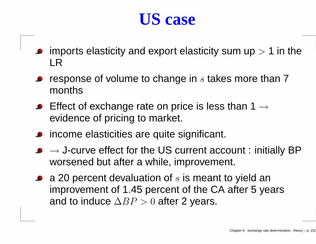
imports elasticity and export elasticity sum up > 1 in theLR

response of volume to change in s takes more than 7months

Effect of exchange rate on price is less than 1 →evidence of pricing to market.

income elasticities are quite significant.

→ J-curve effect for the US current account : initially BPworsened but after a while, improvement.

a 20 percent devaluation of s is meant to yield animprovement of 1.45 percent of the CA after 5 yearsand to induce ∆BP > 0 after 2 years.


Section 3 : The Monetary View of Exchange RateDetermination


2 approaches

The flexible price approach assumes that prices areflexible;

In contrast, sticky price approach assumes that pricesare fixed in the short run → long run identical whileshort run different

the sticky price model gives rise to the famousovershooting properties of the exchange rate

In the flex-price approach, PPP is assumed to hold →not supported empirically → might explain whypredictions using the FLMA are not very good.


The flex-price approach

Idea : theory of price determination along with PPP

We consider here a 2-country version : variables with *refer to foreign variables

Each country produces a good and goods are perfectsubstitutes; PPP is assumed to hold :st = pt − p∗t (everything is in log)

In the flex-price approach, PPP is assumed to hold →not supported empirically → might explain why not sogood predictions.

Capital is perfectly mobile and asset holders canrebalance their portfolio instantly


The flex-price approach

Equilibrium in the money markets: △set+1 = (i − i∗)t

Wealth constraint for domestic resident (counterpart forforeign residents not written here) : W = M + B + B∗ orW = M + V where M denotes stock of money and Brefer to bonds. Bonds are perfect substitutes.

equilibrium in the money market implies equilibrium inthe bond markets and the other way around. → focuson the money market → this is why one calls monetaryapproach.

Money demand relationships (Cagan demand formoney): mD

t − pt = α1yt − α2it andmD∗

t − p∗t = α1y∗

t − α2i∗

t

Equilibria in both money markets: mDt = ms

t = mt andmD∗

t = ms∗t = m∗

t Chapter 6 : exchange rate determination : theory – p. 19/31

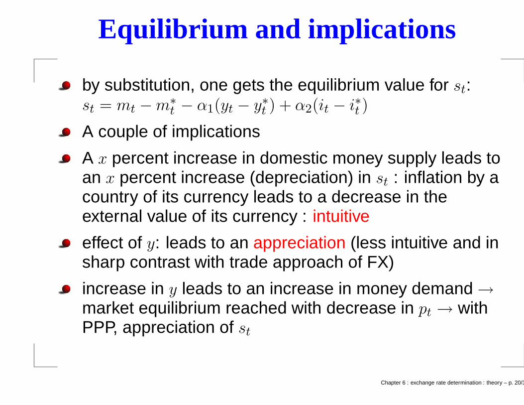
Equilibrium and implications

by substitution, one gets the equilibrium value for st:st = mt − m∗

t − α1(yt − y∗t ) + α2(it − i∗t )

A couple of implications

A x percent increase in domestic money supply leads toan x percent increase (depreciation) in st : inflation by acountry of its currency leads to a decrease in theexternal value of its currency : intuitive

effect of y: leads to an appreciation (less intuitive and insharp contrast with trade approach of FX)

increase in y leads to an increase in money demand →market equilibrium reached with decrease in pt → withPPP, appreciation of st


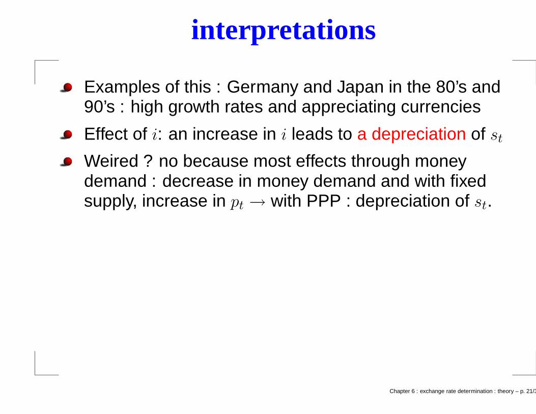
interpretations

Examples of this : Germany and Japan in the 80’s and90’s : high growth rates and appreciating currencies

Effect of i: an increase in i leads to a depreciation of st

Weired ? no because most effects through moneydemand : decrease in money demand and with fixedsupply, increase in pt → with PPP : depreciation of st.


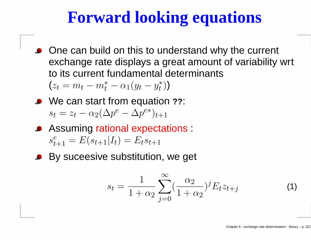
Forward looking equations

One can build on this to understand why the currentexchange rate displays a great amount of variability wrtto its current fundamental determinants(zt = mt − m∗

t − α1(yt − y∗t ))

We can start from equation ??:st = zt − α2(∆pe − ∆pe∗)t+1

Assuming rational expectations :set+1 = E(st+1|It) = Etst+1

By suceesive substitution, we get

st =1

1 + α2

∞∑

j=0

(α2

1 + α2)jEtzt+j (1)


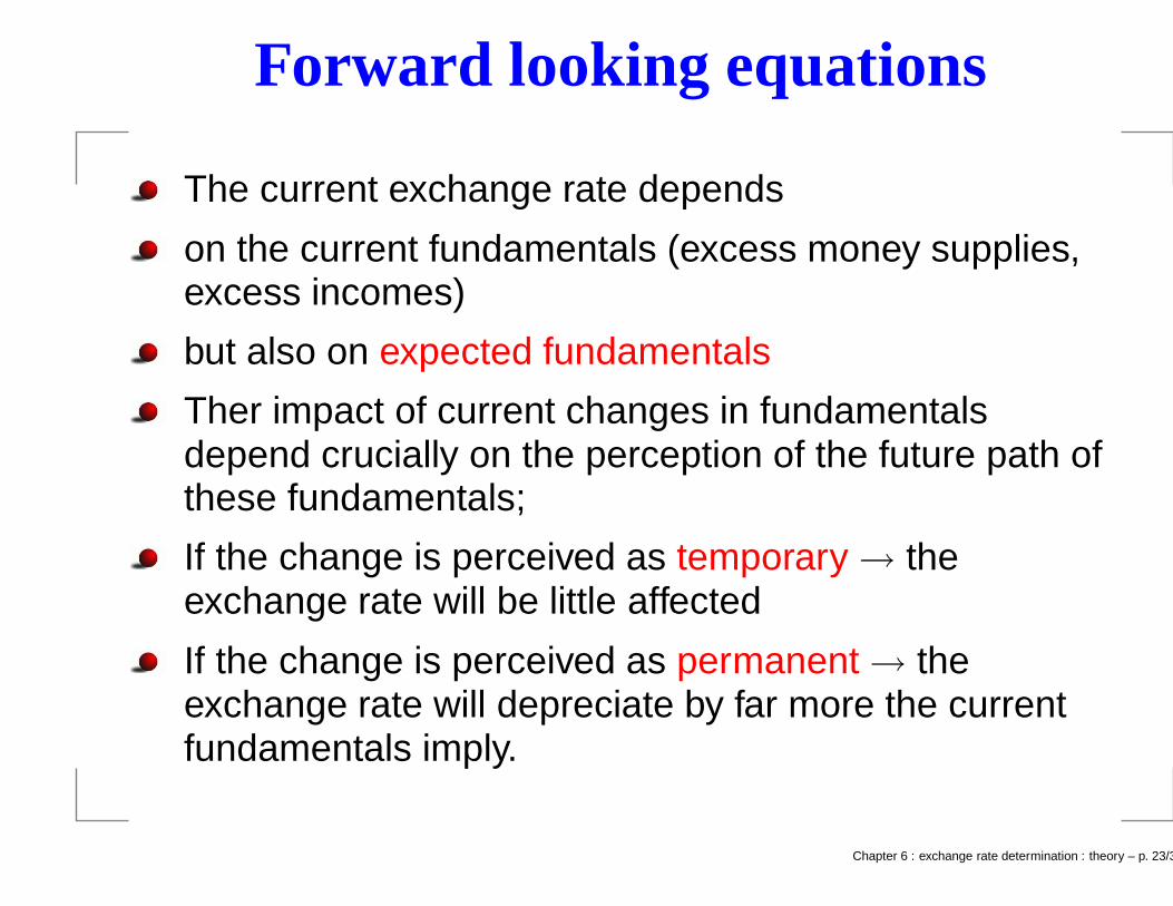
Forward looking equations

The current exchange rate depends

on the current fundamentals (excess money supplies,excess incomes)

but also on expected fundamentals

Ther impact of current changes in fundamentalsdepend crucially on the perception of the future path ofthese fundamentals;

If the change is perceived as temporary → theexchange rate will be little affected

If the change is perceived as permanent → theexchange rate will depreciate by far more the currentfundamentals imply.


The sticky price version

The monetary approach also has a sticky price version

pt is sticky in the short-run but not in the long run →PPP holds in the LR but not in the short run

This induces some overshooting properties of st: theexchange rate depreciates by more than implied in thelong run by the change in the fundamentals (e.g.excessive money supply).


Mecanisms in the sticky price version

Basic mecanisms.

prices are sticky in the SR, flex in the LR

money demand depends on domestic prices (+) anddomestic interest rates (-)

Uncovered interest rate parity holds on a continuousbasis : it − i∗t = △se

t+1

suppose unexpected increase in domestic moneysupply

to restore the equilibrium, either increase in domesticprices or-and decrease in domestic interest rates


Mecanisms in the sticky price version

But if prices are sticky, decrease in i below i∗ requires△se

t+1 > 0

for this to be possible, one needs that agents anticipe afuture exchange rate appreciation → overshooting of swrt to the long run value.

analysis in terms of figures.


Section 3 : The Portfolio view of Exchange RateDetermination


Weaknesses of previous analysis

Big weakness of previous approach

No role for stock variables

No role for a role of a change in asset stocks →approach accounting for change in positions in assetpositions.


Idea of portfolio approach

Circular determination

Asset stocks

Changes lead to changes in asset prices : interest rates(bonds and money) and exchange rates (currency)

Change leads in changes in in real wealth and realexchange rates

This will affect the current account → changes in netforeign assets

This leads to a change in stocks of assets .


The portfolio approach

No clear evidence in favour of this approach

Nevertheless, might explain some episodes ofexchange rate dynamics that cannot be explained bythe monetary approach

Example : 1978-79 period : Monetary growth inGermany in excess of US monetary growth and ofGerman income growth → the monetary approachwould predict Dmark depreciation

Observe Dmark appreciation wrt USD. Why ? Germancurrent account surplus and US current account deficit→ increase in demand for German assets.


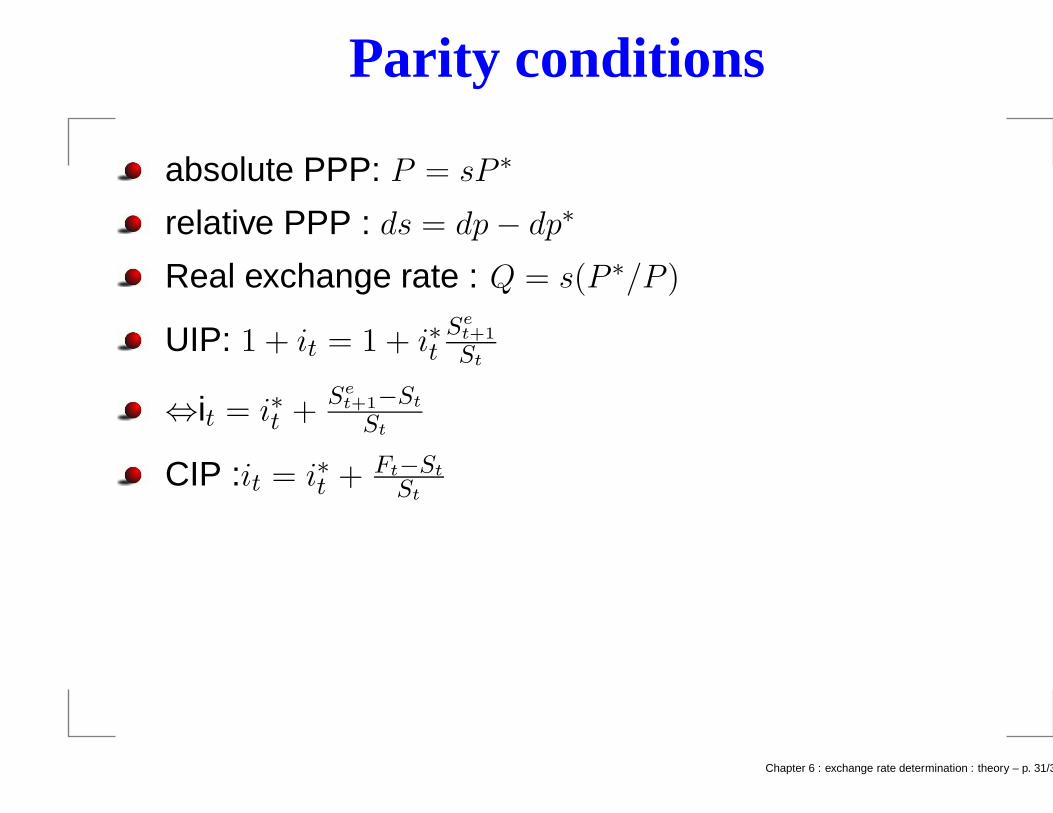
Parity conditions

absolute PPP: P = sP ∗

relative PPP : ds = dp − dp∗

Real exchange rate : Q = s(P ∗/P )

UIP: 1 + it = 1 + i∗tSe

t+1

St

⇔it = i∗t +Se

t+1−St

St

CIP :it = i∗t + Ft−St

St


Documents

Chapter 6 : exchange rate determination : theory Finance/ch6/chap6.pdfsome variation in the value of the currency (depreciation of the currency) and they intervene when the exchange