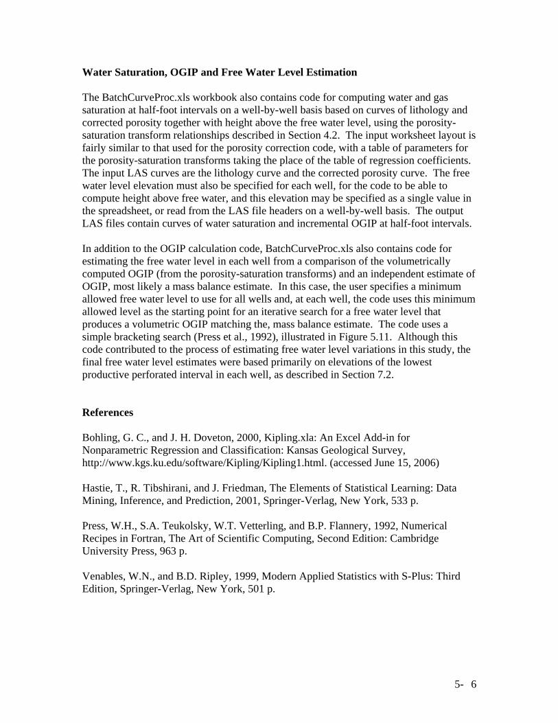
CHAPTER 5. TECHNOLOGY TO MANAGE LARGE DIGITAL DATASETS Geoffrey C. Bohling Introduction Development of the Hugoton field model has required automated processing of large data volumes at several steps, including prediction of lithofacies from geophysical well logs in numerous wells based on a neural network trained on log-facies associations observed in cored wells, generation of geologic controlling variables (depositional environment indicator and relative position in cycle) from a tops dataset, and computation of porosities corrected for mineralogical variations between facies and for washouts. In addition, we have developed code for batch processing the predicted facies and corrected porosities at the wells to estimate water saturations and original gas in place using petrophysical transforms and height above free-water level, providing a quickly computed measure of the plausibility of the geomodel. This chapter describes the data management and facies-prediction tools developed for this project, which we have provided in the form of two Excel workbooks and an Excel add-in. Having automation tools allowed us to efficiently handle large volumes of data and the ability to perform the multiple iterations required to test preliminary and intermediate algorithms and solutions. Facies-prediction Tools Prediction of facies from wire-line logs in 1600 “node” wells distributed throughout the field was a critical step in developing the Hugoton field model. The primary tool used in this process was a single hidden layer network (Hastie et al., 2001) designed for prediction of a categorical output variable (facies) from a set of continuous input variables (logs), as illustrated in Figure 5.1. We have implemented the neural network in Excel, adding the neural network training and prediction code to a previously existing Excel add-in for nonparametric regression and classification, Kipling.xla (Bohling and Doveton, 2000). The new version of the add-in, Kipling2.xla, includes code for batch prediction of facies (or of any other categorical or continuous variable) based on logs read from a set of LAS files, with prediction results being written out as curves in a corresponding set of output LAS files. The computationally intensive task of determining the optimal neural network parameters based on crossvalidation of the training dataset, from wells with both core and log data, was performed outside Excel, using scripts written in the R statistical language. Prior to performing facies prediction, we added two geologic constraining variables to the set of log values: a code representing the depositional environment (1 - nonmarine, 2 - marine, or 3 - intertidal) associated with each of the 25 members (half-cycles) in the model, and a curve representing the relative vertical position within each half-cycle, ranging from 0 at the base to 1 at the top. The depositional environment indicator variable, MnM, helps to distinguish between lithofacies with similar petrophysical

5- 1

properties but developed in different broad depositional environments. Including the relative position curve, RelPos, allowed the network to encode information regarding the fairly regular succession of lithofacies succession commonly exhibited within each interval, and thus transfer some of that character to the sequence of predicted lithofacies in each well. The two curves were computed from a database of formation tops using Visual Basic code within an Excel spreadsheet. They were then combined with the wire-line log curves to complete the feature vector used as input to the neural network.

Depositional Environment Code and Relative Position Curve The depositional environment code (MnM) and relative position (RelPos) curves are generated by Visual Basic code in an Excel workbook named GenMnM.xls. Figure 5.2 shows the layout of an input spreadsheet for the workbook. The fundamental input information is a set of formation names or labels, listed in order of increasing depth in row 5, and a set of top depths for each formation by well, with wells identified by API number (or some other unique identifier) in column A, starting from row 9, and top depths for each well listed to the right of the API number, each in the appropriate column for the formation. The data shown in Figure 5.2 have been extracted from the Kansas Geological Survey’s database of Hugoton top depths, imported into Excel from Oracle. However, the code is completely general and will work with any set of tops. The spreadsheet in Figure 5.2 contains additional columns of data to the right of those shown in the figure, with tops continuing down through the Council Grove. The code will generate a set of LAS files containing the two geologic constraining variables, and cell B2 on the spreadsheet contains the name of the folder to which these files should be written. Cell B3 specifies the depth increment (here 0.5 feet) at which the curves should be written. Row 6 contains the depositional environment code numbers associated with each formation. The numbers shown here are those appropriate for the current study, but any set of code numbers could be employed. Row 7 contains a list of “default” thicknesses for each formation. The default thicknesses come into play when there is a gap in the tops sequence for a well. In this case, information for the last formation above the gap is written out on the basis of the default thickness for that formation, with null values being written out below the depth given by the top depth plus the default thickness (unless the next top depth below the gap is encountered first). Once the input information is set up on the spreadsheet, clicking on the Generate MnM Files button will launch the Visual Basic code, generating a set of output LAS files in the specified output folder. This folder should be created in advance of running the code, using Windows Explorer. Each output file is named MnMnnnn.las, where nnnn is replaced by the API number listed in the spreadsheet. Figure 5.3 shows the headers and first few data lines of the LAS file generated from the first line of data shown in Figure 5.2.

5- 2

Neural Network Prediction of Lithofacies As discussed in Chapter 6, we explored several approaches for predicting lithofacies from logs and ended up choosing to use a neural network. The neural network implemented in Kipling2.xla is a simple single hidden-layer feed-forward network, as illustrated in Figure 5.1 and described in Chapter 11 of Hastie et al. (2001). Each hidden layer node in the network computes a linear combination or weighted sum of the input variables (logs), representing variation along a certain direction in the input variable space. The lines connecting the input and hidden layer nodes represent the weights in this linear combination. This weighted sum is then passed through a sigmoid transfer function, with output values ranging between zero and one, forming an S-shaped basis function along the direction represented by the linear combination. Each output layer node then computes a linear combination of the sigmoid basis function values computed by the hidden layer nodes and the entire set of linear combinations computed by the output nodes is rescaled to represent a set of probabilities of facies membership. Thus, on a single forward pass, the network transforms a set of log values into an associated set of probabilities of facies occurrence. The network is trained based on a set of training data where both log values and facies are known, in this case data from the 28 cores described in the field. In the training process, the network weights are iteratively adjusted until the set of facies predicted by the network match the set of core facies as closely as possible. However, the training process starts from a random set of initial weights and will generally converge to a different set of final weights for a different set of initial weights, meaning that there can be multiple, equally likely “realizations” of the trained neural network based on a single training dataset. The primary parameters controlling the behavior of the neural network are the number of hidden layer nodes and a damping or decay parameter. Increasing the number of hidden layer nodes allows the network to more closely reproduce the details of the training dataset, while fewer hidden layer nodes results in more generalized representation of the training data. Increasing the damping parameter forces the network weights to be smaller in magnitude, which results in a smoother or more generalized representation of the training data. Using a very large number of hidden-layer nodes and no or very little damping would allow the network to reproduce the training dataset very accurately, but this would almost certainly result in reduced accuracy in predictions on other datasets, a situation referred to as overtraining. Thus, the number of hidden-layer nodes (network size) and damping parameter should be adjusted to produce the optimal balance between detail and generalization. This optimization is usually achieved through crossvalidation, holding out different portions of the full training dataset from the training process, predicting on the withheld data and comparing predicted and true facies, and repeating the process many times over in order to obtain representative summaries of the prediction behavior for different parameter combinations. This process is much too computationally intensive to perform in Excel, so for this study we have used R language scripts to perform the crossvalidation, using R’s nnet function (Venables and Ripley, 1999), which

5- 3

implements the same style of neural network as in Kipling2.xla. The details and results of the crossvalidation process for this study are described in Chapter 6. For training a neural network in Kipling2.xla, the training data, including logs and known facies values from a set of wells, must be gathered together in one Excel spreadsheet, with logs and facies values, coded as a set of integers, in columns and data points – that is, the set of data for each measurement depth in each well – in rows, with a row of column labels at the top. Figure 5.4 shows the dialog box for selecting the predictor variables (logs) and categorical response variable (the variable L10, representing facies codes) from a training data worksheet. The user has also entered a comment which will be transferred to the output neural network worksheet as a reminder of what the worksheet represents. Figure 5.5 shows the dialog box for specifying the neural network parameters to use in the training process. In addition to the number of hidden-layer nodes (network size) and damping parameter, the user can also specify the number of iterations in the training process. More iterations will allow a closer reproduction of the training data. We have generally left the number of iterations at 100, controlling the network behavior through the network size and damping parameter. The values of these two parameters shown in Figure 5.5, 20 and 1.0, were the optimal values determined by the crossvalidation process described in Chapter 6 (in most cases). Once the training process starts, the code will generate a new worksheet and starting writing out the value of the objective function, a measure of the discrepancy between predicted and actual facies values over the entire training dataset, versus iteration number. The objective function will decrease with each iteration, more rapidly at first and gradually leveling off, indicating a point of diminishing return in further adjustments of the network weights. After the training process has completed, the user may use standard Excel plotting functions to generate a plot of objective function versus iteration number, as shown in Figure 5.6. After training is completed, the new worksheet will be populated with a set of numbers representing the weights in the trained neural network, along with summary statistics for the predictor variables (logs) in the training dataset. These numbers are not really intended for human consumption; they just need to be stored somewhere so that they can be used for prediction. The trained network can then be used for predicting facies from log values stored in an Excel worksheet, with results being written to a new worksheet, or predicting facies in batch based on logs in a set of LAS files, with results being written out to a new set of LAS files. For the batch-prediction process, the user needs to specify the correspondence between the logs used in the training process – the model variables – and the logs included in the LAS files. The batch-prediction code first presents the user with a standard dialog box for opening a file, asking the user to navigate to the folder containing the LAS files and open one of these files. The set of log mnemonics listed in the curve information section in this file is assumed to represent the set of mnemonics for the entire set of files, at least for the logs used in the prediction process. In other words, aliasing of logs to a common set of mnemonics has to have been done in advance. Figure 5.7 shows the dialog box for

5- 4

matching LAS file log mnemonics (Logs in file) to the log names used in the training process and stored in the neural network worksheet (Model variables). Figure 5.8 shows a portion of an output LAS file produced by the batch prediction process, including the curve information section of the headers and a few of the output data lines. The output curves include the predicted facies code at each depth, here labeled PredLL8, the probability of occurrence of each facies at each depth, here labeled ProbPE1 – ProbPE8. The predicted facies code is that associated with the largest occurrence probability. This batch-prediction process has been critical to the development of the Hugoton field model, allowing rapid production of facies curves from a large number of input LAS files. Porosity Correction The porosity correction code performs two tasks, first compensating for variations from the reference mineralogy for the neutron and density porosity logs and then applying an ad-hoc process to correct for washouts. The compensation for mineralogical variations employs the lithofacies-specific regression relationships between core and log porosity measurements described in Section 4.3. The correction for washouts removes porosity spikes identified as washouts on the basis of lithofacies-specific threshold values of the neutron-density crossplot porosity, and also levels out the “shoulders” leading up to these spikes, as illustrated in Figure 5.9. The user specifies both the threshold crossplot porosity value used to identify washouts and a replacement porosity value to use as the corrected porosity over the region identified as washout plus the shoulders leading up to the peak, typically an expected mean porosity value for the lithology. Note that Figure 5.9 is a little deceiving in that it treats the crossplot and corrected porosity curves as if they were one and the same; in reality, the washout-and-shoulder identification is done on the basis of the crossplot porosity, but the substitution is performed on the corrected porosity curve. The porosity-correction code is contained in a workbook named BatchCurveProc.xls, which is included in the appendix, along with documentation. This workbook also contains the code for batch computation of original gas in place and estimation of free water level, described in the next section. In the input worksheet for porosity correction, illustrated in Figure 5.10, the user specifies the folder containing the input LAS files and the names of the lithology, neutron porosity, density porosity, and crossplot porosity curves in those files, along with the name of an output folder to contain the LAS files with corrected porosity curves. The table to the right contains the set of coefficients for the regressions of core porosity versus neutron and density porosity, along with the crossplot porosity (PhiND) threshold values for identifying washouts in each lithology and the replacement values for the corrected porosity in each lithology. After the user modifies input values on this spreadsheet as appropriate and clicks the Run! button, the code will generate a set of LAS files containing corrected porosity curves, in the specified output file.

5- 5

Water Saturation, OGIP and Free Water Level Estimation The BatchCurveProc.xls workbook also contains code for computing water and gas saturation at half-foot intervals on a well-by-well basis based on curves of lithology and corrected porosity together with height above the free water level, using the porosity-saturation transform relationships described in Section 4.2. The input worksheet layout is fairly similar to that used for the porosity correction code, with a table of parameters for the porosity-saturation transforms taking the place of the table of regression coefficients. The input LAS curves are the lithology curve and the corrected porosity curve. The free water level elevation must also be specified for each well, for the code to be able to compute height above free water, and this elevation may be specified as a single value in the spreadsheet, or read from the LAS file headers on a well-by-well basis. The output LAS files contain curves of water saturation and incremental OGIP at half-foot intervals. In addition to the OGIP calculation code, BatchCurveProc.xls also contains code for estimating the free water level in each well from a comparison of the volumetrically computed OGIP (from the porosity-saturation transforms) and an independent estimate of OGIP, most likely a mass balance estimate. In this case, the user specifies a minimum allowed free water level to use for all wells and, at each well, the code uses this minimum allowed level as the starting point for an iterative search for a free water level that produces a volumetric OGIP matching the, mass balance estimate. The code uses a simple bracketing search (Press et al., 1992), illustrated in Figure 5.11. Although this code contributed to the process of estimating free water level variations in this study, the final free water level estimates were based primarily on elevations of the lowest productive perforated interval in each well, as described in Section 7.2. References Bohling, G. C., and J. H. Doveton, 2000, Kipling.xla: An Excel Add-in for Nonparametric Regression and Classification: Kansas Geological Survey, http://www.kgs.ku.edu/software/Kipling/Kipling1.html. (accessed June 15, 2006) Hastie, T., R. Tibshirani, and J. Friedman, The Elements of Statistical Learning: Data Mining, Inference, and Prediction, 2001, Springer-Verlag, New York, 533 p. Press, W.H., S.A. Teukolsky, W.T. Vetterling, and B.P. Flannery, 1992, Numerical Recipes in Fortran, The Art of Scientific Computing, Second Edition: Cambridge University Press, 963 p. Venables, W.N., and B.D. Ripley, 1999, Modern Applied Statistics with S-Plus: Third Edition, Springer-Verlag, New York, 501 p.

5- 6

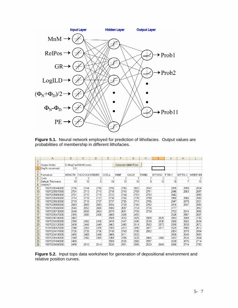
Figure 5.1. Neural network employed for prediction of lithofacies. Output values are probabilities of membership in different lithofacies.

Figure 5.2. Input tops data worksheet for generation of depositional environment and relative position curves.

5- 7

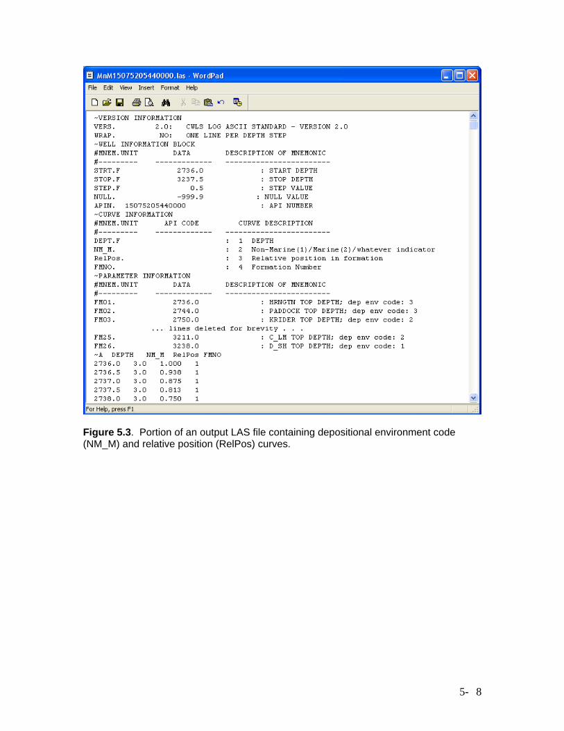
Figure 5.3. Portion of an output LAS file containing depositional environment code (NM_M) and relative position (RelPos) curves.

5- 8

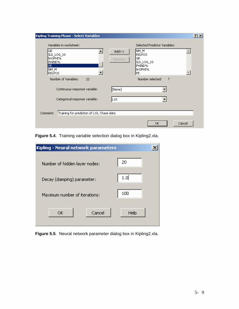
Figure 5.4. Training variable selection dialog box in Kipling2.xla.

Figure 5.5. Neural network parameter dialog box in Kipling2.xla.

5- 9

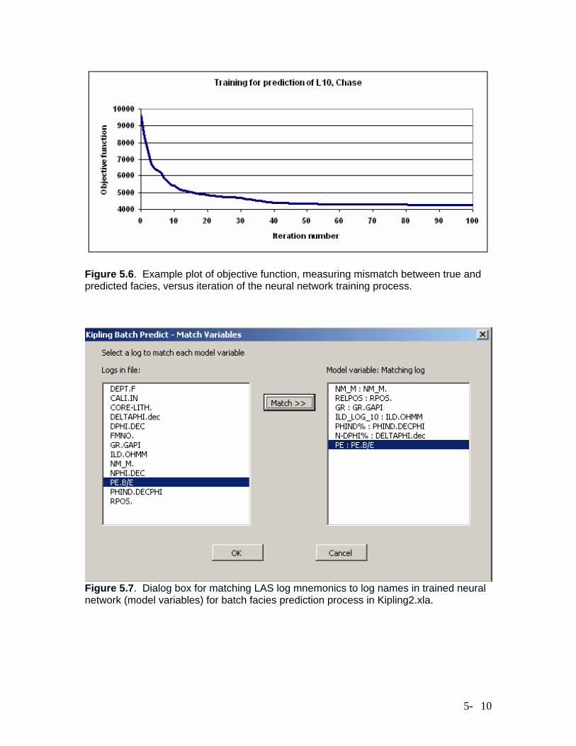
Figure 5.6. Example plot of objective function, measuring mismatch between true and predicted facies, versus iteration of the neural network training process.

Figure 5.7. Dialog box for matching LAS log mnemonics to log names in trained neural network (model variables) for batch facies prediction process in Kipling2.xla.

5- 10

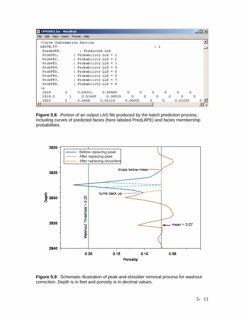
Figure 5.8. Portion of an output LAS file produced by the batch prediction process, including curves of predicted facies (here labeled PredL8PE) and facies membership probabilities.

Figure 5.9. Schematic illustration of peak-and-shoulder removal process for washout correction. Depth is in feet and porosity is in decimal values.

5- 11

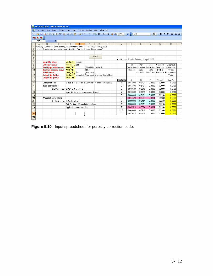
Figure 5.10. Input spreadsheet for porosity correction code.

5- 12

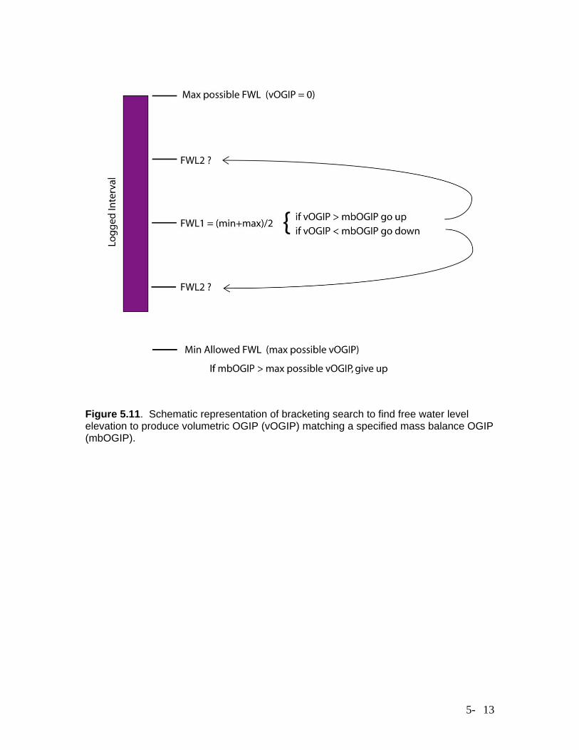
Figure 5.11. Schematic representation of bracketing search to find free water level elevation to produce volumetric OGIP (vOGIP) matching a specified mass balance OGIP (mbOGIP).

5- 13