CHANNEL ESTIMATION REFINEMENT BY TRAINING SEQUENCEEXTENSION AND INTERLEAVER DESIGN

A THESIS SUBMITTED TOTHE GRADUATE SCHOOL OF NATURAL AND APPLIED SCIENCES

OFMIDDLE EAST TECHNICAL UNIVERSITY

BY

SAMET GELINCIK

IN PARTIAL FULFILLMENT OF THE REQUIREMENTSFOR

THE DEGREE OF MASTER OF SCIENCEIN

ELECTRICAL AND ELECTRONICS ENGINEERING

SEPTEMBER 2014

Approval of the thesis:

CHANNEL ESTIMATION REFINEMENT BY TRAINING SEQUENCEEXTENSION AND INTERLEAVER DESIGN

submitted bySAMET GEL INCIK in partial fulfillment of the requirements for thedegree ofMaster of Science in Electrical and Electronics Engineering Depart-ment, Middle East Technical Universityby,

Prof. Dr. Canan ÖzgenDean, Graduate School ofNatural and Applied Sciences

Prof. Dr. Gönül Turhan SayanHead of Department,Electrical and Electronics Engineering

Assoc. Prof. Dr. Ali Özgür YılmazSupervisor,Electrical and Electronics Eng. Dept.,METU

Examining Committee Members:

Prof. Dr.Yalçın TanıkElectrical and Electronics Engineering Dept., METU

Assoc. Prof. Dr. Ali Özgür YılmazElectrical and Electronics Engineering Dept., METU

Prof. Dr. Tolga ÇilogluElectrical and Electronics Engineering Dept., METU

Prof. Dr. T. Engin TuncerElectrical and Electronics Engineering Dept., METU

Prof. Dr. Tolga Mete DumanElectrical and Electronics Engineering Dept., Bilkent University

Date: 04.09.2014

I hereby declare that all information in this document has been obtained andpresented in accordance with academic rules and ethical conduct. I also declarethat, as required by these rules and conduct, I have fully cited and referenced allmaterial and results that are not original to this work.

Name, Last Name: SAMET GELINCIK

Signature :

iv

ABSTRACT

CHANNEL ESTIMATION REFINEMENT BY TRAINING SEQUENCEEXTENSION AND INTERLEAVER DESIGN

Gelincik, Samet

M.S., Department of Electrical and Electronics Engineering

Supervisor : Assoc. Prof. Dr. Ali Özgür Yılmaz

September 2014, 57 pages

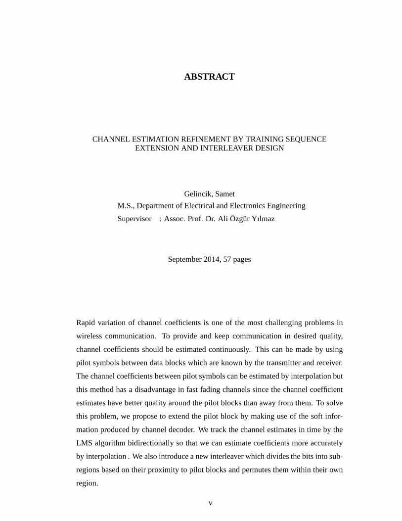
Rapid variation of channel coefficients is one of the most challenging problems in

wireless communication. To provide and keep communicationin desired quality,

channel coefficients should be estimated continuously. This can be made by using

pilot symbols between data blocks which are known by the transmitter and receiver.

The channel coefficients between pilot symbols can be estimated by interpolation but

this method has a disadvantage in fast fading channels sincethe channel coefficient

estimates have better quality around the pilot blocks than away from them. To solve

this problem, we propose to extend the pilot block by making use of the soft infor-

mation produced by channel decoder. We track the channel estimates in time by the

LMS algorithm bidirectionally so that we can estimate coefficients more accurately

by interpolation . We also introduce a new interleaver whichdivides the bits into sub-

regions based on their proximity to pilot blocks and permutes them within their own

region.

v

Keywords: Sum product algorithm, Soft input soft output equalization, channel esti-

mation, least square estimation, least mean square algorithm, interleaver

vi

ÖZ

DENEME DIZISI GENISLETIM I VE KARISTIRICI TASARIMIYLA KANALKESTIRIM I IY ILESTIRMESI

Gelincik, Samet

Yüksek Lisans, Elektrik ve Elektronik Mühendisligi Bölümü

Tez Yöneticisi : Doç. Dr. Ali Özgür Yılmaz

Eylül 2014, 57 sayfa

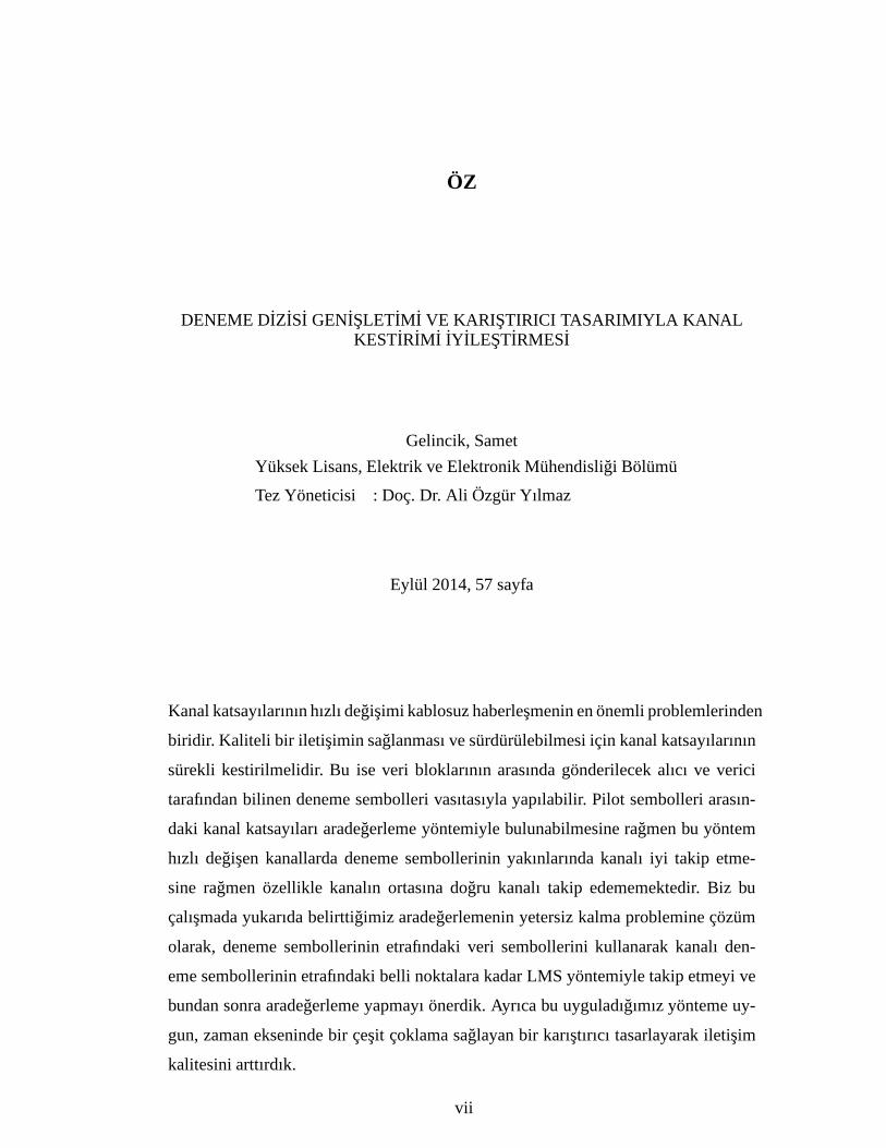
Kanal katsayılarının hızlı degisimi kablosuz haberlesmenin en önemli problemlerinden

biridir. Kaliteli bir iletisimin saglanması ve sürdürülebilmesi için kanal katsayılarının

sürekli kestirilmelidir. Bu ise veri bloklarının arasındagönderilecek alıcı ve verici

tarafından bilinen deneme sembolleri vasıtasıyla yapılabilir. Pilot sembolleri arasın-

daki kanal katsayıları aradegerleme yöntemiyle bulunabilmesine ragmen bu yöntem

hızlı degisen kanallarda deneme sembollerinin yakınlarında kanalı iyi takip etme-

sine ragmen özellikle kanalın ortasına dogru kanalı takip edememektedir. Biz bu

çalısmada yukarıda belirttigimiz aradegerlemenin yetersiz kalma problemine çözüm

olarak, deneme sembollerinin etrafındaki veri sembollerini kullanarak kanalı den-

eme sembollerinin etrafındaki belli noktalara kadar LMS yöntemiyle takip etmeyi ve

bundan sonra aradegerleme yapmayı önerdik. Ayrıca bu uyguladıgımız yönteme uy-

gun, zaman ekseninde bir çesit çoklama saglayan bir karıstırıcı tasarlayarak iletisim

kalitesini arttırdık.

vii

Anahtar Kelimeler: Toplam çarpım algoritması, yumusak girdili yumusak çıktılı

kanal denklestirme, kanal kestirimi, en az kareler kestirimi, en az karesel ortalama

algoritması, karıstırıcı

viii

To my family

ix

ACKNOWLEDGMENTS

First, I would like to thank my supervisor, Ali Özgür Yılmaz,for his continuous

support and mentorship which guide me in both academic and personal life. It is a

great pleasure to work in new and exciting concepts in communications with such a

successful and modest advisor for me.

I am indebted to my first friends in the room C-206 Selim Özgen,Enver Ekmekçi

and Ahmet Elbir for helping me get used to academic environment. Special thanks to

Tugcan Aktas and Pınar Sen for their invaluable friendship and motivating chat in my

hard times. Also, thanks to our new group members Ali Bulut Üçüncü and Alptekin

Yılmaz Yunuscan Gültekin for their pleasant talk. Very special thanks to my friends,

Fatih Özçelik, Nurettin Sezer, Abdülkerim Çengeloglu and especially Mustafa Ergül

and Mehmet Akif Akkus because of their help. Moreover, I thank all of my friends

who are not mentioned here for all their contributions to my personality and my life.

Thanks to the research project supported by Aselsan A.S., Ihad a chance to work with

Ali Özgür Yılmaz and to focus on the core subject of our study which is developed

and presented here.

I thank my family for being so supportive and caring parents.It is priceless to know

that they always stand behind me with their unconditional love. My brother and house

mate Cemal has a very special place in my life. Alongside of our invaluable memories

since our childhood, I am grateful for his relaxing and cheerful personality which has

a healing effect on me in my hard times.

x

TABLE OF CONTENTS

ABSTRACT . . . . . . . . . . . . . . . . . . . . . . . . . . . . . . . . . . . . v

ÖZ . . . . . . . . . . . . . . . . . . . . . . . . . . . . . . . . . . . . . . . . . vii

ACKNOWLEDGMENTS . . . . . . . . . . . . . . . . . . . . . . . . . . . . . x

TABLE OF CONTENTS . . . . . . . . . . . . . . . . . . . . . . . . . . . . . xi

LIST OF TABLES . . . . . . . . . . . . . . . . . . . . . . . . . . . . . . . . xiv

LIST OF FIGURES . . . . . . . . . . . . . . . . . . . . . . . . . . . . . . . . xv

LIST OF ABBREVIATIONS . . . . . . . . . . . . . . . . . . . . . . . . . . . xviii

CHAPTERS

1 INTRODUCTION . . . . . . . . . . . . . . . . . . . . . . . . . . . 1

2 BACKGROUND INFORMATION . . . . . . . . . . . . . . . . . . . 5

2.1 Wireless Channel Characterization . . . . . . . . . . . . . . 5

2.1.1 Some Wireless Channel Features . . . . . . . . . . 5

2.1.2 Channel Model . . . . . . . . . . . . . . . . . . . 6

2.2 The HF Communication . . . . . . . . . . . . . . . . . . . . 7

2.2.1 Propagation Mechanism . . . . . . . . . . . . . . 7

2.2.2 HF Channel . . . . . . . . . . . . . . . . . . . . . 8

2.3 Channel Estimation Techniques . . . . . . . . . . . . . . . . 9

xi

2.3.1 Least Squares Estimation . . . . . . . . . . . . . . 10

2.3.2 Maximum Likelihood Estimation . . . . . . . . . 10

2.4 Equalizer . . . . . . . . . . . . . . . . . . . . . . . . . . . . 11

2.4.1 Interleaver . . . . . . . . . . . . . . . . . . . . . . 12

2.5 System Model . . . . . . . . . . . . . . . . . . . . . . . . . 13

2.5.1 General Model . . . . . . . . . . . . . . . . . . . 13

2.5.2 Specific Model . . . . . . . . . . . . . . . . . . . 16

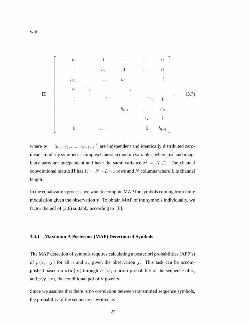
3 THE SUM PRODUCT ALGORITHM AND SOFT-INPUT SOFT-OUTPUT (SISO) EQUALIZER . . . . . . . . . . . . . . . . . . . . 17

3.1 Introduction . . . . . . . . . . . . . . . . . . . . . . . . . . 17

3.2 Sum Product Algorithm . . . . . . . . . . . . . . . . . . . . 18

3.3 A Specific Example . . . . . . . . . . . . . . . . . . . . . . 19

3.4 Soft-Input Soft-Output (SISO) Equalizer . . . . . . . . . . . 21

3.4.1 Maximum A Posteriori (MAP) Detection of Sym-bols . . . . . . . . . . . . . . . . . . . . . . . . . 22

3.4.2 Graph-Based Detection Algorithm . . . . . . . . . 24

4 CHANNEL ESTIMATION, TRACKING AND INTERLEAVER DE-SIGN IN TIME DOMAIN . . . . . . . . . . . . . . . . . . . . . . . 29

4.1 Introduction . . . . . . . . . . . . . . . . . . . . . . . . . . 29

4.2 System Model for Receiver Part . . . . . . . . . . . . . . . . 30

4.3 Channel Estimation From Mini Probe . . . . . . . . . . . . . 31

4.4 Extension of Pilot Blocks . . . . . . . . . . . . . . . . . . . 33

4.5 Channel Tracking With LMS . . . . . . . . . . . . . . . . . 38

4.6 Interleaver Design . . . . . . . . . . . . . . . . . . . . . . . 44

xii

4.7 Results . . . . . . . . . . . . . . . . . . . . . . . . . . . . . 47

5 CONCLUSION . . . . . . . . . . . . . . . . . . . . . . . . . . . . . 53

REFERENCES . . . . . . . . . . . . . . . . . . . . . . . . . . . . . . . . . . 55

xiii

LIST OF TABLES

TABLES

xiv

LIST OF FIGURES

FIGURES

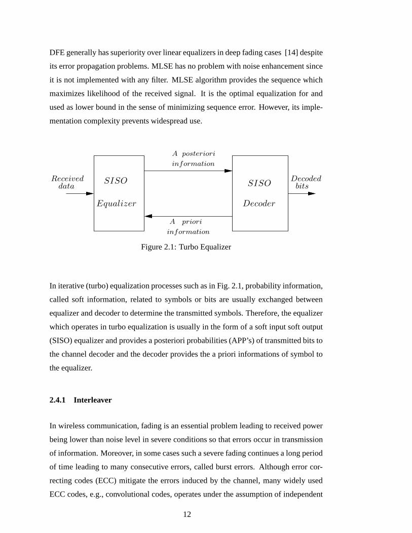
Figure 2.1 Turbo Equalizer . . . . . . . . . . . . . . . . . . . . . . . . . . . 12

Figure 2.2 Reference system model using adaptive turbo equalization in the

receiver . . . . . . . . . . . . . . . . . . . . . . . . . . . . . . . . . . . 14

Figure 2.3 Transmitted signal frame . . . . . . . . . . . . . . . . . . . .. . . 16

Figure 3.1 A factor graph forg (x1, x2, ...xn) . . . . . . . . . . . . . . . . . . 18

Figure 3.2 A factor graph forf (x1, x2, x3, x4, x5) . . . . . . . . . . . . . . . 20

Figure 3.3 Some part of the factor graph respect to 3.21, whenthe interference

exist betweenxn andxk if | k − n |∈ 1,2 . . . . . . . . . . . . . . . . . . 25

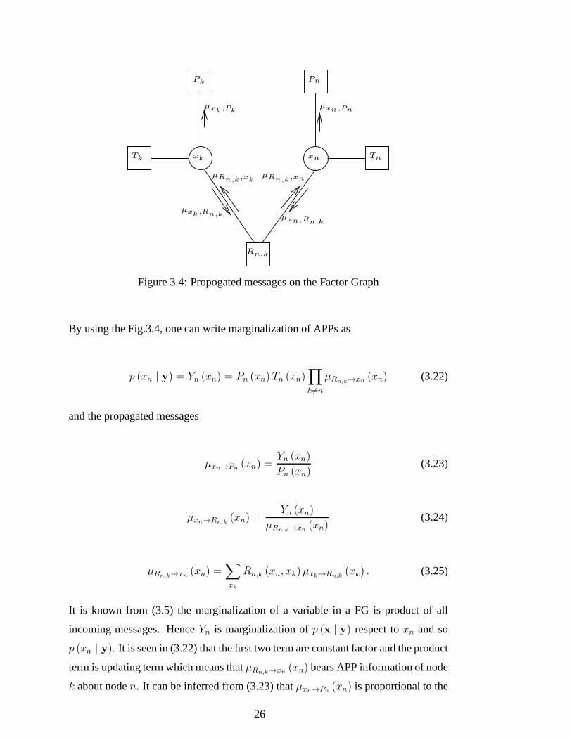
Figure 3.4 Propogated messages on the Factor Graph . . . . . . . .. . . . . . 26

Figure 4.1 Channel estimation and tracking system model . . .. . . . . . . . 30

Figure 4.2 Detailed representation of pilot blocks and a transmitted sequence . 31

Figure 4.3 Interpolation performance along a packet under 1Hz Doppler spread

at SNR 8 dB . . . . . . . . . . . . . . . . . . . . . . . . . . . . . . . . . 34

Figure 4.4 Interpolation performance of along a packet under 5 Hz Doppler

spread at 8 dB . . . . . . . . . . . . . . . . . . . . . . . . . . . . . . . . 34

Figure 4.5 Log-likelihood-ratios of encoded bits under 5 HzDoppler spread

at SNR=8 dB for 4QAM . . . . . . . . . . . . . . . . . . . . . . . . . . . 35

xv

Figure 4.6 Log-likelihood-ratios of encoded bits under 5 HzDoppler spread

at SNR=8 dB for BPSK . . . . . . . . . . . . . . . . . . . . . . . . . . . 36

Figure 4.7 Log-likelihood-ratios of encoded bits of the first data block under

5 Hz Doppler spread at 8 dB . . . . . . . . . . . . . . . . . . . . . . . . . 36

Figure 4.8 Log-likelihood-ratios of encoded bits of the first data block under

5 Hz Doppler spread at 8 dB . . . . . . . . . . . . . . . . . . . . . . . . . 37

Figure 4.9 Iteratively extended pilot regions . . . . . . . . . . .. . . . . . . 38

Figure 4.10 Representation of extended training points . . .. . . . . . . . . . 38

Figure 4.11 Comparison interpolated channel estimations as a function of iter-

ation number at SNR=10 dB . . . . . . . . . . . . . . . . . . . . . . . . . 40

Figure 4.12 Performance comparison with and without channel estimation re-

finement . . . . . . . . . . . . . . . . . . . . . . . . . . . . . . . . . . . 41

Figure 4.13 Comparison of extension numbers for 4QAM at 3Hz Doppler spread

41

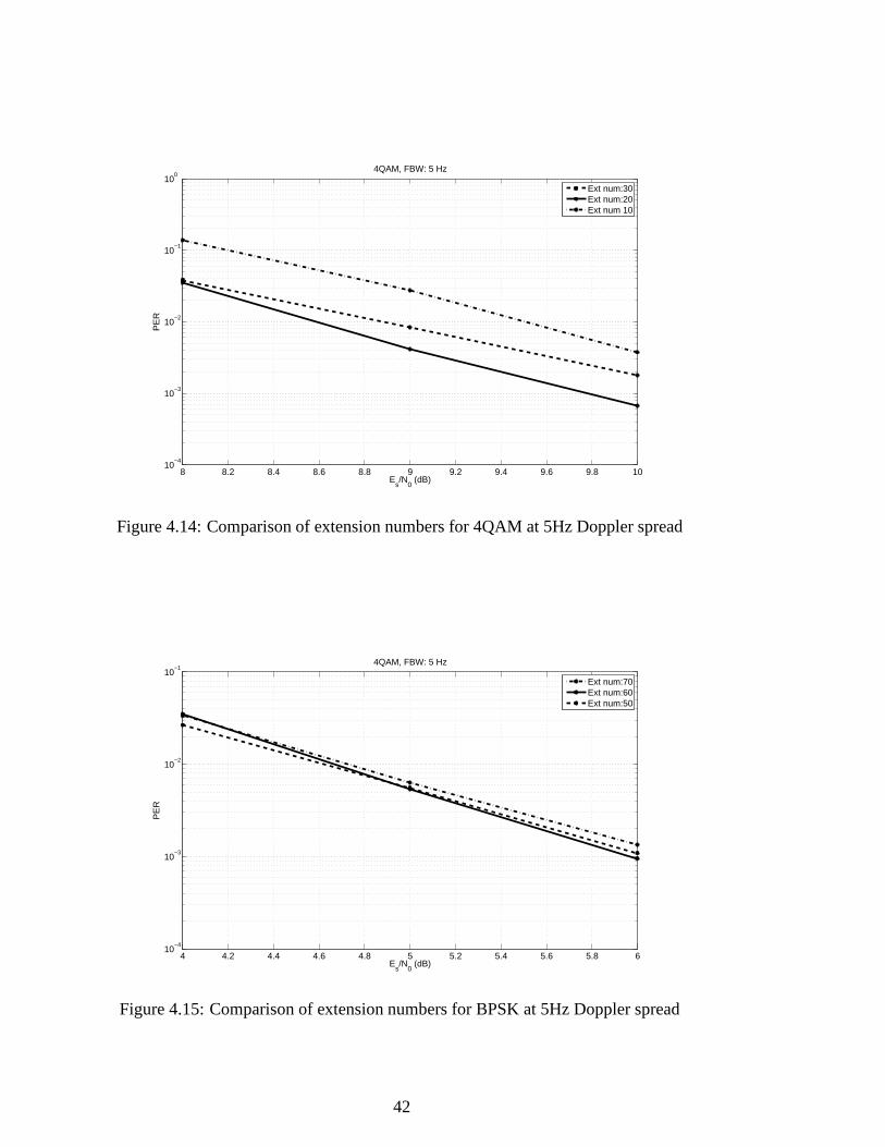
Figure 4.14 Comparison of extension numbers for 4QAM at 5Hz Doppler spread 42

Figure 4.15 Comparison of extension numbers for BPSK at 5Hz Doppler spread 42

Figure 4.16 Experimentally Optimum LMS coefficients for BPSK at 5 Hz Doppler

Spread . . . . . . . . . . . . . . . . . . . . . . . . . . . . . . . . . . . . 43

Figure 4.17 Experimentally Optimum LMS coefficients for BPSK at 7 Hz Doppler

Spread . . . . . . . . . . . . . . . . . . . . . . . . . . . . . . . . . . . . 43

Figure 4.18 Extrinsic LLR of a data block produced by equalizer at SNR=8 dB

after initial equlization . . . . . . . . . . . . . . . . . . . . . . . . . . . .44

Figure 4.19 Extrinsic LLR of a data block produced by decoderat SNR=8 dB

after initial equalization . . . . . . . . . . . . . . . . . . . . . . . . . . .45

Figure 4.20 Interleaving Process . . . . . . . . . . . . . . . . . . . . . .. . . 46

xvi

Figure 4.21 Performance comparison of various schemes for 4QAM at FBW 1

Hz . . . . . . . . . . . . . . . . . . . . . . . . . . . . . . . . . . . . . . 48

Figure 4.22 Performance comparison of various schemes for 4QAM at FBW 3

Hz . . . . . . . . . . . . . . . . . . . . . . . . . . . . . . . . . . . . . . 48

Figure 4.23 Performance comparison of various schemes for BPSK at FBW 5 Hz 49

Figure 4.24 Performance comparison of various schemes for 4QAM at FBW 5

Hz . . . . . . . . . . . . . . . . . . . . . . . . . . . . . . . . . . . . . . 49

Figure 4.25 Performance comparison of various schemes for BPSK at FBW 7 Hz 50

Figure 4.26 Performance comparison of various schemes for 4QAM at FBW 7

Hz . . . . . . . . . . . . . . . . . . . . . . . . . . . . . . . . . . . . . . 51

xvii

LIST OF ABBREVIATIONS

APP A Posteriori Probability

AR Auto-regressive

AWGN Additive White Gaussian Noise

PER Packet-Error-Rate

BPSK Binary Phase Shift Keying

BCJR Bahl-Cocke-Jelinek-Raviv

FDE Frequency Domain Equalization

GMP Gaussian Message Passing

ISI Inter-Symbol Interference

JG Joint Gaussian

LMMSE Linear Minimum Mean Square Error

LLR Log-likelihood Ratio

MSE Mean Square Error

pdf Probability Density Function

PSD Power Spectral Density

PSK Phase Shift Keying

QAM Quadrature Amplitude Modulation

rRC Root-Raised-Cosine

SC-FDE Single Carrier Frequency Domain Equalization

SISO Soft in Soft Out

SNR Signal-to-Noise Ratio

ZMCSCG Zero Mean Circularly Symmetric Complex Gaussian

xviii

CHAPTER 1

INTRODUCTION

Signals transmitted through wireless channels are exposedto various adverse effects

due to the nature of the wireless medium. One of these effectsis multipath propaga-

tion which is the result of reflection, refraction or diffraction. Multipath propagation

reproduces many copies of the transmitted signal where a receiver antenna observes

multiple echoes in different delays and attenuations. Whenthe multipath delay is

greater than the symbol duration, interference across symbols (inter-symbol inter-

ference (ISI)) forms. Multipath propagation also causes fluctuation in received sig-

nal power which is called fading. Furthermore, changes of communication medium

makes the channel time varying. To reconstruct the transmitted signal at the receiver

side channel estimation and equalization must be carried out.

In many scenarios channel estimation is an integral part of the receiver design. In the

literature, there are three different channel estimation techniques: blind, semi blind

and training based. Blind channel estimation [28] method isbased on estimating the

channel using known statistics about the channel and input sequence, not through

known symbols. However, it has some disadvantages such as convergence, latency,

phase ambiguity etc. To overcome such problems, semi blind channel estimation

methods [28] are suggested so that fast and robust estimation can be provided by

means of using known symbols and known statistics about datasymbols [11]. The

semi blind estimation can also be used efficiently in estimating fast fading channels

and has superiority over training based and blind channel estimation separately [11].

Training-based channel estimation is executed in various ways through transmission

of symbols known both to transmitter and receiver. Some of the techniques used

1

with training based estimation are Least Squares [31], correlation estimation [5], ML

estimation [30]. As an example, training based channel estimation is used in Global

System for Mobile Communication (GSM) [15] and EDGE [16].

Training based channel estimation is used effectively in case of slow time variation of

the channel through pilot sequences transmitted periodically. In this case, the channel

is estimated at pilot regions and then interpolated for the data regions by various inter-

polators such as linear [6], Wiener filtering [7]. This approach is used in IS-136 [3].

However, when the time variation rate of the channel increases, interpolation aided

training based channel estimation is not effective especially because of throughput

inefficiency since it requires transmitting pilot sequences more frequently. To enable

channel estimation in relatively fast fading channels, there are several methods in the

literature for iterative receivers. In [27] and [24],a dataaided channel estimation

method is proposed in which the channel is iteratively estimated through soft infor-

mation of the channel decoder by using some techniques such as LMS, RLS, Kalman

filtering. As an alternative to those methods, we propose another data directed train-

ing based channel estimation method. The method iteratively extends pilot sequence

to portions of data which is estimated through the soft information produced by de-

coder. With this "extended training sequence", the channelcan be tracked bidirec-

tionally inside the extended training sequence regions. Then, interpolation provides

better quality channel estimation along a whole packet.

In Chapter 2, the background information needed through thethesis can be found.

In Chapter 3, both the sum product (SP) algorithm which is an implementation of

soft input soft output (SISO) equalizer and the utilized SISO equalizer structure is

described. In Chapter 4, channel estimation with the least squares (LS) algorithm,

the pilot extension idea, tracking of the channel with the LMS algorithm, interleaver

design are explained and related results are provided. Conclusions follow in chapter

5.

The employed notations are organized as follows. Lower caseletters (e.g.,x) repre-

sents scalars, bold letters (e.g.,x) denote vectors, bolded upper case letters (e.g.,X)

denote matrices. For a given vector random variablex, Rx denote its autocorrela-

tion matrix. The indicators()H , ()∗, andE{} denote Hermitian transpose, conjugate

2

transpose and expectation operations respectively. The matrix I represents the iden-

tity matrix of proper size.

3

4

CHAPTER 2

BACKGROUND INFORMATION

2.1 Wireless Channel Characterization

2.1.1 Some Wireless Channel Features

Wireless transmission medium has many features different from those of fixed or

wired channels and these features are the consequence of mobility and specific nature

of the surrounding medium.

Multipath propagation is a very important phenomenon that has role on many prob-

lems which arise in wireless communication. During a wireless transmission, a trans-

mitter and receiver may have a direct path between each otherand it is called the line

of sight path (LOS). However, the signal reaches the receiver through many different

paths and this phenomenon is called multipath propagation resulting from many in-

teracting objects surrounding the transmitter and receiver like houses, walls, doors or

windows which the signal reflects and/or diffracts through them. These signals have

various amplitude, phase and delay.

The deviation of a multipath signal experienced in relativephase of a frequency com-

ponent or in amplitude is defined as fading and results in attenuation of the signal.

The multipath components of a signal causes interference and this interference can

be constructive or destructive depending on the phase of thearriving multipath com-

ponents. Instantaneous deviation of the signal level is defined as small scale fading.

Large- scale fading occurs if there is an obstacle in the propagation path so that one

or many multipath components are attenuated greatly with the result of preventing the

5

communication. The small and large scale fading are combined at the receiver and

in practice, it results in changing the channel coefficientswith time and sometimes

signal power undergo noise level with the consequence of symbol error in an uncoded

structure.

The maximum delay between multipath components of a symbol is defined as delay

spread,Tm. Multipath signal components coming from different path lengths may

cause interference at the receiver if a multipath componentof a signal arrives the

antenna at the same time with any subsequent signal. This situation arises if one of

the delays between multipath components of a transmitted symbol is greater than a

symbol duration. This phenomenon is called inter-symbol interference (ISI).

Movements of the transmitter and receiver or changes in the surrounding medium

leads to variation of the multipath components’ properties. This dynamic behaviour

of the channel impulse response is usually characterized byDoppler spread of the

channel which roughly describes the rate of change for the channel impulse response

components. Assuming wide sense stationary channel impulse response, the varia-

tion in time is reflected in power spectral density (PSD). In our simulations, we will

consider a Gaussian shaped PSD where the twice the standard deviationσ of the PSD

will be referred to as fading bandwidth (FBW). FBW is also a measure for channel

coherence timeTc. The coherence time is qualitatively defined as the range of values

over which the autocorrelation of channel taps in time is nonzero. The relationship

between the channel coherence time and FBW is

Tc ≈1

FBW. (2.1)

2.1.2 Channel Model

In this thesis, we consider a channel model characterized asa discrete time baseband

equivalent channel with the assumption that required conditions such as proper sam-

pling and filtering are in effect [26]. The discrete time model for a time varying

channel is

6

hn = [hn,0, hn,1, ..., hn,L−1] (2.2)

wheren indicates the sampling timenT + τ0, T andτ0 are symbol duration and an

arbitrary time offset. The index k inhn,k indicates the response of channel with delay

kT at the time instantnT + τ0 andL indicates the total channel length.

In the time invariant case, the time index n is dropped since the channel is constant

the whole observation time so that

h = [h0, h1, ..., hL−1] . (2.3)

2.2 The HF Communication

The High Frequency (HF) band is defined as the electromagnetic spectrum between

3 MHz and 30 MHz, which corresponds to wavelengths between 10m and 100 m.

The radio communication which is performed in this frequency band is called HF

communication. The detailed information about HF communication can be found in

[18] and [17].

HF communication is very often used for military purposes. Military communica-

tion standards are being developed by NATO (North AthlanticTreaty Organization),

and by US DoD (United States Department of Defence). The STANAG (Standard-

ization Agreement) series is published by NATO , the MIL-STD(Military Standard)

series is published by US DoD. With the introduction of some new standards such as

STANAG 4539, Military Standard 188110-C, the performance is improved in terms

of availability and data rates.

2.2.1 Propagation Mechanism

There are two major propagation mechanisms for electromagnetic waves in the HF

band. One of them is ground wave in which the waves propagate along the surface

of the earth. The other one is sky wave in which the waves are reflected back to the

7

earth from the ionosphere. Transmission frequency and conductivity of the surface of

the earth determines the propagation range of the ground wave.

Sky wave is used for communication distances of at least 50 kmby using one or more

reflection between earth and ionosphere layers. When the electromagnetic waves

from the sun is absorbed by the athmosphere, molecules are ionized. The density

profile of different types of molecules, the solar zenith angle and the strength of the

ionizing electromagnetic waves determine the ionization which is concentrated in

layers or regions. Since ionization depends on the solar zenith angle, it is denser

during day than during night, and denser in summer than in winter. The solar activity

and the 11-year sunspot cycle change the ionization density.

The lowest altitude, between 60-90 km, of the ionosphere corresponds to layer D and

it has lower electron density respect to layer D and F so that does not reflect the radio

waves. However, it absorbs the energy of waves. The middle layer is layer E and the

altitude is between 90 and 120 km. The layer F is highest altitude and it includes the

altitude between 200 and more than 500 km. The E and F regions electron density

is enough to refract electromagnetic waves in HF range so these two regions act as a

reflector for HF communication.

The received noise in HF frequencies consists of man made noise, galactic noise and

athmospheric noise (static discharge). This noise is investigated in [13] and it may

has a bursty nature. However, it can be modelled as band-limited additive White

Gaussian noise with a simplifying assumption. More detailscan be found in [20].

2.2.2 HF Channel

The transmitter and receiver are not moving (or moving slowly relative to the wave-

length) in ionospheric HF communication system. However, the electromagnetic

waves are being reflected from large number of randomly moving ions. This means

that the Doppler shift can be modelled by Gaussian distribution [22]. This model is

verified experimentally by Watterson, Juroshek and Bensemain [29]. The model is

referred as Watterson model in literature.

The Watterson channel is a two tap channel with the delay spread values quite large

8

in the vicinity of a few milliseconds. The taps are independent and have equal power

with the Gaussian PSD.

Assuming the mean of Doppler shift is zero, the Gaussian Doppler spectrum can be

written as

Sh (υ) =1√2πσ2

υ

exp

(−

υ2

2σ2

)(2.4)

whereσ2υ is the variance of the Doppler shift. For a fading channel which has Gaus-

sian power spectral density, we define the Doppler spread or fading bandwith (FBW)

as twice of the standard deviation of the Doppler shift

FBW = 2συ. (2.5)

2.3 Channel Estimation Techniques

In the thesis, a data directed training based channel estimation technique will be used.

Hence, the channel estimation method is based on using not only the known symbols

and their corresponding observations, but also on observations of unknown data. It

is imperative that training based channel estimation is basis of data directed channel

estimation. Training based channel estimation is applied for time-invariant channels

and in case of very short pilot sequence duration so that the channel varies slowly.

Assuming a training sequencex = [x0, x1, ..., xN ], the corresponding outputy =

[y0, y1, ...., yN+L−1] and the channelh = [h0, h1, ..., hL−1] , our discrete time system

model is given in matrix form for the time-invariant case as [2]

y = Xh+w (2.6)

whereX is anN + L − 1 × L matrix whose rows are shifts of training sequence

andw = [w0, w1, ..., wN+L−1] is composed of circularly symmetric complex additive

white Gaussian noise samples.

9

2.3.1 Least Squares Estimation

Least Squares (LS) channel estimation can be obtained from

hLS = argminh (y −Xh)H (y −Xh) . (2.7)

The size of vectory is N which is the number of received signals affected by only

the training symbols. The LS estimation of channel can be found by the equation [2]

hLS =(XHX

)−1XHy. (2.8)

2.3.2 Maximum Likelihood Estimation

With maximum likelihood (ML) channel estimation, the coefficients which maxi-

mizes the likelihood of the received signal is searched for:

hML = argmaxhp (y | h) . (2.9)

For complex Gaussian noise, the solution can be obtained by maximizing the equation

given in [2]

hML = argmaxh (y−Xh)H R−1w (y −Xh) (2.10)

which is related to the logarithm of the ML function whereRw is the covariance

matrix of noise. In that case, the ML estimate of the channel is given in [2] as

hML =(XHR−1

w X)−1 (

XHR−1w

)y. (2.11)

However, in case of zero mean circularly symmetric white Gaussian noise,Rw = N0I

and the ML estimate can be calculated with

10

hML =(XHX

)−1 (XH)y. (2.12)

It is seen from (2.12) and (2.8) that two estimation techniques is matched if the noise

is zero mean circularly symmetric white Gaussian noise.

2.4 Equalizer

From section 2.1.1, it is known that ISI occurs if delay spread Tm is greater than sym-

bol durationT . ISI prevents correct symbol and bit decoding unless special measures

are not taken even in high signal-to-noise ratios (SNR). In abroad manner, any signal

processing method which alleviates ISI is called equalization. Equalization can be

implemented through one of filtering, sequence estimation or iterative techniques.

There are two main types of equalizers in the literature: linear and non-linear. Some

linear equalizer types can suffer from noise enhancement [14] which results in SNR

degradation even though ISI is completely eliminated. Non linear equalization meth-

ods have less noise enhancement but it has larger implementation complexity. Equal-

ization techniques requires channel impulse response to mitigate the ISI. In time vary-

ing cases, the equalizer tracks the change in channel with the aid of training symbols

through some updating methods, i.e. LMS, RLS, Kalman filtering etc., which are

categorized as adaptive equalization.

Two of the popular linear equalizers are zero forcing (ZF) and minimum mean square

(MMSE) equalizers. ZF equalizers eliminate all ISI introduced by the channel but has

trouble with noise enhancements. MMSE equalizer works in the sense which min-

imizes mean square error between the transmitted symbols and their corresponding

equalizer outputs so that its noise enhancement problem is less than ZF equalizer but

it does not eliminate all ISI. In short, the MMSE equalizers balance ISI mitigation

and noise enhancement.

Nonlinear equalizer examples are decision feedback equalizer (DFE) and maximum

likelihood sequence estimaton (MLSE). DFE uses previouslyestimated symbols to al-

leviate ISI through a feedback filter and does not suffer fromnoise enhancement. Also

11

DFE generally has superiority over linear equalizers in deep fading cases [14] despite

its error propagation problems. MLSE has no problem with noise enhancement since

it is not implemented with any filter. MLSE algorithm provides the sequence which

maximizes likelihood of the received signal. It is the optimal equalization for and

used as lower bound in the sense of minimizing sequence error. However, its imple-

mentation complexity prevents widespread use.

Equalizer Decoder

priori

posteriori

information

information

A

A

Receiveddata bits

DecodedSISOSISO

Figure 2.1: Turbo Equalizer

In iterative (turbo) equalization processes such as in Fig.2.1, probability information,

called soft information, related to symbols or bits are usually exchanged between

equalizer and decoder to determine the transmitted symbols. Therefore, the equalizer

which operates in turbo equalization is usually in the form of a soft input soft output

(SISO) equalizer and provides a posteriori probabilities (APP’s) of transmitted bits to

the channel decoder and the decoder provides the a priori informations of symbol to

the equalizer.

2.4.1 Interleaver

In wireless communication, fading is an essential problem leading to received power

being lower than noise level in severe conditions so that errors occur in transmission

of information. Moreover, in some cases such a severe fadingcontinues a long period

of time leading to many consecutive errors, called burst errors. Although error cor-

recting codes (ECC) mitigate the errors induced by the channel, many widely used

ECC codes, e.g., convolutional codes, operates under the assumption of independent

12

bit/symbol errors. Interleaving is an effective solution to roughly create such a sce-

nario with burst errors. Interleaver is defined as a single input single output device

which takes the symbol sequence in a fixed alphabet and produces the same sequence

in a different order. The classical usage of interleaver is to separate the consecutive

bits to minimize the burst error probability by way of transforming the channel as if

errors occur in regions apart from each other. A similar scenario is needed in turbo

decoding and equalization. Hence interleaving is usually present in turbo decoding

and equalization systems [26].

We will utilize block interleavers in this work. In a block interleaver data is written

in row-wise in a matrix form and read in column-wise from thatmatrix. A pseudo

random block interleaver is a sort of block interleaver in which data is written a se-

quential manner and read out in a pseudo random order.

2.5 System Model

2.5.1 General Model

Consider the system shown in Fig. 2.2. A block of data bitsbl ∈ {1, 0} are convolu-

tionally encoded with a rateRc to form coded bitscp′ ∈ {1, 0}, then the coded bits are

interleaved tocp by employing a permutation functionΠ (.). Throughout this work,

gray mapping is used for modulation whereQ consecutive coded bitsc(n−1)Q+i, i ∈

{1, 2, .., Q} are combined to form a symbolzn in S = {s1, s2, ....., s2Q}. The constel-

lations are phase shift keying (PSK) and quadrature amplitude modulation (QAM). In

addition to data symbols, training and synchronization symbols which are known by

receiver are added to data sequence to form transmitted symbolsxn, n ∈ {1, 2, ..., N}.

Thenxn are modulated with a carrier at a symbol ratefs symbols per second. Sym-

bol spaced discrete time model for sending the symbolsxn through the intersymbol

interference (ISI) channel produces the received symbols

yn = hTxn + wn (2.13)

13

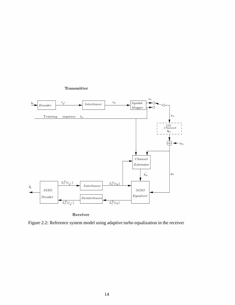
hn

Channel

Estimator

EncoderMapper

Training sequence tn

wn

zn

Interleaver

ChannelISI

Transmitter

Receiver

bl

blcp

Equalizer

SISO

Interleaver

Decoder

SISO

xn

yn

LEe (cp)

LDe (c

p′ )

LEe (c

p′ )

LDe (cp)

Deinterleaver

cp′ Symbol

hn

Figure 2.2: Reference system model using adaptive turbo equalization in the receiver

14

wherehn = [hn,0, ...., hn,L−1] is the time varying channel impulse response (CIR) at

time n with lengthL andxn = [xn, xn−1, ..., xn−L+1]. The scalarwn denotes inde-

pendent and identically distributed zero mean circularly symmetric complex Gaussian

random variables, where real and imaginary parts are independent and have the same

varianceσ2 = N0/2. It is more compact to write the transmission model in matrix

form. Thereby, in case of the transmitted symbol sequencex = [x1, x2, ..., xN ], the

received signal can be written

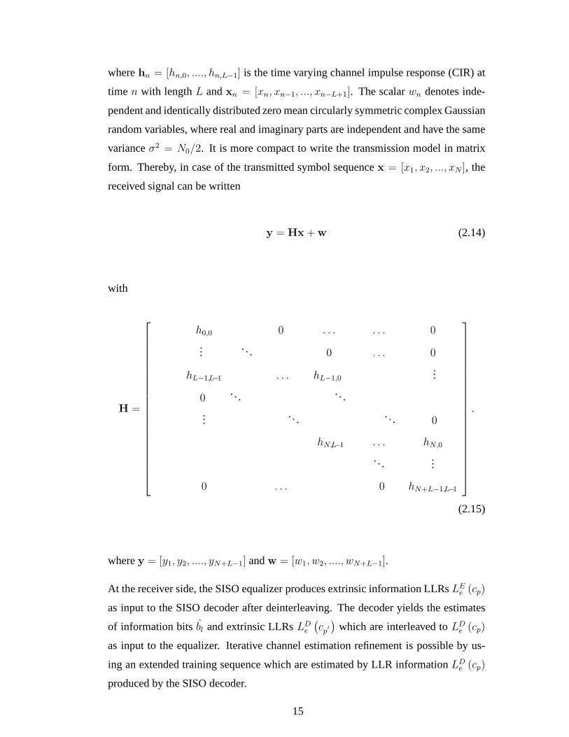
y = Hx+w (2.14)

with

H =

h0,0 0 . . . . . . 0

.... . . 0 . . . 0

hL−1,L−1 . . . hL−1,0...

0. . . . . .

.... . . . . . 0

hN,L−1 . . . hN,0

. . ....

0 . . . 0 hN+L−1,L−1

.

(2.15)

wherey = [y1, y2, ...., yN+L−1] andw = [w1, w2, ...., wN+L−1].

At the receiver side, the SISO equalizer produces extrinsicinformation LLRsLEe (cp)

as input to the SISO decoder after deinterleaving. The decoder yields the estimates

of information bitsbl and extrinsic LLRsLDe

(cp′)

which are interleaved toLDe (cp)

as input to the equalizer. Iterative channel estimation refinement is possible by us-

ing an extended training sequence which are estimated by LLRinformationLDe (cp)

produced by the SISO decoder.

15

2.5.2 Specific Model

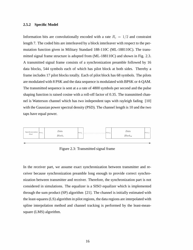
Information bits are convolutionally encoded with a rateRc = 1/2 and constraint

length 7. The coded bits are interleaved by a block interleaver with respect to the per-

mutation function given in Military Standard 188-110C (ML-188110C). The trans-

mitted signal frame structure is adopted from (ML-188110C)and shown in Fig. 2.3.

A transmitted signal frame consists of a synchronization preamble followed by 16

data blocks, 544 symbols each of which has pilot block at bothsides. Thereby a

frame includes 17 pilot blocks totally. Each of pilot block has 68 symbols. The pilots

are modulated with 8 PSK and the data sequence is modulated with BPSK or 4-QAM.

The transmitted sequence is sent at a a rate of 4800 symbols per second and the pulse

shaping function is raised cosine with a roll-off factor of 0.35. The transmitted chan-

nel is Watterson channel which has two independent taps withrayleigh fading [10]

with the Gaussian power spectral density (PSD). The channellength is 10 and the two

taps have equal power.

Pilot1 Pilot2 Pilot16 Pilot17

Data

Block16Part

Data

Block1

Synchronization

Figure 2.3: Transmitted signal frame

In the receiver part, we assume exact synchronization between transmitter and re-

ceiver because synchronization preamble long enough to provide correct synchro-

nization between transmitter and receiver. Therefore, thesynchronization part is not

considered in simulations. The equalizer is a SISO equalizer which is implemented

through the sum product (SP) algorithm [21]. The channel is initially estimated with

the least-squares (LS) algorithm in pilot regions, the dataregions are interpolated with

spline interpolation method and channel tracking is performed by the least-mean-

square (LMS) algorithm.

16

CHAPTER 3

THE SUM PRODUCT ALGORITHM AND SOFT-INPUT

SOFT-OUTPUT (SISO) EQUALIZER

3.1 Introduction

In our work, our interest is HF communication. It is known that HF channel is mod-

elled as a time varying inter-symbol interference (ISI) channel [23] so that an equal-

izer is utilized in the receiver side to alleviate ISI. Our receiver (in Section 2.5)

performs turbo equalization which exchanges soft information between equalizer and

decoder. Therefore our equalizer should be a soft in soft out(SISO) component,

which is also called SISO equalizer. The early SISO equalizers were based on trel-

lis based algorithms [4] and [12]. However, the number of trellis states becomes

excessive size when the channel impulse response (CIR) is very large and the signal

constellation is large [25]. This makes trellis based SISO equalization impractical

for HF communication since the corresponding channel lengths are long generally.

Despite some performance degradation suboptimal SISO equalizers based on soft ISI

cancellation and linear filtering methods are utilized to overcome practical difficul-

ties.

The SISO equalization can provide marginal a posteriori probabilities (MAP) of the

transmitted symbols with soft ISI cancellation. In so doing, one has to marginalize

the joint probability density function of transmitted vector given the received vector in

order to compute the MAP of transmitted symbols. SISO equalization implemented

on a suitable factor graph (FG) is an attractive option in thesense of complexity and

practicality.

17

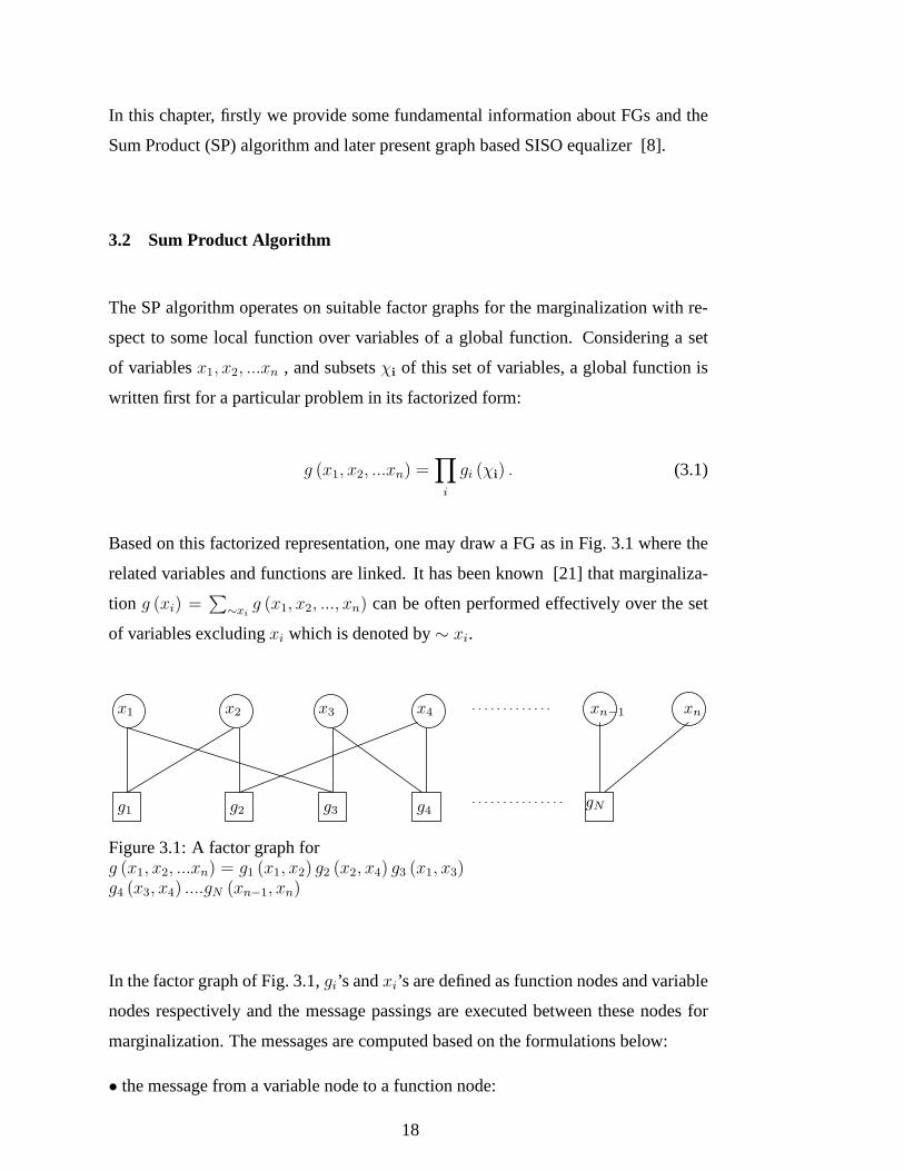
In this chapter, firstly we provide some fundamental information about FGs and the

Sum Product (SP) algorithm and later present graph based SISO equalizer [8].

3.2 Sum Product Algorithm

The SP algorithm operates on suitable factor graphs for the marginalization with re-

spect to some local function over variables of a global function. Considering a set

of variablesx1, x2, ...xn , and subsetsχi of this set of variables, a global function is

written first for a particular problem in its factorized form:

g (x1, x2, ...xn) =∏

i

gi (χi) . (3.1)

Based on this factorized representation, one may draw a FG asin Fig. 3.1 where the

related variables and functions are linked. It has been known [21] that marginaliza-

tion g (xi) =∑

∼xig (x1, x2, ..., xn) can be often performed effectively over the set

of variables excludingxi which is denoted by∼ xi.

gNg4

x3 x4x2x1

g1 g2

xn−1 xn

g3

Figure 3.1: A factor graph forg (x1, x2, ...xn) = g1 (x1, x2) g2 (x2, x4) g3 (x1, x3)g4 (x3, x4) ....gN (xn−1, xn)

In the factor graph of Fig. 3.1,gi’s andxi’s are defined as function nodes and variable

nodes respectively and the message passings are executed between these nodes for

marginalization. The messages are computed based on the formulations below:

• the message from a variable node to a function node:

18

µxi→gj (xi) =∏

gk∈n(xi)\{gj}

µgk→xi(xi) , (3.2)

• the message from a function node to a variable node:

µgj→xi(xi) =

∑

∼{xi}

gj (χj)

∏

xk∈n(gj)\{xi}

µxk→gj (xk)

. (3.3)

In the formulations above,n (gj) is the argument set of the functiongj andn (xi) is the

set of functions of whichxi is element. Also, "∼" indicates the summing operation

over the variables except the corresponding variable. Thisoperation is defined as

the summary operation. By this way, we send marginal function of corresponding

variable.

At every iteration of the SP algorithm the marginal functionof variables are updated

where an iteration is defined as the message passing from all variables to all corre-

sponding nodes and then message passing from all function nodes to all their corre-

sponding variable nodes. In that case, the updated marginalized functions calculated

as the product of all incoming messages to variable nodes are

f (xi) =∏

gk∈n(xi)

µgk→xi(xi) . (3.4)

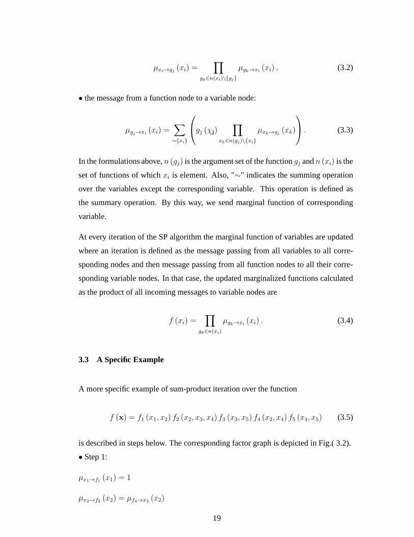
3.3 A Specific Example

A more specific example of sum-product iteration over the function

f (x) = f1 (x1, x2) f2 (x2, x3, x4) f3 (x3, x5) f4 (x2, x4) f5 (x4, x5) (3.5)

is described in steps below. The corresponding factor graphis depicted in Fig.( 3.2).

• Step 1:

µx1→f1 (x1) = 1

µx2→f2 (x2) = µf4→x2(x2)

19

x1 x2 x3 x4

f5f4f3f2f1

x5

µf1,x1

µx1,f1 µf1,x3

µx3,f1

Figure 3.2: A factor graph forf (x1, x2, x3, x4, x5)=f1 (x1, x3) f2 (x2, x3, x4) f3 (x3, x5) f4 (x2, x4) f5 (x4, x5)

µx2→f4 (x2) = µf2→x2(x2)

µx3→f1 (x3) = µf2→x3(x3)µf3→x3

(x3)

µx3→f2 (x3) = µf1→x3(x3)µf3→x3

(x3)

µx3→f3 (x3) = µf1→x3(x3)µf2→x3

(x3)

µx4→f2 (x4) = µf4→x4(x4)µf5→x4

(x4)

µx4→f4 (x4) = µf2→x4(x4)µf5→x4

(x4)

µx4→f5 (x4) = µf2→x4(x4)µf4→x4

(x4)

µx5→f3 (x5) = µf5→x5(x5)

µx5→f5 (x5) = µf3→x5(x5)

• Step 2:

µf1→x1(x1) =

∑∼{x1}

f1 (x1, x3)µx3→f1 (x3)

µf1→x3(x3) =

∑∼{x3}

f1 (x1, x3)µx1→f1 (x1)

µf2→x2(x2) =

∑∼{x2}

f2 (x2, x3, x4)µx3→f2 (x3)µx4→f2 (x4)

µf2→x3(x3, x4) =

∑∼{x3}

f2 (x2, x3)µx2→f2 (x2)µx4→f2 (x4)

µf2→x4(x4) =

∑∼{x4}

f2 (x2, x3x4)µx2→f2 (x2)µx3→f2 (x3)

20

µf3→x3(x3) =

∑∼{x3}

f3 (x3, x5)µx5→f3 (x5)

µf3→x5(x5) =

∑∼{x5}

f3 (x3, x5)µx3→f3 (x3)

µf4→x2(x2) =

∑∼{x2}

f4 (x2, x4)µx4→f4 (x4)

µf4→x4(x4) =

∑∼{x4}

f4 (x2, x4)µx2→f4 (x2)

µf5→x4(x4) =

∑∼{x4}

f5 (x4, x5)µx5→f5 (x5)

µf5→x5(x5) =

∑∼{x5}

f5 (x4, x5)µx4→f5 (x4)

Note that, since there is no message to variablex1, the message fromx1 to function

nodef1 is always 1. One iteration consists of these two steps. At theend of the

iteration, if one wants to calculate marginal function of the variables

f (x1) = µf1→x1(x1)

f (x2) = µf2→x2(x1)µf4→x2

(x2)

f (x3) = µf1→x3(x3)µf2→x3

(x3)µf3→x3(x3)

f (x4) = µf2→x4(x4)µf4→x4

(x4)µf5→x4(x4)

f (x5) = µf3→x5(x5)µf5→x5

(x5) .

In case of first iteration, all messages from a variable to a function node is unit mes-

sage, because we assume incoming messages to a variable nodewas unit message

[21]. After first iteration, all messages from variable nodes are executed as in step 1.

3.4 Soft-Input Soft-Output (SISO) Equalizer

Our one dimensional system model is based on linear modulations over linear chan-

nels affected by circularly symmetric complex white Gaussian noise. As a very gen-

eral form, the relationship between the transmitted sequencex = [x1, x2, ...., xN ]T

and the received sequencey = [y1, y2, ...., yN+L−1]T can be written as in [26]

y = Hx+w (3.6)

21

with

H =

h0 0 . . . . . . 0

... h0 0 . . . 0

hL−1 . . . h0...

0. . . . . .

.... .. . . . 0

hL−1 . . . h0

. . ....

0 . . . 0 hL−1

. (3.7)

wherew = [w1, w2, ...., wN+L−1]T are independent and identically distributed zero-

mean circularly symmetric complex Gaussian random variables, where real and imag-

inary parts are independent and have the same varianceσ2 = N0/2. The channel

convolutional matrixH hasK = N +L−1 rows andN columns whereL is channel

length.

In the equalization process, we want to compute MAP for symbols coming from finite

modulation given the observationy. To obtain MAP of the symbols individually, we

factor the pdf of (3.6) suitably according to [8].

3.4.1 Maximum A Posteriori (MAP) Detection of Symbols

The MAP detection of symbols requires calculating a posteriori probabilities (APP’s)

of p (xn | y) for all n and xn given the observationy. This task can be accom-

plished based onp (x | y) throughP (x), a priori probability of the sequence ofx,

andp (y | x), the conditional pdf ofy givenx.

Since we assume that there is no correlation between transmitted sequence symbols,

the probability of the sequence is written as

22

P (x) =N∏

n=1

Pn (xn) . (3.8)

The conditional pdf ofy given the transmitted sequencex equals

p (y | x) =(2πσ2

)−Kexp

(−‖ y −Hx ‖2

2σ2

). (3.9)

Since the factor(2πσ2)−K is independent of the transmitted sequencex, (3.9) can be

written with a proportionality factor, which indicates that two quantities are different

from each other by a constant factor independent ofx as given below

p (y | x) ∝ exp

(−‖ y −Hx ‖2

2σ2

). (3.10)

If we define

m = HHy (3.11)

S = HHH (3.12)

the norm square factor of (3.10) can be manipulated as

‖ y −Hx ‖2 = yHy− 2ℜ{xHHHy

}+ xHHHHx

=‖ y ‖2 −2ℜ{xHm

}+ xHSx. (3.13)

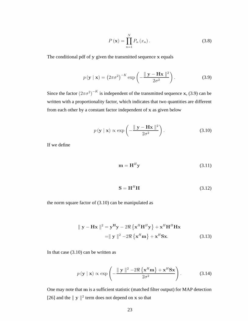
In that case (3.10) can be written as

p (y | x) ∝ exp

(−‖ y ‖2 −2ℜ

{xHm

}+ xHSx

2σ2

). (3.14)

One may note thatm is a sufficient statistic (matched filter output) for MAP detection

[26] and the‖ y ‖2 term does not depend onx so that

23

p (y | x) ∝ exp

(2ℜ{xHm

}− xHSx

2σ2

). (3.15)

3.4.2 Graph-Based Detection Algorithm

Factorization of a function can be performed in multiple ways. In [8], a specific

factorization was proposed to reduce the complexity of the sum-product algorithm to

scale linearly with the number of interfering signal terms.

Some manipulations should be made on the (3.15) to have a suitable factor graph for

SISO detection with SP algorithm. The scalar forms of matrixoperations in (3.15)

are

xHm =N∑

n=1

mnx∗n (3.16)

xHSx =

N∑

n=1

Sn,n | xn |2 +

N∑

n=1

N∑

k=1,k 6=n

x∗nSn,kxk

sinceSH = S,

xHSx =

N∑

n=1

Sn,n | xn |2 +

N∑

n=1

∑

k<n

2ℜ{x∗nSn,kxk} . (3.17)

By using these scalar forms, we can write the (3.15) as

p (y | x) =N∏

n=1

[exp

(1

σ2ℜ

{mnx

∗n −

Sn,n

2| xn |2

}) ∏

k<n

exp

(−

1

σ2ℜ{Sn,kxkx

∗n}

)].

(3.18)

In that case the function nodesTn (xn) andRn,k(xn,xk) are defined as

T (xn) = exp

(1

σ2ℜ

{mnx

∗n −

Sn,n

2| xn |2

}), (3.19)

24

Rn,k (xn, xk) = exp

[−

1

σ2ℜ{Sn,kxkx

∗n}

]. (3.20)

By using these definitions and a priori probabilities of the transmitted sequence, we

can factorize the APP density function

p (x | y) ∝ P (x) p (y | x) ∝N∏

n=1

[Pn (xn)Tn (xn)

∏

k<n

Rn,k (xn, xk)

](3.21)

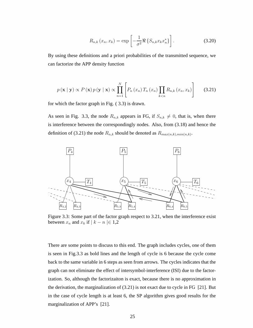
for which the factor graph in Fig. ( 3.3) is drawn.

As seen in Fig. 3.3, the nodeRn,k appears in FG, ifSn,k 6= 0, that is, when there

is interference between the correspondingly nodes. Also, from (3.18) and hence the

definition of (3.21) the nodeRn,k should be denoted asRmax(n,k),min(n,k).

P4

x4

R4,2

T4

P5

x5

R5,3

P6

x6

R6,5

T5 T6

R4,3 R5,4 R6,4

Figure 3.3: Some part of the factor graph respect to 3.21, when the interference existbetweenxn andxk if | k − n |∈ 1,2

There are some points to discuss to this end. The graph includes cycles, one of them

is seen in Fig.3.3 as bold lines and the length of cycle is 6 because the cycle come

back to the same variable in 6 steps as seen from arrows. The cycles indicates that the

graph can not eliminate the effect of intersymbol-interference (ISI) due to the factor-

ization. So, although the factorizaiton is exact, because there is no approximation in

the derivation, the marginalization of (3.21) is not exact due to cycle in FG [21]. But

in the case of cycle length is at least 6, the SP algorithm gives good results for the

marginalization of APP’s [21].

25

xk xn TnTk

Rn,k

µxn,Pnµxk,Pk

µRn,k,xk

µxk,Rn,k µxn,Rn,k

µRn,k,xn

PnPk

Figure 3.4: Propogated messages on the Factor Graph

By using the Fig.3.4, one can write marginalization of APPs as

p (xn | y) = Yn (xn) = Pn (xn) Tn (xn)∏

k 6=n

µRn,k→xn(xn) (3.22)

and the propagated messages

µxn→Pn(xn) =

Yn (xn)

Pn (xn)(3.23)

µxn→Rn,k(xn) =

Yn (xn)

µRn,k→xn(xn)

(3.24)

µRn,k→xn(xn) =

∑

xk

Rn,k (xn, xk)µxk→Rn,k(xk) . (3.25)

It is known from (3.5) the marginalization of a variable in a FG is product of all

incoming messages. HenceYn is marginalization ofp (x | y) respect toxn and so

p (xn | y). It is seen in (3.22) that the first two term are constant factor and the product

term is updating term which means thatµRn,k→xn(xn) bears APP information of node

k about noden. It can be inferred from (3.23) thatµxn→Pn(xn) is proportional to the

26

pdf p (y | xn) and it is produced by the algorithm as extrinsic informationto use

in turbo iteration process. Finally, it can be said that the nodeRn,k provides the

propagation of APPs between interfering variables after averaging operation.

Two of the computation methods which provide the marginal APPs from FG are

Parallel-Schedule Sum-Product algorithm (PS-SPA) and Serial-Schedule Sum-Product

algorithm (SS-SPA) [21]. In PS-SPA, same kind of messages are propagated at the

same time for all variables therefore it has feasibility forlow latency applications.

PS-SPA is implemented in the given order

1-) Update allYn terms,

2-) Update allµxn→Rn,kmessages,

3-) Update allµRn,k→xn messages,

4-) Go to step 1 in case of not satisfying the stopping criterion,

5-) Update allYn terms.

In SS-SPA, the message passings are executed first in forwarddirection from1 to

N after operation in the backward direction fromN to 1 for each variable node. The

forward recursion of SS-SPA for each value ofn from 1 to N is executed as given

below

1-) Update theµRn,k→xnmessages fork < n,

2-) Update theYn term ,

3-) Update theµxn→Rn,kmessages fork > n.

the backward recursion of SS-SPA can be executed for everyn from N to 1

27

1-) Update theµRn,k→xnmessages fork > n,

2-) Update theYn term,

3-) Update theµxn→Rn,kmessages fork < n,

and the SS-SPA is implemented through forward and backward recursion as in given

order

1-) Implement the forward recursion

2-) Implement the backward recursion

3-) Go to step 1 in case of not satisfying the stopping criterion.

Due to serial implementation of SS-SPAs, latency grows linearly with the valueN

hence it is feasible for applications where long operation time is not much of a prob-

lem.

Since the FG including cycles cannot eliminate ISI exactly and leads to overestima-

tion of reliability of messages propagated between nodes and factors [21]. Using

σ2 = N0/2 greater than actual one is suggested as a very basic trick to overcome this

problem in [8]. The rationale of the trick is to assume there is more noise than the

actual one and thereby to decrease the reliability of propagated messages. In simu-

lations, we use PS-SPA which is operated for one iteration. For relatively low SNR,

it is not required to useN0 greater than the actual one. For SNR values which10−3

packet error rate (PER) performance is achieved,N0 value should be generally chosen

slightly higher than the actulal one.

28

CHAPTER 4

CHANNEL ESTIMATION, TRACKING AND INTERLEAVER

DESIGN IN TIME DOMAIN

4.1 Introduction

Channel estimation is an important issue in wireless communication since provision

of communication reliability is usually contingent on the quality of channel state in-

formation. Channel estimation is usually made through pilot symbols between data

blocks. However, in fast fading channels, using only the pilots to estimate the chan-

nel may not be a solution of the issue since the coherence timemay be smaller than

data block duration. There are two solutions of this problem. One of them is to make

use of pilot symbol blocks more frequently in relation to thecoherence time, the other

one is to track the channel with some techniques such as Least-Mean-Squares (LMS),

Kalman filtering, Recursive-Least- Squares (RLS) etc. It isneeded to say that using

more pilots decreases throughput efficiency thereby is not preferred in many cases.

Therefore, the second solution is the suitable one for the problem in our case because

our interest is HF communication and the waveforms are givenin Military Standard

188110-C (ML-188110C). In this study, due to lower complexity and implementa-

tion feasibility, we prefer the LMS method to track the channel. By using suitable

interleaver with the channel tracking idea, channel tracking capability and the overall

performance are enhanced.

In this chapter, Firstly,the system model is illustrated. Secondly, the theoretical back-

ground of how the channel estimation is made through pilot symbols will be ex-

plained. Thirdly, the pilot extension idea is explained. Then, the uni-directional

29

LMS channel tracking and direct application to bidirectional channel tracking will be

asserted. In the interleaver design part, it is discussed why a new approach for the in-

terleaving process is required followed by proposing of a newly designed interleaver.

At the end, some corresponding results will be provided.

4.2 System Model for Receiver Part

LMS

Tracking

Interpolationand

EstimationChannel

Tracked

hn

LDe

LEe

Points

LD′

e

LE′

e

EstimatedPoints

yn

Interleaver

Deinterleaver

SISO SISObn : decoded

bits

DecoderEqualizer

Symbolto

LLR

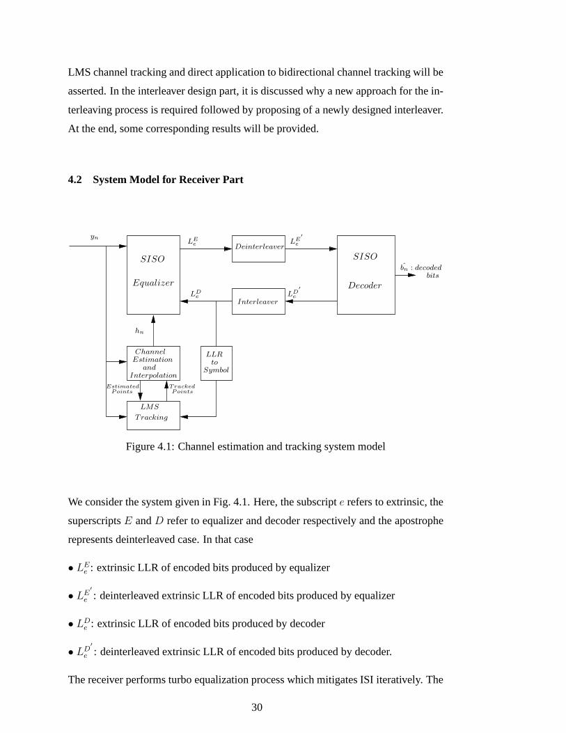
Figure 4.1: Channel estimation and tracking system model

We consider the system given in Fig. 4.1. Here, the subscripte refers to extrinsic, the

superscriptsE andD refer to equalizer and decoder respectively and the apostrophe

represents deinterleaved case. In that case

• LEe : extrinsic LLR of encoded bits produced by equalizer

• LE′

e : deinterleaved extrinsic LLR of encoded bits produced by equalizer

• LDe : extrinsic LLR of encoded bits produced by decoder

• LD′

e : deinterleaved extrinsic LLR of encoded bits produced by decoder.

The receiver performs turbo equalization process which mitigates ISI iteratively. The

30

proposed receiver performs iterative channel estimation through the following steps:

• Step 1: The channel is estimated at pilot blocks through Least Square (LS) estima-

tion method. In order to estimate the channel coefficients indata regions, the middle

points in the pilot regions are used in the interpolation process.

• Step 2: SISO equalizer performs equalization and producesLEe

• Step 3: Deinterleaving process is applied toLEe , thenLE

′

e is produced

• Step 4: The decoder performs decoding and producesLD′

e

• Step 5: Interleaving process is applied toLD′

e , thenLDe is produced

• Step 6: Extended pilot sequences are produced by LLR to symbol mapping

• Step 7: The channel is tracked up to borders of extended pilotblocks by the LMS

algorithm

• Step 8: Utilizing the middle points in the pilot region and the border points of the

extended pilot region, a new interpolation is executed.

• Step 9: The new channel estimates are used in the equalization process.

The above process continues from step 2 iteratively.

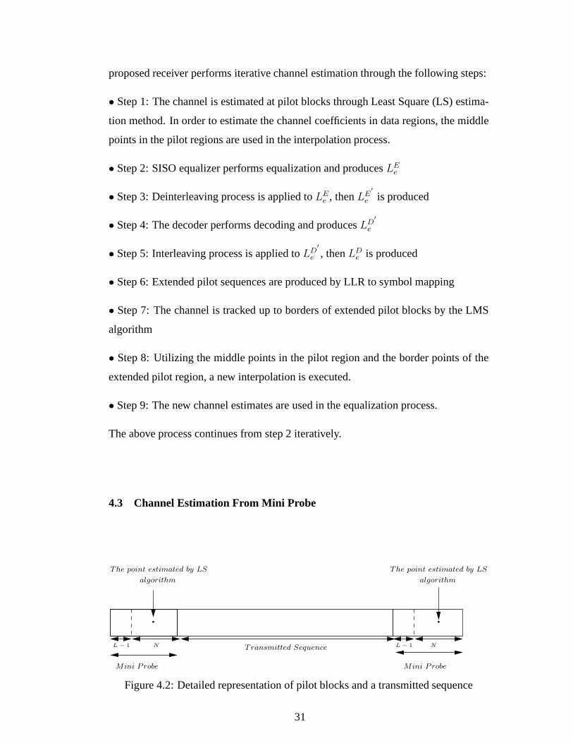
4.3 Channel Estimation From Mini Probe

Transmitted Sequence

. .

Mini Probe Mini Probe

NN

algorithm algorithm

L − 1L − 1

The point estimated by LSThe point estimated by LS

Figure 4.2: Detailed representation of pilot blocks and a transmitted sequence

31

The pilot blocks consist of multiple pilot symbols and referred to as mini probes in

this study. Under the assumption of a time-invariant channel, channel gain coeffi-

cients can be determined by observation of mini probes at thereceiver. If one wants

to estimate a channel withL taps, at leastL pilot symbols should be transmitted.

Channel estimation becomes better as there are more thanL pilot symbols in each

mini probe.

Consider a transmitted signalx = [x−L+1, ..., xN−1] in a mini probe. Since the first

L−1 observations are exposed to interference from data symbols, the received signals

after theseL − 1 observation are utilized in channel estimation. The observations

which are used in channel estimation

yn = sn + wn n = 0, . . . , N−1, (4.1)

wherewn denotes complex Gaussian noise sample andsn is given by

sn =

L−1∑

k=0

hkxn−k, n = 0, . . . , N−1. (4.2)

Then, we can write Eq. (4.1) in matrix form as

y = Xh+w , (4.3)

wherey = [y0, y1, ....., yN−1]T andh = [h0, h1, ....., hL−1]

T is channel.X is aN ×L

matrix with entries

[X]i+1,j+1 = xi−j 0 6 i 6 N − 1, 0 6 j 6 L− 1, (4.4)

and finallyw = [w0, w1, ..., wN−1] is a zero mean Gaussian vector with covariance

matrix

32

Cw = E[wwH

]= σ2

nIN. (4.5)

We define the signal-to-noise ratio SNR of the signal as

SNR =σ2s

σ2n

(4.6)

where

σ2s =

1

N

N−1∑

n=0

| s (n) |2 . (4.7)

We can now write the likelihood function ofy for givenh as given below:

p (y | h) =1

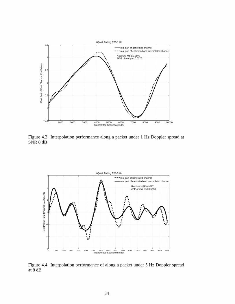
(πσ2n)

Nexp

{−

1

σ2n

[y−Xh]H [y −Xh]

}(4.8)

We will work with the Least Square (LS) estimate ofh which is given by [9] as

h =(XHX

)−1XHy. (4.9)

By applying this operation in all pilot regions individually, we can find the estimates

at approximately middle points of all pilot blocks as shown in Fig. 4.2. Then, inter-

polation provides channel estimates along the whole packet.

4.4 Extension of Pilot Blocks

Finding the channel coefficients between pilots by interpolation is reasonable for slow

varying channels. For instance, atFBW = 1 Hz, the channel coherence time is1

sec and the symbol duration is1/4800 ≈ 2 × 10−4 sec in the simulations. The time

33

0 1000 2000 3000 4000 5000 6000 7000 8000 9000 10000−0.5

0

0.5

1

1.5

2

2.54QAM, Fading BW=1 Hz

Transmitted Sequence Index

Rea

l Par

t of F

irst C

hann

el C

oeffi

cien

ts

real part of generated channelreal part of estimated and interpolated channel

Absolute MSE:0.0599MSE of real part:0.0276

Figure 4.3: Interpolation performance along a packet under1 Hz Doppler spread atSNR 8 dB

0 646 1258 1870 2482 3094 3706 4318 4930 5542 6154 6766 7378 7990 8602 9214 9826−3

−2

−1

0

1

2

34QAM, Fading BW=5 Hz

Transmitted Sequence Index

Rea

l Par

t of F

irst C

hann

el C

oeffi

cien

ts

real part of generated channelreal part of estimated and interpolated channel

Absolute MSE:0.9777MSE of real part:0.5333

Figure 4.4: Interpolation performance of along a packet under 5 Hz Doppler spreadat 8 dB

34

duration between pilot blocks is roughly 125 msecs. Hence , channel variation can

be tracked by interpolation by pilot blocks. However, the larger the fading bandwidth

is, the more the performance of interpolation diminishes. This is due to the fact that,

interpolation cannot track the channel under relatively fast time variation as observed

in Figures 4.3 and 4.4. Channel estimation such as in Fig. 4.4leads to error floor as

we will later observe in Section 4.5.

0 1088 2176 3264 4352 5440 6528 7616 8704 9792 10880 11968 13056 14144 15232 16320 17408−15

−10

−5

0

5

10

15

20

25

30

35

Encoded Bit Index of First Data Block

Tra

nsfo

rmed

LLR

val

ues

(dB

)

4QAM, FBW 5 Hz

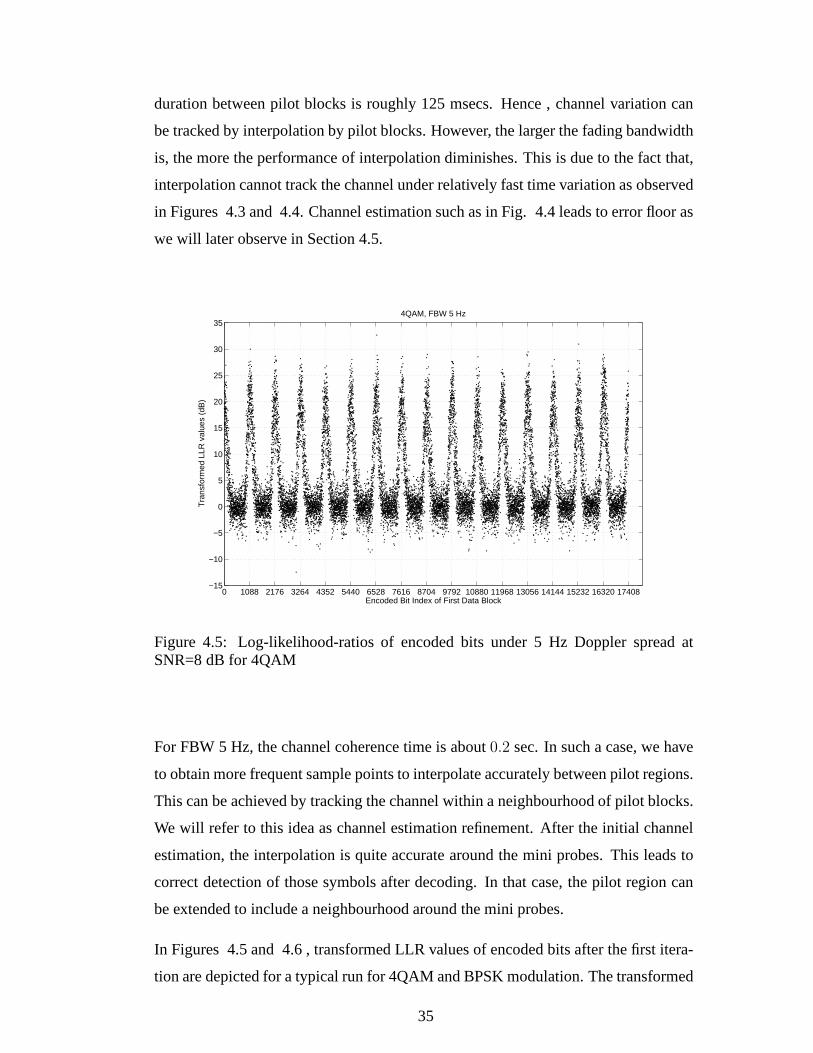
Figure 4.5: Log-likelihood-ratios of encoded bits under 5 Hz Doppler spread atSNR=8 dB for 4QAM

For FBW 5 Hz, the channel coherence time is about0.2 sec. In such a case, we have

to obtain more frequent sample points to interpolate accurately between pilot regions.

This can be achieved by tracking the channel within a neighbourhood of pilot blocks.

We will refer to this idea as channel estimation refinement. After the initial channel

estimation, the interpolation is quite accurate around themini probes. This leads to

correct detection of those symbols after decoding. In that case, the pilot region can

be extended to include a neighbourhood around the mini probes.

In Figures 4.5 and 4.6 , transformed LLR values of encoded bits after the first itera-

tion are depicted for a typical run for 4QAM and BPSK modulation. The transformed

35

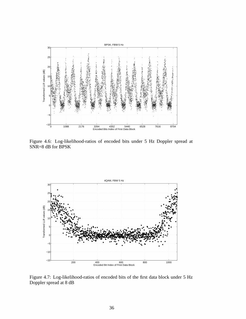
0 1088 2176 3264 4352 5440 6528 7616 8704−10

−5

0

5

10

15

20

25

30

Encoded Bits Index of First Data Block

Tra

nsfo

rmed

LLR

val

ues

(dB

)BPSK, FBW:5 Hz

Figure 4.6: Log-likelihood-ratios of encoded bits under 5 Hz Doppler spread atSNR=8 dB for BPSK

200 400 600 800 1000−15

−10

−5

0

5

10

15

20

25

30

Encoded Bit Index of First Data Block

Tra

nsfo

rmed

LLR

val

ues

(dB

)

4QAM, FBW 5 Hz

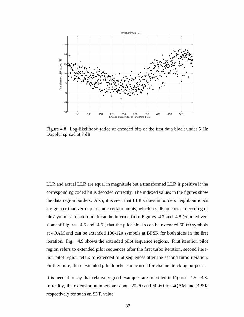
Figure 4.7: Log-likelihood-ratios of encoded bits of the first data block under 5 HzDoppler spread at 8 dB

36

50 100 150 200 250 300 350 400 450 500−10

−5

0

5

10

15

20

25

Encoded Bits Index of First Data Block

Tra

nsfo

rmed

LLR

val

ues

(dB

)

BPSK, FBW:5 Hz

Figure 4.8: Log-likelihood-ratios of encoded bits of the first data block under 5 HzDoppler spread at 8 dB

LLR and actual LLR are equal in magnitude but a transformed LLR is positive if the

corresponding coded bit is decoded correctly. The indexed values in the figures show

the data region borders. Also, it is seen that LLR values in borders neighbourhoods

are greater than zero up to some certain points, which results in correct decoding of

bits/symbols. In addition, it can be inferred from Figures 4.7 and 4.8 (zoomed ver-

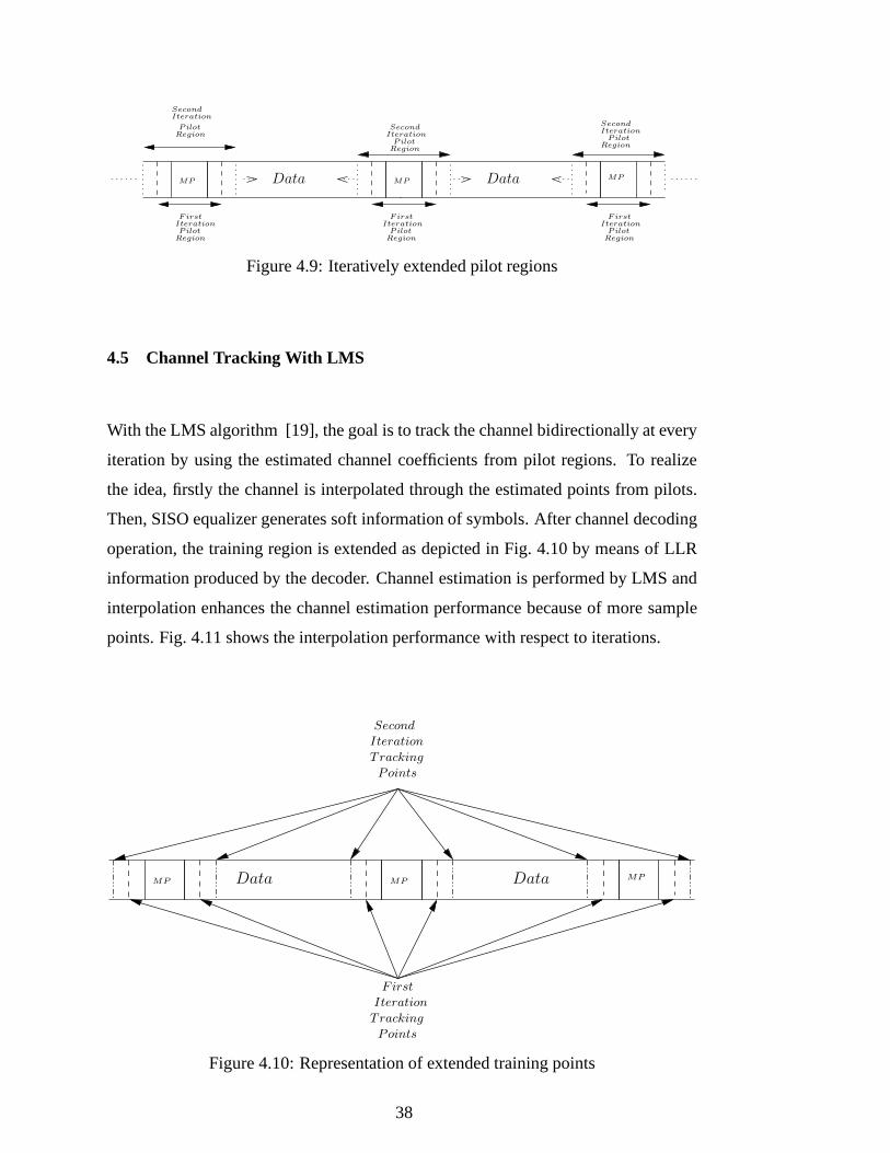
sions of Figures 4.5 and 4.6), that the pilot blocks can be extended 50-60 symbols

at 4QAM and can be extended 100-120 symbols at BPSK for both sides in the first

iteration. Fig. 4.9 shows the extended pilot sequence regions. First iteration pilot

region refers to extended pilot sequences after the first turbo iteration, second itera-

tion pilot region refers to extended pilot sequences after the second turbo iteration.

Furthermore, these extended pilot blocks can be used for channel tracking purposes.

It is needed to say that relatively good examples are provided in Figures 4.5- 4.8.

In reality, the extension numbers are about 20-30 and 50-60 for 4QAM and BPSK

respectively for such an SNR value.

37

MP MPMPDataData

Region

Second

PilotRegion

Pilot

Iteration

IterationFirst

PilotRegion

FirstIterationPilotRegion Region

FirstIterationPilot

SecondIterationPilot

Region

IterationSecond

Figure 4.9: Iteratively extended pilot regions

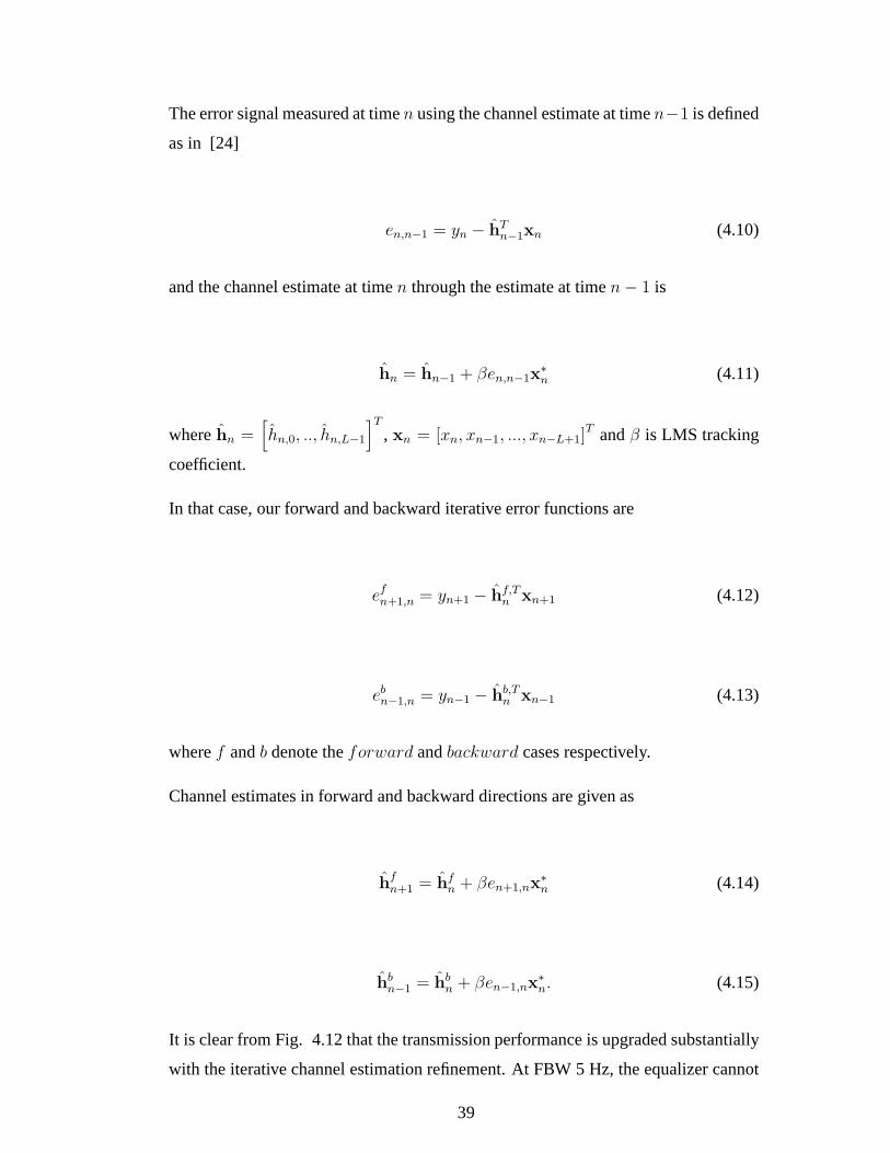
4.5 Channel Tracking With LMS

With the LMS algorithm [19], the goal is to track the channel bidirectionally at every

iteration by using the estimated channel coefficients from pilot regions. To realize

the idea, firstly the channel is interpolated through the estimated points from pilots.

Then, SISO equalizer generates soft information of symbols. After channel decoding

operation, the training region is extended as depicted in Fig. 4.10 by means of LLR

information produced by the decoder. Channel estimation isperformed by LMS and

interpolation enhances the channel estimation performance because of more sample

points. Fig. 4.11 shows the interpolation performance withrespect to iterations.

Data DataMP MPMP

Tracking

Points

T racking

Iteration

F irst

Second

Iteration

Points

Figure 4.10: Representation of extended training points

38

The error signal measured at timen using the channel estimate at timen−1 is defined

as in [24]

en,n−1 = yn − hTn−1xn (4.10)

and the channel estimate at timen through the estimate at timen− 1 is

hn = hn−1 + βen,n−1x∗n (4.11)

wherehn =[hn,0, .., hn,L−1

]T, xn = [xn, xn−1, ..., xn−L+1]

T andβ is LMS tracking

coefficient.

In that case, our forward and backward iterative error functions are

efn+1,n = yn+1 − hf,Tn xn+1 (4.12)

ebn−1,n = yn−1 − hb,Tn xn−1 (4.13)

wheref andb denote theforward andbackward cases respectively.

Channel estimates in forward and backward directions are given as

hfn+1 = hf

n + βen+1,nx∗n (4.14)

hbn−1 = hb

n + βen−1,nx∗n. (4.15)

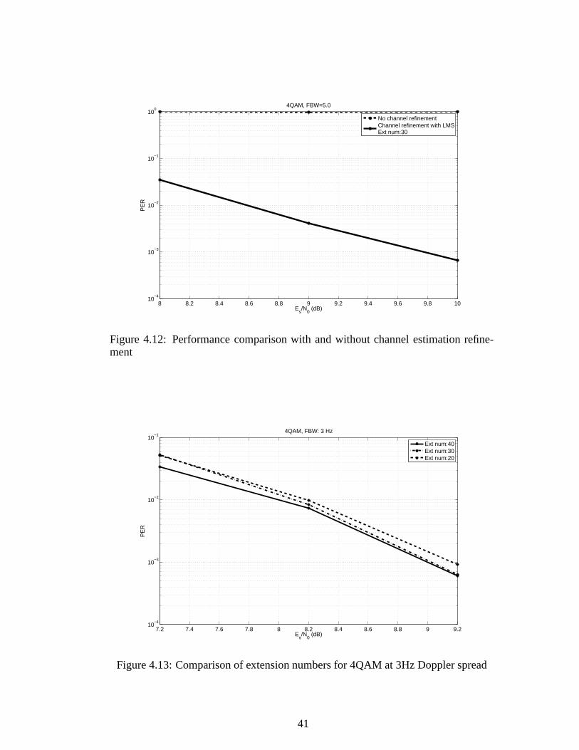
It is clear from Fig. 4.12 that the transmission performanceis upgraded substantially

with the iterative channel estimation refinement. At FBW 5 Hz, the equalizer cannot

39

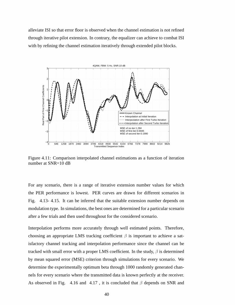
alleviate ISI so that error floor is observed when the channelestimation is not refined

through iterative pilot extension. In contrary, the equalizer can achieve to combat ISI

with by refining the channel estimation iteratively throughextended pilot blocks.

0 646 1258 1870 2482 3094 3706 4318 4930 5542 6154 6766 7378 7990 8602 9214 9826−4

−3

−2

−1

0

1

2

3

Transmitted Sequence Index

Rea

l Par

t of F

irst C

hann

el C

oeffi

cien

ts

4QAM, FBW: 5 Hz, SNR:10 dB

Known ChannelInterpolation at Initial IterationInterpeolation after First Turbo IterationInterpolation after Second Turbo Iteration

MSE of no iter:1.284MSE of first iter:0.6945MSE of second iter:0.1990

Figure 4.11: Comparison interpolated channel estimationsas a function of iterationnumber at SNR=10 dB

For any scenario, there is a range of iterative extension number values for which

the PER performance is lowest. PER curves are drawn for different scenarios in

Fig. 4.13- 4.15. It can be inferred that the suitable extension number depends on

modulation type. In simulations, the best ones are determined for a particular scenario

after a few trials and then used throughout for the considered scenario.

Interpolation performs more accurately through well estimated points. Therefore,

choosing an appropriate LMS tracking coefficientβ is important to achieve a sat-

isfactory channel tracking and interpolation performancesince the channel can be

tracked with small error with a proper LMS coefficient. In thestudy,β is determined

by mean squared error (MSE) criterion through simulations for every scenario. We

determine the experimentally optimum beta through 1000 randomly generated chan-

nels for every scenario where the transmitted data is known perfectly at the receiver.

As observed in Fig. 4.16 and 4.17 , it is concluded thatβ depends on SNR and

40

8 8.2 8.4 8.6 8.8 9 9.2 9.4 9.6 9.8 1010

−4

10−3

10−2

10−1

100

PE

R

Es/N

0 (dB)

4QAM, FBW=5.0

No channel refinementChannel refinement with LMSExt num:30

Figure 4.12: Performance comparison with and without channel estimation refine-ment

7.2 7.4 7.6 7.8 8 8.2 8.4 8.6 8.8 9 9.210

−4

10−3

10−2

10−1

PE

R

Es/N

0 (dB)

4QAM, FBW: 3 Hz

Ext num:40Ext num:30Ext num:20

Figure 4.13: Comparison of extension numbers for 4QAM at 3HzDoppler spread

41

8 8.2 8.4 8.6 8.8 9 9.2 9.4 9.6 9.8 1010

−4

10−3

10−2

10−1

100

PE

R

Es/N

0 (dB)

4QAM, FBW: 5 Hz

Ext num:30Ext num:20Ext num 10

Figure 4.14: Comparison of extension numbers for 4QAM at 5HzDoppler spread

4 4.2 4.4 4.6 4.8 5 5.2 5.4 5.6 5.8 610

−4

10−3

10−2

10−1

PE

R

Es/N

0 (dB)

4QAM, FBW: 5 Hz

Ext num:70Ext num:60Ext num:50

Figure 4.15: Comparison of extension numbers for BPSK at 5HzDoppler spread

42

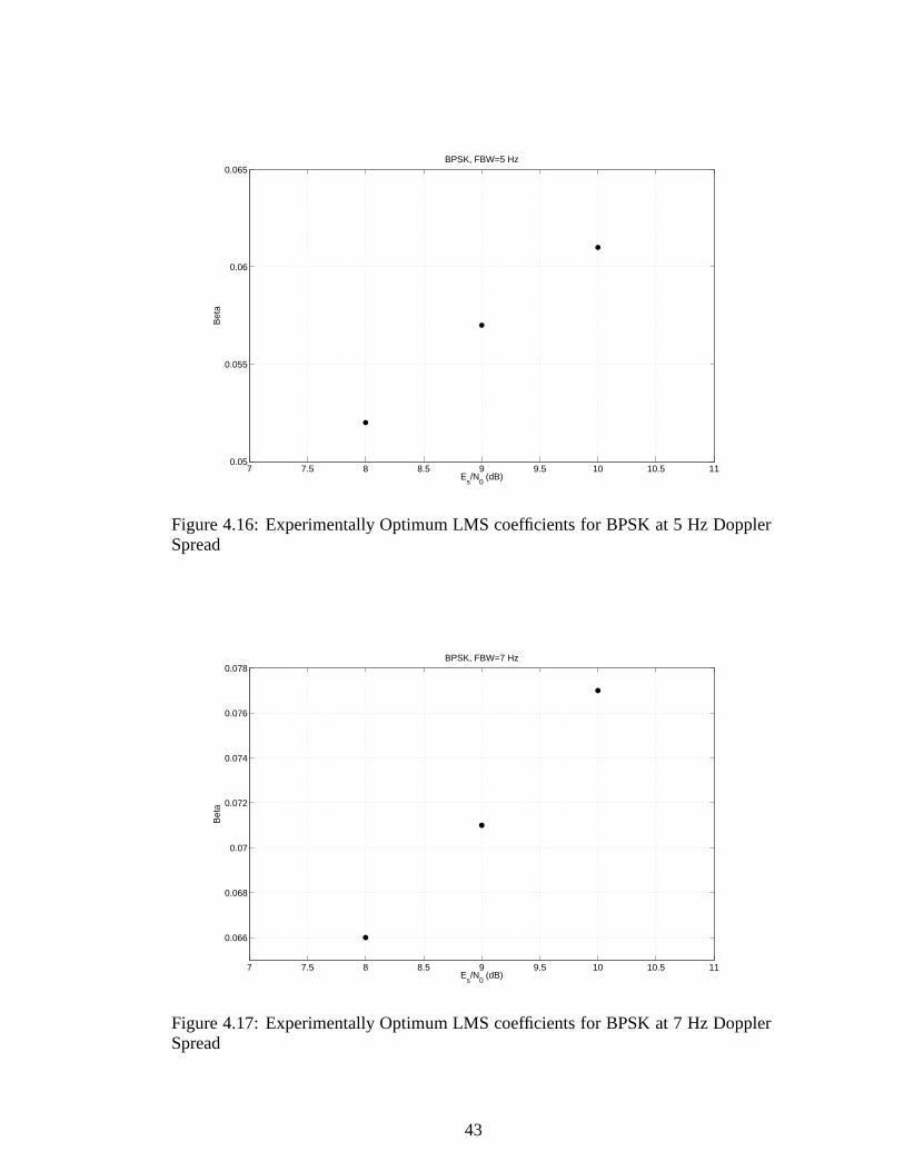
7 7.5 8 8.5 9 9.5 10 10.5 110.05

0.055

0.06

0.065

Bet

a

Es/N

0 (dB)

BPSK, FBW=5 Hz

Figure 4.16: Experimentally Optimum LMS coefficients for BPSK at 5 Hz DopplerSpread

7 7.5 8 8.5 9 9.5 10 10.5 11

0.066

0.068

0.07

0.072

0.074

0.076

0.078

Bet

a

Es/N

0 (dB)

BPSK, FBW=7 Hz

Figure 4.17: Experimentally Optimum LMS coefficients for BPSK at 7 Hz DopplerSpread

43

fading bandwidth.

100 200 300 400 500 600 700 800 900 1000

−5

0

5

10

15

Symbol index of first transmitted data block

Tra

nsfo

rmed

ext

rinsi

c LL

R o

f Equ

aliz

er

4QAM, FBw:5 Hz

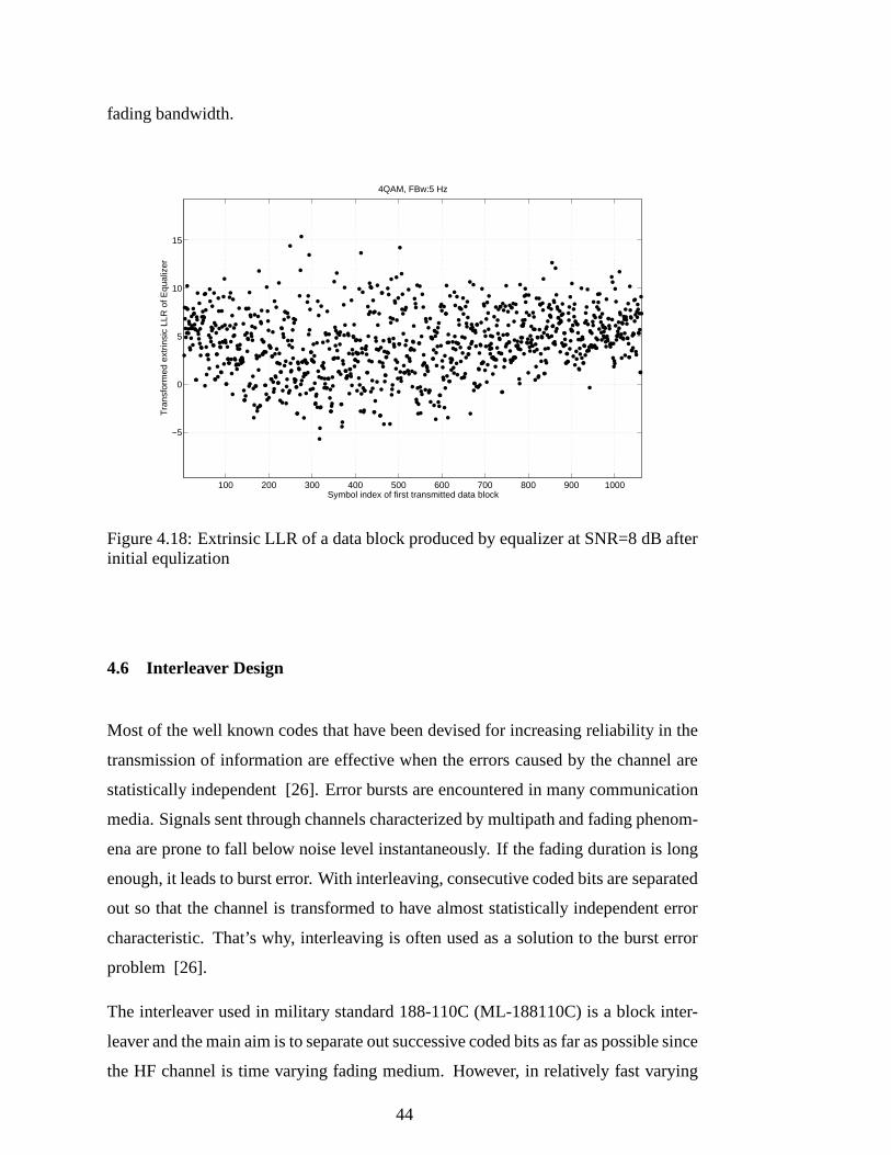
Figure 4.18: Extrinsic LLR of a data block produced by equalizer at SNR=8 dB afterinitial equlization

4.6 Interleaver Design

Most of the well known codes that have been devised for increasing reliability in the

transmission of information are effective when the errors caused by the channel are

statistically independent [26]. Error bursts are encountered in many communication

media. Signals sent through channels characterized by multipath and fading phenom-

ena are prone to fall below noise level instantaneously. If the fading duration is long

enough, it leads to burst error. With interleaving, consecutive coded bits are separated

out so that the channel is transformed to have almost statistically independent error

characteristic. That’s why, interleaving is often used as asolution to the burst error

problem [26].

The interleaver used in military standard 188-110C (ML-188110C) is a block inter-

leaver and the main aim is to separate out successive coded bits as far as possible since

the HF channel is time varying fading medium. However, in relatively fast varying

44

0 100 200 300 400 500 600 700 800 900 1000

−5

0

5

10

15

20

25

Symbol index of first transmitted data block

Tra

nsfo

rmed

ext

rinsi

c LL

R o

f dec

oder

4QAM, FBW:5 Hz

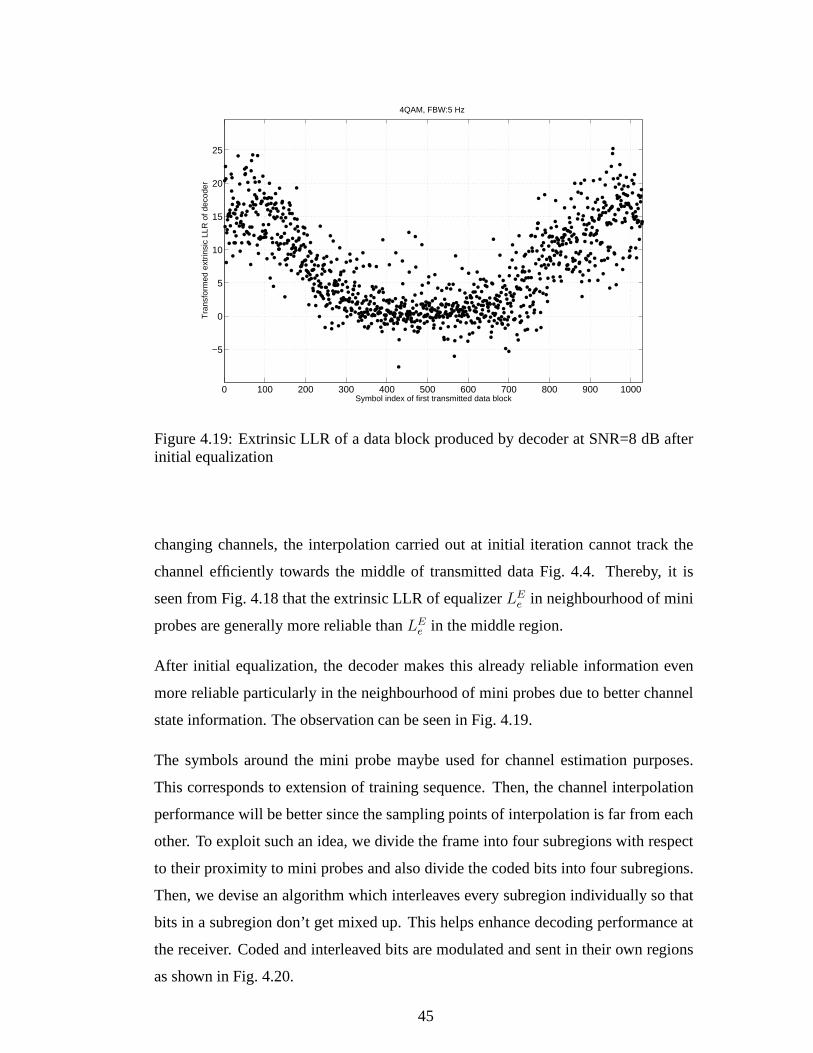
Figure 4.19: Extrinsic LLR of a data block produced by decoder at SNR=8 dB afterinitial equalization

changing channels, the interpolation carried out at initial iteration cannot track the

channel efficiently towards the middle of transmitted data Fig. 4.4. Thereby, it is

seen from Fig. 4.18 that the extrinsic LLR of equalizerLEe in neighbourhood of mini

probes are generally more reliable thanLEe in the middle region.

After initial equalization, the decoder makes this alreadyreliable information even

more reliable particularly in the neighbourhood of mini probes due to better channel

state information. The observation can be seen in Fig. 4.19.

The symbols around the mini probe maybe used for channel estimation purposes.

This corresponds to extension of training sequence. Then, the channel interpolation

performance will be better since the sampling points of interpolation is far from each

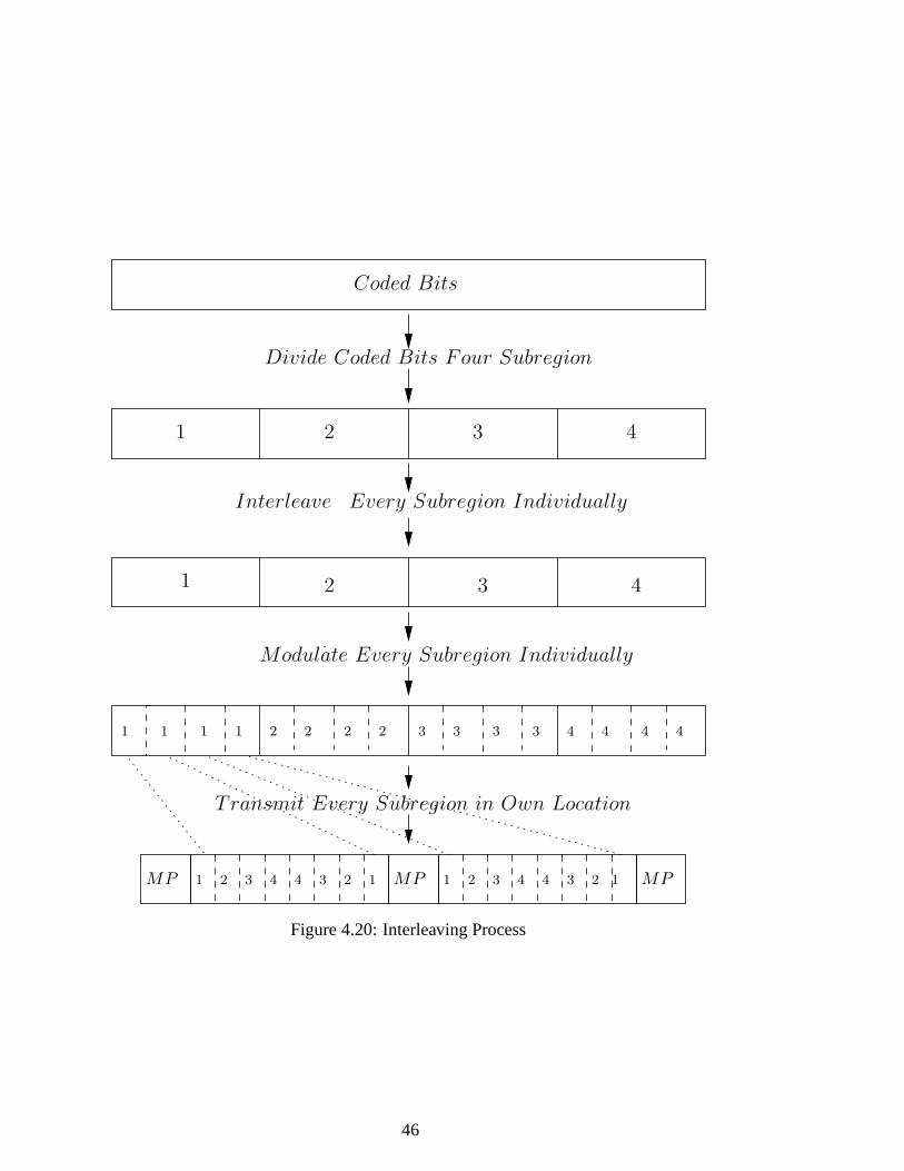
other. To exploit such an idea, we divide the frame into four subregions with respect

to their proximity to mini probes and also divide the coded bits into four subregions.

Then, we devise an algorithm which interleaves every subregion individually so that

bits in a subregion don’t get mixed up. This helps enhance decoding performance at

the receiver. Coded and interleaved bits are modulated and sent in their own regions

as shown in Fig. 4.20.

45

MP MP MP

1 2 3 4

1 2 3 4

1 1 1 1 2 2 2 2 3 3 3 3 4 4 4 4

1 2 3 4 4 3 2 1 1 2 3 4 4 3 2 1

Every Subregion Individually

Modulate Every Subregion Individually

Coded Bits

Divide Coded Bits Four Subregion

Interleave

Transmit Every Subregion in Own Location

Figure 4.20: Interleaving Process

46

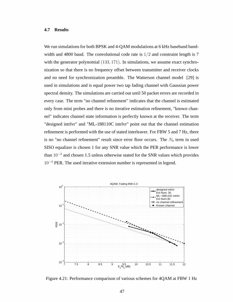
4.7 Results

We run simulations for both BPSK and 4-QAM modulations at 6 kHz baseband band-

width and 4800 baud. The convolutional code rate is1/2 and constraint length is 7

with the generator polynomial(133, 171). In simulations, we assume exact synchro-

nization so that there is no frequency offset between transmitter and receiver clocks

and no need for synchronization preamble. The Watterson channel model [29] is

used in simulations and is equal power two tap fading channelwith Gaussian power

spectral density. The simulations are carried out until 50 packet errors are recorded in

every case. The term "no channel refinement" indicates that the channel is estimated

only from mini probes and there is no iterative estimation refinement, "known chan-

nel" indicates channel state information is perfectly known at the receiver. The term

"designed intrlvr" and "ML-188110C intrlvr" point out thatthe channel estimation

refinement is performed with the use of stated interleaver. For FBW 5 and 7 Hz, there

is no "no channel refinement" result since error floor occurs.TheN0 term in used

SISO equalizer is chosen 1 for any SNR value which the PER performance is lower

than10−3 and chosen 1.5 unless otherwise stated for the SNR values which provides

10−3 PER. The used iterative extension number is represented in legend.

7 7.5 8 8.5 9 9.5 10 10.5 11 11.5 1210

−4

10−3

10−2

10−1

100

PE

R

Es/N

0 (dB)

4QAM, Fading BW=1.0

designed intrlvrExt Num: 30ML−188110C intrlvrExt Num:30no channel refinementKnown channel

Figure 4.21: Performance comparison of various schemes for4QAM at FBW 1 Hz

47

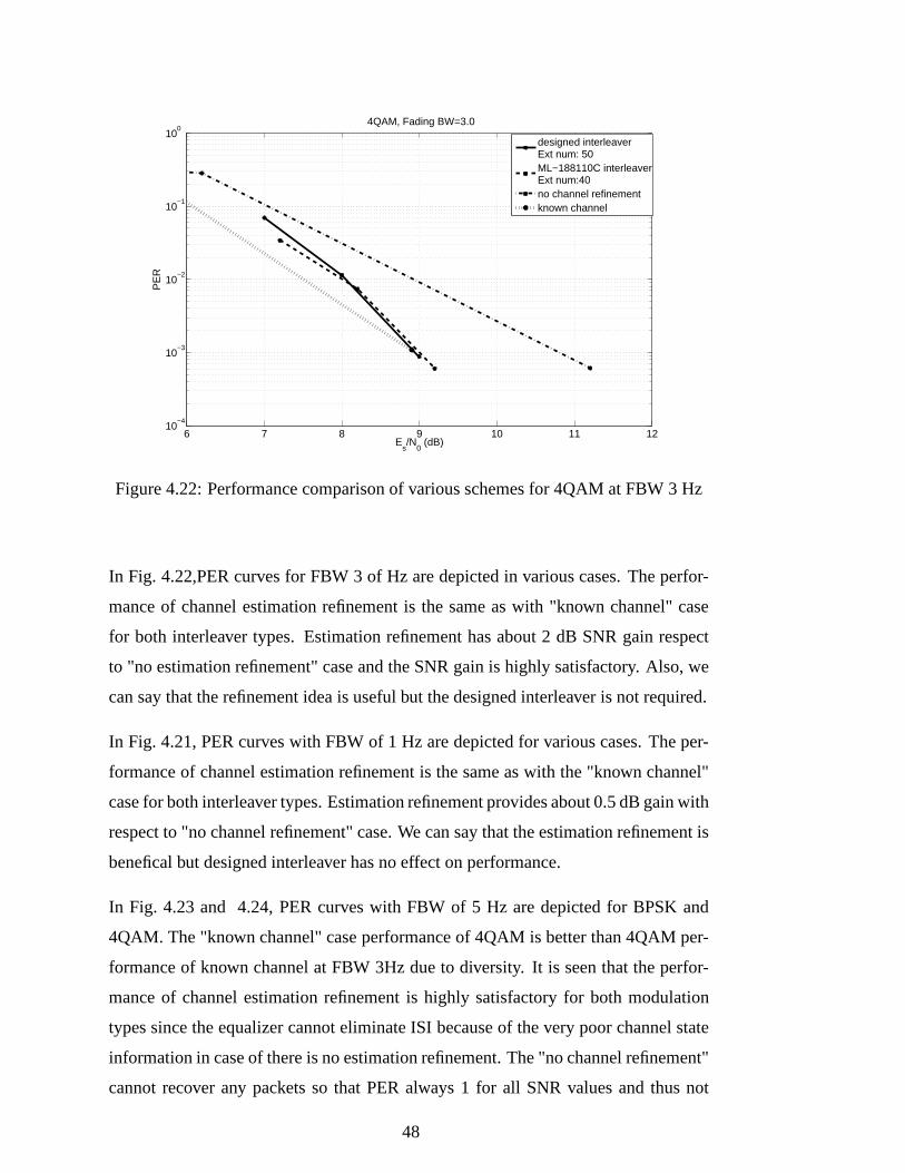
6 7 8 9 10 11 1210

−4

10−3

10−2

10−1

100

PE

R

Es/N

0 (dB)

4QAM, Fading BW=3.0

designed interleaverExt num: 50ML−188110C interleaverExt num:40no channel refinementknown channel

Figure 4.22: Performance comparison of various schemes for4QAM at FBW 3 Hz

In Fig. 4.22,PER curves for FBW 3 of Hz are depicted in variouscases. The perfor-

mance of channel estimation refinement is the same as with "known channel" case

for both interleaver types. Estimation refinement has about2 dB SNR gain respect

to "no estimation refinement" case and the SNR gain is highly satisfactory. Also, we

can say that the refinement idea is useful but the designed interleaver is not required.

In Fig. 4.21, PER curves with FBW of 1 Hz are depicted for various cases. The per-

formance of channel estimation refinement is the same as withthe "known channel"

case for both interleaver types. Estimation refinement provides about 0.5 dB gain with

respect to "no channel refinement" case. We can say that the estimation refinement is

benefical but designed interleaver has no effect on performance.

In Fig. 4.23 and 4.24, PER curves with FBW of 5 Hz are depicted for BPSK and

4QAM. The "known channel" case performance of 4QAM is betterthan 4QAM per-

formance of known channel at FBW 3Hz due to diversity. It is seen that the perfor-

mance of channel estimation refinement is highly satisfactory for both modulation

types since the equalizer cannot eliminate ISI because of the very poor channel state

information in case of there is no estimation refinement. The"no channel refinement"

cannot recover any packets so that PER always 1 for all SNR values and thus not

48

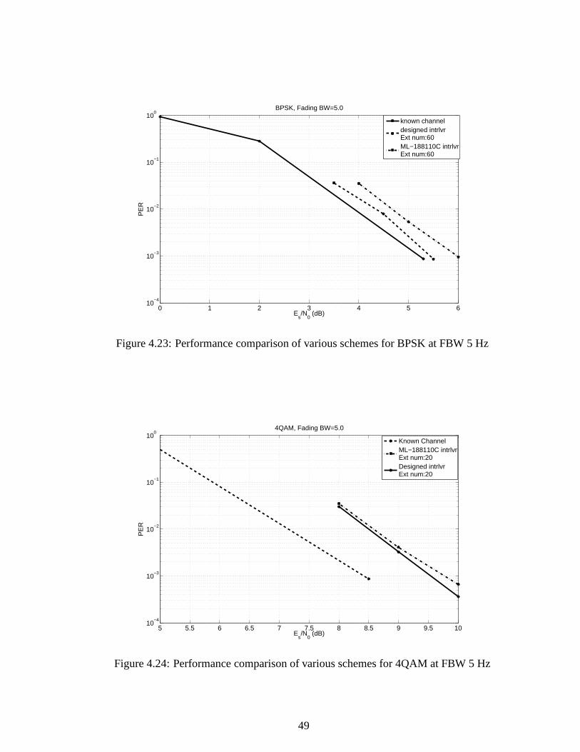
0 1 2 3 4 5 610

−4

10−3

10−2

10−1

100

PE

R

Es/N

0 (dB)

BPSK, Fading BW=5.0

known channeldesigned intrlvrExt num:60ML−188110C intrlvrExt num:60

Figure 4.23: Performance comparison of various schemes forBPSK at FBW 5 Hz

5 5.5 6 6.5 7 7.5 8 8.5 9 9.5 1010

−4

10−3

10−2

10−1

100

PE

R

Es/N

0 (dB)

4QAM, Fading BW=5.0

Known ChannelML−188110C intrlvrExt num:20Designed intrlvrExt num:20

Figure 4.24: Performance comparison of various schemes for4QAM at FBW 5 Hz

49

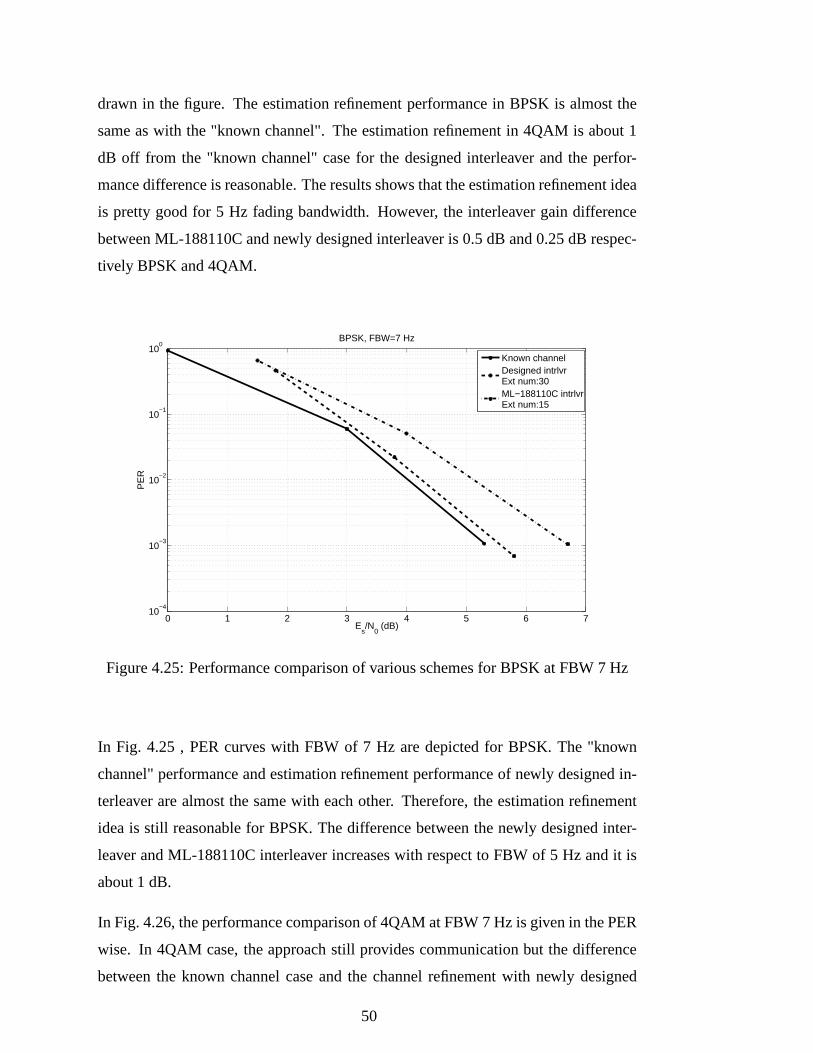
drawn in the figure. The estimation refinement performance inBPSK is almost the

same as with the "known channel". The estimation refinement in 4QAM is about 1

dB off from the "known channel" case for the designed interleaver and the perfor-

mance difference is reasonable. The results shows that the estimation refinement idea

is pretty good for 5 Hz fading bandwidth. However, the interleaver gain difference

between ML-188110C and newly designed interleaver is 0.5 dBand 0.25 dB respec-

tively BPSK and 4QAM.

0 1 2 3 4 5 6 710

−4

10−3

10−2

10−1

100

PE

R

Es/N

0 (dB)

BPSK, FBW=7 Hz

Known channelDesigned intrlvrExt num:30ML−188110C intrlvrExt num:15

Figure 4.25: Performance comparison of various schemes forBPSK at FBW 7 Hz

In Fig. 4.25 , PER curves with FBW of 7 Hz are depicted for BPSK.The "known

channel" performance and estimation refinement performance of newly designed in-

terleaver are almost the same with each other. Therefore, the estimation refinement

idea is still reasonable for BPSK. The difference between the newly designed inter-

leaver and ML-188110C interleaver increases with respect to FBW of 5 Hz and it is

about 1 dB.

In Fig. 4.26, the performance comparison of 4QAM at FBW 7 Hz isgiven in the PER

wise. In 4QAM case, the approach still provides communication but the difference

between the known channel case and the channel refinement with newly designed

50

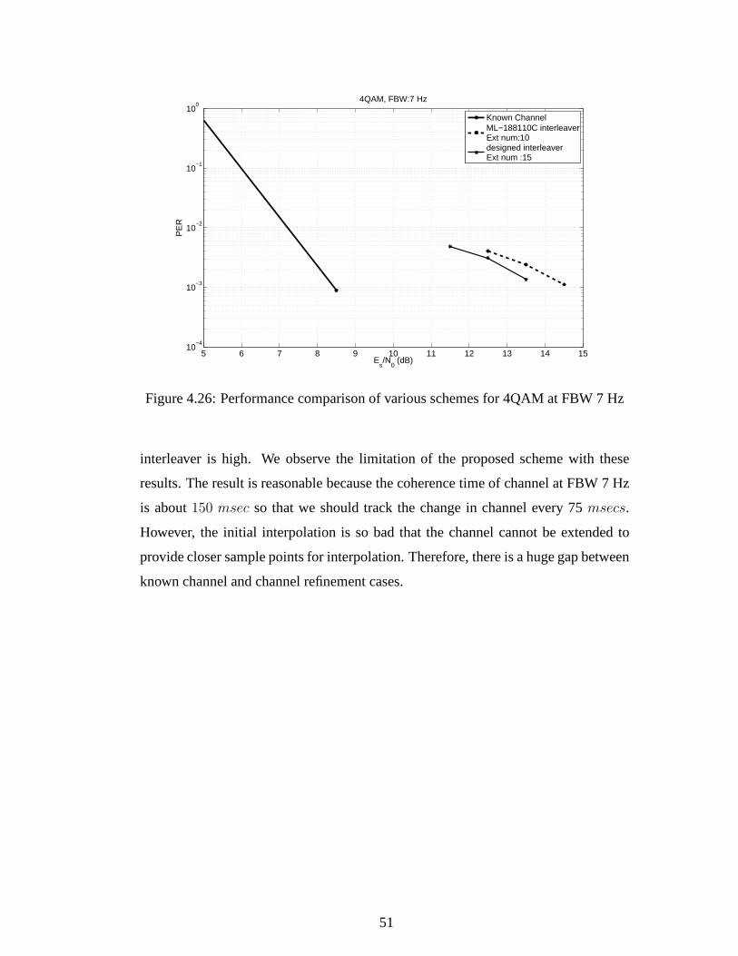
5 6 7 8 9 10 11 12 13 14 1510

−4

10−3

10−2

10−1

100

PE

R

Es/N

0 (dB)

4QAM, FBW:7 Hz

Known ChannelML−188110C interleaverExt num:10designed interleaverExt num :15

Figure 4.26: Performance comparison of various schemes for4QAM at FBW 7 Hz

interleaver is high. We observe the limitation of the proposed scheme with these

results. The result is reasonable because the coherence time of channel at FBW 7 Hz

is about150 msec so that we should track the change in channel every 75msecs.

However, the initial interpolation is so bad that the channel cannot be extended to

provide closer sample points for interpolation. Therefore, there is a huge gap between

known channel and channel refinement cases.

51

52

CHAPTER 5

CONCLUSION

In wireless communication, the bearing electromagnetic waves interact with the sur-

rounding medium which results in multipath signals. Movements of the transmitter

or receiver leads to time variation in received signal power. Therefore, the wireless

communication channel is characterized by ISI and fading. To provide good commu-

nication quality, channel estimation is necessary and is anintegral part of the receiver

since the equalizer can eliminate ISI with channel state information. Therefore, pilot

sequences which are known by transmitter and receiver are utilized for channel esti-

mation in many communication environment with some period.However, the pilot

sequence is not a solution of the channel estimation problemin fast fading chan-

nels since the interpolation used with the channel estimation cannot track the channel

properly. As a solution of such a problem, we propose to extend the training se-

quences by the aid of soft information produced by the channel decoder and to track

the channel through the extended sequences to provide better interpolation. In addi-

tion, the interpolation performance at initial iteration is better at the neighbourhood

of pilot sequences. Therefore, an interleaver which makes use of the better estimated

region of the channel enhances the interpolation performance since it provides longer

extended sequence.

As a result, the main contribution of this dissertation is given below:

• With channel tracking operated bidirectionally with LMS through the extended

training sequences, interpolation capability is increased resulting equalizer perfor-

mance enhancement.

53

• We subdivide the coded bits into subregions and interleave every subregion individ-

ually then send the transmitted symbols in their corresponding channel regions. With

this application the chanel tracking capability is sometimes enhanced.

Possible future works are

• Channel tracking can be applied to OFDM transmission to estimate the channel

both in time and frequency domains,

• By designing a two dimensional interleaver regarding the pilot inserting regime in

the OFDM frame, the throughput as well as channel estimationand tracking perfor-

mance can be enhanced.

•Performance of the proposed scheme can be investigated by using other SISO equal-

izers.

•Performance of the proposed scheme can be investigated by using the channel statis-

tics in interpolation.

54

REFERENCES

[1] A. W. A. Oppenheim.Signals and Systems. Prentice Hall, 1997.

[2] G. E. B. Arslan Hüseyin. Channel estimation in narrowband wireless commu-nication systems.Wirel. Commun. Mob. Comput., pages 201–219, 2001.

[3] M. Austin, A. Buckley, C. Coursey, P. Hartman, R. Kobylinski, M. Majmundar,K. Raith, and J. Seymour. Service and system enhancements for tdma digitalcellular systems.Personal Communications, IEEE, 6(3):20–33, Jun 1999.

[4] G. Bauch, H. Khorram, and J. Hagenauer. Iterative equalization and decodingin mobile communications systems. pages 307–312, 1997.

[5] G. Bottomley and S. Chennakeshu. Unification of mlse receivers and extensionto time-varying channels.Communications, IEEE Transactions on, 46(4):464–472, Apr 1998.

[6] G. Bottomley and S. Chennakeshu. Unification of mlse receivers and extensionto time-varying channels.Communications, IEEE Transactions on, 46(4):464–472, Apr 1998.

[7] J. Cavers. An analysis of pilot symbol assisted modulation for rayleigh fad-ing channels [mobile radio]. Vehicular Technology, IEEE Transactions on,40(4):686–693, Nov 1991.

[8] G. Colavolpe, D. Fertonani, and A. Piemontese. SISO detection over linearchannels with linear complexity in the number of interferers. Selected Topics inSignal Processing, IEEE Journal of, 5(8):1475–1485, Dec 2011.

[9] S. Crozier, D. Falconer, and S. Mahmoud. Least sum of squared errors(lsse) channel estimation.Radar and Signal Processing, IEE Proceedings F,138(4):371–378, Aug 1991.

[10] P. V. David Tse.Fundamentals of Wireless communications. Cambridge Uni-versity Press, - edition, 2005.

[11] E. de Carvalho and D. T. M. Slock. Blind and semi-blind firmultichannel es-timation: (global) identifiability conditions.Signal Processing, IEEE Transac-tions on, 52(4):1053–1064, April 2004.

[12] C. Douillard, M. Jézéquel, C. Berrou, D. Electronique,A. Picart, P. Didier,and A. Glavieux. Iterative correction of intersymbol interference: Turbo-equalization.European Transactions on Telecommunications, pages 507–511,1995.

[13] Giles. On the Design of HF Radio Modems. Ph.d. dissertation, The Universityof Adelaide, Australia, 1995.

55

[14] A. Goldsmith. Wireless communications. Cambridge University Press, fifthedition, 2005.

[15] D. Goodman. Second generation wireless information networks. VehicularTechnology, IEEE Transactions on, 40(2):366–374, May 1991.

[16] D. Goodman. Second generation wireless information networks. VehicularTechnology, IEEE Transactions on, 40(2):366–374, May 1991.

[17] J. M. Goodman.HF Communications. Science and Technology. Van NostrandReinhold, 1992.

[18] B. L. W. Hall, M. P. M. and Hewitt.Propagation of Radio Waves. The Institu-tion of Electrical Engineers, 1996.

[19] M. H. Hayes. Statistical Digital Signal Processing and Modeling. J. Wiley,1996.

[20] D. K. Ionospheric Radio. Peter Peregrinus Ltd., 1990.

[21] F. Kschischang, B. Frey, and H.-A. Loeliger. Factor graphs and the sum-productalgorithm. Information Theory, IEEE Transactions on, 47(2):498–519, Feb2001.

[22] R. W. E. Mcnicol. The fading of radio waves of medium and high frequen-cies.Proceedings of the IEE - Part III: Radio and Communication Engineering,96(44):517–524, November 1949.

[23] R. Otnes.Improved Receivers for Digital High Frequency Coomunications: It-erative Channel Estimation and Decoding (Adaptive Turbo Equalization). Ph.d.dissertation, Dept. of Telecommunications, Norwegian University of Scienceand Technology, Norway, 2002.

[24] R. Otnes and M. Tüchler. Iterative channel estimation for turbo equalizationof time-varying frequency-selective channels.Wireless Communications, IEEETransactions on, 3(6):1918–1923, Nov 2004.

[25] R. Otnes and M. Tüchler. Iterative channel estimation for turbo equalizationof time-varying frequency-selective channels.Wireless Communications, IEEETransactions on, 3(6):1918–1923, Nov 2004.

[26] J. Proakis and M. Salehi.Digital communications. McGraw-Hill Education,fifth edition, 2007.

[27] S. Song, A. Singer, and K.-M. Sung. Soft input channel estimation for turboequalization.Signal Processing, IEEE Transactions on, 52(10):2885–2894, Oct2004.

[28] J. Tugnait, L. Tong, and Z. Ding. Single-user channel estimation and equaliza-tion. Signal Processing Magazine, IEEE, 17(3):16–28, May 2000.

[29] C. Watterson, J. Juroshek, and W. Bensema. Experimental confirmation of an hfchannel model.Communication Technology, IEEE Transactions on, 18(6):792–803, December 1970.

56

[30] J. Wu and A. Aghvami. A new adaptive equalizer with a channel estimatorfor mobile radio communications. InCommunications, 1995. ICC ’95 Seattle,’Gateway to Globalization’, 1995 IEEE International Conference on, volume 2,pages 998–1002 vol.2, Jun 1995.

[31] R. Ziegler, M. Al-Dhahir, and J. Cioffi. Nonrecursive adaptive decision-feedback equalization from channel estimates. InVehicular Technology Con-ference, 1992, IEEE 42nd, pages 600–603 vol.2, May 1992.

57