Embed Size (px)
Citation preview
Linear RegressionPoisson Regression
Beyond Poisson Regression
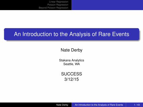
An Introduction to the Analysis of Rare Events
Nate Derby
Stakana AnalyticsSeattle, WA
SUCCESS3/12/15
Nate Derby An Introduction to the Analysis of Rare Events 1 / 43
Linear RegressionPoisson Regression
Beyond Poisson Regression
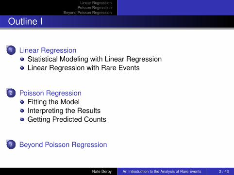
Outline I
1 Linear RegressionStatistical Modeling with Linear RegressionLinear Regression with Rare Events
2 Poisson RegressionFitting the ModelInterpreting the ResultsGetting Predicted Counts
3 Beyond Poisson Regression
Nate Derby An Introduction to the Analysis of Rare Events 2 / 43
Linear RegressionPoisson Regression
Beyond Poisson Regression
Statistical Modeling with Linear RegressionLinear Regression with Rare Events
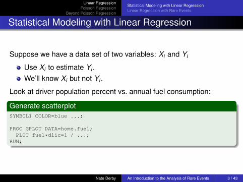
Statistical Modeling with Linear Regression
Suppose we have a data set of two variables: Xi and Yi
Use Xi to estimate Yi .We’ll know Xi but not Yi .
Look at driver population percent vs. annual fuel consumption:
Generate scatterplotSYMBOL1 COLOR=blue ...;
PROC GPLOT DATA=home.fuel;PLOT fuel*dlic=1 / ...;
RUN;
Nate Derby An Introduction to the Analysis of Rare Events 3 / 43

Linear RegressionPoisson Regression
Beyond Poisson Regression
Statistical Modeling with Linear RegressionLinear Regression with Rare Events
Ann
ual F
uel C
onsu
mpt
ion
per
Pers
on (
x 10
00 g
allo
ns)
30
50
70
90
Driver Population Percentage
70% 80% 90% 100% 110%
Fuel Consumption vs Driver Population PercentageScatterplot
Nate Derby An Introduction to the Analysis of Rare Events 4 / 43
Linear RegressionPoisson Regression
Beyond Poisson Regression
Statistical Modeling with Linear RegressionLinear Regression with Rare Events
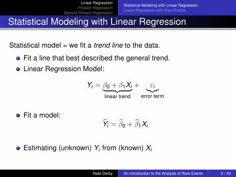
Statistical Modeling with Linear Regression
Statistical model = we fit a trend line to the data.
Fit a line that best described the general trend.Linear Regression Model:
Yi = β0 + β1Xi︸ ︷︷ ︸linear trend
+ εi︸︷︷︸error term
Fit a model:Yi = β0 + β1Xi
Estimating (unknown) Yi from (known) Xi
Nate Derby An Introduction to the Analysis of Rare Events 5 / 43

Linear RegressionPoisson Regression
Beyond Poisson Regression
Statistical Modeling with Linear RegressionLinear Regression with Rare Events
Graphing a Linear Regression Line
Quickly fit and graph a linear regression line:
Generate linear regression lineSYMBOL1 COLOR=blue ...;SYMBOL2 LINE=1 COLOR=red INTERPOL=rl ...;
PROC GPLOT DATA=home.fuel;...PLOT fuel*dlic=1;
fuel*dlic=2 / ... OVERLAY;RUN;
NOTE: Regression equation : fuel = 9.617975 + 57.20502*dlic.
FUELi = 9.617975 + 57.20502 · DLICi .
Nate Derby An Introduction to the Analysis of Rare Events 6 / 43

Linear RegressionPoisson Regression
Beyond Poisson Regression
Statistical Modeling with Linear RegressionLinear Regression with Rare Events
Ann
ual F
uel C
onsu
mpt
ion
per
Pers
on (
x 10
00 g
allo
ns)
30
50
70
90
Driver Population Percentage
70% 80% 90% 100% 110%
Fuel Consumption vs Driver Population PercentageLinear Regression Line
Nate Derby An Introduction to the Analysis of Rare Events 7 / 43
Linear RegressionPoisson Regression
Beyond Poisson Regression
Statistical Modeling with Linear RegressionLinear Regression with Rare Events
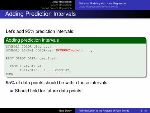
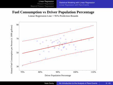
Adding Prediction Intervals
Let’s add 95% prediction intervals:
Adding prediction intervalsSYMBOL1 COLOR=blue ...;SYMBOL3 LINE=1 COLOR=red INTERPOL=rlcli ...;
PROC GPLOT DATA=home.fuel;...PLOT fuel*dlic=1;
fuel*dlic=3 / ... OVERLAY;RUN;
95% of data points should be within these intervals.
Should hold for future data points!
Nate Derby An Introduction to the Analysis of Rare Events 8 / 43
Linear RegressionPoisson Regression
Beyond Poisson Regression
Statistical Modeling with Linear RegressionLinear Regression with Rare Events
Ann
ual F
uel C
onsu
mpt
ion
per
Pers
on (
x 10
00 g
allo
ns)
30
50
70
90
Driver Population Percentage
70% 80% 90% 100% 110%
Fuel Consumption vs Driver Population PercentageLinear Regression Line + 95% Prediction Bounds
Nate Derby An Introduction to the Analysis of Rare Events 9 / 43
Linear RegressionPoisson Regression
Beyond Poisson Regression
Statistical Modeling with Linear RegressionLinear Regression with Rare Events
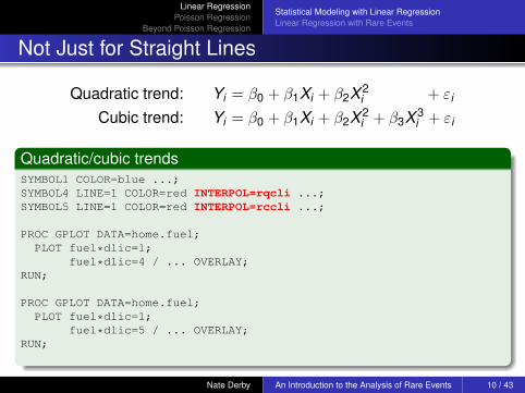
Not Just for Straight Lines
Quadratic trend: Yi = β0 + β1Xi + β2X 2i + εi
Cubic trend: Yi = β0 + β1Xi + β2X 2i + β3X 3
i + εi
Quadratic/cubic trendsSYMBOL1 COLOR=blue ...;SYMBOL4 LINE=1 COLOR=red INTERPOL=rqcli ...;SYMBOL5 LINE=1 COLOR=red INTERPOL=rccli ...;
PROC GPLOT DATA=home.fuel;PLOT fuel*dlic=1;
fuel*dlic=4 / ... OVERLAY;RUN;
PROC GPLOT DATA=home.fuel;PLOT fuel*dlic=1;
fuel*dlic=5 / ... OVERLAY;RUN;
Nate Derby An Introduction to the Analysis of Rare Events 10 / 43
Linear RegressionPoisson Regression
Beyond Poisson Regression
Statistical Modeling with Linear RegressionLinear Regression with Rare Events
Ann
ual F
uel C
onsu
mpt
ion
per
Pers
on (
x 10
00 g
allo
ns)
30
50
70
90
Driver Population Percentage
70% 80% 90% 100% 110%
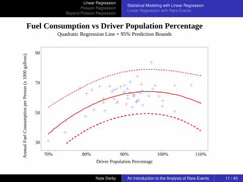
Fuel Consumption vs Driver Population PercentageQuadratic Regression Line + 95% Prediction Bounds
Nate Derby An Introduction to the Analysis of Rare Events 11 / 43
Linear RegressionPoisson Regression
Beyond Poisson Regression
Statistical Modeling with Linear RegressionLinear Regression with Rare Events
Ann
ual F
uel C
onsu
mpt
ion
per
Pers
on (
x 10
00 g
allo
ns)
30
50
70
90
Driver Population Percentage
70% 80% 90% 100% 110%
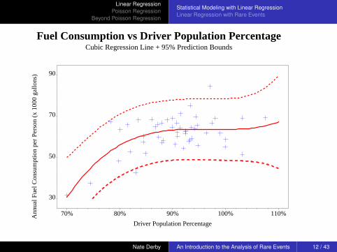
Fuel Consumption vs Driver Population PercentageCubic Regression Line + 95% Prediction Bounds
Nate Derby An Introduction to the Analysis of Rare Events 12 / 43
Linear RegressionPoisson Regression
Beyond Poisson Regression
Statistical Modeling with Linear RegressionLinear Regression with Rare Events
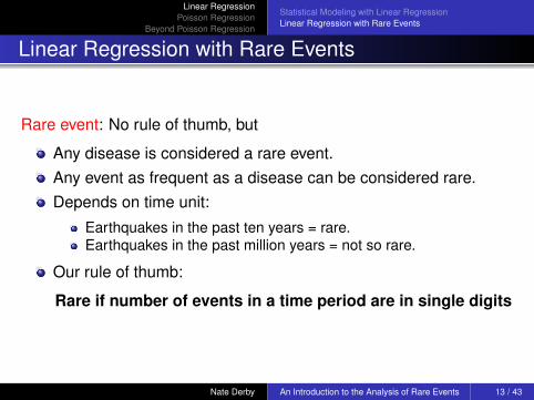
Linear Regression with Rare Events
Rare event: No rule of thumb, but
Any disease is considered a rare event.Any event as frequent as a disease can be considered rare.Depends on time unit:
Earthquakes in the past ten years = rare.Earthquakes in the past million years = not so rare.
Our rule of thumb:
Rare if number of events in a time period are in single digits
Nate Derby An Introduction to the Analysis of Rare Events 13 / 43
Linear RegressionPoisson Regression
Beyond Poisson Regression
Statistical Modeling with Linear RegressionLinear Regression with Rare Events
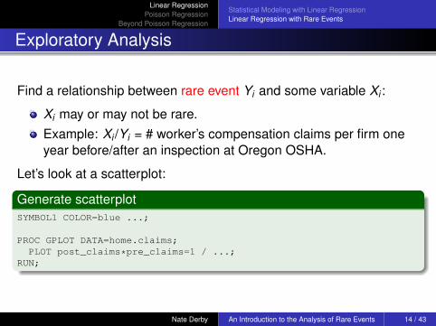
Exploratory Analysis
Find a relationship between rare event Yi and some variable Xi :
Xi may or may not be rare.Example: Xi /Yi = # worker’s compensation claims per firm oneyear before/after an inspection at Oregon OSHA.
Let’s look at a scatterplot:
Generate scatterplotSYMBOL1 COLOR=blue ...;
PROC GPLOT DATA=home.claims;PLOT post_claims*pre_claims=1 / ...;
RUN;
Nate Derby An Introduction to the Analysis of Rare Events 14 / 43
Linear RegressionPoisson Regression
Beyond Poisson Regression
Statistical Modeling with Linear RegressionLinear Regression with Rare Events
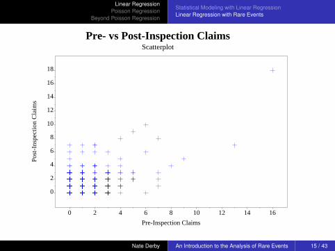
Post
-Ins
pect
ion
Cla
ims
0
2
4
6
8
10
12
14
16
18
Pre-Inspection Claims
0 2 4 6 8 10 12 14 16
Pre- vs Post-Inspection ClaimsScatterplot
Nate Derby An Introduction to the Analysis of Rare Events 15 / 43
Linear RegressionPoisson Regression
Beyond Poisson Regression
Statistical Modeling with Linear RegressionLinear Regression with Rare Events
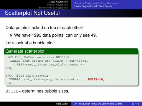
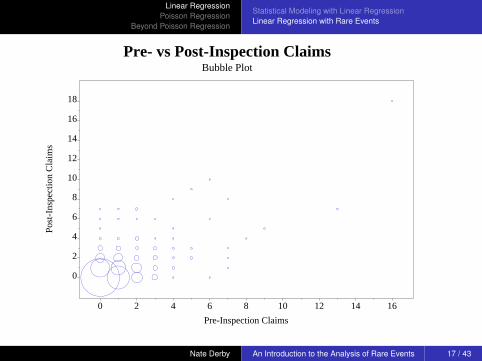
Scatterplot Not Useful
Data points stacked on top of each other!
We have 1293 data points, can only see 49.
Let’s look at a bubble plot:
Generate scatterplotPROC FREQ DATA=home.claims NOPRINT;TABLES post_claims*pre_claims / out=stats1
( KEEP=post_claims pre_claims count );RUN;
PROC GPLOT DATA=stats1;BUBBLE post_claims*pre_claims=count / ... BSIZE=10;
RUN;
BSIZE= determines bubble sizes.
Nate Derby An Introduction to the Analysis of Rare Events 16 / 43
Linear RegressionPoisson Regression
Beyond Poisson Regression
Statistical Modeling with Linear RegressionLinear Regression with Rare Events
Post
-Ins
pect
ion
Cla
ims
0
2
4
6
8
10
12
14
16
18
Pre-Inspection Claims
0 2 4 6 8 10 12 14 16
Pre- vs Post-Inspection ClaimsBubble Plot
Nate Derby An Introduction to the Analysis of Rare Events 17 / 43
Linear RegressionPoisson Regression
Beyond Poisson Regression
Statistical Modeling with Linear RegressionLinear Regression with Rare Events
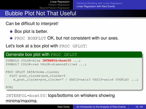
Bubble Plot Not That Useful
Can be difficult to interpret!
Box plot is better.PROC BOXPLOT OK, but not consistent with our axes.
Let’s look at a box plot with PROC GPLOT:
Generate box plot with PROC GPLOTSYMBOL6 COLOR=blue INTERPOL=boxt00 ...;SYMBOL7 COLOR=red VALUE=diamondfilled ...;
PROC GPLOT DATA=home.claims;PLOT post_claims*pre_claims=6m_post_claims*pre_claims=7 / HAXIS=axis3 VAXIS=axis4 OVERLAY ...;
RUN;
INTERPOL=boxt00: tops/bottoms on whiskers showingminima/maxima.
Nate Derby An Introduction to the Analysis of Rare Events 18 / 43
Linear RegressionPoisson Regression
Beyond Poisson Regression
Statistical Modeling with Linear RegressionLinear Regression with Rare Events
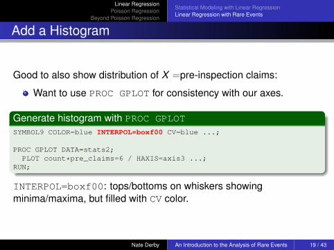
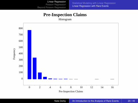
Add a Histogram
Good to also show distribution of X =pre-inspection claims:
Want to use PROC GPLOT for consistency with our axes.
Generate histogram with PROC GPLOTSYMBOL9 COLOR=blue INTERPOL=boxf00 CV=blue ...;
PROC GPLOT DATA=stats2;PLOT count*pre_claims=6 / HAXIS=axis3 ...;
RUN;
INTERPOL=boxf00: tops/bottoms on whiskers showingminima/maxima, but filled with CV color.
Nate Derby An Introduction to the Analysis of Rare Events 19 / 43
Linear RegressionPoisson Regression
Beyond Poisson Regression
Statistical Modeling with Linear RegressionLinear Regression with Rare Events
Freq
uenc
y
0
100
200
300
400
500
600
700
800
Pre-Inspection Claims
0 2 4 6 8 10 12 14 16
Pre-Inspection ClaimsHistogram
Nate Derby An Introduction to the Analysis of Rare Events 20 / 43
Linear RegressionPoisson Regression
Beyond Poisson Regression
Statistical Modeling with Linear RegressionLinear Regression with Rare Events
Post
-Ins
pect
ion
Cla
ims
0
2
4
6
8
10
12
14
16
18
Pre-Inspection Claims
0 2 4 6 8 10 12 14 16
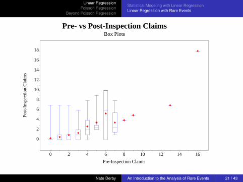
Pre- vs Post-Inspection ClaimsBox Plots
Nate Derby An Introduction to the Analysis of Rare Events 21 / 43

Linear RegressionPoisson Regression
Beyond Poisson Regression
Statistical Modeling with Linear RegressionLinear Regression with Rare Events
Observations
Data highly skewed (lopsided):
Right-skewed = right-tailed = mean > median.Pre-inspection claims X really right skewed.X = 3,4,5,7: Post-inspection claims Y really right skewed.X = 0: Y very right skewed: min to 75th percentile all at Y = 0.(no box)X = 1,2: Y very right skewed: min to median all at Y = 0.(half box)X =other: Too few data points to be important.
Data get less skewed for larger values of X .How good a fit does linear regression give us?
Nate Derby An Introduction to the Analysis of Rare Events 22 / 43
Linear RegressionPoisson Regression
Beyond Poisson Regression
Statistical Modeling with Linear RegressionLinear Regression with Rare Events
Post
-Ins
pect
ion
Cla
ims
0
2
4
6
8
10
12
14
16
18
Pre-Inspection Claims
0 2 4 6 8 10 12 14 16
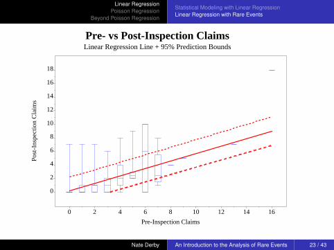
Pre- vs Post-Inspection ClaimsLinear Regression Line + 95% Prediction Bounds
Nate Derby An Introduction to the Analysis of Rare Events 23 / 43
Linear RegressionPoisson Regression
Beyond Poisson Regression
Statistical Modeling with Linear RegressionLinear Regression with Rare Events
Post
-Ins
pect
ion
Cla
ims
0
2
4
6
8
10
12
14
16
18
Pre-Inspection Claims
0 2 4 6 8 10 12 14 16
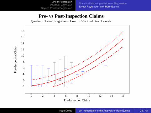
Pre- vs Post-Inspection ClaimsQuadratic Linear Regression Line + 95% Prediction Bounds
Nate Derby An Introduction to the Analysis of Rare Events 24 / 43

Linear RegressionPoisson Regression
Beyond Poisson Regression
Statistical Modeling with Linear RegressionLinear Regression with Rare Events
Post
-Ins
pect
ion
Cla
ims
0
2
4
6
8
10
12
14
16
18
Pre-Inspection Claims
0 2 4 6 8 10 12 14 16
Pre- vs Post-Inspection ClaimsCubic Linear Regression Line + 95% Prediction Bounds
Nate Derby An Introduction to the Analysis of Rare Events 25 / 43

Linear RegressionPoisson Regression
Beyond Poisson Regression
Statistical Modeling with Linear RegressionLinear Regression with Rare Events
How Well Does Our Model Fit?
The lines go through the boxes, right?
The median is usually below the regression line, so more than50% of the data is below that line.Prediction bounds are symmetric around the regression line.
Data are not symmetric around the median values. This is afundamental mismatch
Data outside the 95% prediction bounds. Is that around 5%?
We have a wrong trend line and a false level of accuracy.
Linear regression doesn’t work, and we’d like a smooth trend line.
Nate Derby An Introduction to the Analysis of Rare Events 26 / 43

Linear RegressionPoisson Regression
Beyond Poisson Regression
Statistical Modeling with Linear RegressionLinear Regression with Rare Events
Post
-Ins
pect
ion
Cla
ims
0
2
4
6
8
10
12
14
16
18
Pre-Inspection Claims
0 2 4 6 8 10 12 14 16
Pre- vs Post-Inspection ClaimsConnecting the Means
Nate Derby An Introduction to the Analysis of Rare Events 27 / 43
Linear RegressionPoisson Regression
Beyond Poisson Regression
Fitting the ModelInterpreting the ResultsGetting Predicted Counts
Poisson Regression
Solution is easy:
Use a similar process to linear regression, but ...Instead of symmetric continuous distribution, use a skewed,discrete one!We’re just applying a theoretical distribution that better fits thedata.
Nate Derby An Introduction to the Analysis of Rare Events 28 / 43
Linear RegressionPoisson Regression
Beyond Poisson Regression
Fitting the ModelInterpreting the ResultsGetting Predicted Counts
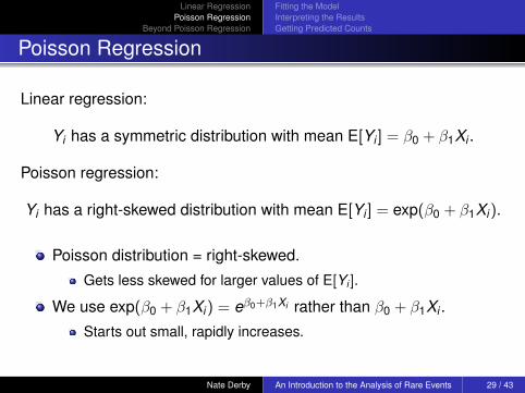
Poisson Regression
Linear regression:
Yi has a symmetric distribution with mean E[Yi ] = β0 + β1Xi .
Poisson regression:
Yi has a right-skewed distribution with mean E[Yi ] = exp(β0 + β1Xi).
Poisson distribution = right-skewed.
Gets less skewed for larger values of E[Yi ].
We use exp(β0 + β1Xi) = eβ0+β1Xi rather than β0 + β1Xi .
Starts out small, rapidly increases.
Nate Derby An Introduction to the Analysis of Rare Events 29 / 43
Linear RegressionPoisson Regression
Beyond Poisson Regression
Fitting the ModelInterpreting the ResultsGetting Predicted Counts
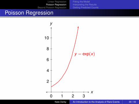
Poisson Regression
y = exp(x)
x
y
0 1 2 3
2
4
6
8
10
Nate Derby An Introduction to the Analysis of Rare Events 30 / 43
Linear RegressionPoisson Regression
Beyond Poisson Regression
Fitting the ModelInterpreting the ResultsGetting Predicted Counts
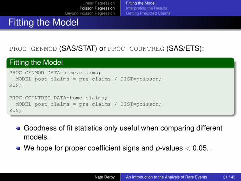
Fitting the Model
PROC GENMOD (SAS/STAT) or PROC COUNTREG (SAS/ETS):
Fitting the ModelPROC GENMOD DATA=home.claims;MODEL post_claims = pre_claims / DIST=poisson;
RUN;
PROC COUNTREG DATA=home.claims;MODEL post_claims = pre_claims / DIST=poisson;
RUN;
Goodness of fit statistics only useful when comparing differentmodels.We hope for proper coefficient signs and p-values < 0.05.
Nate Derby An Introduction to the Analysis of Rare Events 31 / 43

Linear RegressionPoisson Regression
Beyond Poisson Regression
Fitting the ModelInterpreting the ResultsGetting Predicted Counts
PROC GENMOD Output
The GENMOD Procedure
Model Information
Data Set HOME.CLAIMSDistribution PoissonLink Function LogDependent Variable post_claims Post-Inspection
Claims
Number of Observations Read 1310Number of Observations Used 1293Missing Values 17
Nate Derby An Introduction to the Analysis of Rare Events 32 / 43

Linear RegressionPoisson Regression
Beyond Poisson Regression
Fitting the ModelInterpreting the ResultsGetting Predicted Counts
PROC GENMOD Output
Criteria For Assessing Goodness Of Fit
Criterion DF Value Value/DF
Deviance 1291 1623.3440 1.2574Scaled Deviance 1291 1623.3440 1.2574Pearson Chi-Square 1291 2070.2270 1.6036Scaled Pearson X2 1291 2070.2270 1.6036Log Likelihood -972.7283Full Log Likelihood -1309.5635AIC (smaller is better) 2623.1270AICC (smaller is better) 2623.1363BIC (smaller is better) 2623.4564
Algorithm converged.
Nate Derby An Introduction to the Analysis of Rare Events 33 / 43
Linear RegressionPoisson Regression
Beyond Poisson Regression
Fitting the ModelInterpreting the ResultsGetting Predicted Counts
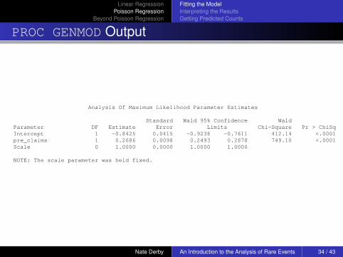
PROC GENMOD Output
Analysis Of Maximum Likelihood Parameter Estimates
Standard Wald 95% Confidence WaldParameter DF Estimate Error Limits Chi-Square Pr > ChiSqIntercept 1 -0.8425 0.0415 -0.9238 -0.7611 412.14 <.0001pre_claims 1 0.2686 0.0098 0.2493 0.2878 749.10 <.0001Scale 0 1.0000 0.0000 1.0000 1.0000
NOTE: The scale parameter was held fixed.
Nate Derby An Introduction to the Analysis of Rare Events 34 / 43
Linear RegressionPoisson Regression
Beyond Poisson Regression
Fitting the ModelInterpreting the ResultsGetting Predicted Counts
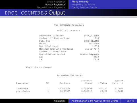
PROC COUNTREG Output
The COUNTREG Procedure
Model Fit Summary
Dependent Variable post_claimsNumber of Observations 1293Data Set HOME.CLAIMSModel PoissonLog Likelihood -1310Maximum Absolute Gradient 2.24243E-7Number of Iterations 5Optimization Method Newton-RaphsonAIC 2623SBC 2633
Algorithm converged.
Parameter Estimates
Standard ApproxParameter DF Estimate Error t Value Pr > |t|
Intercept 1 -0.842474 0.041499 -20.30 <.0001pre_claims 1 0.268575 0.009813 27.37 <.0001
Nate Derby An Introduction to the Analysis of Rare Events 35 / 43
Linear RegressionPoisson Regression
Beyond Poisson Regression
Fitting the ModelInterpreting the ResultsGetting Predicted Counts
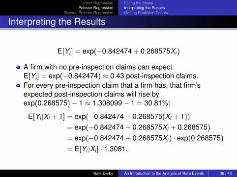
Interpreting the Results
E[Yi ] = exp(−0.842474 + 0.268575Xi)
A firm with no pre-inspection claims can expectE[Yi ] = exp(−0.842474) ≈ 0.43 post-inspection claims.For every pre-inspection claim that a firm has, that firm’sexpected post-inspection claims will rise byexp(0.268575)− 1 ≈ 1.308099− 1 = 30.81%:
E[Yi |Xi + 1] = exp(−0.842474 + 0.268575(Xi + 1))= exp(−0.842474 + 0.268575Xi + 0.268575)= exp(−0.842474 + 0.268575Xi) · exp(0.268575)= E[Yi |Xi ] · 1.3081.
Nate Derby An Introduction to the Analysis of Rare Events 36 / 43
Linear RegressionPoisson Regression
Beyond Poisson Regression
Fitting the ModelInterpreting the ResultsGetting Predicted Counts
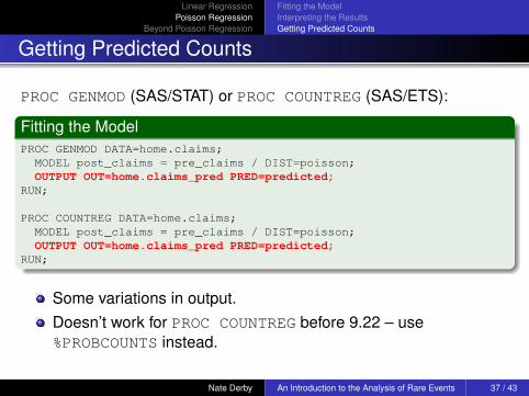
Getting Predicted Counts
PROC GENMOD (SAS/STAT) or PROC COUNTREG (SAS/ETS):
Fitting the ModelPROC GENMOD DATA=home.claims;MODEL post_claims = pre_claims / DIST=poisson;OUTPUT OUT=home.claims_pred PRED=predicted;
RUN;
PROC COUNTREG DATA=home.claims;MODEL post_claims = pre_claims / DIST=poisson;OUTPUT OUT=home.claims_pred PRED=predicted;
RUN;
Some variations in output.Doesn’t work for PROC COUNTREG before 9.22 – use%PROBCOUNTS instead.
Nate Derby An Introduction to the Analysis of Rare Events 37 / 43

Linear RegressionPoisson Regression
Beyond Poisson Regression
Fitting the ModelInterpreting the ResultsGetting Predicted Counts
Post
-Ins
pect
ion
Cla
ims
0
2
4
6
8
10
12
14
16
18
Pre-Inspection Claims
0 2 4 6 8 10 12 14 16
Pre- vs Post-Inspection ClaimsPoisson Regression Line
Nate Derby An Introduction to the Analysis of Rare Events 38 / 43
Linear RegressionPoisson Regression
Beyond Poisson Regression
Fitting the ModelInterpreting the ResultsGetting Predicted Counts
Post
-Ins
pect
ion
Cla
ims
0
2
4
6
8
10
12
14
16
18
Pre-Inspection Claims
0 2 4 6 8 10 12 14 16
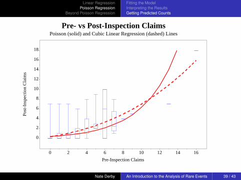
Pre- vs Post-Inspection ClaimsPoisson (solid) and Cubic Linear Regression (dashed) Lines
Nate Derby An Introduction to the Analysis of Rare Events 39 / 43
Linear RegressionPoisson Regression
Beyond Poisson Regression
Fitting the ModelInterpreting the ResultsGetting Predicted Counts
How Did We Do?
This is a smooth line!Poisson regression line very close to most of the median values.(Better than hitting the mean values, since the median is robustagainst outliers and we have skewed distributions)The Poisson regression fit even comes close to the singularvalues at X = 8 and X = 9.
Poisson regression fit is a better fit that any of the three linearregression models!
Nate Derby An Introduction to the Analysis of Rare Events 40 / 43
Linear RegressionPoisson Regression
Beyond Poisson Regression
Beyond Poisson Regression
Poisson regression has a couple serious limitations:
Assumes mean = variance, often not the case.Often more zeroes than the model can handle.
These problems are addressed by negative binomial regression andzero-inflated Poisson/negative binomial regression.
Nate Derby An Introduction to the Analysis of Rare Events 41 / 43

Linear RegressionPoisson Regression
Beyond Poisson Regression
Beyond Poisson Regression
BTW ...
This analysis does not isolate the effect of inspections.This analysis does not show that inspections have an effect.We need a control group→ propensity score matching.
Nate Derby An Introduction to the Analysis of Rare Events 42 / 43
Appendix
Further Resources
Sanford Weisberg.Applied Linear Regression.Wiley, 2005.
Russ Lavery.An Animated Guide: An Introduction to Poisson Regression.Proceedings of the Twenty-Third NESUG Conference, 2010.
Nate Derby: [email protected]
Nate Derby An Introduction to the Analysis of Rare Events 43 / 43