Embed Size (px)
Citation preview

ANALYTICAL AND SIMULATION PERFORMANCE MODELLING OF INDOOR INFRARED WIRELESS DATA
COMMUNICATIONS PROTOCOLS
PETER JAY BARKER
A thesis submitted in partial fulfilment of the requirements of Bournemouth University for the degree of Doctor of Philosophy
April 2003
I
Bournemouth University
BOURNEMOUTH! V-"--, "~R, SI"I'Y
LirýývARY D36/y. 64-6
aza Lro2-N.
382 ý8A'ý
IA 00 1k 6t tXýp
11

Abstract
The Infrared (IR) optical medium provides an alternative to radio frequencies (RF) for low cost, low power and short-range indoor wireless data communications. Low-cost optoelectronic components with an unregulated IR spectrum provide the potential for very high-speed wireless communication with good security. However IR links have a limited range and are susceptible to high noise levels from ambient light sources. The Infrared Data Association (IrDA) has produced a set of communication protocol standards (IrDA I. x) for directed point-to-point IR wireless links using a HDLC (High- level Data Link Control) based data link layer which have been widely adopted. To address the requirement for multi-point ad-hoc wireless connectivity, IrDA have produced a new standard (Advanced Infrared - AIr) to support multiple-device non- directed IR Wireless Local Area Networks (WLANs). AIr employs an enhanced physical layer and a CSMA/CA (Carrier Sense Multiple Access with Collision Avoidance) based MAC (Media Access Control) layer employing RTS/CTS (Request To Send / Clear To Send) media reservation.
This thesis is concerned with the design of IrDA based IR wireless links at the data link layer, media access sub-layer, and physical layer and presents protocol performance models with the aim of highlighting the critical factors affecting performance and providing recommendations to system designers for parameter settings and protocol enhancements to optimise performance.
An analytical model of the IrDA 1. x data link layer (IrLAP - Infrared Link Access Protocol) using Markov analysis of the transmission window width providing saturation condition throughput in relation to the link bit-error-rate (BER), data rate and protocol parameter settings is presented. Results are presented for simultaneous optimisation of the data packet size and transmission window size. A simulation model of the IrDA l. x protocol, developed with OPNETTM Modeler, is used for validation of analytical results and to produce non-saturation throughput and delay performance results.
An analytical model of the AIr MAC protocol providing saturation condition utilisation and delay results in relation to the number of contending devices and MAC protocol parameters is presented. Results indicate contention window size values for optimum utilisation. The effectiveness of the AIr contention window linear back-off process is examined through Markov analysis. An OPNET simulation model of the Alf protocol is used for validation of the analytical model results and provides non-reservation throughput and delay results.
An analytical model of the IR link physical layer is presented and derives expressions for signal-to-noise ratio (SNR) and BER in relation to link transmitter and receiver characteristics, link geometry, noise levels and line encoding schemes. The effect of third user interference on BER and resulting link asymmetry is also examined, indicating the minimum separation distance for adjacent links. Expressions for BER are linked to the data link layer analysis to provide optimum throughput results in relation to physical layer properties and link distance.
iii

Table of contents
Acknowledgements ..................................................................................................... viii
Accompanying Material ............................................................................................... ix
Abbreviations ............................................................................................................... xii
List of Figures ............................................................................................................. xiv
List of Tables ............................................................................................................. xvii
1. INTRODUCTION ........................................................................................................ 1
1.1 Background and Motivation .................................................................................... 1
1.2 Statement of Problem .............................................................................................. 5
1.3 Outline of Research ................................................................................................. 6
1.4 Thesis Format .......................................................................................................... 8
2. BACKGROUND INFORMATION ........................................................................... 11
2.1 Wireless Communications Media .......................................................................... 11
2.1.2 History of IR Wireless Systems ...................................................................... 12
2.1.3 IR Wireless Links ............................................................................................ 2.1.3.1 Binary Modulation and Encoding ................................................................ 14
2.1.3.2 Noise and Error Detection ........................................................................... 15
2.1.4 Classification of IR Wireless Links ................................................................. 16
2.1.5 IR Wireless Communication Networks ........................................................... 17
2.2 Communications Protocols .................................................................................... 18
2.2.1 Protocol Stack Reference Model ..................................................................... 18 2.2.2 Data Link Protocols ......................................................................................... 19 2.2.3 Media Access Protocols .................................................................................. 20
2.3 Current IR Wireless Protocols ............................................................................... 22 2.3.1 The IrDA 1. x Protocol ..................................................................................... 22 2.3.2 The Advanced Infrared (AIr) Protocol ............................................................ 23 2.3.3 The IEEE 802.11 IR-WLAN Standard ............................................................ 24
2.4 Performance Modelling of Communications Systems .......................................... 24 2.5 Chapter Summary ..................................................................................................
27
3. IR WIRELESS COMMUNICATIONS PROTOCOLS .............................................. 29
3.1 The IrDA l. x Protocol ........................................................................................... 29 3.1.1 The IrDA 1. x Physical Layer ......................................................................... 30 3.1.1.1 IrDA SIR Physical Layer 2400 to 115,200 bits/s ......................................... 30 3.1.1.2 IrDA FIR Physical Layer 0.576,1.152 and 4 Mbits/s .................................. 31 3.1.1.3 IrDA VFIR Physical Layer 16 Mbits/s ........................................................ 32 3.1.2 The IrLAP Layer .............................................................................................
33 3.1.2.1 IrLAP Frame Format .................................................................................... 34 3.1.2.2 IrLAP Connection Establishment
................................................................. 37
3.1.2.3 IrLAP Information Exchange Procedure ...................................................... 38 3.1.2.4 IrLAP Extension for 16 Mbits/s VFIR .........................................................
42 3.1.3 Other IrLAP Components ...............................................................................
43 3.2 The Advanced Infrared (AIr) Protocol ..................................................................
44
iv

3.2.1 The AIr Physical Layer ................................................................................... 44 3.2.2 The AIr MAC Protocol ....................................................................................
46 3.2.2.1 The AIr MAC Frame Structure ....................................................................
46 3.2.2.2 AIr MAC Finite State Machine ....................................................................
48 3.2.2.3 AIr MAC Reserved Mode Data Transfer .....................................................
49 3.2.2.4 AIr MAC Unreserved, Announced and Proxy Modes .................................
53 3.2.3 The AIr LM Layer ...........................................................................................
55 3.2.4 The AIr LC Layer ............................................................................................
56 3.3 Chapter Summary
.................................................................................................. 56
4. PHYSICAL LAYER ANALYSIS .............................................................................. 57
4.1 IR Channel Model ..................................................................................................
57 4.1.1 Transmitted Optical Power
.............................................................................. 59
4.1.2 Received Optical Power .................................................................................. 61
4.1.3 Signal-to-Noise Ratio ......................................................................................
62 4.2 Modelling Noise Sources
....................................................................................... 62
4.2.1 Ambient Light Induced Shot Noise ................................................................. 63
4.2.2 Thermal Noise ............... ..............................................................................
65 4.3 BER and Packet Errors ..........................................................................................
67 4.3.1 Required Bandwidth ........................................................................................
68 4.3.2 IrDA SIR RZI Modulation ..............................................................................
69 4.3.3 FIR 4Mbits/s 4PPM Modulation
..................................................................... 70
4.3.4 VFIR 16 Mbits/s Rate 2/3 (1,13 15) RLL HHH Encoding ............................ 71
4.3.5 Example Implementation and Performance Calculation ................................. 74
4.3.6 Approximation of BER ................................................................................... 76
4.3.7 4PPM -Variable Symbol Repetition ...............................................................
77 4.4 Third User Interference ..........................................................................................
79 4.4.1 Directional Asymmetry from Third User Interference ....................................
82 4.4.2 Spatial Asymmetry from Moveable Link with Fixed Interferer .....................
84 4.5 Chapter Summary
.................................................................................................. 88
5. MODELLING OF COMMUNICATIONS PROTOCOLS ........................................ 89
5.1 Modelling HDLC Based Data Link Protocols ....................................................... 89
5.1.1 The Virtual Transmission Time Method ......................................................... 89
5.1.2 Queuing Analysis Method ............................................................................... 92
5.1.3 Probabilistic Automaton ..................................................................................
93 5.1.4 Simulation Studies of HDLC ..........................................................................
95 5.2 Modelling CSMA/CA Medium Access Protocols .................................................
96 5.2.1 Performance Models of CSMA/CA
................................................................ 96
5.3 Chapter Summary ................................................................................................ 100
6. IRDA LX PROTOCOL PERFORMANCE MODELLING ..................................... 101
6.1 IrDA IrLAP Analytical Model ....................... ............... 101 ....................................... 6.1.1 Model Assumptions and Parameters .............................................................
102 6.1.2 Calculation of the Virtual Transmission Time ..............................................
104 6.1.2.1 Window Width Probability ........................................................................
104

6.1.2.2 Window Width Dependent Virtual Transmission Time ............................ 107 6.1.2.3 Bi-directional Data Flow Throughput ........................................................ 113 6.1.2.4 F-timer Duration ......................................................................................... 113 6.1.3 Optimum Packet Length and Window Size .................................................. 114 6.1.4 Validation of IrLAP Analytical model .......................................................... 117
6.2 IrLAP Analysis Results ....................................................................................... 118 6.2.1 IrDA SIR 115.2 kbits/s Analysis ................................................................... 118 6.2.2 IrDA FIR 4 Mbits/s Analysis ........................................................................ 124 6.2.3 IrDA VFIR 16 Mbits/s Analysis ...................................................................
129 6.3 IrDA 1. x Simulation Model Results .................................................................... 135
6.3.1 IrDA I .x Delay Results ................................................................................. 135 6.3.2 IrDA l. x Non-saturation Results ................................................................... 137
6.4 Chapter Summary ................................................................................................ 138
7. AIR MAC PROTOCOL PERFORMANCE MODELLING .................................... 139
7.1 AIr MAC Analytical Model ................................................................................. 139
7.1.1 Model Parameters and Assumptions ............................................................. 139
7.1.2 Utilisation Calculation ................................................................................... 141
7.1.3 Average Burst Delay ..................................................................................... 143
7.1.4 Markov Model of Collision Avoidance Back-off Mechanism ...................... 144
7.2 AIr MAC Performance Results ........................................................................... 151
7.2.1 AIr MAC Reserved Mode Analysis .............................................................. 151
7.2.2 Validation of AIr MAC Analysis results ....................................................... 156 7.2.3 AIr MAC Unreserved Simulation Results .................................................... 157
7.3 Chapter Summary ................................................................................................ 159
8. CONCLUSIONS AND FURTHER WORK ............................................................. 161
8.1 Summary of Thesis .............................................................................................. 161 8.2 IrDA 1. x Analysis Conclusions ........................................................................... 162 8.3 IR Physical Layer Conclusions ............................................................................ 164 8.4 AIr Analysis Conclusions .................................................................................... 165 8.5 Suggestions for Further Research ........................................................................ 166
8.5.1 Further IrDA Protocol Research .................................................................... 166 8.5.2 Further AIr Protocol Research ...................................................................... 168
APPENDIX A OPNET SIMULATION MODELS ...................................................... 169
A. 1 The OPNET Modeler package ............................................................................ 169 A. 2 The IrDA Lx OPNET Simulation Model ........................................................... 172
A. 2.1 IrDA Model Network Level ......................................................................... 172 A. 2.2 IrDA Model Packet Format .......................................................................... 173 A. 2.3 IrLAP Basic Model ....................................................................................... 173 A. 2.3.1 IrDA Basic Model Node Level ..................................................................
174 A. 2.3.2 IrLAP Basic model process level .............................................................. 174 A. 2.3.3 IrDA Basic Model simulation Execution .................................................. 177 A. 2.4 IrLAP Advanced Model ............................................................................... 178 A. 2.4.1 IrLAP Advanced Model Node Level ........................................................
179
vi

A. 2.4.2 IrDA Source and Sink Models .................................................................. 179
A. 2.4.3 IrLAP Primary Station Advanced Process Model ..................................... 179
A. 2.4.4 Advanced Model Simulation Execution .................................................... 181
A. 3 AIr OPNET Model .............................................................................................. 182
A. 3.1 AIr Model Network Level ............................................................................ 182
A. 3.2 AIr Station Node Model ............................................................................... 184
A. 3.3. AIr LM Process Model ................................................................................ 184
A. 3.4 AIr MAC Process Model .............................................................................. 186
A. 3.5 The AIr Physical Layer Interface Process Model ......................................... 187
A. 3.6 The AIr Monitor Node and Process Models ................................................. 187
A. 3.7 AIr Model Attributes and Statistics .............................................................. 188
APPENDIX B LIMITING DISTRIBUTION OF A MARKOV CHAIN ..................... 189
APPENDIX C GAUSSIAN TAIL INTEGRAL, Q- FUNCTION .............................. 191
REFERENCES .............................................................................................................. 193
vii

Acknowledgements
Special thanks to my supervisor Professor Tony Boucouvalas
Thank to Colin Millar, Steve Buttery and Ian Nield at BT labs, Martlesham for initial financial and supervisory support for this project.
To my friends, colleagues, office co-habitants and fellow researchers (in no particular
order): Glyn Hadley, Simon Crowle, Jenny Longster, Daniel Vine, Paul and Ruth
Nicholson, Carolyn Mair, Tom Teng, David John, Colin Murphy, Periklis Chatzimisios,
Vasileios Vitsas, Martin Teal, Tim Orman, Paul Rogers.
To Mum and Ced, Dad and Angelika, Sally and Mark
viii

Accompanying Material
The following papers were published during the course of the research conducted for
this thesis.
Journal Publications
[1] Vitsas, V., Barker, P. & Boucouvalas, A. C. (2003), "IrDA Infrared Wireless
Communications: Protocol Throughput Optimization", IEEE Wireless Communications,
Vol. 10, No 2, April 2003, pp. 22 - 29
[2] Barker, P. Vitsas, V. & Boucouvalas, A. C. (2002), "Simulation Analysis of the
Advanced Infrared (AIr) MAC Wireless Communications Protocol", IEE proceedings
Circuits- and Systems, Vol. 149, No 3, June 2002, pp. 193 -197.
[3] Barker, P. & Boucouvalas, A. C. (2000), "Asymmetry in Optical Wireless Links",
IEE Proceedings Optoelectronics, Vol. 147, No 4 August 2000, pp. 315 - 321.
[4] Barker, P. & Boucouvalas, A. C., (2000) "Performance Modelling of the IrDA
Infrared Wireless Communications Protocol", International Journal of Communications
Systems, Vol. 13, No 7-8, Nov-Dec 2000, pp. 589 - 604.
[5] Barker, P. & Boucouvalas, A. C. (1998), "IrLAP protocol performance analysis of
IrDA wireless communications", IEE Electronics letters, Vol. 34, No. 25, pp. 2380-
2381.
[6] Barker, P. & Boucouvalas, A. C. (1998), "Performance modelling of the IrDA
protocol for Infrared Wireless Communications", IEEE Communications magazine, Vol. 36, No. 12, December 1998, pp. 113-117.
IX

Conference Publications
[1] Barker, P. & Boucouvalas, A. C. (2002), "Interference Induced Asymmetry in IrDA
4PPM Infrared Wireless Links", 3rd International Symposium on Communication
Systems, Networks and Digital Signal Processing (CSNDSP 2002), University of
Staffordshire, Stafford, 15th - 17th July 2002, pp. 479 - 482.
[2] Barker, P. & Boucouvalas, A. C. (2002), "Directional and Spatial Asymmetry in
IrDA 4PPM Infrared Wireless Links with Third User Interference" 3rd Annual
postgraduate Symposium on the Convergence of Telecommunications, Networking and
Broadcasting (PGNET 2002), Liverpool John Moores University, 17th -18th June 2002,
pp. 353 - 358.
[3] Barker, P. & Boucouvalas, A. C. (2001), "Performance Comparison of the IEEE
802.11 and AIr Infrared Wireless MAC Protocols", 2nd Annual postgraduate
Symposium on the Convergence of Telecommunications, Networking and Broadcasting
(PGNET 2001), Liverpool John Moores University, 18th-19th June 2001, pp. 113 - 118.
[4] Barker, P. & Boucouvalas, A. C. (2000), "A Simulation Model of the Advanced
Infrared (AIr) MAC protocol using OPNET", 2nd International Symposium on Communication Systems, Networks and Digital Signal Processing (CSNDSP 2000),
Bournemouth University, 18th - 20th July 2000, pp. 153 -156.
[5] Barker, P. & Boucouvalas, A. C. (2000), "Modelling of the IrDA and AIr Wireless
Infrared Communications Protocols", Ist Annual postgraduate Symposium on the
Convergence of Telecommunications, Networking and Broadcasting (PGNET 2000),
Liverpool John Moores University, 19th - 20th June 2000, pp. 137 - 142.
[6] Barker, P. & Boucouvalas, A. C. (1999), "Asymmetric Throughput in Optical
Wireless Links", Second Electronic Circuits and Systems Conference, Bratislava,
Slovakia, September 1999, pp. 129-134.
X

[7] Barker, P. & Boucouvalas, A. C. (1999), "Asymmetric Throughput in IrDA Links",
IEE Colloquium on Optical Wireless Communications, Savoy Place, London, 22nd June
1999, pp. 7/1-5.
[8] Barker, P. & Boucouvalas, A. C., (1999), "Effect of Random Alignment Sway on
The Performance of IrDA Handheld Device Links", IEE Colloquium on Optical
Wireless Communications, Savoy Place, London, 22nd June, 1999, pp. 9/1-4.
[9] Barker, P. & Boucouvalas, A. C. (1998), "A Simulation Model of IrDA Infrared
Communication Protocol", Ist International Symposium on Communication Systems
and Digital Signal Processing, Sheffield Hallam University, 6-8 April 1998, pp. 2-5.
[10] Barker, P. & Boucouvalas, A. C. (1998), "Performance Analysis of the IrDA
Protocol in Wireless Communications", Ist International Symposium on
Communication Systems and Digital Signal Processing, Sheffield Hallam University, 6-
8 April 1998, pp. 6-9
[I I] Barker, P. & Boucouvalas, A. C. (1997), "IrDA Protocol Performance Analysis for
Short Range IR Data Communication", Fourth Communication Network Symposium,
Manchester Metropolitan University, 7 -8 July 1997, pp. 224 - 227.
X1

Abbreviations
ABM ACK AIr ARM ARQ BER BOF CAS CDMA CRC CSMA/CA CSMA/CD CTS Cw DCF DIFS EOB EOBC EOF FCS FIR FOV FSM FTC FTX HDLC IAS IEEE IM/DD IR IrDA IrLAP IrLMP ISI ISR LAN LC LED LM LSAP MAC MBR MUX NRM NRZ OOK
Asynchronous Balanced Mode Acknowledgement Advanced Infrared Asynchronous Response Mode Automatic Repeat-request Bit Error Rate Beginning-Of-Frame Collision Avoidance Slot Code Division Multiple Access Cyclic Redundancy Check Carrier Sense Multiple Access / Collision Avoidance Carrier Sense Multiple Access / Collision Detection Clear-To-Send Contention Window Distributed Co-ordination Function Distributed Interframe Space End-Of-Burst End-Of-Burst Confirm End-Of-Frame Frame Check Sequence Fast Infrared Field-of-View Finite State Machine Frame Transmission Complete Frame Transmit High-level Data Link Control Information Access Service Institute of Electrical and Electronic Engineers Intensity Modulation / Direct Detection Infrared Infrared Data Association Infrared Link Access Protocol Infrared Link Management Protocol Intersymbol Interference Interference-to-Signal Ratio Local Area Network Link Controller Light Emitting Diode Link Manager Link Service Access Point Medium Access Control Main Body Received Multiplexer Normal Response Mode Non Return-to-Zero On-Off Keying
X11

PCF Point Co-ordination Function PDA Personal Data Assistant PHY Physical Layer PIN Positive-Intrinsic-Negative PPM Pulse Position Modulation RF Radio Frequencies RHR Robust Header Received RR Repetition Rate or Receive Ready RTS Request-To-Send RZ Return-to-Zero RZI Return-to-Zero Inverted SIR Serial Infrared SNR Signal-to-Noise Ratio SOD Start-Of-Data SPOLL Sequenced-Polling VFIR Very Fast Infrared VR Variable Repetition VTT Virtual Transmission Time WLAN Wireless Local Area Network WPAN Wireless Personal Area Network
X111

List of Figures
Figure 2.1 Basic wireless infrared link ........................................................................... 13 Figure 2.2 Silicon relative spectral sensitivity versus wavelength ................................. 14 Figure 2.3 Classification of IR links ............................................................................... 16 Figure 2.4 Infrared wireless communication networks .................................................. 18 Figure 2.5 Standard HDLC frame structure .................................................................... 20 Figure 2.6 Throughput versus load for various media access schemes .......................... 22 Figure 3.1 The IrDA 1. x protocol stack .......................................................................... 29 Figure 3.2 IrDA PHY optical interface specification ..................................................... 30 Figure 3.3 IrDA PHY 1.0 schematic ............................................................................... 31 Figure 3.4 IrDA SIR PHY 9600 to 115,200 bits/s 3/16 RZI data format scheme.......... 31 Figure 3.5 IrDA PHY 1.1 schematic ............................................................................... 32 Figure 3.6 IrDA FIR PHY 4 Mbits/s 4PPM modulation scheme ................................... 32 Figure 3.7 IrLAP procedure flow .................................................................................... 34 Figure 3.8 IrLAP packet format ...................................................................................... 34 Figure 3.9 IrLAP U-frame control field .......................................................................... 35 Figure 3.10 IrLAP S-frame control field ........................................................................ 36 Figure 3.11 IrLAP I-frame control field .........................................................................
36 Figure 3.12 Primary station XMIT state frame transmission procedure ......................... 38 Figure 3.13 Primary station RECV state frame reception procedure ............................. 39 Figure 3.14 Primary station frame re-transmission process ............................................ 40 Figure 3.15 Example IrLAP transfers ............................................................................. 42 Figure 3.16 The AIr Protocol stack ................................................................................. 44 Figure 3.17 AIr optical interface specifications .............................................................. 45 Figure 3.18 Example variable repetition 4PPM encoding .............................................. 46 Figure 3.19 AIr MAC frame structure ............................................................................ 47 Figure 3.20 AIr MAC finite state diagram ..................................................................... 48 Figure 3.21 AIr MAC reserved mode data transfer process ........................................... 51 Figure 3.22 The hidden node problem ............................................................................ 52 Figure 3.23 AIr MAC reserved mode transfer methods ................................................. 53 Figure 3.24 AIr MAC data transfer modes ..................................................................... 54 Figure 3.25 AIr LM CAS back-off process .................................................................... 55 Figure 4.1 IM/DD transmission and reception model ..................................................... 57 Figure 4.2 IR Wireless channel model ............................................................................ 58 Figure 4.3 Solid angle geometry ..................................................................................... 59 Figure 4.4 Radiant intensity pattern for increasing n ..................................................... 60 Figure 4.5 Optical link geometry .................................................................................... 61 Figure 4.6 Normalised power spectra for ambient light sources .................................... 64 Figure 4.7 Basic transimpedance receiver preamplifier design ...................................... 65 Figure 4.8 IrDA SIR 3/16 RZI transmission and detection ............................................ 69 Figure 4.8 BER versus SNR for IrDA modulation schemes ........................................... 73 Figure 4.9 Packet capture probability versus SNR for IrDA modulation schemes ........ 73 Figure 4.10 Bit error rate versus link LOS distance for IrDA links
................................ 75 Figure 4.11 Packet capture probability versus LOS distance for IrDA links ................. 75 Figure 4.12 BER versus LOS distance with IrDA BER approximation ......................... 76 Figure 4.13 Packet capture probability versus SNR for 4PPM/VR ................................ 78
XIV
Figure 4.14 Packet error probability versus link LOS distance for 4 Mbits/s 4PPM/VR modulation ................................................................................................................ 79
Figure 4.15 Raised cosine interference pulse with quantisation ISR levels ................... 80
Figure 4.16 4PPM packer error probability versus SNR for varying ISR levels............ 82 Figure 4.17 Directional asymmetry model geometry ......................................................
83 Figure 4.18 Directional BER asymmetry versus interferer approach distance ...............
84 Figure 4.19 Interferer loci for constant BER values with narrow angle transceivers .....
84 Figure 4.20 Geometry of spatial asymmetry scenario ....................................................
85 Figure 4.21 Spatial asymmetry for user C loci and AB separation distance d to provide
BER < 10"8 ................................................................................................................ 87
Figure 5.1 HDLC window width process fmite state diagram ........................................ 91
Figure 5.2 HDLC half-duplex NRM finite state process and goal process .................... 94
Figure 5.3 Basic and RTS/CTS access times for 802.11 DCF ....................................... 99
Figure 6.1 Window width states for N=7.................................................................... 105 Figure 6.2 Markov process diagram for IrLAP window width process ........................
105 Figure 6.3 Case A transmission times ..........................................................................
108 Figure 6.4 Case B(i) re-transmission time ...................................................................
109 Figure 6.5 Case B(ii) re-transmission time ...................................................................
110 Figure 6.6 Simulation and analysis model results comparison for 4 Mbits/s IrDA link
................................................................................................................................ 117 Figure 6.7 Throughput versus packet size for 115.2 kbits/s IrDA SIR link ..................
121 Figure 6.8 Throughput versus window size for 115.2 kbits/s IrDA SIR link ..............
121 Figure 6.9 Optimum packet size versus link BER for 115.2 kbits/s .............................
122 Figure 6.10 Optimum window size versus BER for 115.2 kbits/s ................................
122 Figure 6.11 Simultaneous optimum packet size versus link BER for 115.2 kbits/s .... 122 Figure 6.12 Simultaneous optimum window size versus BER for 115.2 kbits/s ..........
122 Figure 6.13 Throughput efficiency versus link BER for 115.2 kbits/s link with
maximum and optimum packet and window sizes ................................................. 123
Figure 6.14 Throughput efficiency versus link distance for 115.2 kbits/s 3/16 RZI link
with maximum and optimum packet and window sizes ......................................... 123
Figure 6.15 Throughput versus packet size for 4 Mbits/s link ..................................... 126
Figure 6.16 Throughput versus window size for 4 Mbits/s link ................................... 126
Figure 6.17 Optimum packet size versus link BER for 4 Mbits/s link ......................... 127
Figure 6.18 Optimum window size versus link BER for 4 Mbits/s link ....................... 127
Figure 6.19 Simultaneous optimum packet size versus link BER for 4 Mbits/s link .. 127 Figure 6.20 Simultaneous optimum window size versus link BER for 4 Mbits/s link 127 Figure 6.21 Throughput efficiency versus link BER for 4 Mbits/s link with maximum
and optimum packet window sizes ......................................................................... 128
Figure 6.22 Throughput efficiency versus link distance for 4 Mbits/s 4PPM link with maximum and optimum packet and window sizes .................................................
128 Figure 6.23 Throughput versus packet size for 16 Mbits/s link ...................................
131 Figure 6.24 Throughput versus window size for 16 Mbits/s link ................................
131 Figure 6.25 Optimum packet size versus link BER for 16 Mbits/s link .......................
132 Figure 6.26 Optimum window size versus BER for 16 Mbits/s ...................................
132 Figure 6.27 Simultaneous optimum packet size versus link BER for 16 Mbits/s link 132 Figure 6.28 Simultaneous optimum window size versus BER for 16 Mbits/s link...... 132 Figure 6.29 Throughput Efficiency versus link BER for 16 Mbits/s link with maximum
and optimum packet and window sizes .................................................................. 133
xv

Figure 6.30 Throughput Efficiency versus link distance for 16 Mbits/s HHH link with maximum and optimum packet and window sizes .................................................
133 Figure 6.31 Packet delay versus simulation time for 4 Mbits/s link with BER =1 e"8.136 Figure 6.32 Packet delay (a) and average packet delay (b) for 4 Mbits/s with BER = 10-
5 ............................................................................................................................... 136
Figure 6.33 Simulation throughput efficiency versus mean service rate ..................... 137 Figure 7.1 Air MAC frame composition ...................................................................... 140 Figure 7.2 Air MAC transmission slot time ................................................................. 142 Figure 7.3 CAS window size back-off process state transition diagram ..................... 146 Figure 7.4 Throughput versus CAS window size ........................................................ 153 Figure 7.5 Average burst delay versus CAS window size ........................................... 153 Figure 7.6 Throughput versus number of nodes and CAS window size ...................... 154 Figure 7.7 Average burst delay versus number of nodes and CAS window size ......... 154 Figure 7.8 Throughput versus number of nodes for ±4 CAS window back-off .......... 155 Figure 7.9 Average burst delay versus number of nodes for ±4 CAS window back-off
................................................................................................................................ 155 Figure 7.10 Simulation and analysis throughput versus CAS window size ................ 156 Figure 7.11 Simulation and analysis throughput versus network size ......................... 156 Figure 7.12 Simulation and analysis throughput versus network size with CAS back-off
................................................................................................................................ 156 Figure 7.13 Simulation and analysis delay versus network size with CAS back-off.. 156 Figure 7.14 Simulation of unreserved throughput versus CAS window size ............... 158 Figure 7.15 Simulation of unreserved packet delay versus CAS window size ............. 158 Figure A. I OPNET modelling hierarchy - Ethernet model example ............................ 170 Figure A. 2 IrDA 1. x network level model ................................................................... 172 Figure A. 3 IrDA Basic model node models .................................................................. 174 Figure A. 4 IrLAP Basic model primary station process model FSM ........................... 175 Figure A. 5 IrLAP Basic model secondary station process model FSM
...................... 176 Figure A. 6 Primary station example diagnostic output ................................................ 178 Figure A. 7 IrDA Advanced model primary station node model .................................. 179 Figure A. 8 IrLAP advanced model primary station process model FSM
.................... 180 Figure A. 9 IrLAP advanced model secondary station process model FSM ................ 181 Figure A. 10 Non-saturation advanced IrDA model diagnostic output ........................ 182 Figure A. I 1 AIr model 5-station network level ............................................................ 183 Figure A. 12 AIr station node model ............................................................................. 184 Figure A. 13 AIr LM process model FSM ..................................................................... 185 Figure A. 14 AIr MAC process model FSM .................................................................. 187 Figure A. 15 Example AIR OPNET MAC model diagnostic output ............................. 188 Figure C. 1 Area under Gaussian curve tail ................................................................... 191 Figure C. 2 Plot of Q(z) versus z .................................................................................... 191
xvi

List of Tables
Table 2.1: Comparison of radio and IR wireless communications ................................. 12
Table 3.1 IrLAP U-frame command / response codes .................................................... 35
Table 3.2 IrLAP S-frame command / response codes ..................................................... 36
Table 3.3 Variable repetition rates with effective data rate and SNR gain ..................... 46
Table 3.4 AIr MAC frame types ..................................................................................... 47
Table 3.5 AIr frame section sizes and transmission times .............................................. 48
Table 3.6 AIr MAC default timer durations ....................................................................
51 Table 4.1 Mode index values for typical LEDs ..............................................................
61 Table 4.2 BER expressions power requirements and bandwidth requirements for IrDA
modulation / encoding schemes ................................................................................ 72 Table 4.3 example parameter setting for IrDA links .......................................................
74 Table 6.1 IrDA analytical model input parameters .......................................................
102 Table 6.2 Numerical comparison of 4 Mbits/s IrDA Lx simulation and analysis results
................................................................................................................................ 118 Table 7.1 AIr MAC analysis input parameters .............................................................
140 Table 7.2 AIr MAC analysis system constants .............................................................
140 Table A. 1 IrDA S-frame packet format model .............................................................
173 Table A. 2 IrDA I-frame packet format model ..............................................................
173 Table A. 3 IrDA basic model simulation attributes .......................................................
177 Table A. 4 AIr node attribute list
................................................................................... 188
xvii

1. INTRODUCTION
1.1 Background and Motivation
In recent years there has been a rapid increase in the use of mobile and portable
computing devices. Laptop, palmtop and handheld computers have become more
popular and increasingly powerful with multimedia capabilities. Mobile phones have
also become integrated with computing ability and facilities for e-mail and Internet
browsing (Bi et al., 2001). This increase in mobile computing has led to a greater
demand for wireless data connectivity with comparable service levels to that of wired
networks (DeSimone and Nanda, 1995; Ramiro and Abdallah, 2002). Short-range
indoor wireless communications are used in reducing the costs and inconvenience of
cabling and to provide local area connectivity for portable computing devices. Such
communication can be provided in a number of different configurations. Simple point-
to-point wireless connections are used for such applications as file transfer or printing.
Wireless network `hubs' can provide access for multiple wireless devices to a wired
local area network. Multiple devices can also connect in an ad-hoc wireless LAN
(WLAN), for example around a meeting table (Gummalla and O'Limb, 2000).
Radio frequencies (RF) and Infrared (IR) are competing technologies for short-range
wireless data communications. RF is popular because of the high level of mobility
provided, but there are limitations. The RF spectrum is heavily congested and tightly
controlled by regulation thus limiting the available bandwidth. There are also security
and safety concerns as the signals pass through walls and can interfere with sensitive
electronics. Radio signals are also susceptible to electrical interference and multipath
fading. The IR optical medium provides an attractive alternative to RF for low-cost low-
power short-range indoor wireless communications. IR wireless has the benefit of using
inexpensive optoelectronic components spawned from the fibre optics industry, with
small physical size and low power consumption. IR transceivers can operate at very
high data rates and as the IR radiation is confined to the room of operation, there is no
requirement for spectral regulation thus providing virtually unlimited bandwidth.
Confinement of the radiation also allows separate networks to be established in
neighbouring rooms without interference and provides a high level of security against
1

Chapter 1. Introduction
`eavesdropping'. IR wireless also has good electrical noise immunity and will not cause
interference to sensitive electronics. However IR wireless also has limitations. The low
power output of IR wireless transmitters (limited by eye safety regulations) and the
blocking of the signal by opaque objects provides a limited range and low mobility. IR
wireless receivers are also exposed to high background ambient light levels inducing
receiver noise, and diffuse link multipath dispersion can limit the available data
bandwidth. The signal-to-noise ratio (SNR) of the link depends on the distance and
orientation of the receiver in relation to the transmitter and on the ambient light level.
The bit-error-rate (BER), derived from the SNR, can therefore vary with movement and
positioning of a mobile (e. g. handheld) device communicating in an IR wireless link.
Communications protocols used with IR links must therefore contend with a shared
wireless medium with a limited range and potentially high and varying error rates (Kahn
and Barry, 1997; Street et al., 1997).
The Infrared Data Association (IrDA) was established in 1993 as a `working group' of
research teams from major industrial companies including Hewlett-Packard, Sharp and IBM to establish a set of protocol standards for short-range indoor IR wireless
communication. The aim of the standards was to support and promote the use of low-
cost mass-produced multi-vendor interoperable IR wireless components. The resultant IrDA 1.0 protocol standard, first released in 1995, specifies point-to-point directed half-
duplex links with a data rate up to 115.2 kbits/s and a range not less than 1m using the
standard serial port interface. Version 1.1 of the protocol provides data rates up to 4
Mbits/s using additional hardware with a recent extension to 16 Mbits/s. The data link
layer of the IrDA 1. x protocol, IrLAP (Infrared Link Access Protocol), is based on the
HDLC-NRM (High-level Data Link Control - Normal Response Mode) data link
standard and provides framing functions, device discovery and connection, flow control
and reliable data transfer between a Primary / Secondary device pair (Millar et al., 1998;
Williams, 2000; Yeh and Wang, 1996).
To address a recognised need for multi-point IR wireless connectivity (Ozugur et al., 1999), IrDA have produced a new protocol standard called Advanced Infrared (AIr).
The aim of AIr is to support a low-cost non-directed ad-hoc IR wireless LAN
2

Chapter 1. Introduction
supporting co-existence with IrDA 1. x point-to-point links. With an AIr network, all
devices have equal status with no `master' controller and can join or leave the network
at will. AIr has an enhanced physical layer with broad angle transceivers providing a
`broadcast' medium for all devices within range and a robust variable 4PPM symbol
repetition modulation scheme at a base data rate of 4 Mbits/s, providing a trade-off
between effective data rate and link quality. The AIr MAC (Media Access Control)
protocol is based on the CSMA/CA (Carrier Sensing Multiple Access with Collision
Avoidance) protocol. Devices only transmit when the medium is detected clear and wait
a random number of time slots before transmission to avoid frame collisions. The MAC
also uses an RTS/CTS (Request To Send / Clear To Send) media reservation to improve
performance. Following establishment of media reservation, a `burst' of data frame is
transmitted within a maximum duration of 500 ms (IrDA, 1999a).
There are different challenges for IR wireless system designers both at the physical
layer and upper protocol layers depending on the configuration and application of links.
At the physical layer the component cost must be minimised while providing a high data
rate, a low bit-error-rate and good power efficiency. At the data link layer, data packet
size and transmission window size must be optimised to reduce the effect of
acknowledgement delays and frame overheads but limit frame re-transmissions from
link bit errors. In a multi-point configuration, effective media access control is required
to avoid transmission collisions and ensure fairness of access to the medium. The
contention delay must be optimised to effectively avoid collisions but not cause
excessive delay in reservation establishment.
Performance modelling of communications systems can be a powerful tool in effective
system design and configuration. A communications system can be complex with a
large number of inter-related factors and system parameters that can effect the
performance. The performance of a communications system at the data link layer is
measured by such statistics as throughput, utilisation, packet delay, and packet loss rate
in relation to line BER, traffic load and system configuration and parameter settings.
Performance modelling can help highlight the critical factors affecting performance and
3

Chapter 1, Introduction
determine optimum parameter settings and operating conditions before the physical
system is implemented (Higginbottom, 1998).
There are two main approaches to performance modelling of communications systems:
analytical modelling and computer simulation modelling. Analytical modelling involves
the development of a mathematical model based on assumptions of system behaviour
leading to a set of expressions or algorithms to provide a numerical measure of
performance against input parameter values. Mathematical techniques such as
probability theory and stochastic process analysis are used to develop the models. The
models often make assumptions and approximations on the system behaviours and its
complexity. The use of a computer to perform the required calculations can produce
rapid numerical and graphical results. The mathematical expressions developed in an
analytical model combined with graphical performance results can provided a
physically intuitive understanding of the critical and first-order factors and inter-
relations affecting performance. However it may not always be possible or practical to
mathematically express the system behaviour of interest.
Computer simulation modelling involves using a software model that mimics a
particular part of the system behaviour. Output performance statistics can be produced during and at the completion of a simulation run. Simulation has the advantage of
providing much more detail of the system behaviour than an analytical model, such as the dynamic response to a varying system input. Approximations of system behaviour
can be avoided and simulation results can be used to validate theoretical model results. Simulation is also powerful in assessing protocol design changes and modifications. However a simulation run may take a number of minutes or even hours to complete depending on the system complexity and output results required. In comparison with
analytical modelling, simulation results may not provide as intuitive an understanding to
the performance results obtained.
Research into IR wireless communications has so far largely been focused on physical layer issues such as transceiver design (optical and electronic), noise source modelling,
diffuse channel modelling and modulation schemes. There has been only limited
4

Chapter 1. Introduction
published research into the performance of IR wireless protocols above the physical
layer. Although the IrDA protocol has been finalised, there is still scope for variation in
specific system design issues, parameter settings and optimisation. At the time of
writing, the Air protocol is in a draft status and not fully developed. Performance
modelling and analysis of the AIr protocol can help recommend protocol design
changes and optimum parameter settings while the protocol is in a development stage.
Performance modelling studies, both simulation and analytical, have been published for
related HDLC based data link layer protocols (Bux and Kummerle, 1980; Georges and
Wybaux, 1981; Marsan et al., 1989; Masunaga, 1978; Schwartz, 1987)and CSMA/CA
based MAC protocols (Bianchi et al., 1996; Brewster and Glass, 1987). This therefore
provide the opportunity to apply the methods and principles of existing studies of
related protocols to the study of the IrDA and AIr protocols.
1.2 Statement of Problem
The BER of an IR wireless link is derived from the signal-to-noise ratio (SNR) seen at
the receiver. The received signal strength depends on the transceiver characteristics (e. g.
transmitter power, photodiode surface area and responsivity) and link geometry (link
distance and orientation of transceivers). The noise power depends on ambient light
power levels (the dominant noise source) and the receiver bandwidth. An interfering
signal from a third IR wireless device can also result in bit errors.
The IrLAP data link protocol involves transmitting a sequence or `window' of data
frames, following which the transmitting device must wait for an acknowledgement
frame from the receiving device. The acknowledgement delay may include turn-around
delays to cover hardware latency in addition to the acknowledgement frame
transmission time. Data frames are re-transmitted when either lost due to bit errors or if
consequently out-of-sequence from subsequent lost frames in the transmission window
as indicated by the acknowledgement. Increasing the frame data packet size (bits) will
reduce the relative frame overhead contribution and frequency of link turn-around
following a transmission window, tending to increase throughput efficiency. However
increasing the data packet size will also increase the probability of frame error from a
5

Chapter 1. Introduction
given bit-error-rate (probability of error per bit) thus increasing the probability of frame
re-transmissions and tending to reduce throughput efficiency. Similarly increasing the
transmission window size will reduce the frequency of link turn-around but increase
frame overhead contributions and the probability of a large re-transmission sequence. By adjusting the data packet size and transmission window size to their optimum values in relation to the BER and link parameter settings, the throughput can be maximised as the link BER varies.
In a multiple-device AIr wireless LAN, once the medium is detected free, a device waits
a random number of contention time slots before transmission to avoid fame collision from two or more devices transmitting at the same time. The range from which the
random number of contention slots is chosen is referred to as the collision avoidance
slot (CAS) window. Increasing the CAS window size reduces the probability of frame
collision (from two or more devices choosing overlapping contention slots). However increasing the CAS window also increases the average contention delay before frame
transmission. There is therefore an optimum CAS window size for a particular network
size (number of contending devices) that will maximum utilisation on the network. A
CAS window back-off algorithm has been proposed for AIr that linearly adjusts up or down the window size depending on the success or failure of an RTS/CTS reservation attempt (IrDA, 1999c). Modelling of the AIr protocol can help to highlight the interaction between the network size, CAS window size and other contention
parameters, evaluate the effectiveness of the CAS back-off mechanism, and therefore
aid the further development of the protocol.
1.3 Outline of Research
The following summarises the main components of the research in the thesis.
Protocol Modelling Methods: Methods used in published literature for the study of
related protocols are examined to inform the choice of methods used in the thesis for the
study of the IrDA l. x and AIr IR wireless protocols. Performance studies of HDLC and derived protocols (balanced and unbalanced) using both analytical and simulation
modelling are examined for potential modification and application to the study of the
6
Chapter I. Introduction
HDLC-NRM based IrDA 1. x IrLAP data link protocol. Similarly performance studies
of CSMA/CA protocols including the IEEE 802.11 wireless LAN protocol are
examined for potential application to the study of the AIr MAC protocol.
Physical Layer Analysis: The signal-to-noise ratio (SNR) at the receiver of an IR
wireless link is dependent on transceiver characteristics such as transmitter power,
photodiode area and responsivity, receiver design, link geometry (i. e. link distance and
transceiver orientation angles), background ambient light levels and interference levels
from other IR wireless devices. The physical layer of IR wireless protocols is analysed
with the aim of highlighting the critical factors that effect performance and producing
expressions for the SNR and hence bit-error-rate (BER) and packet error rate for
standard IrDA based links. The effects of third user interference and resultant link
directional and spatial asymmetry are also examined in order to determine the minimum
separation distance for independent IR links without cross-interference.
IrDA 1. x Point-to-point Protocol Analysis: Analysis of the IrLAP data link layer of
the IrDA 1. x protocol provides throughput and delay performance against link BER and
protocol parameter settings of data rate, transmission window size, data packet size and
link turn-around delays. An analytical model is produced for saturation throughput
using re-transmission probabilities and window width stochastic process modelling.
From this, graphical representations of the inter-relationships between parameters are
produced. Results are produced showing the improvement of performance using
simultaneous optimisation of both data packet size and transmission window size. An
OPNET simulation model of the IrDA protocol is presented. A basic model simulating
saturation conditions is used to confirm analytical modelling results. An advanced
model is used for non-saturation conditions. Linking throughput performance to the
physical layer analysis is used to optimise the range of the link.
Advanced Infrared (AIr) IR Wireless LAN Analysis: Analysis of the Alr MAC
protocol provides utilisation performance against network size (number of active nodes)
and MAC protocol parameters of collision avoidance slot (CAS) window size (the range
from which a random CAS delay is chosen), CAS window adjustment parameters, data
7

Chapter 1. Introduction
packet size and transmission burst size. An analytical model is developed for saturation
utilisation and delay in reserved mode using the probability of transmission collision
and a Markov process model of the CAS window back-off process is used to examine
the effectiveness of the process. An OPNET simulation model is presented and used to
confirm the saturation reserved mode analytical results and provide unreserved mode
performance results.
1.4 Thesis Format
Chapter 2 presents background information to the thesis including an overview of IR
wireless links, data communications protocols and modelling methods for performance
analyses of communications protocols.
Chapter 3 presents and overview of the operational details of the IrDA 1. x and AIr IR
wireless communications protocols including physical layer specifications and details of the IrLAP and AIr MAC protocols.
Chapter 4 presents an analytical model of the IR wireless physical layer. Expressions
are derived for link BER for varying data rates and modulation / encoding schemes. The
effects of third user interference and resultant link asymmetry are also examined. . ., I
Chapter 5 presents a review of methods that have been used in the modelling, both
analytical and simulation, of relevant HDLC based data link protocols and CSMA/CA
based media access control protocols.
Chapter 6 presents an analytical performance model and results of the IrDA 1. x IrLAP
protocol. Graphical results and analysis are presented for various data rates and
parameter configurations. Numerical results are presented for the optimisation of data
packet size and transmission window size. Results are also presented from the IrDA 1. x OPNET simulation model for validation of analytical results and non-saturation
condition performance.
8

Chapter 1. Introduction
Chapter 7 presents an analytical performance model and results for the AIr MAC
protocol. Results are presented for utilisation against contention window size and
network size both with and without the collision avoidance window back-off process.
Results are also presented from the OPNET AIr protocol simulation model for
validation of analytical results and non-reservation throughput.
Chapter 8 presents thesis conclusions and further work for physical layer, IrDA 1. x and
AIr protocol performance modelling.
Appendix A presents an overview of the OPNET simulation software tool and the
details of the IrDA 1. x and AIr protocol OPNET simulation models. Appendix B
explains the limiting distribution of a Markov chain. Appendix C defines and explains
the Q-function.
9

10

2. BACKGROUND INFORMATION This chapter provides background information to the research presented in the thesis. IR
wireless communications are introduced with a comparison of radio frequency (RF) and
IR optical wireless communications media, the structure and components of a basic IR
wireless link, the classification of IR wireless links and the topology of IR wireless link
connectivity. Communications protocols are introduced with an overview of data link
protocols, media access protocols and their relation in a protocol stack reference model.
An overview of current IR wireless protocols is presented: principally the IrDA 1. x
protocol, the Advanced Infrared (AIr) protocol and the IEEE 802.11 protocol with IR
physical layer. Finally an overview of the benefits and methods for simulation and
analytical modelling of communications protocols is provided.
2.1 Wireless Communications Media
Both the IR and RF media have certain strengths and weaknesses which make them
more suitable for particular wireless environments and applications. Table 2.1 compares
the strengths and weakness of IR and RF media for wireless communications. RF
principally benefits from a large range and high level of mobility but is restricted by the
high congestion and regulation of the RF spectrum. IR wireless has a limited range,
lower mobility and is susceptible high noise levels from ambient light but benefits from
low-cost, low-power links with an unregulated spectrum and spatial confinement of the
radiation. RF can be seen as favoured for applications where maximum user mobility
over long ranges in varying environments (i. e. both indoors and outdoors) is required.
Infrared (IR) wireless is seen as favoured for low-cost, low-power, short-range and low
mobility, indoor applications with high data rates, high security, safety or electrical
sensitivity requirements (Barry, 1994; Heatly et al., 1998; Kahn and Barry, 1997).
11

Chapter 2. Background Information
RF IR Wireless
" Large range " No regulation on infrared spectrum " High level of mobility " Very high data rates possible " High dynamic range " Low power consumption " Full duplex communications " Low cost
capability " Good security as signal doesn't pass " Frequency division multiplexing, through walls
and spread spectrum modulation " Good immunity to electrical techniques possible interference
" No interference to electronic ön equipment
" No multipath fading
" Frequency spectrum has very high " Low mobility level of congestion " Power output limited by eye safety
" Frequency spectrum use is highly regulation regulated " Susceptible to noise from ambient
" High level of power consumption. light sources " High component costs " Half-duplex links " Susceptible to multipath fading " Multipath dispersion can limit data
and dispersion rate " Susceptible to electrical
interference 10 " Security concerns as signal passes
through walls. " Low maximum data rates
Table 2.1: Comparison of radio and IR wireless communications
2.1.2 History of IR Wireless Systems
The use of IR wireless for local-area communication was first proposed in the late
1970s (Gfeller and Bapst, 1979) with initial data rates up to 125 kbits/s. A number of
experimental systems were developed during the 1980's (Chu and Gans, 1987; Minami
et al., 1983; Nakata et al., 1984; Takahashi and Touge, 1985; Yen and Crawford, 1985)
with data rates of 1 Mbits/s. The IrDA SIR (Serial Infrared) standard (v1.0) was first
published in 1994 with a data rate up to 115.2 kbits/s. The FIR (Fast Infrared) physical layer at 4 Mbits/s (vl. 1) was published in 1995 with the VFIR extension to 16 Mbits/s
was published in 1999. The IrDA AIr (Advanced Infrared) MAC protocol was also
published in 1999.
12

Chapter 2. Background Information
2.1.3 IR Wireless Links
The basic configuration of an IR wireless link is shown in Figure 2.1. The transmitter
consists of an encoder, an LED driver, and an IR fitted with a beam shaping lens. The
LED operates within the 800 to 900 nm wavelength range, where inexpensive silicon
photodiodes have a peak spectral response (Figure 2.2).
Source Data
IR LED
ý---N Encoder
Transmitter Lens
Received Data A
Decoder N-H Threshold Detector N--ý
Receiver
PIN Photodiode
Other User interference
IR Signal
Preamplifier
Optical Filter
Figure 2.1 Basic wireless infrared link
Ambient Light
The output power is restricted by eye safety regulations to give a maximum retina
exposure of 10 mW/cm2 at 900 nm for an LED (IEC, 1993). This typically restricts the
transmitter intensity to less than 100 mW/Sr. The receiver consists of a photo-detector
(typically a Silicon PIN photodiode) fitted with a collimating lens, a preamplifier
(typically a transimpedance preamplifier with high-pass front-end filter), a threshold
detector and a decoder. The receiver is also fitted with an optical filter to reduce
ambient light levels outside of the IR signal wavelength. For low-cost systems, base-
band IM/DD (Intensity Modulation with Direct Detection) in which the waveform is
modulated into instantaneous optical power and the photodetector produces a current
which is proportional to the received optical power is normally employed (Barry et al.,
1991a).
E-_____ý_ F_
13

Chapter 2. Background Information
I. 0
0.8
0. &
04
ý U. ý
CA 74 ? sn 350 ýS cý 950
q4 w<a X... tiawleugth( ruu )
0 1130
Figure 2.2 Silicon relative spectral sensitivity versus wavelength'
2.1.3.1 Binary Modulation and Encoding
The most basic system of binary modulation is NRZ (non-return-to-zero) OOK (on-off
keying) which offers simple circuitry and full bandwidth efficiency. However it has
poor power efficiency and is particularly susceptible to intersymbol interference from
reflections or a third user interferer (Audeh and Kahn, 1995).
By using an RZ (return-to-zero) format, improved power efficiency can be gained. This
also stops data loss from a long series of 'Is'. However RZ requires a higher receiver bandwidth which makes the link more susceptible to background noise (Garcia-
Zambrana and Puerta-Notario, 1999). Higher data rates often use L-PPM (Pulse
Position Modulation) encoding in which one pulse in L time slots represents log2L data
bits (thus 2,4,8 or 16 PPM are used). This provides power efficiency, good noise immunity and facilitates clock extraction, but reduces the bandwidth efficiency (Audeh
et al., 1996). However another problem with PPM encoding is the possibility of back-
to-back pulses from neighbouring PPM symbols, as with NRZ format.
1 source: Temic BPW34 Silicon PIN photodiode datasheet
14

Chapter 2. Background Information
The issue of intersymbol interference has been addressed with more advanced encoding
schemes such as Trellis coding (Lee et al., 1997) which removes the possibility of back-
to-back pulses, direct-sequence spread-spectrum (Alvarez et al., 1999) and pulse- interval-modulation (Aldibbiat et al., 2001; Ghassemlooy et al., 2001; Ghassemlooy et
al., 1998; Hayes et al., 1999; Matsuo et al., 1998; See et al., 2000). Performance has
also been shown to improve using advanced modulation schemes with CDMA (Chan et
al., 1996; Elmirghani and Cryan, 1994; Shin et al., 1996). However higher performances
of advanced modulation and encoding schemes are achieved at the cost of the
complexity of the transceiver circuitry required.
2.1.3.2 Noise and Error Detection
For a wireless infrared link, the dominant source of noise is the ambient background
light. This can arise from sunlight (both direct and indirect) and artificial lighting
including incandescent lamps and fluorescent lights. Optical filters are often used before
the photo-detector, to reduce the level of incident light outside the signal wavelength, but the ambient light can still have a high infrared content within the wavelength pass-
band of the filter (especially from incandescent lighting and sunlight). The ambient light
induces ̀ shot' noise in the receiver, which is a white Gaussian noise resulting from the
random fluctuation of the photocurrent about its mean value (Boucouvalas, 1996;
Moreira et al., 1996; Narasimhan et al., 1996). Thermal noise can also be present in the
receiver circuitry but can be minimised by suitable receiver design. The total noise
power therefore increases with the receiver bandwidth. Interference from other IR
wireless users (transmitting in the same IR wavelength band) can also results in bit
errors. The effect of noise and interference on an IR wireless link depends on the
modulation and encoding scheme used in transmitting the data (Gameiro and Alves,
1999; Georghiades, 1994; Samaras and Street, 1997). Bit errors in a data packet are
detected by the use of standard error detection techniques such as the Cyclic
Redundancy Check (CRC - both 16 bit and 32 bit are used). This can be implemented
in both hardware and software and is often considered part of the physical layer.
Corrupted packets are generally discarded and it is the responsibility of upper protocol layers to handle error recovery.
15

Chapter 2. Background Information
2.1.4 Classification of IR Wireless Links
IR wireless links can be classified according to their beam width, detector field-of-view
and directivness. A fitted lens on an LED transmitter will focus the light into a narrower beam. Similarly, the capture angle or field-of-view (FOV) of the receiver can be
narrowed with a suitable lens (Gfeller et at., 1996). A link with a narrow transmission beam and narrow FOV is termed `directed'. The principal benefit is that links are power efficient as the optical power is concentrated into a narrow beam. It also means that links can be established in close proximity to each other without any cross-talk. Links with a broad transmission beam and wide FOV are termed ̀ non-directed'. This
provides a greater degree of device mobility but links are less power efficient and more susceptible to third-user interference. ̀Line-of-sight' (LOS) links have a direct optical path between the transmitter and receiver. Links with transmissions reflected of walls and ceiling are termed `non-line-of-sight'. These links provide a high level of device
mobility but a low level of power efficiency and are susceptible to multi-path dispersion
which limits the available data rate. To address the problem of limited power output and multi-path dispersion for diffuse links, multiple narrow beam transmitters with imaging diversity receivers have been investigated (Djahani and Kahn, 2000; Kahn et al., 1998; Tang et al., 1996). Figure 2.3 shows the classification of IR wireless links in terms of line-of-sight (LOS), non line-of-sight, directed, non-directed, and hybrid (Barry and Kahn, 1995).
Dlndsd Hybrid Nondirected
Figure 2.3 Classification of IR links (after Barry, 1996)
16

Chapter 2. Background Information
2.1.5 IR Wireless Communication Networks
Individual IR wireless links as described in the previous section can be utilised in a
number of different configurations to form wireless communications networks
(Stallings, 2000) (Barry, 1994) as illustrated in Figure 2.4.
Point-to-point communication: Two infrared devices communicate with each other
exclusively, using point-to-point directed links. Practical examples of this are the
transferring of files from a mobile computing device to a desktop computer or wireless
printing from a mobile device. One of the devices could also act a network interface
port providing wireless access to a standard wired LAN. Media access is relatively
simple for point-to-point links where devices simply exchange periods of transmission
with one device as a `master' controller.
Centralised communication: Multiple devices communicate with a central ̀ hub' node.
All data must pass to and from the hub, i. e. other devices cannot communicate directly
between themselves. The central hub could be an active participant exchanging data or
merely a `dumb' relay station serving the node devices. A practical example of this
would be a ceiling based infrared hub in an office environment to which mobile devices
on office desks would communicate. Media access is generally controlled by the hub
device and may involve time division access for the node devices.
Infrastructured communication: An extension of the centralised communication
concept is that of infrastructured communication where the central node is connected to
a network backbone which could also connect additional IR nodes in the same room or
in other rooms in the building.
Ad-Hoc communication: Multiple devices are communicating with each other in a
`broadcast' environment in which there is no central co-ordinator. All devices have
equal status and can join and leave the network at will. A practical example of this
would be the establishment of an ad-hoc network of laptop computers around a meeting
table. Media access in the scenario is random and will require the use of a suitable
media access control protocol to contend with potential transmission collisions.
17

Ihahtcr ' I4ackgnýund Intminilioýn
ý+ -_ --I, r"_ '-
__ ý^ý
IW
p-ml tmpouil cornmunicatum
-i-
dýý ý; ̀ý'b
intraslruclured communication
r--;
I
ý;!
ýi . ,,
centralised communication
ad-hoc communication
Figure 2.4 Infrared wireless communication networks
2.2 Communications Protocols
The following presents background information on communications protocols relevant
to IR wireless communication protocols, including the principles of the communications
protocol reference model and the principles of media access and data link protocols.
2.2.1 Protocol Stack Reference Model
The ISO (International Standards Organisation) OSI (Open Systems Interconnection)
reference model consists of seven layers: the Physical layer, the Data Link layer, the
Network layer, the Transport layer, the Session Layer, the Presentation layer and the
Application layer. however when applied to real communications systems, this model is
often seen as out-of-data and overly complex with session and presentation layers barely
used and the data link and network layers over-full and split into sub-layer functions
(I anenhauni, 2002). In this thesis we are primarily concerned with the physical and data
link layers of the reference protocol stack. The data link layer is responsible for packet
frame formation functions, reliable transmission of data across the physical medium
(error detection and re-transmission), flow control. For multiple access network,
medium access control (MAC) functions are contained within the MAC sub-layer of the
data link layer (Kurose and Ross, 2001).
is

('haptcr '. Ilackpruund Inli, rn. ttlot,
2.2.2 Data Link Protocols
The data link layer involves such functions as packet framing, flow control, error
detection and correction and link management. Flow control ensures that a device does
not transmit more data at a time than a receiving device can handle. Error detection and
correction involves the returning of an acknowledgement from the receiving device, the
sequential numbering of data frames and re-transmission of corrupted frames. Link
management involves controlling the establishment, maintenance and termination of a
sustained data communication link. An important data link protocol is HI)I. C (High-
level Data Link Control) which forms the basis of many widely used data link protocols.
HDLC uses three station types: primary, secondary and combined. The primary station
controls the operation of a link and secondary operates under the control of the primary
in a master / slave relationship. A link involving a primary and one or more secondaries
is referred to as unbalanced. A combined station combines the features of both primary
and secondary stations and a link with two combined stations is termed balanced.
HDLC can operate in three different modes: Normal Response Mode (NRM),
Asynchronous Balanced Mode (ABM) and Asynchronous Response Mode (ARM).
NRM uses the unbalanced configuration in which the primary initiates communication
with a secondary, and the secondary can only transmit in response to a transmission
from a primary. ABM uses the balanced configuration in which either combined station
can initiate transmission without transmission from the other station. ARM uses the
unbalanced configuration in which the primary controls the data flow but the secondary
can transmit without explicit permission from the primary (Buchanan, 1996).
There are three frame types used: Information frames (I-frames) which carry the data
payload in an established link, Supervisory frames (S-frames) which are short control
frames with no data payload used in establishing and controlling the link, and
Unnumbered frames which are used in link establishment and for unreliable data
transfer. All frames have a control field that contains a frame type identifier and a P/F
(Poll/Final) bit used for device polling. I-frames contain a send-sequence-number Ns
and a receive-sequence-number Nr. S-frames contain a receive number and
command/response codes while U-frames have no sequencing information (hence
unnumbered). This is illustrated in figure 2.5.
19

Chapter 2. Background Information
$0F Address
II
11 "1 ""I
Ns ti
0
I I T M ý
Control Information FCS EOF
P/F
PIF
P/F
T---j Nr
Nr
r-i M ii
I" Information frame
Supervisory frame
Unnumbered frame
Figure 2.5 Standard HDLC frame structure
Data flow in HDLC involves the use of the send sequence number Ns in 1-frames and
the received sequence number Nr in I-frames and S-frames. For the 8-bit control field
the numbers cycle through 0 to 7 (0 to 127 for the extended 16 bit format). There is
therefore a maximum transmission `window' of 7 frames (or 127 for the extended
mode) before a station must wait for acknowledgement. The received sequence number
Nr returned in an S-frame acknowledgement or I-frame acknowledges received I-frames
with Ns up to and including Nr - 1, thus indicating that Nr is the next expected 1-frame.
If the received Nr is not as expected, then frames starting from Nr to the last transmitted
Ns are re-transmitted. If the re-transmissions do not fill the transmission window, new frames follow the re-transmissions to do so (Carlson, 1980).
HDLC based data link protocols included LAPB (Link Access Procedures Balanced)
used in X. 25 packet switched networks, LLC (Logical Link Control) used in Ethernet
LANs and LAPD (Link Access Procedures D-channel) used in ISDN (Integrated
Services Digital Network).
2.2.3 Media Access Protocols
A shared medium such as a LAN or wireless network require some form of access
control so that stations are not trying to transmit all at the same time, thus causing frame
collisions which will corrupt the transmissions. The simplest type of multiple access is
known as ALOHA. With this if a station has a data packet to transmit, then it is simply
transmitted. When the receiving station receives the packet, it immediately returns an
acknowledgement packet. If the sending station has not received a reply after a period
20

Chapter 2. Background Information
slightly longer than the maximum round-trip delay, the packet is re-transmitted.
However this simplicity is paid for by performance as packet collisions frequently
occur, and it can be shown that the maximum throughput achievable is only about 18%.
An improvement on basic or pure ALOHA is called `Slotted ALOHA'. In this packets
can only be transmitted within fixed time slots. Collisions can still occur but only when
packets are transmitted within the same transmission slot. It can be shown that with
slotted ALOHA, the maximum throughput performance improves to around 37%
(Schwartz, 1987).
A better system is to `listen' to the network for traffic and only transmit when the
medium is detected free for a short time. This is the basis of Carrier Sense Multiple
Access (CSMA). However collisions will still occur when two or more devices attempt
to transmit at exactly the same time. This can be addressed by listening to the medium
during transmission to detect if a packet collision has occurred. If a collision is detected,
the station waits a random period of time before attempting the transmission again. This
is called Carrier Sense Multiple Access with Collision Detection (CSMA/CD). This is
the basis of standard LAN protocols such as Ethernet (Aimes and Lazowska, 1979;
Metcalfe and Boggs, 1976). The performance of ALOHA, S-ALOHA, CSMA and
CSMA/CD are plotted in figure 2.6.
With wireless networks, devices generally cannot hear their own transmissions as
sending and receiving is either performed asynchronously or on separate channels.
Therefore wireless networks must use collision avoidance techniques. This generally involves the waiting of a random number of time slots before attempting to transmit.
This is therefore termed Carrier Sensing Multiple Access with Collision Avoidance
(CSMA/CA). Collisions can still occur but only when devices choose overlapping time
slots. Performance can further be improved by using an RTS/CTS (Request To Send /
Clear To Send) media reservation before data transmission which also helps contend
with `hidden node' devices (out of range of a transmitting device but within range of the
receiving device reply).
21

Chapter 2. Background Information
, Ö' Id, 10ý 102 103 Load
Figure 2.6 Throughput versus load for various media access schemes
2.3 Current IR Wireless Protocols
The principal IR wireless communication protocols used today are the IrDA 1. x
protocol, the Advanced Infrared (AIr) protocol and the IEEE 802.11 wireless LAN
protocol with IR physical layer. An overview of the protocols follows and the IrDA 1. x
and AIr protocols are described in detail in chapter 3.
2.3.1 The IrDA 1. x Protocol
The IrDA I. x protocol provides point-to-point directed communication with a data rate
of up to 115.2 kbits/s through the devices standard serial interface (IrDA SIR - Serial
Infrared), or 1.152 Mbits/s and 4 Mbits/s with a high speed hardware extension (FIR - Fast Infrared)
, and a recent extension to 16 Mbits/s (VFIR - Very fast Infrared). The
main component of the IrDA SIR protocol set is the IrLAP (Infrared Link Access
Protocol) data link layer. This is closely based on the HDLC protocol operating in NRM
with some additional media access features. The IrLAP protocol is responsible for
device discovery, address conflict resolution, and reliable data transfer with error detection and recovery. As with NRM HDLC, IrLAP uses primary and secondary
station roles, with station polling and frame sequencing to provide error recovery. The
standard IrLAP protocol specifies a maximum transmission window of 7 frames (or 127
frames for 16 Mbits VFIR) and a maximum transmission period of 500ms before ̀ turn-
22

Chapter 2. Background Information
around' of the link. The other main component of the IrDA protocol is the IrLMP
(Infrared Link Management Protocol) which sits above the IrLAP layer in the protocol
stack. This actually consists of two components; IrLMP MUX, an application
Multiplexer to the infrared link, and IrLMP IAS (Information Access Services), a
database of services that the device supports that can be interrogated by the device
requesting connection (Millar et al., 1998). The IrDA 1. x protocol is described in more
detail in chapter 3.
2.3.2 The Advanced Infrared (Air) Protocol
To address a recognised need for multi-point IR wireless connectivity, IrDA in
collaboration with IBM developed the Advanced Infrared (Air) protocol to support a
multiple device ad-hoc access IR wireless network. The basis of the AIr protocol is to
relax the physical layer restrictions of the IrDA protocol by providing a broad angle
transmission and reception `cone' to provide a `broadcast' medium. The Physical layer
also employs a robust carrier sensing scheme using variable repetition 4 PPM encoding
with a base data rate of 4 Mbits/s. This provides a virtual reduction in data rate while
increasing the range of the link. This is adjusted in response to the detected packet error
rate. The `header' portion of AIr an frame is always encoded with the maximum 16 RR
to give the maximum possible range. For the upper layers of the AIr protocol, the IrLAP
layer of the IrDA protocol is effectively split into 3 sub-layers of the AIr MAC, LM
(Link Manager) and LC (Link Controller). The AIr MAC is a CSMA/CA protocol using
RTS/CTS media reservation. Collision avoidance in the AIr MAC protocol involves
detecting the medium free then waiting a randomly chosen set of time slots before
transmitting a frame. When the reservation has been established, the MAC can transmit
a `burst' of data packets within a maximum reservation period of 500ms. The MAC can
also transmit a single unreliable data packet outside of an established reservation. It is
the responsibility of the LM layer to define the set of slot numbers used which are
passed to the MAC with a reservation request. A linear back-off algorithm for the slot
window size (the range from which the random value is chosen) is utilised, for re-
transmission attempts when packet collisions occur. The LM specification recommends
a minimum slot window of 4 and maximum of 255. The LC layer is a balanced HDLC
based data link protocol. This differs from the unbalanced IrLAP data link protocol in
23

Chapter 2. Background Information
that all stations have equal status (i. e. no primary / secondary roles). The LC provides
procedures for discovery, address conflict resolution, reliable data delivery, and error detection and recovery. Further details of the AIr protocol are provided in chapter 3.
4
2.3.3 The IEEE 802.11 IR-WLAN Standard
The other main IR wireless protocol in use is the IEEE 802.11 standard with an infrared
physical layer. The 802.11 specification is a wireless LAN standard using a common MAC layer above different physical layer options, one of which is infrared. The
maximum data rate supported by all physical layers is 2 Mbits/s. For the IR physical layer, 1 Mbits/s and 2 Mbits/s data rates are specified. The modulation scheme used is
16 PPM for the 1 Mbits/s and 4 PPM for the 2 Mbits/s. As 16 PPM represents 4 bits per
symbol, and 4 PPM represents 2 bits per symbol, the pulse duration is the same for both
modulation schemes. The MAC layer of the 802.11 specification can utilise two media
access methods. The Point Co-ordination Function (PCF) uses a time-bounded `polling'
method. The Distributed Co-ordination Function (DCF) is a CSMA/CA procedure
similar to that of the AIr MAC protocol. The DCF can use either a basic access method
or use RTS/CTS media reservation. Before sending a data packet, the DCF must sense the medium free for a period exceeding an average inter-frame time, called the Distributed Interframe Space (DIFS). When the channel is detected free, the DCF waits
an additional random back-off period before sending a single data packet. An
exponential back-off of the contention window CW is used when collisions occur. This
is given by CWmin' where CWmin =7 and i is the attempt index, with a maximum of CWmax = 255. The receiving station always acknowledges data packets by returning an
acknowledgement (ACK) packet. An optional reservation mechanism using RTS/CTS
exchange can also be used (Bianchi et al., 1996; Crow et al., 1997; IEEE, 1997).
2.4 Performance Modelling of Communications Systems
This section provides background information on the methods of modelling communications systems. As stated in chapter 1, a data communications system, including both physical layer and higher protocol layers can be very complex with many factors and system parameters affecting the performance of the system. Modelling and analysis of data communications protocols is useful in determining the processes and
24

Chapter 2. Background Information
factors that effect the performance of the system and in optimising process parameters
to maximise performance.
The principal benefits of modelling are:
"A detailed intuitive understanding of a particular aspect of the system operation and
the dominant factors that affect performance can be obtained.
"A performance evaluation of a particular aspect of a system can be made without the
need to physically implement or use a real system.
" Values for parameter settings to provide optimum performance under specific
conditions can be established.
" Issues of protocol design that effect performance can be highlighted and possible
protocol design improvements can be tested and evaluated.
" Recommendations can be made to system designers to obtain optimum system
performance.
There are two principal methods for performance modelling of communications
systems: mathematical analytical modelling and computer simulation modelling.
Mathematical modelling: This uses a set of mathematical expressions or formulas
based on assumptions or approximations of system behaviour that relate a measure of
system performance to a number of input parameters. Techniques such a probability
theory and stochastic process modelling are used to produce values for a system
performance output. The expressions are often evaluated using a computer from which
rapid numerical and graphical output results can be obtained. The benefits of using
mathematical modelling are that relatively simple formulae can be developed to model
the behaviour of a very specific feature of a system and an intuitive understanding of the
dominant factor and relationships that affect performance can be obtained. Using
assumptions of behaviour and mathematical approximations, first order significant
factors can be considered while small insignificant effects can be ignored. However it
may not always be possible or practical to model a particular system behaviour
(Harrison and Patel, 1993).
25

j
Chapter 2. Background Information
Computer simulation modelling: This uses a computer program to accurately mimic a
particular feature of a communications systems behaviour. The computer program can simulate the behaviour of an entire network of devices with simultaneous processes. The simulation type considered here is a discrete event simulation where typical events are packet arrivals and timer expirations. Each event in the simulation process has a particular simulation time `tag' association. This allows events in simultaneous processes in different simulated devices to have the same simulation time although executed sequentially in the computer program. Limitations can arise in simulating some natural process such as traffic load or bit errors. These are generally produced using random outcomes based on a specified distribution function with input
parameters. The benefits of simulation modelling are that detailed information and output statistics from the system operation can be examined during simulation execution. The disadvantage is that, depending on the system complexity and the type
of output statistics required, the simulation run (or set of simulation runs) can take a considerable period of time. Also the output results may not give the same level of intuitive reasoning to performance as a analytical model as the dominant factors
affecting performance are difficult to determine. Simulation modelling presented in this thesis uses the OPNET Modeler simulation package2. OPNET uses a set hierarchical
graphical domain editors to create models that reflect the structure of actual communications networks. Process models are created using finite-state-machines with C/C++ coded execution blocks using an extensive library of OPNET specific functions in addition to standard C/C++ functions and syntax. Further details are provided in
appendix A.
2 from OPNET technologies, (formerly MILS Inc. ) - www. opnet. com
26

Chapter 2. Background Information
2.5 Chapter Summary
This chapter has provided background information on IR wireless communications
systems, communications protocols and performance modelling techniques. An
overview of IR wireless links was provided including the principal components,
modulation and detection schemes, classification of link operational modes, and
possible link / network configurations. A review of communications protocol principles
for medium access and data link protocols together with descriptions of the IrDA 1. x,
AIr and 802.11 IR wireless protocols were given. An overview the performance
modelling techniques used in thesis was given. The Following chapter provides a
detailed description of the IrDA 1. x and AIr protocols.
27

Chapter 2. Background Information
28

3. IR WIRELESS COMMUNICATIONS
PROTOCOLS
This chapter describes the specifications and operational details of the two IR wireless
communications protocols that are examined in this thesis: namely the IrDA 1. x
protocol and the Advanced Infrared (AIr) protocol. Details for the IrDA 1. x protocol,
are on the physical layer specification and operation of the IrLAP data link protocol
with an overview of other optional components. For the AIr protocol, details of the AIr
physical layer, the AIr MAC media access protocol and the AIr LM (Link Management)
protocol are presented.
3.1 The IrDA 1. x Protocol
The IrDA Lx protocol provides directed point-to-point communication between two
devices with a data rate of up to 115.2 bits/s using the serial standard interface (IrDA
SIR - Serial Infrared), and up to 4 Mbits/s (FIR - Fast Infrared), and a proposed 16
Mbits/s (VFIR - Very Fast Infrared) with additional hardware. The IrDA protocol stack
is shown in Figure 3.1.
IrLMP Information
Access Service (LM-IAS)
IrOBEX IrLAN
Tiny TP
IrLMP - Multiplexer (LM-MUX)
Infrared Link Access Protocol (IrLAP)
IrPHY SIR 2400 to
115,200 bps
IrPHY FIR 0.576,1.152 &
4 Mbps
irpHy VFIR 16 Mbps
Figure 3.1 The IrDA 1. x protocol stack
29
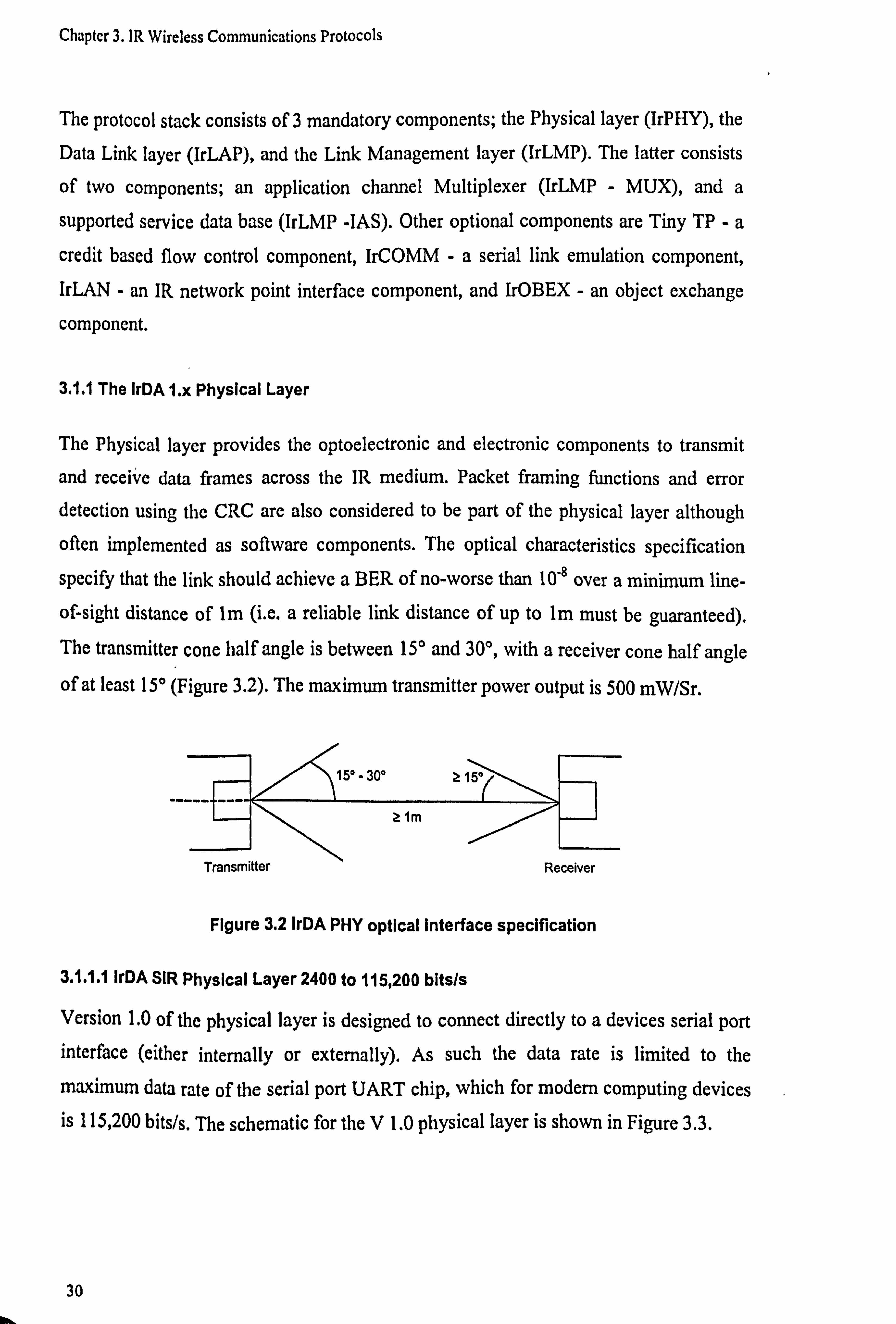
Chapter 3. IR Wireless Communications Protocols
The protocol stack consists of 3 mandatory components; the Physical layer (IrPHY), the
Data Link layer (IrLAP), and the Link Management layer (IrLMP). The latter consists
of two components; an application channel Multiplexer (IrLMP - MUX), and a
supported service data base (IrLMP -IAS). Other optional components are Tiny TP -a
credit based flow control component, IrCOMM -a serial link emulation component,
IrLAN - an IR network point interface component, and IrOBEX - an object exchange
component.
3.1.1 The IrDA 1. x Physical Layer
The Physical layer provides the optoelectronic and electronic components to transmit
and receive data frames across the IR medium. Packet framing functions and error detection using the CRC are also considered to be part of the physical layer although
often implemented as software components. The optical characteristics specification
specify that the link should achieve a BER of no-worse than 10.8 over a minimum line-
of-sight distance of lm (i. e. a reliable link distance of up to lm must be guaranteed). The transmitter cone half angle is between 15° and 30°, with a receiver cone half angle
of at least 15° (Figure 3.2). The maximum transmitter power output is 500 mW/Sr.
\ 15° - 30° Z 15°
/ L---ý 21m
Transmitter Receiver
Figure 3.2 IrDA PHY optical Interface specification
3.1.1.1 IrDA SIR Physical Layer 2400 to 115,200 bits/s
Version 1.0 of the physical layer is designed to connect directly to a devices serial port interface (either internally or externally). As such the data rate is limited to the
maximum data rate of the serial port UART chip, which for modern computing devices is 115,200 bits/s. The schematic for the V 1.0 physical layer is shown in Figure 3.3.
30
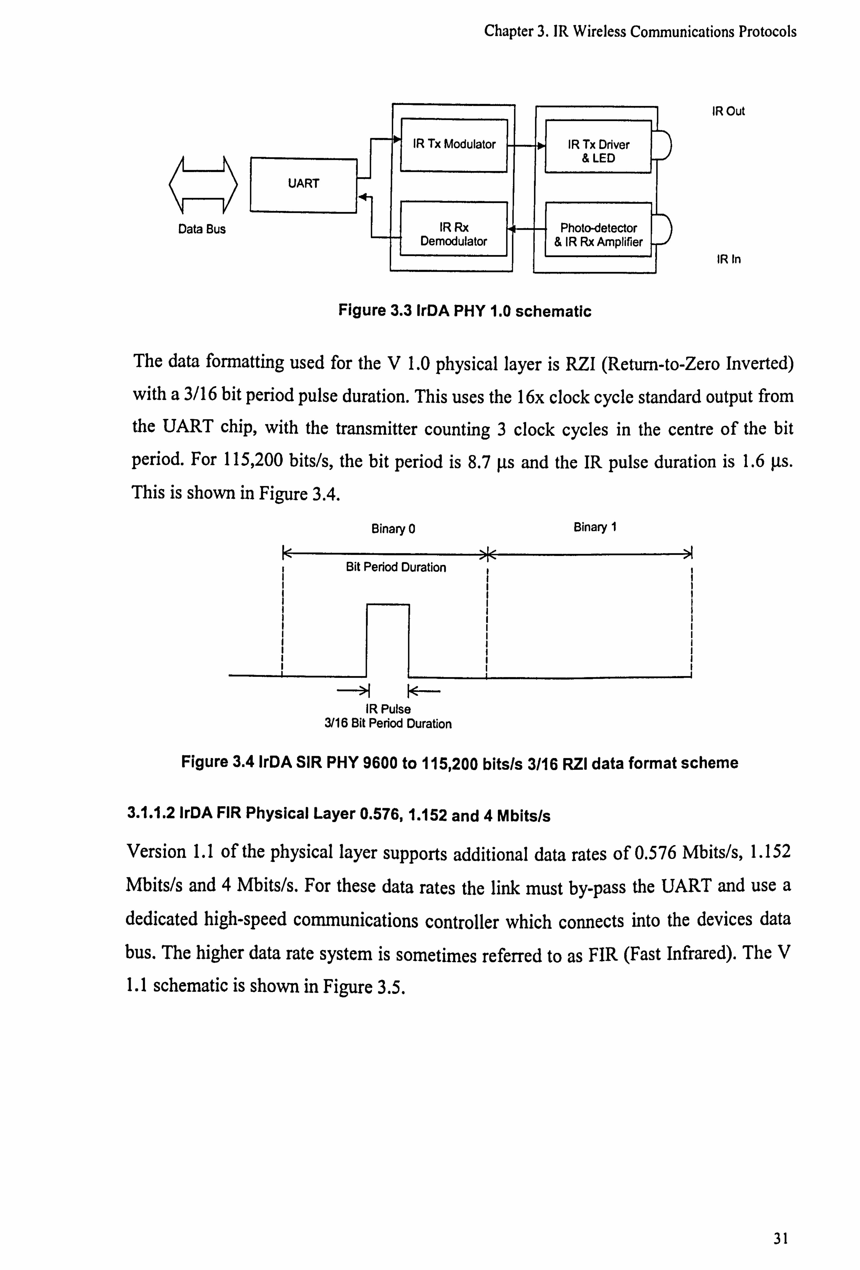
Chapter 3. JR Wireless Communications Protocols
IR Out
a Data Bus
UART
IR Tx Modulator
IR Rx Demodulator
IR Tx Driver & LED
Photo-detector & IR Rx Amplifier
IR In
Figure 3.3 IrDA PHY 1.0 schematic
The data formatting used for the V 1.0 physical layer is RZI (Return-to-Zero Inverted)
with a 3/16 bit period pulse duration. This uses the 16x clock cycle standard output from
the UART chip, with the transmitter counting 3 clock cycles in the centre of the bit
period. For 115,200 bits/s, the bit period is 8.7 µs and the IR pulse duration is 1.6 µs.
This is shown in Figure 3.4.
Binary 0
I Bit Period Duration
->i I<-- IR Pulse
3116 Bit Period Duration
Binary I
I
Figure 3.4 IrDA SIR PHY 9600 to 115,200 bits! s 3/16 RZI data format scheme
3.1.1.2 IrDA FIR Physical Layer 0.576,1.152 and 4 Mbits/s
Version 1.1 of the physical layer supports additional data rates of 0.576 Mbits/s, 1.152
Mbits/s and 4 Mbits/s. For these data rates the link must by-pass the UART and use a dedicated high-speed communications controller which connects into the devices data
bus. The higher data rate system is sometimes referred to as FIR (Fast Infrared). The V
1.1 schematic is shown in Figure 3.5.
31

Chapter 3. IR Wireless Communications Protocols
a Comms
Controller
10 9600 bits/s
to 115,200 bits/s codec
ý Transceiver module
Data Bus
N--ºI
41
L---º
0.576 81.152 Mbftsls codec
4 Mbits/s 4 PPM codec
IR Tx Driver & LED
IR Rx Amplifier & Photo-detector
Figure 3.5 IrDA PHY 1.1 schematic
IR Out
IR In
The 0.576 Mbits/s and 1.152 Mbits/s data rates use the same RZI encoding scheme as
the V 1.0 physical layer but with a 1/4 bit period pulse duration.
The 4 Mbits/s data rate uses a 4PPM modulation scheme. With 4PPM a bit-pair is
represented by a PPM symbol with 4 time slots. A single pulse positioned in each time
slot gives each of the 4 possible combinations of the 2 data bits (IrDA, 1995b), as
shown in Figure 3.6.
00
PPM Symbol
01 10 11
Figure 3.6 IrDA FIR PHY 4 Mbits/s 4PPM modulation scheme
3.1.1.3 IrDA VFIR Physical Layer 16 Mbits/s
A proposal has been made within IrDA to extend the maximum data rate of the IrDA
1. x protocol from 4 Mbits/s to 16 Mbits/s. The 16 Mbits/s VFIR (Very Fast Infrared)
extension uses a different modulation scheme to that of the 4 Mbits/s links (Petrilla,
1998). The so called HHH(1,13) modulation code - named after the developers of the
code: Walter Hirt, Martin Hassner and Nyles Heise at IBM - is a rate 2/3 (1,1315) RLL
32

Chapter 3. IR Wireless Communications Protocols
(run-length limited) code specifically developed for VFIR (Hirt et al., 2001). The
encoding provides a minimum pulse separation of 1 empty pulse slot and a maximum of
13 empty pulse slots, with a maximum of 5 consecutive minimum pulse separations.
The reason for using an RLL code is to eliminate the possibility of `back-to-back'
pulses, which can lead to intersymbol-interference (ISI) at high data rates from multi-
path propagations (Audeh and Kahn, 1995). The rate 2/3 code also has a better
bandwidth efficientcy than the 1/2 rate 4PPM encoding (Beale, 1999; Beale, 2000) .
3.1.2 The IrLAP Layer
The IrLAP layer is the data link layer of the IrDA SIR protocol stack. Its operation is
closely based on the HDLC NRM (Normal Response Mode) protocol with additional
media access functions. As such it is an `unbalanced' HDLC protocol using Primary and
Secondary station roles. Its main functions are:
" Device discovery
" Parameter negotiation
" Link establishment and role assignment
" Data transfer control
" Error recovery
" Link shut-down
" Packet formatting
The IrLAP procedural flow for connection establishment, data transfer and
disconnection are shown in Figure 3.7. Before connection can be established, device
discovery must complete during which exchange of randomly chosen 32 bit IrLAP
addresses takes place. A procedure is also available to resolve any address conflicts.
Devices then connect during which negotiation of link parameters takes place (see
section 3.1.2.2). After completion of information transfer, the link is disconnected.
33

Chapter 3. IR Wireless Communications Protocols
Inltletbn Device Discovery
Connect --0
Information Exchange
I
3.1.2.1 IrLAP Frame Format
Figure 3.7 IrLAP procedure flow
Reset
ý-0 Disconnect
The IrLAP packet consists of the Address field, the Control field, and the Information
field. The Address field contains a7 bit connection address and a C/R
(Command/Response) flag bit indicating whether the frame represents a command or
response. The Control field contains command codes and sequencing information used
for information exchange control. The Information field contains the user data packet
from the upper layer of the protocol and can have a size from 0 to 2048 bytes (16384
bits). The IrLAP packet is then encapsulated in the physical layer `wrapper' which
consists of a BOF (Beginning Of Frame) field, the FCS (Frame Checking Sequence) for
the CRC (16 bit for 9600 bits/s to 1.152 Mbits/s, 32 bit for 4 and 16 Mbits/s) and an
EOF (End Of Frame) field. This illustrated in Figure 3.8.
Address (7 bits)
BOF (8 bits)
Conflict Resolution
C/R
I
Control (8 bits)
IrLAP packet
IrLAP packet (N bits)
Information (0 to 16384 bits)
FCS (16/32 bits)
Physical layer frame
Figure 3.8 IrLAP packet format
EOF (8 bits)
34

Chapter 3. IR Wireless Communications Protocols
The FCS contains the results from a Cyclic Redundancy Check (CRC) operation. The
CRC uses the 16 bit CRC-CCITT polynomial (x16 + x12 + x5 + 1) for the data rates 9600
bits/s to 1.152 Mbits/s, while the 4 and 16 Mbits/s links use the 32 bit IEEE 802 CRC32
polynomial (x32 +x26 +x23 +x22 +x, 16 +x12 +x11 +x10 +x8 +x7 +x5 +x4 +x2 + 1)
Frames that fail the CRC are simply discarded and not passed to the IrLAP process.
The Control field identifies the frame type. As with HDLC, there are 3 frame types
used; the Unnumbered frame (U-frame), the Supervisory frame (S-frame) and the
Information frame (I-frame). The U-frame contains no sequencing information (hence
unnumbered) and is used in device discovery and connection procedures (and to
exchange data unreliably outside of an established link). The U-frame structure is as
shown in Figure 3.9 where X represents command / response code bits which are given
in Table 3.1.
76543210
X X X P/F X X 1 1
Figure 3.9 IrLAP U-frame control field
Command / Response Description Code SNRM command Set Normal Response Mode 10000 DISC command Disconnect 01000 UI command / response Unnumbered Information 00000 XID command / response Exchange Identification 00111 TEST command / response Test 11100 RNRM response Request Normal Response Mode 10000 UA response Unnumbered Acknowledgement 01100 FRMR response Frame Reject 10001 DM response Disconnected Mode 00011 RD response Request Disconnect 01000
Table 3.1 IrLAP U-frame command I response codes
S-frames are short control frames, containing no Information field, which are used in
controlling the information exchange process. The S-frame structure is shown in a
Figure 3.10 with the command / response code bits given in Table 3.2.
35

Chapter 3. IR Wireless Communications Protocols
765 Nr
432
P/F X X
I0
0 1
Figure 3.10 IrLAP S-frame control field
Command /Response Description Code RR command / response Receive Ready 00 RNR command / response Receive Not Ready 01 REJ command / response Reject 10 SREJ command / response Selective Reject 11
Table 3.2 IrLAP S-frame command I response codes
I-frames contain the user data to be exchanged and full sequencing information. The
control field structure is shown in Figure 3.11.
765
Nr
43210
P/F Ns I
1
Figure 3.11 IrLAP I-frame control field i
All frame types contain the P/F (Poll-Final) bit in the control field which is used for
station polling. For the Primary station it is referred to a the Poll bit, and for the Secondary it is the Final bit.
Ns and Nr are send and receive sequence numbers that are contained within 3 bit fields.
As such they can represent values 0 to 7. Ns fields are contained in I-frames only and
sequence unacknowledged transmitted data frames. Nr fields are contained in both I-
frames and S-frames and are used to acknowledge the receipt of I-frames. A returned Nr
value indicates that I-frames with Ns values up to and including (Nr -1) have been
successfully received (and in order), and that Nr is the next expected Ns value to be
received.
36

Chapter 3. IR Wireless Communications Protocols
3.1.2.2 IrLAP Connection Establishment
Before a link connection can be established, a device must first discover other devices
within range that it can connect to. Discovery involves exchanging the 32 bit IrLAP
device address which is randomly assigned at IrLAP initiation. In the unlikely event that
devices choose the same IrLAP address, the address conflict resolution procedure is
invoked which forces the devices to choose new addresses. A device may then connect
to one of the devices discovered. During connection establishment, parameter
negotiation takes place. All negotiation traffic takes place at the base data rate of 9600
bits/s. The link parameters involved are as follows.
Data Rate: This is the data rate at which information exchange will take place. Connecting devices must agree on the same data rate. This has a maximum value of
115,200 bits/s ,4 Mbits/s or 16 Mbits/s depending on physical layer specification.
Maximum Turnaround Time: This is the maximum time that a station can hold
transmission status before it must pass permission to transmit to the other station in the
link. This has a maximum duration of 500 ms.
Minimum Turnaround Time: This is the minimum time that the station must wait
when transferring from a receiving state to a transmission state. This delay covers for
receiver latency. This has a maximum value of 10 ms.
Maximum Data Size: This is the maximum number of data bits that can be sent in each
packet. This has a maximum value of 16384 bits (2048 bytes).
Maximum Window Size: This is the requested maximum number of frames that a
station can transmit before it must pass permission to transmit to the other station in the
link. This has a maximum value of 7 frames or 127 for the VFIR high speed extension.
The actual window size used in the link is determined by using the lesser ' of the
requested maximum window size and the window possible to transmit within the
maximum turnaround time (which has priority over the requested window size) using
the data rate, packet data size and packet overhead size.
37

Chapter 3. IR Wireless Communications Protocols
3.1.2.3 IrLAP Information Exchange Procedure
There are two principal states, receive (RECV) and transmit (XMIT). The station
resides in the XMIT state during the period it has transmission status and accepts data
transmission requests from the upper layer. The station resides in the RECV state when the other station in the connection is in the XMIT state and accepts received packets from the physical layer. The minimum turn-around delay must be implemented when
moving from the RECV state to the XMIT state. The basic IrLAP information exchange
procedure is closely based on the HDLC NRM procedure and is summarised as follows.
Each station holds a transmit sequence variable Vs, a receive sequence variable Vr, and a window variable. The window variable is initialised to the negotiated maximum window size while Vs and Vr are initialised to 0. When a data packet is to be
transmitted, a buffer copy of the data is made with index Vs. The Vs value is then
copied to the Ns field of the out-going frame. When the frame has been transmitted the Vs value is incremented by 1, and the window value is reduced by 1. If the window value becomes 1, this indicates that the next frame is the last in the sequence. Therefore
the P/F bit of the frame is set and station moves to the RECV state on transmitting the frame. The process is illustrated in Figure 3.12.
window = MaxWindow Vs=0, Vr=0
Get(data) buffer(Vs) = data
XMT(I, Vs, Vr, NOTP, data) Vs = (Vs + 1)%8
window = window -1
Get(data) buffer[Vs] = data
XMT(I, Vs, Vr, P, data) Vs = (Vs + 1)%8
window = MaxWindow
I Enter RECV State
Figure 3.12 Primary station XMIT state frame transmission procedure
38

Chapter 3. IR Wireless Communications Protocols
When a frame is received, the Ns sequence value is checked against that expected. It
should be equal to the current receive sequence variable Vr. If it is as expected, the
frame is accepted and the Vr variable is incremented by 1. If it is not as expected, this
indicates a lost frame somewhere in the sequence and that the current received frame is
out-of-sequence. The frame is then rejected and the Vr value remains unchanged. When
transmitting either an S-frame or an I-frame, the current Vr value is copied to the Nr
field of the frame. On receiving an S-frame or an I-frame with the P/F bit set the Nr
sequence value is also checked against that expected. It should be equal to the current
send sequence variable Vs (as Nr indicates the next expected frame number). If it is as
expected, the frame sequence has been successfully received and no further action is
taken except to clear buffered data that has been acknowledged. If it is not as expected,
this indicates a lost transmitted frame. The buffered data must now be re-transmitted
beginning with the sequence number indicated by Nr. If the re-transmitted frames do not
fill the full sequence window, then new data frames are transmitted to fill the window.
Figure 3.13 shows the flow chart for the Primary station frame reception procedure.
Figure 3.14 shows the flow chart for the frame re-transmission procedure.
Figure 3.13 Primary station RECV state frame reception procedure
39

Chapter 3. IR Wireless Communications Protocols
window == 1?
XMT(I, I, Vr, NOTP, buffer[i]) window = window -1
i=(I+1)%8
Yes CEnter XMIT State
XMT(I, i, Vr, P, buffer[i]) window = MaxWindow
i=(i+1)%8
Figure 3.14 Primary station frame re-transmission process
The principal difference between the primary and secondary device in the link is the use
of the P-timer and F-timer, held by the primary only. The P-timer is used to set a limit
on the time the primary station can hold transmission status when there are limited or
sporadic data packet transfer requests from the upper layer. The P-timer is thus started
upon entering the XMIT state from the RECV state. If the P-timer expires, the station
will transmit a Supervisory RR-CMD frame to poll the secondary station. The F-timer is
used to set a limit on the time the primary will wait for a return of a packet with the F-
bit set from the secondary. The F-timer is thus started upon entering the RECV state from the XMIT state. If the F-timer expires, the station will transmit a Supervisory RR-
CMD to re-poll the secondary. The F-timer can expire if the packet with the P bit set from the primary is lost, or the returning packet with the F-bit set from the secondary is
lost, or the secondary has become inactive. The secondary station does not hold P and F
timers but must reply with an F bit frame and return to the RECV state if further data
packets are not immediately waiting for transmission.
40

Chapter 3. IR Wireless Communications Protocols
Examples of IrLAP data transfer are illustrated in Figure 3.15. Data transfer from the
Primary to Secondary only is shown in sub Figure (a). The Primary transmits a window
of 7 frames from 100 (I-frame, Ns = 0, Nr = 0, P-bit not set) to 160. Here frame 130 is
lost due to bit errors (marked with an X). The Secondary responds with an S-frame with
Nr =3 acknowledging reception of frames up to and including Ns =2 (Nr -1). The
primary therefore re-transmits with I-frames starting from Ns = 3. When the re-
transmission of frames has completed, new frames starting from 170 are transmitted to
fill the window.
Two way data transfer from Primary to Secondary and Secondary to Primary is shown
sub Figure (b). As before a window of frames is transmitted with frame 130 being lost.
The Secondary now replies with its own data packets with Nr indicating acknowledged
frames. However frame 113 is also lost due to bit errors. Following the reception of the
F bit frame, the Primary re-transmits its data packets with Nr set to acknowledge the
received packets from the Secondary. The Secondary will now require to re-transmit its
own packets from Ns =1.
Sub Figure (c) shows data transfer from the Primary to Secondary only but with an F-
timer time-out. Here the P bit carrying frame 160P is lost in addition to frame 130. The
Secondary therefore does not reply with an S-frame and so the F-timer expires. The
Primary then re-polls the Secondary with an S-frame. The Secondary then replies with
its own S-frame acknowledging the received frames. The returned Nr is still 3 as this
was the first lost frame in the sequence (IrDA, 1996b).
41

Chapter 3. IR Wireless Communications Protocols
PSPS 100
110
120
I3
14
I50
I60P
S3F
Retransmission
New Packets
130
140
P150 I60
I70
100 I10P
S2F
I00
I10
120
I3
I4
I50
I60P
103
11
12
133
I43
153
163F _
131 I
141
(a) (b)
PS
100
10
20
13,0
4 i[A 150
6P ý
SOP
S3F , I30P
140P
(c)
F-timer time-out
Retransmission
Figure 3.15 Example IrLAP transfers (a) P to S data transfer (b) P to S and S to P data transfer (c) P to S data transfer with F-timer time out.
3.1.2.4 IrLAP Extension for 16 Mbits/s VFIR
The proposed extension of the maximum IrDA 1. x physical layer data rate to 16 Mbits/s
has also required a revision of the IrLAP layer to support the higher data rate. At the 16
Mbits/s rate, the frequency of link turn-around using the standard 7 frame maximum
window size and link turn-around delays would impair the efficiency of the link. An
extension to the IrLAP protocol was therefore proposed in which the maximum window
size was increased from 7 to 127 frames. This required a restructuring of the IrLAP
frame control field to increase the Nr and Ns sub-fields from 3 to 7 bits, thus requiring
an extension of the control field from 1 to 2 bytes. The additional frame overhead makes
negligible difference to the protocol throughput. However the use of the 127 frame
maximum window size can have implications for throughput with a poor BER. This is
analysed in chapter 6.
42

Chapter 3. IR Wireless Communications Protocols
3.1.3 Other IrLAP Components
The IrLMP protocol layer sits on top of the IrLAP layer and provides two distinct
services: the LM-MUX (Multiplexer) and the LM IAS (Information Access Service).
The LM-MUX is a Multiplexer that allows multiple client data applications to
communicate independently and simultaneously through a single IrLAP connection.
This is achieved through the use of a Link Service Access Point (LSAP) address
attached to the user data which will direct the data through the specified Multiplexer
channel. The LM-IAS (Information Access Service) is an object based information base
that contains information on services made available to a connecting device. Following
the claiming of an IrLMP-MUX port, a device advertises itself to the communicating
device by placing available service information and related parameters in the database
(IrDA, 1996a).
Tiny TP is an optional transport protocol which implements credit-based application-
level flow control and data segmentation and re-assembly functions. The credit-based
flow control function can overcome possible bottle-neck problems with the IrLMP
Multiplexer if a large data set is being transferred over a channel. The flow control will
ensure that only a certain amount of application data is released at a time to the
Multiplexer (IrDA, 1995c). The IrLAN component is a network interface protocol that
provides interaction with Ethernet LANs through an infrared LAN access port (IrDA,
1997a).
The IrCOMM component provides emulation of a serial cable connection between two
devices. Legacy serial application can then simply use the virtual COM ports
established with IrCOMM to exchange serial data with complete transparency to the
underlying IR architecture (IrDA, 1995a). IrCOMM supports both data-terminal-
equipment (DTE) and data-communications-equipment (DCE) connections. The
IrOBEX component is an object (e. g. business card) exchange protocol that is based
upon the HTTP protocol (IrDA, 1997b).
43

Chapter 3. IR Wireless Communications Protocols
3.2 The Advanced Infrared (Air) Protocol
The basis of the AIr protocol is to relax the physical layer restrictions of the IrDA
physical layer to provide a robust broadcast medium and to split the IrDA protocol IrLAP layer into three sub-layers consisting of the AIr MAC layer, the AIr LM (Link
Management) layer and the AIr LC (Link Control Layer).. The protocol stack is shown in Figure 3.16.
Applications
----------------------------------
IrLMP-IAS Tiny TP Legacy Transport Protocols
Application Layer
Transport/ Network Layer IrLMP-MUX
---------------------------------- AIr LC IrLAP
AIr LM
AIr MAC
802.2
---------------------------------- ATr PHY Ir PHY
Data Link Layer
Physical Layer
Figure 3.16 The Air Protocol stack
3.2.1 The Air Physical Layer
The AIr Physical Layer specifies the transceiver characteristics and modulation scheme to be used by AIr devices. In contrast to the IrDA physical layer (IrPHY) which being
used for point-to-point directed links specifies a narrow transmission cone with
maximum half angle off 15°, the AIr physical layer (AIr PHY) allows for much wider transmission angles and reception angles to provide a `broadcast' medium in which
multiple devices can communicate.
The AIr physical layer specification provides 2 classes of transceiver: standard range (S- Class) and long range (L-Class). S-Class transceivers have a radiant intensity between
60 and 150 mW/Sr which under normal lighting conditions should translate to a range
44

Chapter 3. IR Wireless Communications Protocols
between 1 and 2.5 m. L-Class transceivers have a radiant intensity of 150 to 360 mW/Sr
which gives a range of 2.5 to 6 m.
In addition to the two classes of transceiver power output, there are two classes of
transceiver half-power angle: narrow angle and wide angle. Narrow angle transceivers
have a half angle between ± 15° and ± 30°. Wide angle transceivers have a half angle
between ± 60° and ± 75° (Figure 3.17). The `half angle' refers to the angle at which the
radiant intensity falls to half that of the maximum intensity. Also for AIr transceivers,
different half angle values for the horizontal and vertical axes can be used. This allows
for a harrow beam in the vertical axis but a wide beam in the horizontal axis in
applications where devices are placed in the same horizontal plane (on a meeting table
for example) which will help conserve power.
t 15° to ± 30° (Narrow) f 60° to ± 75° (Wide)
I to 2.5 m (S-Class) 2.5 to 6m (L-Class)
Figure 3.17 Air optical interface specifications
The modulation scheme used is 4PPM with variable repetition encoding (4PPM VR)
with a base data rate of 4 Mbits/s (Figure 3.18). The basis of variable repetition
encoding is to use a variable number of repetition of each 4PPM symbol and use
majority voting on valid symbols. The principle is to provide a trade-off between
effective data rate and link quality. If chip errors occur due to noise in the link it may
(depending on the severity of the noise) only cause an error in a minority of the repeated
4PPM symbols in which case the overall symbol (representing 2 data bits) will be
accepted. This makes the link highly robust but reduces the effective data rate. In
addition, the 4PPM/VR scheme provides a variable data rate and virtual receiver
bandwidth reduction (B/RR) without any physical change to the receiver circuitry (Gfeller and Hirt, 1998).
45

l'hahtcr ( IIi Wlfl'ICSS ('0nimiUniCatilu1s I'flltl)CIIS
RR Effective Data Rate ---- SNR Gain (wrt RR =1)
1 4 Mbits/s 0 dB 2 2 Mbits/s 3 dB 4 I Mbitsis 6 dB
K 50() kbits/s 9 dB 16 25() kbits/s 12 dB
Table 3.3 Variable repetition rates with effective data rate and SNR gain
411PM Symbol RR I
I2ý4 ; lime
II II I_! -- IIII! II
4PPM Varibalc Repetition RR -4
ýI 'rime
Figure 3.18 Example variable repetition 4PPM encoding
3.2.2 The Air MAC Protocol
The Air MAC protocol is a CSMA/CA (Carrier Sensing Multiple Access with Collision
i\voidance) medium access protocol with RTS/CTS medium reservation. Although the
Air MAC specification provides a range of data delivery serv ices, including unreserved
and proxy, the following principally describes the reserved mode data transfer.
3.2.2.1 The Alr MAC Frame Structure
'l'he Air frame structure is given in figure 3.19. The Preamble (PA) and
Synchronisation (Sync) fields are used in carrier sensing, receiver synchronisation and
identii'ying the exact start of the actual frame. The robust header identifies the frame
type and carries other essential information for MAC operation. The Robust Header has
just 32 bits but is always encoded with the maximum 16 RR repetition. The Main Body
field is nut always present and can be of a variable length and with variable RR
encoding. It is primarily used to carry the payload data but can also carry addressing
40

('hahtcr ;. IIZ Wlrclcs"', ('(1nuuunications I'rutoc. uls
information in certain frame. If the Main Body is present, it is protected by a 32 bit
CRC field. The CRC used is the 802 CR('32 polynomial. If' the CRC fails, the
Main Body only is discarded while the Robust Header is still passed to the MA('
procedure.
Rol u. +tIlcadn itivcd ItH It, i
RTti
('TS
SOD
DATA. UDATA & ADA IA
SI)A lA
A('K
SPOIL
SACK
EOB
EOI3c
PA Sym RID 'iypo
PA Sync
PA lync
R'I' I RR
Riß T
Type RT
RID Type MT RR
ýmervý
rexrved
ýý(RC :] I
A, Iv kltl
it}nvn7 RIM CRC
PA Itivnc RID Type BL RR -d D. 4 SA M(1MT
ý, In e
PA I , Sy- Rt1D Typc Bl,
vn Sýnc
I
Dam C Il. INJ 1:
DA SA Icy-S MGM-ý ---__Dntn
CRC
RID Type -oral RR- mmýarl
[ PA Sync RID Type' RR «'ý IAA CRC
i�
PA tiync
I
RID TgPe Scq-R ý
RR eerved ti: \ ý'Rl'
PA Sync
PA timc
iý sI 'i' 1. )
RID Typc nsrnN
RID Type Scq"R RR -al
ý
I 11
Figure 3.19 Air MAC frame structure
There are 12 frame types specified which are given in Table 3.4.
Type Description RTS Request To Send CTS Clear To Send SOD Start of Data EOB End of Burst EOBC End of Burst Confirm DATA Reserved Data ADATA Acknowledged Reserved Data SDATA Sequenced Reserved Data UDATA Unreserved Data ACK Acknowledgement SACK Sequenced Acknowledgement SPOLL Se uenced Poll
Table 3.4 Air MAC frame types
47

Chapter 3. IR Wireless Communications Protocols
The RTS, CTS, DATA, EOB and EOBC frames are used in reserved mode data
transfer. ACK frames are used where an acknowledgement is required for each transmitted data frame. SDATA frames are used for sequencing data frames with SACK
frames used for their acknowledgement. The SPOLL frame can be used to poll the
receiving station for a SACK frame after transmitting a certain number of SDATA
frames. UDATA frames are used for unreliable data transfer outside of a reservation. The SOD frame is used to `announce' the transmission of Non-AIr modulation frames
(i. e. IrDA frames) used for coexistence purposes. Table 3.5 gives the AIr frame section lengths and transmission times.
Frame Section Length bits Transmission Time Preamble (PA) 256 64 s Synchronisation (Sync) 160 40 p Robust Header 32 128 s (RR = 16) RTS Main Body 48 12 s (RR =1 DATA Main Body 16456 (Data = 16384 bits) 4.1 ms RR =1
Table 3.5 Air frame section sizes and transmission times
3.2.2.2 Air MAC Finite State Machine '
The Finite State Machine for the AIr MAC process is shown in Figure 3.20. This has 7
states with transition conditions between the states. L1
IDLE WAR
WAR FOR DATA
Ti
WAR FOR CTS
Figure 3.20 Air MAC finite state diagram
48

Chapter 3. IR Wireless Communications Protocols
The function of each state is described as follows.
" IDLE: The process remains in this state when there is no detected activity on the
medium.
" CONTEND: The process moves to this state when contending for the medium and
remains in this state while waiting for collision avoidance slots to expire.
" WAIT FOR CTS: The process moves to this state after transmitting an RTS frame
and remains in the state while waiting for a CTS reply or for the Wait-for-CTS timer
to expire.
" WAIT FOR DATA: The process moves to this state having transmitted a CTS
frame in response to an RTS frame and remains in the state while waiting for the
first data packet or for the Wait-for-Data timer to expire.
" TRANSMIT: The process moves to this state having received a CTS frame in
response to transmitting an RTS frame and after transmitting the first data frame,
and remains in the state while transmitting further data to the target station in the
reservation.
" RECEIVE: The process moves to this state after receiving the first data frame
either when receiving data in a reservation or when `standing by' as a non-
participant in a reservation.
" IDLE WAIT: This acts as a synchronisation state by all stations upon termination
of a reservation before returning to the IDLE state
3.2.2.3 Air MAC Reserved Mode Data Transfer
The basic process for sending Reserved data can be summarised as follows. When
reserving the medium for data transmission, three main station roles are assigned. The
Requestor is the initiator of the reservation who transmits data to the Target station.
Any other station in the network is a Non participant. When in the IDLE state, if a
station ̀ hears' an RTS/CTS exchange from another station pair, the station will move to
the RECEIVE state to wait for the media to become free again. Any request for data
transmission from the upper layer should be queued until the media is free. Upon
receiving a request from the upper LM layer to reserve the medium for data
transmission, the requestor station moves to the CONTEND state and waits a number of
49

('Ii, illIritIRW irclcss ('unnnunir; ihuiis I"'Otl)COIS
Collision Avoidance t('A) time slots before transmitting an R"i'S frame addressed to the
target station. The number of Collision Avoidance Slots (CAS) used is chosen by the
IN layer and sent with a set of ('AS values as part of the reservation request. If the start
of a frame From any other contending station is received before the collision avoidance
tinier has expired, the timer is paused and resumed (from the beginning of the next time
slot) when the medium becomes free again. Having transmitted the RTS frame, the
station starts the Wait-For-CTS (WF-CTS) timer moves to the WAIT-FOR-CTS state
and waits for a ('"I'S reply from the target station. If the CTS frame is not received
bel`6rc expiration of the WF-CTS timer (if a frame collision has occurred or the device
has become unavailable, for example) a new CAS value is chosen and the collision
avoidance timer is started again. If the reservation attempt fails for a number of
successive tries, a failure is returned to the upper LM layer.
()rice the medium has been successfully reserved a burst of data packets can be
transmitted. The number' must he such that the maximum reservation time of 500ms is
not exceeded. After the first data frame has been transmitted, the requestor moves to the
XMI'I' state to continue transmitting data. Following the final data frame an EOB (End
Of Burst) frame is transmitted. Upon receiving an RTS frame, the target station replies
with a ('TS frame, starts the Wait-For-DATA (WF-DATA) timer and moves to the
WAIT-FOR-DATA state to wait for the first data packet. On receiving a CTS frame,
non-participating stations start the Wait-For-DATA-Non-participating (WF-DATAN)
timer. When the first data packet has been received both the target and non-participating
stations move to the RFCV state. Received data packets are ignored by the non-
participating station but are passed to the upper IN layer by the target station. On
sending an [OB frame, the requestor station starts the EXITI timer and moves to the
IDLI. -WAIT state to synchronise with other stations before returning to the IDLE state.
On receiving the EOB the target station replies with an EOBC frame, starts the EXIT2
timer and moves to the IDLE-WAIT state. A reservation time (RT) timer (duration
specified by the IN data request) is also used to terminate the reservation if an EOB
frame is not received within an acceptable period. A Turn-Around (TA) delay is also
implemented at each station when moving from a transmission mode to a receiving
50

('ha l) icr ;. IR WircIcss ('unuruurica tions I'n)lllcl)Is
mode to cover receiver latency. Ddault timer drrrations for the Alr MA(' process arc
given in Table 3.6.
Timer Description ---- ----- Duration CA Slot Single Collision Avoidance slot time 800 1 Guard Timer Overlapping reservations detected 40(ßs TA Tinier Receive / Transmit turn-around delay to
cover receiver latency 20O is
WF-CTS Time-out duration for CTS reply 556 s WF-DATA Time-out duration for first data frame
(Target station) 632 ps
WF-DATAN Time-out duration for first data frame (Non-participant station)
864 is
EXITI Requestor station end-of-reservation synchronisation delay
032 is
EXIT2 Target / Non-participant station end-oll reservation synchronisation delay
200 Ps
Table 3.6 Air MAC default timer durations
The reserved mode data transfer is illustrated in Figure 3.21. The other contending
station here pauses the CA timer on receiving the start of a valid RTS frame. The CA
timer is resumed on receiving a valid EOBC frame and expiration of the EXIT2 timer to
synchronise beginning of contention with other stations
CA Slots
RTS
rrn
DA7'A DATA DAl'A GULi ixiri
Source
CTS H
ý C". U1.1C ý' .
Destination
CA, Siqts pause CA timer
IE
ýýýý
detercontrnnnn
re, umc ýý (r\ Sluts
II i
-- ý 't
IF IýI ýw1
Uthct Contending Stntmn
Figure 3.21 Air MAC reserved mode data transfer process
51

('Irililci i IIZ Vdirclcss ('ounnwnicalions I'rl)(I1Cl)Is
The RTS/('"I"S exchange involved in establishing the reservation effectively deals with
the `hidden node' problem. A hidden node (' is one which is out of range of a
transmitting station :f but which is within range of a receiving station B. By using the
R'l'S/( "I'S exchange the station (' will not receive the RTS transmission from station A
but will receive the ("I'S reply from station B (Figure 3.22). As the CTS reply also
contains the requested reservation time, station C will know to defer any transmission
until the reservation time has completed or the EOBC reply from station B is received.
The ('A slot time employed, specified as 800 µs, is chosen to deal with hidden nodes as
it is long enough to cover an RTS transmission, a turn-around delay and the beginning
(PA I SYNC) of a ("1'S reply. If the RTS initiator is hidden from a receiving station, it
can still receive start of the ('"1'S reply and pause its own CA timer before possible
transmission in the next slot. The slot time is thus constrained by:
T%Lu > %h'1: 1
+7ru +7l", +
424* µs f 200 ps f- 64 µs + 40 µs 728 µs
* using the maximum 16 RR for the RTS main body.
footprint C
i" 'ý ýý \ ý'\
.ý ý" _ýý>týý_ \
ý __. --- , ,- . ý, rý .ý i , _-' , i -' -' iý ý LJ 'ýýý ýý<ýý ýi ýý iý i ý
ýý ý
,ýý ýýi ý ><' ýý \'ý ýý ý
., 'i
_,, ýý ýýi
IL.. _1 -' I ;,
- ''_',,,. R
/ý L,
ý ýý- ý
/ýý ýýýý
I
footprint A
Figure 3.22 The hidden node problem
It is also possible to transmit in Reserved mode using acknowledgements. In this case
AI )A'I'A (Acknowledgement DATA) frames are transmitted and each frame must be
acknowledged with an ACK frame returned from the destination station (Figure 3.23 b).
If' the A('K is not returned within an acceptable period, determined by the WFACK
52

('hahtcr ;. IR Wirclcss Con III iunicatiouls I'rl)tucl)Is
(Wait For ACK) timer the reservation is terminated by sending ºn 1,; 0I3 frame.
Sequenced data can also be transmitted using SDA'I'A (Sequenced DATA) frames.
These contain sequence numbers contained in the Seq-S field. The frames are
acknowledged by the returned EOBC frame from the destination station with a received
sequenced number in the Seq-R field. As with the lrl, AP protocol the receive sequenced
number indicates the next expected send sequence number (Figure 3.23 c). Another
method of data transfer in the reserved mode is sequenced polling for reliable niulticast.
With this, a sequence of SDATA frames is transmitted with a multicast address (i. e. the
frames are received by all stations). The station then polls each station in turn using the
SPOLL (Sequenced Poll) frame and waits for each station to return a sequenced
acknowledgement (SACK) frame that acknowledges the received sequence frames
(Figure 3.23 d). The transmitting of sequenced dames allows a certain level of reliable
data transmission at the MAC' layer but the exact process for error recovery is not fully
developed in the specification.
Source Destination Source I)cst nation Source
Itlti
C'I'S
DATA
DATA
DATA
FOB
EOB('
Nrti
(, Is
AI)ATA
ACK
VI)ATA
ACK
_. ----"" f^F; OF3 ___
I. O13l'
It---"
(a) (b)
izrti
I )vstwauuQ Source
('I tiýyl
SUATAO
SIh11: ýI
tiUAIA4
FcHl
rt,
m, 4-__
(t)
I h"stutauun
(d)
Figure 3.23 Air MAC reserved mode transfer methods (a) standard reserved data transfer (h) reserved data transfer with acknowledge inent (c) reserved
sequenced data transfer (d) reserved reliable multicast data transfer
3.2.2.4 Air MAC Unreserved, Announced and Proxy Modes
The Alr MAC can also operate in Unreserved mode. Here the station will still carry out
carrier sensing and collision avoidance procedures as before but when contention is won
will transmit a single UDATA frame with no acknowledgement ti-0111 the receiver. 11'a
packet collision occurs due to two or more stations choosing the same time slot, it will
53

Chapter 3. IR Wireless Communications Protocols
be the responsibility of upper protocol layers to instigate error recovery. This is
obviously a more unreliable method of data transfer than using the RTS/CTS media
reservation. It should also be noted that as there is no acknowledgement of a transmitted
UDATA packet and it is therefore not possible for the transmitting station to determine
if a collision has occurred (Figure 3.24 a).
Other possible modes of operation for the AIr MAC are the Announced and Proxy
modes. With the Announced mode, an RTS frame is transmitted prior to transmitting a burst of data packets which is terminated by transmitting an EOB frame. However there is no acknowledgement (CTS or EOBC) from the receiving station. This provides less
of an overhead than the full reserved mode but is less reliable as there is no
confirmation of the receipt of data and the hidden node problem is not addressed (Figure
3.24 c).
The Proxy mode is used to transmit data using non-AIr modulation. This is used to
support coexistence with other IR Wireless modulation schemes and is primarily aimed
at supporting AIr - IrDA interaction. In both cases the SOD (Start Of Data) frame is
used to initiate transfer of the non-AIr modulation data. The R/M field of the SOD
frame is used to indicate the modulation scheme and data rate being employed. The MT (Modulation time) field in the SOD header indicates the expected length of time that the indicated modulation scheme will be employed (Figure 3.24 d).
Source Destination Source Destination Source Destination Source Destination
UDATA RTS
CTS
DATA
RTS
_ SOD
RTS
DATA
DATA
EOB
EOBC
(a)
Data Transmit
6os
(b) (c)
Figure 3.24 Air MAC data transfer modes. (a) Unreserved, (b) Reserved, (c) Announced, (d) Proxy.
CTS
r- SOD
__ý
Data Transmit
E0B
EOBC
(d)
54

Chapter 3. IR Wireless Communications Protocols
3.2.3 The Air LM Layer
The AIr LM (Link Management) layer is the upper layer client for the AIr MAC. The
LM provides multiplexing for different LC (Link Control) clients in addition to
providing support for GroupWare services, reliable, unreliable and priority data
delivery, coexistence services (with the IrDA protocol) and adaptive data rates. In
requesting a reservation from the AIr MAC it is the responsibility of the LM to define
the set of CAS (Collision Avoidance Slot) values to be used by the MAC. The values
are sent to the MAC as a CAS vector where the index is the current reservation retry-
count. The CAS values are chosen randomly from a range of possible values called the
`CAS window' (i. e. from 0 to W-1) which becomes a input parameter to the system. A
minimum CAS window value of 8 slots is specified. It can be seen that the larger the
CAS window the less likely that 2 or more stations will choose the same CAS value and
cause an RTS collision. However a large CAS value will cause an excessive time
overhead in reserving the medium. Therefore a linear CAS back-off algorithm is
provided in the specification in which the CAS window size is increased (with an upper
limit) for the next retry following a failed reservation attempt, and decreased (with a
lower limit) following a successful reservation (Figure 3.25). The specification advises
an minimum CAS window increment of 4 slots, and a maximum CAS window
decrement of 4 slots with a lower CAS limit of 8 slots and an upper CAS limit of 256
slots. This is illustrated in figure 3.25 where a is the CAS window increase adjustment
for a successful reservation and b is the CAS window decrease for a reservation failure.
window = min window
Figure 3.25 Air LM CAS back-off process
55

Chapter 3. IR Wireless Communications Protocols
The LM is also responsible for supplying other reservation parameters to the MAC layer
such as the Repetition Rate (RR) to be used, the required reservation time, and the retry limit (IrDA, 1999c).
3.2.4 The Air LC Layer
The AIr LC (Link Control) layer is a HDLC based data link protocol. As such it can be
seen as replacement for the reliable data delivery functions of the IrLAP protocol. However the AIr LC protocol uses balanced stations (i. e. there are no primary /
secondary roles) and as such is based on HDLC ABM (Asynchronous Balanced Mode)
as opposed to the NRM based IrLAP protocol. However the error recovery procedure
uses Ns and Ns sequence fields and operates in the same manner as described for the IrLAP protocol. The specification for the LC protocol is currently in a draft state and the
exact method of interaction with the lower protocols is not yet fully developed (IrDA,
1999b).
3.3 Chapter Summary
This chapter has described in detail the two IR wireless protocol standards whose performance is investigated in this thesis. The IrDA 1. x protocol is described with emphasis on the IR PHY layer, and the IrLAP data link layer information exchange procedure. The functions of the upper layer in the protocol set and the proposed high
speed (16 Mbits/s) extension are also summarised. The Advanced Infrared (AIr)
protocol which is a development of the IrDA protocol to provide a multiple access IR `network' is described with emphasis on the AIr PHY layer and AIr MAC layer. The following chapter provides and analytical model of the IR wireless physical layer
relating bit-error-rate (BER) to transceiver characteristics, link geometry and noise source levels. Third user interference and resulting asymmetry effects are also examined.
56

4. PHYSICAL LAYER ANALYSIS
This chapter examines physical layer properties of IR wireless links to highlight the
critical physical layer factors affecting performance and provides expressions for the
bit-error-rate (BER) and packet error probabilities of links. The BER at the receiver is
derived from the receiver electrical signal-to-noise ratio (SNR) and the line encoding
and detection scheme employed. The SNR is dependent on the transceiver
characteristics, link geometry and receiver noise levels. The effects of third user
interference and resultant link asymmetry are also examined.
4.1 IR Channel Model
We assume in this model a directed LOS link with no multipath propagation. The
characteristics of non-directed channels have been modelled elsewhere (Barry et al.,
1991b; Carruthers and Kahn, 1997; Florez et al., 1997; Jungnickel et al., 2002; Samaras
et al., 1998). Other assumptions are made during the course of the analysis. We assume
that an IR wireless link employing an LED transmitter and PIN photodiode receiver
uses intensity modulation with direct detection (IM/DD). Figure 4.1 shows the IR
wireless IM/DD transmission and reception model. The LED output power PT (Watts) is
modulated by the signal waveform u(t) giving the transmitted signal X(t). This is
convoluted with the channel impulse response h(t) and the receiver responsivity R
(Amps / Watts) and is added to the receiver noise signal N(t) to produce the output
photocurrent signal Y(t).
Signal Waveform u(t) Transmitted Received Signal
Vbins PIN Photodiode
Signal X(t) Power PR Responsivity R
-Zý Channel Noise Current N(t)
Impulse Response h(t)
Photo Current Y(t)
Figure 4.1 IM/DD transmission and reception model
57

ý'hahtcr I. I'Iwsic; il Laver Analysis
I'hc channel model can he represented by the schematic in Figure 4.2.
Optical Power X(t)
Photocurrent Y(t)
Noise N(t)
Figure 4.2 IR Wireless channel model
Thus the system output photocurrent Y(t) can be given by:
Y(1) K. Y(1)(x)h(1)+N(1) (4.1)
where O denotes `convolution' anti A(1) Piir(1).
The frequency response //(/) of'the channel can be given by the Fourier transform of the
channel iinpulse response h(1).
ll f /) ýlr(t )ýý '' tit (4.2)
The received optical power Pal is determined from the channel dc response H(O) by:
/',; _ //(())/I
The electrical peak signal-to-noise ratio (SNR) is then given by:
(1kR) _
(R11(0)P, )-' . SNIl -= N�B NOB
(4.3)
(4.4)
where N� is the double-sided noise power spectral density (A2/Hz), assuming an
independent white Gaussian dominated noise signal N(t), and B is the receiver electrical
handwidth (II/).
5's
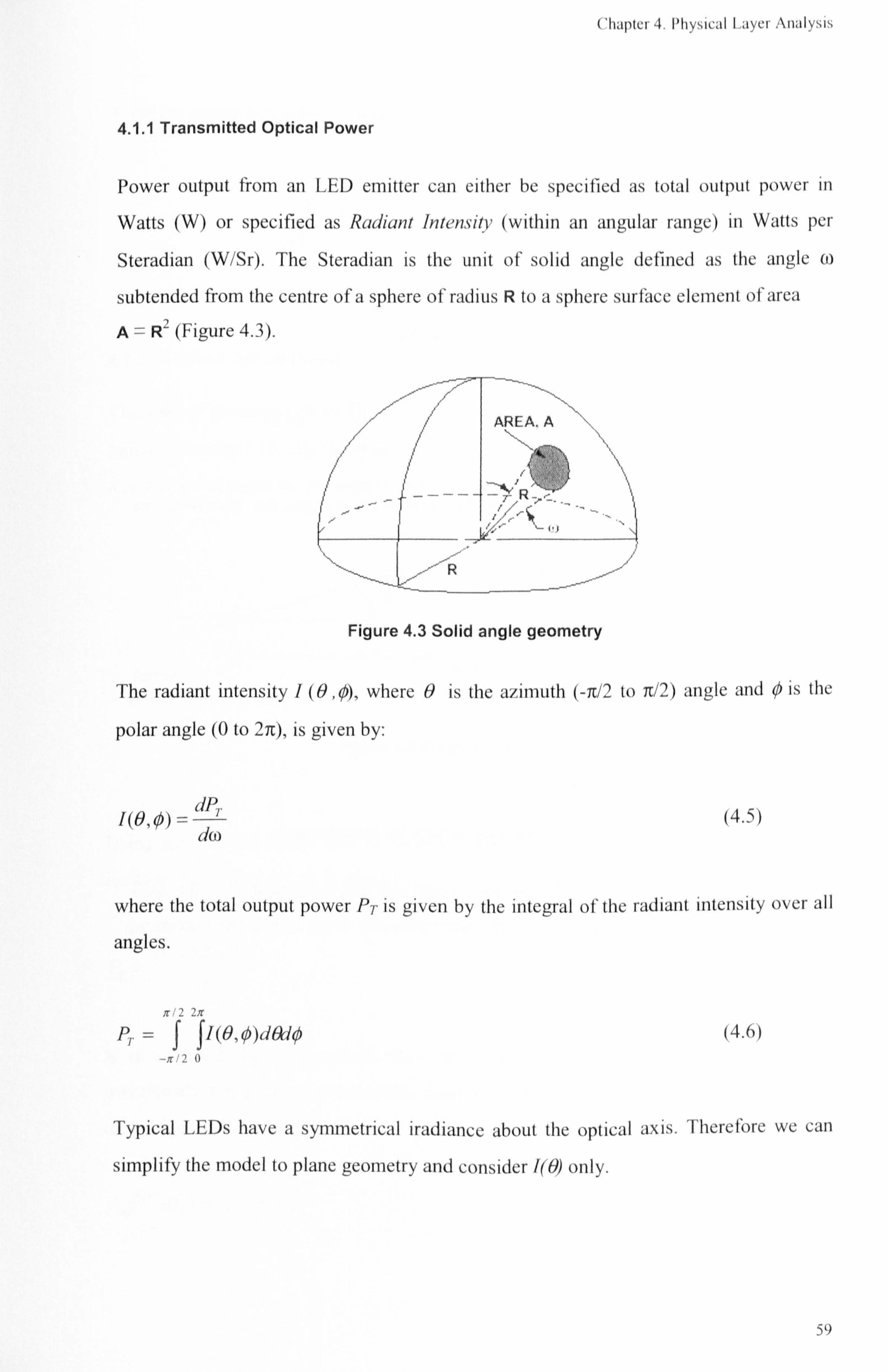
('hahlcr 4. Physical I . iycr ; \nalysis
4.1.1 Transmitted Optical Power
Power output from an LED emitter can either he specified as total output power in
Watts (W) or specified as Radiant Intensity (within an angular range) in Watts per
Steradian (W/Sr). The Steradian is the unit of solid angle defined as the angle aw
subtended from the centre of a sphere of radius R to a sphere surface element of area
A= R2 (Figure 4.3).
Figure 4.3 Solid angle geometry
The radiant intensity 1 (6 , 0), where 0 is the azimuth (-1t/2 to n/2) angle and 0 is the
polar angle (0 to 2it), is given by:
I(e, 0) = dc) (4.5)
where the total output power PT is given by the integral of the radiant intensity over all
angles.
Rr1 , 1r
f J1(Ocb)dfkiý -ir! 2 0
(4.6)
Typical LEDs have a symmetrical iradiance about the optical axis. Therefore we can
simplify the model to plane geometry and consider /(0) only.
59

I li, ihlci 4 I'Iivtiira) I . aYer An, ilvsis
Modelling the LF. I) using the general Lambert cosine law (Gfeller and Bapst, 1979)
givcti:
/JO). -- J/,, cos" H-irl 2< H S7r/ 2
I 7t/2<0<-7[12
where /� is the axial radiant intensity (at 0= 0) given by:
ý (iý + /) I)
ý, ý- 2ir
(4.7)
(4.8)
and n is the , nnclc' inr/c'. v of the radiation lobe. The higher the n value, the `narrower' the
radiation lobe becomes (Figure 4.4).
nI
n-5
n=20 \
Figure 4.4 Radiant intensity pattern for increasing n
"I'hc extent of the `narrowness' of the radiation beam can also be indicated by the half-
power angle, which is the angle at which the beam intensity drops to half the maximum intensity, given by:
N0 ,- COS 1 (0.5' ") (4.9)
60

('banter 4. Physical Layer Analysis
Table 4.1 shows the required mode index values for typical IR LED hall-power angles.
Half Power Angle (deyýrees Mode Index -n 60 1 30 5 15 20
Table 4.1 Mode index values for typical LEDs
4.1.2 Received Optical Power
The optical geometry of an IR link is shown in Figure 4.5, where the transmitter of
radiant intensity I(0), aligned at an angle 8T, and the receiver of effective detection area
A, 11 aligned at angle OR, are separated by a distance cl.
.1\
Source Radient Intensity 1(87)
Cl
Detector Effective Area
Figure 4.5 Optical link geometry
Using the inverse square law of radiation, the received optical power P,?, assuming
isotropic radiation (n =- 1), is given by:
(4.10)
It is assumed that any optical filter fitted has 100°40 transmittance at the signal
wavelength. For a bare (i. e. unlensed) detector of area A, the effective area is given by
the cosine of the incident angle.
Ajihure(aR) =ACOS(OR) (4.11)
Detector Effective Area
61
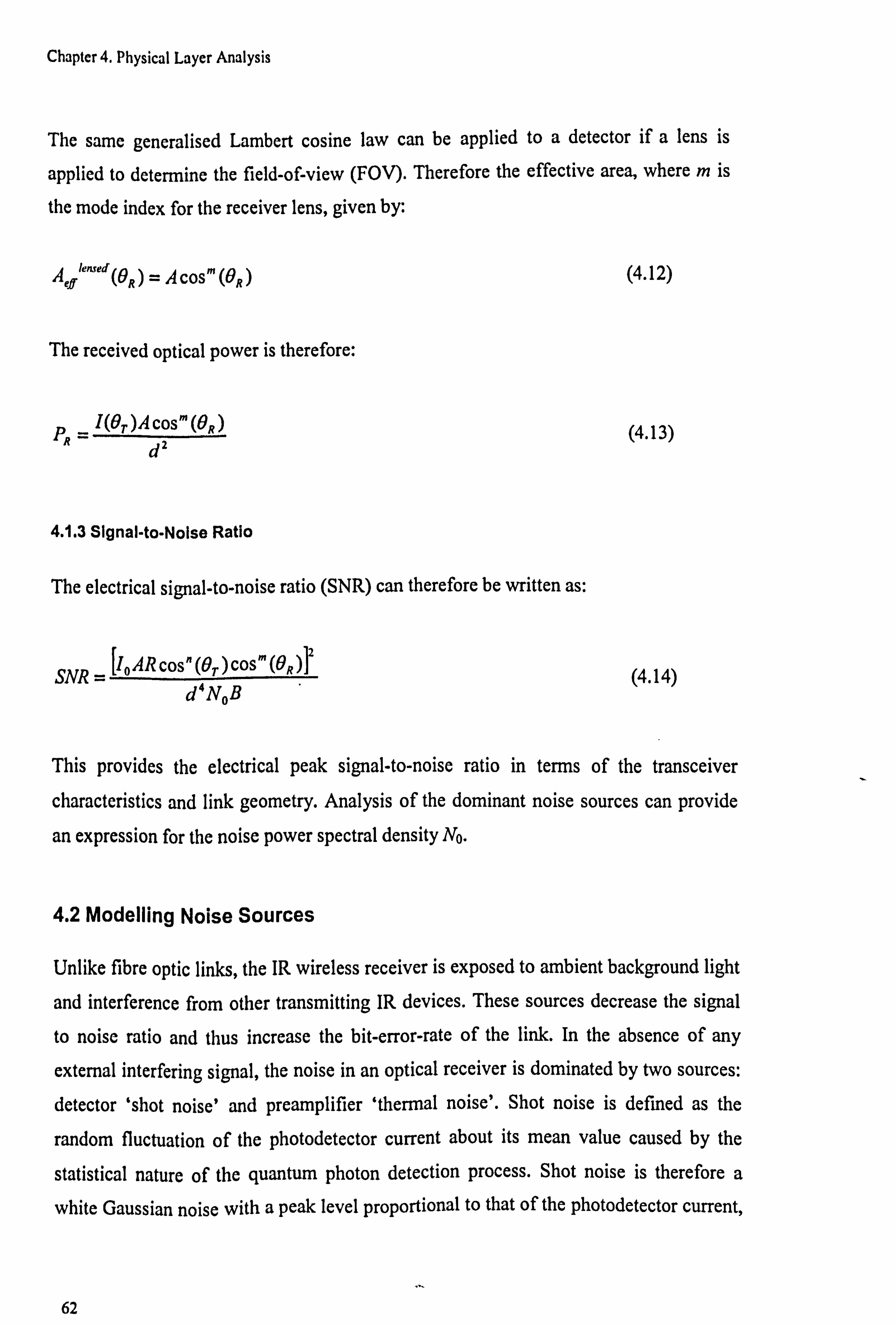
Chapter 4. Physical Layer Analysis
The same generalised Lambert cosine law can be applied to a detector if a lens is
applied to determine the field-of-view (FOV). Therefore the effective area, where m is
the mode index for the receiver lens, given by:
Ae$lensed (eR )= fi cos' (BR )
The received optical power is therefore:
Pn_ _R d2
4.1.3 Signal-to-Noise Ratio
The electrical signal-to-noise ratio (SNR) can therefore be written as:
[IOARCOS? 1(OT)COSm(OR)]2 SNR = d4NoB
(4.12)
(4.13)
(4.14)
This provides the electrical peak signal-to-noise ratio in terms of the transceiver
characteristics and link geometry. Analysis of the dominant noise sources can provide
an expression for the noise power spectral density No.
4.2 Modelling Noise Sources
Unlike fibre optic links, the IR wireless receiver is exposed to ambient background light
and interference from other transmitting IR devices. These sources decrease the signal
to noise ratio and thus increase the bit-error-rate of the link. In the absence of any
external interfering signal, the noise in an optical receiver is dominated by two sources: detector ̀ shot noise' and preamplifier `thermal noise'. Shot noise is defined as the
random fluctuation of the photodetector current about its mean value caused by the
statistical nature of the quantum photon detection process. Shot noise is therefore a
white Gaussian noise with a peak level proportional to that of the photodetector current,
I(97. )Acos'"(OR)
62

Chapter 4. Physical Layer Analysis
and therefore to the level of the incident optical power. Shot noise is produced as a
result of both the optical signal and the background ambient light but is normally
dominated by the from ambient light. Thermal noise is caused by the thermal agitation
of electrons in the carrier. This can also be considered as a white Gaussian noise. The
total double-sided power spectral density No is therefore given by:
NO Nshot + Nthermal
4.2.1 Ambient Light Induced Shot Noise
(4.15)
From Gaussian statistics, the double-sided power spectral density Nshor (A2/Hz) for shot
noise is given by
Nshor = 29jd, ý
(4.16)
where q is the electron charge (- 1.6 x 10⁻¹⁹ C) and Ids is the total photodetector dc
current which is given by:
Id= R(PR + PB ) (4.17)
where PR is the average received optical power from the IR signal and PB is the received
background ambient light optical power. If we assume that the ambient light power is
much greater than the signal power (PB» PR), then the dc current can be given by:
Ia=RPB =RAEB (4.18)
where A is the receiver area and EB is the background ambient iradiance (W/m2). This
assumes that the ambient light power is constant. This is the case with natural sunlight
(direct and indirect). For artificial light, possible interference from modulation of the
source (e. g. from electronic ballast or the AC mains frequency) may need to be taken
into consideration (Moreira et al., 1996). The spatial distribution of ambient light is
assumed to be uniform although this may often not be true for real environments
63

Chapter 4. Physical Layer Analysis
(Bakalidis et al., 1996). Typical sources of ambient light in an office or home
environment are:
" Direct sunlight
" Indirect sunlight
" Incandescent lamps (i. e. filament bulbs)
" Halogen lamps
" Fluorescent light with conventional ballast (CB)
" Fluorescent light with electronic ballast (EB)
I
0
Figure 4.6 Normalised power spectra for ambient light sources (after Kahn & Barry, 1997)
Figure 4.6 shows normalised power spectra of typical ambient light sources. It should be noted that the powers are normalised so that each has the same maximum power. In
reality, sunlight power will greatly exceed other sources. Low cost silicon photodiodes have a maximum response in the 800 to 900 nm range (see Figure 2.2). It can be seen from Figure 4.6 that incandescent lamps have a peak presence in this region. Experimental ambient iradiance values for different light sources including sunlight, incandescent lamps, and florescent lighting both with and without optical filters, are
provided by Moreira (1997). The values vary from 10 mW/cm2 for direct sunlight, to
4.3 tW/cm2 for a 13 W fluorescent lamp with conventional ballast. The IrDA test
guidelines specify a background iradiance no greater than 490 RW/cm2 for correct
operation of links.
64

Chapter 4. Physical Layer Analysis
4.2.2 Thermal Noise
In an optical receiver, the photodiode is typically followed by a transimpedance
preamplifier which converts the input current into an output voltage. These are used as
they provide a wide bandwidth and large dynamic range. Figure 4.7 shows a basic
transimpedance preamplifier receiver design.
Figure 4.7 Basic transimpedance receiver preamplifier design
The use of a high pass input filter (capacitor CI) reduces the dc level in the receiver
from ambient light (the shot noise is from the white Gaussian random fluctuations about
the mean value).
The dominant current in the receiver is that in the feedback resistor RF. The double-
sided power spectral density Nrhermal (A2/Hz) for thermal noise is therefore given by:
Nrhermnr 2kTK -R
F (4.19)
where k is the Boltzman constant (-1.38 x 10⁻²³ J/K), and TK is the absolute temperature.
It can be seen that the noise power is inversely proportional to the feedback resistance
65

Chapter 4. Physical Layer Analysis
of the amplifier. Thus the noise is easily reduced by increasing the resistance. However
this can reduce the bandwidth of the amplifier, given by:
B= 1+Ag RFC,.
(4.20)
where Ag is the amplifier voltage gain, and CT (= Cpd + C1) is the total input capacitance (Phang and Johns, 1999). The resistance RF must therefore be set such that the thermal
noise is minimised but with sufficient amplifier bandwidth for the intended bit rate. It
can be seen that the bandwidth is inversely proportional to the input capacitance. The
photodiode capacitance Cpd is proportional to the detector area A. This should therefore be minimised while obtaining sufficient optical power to maintain a required SNR.
Minimising A also reduces the level of incident ambient light power.
The careful design of IR receivers normally makes thermal noise negligible. The total
noise can be assumed to be dominated by that from the ambient light induced shot
noise. Therefore the total double sided noise power spectral density No is given by:
No = 2gIdý = 2gRAEB .
The total expression for SNR can then be written as:
SNR = RA[I0 cos" (Or) cos'" (OR) ]2
2d 4gEBB
(4.21)
(4.22)
This provides the electrical peak signal-to-noise ratio in terms of the transceiver
characteristics (transmitter radiant intensity to and lens mode index n, receiver area A,
responsivity R, lens mode index m and bandwidth B), link geometry (transmitter
alignment Or, receiver alignment 6K and link LOS distance d) and ambient light
iradiance E.
66
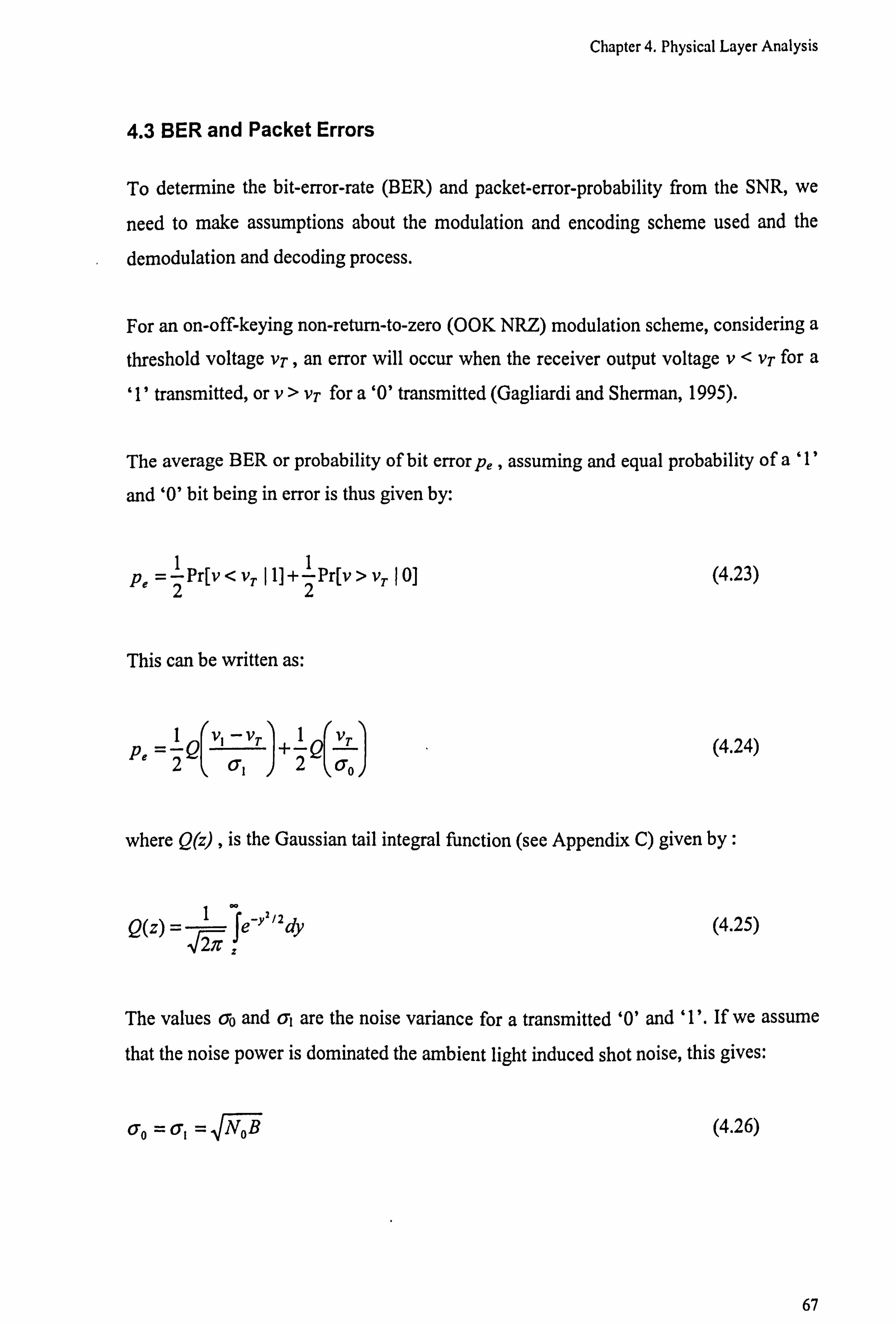
Chapter 4. Physical Layer Analysis
4.3 BER and Packet Errors
To determine the bit-error-rate (BER) and packet-error-probability from the SNR, we
need to make assumptions about the modulation and encoding scheme used and the
demodulation and decoding process.
For an on-off-keying non-return-to-zero (OOK NRZ) modulation scheme, considering a
threshold voltage vT, an error will occur when the receiver output voltage v< vT for a
`1' transmitted, or v> VT for a ̀ 0' transmitted (Gagliardi and Sherman, 1995).
The average BER or probability of bit error pe , assuming and equal probability of a `1'
and `0' bit being in error is thus given by:
Pe =2 Pr[v < vT 11] +ý Pr[v > vT 101
This can be written as:
1 vý - VT 1 v,. Pe =-Q +Q
2 61 2 CO
(4.23)
(4.24)
where Q(z) , is the Gaussian tail integral function (see Appendix C) given by:
Q(z) =1f e_yz izdY Ir _
(4.25)
The values o'o and 61 are the noise variance for a transmitted 10' and ̀ 1'. If we assume
that the noise power is dominated the ambient light induced shot noise, this gives:
co = Q, = NOB (4.26)
67

Chapter 4. Physical Layer Analysis
The BER is minimised by choosing the threshold vT to be half the received signal level
(i. e. VT: '- v1/2). Applying this to equation (4.24) gives
I VI 24-NOB
(4.27) rv, Pý_Q
2r
If the voltage vl is produced from a signal current RPR, this provides pe in relation to the
electrical peak SNR of.
pe = Q( SNR / 2) (4.28)
The packet capture probability pp, and packet error probability pp, for a data length 1 bits
are then:
pý =(1-p. )'
pp, =1- (1- pý )ý
(4.29)
(4.30)
By using an adaptive threshold where the comparator reference input is set to half the
maximum received signal voltage level the bit-error-rate can minimised (Ananth et al., 1997; Otte et al., 1999).
4.3.1 Required Bandwidth
The electrical bandwidth B of the receiver needs to be sufficiently large to correctly
receive transmitted pulses at the maximum link data rate and encoding scheme
employed. However, increasing the bandwidth increases the total noise power (from the dominant ̀ white' shot noise) and hence reduces the signal-to-noise ratio and so should be no larger than required. An approximate upper limited on the bandwidth is obtained from the inverse of the transmitted pulse duration TP.
68

Chapter 4. Physical Layer Analysis
Breq ~1 Tp (4.31)
However depending on the data rate, modulation or encoding scheme employed and the
receiver design, the bandwidth can be made smaller than that calculated and still
correctly receive transmitted pulses. The recommended bandwidth can be obtained from
the transfer function G(f) of the receiver filter and amplifier circuitry (Hirt et al., 2001).
4.3.2 IrDA SIR RZI Modulation
IrDA links up to 1.152 Mbits/s do not use NRZ modulation but RZI (Return-to-Zero
Inverted) modulation with a 3/16 bit period pulse width for up to 115.2 kbits/s and 1/4
bit period pulse width for 1.152 Mbits/s. Using a shorter pulse duration reduces the
average power requirement for the link. This also insures that a long string of zeros is
not lost in the transmission. However this also increases the bandwidth requirement
which will increase the noise power level at the receiver. The transmitted pulse is
counted for 3 clock cycles (4 for 1/4 RZI) and transmitted in the middle of the bit
period. The rising edge of the received pulse (above receiver threshold) triggers the
receiver to count 16 clock cycles during which a zero level output is produced. If no
following rising edge is detected, a ̀ 1' output is produced for a count of 16 clock cycles.
This is demonstrated in Figure 4.9 (Agilent, 2000).
16 Clock
I_ I. ycles
16x Cbck
IrTXD
I
TXCiI
-. 3 cs rt-;
mumm IUII
16x Clack
IrRXD
RXD
16 Clock i yclsý
= 3
Jt CS
n im
Figure 4.8 IrDA SIR 3/16 RZI transmission and detection
ul uUul
The same BER analysis for NRZ OOK using the peak electrical SNR can be used for
RZI. The difference is in the average power requirement Preq and bandwidth
requirement Brey. There are given by (4.33) and (4.34) for 3/16 and 1/4 RZI respectively
where Rb is the line data rate (Barry, 1994).
69

Chapter 4. Physical Layer Analysis
pp(Az, ) _ Q( SNR / 2)
Preq(3/16RZ! ) =3 32 PT andPreg(1/4RZ/) =18 Pr
Breq(3/16RTJ) 16 =3 Rb and Breq(U4RZI)
= 4Rb
4.3.3 FIR 4MbIts/s 4PPM Modulation
(4.32)
(4.33)
(4.34)
For PPM modulation, determination of the actual data bit-error-rate is a bit more difficult as for 4PPM, each symbol represents 2 data bits. Therefore it is generally easier to determine the error probability of an individual pulse or `chip', the chip-error-
probability.
Po -Q vI
11N0B
Xo -Q N-oB ' V
Assuming vT = vl/2, for 4PPM this gives:
Pcl = P, o = Q( SNR / 2)
For 4PPM, the symbol capture probability, assuming pct = pcO = pc, is:
Pic = (t-Pel)(1-Pco)3 = (1-Pc)4
which gives a packet error probability (for 1 data bits) of.
Ppe P. 1/2 =1-(1-Pc)2'
70
(4.35)
(4.36)
(4.37)
(4.38)
(4.39)

Chapter 4. Physical Layer Analysis
This provides a derived bit-error-rate p, of:
Pe(4ppm) =1' T'
=1'(1--x)Z (4.40)
The average power requirement and bandwidth requirement for 4 PPM are given by:
Preq(4ppm) 4 PT
B+'e4(4PPm) - 2R6
4.3.4 VFIR 16 Mbits/s Rate 2/3 (1,13 15) RLL HHH Encoding
(4.41)
(4.42)
From the complexity of the rate 2/3 (1,13 15) HHH encoding used for the 16 Mbits/s
VFIR physical layer (see section 3.1.1.3), it can be difficult to accurately determine the
bit-error-probability. However if we assume an equal error probability for pulse and non
pulse slots, again assuming vT = vl/2, the chip error probability is:
pe = Q( SNR / 2) (4.43)
As the coding rate produces 3 chips for every 2 data bits, the packet-error probability
can be given as:
Ppe =1-(1_Pc)3U/2 (4.44)
providing a derived bit-error-rate
3/2 Pe(HHH) =1- (1- pc) (4.45)
71

Chapter 4. Physical Layer Analysis
The average duty cycle for HHH encoding is given by Hirt et. al. (Hirt et al., 2001) as
0.258, giving an average power requirement of:
P. eq(HHH) = (0"258)Pr
The required bandwidth for the 3/2 rate encoding is:
Breq(HHH) 32
Rb
(4.46)
(4.47)
Table 4.2 provides the BER expressions, power requirements, calculated bandwidth and
recommended bandwidth for IrDA * 1. x data rates and modulation / encoding schemes.
Data Rate Range
Modulation / Encodin
Average Power Requirement
BER Calculated Bandwidth
Recommended Bandwidth
9600 -115,200 bits/s
3/16 RZI (3/32) Pr Q( SNR /2) 615 KHz 250 KHz
0.576 & 1.152 Mbits/s
1/4 RZI (1/8) Pr Q( SNR /2) 4.6 MHz 2.48 MHz
4Mbids 4PPM (1/4) Pr 1-(1-Q( SNR/2))' 8MHz 6.1 MHz
16 Mbit/s 111111 (0.258) Pr 1-(1-Q( SNR /2))'ý2 24 MHz 14.5 MHz
Table 4.2 BER expressions power requirements and bandwidth requirements for IrDA modulation / encoding schemes
Figure 4.10 shows BER versus SNR (electrical - dB) for RZI, 4PPM and HHH
modulation schemes. It can be seen that performance depends on the coding efficiency
of the modulation code with RZI having an efficiency of 1,4PPM an efficiency of 1/2
and HHH an efficiency of 2/3. It is seen that an SNR of around 21 dB is required to
achieve the minimum specified BER of 10"8 over 1 m. Figure 4.11 shows packet capture
probability, from (4.29), for 1= 2 Kbytes (16384 bits) versus SNR. It can be seen that
there is an effective zero probability of packet capture below an SNR of 16.5 dB.
72

Chapter 4. Physical Layer Analysis
0: w m
100
10 .1
102
0
10
10
i
_``==ý`_ ý
16-1 ý
10°L 0
ý= . I I
IN I
v
RZI -- 4PPM
--- HHH
I ý11
10
ý
5 10 15 20 25 SNR (dB)
Figure 4.8 BER versus SNR for IrDA modulation schemes
I
0.9
0.8
w 0.7 12 ro e 0.6 a 0 0.5
ro U 0.4 w
0.3
0.2
0.1
16 16.5 17 17.5 18 18.5 19 SNR (dB)
C 19.5 20 20.5 21
Figure 4.9 Packet capture probability versus SNR for IrDA modulation schemes
73

Chapter 4. Physical Layer Analysis
4.3.5 Example Implementation and Performance Calculation
Example implementation parameters are provided in the specification documentation
(IrDA, 1995b) and summarised in Table 4.3.
Parameter Value Units Detector Area 0.16 cm Detector Responsivity 44 mW/cm2 Transmitter Intensity 109 mW/Sr Ambient Intensity 490 W/cm2
Table 4.3 example parameter setting for IrDA links
Figure 4.12 shows the bit-error-rate (BER) versus LOS distance for IrDA 1. x data rates
and modulation schemes using the parameters in Table 4.3 and recommended bandwidth values as given in Table 4.2. It can be seen that the higher data rates suffer from reduced performance from the higher bandwidth requirement causing a higher
total noise level in the receiver. A higher transmitter output power is therefore required for higher data rate transmissions to achieve the same range. It can be seen that using
the specified transmitter radiant intensity of 109 mW/Sr, the 16 Mbits/s link just
achieves the minimum required performance of a BER of 10"8 at 1 meter. Figure 4.13
shows the packet capture probability versus LOS distance using the same values with data packet size 1= 2 Kbytes. It can be seen that there is a very sharp cut-off distance
for the performance of the links.
74

Chapter 4. Physical Layer Analysis
il: w 10, CO
106
10
10°
I Ö'
107
103
10 5
C
1öeL 0 2
- 115.2 Kbits/s 3/16 RZI - 1.152 Kbits/s 1/4 RZI ---4 Mbits/s 4PPM - 16 Mbits/s HHH
34 distance(m)
5 6
I
I I I
I
A=0.16 cm2 RIA = 44 µA/(mW/cm2) lo = 109 mW/Sr EB = 490 µW/cm2 8r =0 &=O
Figure 4.10 Bit error rate versus link LOS distance for IrDA links
0.911
0.8 F
ý" 0.7
.0 0.6 CL
0.5-
0.4-
M. 0.3
0.2 {-
C
0.1 ý
ý
ýI ý ýI ý II ýI ý ýI ý ýI ý
ýI ý %` ;
- 115.2 Kbits/s 3/16 RZI - 1.152 Mbits/s 1/4 RZI
---4 Mbits/s 4PPM - 16 Mbits/s HHH
01234567 distance(m)
A=0.16 cm2 RIA = 44 µA/(mW/cm2) lo = 109 mW/Sr EB = 490 µW/cm2 Br = 6R= 0 1= 2Kbytes
Figure 4.11 Packet capture probability versus LOS distance for IrDA links
75

Chapter 4. Physical Layer Analysis
4.3.6 Approximation of BER
Approximations of the bit error rate value can be made by assuming adherence of physical layer properties to meet the minimum link specifications. If we take an LOS
link (0 T=9R= 0) to have a BER of 10"9 over a distance of 1 m, thus approximating the
minimum IrDA physical layer specification (actually 10"8 over lm), using the fact that Q(6) - 10"9, gives the approximation for BER of:
BER =Q6 COS" 6,. cos' 9R
d2
For an LOS link, this reduces to the expression:
(4.48)
BER(d) = Q(6 / d') (4.49)
Figure 4.14 shows BER versus LOS distance for the approximation expression in 4.45. This can be seen to closely agree with the 16 Mbits/s HHH performance result in Figure 4.12.
id,
10'
10',
, 10 3
w 10ý m
107 I
10
lo" I
10°1 diiI 01234567
distance (m)
6T= OR=0 Figure 4.12 BER versus LOS distance with IrDA BER approximation
76

Chapter 4. Physical Layer Analysis
4.3.7 4PPM -Variable Symbol Repetition
For variable repetition PPM encoding as used in the Advanced Infrared (AIr) protocol (see chapter 3), where each PPM symbol is multiplied a number of times and majority
voting takes place on valid symbols, determination of the packet error and capture
probability is more complex. Using a single chip-error-probability p,, Chow and Kahn
(1999) give the 4PPM/VR symbol capture probability ps, as:
4RR k 4RR-k
Psc =ý hkPc (1- Pc) k=0
(4.50)
where RR is the repetition rate and the hk is the number of correctable error patterns for
k chip errors. However hk is difficult to determine exactly (particularly for large RR)
and has to be approximated.
The analysis provided by Ozugar (Ozugur et al., 1998) varies from that of Chow and
Kahn in that it uses separate chip-error-probabilities pc! and pco and assumes a symbol is
captured when the PPM slot with the original pulse has the maximum number of pulses
of all slot positions counted. This produces a successful symbol capture probability psc
of:
RR-1 f )3] l0
PsC = ; =o i=o
where &: is the probability of the counter having RR -i pulses given by:
_ ,, i(1-pýý
) RR-i po r
(4.51)
(4.52)
77

Chapter 4. Physical Layer Analysis
and j is probability of any of the remaining 3 slot counter having RR -j pulses, given by:
-Pco )I PcoRR+1 Oj =i (4.53)
The packet capture probability pp, for a packet length 1 bits is then given by:
ppc =- psc 112 (4.54)
Figure 4.15 shows the packet capture probability versus SNR (dB) for 4 PPM-VR with
repetition rates of 1,2,4,8 and 16, with a packet size of 2 Kbytes (16384 bits). Figure
4.16 shows the packet capture probability versus the LOS link distance (meters) using
the physical parameters in table 4.4. It can be seen that increasing the RR increases the
link range but at the expense of a lower data rate. This is effectively the equivalent of a
virtual reduction in the receiver bandwidth while maintaining the same physical bandwidth.
0.9
0.8
0.7
0.6
0.5 C, 6
0.4
ä 0.3
0.2
0.1
10 15 SNR (dB)
20 25
Figure 4.13 Packet capture probability versus SNR for 4PPMNR
78

Chapter 4. Physical Layer Analysis
1.5 2 2.5 3 LOS distance (m)
Figure 4.14 Packet error probability versus link LOS distance for 4 Mbits/s 4PPMNR modulation
4.4 Third User Interference
In addition to noise from ambient light sources, third user interference can also degrade
a link quality. Third user interference is where an unintended IR signal from a device
outside of an established IR link coincides with the intended signal at the receiver thus
causing potential bit errors. IrDA 1. x links are particularly susceptible to third-user
interference as there is no inherent mechanism in the protocol to contend with it (i. e.
carrier sensing). Determining the effect of the interference can be difficult if a different
modulation scheme and/or different data rate to the signal is employed by the interferer.
In the simplest case, we can assume a basic NRZ modulation with an interferer
transmitting at the same data rate and synchronised with the transmitted data signal. In
the presence of an interfering signal the BER of a link is then given by (Boucouvalas et
al., 1996):
BER=Q IR(PR
-F1) 2 NOB
(4.55)
79

Chapter 4. Physical Layer Analysis
where PR is the received optical signal power and PI is the interference optical signal
power. Equation (4.58) can also be written as:
RPR BER-Q 1-- P,
=Q SNR (I-ISR)l2} 2 Nob PR
ymax Slri(7tt)COS(7Cat)
M(1- 4a2t2 )
where SNR is the electrical Signal-to-Noise Ratio and ISR is the Interference-to-Signal
Ratio.
A more realistic analysis can be provided for PPM interference by modelling the
interfering signal y(t) as a raised cosine pulse with roll-off factor a and amplitude ymax
(Ozugur, 2000).
y(t) =
T
We assume in this case that the phase of the interfering pulse is random within the pulse
period T. The probability of strength of the interferer is determined by splitting the
signal into Mquantisation levels that result in an interference-signal ratio (ISR) for level
i (Figure 4.17).
I
0.9
0.8
0.7 0.6
0.5
0.4 0.3
0.2
0.1
C 14
(4.56)
(4.57)
ISR
3 ISR/16 2 ISR/16 ISR/16
Figure 4.15 Raised cosine interference pulse with quantisation ISR levels
80

Chapter 4. Physical Layer Analysis
The quantisation level of the interference-to-signal ratio, ISRt is therefore given by:
ISR; =ISR (1-1)+ 1
i=1,2,3"""M (4.58) 16 32
The probability p; of the interference signal y(t) being between the quantisation levels i
and i+1, using k samples per period, is defined as:
L7, =7 I tk - tk+l I
(4.59) Ir Iu
k
where tk is the time where the signal passes from quantisation level i to i+1 and is
determined numerically. The chip error probabilities for pulse and non-pulse slots, pcI
andpcO, are then given by:
M
p; Q((1- (Th + ISR; )) SNR ) pC, _E ; _ý
M
Pco = ýPiQ((Th-ISRr) SNR) i=1
(4.60)
(4.61)
where Th is the normalised threshold level (e. g. 0.5). The PPM symbol capture
probability p,, is then given by:
Psc = (1 pel)(1 - Pe0 )3
The bit-error-rate pef is then given by:
(4.62)
Pe =1- Ps, (4.63)
Figure 4.18 show BER versus SNR for 4 PPM with ISR values of 0,10% and 20%. A
raised cosine `roll"off factor a of 0.75 is used with normalised receiver threshold of
81

Chapter 4. Physical Layer Analysis
O. S. The effect of the third user interferer is to increase the SNR required to achieve the
same level of BER.
10 - ISR=O - ISR= 10%
--- ISR=20%
Figure 4.16 4PPM packer error probability versus SNR for varying ISR levels
4.4.1 Directional Asymmetry from Third User Interference
Directional asymmetry in an IR wireless link is here defined as a difference in the BER
between each direction in the link (i. e. from user A to user B and user B to user A).
Asymmetry can be caused by interference from a third IR wireless user, ambient light
spatial distribution, and link component differences (Boucouvalas and Barker, 2000).
Asymmetry can cause instability in the link and is therefore usually undesirable. In this
section we examine directional asymmetry from a third user interferer. In the example
situation below, users A and B are in an established link, and user C is interfering with the receiver of user A only. This causes a degradation in the link BA while link AB is
unaffected. Figure 4.19 shows the geometry involved.
82
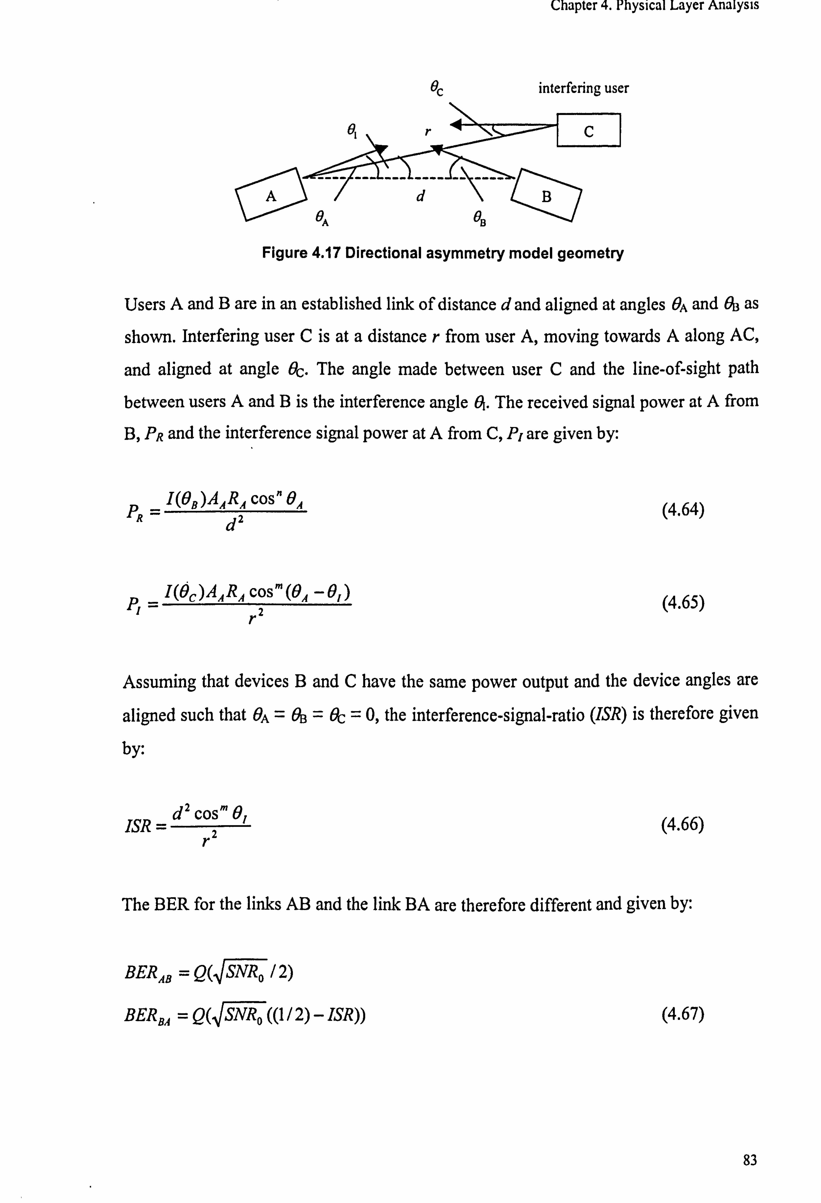
Chapter 4. Physical Layer Analysis
interfering user
C
Figure 4.17 Directional asymmetry model geometry
Users A and B are in an established link of distance d and aligned at angles BA and 6a as
shown. Interfering user C is at a distance r from user A, moving towards A along AC,
and aligned at angle Oc. The angle made between user C and the line-of-sight path
between users A and B is the interference angle 6i. The received signal power at A from
B, PR and the interference signal power at A from C, PI are given by:
p= I (9B )AARA cos" 9A
. da
I(Oc)AARA cos'" (6A -01) Pt =r2
(4.64)
(4.65)
Assuming that devices B and C have the same power output and the device angles are
aligned such that OA = 9B = Oc = 0, the interference-signal-ratio (ISR) is therefore given
by:
ISR = d2 COS m 9,
r2 (4.66)
The BER for the links AB and the link BA are therefore different and given by:
BER,, B = Q( SNRo l 2)
BERB,, = Q( SNRo ((1 / 2) - ISR)) (4.67)
83

Chapter 4. Physical Layer Analysis
0
10z
1o'
ce ui ý ýo"
lo'
10-10
024
--- link AB - link BA
68 10 12 14 16 18 20 Interferer approach distance r (m)
180
270
Figure 4.18 Directional BER asymmetry Figure 4.19 Interferer loci for constant BER versus interferer approach distance values with narrow angle transceivers
Figure 4.20 shows the BER of link AB and link BA versus the approach distance of interferer C with the link AB distance d set to lm. SNRo is the SNR from ambient light
only and is set to give a BER without interference of 10"8 (dotted line). It can be seen that the BER of link BA (solid line) begins to significantly degrade at an interferer
distance of 3m. Figure 4.21 shows the position loci of the interferer (angle 6i and distance r, Figure 4.19) to achieve BER values in the link AB of 10"5,10"6 and 10'7
using narrow angle transceivers (m = 20). This shows that if the interferer approaches from an angle greater than 30°, the approach distance can be less than 2 meters before
the BER is significantly degraded.
4.4.2 Spatial Asymmetry from Moveable Link with Fixed Interferer
In addition to directional asymmetry, spatial asymmetry can also occur in a link where
the BER varies with the spatial orientation of a receiver in relation to a fixed interferer.
This scenario can arise where two independent IR links are operating in close proximity. In the example situation, users A and C are in an established link and interfered with by
user B transmitting to unseen user D. User C is movable with respect to A, but
interfering user B is fixed and transmitting parallel to A with a separation distance d.
This is shown in Figure 4.22.
84

Chapter 4. Physical Layer Analysis
Figure 4.20 Geometry of spatial asymmetry scenario
The received power at device C from A and at C from B are given by:
(C, A) PA Ac (n + 1) COS" OA
P, =z 2m-,
(C, B) PB Ac (n + 1) COS" 9B COS' OC
P, -2 2)cr2
(4.68)
If we assume that all devices have identical transmitter and receiver characteristics, the
interference-to-signal ratio is then given by:
ISR = COS"BgCOS' Ocr, 2
COS" 0Ar22
Using trigonometry it can be established that:
r2 = d2 +r12 -2dr, cos(BA +ir/2)
ec =sin-' dsin(9,, +z/2)
L rz
(4.69)
(4.70)
(4.71)
85

( hnhtrr, 4. Physical I . aycr Analysis
H� _. U ,+H, . (4.72)
In this case the SNR (without interference) will also vary with the geometry of the link
AC. The SNR, can therefore he given by:
SNR = SNR, COS d1 (4.73) jl
where SNR� is the SNR to achieve a LOS BER of 10.8 with HA 0 and a' = lm. Figure
4.23 shows the polar plot of the loci of user C in relation to A (angle BA and distance r1)
to provide a BlR better than or equal to I0-ß (shaded areas) (Barker and Boucouvalas,
2002a, Barker and Boucouvalas, 20()2b) with varying separation c! of devices A and B
and with narrow and wide angle transceivers. This demonstrates how the separation
distance between two independent IR wireless links affects the spatial BER and
throughput of the links. It can he seen that there is a significant spatial asymmetry effect
using wide angle transceivers. For narrow angle transceivers, the effect only becomes
significant when the separation distance d is less than 0.4 meters. This therefore shows
that two independent links adhering to the minimum IrDA specification can be as close
as 0.4 in apart without mutual interference.
86

Chapter 4. Physical I aver , Analvsis
90 1 120 60 ý 0e
-+- .ý. O6
150ý ,..... \30 ý.
\-ýy"ý:
,`_... ..
v, 0'.
210ý '330
. _- ."' 240'...
.,. ._- 300
770
wide angle transceivers, d 0.8 in
'Nl
120 60
" 150, .\... ... 30
., t" 04
"
02-. y.. ..
180
: 10ý 170
..
740 100
; 711
narrow angle transceivers, d= 0.8 in
1)1 1 ý111 , 120 s0 170 0 0eý 08
150, // 311 06
150/ 30 0.4 ý
)
,`ý
'
2
-f 180 ~
-r r- F- ,0 180
\ ý\'
'\ /
i \ ýý-
21 0
\
\`j/ý
_ '\ 330
\\
- i1ýý
_
\\
X330
ý"/ ýJ
740.... 300 240 3011
270 770
wide ang le transceivers, d=0.4 m narrow angle transceivers, d=0.4 m
90 1 90 1 120 60 120 _---- 60
0.8 0.8
15ý 06y r'\
30 06 _ 30
0.4 "
02 ý
180, 0 180ý I 1i ý/
r/I i\ I l. ý- I
ý \
710C. '\ /330 ý_
/330
. ;' -" 2 . .v 40 300 '. 10 , 700
770 L711
wide ang le transceivers, d=0.2 m narrow angle transceivers, d=0.2 in
Figure 4.21 Spatial asymmetry for user C loci and AB separation distance d to provide BER < 10-8
87

Chapter 4. Physical Layer Analysis
4.5 Chapter Summary
In this chapter we have examined the physical layer characteristics of an IR wireless data link in order to establish expressions for the bit-error-rate (BER) and packet error
probabilities for specific data rates, modulation and encoding schemes. Expressions for
BER can be linked to the throughput analysis (Chapter 6) to provided throughput
performance in relation to physical layer characteristics. Expressions for the transmitted
optical power in terms of transmitter characteristics and modulation scheme are derived
and expressions for the received optical power are derived in terms of detector
characteristics and system geometry. Noise sources are examined to determine the noise
power from ambient background light induced shot noise. From these, expressions for
the SNR and hence BER of an IR link were derived. It is shown that there is a sharp cut-
off distance for link quality and that the receiver bandwidth for the required data rate is
a significant factor in performance. Third user interference is examined with resulting directional and spatial asymmetry effects. These indicate the minimum separation distance for independent links. The following chapter examines existing studies of data
link and media access protocols with the aim of choosing suitable methods for the
application to performance analyses of the IrLAP and AIr MAC protocols.
88
5. MODELLING OF COMMUNICATIONS
PROTOCOLS
This chapter examines methods that have been used in modelling general
communications protocols that are of relevance to the current study. In particular it
looks at analytical modelling of data link protocols and multiple access protocols.
5.1 Modelling HDLC Based Data Link Protocols
Data link protocols are primarily concerned with frame error detection and correction
and flow control regulation. Therefore in performance modelling of data link protocols
we are looking at the dependence of the end-to-end throughput on frame-error-
probability (simply related to the bit-error-rate) and the interaction with link parameter
settings and characteristics. Throughput is determined by calculating the proportion of
time spent successfully transmitting data to the total active time. This can be determined
in a number of ways depending on nature of the system being investigated (e. g.
balanced or unbalanced, full or half-duplex, saturated or unsaturated) and on other
assumptions of system behaviour.
5.1.1 The Virtual Transmission Time Method
Bux & Kummerle (1980) presented a method for determining the saturation throughput
of balanced full-duplex HDLC using the concept of the `virtual transmission time'
(VTT) for a data frame. This is defined as the time from the start of frame transmission
at the transmitter to the completion of successful frame reception (including possible
frame re-transmissions) at the receiver. The VTT for the last frame in a transmission
window also includes the time for the acknowledgement from the receiving station
before transmission can resume. The maximum frame throughput is then the reciprocal
of the average frame VTT.
89

Chapter S. Modelling of Communications Protocols
The model assumes a saturation data condition where data packets are continuously
available for transmission. It is also assumed that data traffic is passed in one direction
only and that S-frame acknowledgements are small enough to be considered error free.
The VTT for a particular frame is dependent on the window size (w) seen by the frame,
defined as the number of frames remaining to be transmitted before transmission must
stop due to M- 1 unacknowledged frames where M is the modulus of the transmission
sequence count (8 for standard HDLC, 128 for extended HDLC). The average virtual transmission time t, is then given by:
M-2
tv = FO(w)tv(w) (5.1) w=o
where O(w) is the probability of the frame having window width w, and tv(w) is the
window width dependent virtual transmission time.
The window width process for HDLC is modelled as the finite state machine shown in
Figure 5.1 where w is the variable window width and p is the probability of frame error. This is related to the link bit-error-rate pe by:
p=1-(1-pý)ý+r (5.2)
where 1 is the frame data size (bits) and 1' is the frame overhead size (bits). Taking a
maximum transmission window size of M-1 frames, the window width w is the
number of frames remaining to be transmitted following a transmission and thus has
values 0 to M- 2. Following a successful transmission the window size is reduced by 1.
However following a transmission failure (frame in error) the frame and following
frames in the transmission window will be re-transmitted from the start of the next transmission window. Thus the window width returns to the maximum M-2. This is
illustrated in the finite state machine diagram in Figure 5.1.
90

Chapter 5. Modelling of Communications Protocols
M-2 M--3
aºýº, I
Figure 5.1 HDLC window width process finite state diagram
lp
P
Using Markov analysis it can be shown that the probability «(w) of a frame seeing a
window width w is given by:
O(W) = PO - p) M-z-W
1- (1- p) M-l we {0,1, """, M-2} (5.3)
Calculation of the window width dependent VTT tv(w) depends on whether the
acknowledgement delay (tack) is greater than the window transmission time (where N is
the maximum window size and t1 is the I-frame transmission time) or not. This takes
into account possible propagation delays with long distance links (e. g. satellite). The
expressions for tv(w) are given by:
2
ty (w) = E[To (w)] + pE[T, (w)] +1pP T2
2
t, (w) = tj + pE[T ]+ T2 1-p
tack > Nt,
tack <_ Nt,
(5.4)
(5.5)
where To(w) is the time for the initial frame transmission, Ta(w) is time for the first re-
transmission (E[T! (w)] and E[To(w)] are the average or expected values) and T2 is the
time for subsequent re-transmissions. The value for T2 is independent of w because for
subsequent re-transmissions the frame considered will be the first in the re-transmission
window. These elements are expressed in terms of conditional time components and the
probabilities of the conditions occurring. The use of the virtual transmission time
provides a mechanism for determining throughput in relation to all operational
91

Chapter 5. Modelling of Communications Protocols
parameters (bit-error-rate, data packet length, frame overhead, window size, data rate,
propagation delay) and provides a clear explanation of the individual processes that
effect the performance (Schwartz, 1987). The model analyses full-duplex balanced
HDLC procedures but the method can be applied to all HDLC procedures with suitable
modifications.
The model by Bux was modified by Burakowski (1986) to model HDLC-ABM with dependent error channels in which the probability of a bit error is not assumed to be
independent but is dependent on the preceding bit success. This is assumed to be a more
realistic evaluation of bit-errors for real communications channels. The bit transmission
process is modelled as a Markov process. This results in a modification to the window
width probability distribution given in equation 5.3
ý(w) = p(E I C)[p(C I C)] M-2-w
1-[p(C I CAM-1 (5.6)
where p(E I C) is the probability of a bit error given a preceding correct bit and p(C I C)
is the probability of a correct bit given a preceding correct bit. The window width dependent VTT tv(w) formulae are also modified to include the above probability and
p(E), p(C) the probability of a independent error bit and correct bit respectively. This
analysis may be suitable for wired data links with low error rates or noise-burst error
conditions, but may not be suitable to IR wireless links.
5.1.2 Queuing Analysis Method
Queuing analysis is a common method for performance evaluation of communications
networks (Chan, 2000) where data packet service queues are a major bottleneck in the
network performance. Labetoulle and Pujolle (1981) determine the maximum
throughput for bi-directional error-free saturated HDLC-ARM links with non-uniform
packet sizes using queuing analysis. The model uses a system of N parallel servers
corresponding to the maximum window size. Packets arrive at service rate , ul and each
server has mean service time S. The model is an M/G/N/N queue with loss and the
throughput T is therefore given by:
92

Chapter 5. Modelling of Communications Protocols
pN
T=, u, 1- N! - -N �n
\1 ý ý n!
where p=p, "S
(5.7)
Such an analysis may be beneficial for land based or satellite HDLC links where the bit-
error-rate is very low but not suitable for wireless links with potentially high error rates.
5.1.3 Probabilistic Automaton
Masunaga (1978) developed a throughput expression for NRM half-duplex HDLC from
a probabilistic automaton (finite state machine). The point-to-point throughput was derived by reducing a four-state automaton of the two-way data transfer procedure between a primary (P) and secondary (S) station to a two state goal process. The
principal assumption made in this analysis is that either all frames in the window are
transmitted correctly or one or more frames including the final frame are in error and
the entire window re-transmitted. The four state finite state diagram is given in Figure
5.2.
The process flow is as follows.
So -- S1: P transmits window to S, P-bit frame not lost, probability Poi, time Tol
So -4 S2: P transmits window to S, P-bit frame lost, probability P02, time T02
S2 - S2: P re-transmits window to S, P-bit frame lost, probability P22, time T22
S2 -ý S 1: P re-transmits window to S, P-bit frame lost, probability P21, time T21
Si --ý So: S transmits window to P, F-bit frame lost, probability Plo, time T10
S1 -ý S3: S transmits window to P, F-bit frame not lost, probability P13, time T13
93

Chapter 5. Modelling of Communications Protocols
Pio, T1o Event 4
Po>>Toi Event 1
P22, T22 Event 2
a) Four state HDLC process 1, Tc
b) Two state goal process
Figure 5.2 HDLC half-duplex NRM finite state process and goal process
In reducing the four state machine to a two state machine from state So to S3 with time TC and probability of 1, the time TC (the average time to transmit a frame window from
P to S and S to P) is given by:
TC=T13+°T10+ 1+° P°1T°1ý'P02T°2ý"ý'°2T°1-! "P° 22T22
13 P3 P21 (5.8)
The time T11 and probability P1 (from state i to state j) are calculated from the HDLC
operational parameters and line bit-error-rate. The focus of the model is the impact of the time-out period when the P or F bit is lost. The assumption that the entire window is
either accepted or rejected may be acceptable for a small window size but not as the
window size becomes larger. It will certainly not be acceptable for the 127 frame
window size used with 16 Mbits/s VFIR.
From the above studies it can be seen that the analysis by Bux although based on balanced full-duplex HDLC procedures provides a very accurate analytical model with
minimal simplification assumptions for saturation throughput which may be applied to
94

Chapter 5. Modelling of Communications Protocols
the unbalanced half-duplex HDLC based IrLAP protocol. Other studies have
unacceptable assumptions or approximations (e. g. a low bit-error rate) for the analysis IR wireless links.
5.1.4 Simulation Studies of HDLC
A simulation study of HDLC links was presented by Georges and Wybaux (1981). The
study examined both saturated and non-saturated balanced HDLC links. For both cases
the data packet lengths are random with an independent three phase distribution. This is
intended to simulate random network data traffic consisting of 1) short network control
packets, 2) maximum length data packets, and 3) varying length data packets less than
the maximum. In the saturated condition, the input queue has just one place which is
occupied by a waiting data packet. This is immediately replaced by another when the
packet is transmitted. In the non-saturated case, data packets arrive at the input queue
according to a Poisson process with specified Mean Interarrival Time parameter (1 / 1v).
As the input queue in the saturated case is unbounded, 1/A. should remain greater than
the mean packet transfer time determined from the saturated case. The generation of
packet errors is also modelled on a Poisson process where the probability Pr of one or
more errors in frame of data length 1 is given by:
P, =1- er-eER (5.9)
Results of the saturation case help decisions on the transmission window size parameter
and acknowledgement timer duration parameter.
A simulation model of balanced HDLC using a Petri Net description and PROTOB
simulation environment was given by Marsan and Barbetta (Marsan et at., 1989). Petri
Nets are a formal description of dynamic systems that can be used for the specification
of communications protocols. The PROTOB simulation environment is based on a class
of Petri Net called Prot-nets that allows an object oriented development of a discrete
event simulation model with a graphical and textual environment.
95

Chapter 5. Modelling of Communications Protocols
Larue and Frost (1990) presented a technique for extrapolating the performance of HDLC links. The basis of their technique was to take the results from a single
simulation run for the HDLC protocol with a single error rate parameter and extrapolate
results for a range of error rates. This was aimed at reducing the computational load for
a simulation study at a time when computing processor speed was still limited. The
technique used involves the weighting of packet end-to-end delay values by the
probability that they would be observed under different operating conditions. This is a form of the ̀ importance sampling' technique.
Such studies are useful in highlighting the important issues in the simulation of data link
protocols that can be of benefit in the design of a simulation model for the IrDA 1. x
protocol (see Appendix A).
5.2 Modelling CSMAICA Medium Access Protocols
With multiple access schemes for a shared medium we are primarily interested in the
efficiency of network utilisation and end-to-end packet delays where collisions on the
medium force frame retransmissions.
5.2.1 Performance Models of CSMAICA
An analysis (Brewster and Glass, 1987) and simulation (Glass et al., 1988) of non-
persistent CSMA/CA was first presented by Glass and Brewster. The analysis examined both slotted and non-slotted CSMA/CA with Poisson distributed traffic load. The
throughput for the non-slotted case was given as:
e-aG S [1/G+3a+(1+a)e-aG +a(1-e-aG){3+(1/aG)-e-aG l(1-e-aG)}]
(5.10)
where as with the CSMA/CD analysis, G is the channel load and a is the normalised
propagation time.
96

Chapter 5. Modelling of Communications Protocols
The simulation model was developed using the SLAM II (Simulation Language for Alternative Modelling) language.
Further analyses of CSMA/CA have largely concentrated on the IEEE 802.11 MAC
protocol. As described in chapter 1, the IEEE 802.11 is a standard for wireless local area networks (W-LANs) using a common CSMA/CA based MAC protocol for a number of
physical layer options.
A major study of the performance of the IEEE 802.11 protocol has been produced by
Chhaya and Gupta (Chhaya and Gupta, 1997). This examined both the `basic' access
and RTS/CTS methods with non-saturated load using a mathematical analytical model
verified with simulations using OPNET. They also examined the effects of non uniform frame sizes and spatial analysis. In the analysis for the `basic' access method the
throughput S(i, j) from station i to j is given by:
SýI, J) = Ps ýl, l)( Gý^ 1)
+ ý1- e'ýcº, ýý )ý Gým, n) ss v m, n
(5.1 1)
where ps(i, j) is the probability of a successful transmission from station i to j. G(i, j) is
the offered load from i to j and G is the total load. The set (m, n) denotes all other
station pairs excluding (i, j). Ts is the average length the `renewal period' following a
successful transmission. This is the length of time between the medium being detected
free and is given by:
TS =1/G+DIFS+1 +/3+lack (5.12)
where 1 is the frame transmission time and 8 is the propagation delay.
Crow (Crow et al., 1996) produced a bespoke simulation model of the 802.11 MAC
protocol. The model investigated the performance of both the Distributed Co-ordination
Function (DCF) used for ad-hoc network configurations and the Point Co-ordination
97

Chapter 5. Modelling of Communications Protocols
Function (PCF) used for an infrastructured network configuration. With the latter there
is a central co-ordinating station that polls the other stations in sequence.
Bianchi (Bianchi, 1998; Bianchi, 2000) produced a mathematical model for the
saturated throughput of the 802.11 MAC DCF protocol using both the `basic' and RTS/CTS access methods. The analysis uses a Markov model of the exponential back-
off collision avoidance process.
The derived throughput is given by:
S= PsP, E[P] (1-Pn, )a +Pt, PSTs +P, r(1-Ps)Tc
(5.13)
where Ptr is the probability of at least one transmission in a particular time slot, given by:
r =I- t (1- z) (5.14)
where r is the probability of transmitting in a chosen time slot and n is the number of
stations in the network. PS is the probability that a transmission is successful and is
given by:
P= nz(1-z)"-ý s P, (s. is)
The component E[P] represents the expected transmission time for the packet size and
o' is the collision avoidance slot duration. The periods Ts and Tc are the time sensed on
the medium for a successful transmission and when a collision occurs respectively. These are illustrated in figure 5.3.
98

Chapter 5. Modelling of Communications Protocols
Source
Destination
Other
I Hdr (H) Payload (P)
Hdr (H) Payload (P)
Tc
TS
I SIFS ACK
DIFS I
a) Basic Access
Source
Destination
Other
ý RTS
ý
RTS
I SIFS
Tc
( SIFS ACK ICTS
DIFS
I S(FS
B) RTS/CTS Access
Figure 5.3 Basic and RTS/CTS access times for 802.11 DCF
DIFS I
These depend on the access method used. For the basic and RTS/CTS methods, the
successful transmission media time TS and collision transmission media time Tc
respectively are:
Ts`ý =H+E[P]+SIFS+ß+ACK+DIFS+ß
Tcb' = H+E[P']+DIFS+, 8
Ts1s = RTS+SIFS+Q+CTS+SIFS+/3+H
+E[P]+SIFS+ß+ACK+DIFS+, Q
Tb c' = RTS + DIFS + ýl3
(5.16)
(5.17)
where each element is a time component. H is the packet header duration and 8 as before is the propagation delay. The value E[P*J is the average length of the longest
packet in a collision. If a fixed data packet size is used then we simply have E[P] = E[PýJ = P.
TS
DIFS
I Hdr (N) Payload (P)
99

Chapter 5. Modelling of Communications Protocols
The probability r of transmitting in a particular time slot is provided by the Marköv
model analysis of the exponential back-off process and gives:
T= 2(1- 2p)
(1-2p)(W + 1) + pW(1-(2p)') (5.18)
where W is the initial contention window size CWmin and m is the maximum
exponential back-off stage such that CWmax = 2mCWmin. The value p is the probability
of collision and is given by:
p =1- (1- Z)"-' (5.19)
This results in a non-linear system in p and rwhich must be solved numerically.
This model is based on the exponential contention window back-off process used in the 802.11 DCF protocol but can equally be applied to the linear contention window back-
off process of the AIr MAC protocol with suitable modifications.
5.3 Chapter Summary
This chapter has provided a review from published literature of methods used for
performance modelling of communications protocols that are relevant to the present
study. This involves data link layer protocols and shared media access protocols using both mathematical analytical and simulation methods. The methods used for maximum throughput in saturated data conditions and for non-persistent data with variable packet
sizes is also examined. The following chapter presents an analytical model of the IrDA
IrLAP protocol with performance results and optimisation analysis. The model is based
on the HDLC performance model of Bux, described in this chapter.
100

6. IrDA 1. x PROTOCOL PERFORMANCE
MODELLING This chapter presents an analytical model of the IrDA 1. x IrLAP data link protocol information transfer process. The model provides saturation throughput in relation to the
link BER and other protocol parameter settings. Graphical results are presented for
theoretical maximum link throughput and in relation to varying BER and link parameter
values. This leads to optimum values for the data packet size and transmission window
size.
6.1 IrDA IrLAP Analytical Model
The model presented here is an evolution of the model given by Bux and Kummerle
(1980) which analysed balanced full-duplex circuit HDLC procedures, to the analysis of
the un-balanced half-duplex HDLC based IrLAP protocol. The basis of the model is to
calculate the average ̀virtual transmission time' (VTT) for a frame being transmitted in
an IrLAP link. The VTT is the total time taken for the reliable end-to-end transmission
of an I-frame between peer IrLAP layers. The VTT of a specific frame begins at the
start of the frame transmission and ends with the successful reception of the frame (or
frame re-transmission) in-sequence and without error at the receiving station. The VTT
for the first frame in a transmission window must also include the time for the
acknowledgement reply (including link turnaround delays) from the receiving station for the previous window.
The VTT is calculated using the probability of packet error based on a specified BER
and on the re-transmission times required for a particular packet position within the
transmission window. The probability of the packet being in a particular window slot is
determined by a Markov model of the window width process. The average saturation
throughput is therefore given by the reciprocal of the average virtual transmission time
multiplied by the packet data size. The model thus provides the theoretical maximum
IrLAP link throughput in terms of the link BER and link parameter settings of link data
rate, data packet length, maximum window size, maximum turn-around time (window
transmission time) and minimum turn-around delay.
101

Chapter 6. IrDA Ix Protocol Performance Modelling
6.1.1 Model Assumptions and Parameters
The model assumes a primary and secondary station pair operating in the data exchange
phase of the IrLAP procedure. All user data packets (i. e. I-frames) are transmitted from
the primary to the secondary only. The link is assumed to be saturated, i. e. there is data
continually waiting transmission at the primary (thus the P-timer is not of relevance).
The secondary responds with RR (Receive Ready) S-frames only. It is assumed that an S-frame, whether from the primary or secondary, is small enough to be considered error free. The action of the F-timer is incorporated when the primary forces a reply from the
secondary if there is corruption of aP bit frame. As link distances are very small, the
propagation delay is negligible.
The following input parameters are used in the analysis:
Parameter Description Unit C Link data baud rate bits /sec Pb n Link bit error rate - ldata I-frame data packet length bits loh S-frame length / I-frame overhead bits tra Minimum turn-around time sec Tmax Maximum turn-around time sec W�, ax Maximum window size frames
Table 6.1 IrDA analytical model Input parameters
The S-frame transmission time is and I-frame transmission times tl are calculated by:
ts -1-" C
t_1 dnla + loh
rc
(6.1)
(6.2)
The acknowledgement time tack is the time following the completion of transmission from the primary, for an acknowledgement S-frame to be returned from the secondary
and the primary to resume transmission. This therefore requires a turn-around delay at the secondary, the transmission time of the S-frame and a turn-around delay at the
primary.
102

Chapter 6. IrDA 1. x Protocol Performance Modelling
tack = 2tla + tS (6.3)
The frame error probability p is the probability that there is at least one bit in an I-frame
in error, and is therefore related to the link bit error rate pe by:
P_ 1_(1 - PC )I oA+ldam (6.4)
The variable window width w is defined as the number of remaining frames (from the
start of the current frame) that can be sent before transmission control is passed. With
IrDA, the maximum window width is determined by the `maximum window size'
parameter, here denoted Wm, negotiated during the link establishment, and the
maximum turn-around time combined with the data rate and packet data size which may limit the number of frames that can be sent to below Wmax. We therefore use a value N
to indicate the number of frames that can be sent before transmission is passed to the
other station.
T" - N= min W,,.,, floor
,
where min is `the lesser of, and floor is the rounded down integer.
(6.5)
The F-timer timeout period tFvur could be set to the maximum turn-around time T, �,,,, however this could cause an unnecessary delay when the full window is returned well
within this period. Therefore we can set the F-timer period to the maximum time
(assuming the same packet size) that would be required to return an F-bit packet from
the Secondary. This is therefore:
t Fout -
Nil + 2tta (6.6)
103

Chapter 6. IrDA 1. x Protocol Performance Modelling
6.1.2 Calculation of the Virtual Transmission Time
The average virtual transmission time is determined by summing the frame virtual
transmission times for all values of w, multiplied by the probability of the frame having
each value of w. This is therefore given by:
N
tv =E o(w)tv(w) (6.7) w=1
where tv(w) is the virtual transmission time for a frame seeing a window width w, and O(w) is the probability that the window width has a specific value of w. The average data throughput D (bits/s) is then given by:
1 data
tv
6.1.2.1 Window Width Probability
(6.8)
Each time a frame is transmitted error free (with probability 1- p), the window width
reduces by I (Figure 6.1a). When it reaches 1, the window width returns to its
maximum value of N. However if a frame is in error (with probability p) then it and all the following frames in the window will need to be re-transmitted. The next transmission window will therefore begin with re-transmission of the errored frame
(Figure 6.1b). Therefore following the successful transmission of the errored frame the
window width is N-1. This is demonstrated in Figure 6.1 where sub-Figure (a)
represents an error free situation and sub-Figure (b) has frame 130 (I-frame, Ns = 3, Nr
= 0) in error.
104

Chapter 6. IrDA I. x Protocol Performance Modelling
(1-p) (1-P) (l-P) (I-p) 0-P) (1-p)
w=7 w=6 w=S w=4 w=3 w=2 w=1
(a)
O-p) 0 -P) O-p)
w=7 w=6 w=5 w=4 w=3 w=2 w=1
(b)
(ý-p)
S7F
S3F
w=7
. "'o. I
Figure 6.1 Window width states for N=7 (a) error free, (b) frame 130 in error
w=7
The overall process can be considered as a Markov chain with N states representing the
widow width values. This can be presented as the state transition diagram shown in
Figure 6.2 where the solid line represents an error free frame transmission (with
probability I -p) and the dashed line represents frame error transmission (with
probabilityp).
Ip
------ p
---------------------
(P)
-- e
Figure 6.2 Markov process diagram for IrLAP window width process
The value for O(w) in (6.7) can then be determined by calculating the `limiting (i. e.
steady-state) probability distribution' for the window width state set in Figure 6.2. The
state transition diagram can be represented by the state transition matrix R, where the
probability of going from a state i to a state j is given by the element rj.
105

Chapter 6. IrDA I. x Protocol Performance Modelling
R
(N-1) (N-2) ... (w) ... (1) (N)
p 1-p 00000
p0 1-p 0000
p00 I- P000 (6.9) p000 1-p 00
p0000 1-p 0
p00000 1-p
1000000
(N-1) (N-2)
(w)
(1) (N)
If we define the limiting probability distribution vector Q such that
Q=[O(N) ... O(W) ... 0(1)l (6.10)
using matrix multiplication we can determine Q by using the Markov equality (see
Appendix B):
Q=R .Q (6.11)
This gives the set of simultaneous equations
N-I
pyO(w)+O(N) _ O(N-1) W-1
(1- P)O(i) = O(i -1) i r. (2, N -1) (1- P)0(1) = O(N)
and N
F, o(w) =1 »sl
therefore equation (6.12) becomes
p(1- O(N)) + O(N) = O(N -1)
which can be re-arranged as (1- p)O(N) +p= O(N -1)
(6.12)
(6.13)
(6.14)
(6.15)
(6.16)
(6.17)
106

Chapter 6. IrDA Lx Protocol Performance Modelling
we also get
O(N) = (1- p) N-'O(N -1)
combining the above we get
O(N-1)-1-(lp P)N
and since O(w)=(1-p)O(w+1) w=1,2"""N-1
this gives us
(6.18)
(6.19)
(6.20)
P(1- p)"-" w=1,2"""N-1 1-(1-p)N
O(w) = P(1- P)N-1 1-(1 P)N
w=N
(6.21)
This provides an expression for O(w) for equation (6.7) in terms of the packet error
probability p and maximum window width W.
6.1.2.2 Window Width Dependent Virtual Transmission Time
The window width dependent VTT t, (w) is calculated by the addition of the time to
transmit the initial frame and the time required for subsequent re-transmissions of the
frame multiplied by the probabilities that these re-transmissions are required.
CO
tº'(w) =To(w)+1: PnE[Tn(w)J
n=l
(6.22)
107

Chapter 6. IrDA l. x Protocol Performance Modelling
where To is the time to transmit the frame initially P� is the probability that the nth re-
transmission is required, and E[T� (w)] is the expectation value of the time required for
the nth re-transmission.
In calculating the virtual transmission time we need to examine a number of different
cases involving whether an error occurred, in what position in the window the error is
located, whether there are additional errors in the sequence and in what positions, and
whether the re-transmissions of frames are themselves in error.
A. Initial frame transmission time
The transmission time in this situation is simply the transmission time for the I-frame
unless the frame is the first frame of a window (i. e. w= N) in which case the primary
station must wait to receive an acknowledgement from the receiving station for the
previously transmitted window before continuing to transmit. This is shown in Figure
6.3.
To(4) ý
1 100 no 120 160P r -1
To(11q
\\ ýý
\ S7F
'I
I30 140 150
Iý 1 -ý r� E-ý
Is
tack
Figure 6.3 Case A transmission times
The initial frame transmission time To is therefore given by:
To (w) - ti w# N
tl + tQck w=N
Eý t�
-ý
1 170
E 11 '1
(6.23)
108

Chapter 6. IrDA 1. x Protocol Performance Modelling
B. Re-transmission of a frame in error
This case examines the situation where a frame transmitted needs to be re-transmitted because it has been in error. This case has the probability of a single error, i. e. p. The
time TI(w) denotes the time taken from the end of the initial errored frame transmission
to the end of the first frame re-transmission. We need to examine whether we have
additional errors following the initial error frame, and whether this includes the last
frame in the window.
B(i) Single error, not last in window This is illustrated in Figure 6.4. Here the frame is simply re-transmitted at the end of the
sequence and after the S-frame has been returned. The re-transmission time Tj(w)
includes the transmission time for any following frames in the window, the
acknowledgement time from the secondary and the frame re-transmission time.
I00 no 120 140 150
K (w-I)r1
160P
T, (4)
i 'ii
H3IT
I30 1
I( )p tack
Figure 6.4 Case B(i) re-transmission time
T, (w) = wtr + tack
F-ý !i
(6.24)
B(ii) Errors including last in window This is illustrated in Figure 6.5. In this case the P-bit is lost, therefore the secondary will
not know that it can now transmit. If the primary has not received a response when the
F-timer has expired aP bit will be sent with an RR S-frame. This situation has an
109

Chapter 6. IrDA 1. x Protocol Performance Modelling
additional probability ofp, i. e. the probability of a specific frame (the last) following the
first corrupted frame being in error. Note that additional frame errors within the window
not including the P-bit frame will not effect the throughput as all frames from the initial
errored frame within the window are retransmitted.
r 140 150 -[>9! 2
c
(w-J)ty E
T, (4)
SOP
ý T ýT
S3F
ý
130 1
E> 'Pout 's ',., k '1
Figure 6.5 Case B(ii) re-transmission time
T(w) =wtl+ ti Pout +ts+ tack (6.25)
B(iii) Single error being the last in the series This case is the same as case B(ii) above with w=1 except that there is only one error in the sequence, thus there is only the single error probability.
Therefore by combining equations (6.24) and (6.25), with the stated additional
probabilities the overall expectation value of Tj(w) and the probability Pl can be given
by:
P, =p
ELTi(x'), = wt, +p(tFout+tS)+tack w61
tl + tFout + tS + tack w=1
(6.26)
(6.27)
110

Chapter 6. IrDA 1. x Protocol Performance Modelling
C. Secondary re-transmissions due to subsequent frame errors
As the initial resent frame will be the first in the window, all N frames will be re-
transmitted. Therefore the re-transmitted frame will always be the first in the window. However as before if the last frame of the sequence is also in error, the P bit will not be
received so the recovery only begins when the F-timer expires. The probability of n
successive transmissions of the same frame being in error is p". Thus we have:
P"=p" 11>_2
and by using:
ýPn _
p2
n=2 ý1 pý
ý
gives: 2
j: 1',, E[Tn(w)]= P T2 n=2 (1- P)
(6.28)
(6.29)
(6.30)
where T2 is the time for each successive re-transmission of the frame and is now
independent of the window width w, given by:
Ntl +p (tFout + tS)+ tack Tz = tJ + tFout + tS + tack
N#1 N=1
(6.31)
The overall virtual transmission time for a specific value of w can therefore be
determined by using the expression in equation (6.22) and applying the derived
expressions for the expectations of the individual cases as shown above, combined with
the stated probabilities of each case arising.
2
tv (w) = To (w) + pE[T (w)]+ p TZ (1- p)
(6.32)
111

Chapter 6. IrDA I. x Protocol Performance Modelling
In summary the saturation condition throughput D (bits/s) is given by:
Throughput
D= ldata /tv
Average virtual transmission time N
L Y' , /, tV -
(w)tv(w)
w=1
Window width probability
p(1- p)"-"
O(w)
p(1- p)" 1-(_
O(w) =
w=1,2"""N-1
w=N
Window width dependent virtual
transmission time z
t(w) = To (w) + pE[T, (w)]+ p T2 0- P)
Packet error probability
p=1-(l-Pe)! °"+idw
Calculated window size
N= min W1118x, floor Tmex
tj
Initial frame transmission time
_ ti w #N
TO ýwý tl + t"k w=N
First re-transmission expectation time
-Ll\/JIa. a"a". _-I E[T. (w)l =
I Wt1 +P(tFou! +tS) + tack W36
1 t1 + tFour + tS + tack w=1
Second and above re-transmission time
Nt, + p(tFo,, r + ts )+ tack N# 1 T2 = tl + tFour + tS + tack N=1
S-frame and I-frame transmission times
is-1C tr_'data Cloh
Acknowledgement time
tack = 2tta + tS
F-timer duration
tFouf = Nt, + 2t1a
These expressions therefore provide the saturation throughput in relation to the data
rate, link BER and IrLAP parameter settings of data packet size, window size,
maximum turn-around time and minimum turn-around time (Barker and Boucouvalas,
1998a; Barker and Boucouvalas, 1998b; Barker and Boucouvalas, 1998c; Barker et al., 2000).
[I t [Four t rs t rack W= 1
112

Chapter 6. irDA Lx Protocol Performance Modelling
6.1.2.3 Bi-directional Data Flow Throughput
The model has so far assumed that the secondary returns error-free S-frame
acknowledgements only. However, if both the primary and secondary are transmitting
saturated data, the acknowledgement time seen at the primary would be extended to
cover the return of a full I-frame window from the secondary.
tack = Nt, + 2tta (6.33)
The throughput from the primary to the secondary will not concern errors in the
returned I-frames from the secondary unless the last frame in the window (with F-bit
set) is lost causing expiration of the F-timer. There is therefore an additional probability that the F-timer will expire (i. e. if either the last frame in the transmitted window or the
last frame in the returned window are in error). Following expiration of the F-timer an S-frame is transmitted to the secondary (assumed error free). The secondary will then
transmit the next window of I-frames (with re-transmissions if errors occurred) with the
F-bit on the final frame. There is therefore a probability of further F-timer expirations if
the last returned frame is again in error. Assuming the same frame error rate in both
directions, the window width dependent virtual transmission time tv(w) is now given by:
t(w) = To (w) + pE[T, (w)]+ P2 TZ +p (tFout + ts ) (1- P) 0- P)
6.1.2.4 F-timer Duration
(6.34)
If the P-bit frame or returned F-bit frame from the secondary is lost, the primary must
wait for the expiration of the F-timer before sending an S-frame to re-poll the
secondary. This delay can significantly affect the link throughput. The secondary station
will only return data frames if it immediately has data available to transmit. The F-timer
period may then be set to the maximum duration that may be required to return the F-bit
in a sequence of data frames. The F-timer duration has therefore been given as:
TF-timer =t ta
+ Nt / (6.35)
113

Chapter 6. IrDA l. x Protocol Performance Modelling
However this duration can still be excessive in respect to the acknowledgement time if
the secondary is not returning data but only returning an S-frame. Generally the primary cannot know if the secondary has data to transmit or not and thus must set the F-timer to
the duration as given. However there may be some applications where the secondary will only reply with S-frames (e. g. a printing application) in which case the F-timer may be set to cover this acknowledgement timer only:
TF-timer = tjQ +ts (6.36)
In practice an additional small delay may also be required for processing of the received F-bit frame or the timer `latched' until any frame reception and processing is complete.
6.1.3 Optimum Packet Length and Window Size
The throughput of a link for a particular BER is affected by the packet length and window size parameter settings such that optimum values can be determined to maximise the throughput. This is achieved by fording the value for which the first order derivative of the throughput with respect to the parameter is at zero, i. e.:
'data such that dDb (! data) _0 d1 data
and W,, such that dDb (W�aX)
=0 dW,,. X
(6.37)
(6.38)
It is possible to find the exact analytical first order derivative of the throughput with respect to 'data and Wm , but this would be mathematically complex. By using suitable approximations (Vitsas and Boucouvalas, 2000; Vitsas and Boucouvalas, 2001a; Vitsas
and Boucouvalas, 2001c) expressions for the optimum window and packet size have been obtained.
114
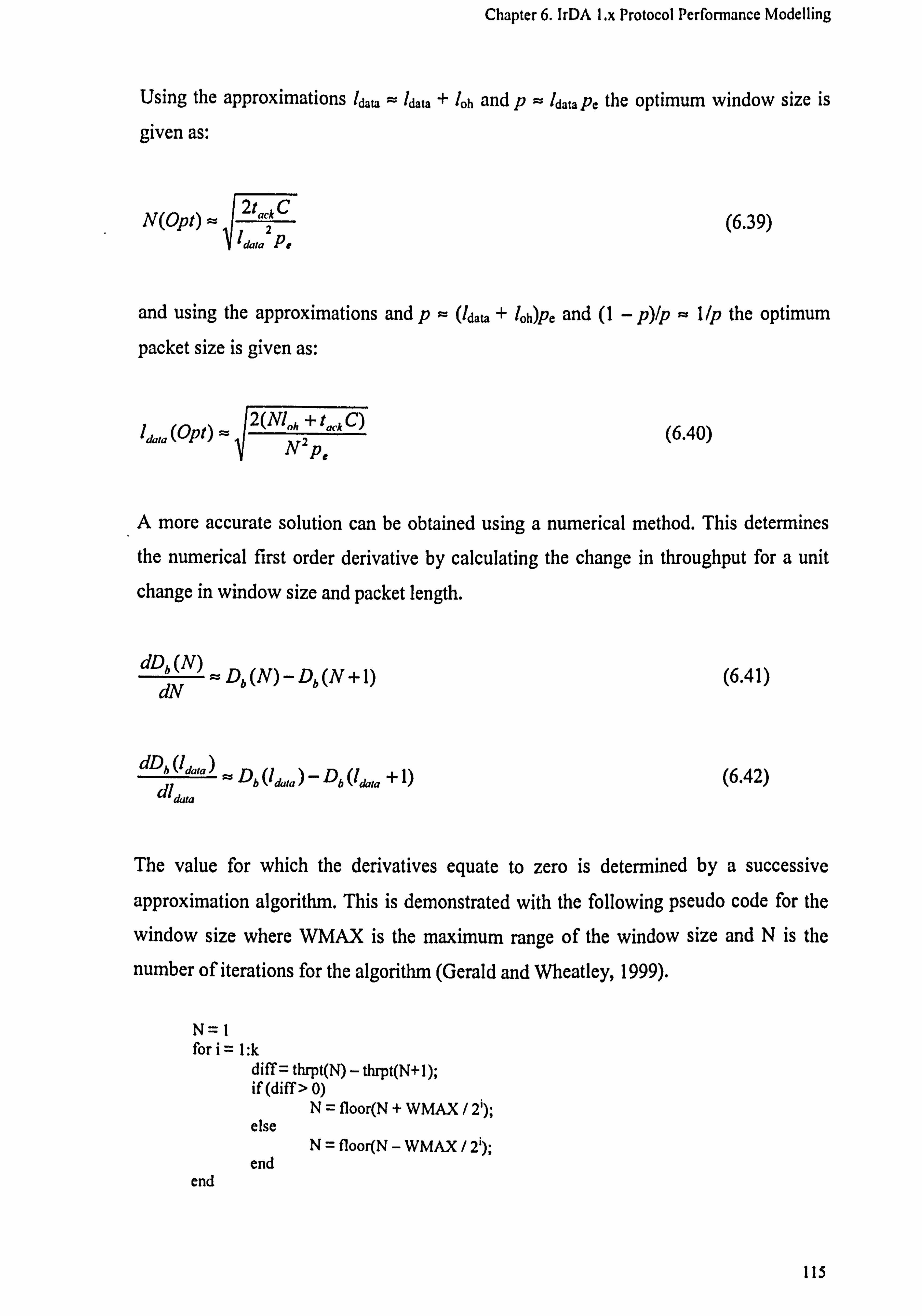
Chapter 6. IrDA Lx Protocol Performance Modelling
Using the approximations Idata ' /data + loh and p= Idata pe the optimum window size is
given as:
N(Opt) ý 2tack C
Idata ZPe (6.39)
and using the approximations and p- (Idaca + /oh)pe and (1 - p)Ip - 1/p the optimum
packet size is given as:
2(Nl,, h + tack C) ldala (OP') - NZP e
(6.40)
A more accurate solution can be obtained using a numerical method. This determines
the numerical first order derivative by calculating the change in throughput for a unit
change in window size and packet length.
dDb (N) --b� ýý De(N)-Db(N+1) (6.41)
dN
dDb Udala )
=Db Ydata )- Db Vdata + 1) dldata
(6.42)
The value for which the derivatives equate to zero is determined by a successive
approximation algorithm. This is demonstrated with the following pseudo code for the
window size where WMAX is the maximum range of the window size and N is the
number of iterations for the algorithm (Gerald and Wheatley, 1999).
N=1 fori= l: k
diff= thrpt(N) - thrpt(N+1); if (diff > 0)
N= floor(N + WMAX / 2');
end
else
end N= floor(N - WMAX / 2');
115

Chapter 6. IrDA I. x Protocol Performance Modelling
The larger the value of k, the higher the degree of accuracy. It can be seen from
equations (6.37) and ( 6.38) that the optimum window size is dependent on the packet
size and the optimum packet size dependent on the window size. It would therefore be
advantageous to obtain the simultaneous optimisation of the both the packet size and
window size (Boucouvalas and Vitsas, 2001).
This can be obtained by solving for the partial simultaneous differential equation.
aDh (N) _ aDb (rdata o aN al dýra
(6.43)
This produces the approximate results (Vitsas and Boucouvalas, 2001b)
oh
N(Opt)" a 2tackC
I dara iOPt) .= loti Pe
(6.44)
*= only optimum when both parameters are simultaneously optimised.
(6.45)
It can be seen that the optimum window size is dependent on the minimum turn-around
delay and the link data rate but is independent of the bit-error-rate. Conversely the
optimum packet size is dependent on the bit-error-rate but is independent of the data
rate and minimum turn-around delay. These results can also more accurately be
obtained as before with numerical optimisation.
116

Chapter 6. IrDA Lx Protocol Performance Modelling
6.1.4 Validation of IrLAP Analytical model
The graph in Figure 6.6 shows a comparison of results for a4 Mbits/s link from the
analytical model and the OPNET simulation described in appendix A The graph
demonstrates a good agreement between the two results. Table 6.2 shows comparison
numerical results from the analytical and simulation models for the 4 Mbits/s link with a
turn-around time of 0.1 ms and using a simulation time of 100 seconds. Differences are
principally due to the simulation time taken for the simulation run. For the simulations
for BER values of 10-9 and 2x 10'9, no errors occurred during the simulation time. For
the BER values of 4.8x10 and 10"3, all packets were in error during the simulation
time.
IrLAP Performance Analysis
0.9
0.4
0.3-
0.2-
oýýý 1011 105 107 10$ 105
Link BER
- analysis simulation: A min to time= 0.1 ms simulation: o min to time =I ms simulation: Q min to time = 10 ms
10,
data rate =4 Mbits/s max to time = 500 ms window size =7 frames packet size = 16384 bits
Figure 6.6 Simulation and analysis model results comparison for 4 Mbits/s IrDA link
117

Chapter 6. IrDA 1. x Protocol Performance Modelling
BER Throughput Efficiency (Analysis)
Throughput Efficiency (Simulation)
le-9 0.988608404 0.988652 2e-9 0.988527163 0.988652 4e-9 0.988364704 0.988324 9e-9 0.987958701 0.988201 1.8e-8 0.987228417 0.98689 3.8e-8 0.985607960 0.984433
7.8e-8 0.982376928 0.981647 1.6e-7 0.975794286 0.974602 3.3e-7 0.962320818 0.962724 6.9e-7 0.934543253 0.937165 1.4e-6 0.882623745 0.886866 2.9e-6 0.784270692 0.789996 6.1 e-6 0.616598022 0.621036 1.3e-5 0.385803960 0.383427 2.6e-5 0.186672727 0.190792
5.4e-5 0.062094262 0.062587 1.1e-4 0.015085827 0.014377 2.3e-4 0.001665257 0.001393 4.8e-4 2.632210195e-5 0 1 e-3 5.044571374e-9 0
Table 6.2 Numerical comparison of 4 Mbits/s IrDA 1. x simulation and analysis results
6.2 IrLAP Analysis Results
The following performance results are produced using the IrLAP throughput
expressions derived in the previous section. Numerical optimisation results are
presented for data packet size and transmission window size.
6.2.1 IrDA SIR 115.2 kbits/s Analysis
Figure 6.7a shows throughput efficiency versus data packet size for a 115.2 kbits/s link
with a BER of 10"9 and minimum turn-around times of 10,1 and 0.1 ms. This also uses
the maximum requested window size for IrDA SIR of 7 frames. It can be seen that the
throughput increases with packet size as the relative size of the overhead from the
frames and minimum turn-around time is reduced. The `jerky' nature of the analysis
plot at the higher packet sizes is due to the quantised reduction in the calculated window
size that can be transmitted within the maximum turn-around time of 500 ms. Note that
at the maximum specified packet size of 16384 bits (2 Kbytes) at 115.2 kbits/s, the
maximum window size that can be transmitted within 500 ms is only 3 frames. Figure
118

Chapter 6. IrDA I. x Protocol Performance Modelling
6.7b shows the performance for the same configuration but with a BER of 10"5. It can be
seen that the throughput initially rises, peaks (at around 103 bits for a turn-around time
of 0.1 ms) and then falls as the probability of packet error increases. This demonstrates
the requirement for optimisation of the data packet size to maximise throughput. It is
also seen that the optimum packet size is higher (although the maximum throughput is
lower) for a higher minimum turn-around time.
Figure 6.8a shows throughput efficiency versus requested window size for 115.2 kbits/s
with a BER of 10'9 and maximum data packet size of 16384 bits. This shows how the
throughput improves as the window size increases from I to the maximum of 3. Figure
6.8b shows the performance for the same configuration but with a BER of 10'5. For this
error rate the performance reduces as the window size increases. However the change in
throughput, particularly for a small turn-around time, is minor and only significantly
affected by a change in the packet size.
Figure 6.9 shows the optimum packet size for the 115.2 kbits/s link with the maximum
requested window size of 7 frames. The nature of the plots at low BER values is due to
the quantised reduction in the frames that can be transmitted within the 500 ms
maximum transmission time. The data packet size maximises at the maximum size that
can be send within 1 frame within the maximum transmission time of 500 ms,
calculated as 57551 bits. Note that this exceeds the maximum specification packet size
of 16384 bits. Figure 6.10 shows the optimum window size for the 115.2 kbits/s link
with a data packet size of 16384 bits. It can be seen that the optimum window size
changes from 2 frames to 1 frame but at a BER value that increases with the minimum
turn-around time.
Figure 6.11 shows the optimised data packet size for the 115.2 kbits/s link with
simultaneously optimised transmission window size. This shows an effective independence of the optimum packet size from minimum turn-around delay until the
reduction of the window size. Figure 6.12 shows the optimised window size for the 115.2 kbits/s link with simultaneously optimised data packet size. The window size increases with decreasing BER until the increasing packet size causes a reduction in the
119

Chapter 6. IrDA I. x Protocol Performance Modelling
window size that can be transmitted within the maximum transmission time of 500ms.
For the 10 ms minimum turn-around delay, the optimum window size increases beyond
the maximum 7 frames.
Figure 6.13 shows throughput efficiency versus BER using maximum, optimum and
simultaneous optimum packet sizes and window sizes. It can be seen that simultaneous
optimisation improves the performance over using maximum values. At a BER of 10-4 , the throughput efficiency improves by approximately 75% with optimisation. It can also be seen that the greater effect is from optimisation of the data packet size. At a BER of 10-4 , the throughput efficiency improvement from packet size optimisation alone is
approximately 65%. Figure 6.14 shows throughput against link distance using the
derived BER expression for 115.2 kbits/s with transmitter radiant intensity of 109
mW/Sr, receiver bandwidth of 250 KHz and link parameters from Tables 4.3. This
shows that optimisation provides a more gradual `fall off in throughput with link
distance than with maximum values which is quite abrupt. The `cut-off distance at this
data rate can be seen to increase by approximately 1 meter.
In summary, simultaneous optimum values are found for the data packet size and
transmission window size that maximise throughput for a given BER value and
minimum turn-around delay time. The effect of optimisation is to increase the
throughput for a given BER over fixed values. The dominant effect is that from
optimisation of the data packet size.
120

Chapter 6. IrDA Lx Protocol Performance Modelling
0.9
0.8
0.7 10.8
. 10. S
0.4
0.3
0.2 o. i
IrLAP Performance Analysis
min to time 10 me min to time 1 me
-- mintotime 0.1me
//
/ý
ý'ý
,/
,/ "/
'I , ii
/
I 16384 bits
100 101 i2 10° Packet Size (bits)
a) BER = 10"9
io'
0.9
0.8
ý 0.7
0.6
Q+s
0.5
0.4
0.3
0.2
0.1 . ...... I U
tOs 10°
data rate = 115.2 kbits/s window size =7 frames max to time = 500 ms overhead = 48 bits
0.98
0.96
0.94
0.92
0.9
102 103 104 105 Packet Slze (bits)
b) BER = 10's
Figure 6.7 Throughput versus packet size for 115.2 kbits/s IrDA SIR link
IrLAP Performance Analysis
ý----------------------------------- I
0.88F min to time " 10 ma min to time 1 ms
-- min to time 0.1 ma a. 88'
12345 Window Size (frms)
0.95F
0.9
0.85
0.8 u IR W
min to time 10 me min to time 1 me
-- min to time 0.1 me
V. /7
0. % I.. SýS : Sa
0.65
0.6-
0.55
7234 Window Siz" (hm")
a) BER = 10'9 b) BER = 10'5
data rate = 115.2 kbits/s packet size = 16384 bits max to time = 500 ms overhead = 48 bits
Figure 6.8 Throughput versus window size for 115.2 kbits/s IrDA SIR link
kLAP Performance Analysts
-- min to time in 10 me min tatime 1me
-- mintotime "0.1me , '% rýý.
ti
10'
litAP Pegormanc" Analysis
6 r
121

Chapter 6. IrDA l. x Protocol Performance Modelling
min to time 10 ma -- min to time 1 me -- mintotime -0.1me
n2 m ý
.ý
E_ ý1
I I iý '---'--
104 104 104 10 3 104 104 107,104 10 S 104 10 3 BER BER
data rate = 115.2 kbits/s window size =7 frames max to time = 500 ms overhead = 48 bits
data rate = 115.2 kbits/s packet size = 16384 bits max to time = 500 ms overhead = 48 bits
Figure 6.9 Optimum packet size versus link BER Figure 6.10 Optimum window size versus BER for 115.2 kbits/s
10
- min to time " 10 me min la time 1 me
-- min to time 0.1 ma
10ý 10ý 10' 10+ 10A 10-4 10' BER
data rate =115.2 kbits/s window size =optimum max to time = 500 ms overhead = 48 bits
for 115.2 kbitsls
n 10° 10,10,10
BER
min to time " 10 me min to time "1 me
-- mintatime 0.1me
10° 10, le
data rate =115.2 kbits/s packet size =optimum max to time = 500 ms overhead = 48 bits
Figure 6.11 Simultaneous optimum packet size Figure 6.12 Simultaneous optimum window size versus link BER for 115.2 kbits/s versus BER for 115.2 kbits/s
122

Chapter 6. IrDA l. x Protocol Performance Modelling
-. -,
0.9 0.8
0.7
0.6
w ý 0.5
0.4
0.3
0.2
0.1
oL-- 10'
\
\ ý
\
ý
.. 1 . "1 .1
108 i05
\
\
10, BER
103
data rate = 115.2 kbits/s min to time = 0.1 ms max to time = 500 ms overhead = 48 bits
Figure 6.13 Throughput efficiency versus link BER for 115.2 kbits/s link with maximum and optimum packet and window sizes
0.9
0.8
0.7 ý 0.6 1.0.5
0.4
0.3
0.2
0.1
-I= 16384, W=7 -I= 16384, W= Wopt --" I=Iopt, W=7 -I= Iopt(sim), W= Wopt(sim)
0.5 1 1.5 2 2.5 3 distance (m)
3.5
10 Y
10l
4.5
data rate = 115.2 kbits/s min to time = 0.1 ms max to time = 500 ms overhead = 48 bits transmitter power = 109 mW/Sr bandwidth = 250 KHa
Figure 6.14 Throughput efficiency versus link distance for 115.2 kbits/s 3/16 RZI link with maximum and optimum packet and window sizes
- 1=16384, W=7 - 1=16384, W=Wopt
--- I=Iopt, W=7
- I=Iopt(sim), W=Wopt(sim)
123

Chapter 6. IrDA 1. x Protocol Performance Modelling
6.2.2 IrDA FIR 4 Mbits/s Analysis
Figure 6.15a shows throughput efficiency versus packet size for the 4 Mbits/s link with
the maximum window size of 7 frames and BER of 10"9. It can be seen that at this
higher data rate, the minimum turn-around time has a greater significance. This is
because the link is turned round much more frequently than for the 115.2 kbits/s link. It
can be seen that all 7 packets of the window are transmitted within the maximum turn-
around time of 500ms at the maximum packet size of 16384 bits. Figure 6.15b shows
throughput efficiency versus packets size for the same configuration but with a BER of 10"5. It can be seen that the greater effect of the minimum turn-around time causes a
greater degradation of throughput when packet errors arise.
Figure 6.16a shows throughput efficiency versus window size with packet size of 16384 bits for the 4 Mbits/s link. The analysis here extends the window size beyond the
maximum 7 frames to 100 frames to examine if an extension of the maximum window size would be beneficial. It can be seen that if a large minimum turn-around delay is
used, the throughput can benefit from a window size greater than 7 frames. Figure 6.16b
shows the same configuration but with a BER of 10'5. Here the throughput falls with greater window size as a larger average number of frames require re-transmission from
a frame error. However for a large minimum turn-around delay, the throughput can be
seen to initially rise as the larger window size reduces the relative acknowledgement delay.
Figure 6.17 shows the optimum packet size versus link BER for the 4 Mbits/s link using the maximum window size of 7 frames. It can be seen that the optimum packet size for
good BER is generally much larger than the maximum specification of 16384 bits. Figure 6.18 shows optimum window size versus BER for the 4 Mbits/s link using the
maximum packet size of 16384 bits. It can be seen that a window size greater than the
maximum specification of 7 frames would improve throughput at low BER values.
124

Chapter 6. IrDA l. x Protocol Performance Modelling
Figure 6.19 shows the simultaneously optimised packet size versus BER for the 4
Mbits/s link. The plots for all minimum turn-around time values almost exactly overlie
at the data rate and so only a single plot is drawn. Figure 6.20 shows the simultaneously
optimised window size versus BER for the 4 Mbits/s link. For a small minimum turn-
around-time, the window size can be made small and effectively constant, but varies
with BER for a large turn-around time and would require an extension of maximum
window to 127 frames.
Figure 6.21 shows throughput efficiency versus BER using maximum, optimum and
simultaneous optimum packet sizes and window sizes for the 4 Mbits/s link with
minimum turn-around delay of 0.1 ms. As the optimum window size is effectively 7
frames, the optimum packet size with fixed window size and simultaneously optimised
packet and window size produce nearly identical performance.
Figure 6.22 shows throughput efficiency versus link distance for the 4 Mbits/s 4 PPM
link using transmitter power of 109 mW/Sr and a receiver bandwidth of 6.1 MHz. In
comparison with the 115.2 kbits/s link, the link range using the maximum packet and
window sizes is significantly reduced, from the increases bandwidth requirement, and
the range extension from optimisation is reduced to approximately 0.4 m.
125

Chapter 6. IrDA Lx Protocol Performance Modelling
0.9
6LAP Perfmmance Analysis
min to time to me -- min to time "t me /
II_ - minl. Iln... nq -- Iii i ....,. ._..... _ - ,.. ý ýýý. ýI ý O. B
//, //
10.7 //I
r / /I
I W 0.6 !
/! /
/
0.4 ;ýI --
/r /
0.3-
0.2-
0.11
0- 101 107 107 104
Packet Size (bits)
a) BER = 10"9
16384 bits
I 0.9
0.8
0.7 R
0.6
0.5
0.4
ý 0.3
0.2
0.1
iC 10° 10,10° io'
IrLAP Performance Analysis
102 103 1e Packet Size (bits)
b) BER = 10"s
data rate =4 Mbits/s window size =7 frames max to time = 500 ms BER = 10'9
Figure 6.15 Throughput versus packet size for 4 Mbits/s link
ý___, 0.9 F
0.8F
o. ý
.ý0.8 ý W
V. ý7
0.4-
0.3-
0.2-
0.1 F
0- 10°
J
IrLAP Performance Analysis
I
I W-7
min to time 10 me min to time 1 me
-- min ta time 0.1 me I
10' Window Size (fine)
a) BER = 10'9
_/
IMP Performance Analysis
ý` _`
Ws7
10s
-mintatime 10ms min to time s1 ms
-- min to time 0.1 ms
'-� ý- ý ý '- ý +14
. U
4ý ý
101 Window Size (frets)
b) BER = 10'5
data rate =4 Mbits/s window size =7 frames max to time = 500 ms packet size = 16384 bits
Figure 6.16 Throughput versus window size for 4 Mbits/s link
/
0.9
0.8
0.7 yat ý
0.8 ý w 0.5
0.4
0.3
0.2
0.1
10 ý lop
10°
10 '
126

Chapter 6. IrDA Lx Protocol Performance Modelling
10A 10,10 7
min to time " 10 me min to time I me
-- min to time 0.1 me
10-0 10,10,10° BER
data rate =4 Mbits/s window size =7 frames max to time = 500 ms
min to time " 10 me min to time 1 me
-- mintatime 0.1me
L-
1
10ý 104 10? 104 10° BER
104 104
data rate =4 Mbits/s packet size = 16384 bits max to time = 500 ms
Figure 6.17 Optimum packet size versus link Figure 6.18 Optimum window size versus link BER for 4 Mbits/s link BER for 4 Mblts/s link
70
60F
50 ý
40
30F
- min to time 10 ma min is time 1 ms
-- min la lime 0.1 me
20F
ý--ý-----_. ý, ý . _i ,
ý iu
-ýý---- ----------------- ý----_ I
10 10'1 10' 101 10'/ t0a 10'7
BER
data rate =4 Mbits/s window size = optimum max to time = 500 ms
data rate =4 Mbits/s packet size = optimum max to time = 500 ms
Figure 6.19 Simultaneous optimum packet size Figure 6.20 Simultaneous optimum window size versus link BER for 4 Mbits/s link versus link BER for 4 Mblts/s link
127

Chapter 6. IrDA Lx Protocol Performance Modelling
data rate = 115.2 kbits/s min to time = 0.1 ms max to time = 500 ms overhead = 64 bits
Figure 6.21 Throughput efficiency versus link BER for 4 Mbits/s link with maximum and optimum packet window sizes
1
0.9 0.8
0.7
0.6 (D 0.5
0.4
0.3
0.2
0.1 n ý0 0.2 0.4 0.6 0.8 1 1.2 1.4 1.6 1.8
distance (m)
data rate =115.2 kbits/s min to time = 0.1 ms max to time = 500 ms overhead = 64 bits
transmitter power = 109 mW/Sr bandwidth = 6.1 MHz
2
Figure 6.22 Throughput efficiency versus link distance for 4 Mbits/s 4PPM link with maximum and optimum packet and window sizes
128

Chapter 6. IrDA Lx Protocol Performance Modelling
6.2.3 IrDA VFIR 16 Mbits/s Analysis
It can be seen from the analysis of the 4 Mbits/s link that as the data rate increases, the
effect of the minimum turn-around delay is increased as the link is turned around much
more frequently. For this very reason when designing the 16 Mbits/s VFIR link, IrDA
proposed to extend the maximum window size from 7 to 127 frames. This reduces the
effect of the minimum turn-around delay. However when the BER becomes significant,
the greater window size can be a problem since there are more packets that may require
re-transmitting when a packet error occurs. Figure 6.23a shows the throughput versus
packet size for the 16 Mbits/s link with window size of 127 frames and BER of 10"9. It
can be seen that having increased the maximum window size from 7 to 127 frames, the
effect of the minimum turn-around delay is reduced in comparison to the 4 Mbits/s link.
Figure 6.23b shows the same configuration but with a BER of 10"5. It can be seen here
that the effect of the larger maximum window size causes the performance to be more
sensitive to packet errors causing a much reduced maximum throughput with lower
values for optimum packet size.
Figure 6.24a shows throughput versus window size for the 16 Mbits/s link with
maximum packet size of 16384 bits, and with a BER of 10-9. It can be seen that for a low minimum turn-around time (< 0.1 ms), the throughput is near its maximum and
effectively independent of window size. However for a large minimum turn-around time
the throughput is significantly reduced for a small window size as the frequency of turn-
around delay implementation is large. Figure 6.24b shows the same configuration but
with BER of 10-5. The throughput falls off significantly with window size as the average
re-transmission window size increases.
Figure 6.25 shows the optimum packet size versus BER for the 16 Mbits/s link with a window size of 127 frames. In comparison with the 4 Mbits/s link, a lower optimum
packet size is obtained for the same BER value. Figure 6.26 show the optimum window
size versus BER for the 16 Mbits/s with a packet size of 16384 bits. It can be seen that for a large minimum turn-around time, a window size greater than the maximum 127 for low BER values could be beneficial.
129

Chapter 6. IrDA Lx Protocol Performance Modelling
Figure 6.27 shows the simultaneous optimum packet size for the 16 Mbits/s link. As
with the 4 Mbits link, the optimum packet size for each minimum turn-around time
coincide, therefore only one plot is produced. Figure 6.28 shows the simultaneous
optimum window size for the 16 Mbits/s link. It can be seen that for a small minimum
turn-aröund delay, the optimum window size is small and effectively independent of
BER. Therefore for a small minimum turn-around delay, optimisation can be achieved
by keeping the window size constant and adjusting the data packet size only. For larger
minimum turn-around delays, the window size reduces with increasing BER and
therefore would need to be simultaneously adjusted with the data packet size for
optimisation.
Figure 6.29 shows throughput efficiency versus BER for the 16 Mbits/s link with
maximum, optimum and simultaneous optimum packet size and window size. It can be
seen that using the simultaneous optimum packet and window size provides a
significant improvement over using maximum and single optimised window and packet
sizes. Figure 6.30 shows throughput efficiency versus link distance for the 16 Mbits/s
link using a transmitter power of 109 mW/Sr and a receiver bandwidth of 14.5 MHz.
Because of the low signal-to-noise ratio achieved with the higher bandwidth, there is
only a minimal improvement in effective range from optimisation.
130

Chapter 6. IrDA I. x Protocol Performance Modelling
0.9F
0.8
0.7- r 0.6-
U4 ý
0.5-
0.4-
0.3
0.2 ,/
- min to time 10 me min to time "1 ma
-- mintotime 0.1ms
n4 Lý
IrtAP Performance Analysis
0° 101 102
10 1e 10° 10° Packet Size (bits)
a) BER = 10"9
KAP Performance Analysis
102 103 W 10° 10° Packet Size (bite)
a) BER = 10'5
data rate = 16 Mbits/s window size = 127 frames max to time = 500 ms
Figure 6.23 Throughput versus packet size for 16 Mbits/s link
0.9
0.8
!ý
r
0.7-
0.6-
0.5-
0.4-
0.3
0.2
0.1
0L- 10t
1
Irl_AP Performance Analysis
, ,'/ ý
, ,
f,
ý- : ,
'ý / If I
/ f
16384 bits
min la time 10 me l min to time -1 ms
-- mintatime =0.1ms
102 Window Size (Gms)
0.4
ý .ý ý w
I.
0.35
0.3 'ýi`
II
0.25 ýIII
--i ýýý, u. c
0.15
0.1
u. L F .,
0.05
103 101 _ý
- min to time 10 ms min at time I ms
-- mintotime O. 1me
le 10 Window Size (hm. )
a) BER =10"9 b) BER = 10'5
data rate = 16 Mbits/s packet size = 16384 bits max to time = 500 ms
Figure 6.24 Throughput versus window size for 16 Mbits/s link
II
IrLAP Performance Analysis
131

Chapter 6. IrDA Lx Protocol Performance Modelling
jo' 10° 10° 10' 10,10
BER
data rate = 16 Mbits/s window size = 127 frames max to time = 500 ms
data rate =16 Mbits/s packet size = 16384 bits max to time = 500 ms
Figure 6.25 Optimum packet size versus link BER Figure 6.26 Optimum window size versus BER for for 16 Mbits/s link 16 Mbits/s
aoF 70F
F 60 50
40
30 -
20
10 OL- 10, 10" 10,
BER
data rate = 16 Mbits/s window size = optimum max to time = 500 ms
Figure 6.27 Simultaneous optimum packet size versus link BER for 16 Mbits/s link
min to times 0.1 ms min to times 1 me
-- min ta time 10 mc
ý
V
10° 1o'
data rate = 16 Mbits/s packet size = optimum max to time = 500 ms
Figure 6.28 Simultaneous optimum window size versus BER for 16 Mbits/s link
100
132

Chapter 6. IrDA 1. x Protocol Performance Modelling
0.9
0.8
>, 0.7
2 ,'0.6 FE w -5 0.5 a L
ý 0.4
FE 0.3
0.2
0.1
o L- 1ö10
I
S%
,ý, ý ýý
- 1=16384, W=127
- 1=16384, W=Wopt
--- I=1opt, W=127
- I=lopt(sim), W=Wopt(sim)
1
`1
1 1 11\
\ '% \ý \
, ,� ýý
108 10-4 10Y BER
108
data rate = 16 Mbits/s min to firne= 0.1 ms max to time = 500 ms overhead = 72 bits
Figure 6.29 Throughput Efficiency versus link BER for 16 Mbits/s link with maximum and optimum packet and window sizes
1
0.9 0.8
0.7
0.6 U
0.5 CL L
0.4
ý 0.3
0.2
0.1
0.2
-I=16384, W=127 - I= 16384, W= W opt
I=Iopt, W=127 I= Iopt(sim), W= Wopt(sim)
0.4 0.6 distance (m)
0.8
data rate = 16 Mbits/s min to time = 0.1 ms max to time = 500 ms overhead = 72 bits transmitter power = 109 mW/Sr bandwidth = 14.5 MHz
Figure 6.30 Throughput Efficiency versus link distance for 16 Mbits/s HHH link with maximum and optimum packet and window sizes
133

Chapter 6. IrDA Lx Protocol Performance Modelling
The following general conclusions can therefore be made about the performance of the
IrDA 1. x protocol. The minimum turn-around time is always significant as it reduces the maximum throughput. The effect increases with higher data rates as the link is
reversed more frequently. The minimum turn-around delay is used to cover receiver latency. This is a physical characteristic of the receiver manufacture. Higher quality
receiver devices will can have lower latency ratings but will cost more. The link
throughput increases with data packet size as the relative overhead from the
acknowledgement delay and packet headers are reduced. Higher data rate links (4
Mbits/s and above) could benefit from a larger packet data size than the specified
maximum of 16384 bits, provided the link BER is good. The larger the packet, the more
susceptible it becomes to bit errors. Therefore if the link has a poor BER value, the
throughput for increasing packet sizes will increase to a maximum and then decrease as
packet errors (and hence re-transmissions) increase. There is therefore an optimum
packet size to achieve the maximum throughput for a particular BER value and other link parameter settings. In general for the maximum packet size of 16384 bits, the
throughput will fall off quite sharply somewhere around a BER of 10"6.
If the link has a small minimum turn-around delay (<_ 0.1 ms), the throughput
performance can be optimised by making the window size small (equation 6.42) and constant (no requirement for 127 frame extension) and the frame size varied with the BER (according to equation 6.43) with the packet size limit of 16384 bits removed. This however will require segmentation and re-assembly functions for the data packets and a BER derivation mechanism from the number of discarded frames. If the minimum turn-
around delay is large, the window size must also be adjusted in relation to the BER, and for the 115.2 kbits/s and 4 Mbits/s links, the maximum window extended to 127 frames.
It should also be noted that increasing the packet size beyond the maximum 16384 bits
may have implications for the effectiveness of the 32 bit CRC in detecting frame errors (Fiorini et al., 1994).
134

Chapter 6. IrDA I. x Protocol Performance Modelling
6.3 IrDA 1. x Simulation Model Results
The following results are produced from the IrDA 1. x OPNET simulation model
described in Appendix A.
6.3.1 IrDA 1. x Delay Results
Figure 6.31 shows the simulation packet delay statistics output for a 4Mbits/s link with
BER = 10-8. These are vector output statistics recorded as a time-value pair for each
data packet successfully received at the secondary. Subplot (a) shows the full scale of
the simulation output for 100 seconds simulation time. The `spikes' are re-transmission
delays due to packet errors (relatively few for BER = 10-8). Subplot (b) is a zoom-in to
plot (a) for simulation time from 0 to 1 second. The periodic spikes here are from the
turn-around delay implemented after each window transmission. The lower limit to the
delay is the transmission delay of each packet.
Figure 6.32 shows the packet delay (a) and average packet delay (b) for a4 Mbits/s link
with a BER of 10"5. It can be seen that the frequency and size'of the packet delays are
much greater for this error rate. The average packet delay plot demonstrates the choice
of a suitable simulation time to obtain a stable average result. For this BER (10"5), a
simulation time in excess of 40 seconds is required.
135

Chapter 6. IrDA l. x Protocol Performance Modelling
0.045
0.04
0.035
0.03
0.025
0.02
0.015 IL
0.01 0.005
0 0 20 40 80 80 100
Simula8on Time (sac)
(a) 0 -100 sec
Figure 6.31 Packet delay versus simulation time for 4 Mbits/s link with BER =1e 8
0.05
0.045
0.04
0.035
0.03
0.025
CL 0.02
0.015 £s
0.01
0.005
0
0 20 40 60 80 100 Simulation Time (aae)
(a)
0.01
0.009
0.008 ý 0.007
0.0oe 0.005 0.004
0.0.003 0.002
0.001
0
IUWWIUMwmam
0 0.2 0.4 0.6 0.8
Simulation Time (sac)
(b)0-1 sec
(b)
Figure 6.32 Packet delay (a) and average packet delay (b) for 4 Mbits/s with BER =10'5
136

Chapter 6. IrDA Lx Protocol Performance Modelling
6.3.2 IrDA 1. x Non-saturation Results
Non-saturation results are produced from the IrDA Lx advanced simulation model (see
Appendix A). Here data packets are sent to the IrLAP input stream at random intervals
using a Poisson distribution with a specified mean service rate. Figure 6.33 shows
throughput efficiency versus mean service rate for the 4 Mbits/s link. The throughput increases linearly with service rate until the saturation point is reached, and then
maintains the throughput at the saturation throughput level for the specific BER. This is
from re-transmissions (from frame errors) temporally halting the removal of packets from the input stream allowing a queue to build.
1
0.9
0.8
0.7 ý 0.6 W
0.5 a rn 0.4
0 0.3
0.2
0.1
0
t BER = le-9
-s- BER = 1e-6
-, ý- BER = le-5
0 50 100 .
150 200 250 300
Mean Service Rate (packetsls)
UT
data rate =4 Mbits/s window size =7 frames max to time = 500 ms packet size = 16384 bits min to time = 0.1 ms simulation time = 200 s
Figure 6.33 Simulation throughput efficiency versus mean service rate
137

Chapter 6. IrDA l. x Protocol Performance Modelling
6.4 Chapter Summary
This chapter has presented an analytical model for the saturation throughput
performance of the IrDA 1. x IrLAP data link protocol in relation to the link data rate,
BER and IrLAP parameter settings. The model uses window position dependent frame
transmission probabilities and a Markov chain analysis for the probability of frame
window position. Optimisation of the data packet size and transmission window size are
provided through numerical differentiation and successive approximation algorithms. Graphical results are presented for throughput versus data packet size and window size
using fixed and optimised values for 115.2 kbits/s, 4 Mbits/s and 16 Mbits/s data rates. Plots are presented for optimised throughput Vs BER and link distance with the same data rates. Simulation model results are used for validation of the analytical model and
to provide results for non-saturation throughput and delay. The following chapter
presents an analytical model for saturation condition utilisation and delay of the IrDA
AIr MAC protocol using Markov analysis of the linear collision avoidance backoff
procedure.
138

7. Alr MAC Protocol Performance Modelling This chapter presents an analytical model of the AIr MAC protocol to provide saturation
condition utilisation and delay in reservation mode (i. e. using RTS/ CTS media
reservation). The model provides utilisation in relation to the network size and the CAS
(Collision Avoidance Slot) window size and investigates the effectiveness of the linear
CAS back-off process using a Markov analysis of the contention back-off process. Simulation results are provided for validation of the analytical model and non-
reservation mode utilisation and delay.
7.1 Air MAC Analytical Model
Saturation condition utilisation is found by determining the average transmission slot
time in which a known amount of data is transmitted. The transmission slot time
includes the contention delay time, time taken for collisions of RTS transmissions and
the successful data burst transmission time. The average delay is given by the average
reservation time multiplied by the average number of reservations required for
successful burst transmission by a station. A Markov model of the linear CAS window back-off process is used to determine the probability of transmission within a particular
time slot. The model is a development of a model developed by Bianchi (2000) for the
802.11 MAC DCF protocol where an exponential back-off procedure is used.
7.1.1 Model Parameters and Assumptions
A saturation condition is assumed in which a `chain' of data packets is continuously
available for transmission. The propagation delay is assumed to be negligible. We also
assume an error-free medium and all devices within range (i. e. no hidden nodes). The
input parameters used in the model are given in Table 7.1. Fixed system constants used
are given in table 7.2.
139

Chapter 7. AIr MAC Protocol Performance Modelling
Parameter Description Unit L acket data size bits
n network size stations Nb burst size frames W (initial) CAS window size slots m +/- CAS adjustment factor slots RR main body repetition rate -
Table 7.1 Air MAC analysis input parameters
Parameter Description Value C base data rate 4 Mbits/s Q single CA slot duration 800 s TEXIT EXIT1 timer duration 632 s TWF: CTS Wait-For-CTS timer duration 556 s T, a turn-around time 200 s Hoara DATA frame overhead 72 bits HRTS RTS frame overhead 48 bits HF Frame Header (PA + Sync) 416 bits HR Robust Header 32 bits
Table 7.2 Air MAC analysis system constants
The AIr MAC frame composition is shown in Figure 7.1 .
ll If, HR Hn,,,, ý
ff I, ä1ý
PA Sync Robust Header Main Body Header CRC
Figure 7.1 Air MAC frame composition
MBDau
140

Chapter 7. AIr MAC Protocol Performance Modelling
7.1.2 Utilisation Calculation
To determine the utilisation we need to define a period called the transmission slot
which is the time taken for the reservation and the total contention time in establishing
the reservation. The utilisation can then be given by:
S= E[Data] E[Ls]
(7.1)
where E[Data] is the average data size (in seconds) transmitted in a transmission slot
and E[Ls] is the average length of a transmission slot. These are given by:
E[Data] = PSPrNbL (7.2)
E[Ls] _ (1- Pr )Q + P, rPSTs + P,
r (1- Ps )Tc (7.3)
where Pr, is the probability of transmitting at least I frame in a particular time slot,
given by:
Pý =1-(1-z)n (7.4)
where n is the number of contending stations in the network and r is the probability that
the station transmits after a randomly chosen set of CA slots. The probability of
collisionp is related to rby:
P_1_ !1ý ýý n-1 (7.5)
The key approximation in the model is that the probability of collision p is independent
of the station state. This becomes more accurate with higher W and n. PS is the
probability of a transmission being successful (i. e. collision free) given by:
141

Chapter 7. AIr MAC Protocol Performance Modelling
P _nz(l-z s pt,
n-I (7.6)
Ts is the time taken on the network (sensed busy) when a successful reservation has
been made, and Tc is time taken when a collision occurs. These are as defined in Figure
7.2.
1*
Destination
Other '' RT$
Iý
LF ý. ý'('$ '
1 WF-CTS
1'c -ý
Figure 7.2 Air MAC transmission slot time
Ts and Tc are therefore given by:
F
ýa - OHC'. x
TS = TRrs + T,,, + TcTs + Tra + Nb TData + TEOB + T= (7.7)
Tc = TRTS + TWF-CTS (7.8)
The time TT is the time for the RTS transmission and then the time for the wait-for-CTS timer. As the RTS packets collide, the CTS will not be returned and so the sending station will wait for the Wait-For-CTS timer to expire before attempting the reservation again.
Ts
142

Chapter 7. AIr MAC Protocol Performance Modelling
The frame transmission times are given by:
_ HF + 16HR + ýý. [ý[Z R? s TRrs
C
,r- "F ý ,.. -R Iý
VIJ
Hý +16H C
HF +16HR +RR(L+HDala) TData =C
,., ýýR rn - -F '
I cne GVO
H. +16H
C
7.1.3 Average Burst Delay
(7.9)
(7.10)
(7.11)
(7.12)
The average burst delay, denoted 5, is the average time taken from the time the packet
chain becomes the head of the station queue to the time of reception of the EOBC
confirmation from the receiving station. This is given as:
8= E[X] " E[Ls] (7.13)
where E[Ls] is the average length of a transmission slot time (as given in 7.3) and E[X]
is the average number of transmission slot times required for successful transmission.
As ris the probability of transmitting in a time slot, E[X] is given by:
r, r . r1 1 LLxj _
Z(1- z)^-1
and E[Ls] is a given in (7.3).
(7.14)
143

Chapter 7. Air MAC Protocol Performance Modelling
Using the definitions for Ps and P, r provided in 7.4 and 7.6 and substituting into 7.14,
E[XJ can be re-written as:
E[X }-n (7.15) L'f 2]l,
The average burst delay can then be written as:
8 n(1-P, ) n(1-PS) n QnTs +n TT-" ---J T ý.
rsrr. - rs n(1-PS)
. (7.16)
If the CA slot duration a is small in relation to the data burst transmission time, and the
probability of frame collision is very small, the delay can be written to a good
approximation as:
8-nTs (7.17)
In other words the average delay is the total time for all n stations in the network to
successfully make one reservation and transmit a data burst.
7.1.4 Markov Model of Collision Avoidance Back-off Mechanism
We assume that a collision avoidance window linear back-off mechanism is employed in the AIr protocol as described in section 3.2.3. If an RTS frame collision occurs, the
CA window size increases by a slots. This continues up to the maximum CA window
size. If the frame transmission is successful, the CA window size is reduced by a, down
to the minimum CA window size.
The crucial assumption made for the model is that an RTS frame collision occurs with a
constant and independent probability p (and hence frame transmission success
probability 1- p). This becomes more accurate with larger network size n and maximum CA window size.
144

Chapter 7. AIr MAC Protocol Performance Modelling
Let W= Wo be the minimum (and initial) CAS window size. Let m be the `maximum
window back-off stage' such that:
Wmnx =W+am
where a is the +/- CAS adjustment value. In general therefore we have:
(7.18)
Wr =W+ ai iE (0, m) (7.19)
where i is the `window back-off stage'. Let kE (0, W, l) be the collision avoidance slot
number chosen randomly with probability 1/W.
The process can be described as a Markov chain consisting of state set S(i, k) as illustrated in Figure 7.3. A frame transmission collision causes a transition from state
S(i, 0) to S(i+i, k) for ie (0, m-1) with probability p/W; +1 and to S(m, k) for i=m with
probability p/Wm .A successful frame transmission causes a transition from state S(i, 0)
to S(i-1, k) for iE (1, m) with probability (1 p)/W_i and to S(0, k) for i=0, with
probability (1 p)/Wo. The CA timer counts down from state S(i, k) to S(i, k-1) with
probability 1, down to S(i, 0) before the next RTS frame transmission attempt.
The only non-zero transition probabilities are therefore:
P{i+l, k li, 0} = p/W, +, kE (O, W, -1) iE (0, m-1)
P{m, klm, 0}=p/Wm kE(O, W�, -1) i=m
P{i -1, k ji, 0} = (1- p) l W, _,
kE (0, W, -1) iE (1, m)
P{0, k l0,0} =(1- p) l Wo kE (0, Wo -1) i= O
P{i, k-1 ji, k} =1 kE (0, W, -1) iE (0, m)
(7.20)
145

Chapter 7. Alr MAC Protocol Performance Modelling
S .
S S S
000
000
Figure 7.3 CAS window size back-off process state transition diagram
The transition matrix R for the states S(i, O) can therefore be given as:
01 """ i """ m-I m
R
O'P)/k'e
Soo
p/if'i. i I\
'ýý ýýýý
P/R'
1
i
M-1
m
1-p 1-p 00000
p0 1-p 0000 0p0 1-p 000 (721) 00p0 1-p 00 000p0 1-p 0
0000p0 1-p
00000pp
146

Chapter 7. AIr MAC Protocol Performance Modelling
Let O(i, k) be the limiting distribution for the Markov chain. From the equality
O(i, k) "R= O(i, k), (see Appendix B), we obtain that:
(1- p)0(0,0) + (1 - p)0(1,0) = 0(0,0)
p0(i -1,0) + (1 - p)O(i + 1,0) = O(i, 0) iE (1, m -1)
po(m -1,0) + po(m, 0) = O(m, 0)
From which we get:
i
O(1,0) _ ý1 p
p) 0(010) 1 E(0, m)
It can be shown that the general probability O(i, k) is related to O(i, 0) by:
00,0) r
From the Markov normalisation condition we have
in rl 1: 2: i=0 k=0
m w, -lW -k 2: O(l10) Y, i, tl =1 u, , S. u
i=o k=o Wi
m +1 Zoom ̀ =1 r=o 2
(7.22)
(7.23)
(7.24)
(7.25)
(7.26)
(7.27)
147

Chapter 7. AIr MAC Protocol Performance Modelling
From this we get
AMM= 2 y'ý"ý"! !
m ý (W +ai+l) r=o
11
(1 'PP)
By using c =p / (1 -p), this can be simplified to
0(0,0) =2/ (W + 1) _+Q (ým +ý-m- 2)ým+l +ý
1_ý (1_ý)2
(7.28)
(7.29)
As transmission takes place when the CA counter reaches zero, this occurs in state (i, 0)
ie (0, m), the probability rof transmitting within a particular time slot is then given by:
r
z=1 O(l, o) =11P ýco, o) r_o r_o ( P)
which can then be written as:
T= 2(1-(Dm+1)
/
(W+1)(1-ým+l+Q (mý+ý-m-2)(Dm+1 +ý
J (1-(D)
(7.30)
(7.31)
Note that if we have no CAS back-off and hence a=0, r reduces to the simple
expression:
2 W+1
(7.32)
148

Chapter 7. AIr MAC Protocol Performance Modelling
Note also that if p= 1/2, then 1=1 and the expression for z in (7.32) can not be
resolved. This is addressed by using (7.29) and (7.31) giving:
Z-2 W+am/2+1 P- 1/2 (7.33)
This gives a non-linear systems in p and r which can be solved using a numerical
successive approximation techniques. As p and r are probabilities in the range [0 1], a
very accurate numerical solution can be found through successive approximation.
149

Chapter 7. Air MAC Protocol Performance Modelling
In summary, the Air MAC utilisation and delay are given by:
Utilisation Probability of transmission
S= PSP�NhL Pý =1-(1-r)" (1=P, )Q+PrPST5 +Pn. (1-Ps)Tc
Successful transmission network time Delay Ts =TRrs +Tia +Tcrs +T, Q
n" [(1-P�)Q+PfPSTS +P, (1-Ps)Tcý S= + Nb TDara + Tsoa + Tom. Ps P�
Probability of transmission success Collision transmission network time Tc = TRTS +T WF-CTS
s P.
Probability of transmission within a transmission slot m+l
r= 2(1 _)
p 1/2 (D =p -
m+l (W+1)(1-ým+')+a
(m +ý-m 2)ý +ý p (1-(D)
2 W+ma/2+1 P=1/2
Probability of transmission collision
p=1-(1-r)"-'
solve numericallyp and r
These expressions therefore provide the AIr MAC protocol saturation condition
utilisation and delay in relation to the network size, minimum and maximum CAS
window size, CAS window adjustment step, CA slot size, data packet size, data burst
size, frame overhead sizes and protocol timer durations.
150

Chapter 7. AIr MAC Protocol Performance Modelling
7.2 Air MAC Performance Results
The following performance results are produced from the AIr MAC utilisation and
delay expressions derived. Results are produced for both a fixed CAS window size and
utilising the linear CAS window back-off process.
7.2.1 Air MAC Reserved Mode Analysis
Figure 7.4 show throughput against CAS window size (fixed) for various network sizes.
It can be seen that there is an interaction between the CAS window size and the number
of nodes in the network. A small CAS window size in relation to the network will mean
a high probability of collisions (i. e. stations choosing the same CAS slot value) which
will affect the network utilisation. If a collision occurs, then it is the next highest non-
colliding slot time that will succeed. A large CAS window value in relation to the
network size will mean a low probability of collision. However the large number of
empty CAS slots before transmission will cause an excessive time overhead in
establishing a reservation which will affect the utilisation. Therefore there is an
optimum CAS window size for a particular network size which will minimise both the
probability of collision and contention overhead.
Figure 7.5 shows the average burst delay against CAS window size for the same
network sizes. If the CAS window size is small in comparison with the network size the
average burst delay falls sharply as the probability of collision becomes very small. For
window sizes comparable or larger than the network size, the delay remains constant
with the window size until the CAS window causes an excessive contention delay.
Figure 7.6 shows utilisation against number of network nodes for various CAS window
sizes. This again shows an optimum network size for a particular CAS window value. However it can also be seen that a CAS window value of around 32 slots will provide
an approximate constant throughput for a network size above 5 nodes and only slightly
reduced below.
151

Chapter 7. Air MAC Protocol Performance Modelling
Figure 7.7 shows the average burst delay against number of network nodes for the same
window sizes. It is seen that for large window sizes the delay is linear with n and agrees
with the approximation in (7.18). However for a small window size the delay increases
non-linearly with n as the average collision time component becomes dominant
(equation 7.17).
In Figure 7.8 shows the utilisation versus number of network nodes using the CAS
window back-off process with an adjustment of ±4 slots. This produces the result that
with the initial CAS window size as small as possible, the throughput becomes
effectively independent of network size. Figure 7.9 show the average burst delay for
versus network size using the CAS window adjustment. The delay is linear with n but
with a higher average contention delay than for the fixed CAS value. These results show that the ±4 CAS window back-off algorithm works very well at maximising the throughput for all network sizes. If a simpler low-cost system using a static CAS
window size is required, a window size of 32 slots is shown to produce good results for large networks, while a window size of 8 is effective for small networks.
152
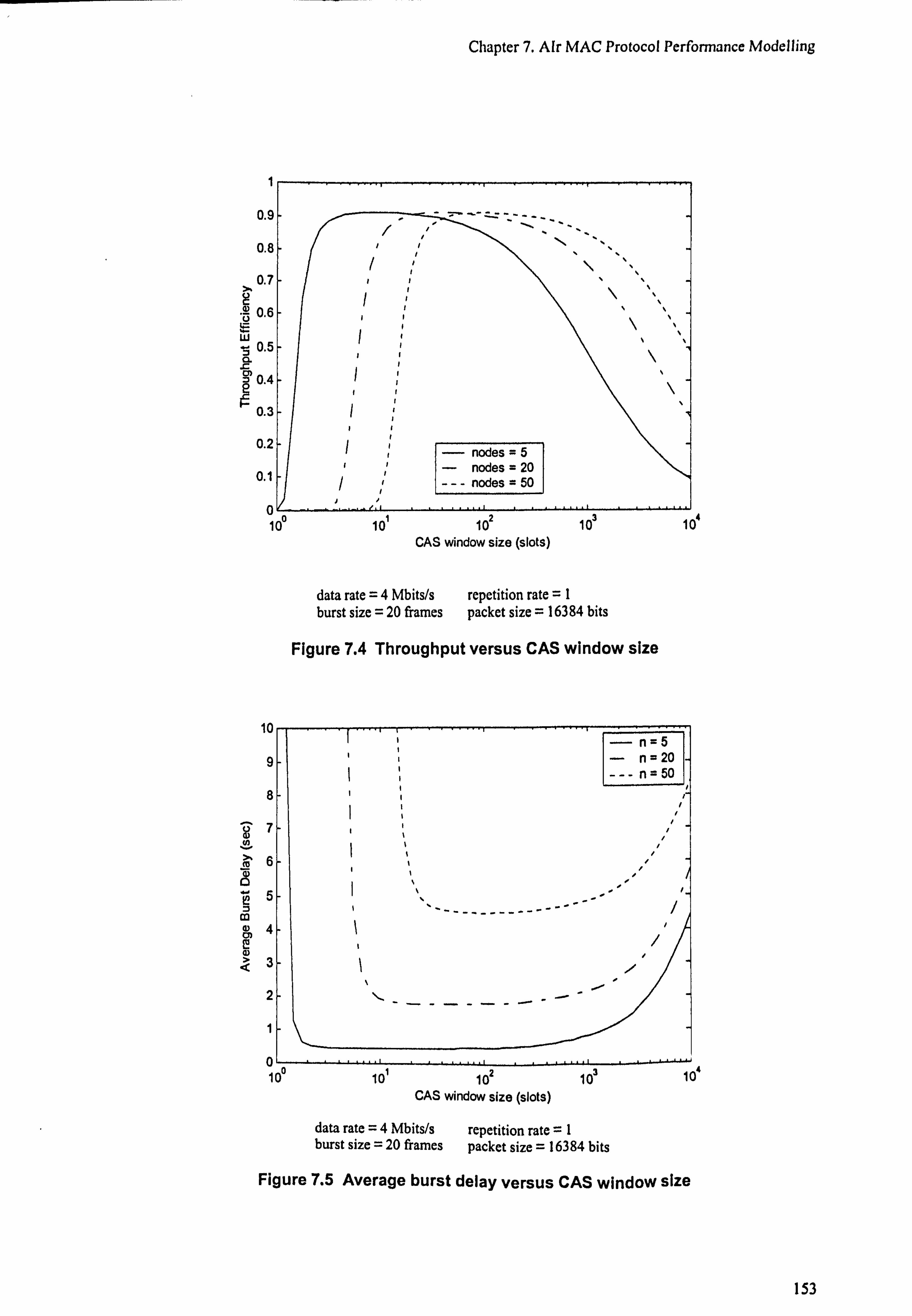
Chapter 7. Air MAC Protocol Performance Modelling
0.9 0.8
0.7 ý 0.6
ý 0.5 a s ý 0.4
0.3
0.2
0.1
/
1
i i
I
I,; �7_
r
I
I I
I
I I I
f I I I
I /,
ýý`ý_
- nodes =5 nodes = 20
--- nodes = 50
I , .
ý `.
\
ý
V1
100 101 102 . 103 104
CAS window size (slots)
data rate =4 Mbits/s repetition rate =I burst size = 20 frames packet size =16384 bits
10
i i
Figure 7.4 Throughput versus CAS window size
i i i i i i ý
I I I I I N
\ýýýýýýýýýý
IN
I
ý \ý
- n=5 - n=20 --- n=50
i
\ ^I
A
'J
ý --------...,
ý . .ý
�p ' pp ' ý.. /
/ I
e /
100 101 102 10ý 10 CAS window size (slots)
data rate =4 Mbits/s repetition rate =1 burst size = 20 frames packet size = 16384 bits
Figure 7.5 Average burst delay versus CAS window size
153

Chapter 7. AIr MAC Protocol Performance Modelling
data rate =4 Mbits/s repetition rate =1 burst size = 20 frames packet size = 16384 bits
Figure 7.6 Throughput versus number of nodes and CAS window size
data rate =4 Mbits/s repetition rate =1 burst size = 20 frames packet size = 16384 bits
Figure 7.7 Average burst delay versus number of nodes and CAS window size
154

Chapter 7. AIr MAC Protocol Performance Modelling
0.9
0.8
0.7 ý ý 0.6
w 3 0.5 a s
0.4 F-
0.3
0.2
1
Cý, ý -----------
r ý i
rI
0.1
_ WC) =4
_ Wo=32
___ Wo= 128
oý 0 5 50
Figure 7.8 Throughput versus number of nodes for ±4 CAS window back-off
3.5
3
2.5
T
2 G)
LO 7
.01.5 a) cm a) ý'a 1
data rate =4 Mbits/s repetition rate =1 burst size = 20 frames packet size = 16384 bits
Figure 7.9 Average burst delay versus number of nodes for ±4 CAS window back-off
I
ýýý I
.' ,ý _ý
I /.
---- _�S
0.5 ,'
1-1,
10 15 20 25 30 number of nodes
35 40 45
data rate =4 Mbits/s repetition rate =1 burst size = 20 frames packet size = 16384 bits
I I
ý
I I
I I ý
" ii /, I
/.
01 1I11
05 10 15 20 25 30
number of nodes
155

Chapter 7. Air MAC Protocol Performance Modelling
7.2.2 Validation of Air MAC Analysis results
Figures 7.10 to 7.13 show simulation and analytical utilisation and delay results for
validation of the results from the AIr MAC analytical model. The results are produced from the AIr network OPNET simulation model described in Appendix A. These show
a good correlation between the simulation and analytical results demonstrating a good
accuracy of the analytical model.
1 0.9
-- analysis: nodes "5 analysis: nodes " 15
-- analysis: nodes 25 A simulation: nodes 5 o simulation: nodes 15 o simulation: nodes 25
Figure 7.10 Simulation and analysis throughput versus CAS window size
Figure 7.12 Simulation and analysis throughput versus network size with CAS back-
off
0.5
0.4
0.6
0.8
0.7
0.3
0.2
0.1
0ý 0
analysis: W"8 -- analysis: W" 32
analysis: W" 128 n simulation: W 8 o simulation: W 32 Q simulation: W 128
5 10 15 20 number of nodes
25
Figure 7.11 Simulation and analysis throughput versus network size
Figure 7.13 Simulation and analysis delay versus network size with CAS back-off
30
156

Chapter 7. Air MAC Protocol Performance Modelling
7.2.3 Air MAC Unreserved Simulation Results
In the Unreserved mode, a UDATA frame is transmitted after winning contention for
the medium. There is no acknowledgement from the receiving station so the
transmitting station does not know if a collision has occurred. As such the CAS window back-off process is not possible in this mode. If a collision occurs, the other stations in
the network will not be aware that any transmission has been made and will continue to
contend for the medium. The two or more transmitting devices who collided (choose the
same CAS slot time) will continue contending for the medium when the frame
transmission has completed. This puts these stations out of synchronisation with the
other contending stations as the UDATA frame transmission time is greater than a slot time duration. Collisions can then occur when transmissions times partially overlap. Synchronisation only occurs following a successful transmission. In this case stations
hearing the start of transmission will pause the CA timer, and restart the timer when
reception of the frame has completed. Figure 7.14 shows throughput versus CAS
window size for networks sizes of 5,10 and 20 stations in unreserved mode. The
throughput initial rises with the CAS window size as the probability of collision
decreases then fall . The maximum utilisation achieved for the 5 station network in only
approximately 50%. Figure 7.15 shows the average packet delay versus CAS window
size for the unreserved mode. These demonstrate that the unreserved mode is both
unreliable (no acknowledgement) and inefficient. The CAS window size would need to
be carefully set for a particular network size to optimise the utilisation.
157

Chapter 7. AIr MAC Protocol Performance Modelling
Figure 7.14 Simulation of unreserved throughput versus CAS window size
Figure 7.15 Simulation of unreserved packet delay versus CAS window size
158

Chapter 7. AIr MAC Protocol Performance Modelling
7.3 Chapter Summary
This chapter has presented an analytical model of the AIr MAC protocol to provide
reservation mode saturation utilisation and delay in relation to the network size (number
of contending devices), contention window size and other MAC parameters. The
analysis also examines the contention window back-off process using a Markov model
of the process and concludes that the process is very effective at optimising utilisation for all network sizes. Analytical results are validated by results from an OPNET
simulation model of the AIr protocol. The simulation model is also used to produce
unreserved mode utilisation and delay results in relation to network size and contention
window size.
159

Chapter 7. AIr MAC Protocol Performance . Modelling
160
8. CONCLUSIONS AND FURTHER WORK
8.1 Summary of Thesis
An analysis of the IR wireless physical layer has provided expressions for link bit-error-
rate (BER) in relation to transmitter characteristics (output radiant intensity, radiation lobe), receiver characteristics (area, responsivity, field-of-view, bandwidth), link
distance and geometry, line modulation / encoding scheme, and ambient light power level. The effect on the link BER of third IR wireless user interference and resultant directional and spatial asymmetry have also been examined. This indicates the
minimum separation distance for independent links without cross-interference.
An analytical model of the IrDA Lx IrLAP protocol has been presented which provides
saturation condition throughput in relation to link data rate, BER and link parameter
settings of data packet size, transmission window size, minimum turn-around delay, and
maximum turn-around time. Numerical values have been provided for simultaneous
optimisation of data packet size and transmission window size for maximum
throughput. Linking of the physical layer BER to throughput analysis provides the
effective range of links and range increase with optimisation. Results from a simulation
model of the IrDA 1. x protocol validate the analytical model results and analyse non-
saturation IrLAP throughput and delay.
An analytical model of the IrDA AIr (Advanced Infrared) MAC protocol has been
presented and provides saturation condition utilisation and delay in relation to the
network size (number of contending devices), contention window size and parameter
settings of data packet size, transmission burst size and contention time slot size. The
effectiveness of the proposed contention window back-off process has been examined
using Markov analysis. Results from a simulation model of the AIr MAC process
validate the analytical model and analyse non-reservation utilisation and delay.
161

Chapter 8. Conclusions and Further Work
The main contributions to knowledge from this thesis are: 1. Derivation of expressions for accurate calculation of IrDA 1. x IrLAP link saturation
throughput from link BER, data rate and protocol settings. 2. Simultaneous optimisation values for data packet size and transmission window
size. 3. Derivation of expressions for utilisation of and delay of the IrDA AIr MAC protocol
and analysis of the effectiveness of the contention window back-off procedure. 4. Derivation of expressions for IrDA based physical layer BER in relation to
transceiver characteristics, link geometry, line encoding schemes, ambient light levels and the presence of a third user interferer.
5. Indication of minimum independent link separation through asymmetry analysis. 6. Linking of IR physical layer properties derived BER to IrLAP layer throughput.
8.2 IrDA 1. x Analysis Conclusions
Minimum Turnaround Delay. The Minimum Turnaround Delay required each time
control of the link is passed from one station to the other has been shown to be a critical factor in the link performance. The effect becomes more significant with higher data
rates as the link is turned around (after the maximum window of frames has been
transmitted) much more frequently. The delay required must cover the latency period of the receiver. Receivers can have very low latencies but at a higher manufacturing cost. There is thus a trade-off between cost and higher throughput efficiency through lower
minimum turn-around delay. A low turn-around delay will also allow a constant and
small window size to be used in the simultaneous optimisation of the packet and window size with a varying packet size optimising throughput.
Packet Data Size. The performance of an IrLAP link will generally improve with an increased packet size as a) the relative contribution of the frame overhead is reduced and b) the frequency of the minimum turn-around delay implementation is reduced. However a larger packet size becomes more susceptible to bit errors. There is therefore
a trade-off between packet size and reduced throughput through the packet error probability which results in an optimum packet size for a particular link BER. It has been shown that with a low BER in certain configurations, the optimum packet size is in
162

Chapter 8. Conclusions and Further Work
excess of the maximum specified 16384 bits (2 Kbytes). The maximum data packet size
may therefore need to be extended but may still be limited by the maximum size that
can be protected by the CRC. Using a variable packet size may also require packet
segmentation and reassemble functions at higher protocol levels.
Transmission Window Size. As with the data packet size there is a trade-off between
transmission window size and the number of frame re-transmissions due to errors. If
frame errors occur for a large window size then, as the re-transmission starts with the
first frame error in the window, a large number of frame re-transmissions may be
required. The larger the link BER value, the greater the probability will be of a frame
error occurring near the beginning of the window requiring most of the window to be
re-transmitted. As with the data packet size there is therefore an optimum transmission
window size for a particular BER.
Optimisation of Performance. It has been shown that using simultaneous optimisation
of the data packet size and window size optimises the link performance in relation to the
link BER. If the minimum turn-around delay is made small (<_ 0.1 ms) the optimised
window size can be made independent of BER and small (< 7 frames) such that the 127
frame extension may not be required. Optimisation is then provided through setting the
optimum data packet size in relation to the BER. This may be physically implemented
by inference of the BER from the current frame size and frame drop rate. In relation to
the link distance, optimisation provides a more gradual fall-off in throughput with
increasing link distance and increases the link cut-off range.
F-timer duration. The analysis of the IrLAP protocol has shown that the F-timer
duration is of significance. If the P-bit frame or returned F-bit frame from the secondary is lost, the primary must wait for the expiration of the F-timer before sending an S-
frame to re-poll the secondary. This delay can significantly affect the link throughput.
The F-timer duration should therefore be set to the minimum required to receive the F-
bit frame from the secondary for the particular application envisioned.
163

Chapter 8. Conclusions and Further Work
8.3 IR Physical Layer Conclusions
Optical Power Output: The electrical signal-to-noise ratio (SNR) increases with the
square of the received optical power. Therefore increasing the LED optical power
output can greatly increase the SNR and hence performance of the link. However there
are limits on the optical output. Power efficiency must be maintained in order to
preserve the battery life of portable IR devices. There is also a output power regulation for eye-safety limiting the maximum output intensity to 500 mW/Sr. Output power
should therefore be minimised while maintaining the required link quality.
Ambient Light: The dominant source of noise in an IR receiver is shot noise induced
by background ambient light (from both sunlight and artificial sources) in the receiver. The induced shot noise is a white Gaussian random fluctuation of the photodetector
current about its mean value. An optical filter can reduce the level of ambient light
outside of the signal wavelength band, but ambient sources can have a high infrared
content within the band. High quality optical filters can have a very narrow pass-band
with high attenuation outside the band, but with greater expense. An input electrical high pass filter in the receiver can also reduce the dc and low frequency components from the noise signal.
Receiver Bandwidth. A critical factor at the physical layer is the bandwidth of the
receiver. As the receiver noise is dominated by a white Gaussian component induced
from incident ambient light levels, the total receiver noise power increases with the
receiver bandwidth. The bandwidth needs approximately to be equal to the line data rate in Hertz so higher data rates require a higher bandwidth causing a lower SNR and hence
higher BER for the same transmitter power. Analysis of the IR physical layer has shown that there is a sharp ̀ cut-off of performance at a critical link distance. Increasing the bandwidth decreases the cut-off distance.
Link Asymmetries. It has been demonstrated that link directional and spatial
asymmetry can occur in the presence of a third user interferer. For IrDA 1. x links, there is no inherent mechanism to detect a third user interferer so the approach of the interferer will degrade the BER and hence IrLAP level throughput in the direction of
164

Chapter 8. Conclusions and Further Work
approach. The use of narrow angle transceivers can reduce the spatial asymmetry
effects. Using narrow angle transceivers with the minimum IrDA physical layer
specification allows multiple IR wireless links to be operating in very close proximity (< 0.5 m) without cross interference.
8.4 Air Analysis Conclusions
Collision Avoidance Window Size. It has been shown that the size of the CAS window
(the range from which a random number of CA slots is chosen) is significant in the
performance of the AIr network. If the CAS window is small in relation to the network
size (number of stations) then there is a high probability of collision. If a collision
occurs (when two or more stations chose the same lowest CAS value - assuming
saturated conditions), it is the next highest non-coinciding chosen slot that will succeed.
If the CAS window is large in relation to the network size then collisions are less
probable but the extra CAS slots provide an excessive time overhead which affects the
utilisation. Using a dynamic CAS window back-off process can be very effective in
dealing with this. However the CAS back-off can only be used where an
acknowledgement is returned from the destination station (e. g. the RTS/CTS exchange).
A collision is then detected by the acknowledgement timer expiring. For the unreserved
data exchange where there is no recipient acknowledgement (i. e. transmitting UDATA
frames) there is no way of determining if a collision has occurred. A fixed CAS value
must be used in such situations. For a low-cost reservation system with a fixed CAS
window, a value of 32 slots has been shown to provide good utilisation for large
networks (above 5 devices) and a value of 8 slots to provide good utilisation for small
network sizes.
Dynamic CAS Window Back-off Process. It has been shown that using the proposed
dynamic CAS window back-off process with an adjustment of ±4 slots is very effective
in optimising the CAS window size and effectively produces a throughput independent
of network size. The process parameters that may affect performance are the upper and lower limits placed on the adjustments. For example for a network of just 3 stations, the
default lower limit of 8 slots may need to be reduced to remove an excessive overhead. As stated above, the process cannot be used in the unreserved mode.
165

Chapter 8. Conclusions and Further Work
Collision Avoidance Slot Size. A default CA slot time of 800 µs is used in the AIr
specification. This was chosen to be sufficiently large to cover the time for an RTS
transmission and the beginning of a CTS reply. This prevents overlapping of reservation
attempts and covers the `hidden node' problem. However in certain situations this time
can cause an excessive overhead that can affect performance. When using the
unreserved mode, a single frame only is transmitted for each contention and a fixed
CAS window size must be used. The relative time overhead can severely impair the
performance. As there is no CTS reply in this situation, the CA slot time could be
reduced to cover the PA and Sync portions of the transmitted UDATA frame only (e. g.
200 µs).
Reservation Burst Size. It can be seen that due to the time overheads of collision
avoidance, reservation establishment and frame overheads, the efficiency the AIr
network improves with greater burst size (packets per burst). However the burst size
may be limited by the requirements of upper layer protocols.
8.5 Suggestions for Further Research
The following presents suggestion for further research related to the performance
modelling and optimisation of IR wireless systems and protocols.
8.5.1 Further IrDA Protocol Research
Dynamic Adjustment of IrLAP parameters: It has been shown in the IrDA l. x
protocol analysis that the IrLAP parameters of packet size and transmission window
size have optimum values for link throughput in relation to the link quality (BER). A
dynamic adjustment of these parameters could help stabilise the link performance in
varying noise level environments. The adjustments would need to be based on the
number of required packet re-transmissions indicated by the returned Nr field. A packet
size adjustment may require data packet segmentation and re-assembly functions for
packets from upper protocol levels which can increase the complexity of the protocol. The exact nature of the adjustment algorithms for optimum performance (e. g. linear or
166

Chapter 8. Conclusions and Further Work
exponential, parameters) can be determined experimentally. Simulation modelling of
the protocols can be useful for these experimental processes.
Modelling High Speed Extensions: In addition to the proposed 16 Mbits/s high speed
IrDA extension, it may be feasible to extend to even higher data rates such as 100
Mbits/s, which could facilitate interfacing to existing LAN architectures (e. g. 100
Mbits/s Ethernet). The possible implications of operating at such data rates would need
to be examined. For example it can be seen from the IrDA analysis that very low
minimum turn-around delay and a high receiver bandwidth would be required. For such high speeds, propagation delay may also begin to be a factor needing consideration.
Varying Noise: In the analysis of the IrDA protocol it has been assumed that the
devices used in the link are static and that the link noise level (BER) is constant. However in reality the link noise level may vary during course of data transfer. This
may be due to some physical movement of the devices involved or varying ambient light levels due to some external variance (e. g. turning on/off of lights, movement of
people). An example of a movement of devices could be the natural `sway' of hand
movement when using a hand-held computing device transmitting to fixed device.
Simulation modelling can be very useful for performance modelling of these condition
as the response to a time varying input can be simulated. However it may be difficult to
accurately simulate the varying input itself. Normally some mathematical distribution of
values is required.
Modelling LAN Interface: It may be possible using simulation to model the interaction
of the IrLAP layer with an interface to a LAN network such as Ethernet using an IrLAN
protocol model in combination with other upper IrDA protocol layers such as IrLMP
and Tiny TP.
Physical System Experiments: It would be useful to obtain experimental results of IrLAP performance against physical layer measurements (link distance, ambient light
levels, transceiver characteristics etc. ) to compare with the performance results obtained in this thesis.
167

Chapter 8. Conclusions and Further Work
8.5.2 Further Air Protocol Research
Link level and link quality performance. In the performance modelling of the AIr
protocol so far carried out, the medium is assumed error free and that all stations can
receive . transmissions from all other stations in the network. The performance has been
solely based on the media access feature of collision avoidance and media reservation.
Further research can be carried out by examining the effects of physical layer
characteristics and link noise on AIr performance. Rather than the BER of the medium
the PPM chip-error-probability (chip = single PPM slot) should be used to determine the
error allocation for variable repetition PPM encoded AIr packet segments. At the MAC
layer, this will allow the effects of hidden nodes and of packets lost due to errors in
addition to packet collisions to be examined. At the AIr LC data link layer, the
throughput of the balanced HDLC based procedures can be examined in a similar
manner to the analysis of the IrLAP protocol.
168

APPENDIX A OPNET SIMULATION MODELS
A. 1 The OPNET Modeler package
OPNET Modeler is a communication networks modelling and simulation software
package from OPNET Technologies (formerly MIL3 Inc). OPNET Modeler uses a set
of graphical hierarchical domains which reflect the structure of actual networking
systems, namely, the Network domain, the Node domain, and the Process domain, to
produce a C/C++ coded simulation model of the communications network or system.
The Network domain consists of network node objects (workstations, routers etc. ) and
network links (e. g. Ethernet lines). Sub-networks can also be used to represent an entire
network topology. Long distance networks can also be represented against a
geographical map. Data packets are transferred between nodes on the network level.
The transmission of packets across network links is controlled by pipeline-stage C/C++
coded routines. The complexity of these depends on the link type (e. g. point-to-point,
multiple access, wireless). The main functions include the assignment of transmission
and propagation delays to the packet, and the assignment of bit errors. The latter are
assigned randomly based on the link bit-error-rate ('ber') parameter value and the
packet size. There is then an error threshold at the receiver that determines the packets
acceptability. Rejected packets are simply discarded and do not reach their destination.
This simulates the action of the CRC process used in most communications systems.
Each node object in the network domain represents a node model in the Node domain.
The Node domain consists of connected process modules and link receiver and
transmitter modules. Some process modules are pre-built (e. g. queue modules and ideal
data source modules). The principal means of communication between processes in a
node is through data packets and Interface Control Information packets (ICIs), both of
which are actually C data structures. Each process module (not including pre-built
modules) in the node domain represents a process model in the Process domain. A
process model is represented as a finite state machine (FSM). Each state in the model
has an Enter and Exit execution block where C/C++ coded procedures are entered.
169

Appendix A. OPNET Simulation Models
Transitions between states have associated condition macros. The flow of control in the
process is determined by interrupt events. Theses typically constitute packet arrivals or
timer expirations. These are identified by an interrupt type and user defined code using
symbolic constants. There are two types of state used; the forced state and the un-forced
state. The process will remain in the unforced state until the next interrupt event occurs
after which it will move to the next state determined by the state-flow diagram. The
process will move immediately from a forced state once the executive blocks have been
processed. Thus only the un-forced states actually model true states of the system, while forced states are used to model transitionary processes.
The code blocks in the process domain employ an extensive library of proprietary C
functions (known as Kernel Procedures - KPs) that implement OPNET specific
procedures, in addition to standard C/C++ functions and syntax. The process is
compiled using a standard C/C++ compiler and becomes an `object' used in the
simulation. When compiling, OPNET uses the code in the execution blocks with its own header information and structure to create a single C/C++ code file for the process
object. Objects in each domain in the hierarchy can have a set of attributes that can be
modified to control the behaviour of the object. These can be set at the object level or
promoted to higher levels. Figure A. 1 demonstrates the model hierarchy from an
example Ethernet model.
Process Domain Code Block
Figure A. 1 OPNET modelling hierarchy - Ethernet model example
170
Appendix A. OPNET Simulation Models
Simulation takes place in a simulation kernel where the process objects are `linked' in
accordance with the hierarchical structure of the network. The simulation is then event driven where an event is a process interrupt and each event has a simulation time tag
association. There are two types of statistics that can be obtained from a simulation. Vector statistics are recorded as a time-value pair and are recorded from individual
events during a simulation run. It can therefore be seen how a single statistic varies during the course of the simulation. The other type of statistic are Scalar statistics which
are single values collected at the end of a simulation run. A set of simulation runs can
then be used to see how a performance measure (e. g. average throughput) varies against
some system parameter.
User models can be developed from the beginning but OPNET comes with a substantial
model library of standard network systems and protocols. These can be used as they
stand or copied and modified for the users particular requirements. An issue in running
a simulation is how long (in simulation time) to run the simulation. This depends on the
objective of running the simulation, but if some average value of a performance
measure is required (e. g. average throughput) for a scalar statistic then the simulation
needs to be long enough to `smooth out' the average value. The collection of the value intended for the end-of-simulation scalar statistic as a vector statistic during the
simulation can help determine an effective simulation time. The actual time (clock time)
that a simulation takes to complete depends on the processor speed of the host computer
and the complexity of the model. Although processes in each node may run
concurrently in simulation time, each event will still need to be processed sequentially in the host processor (Barker and Boucouvalas, 2000a).
171

Appendix A. OPNET Simulation Models
A. 2 The IrDA 1. x OPNET Simulation Model
The following presents details of the IrDA 1. x OPNET simulation model. The model is
primarily concerned with modelling the IrLAP process in the information exchange
mode. The IrLMP and higher layers of the protocol are not considered in the model.
A. 2.1 IrDA Model Network Level
Figure A. 2 shows the network level for IrDA 1. x model. The `network' consists of two
desktop computer nodes acting as Primary and Secondary devices, connected by a pair
of uni-directional point-to-point links.
----------------------------- " -------------- . -------------- ----- ý..,; --------------
Primary Secondary
--------------------------------- ---------- ------------------ --------------
Figure A. 2 IrDA 1. x network level model
Although we are modelling an IR wireless system, we are primarily interested in the IrLAP layer performance. The effects of physical layer properties are not considered in
the present model. The model simply uses fixed links with user specified `ber'
attributes. These can be set individually for the link in each direction. The link data rates are set by those of the transceivers in the node models.
172

Appendix A. OPNET Simulation Models
A. 2.2 IrDA Model Packet Format
Only S-frame and I-frame packet format are used. These constitute C data structures
that model the contents and size of the individual packet fields. The formats for the
standard IrLAP packets are as given in Tables A. 1 and A. 2:
Name Type Size (bits) BOF int 8 Address int 8 Type int 2 Nr int 3 P/F int I FCS int 16 EOF int 8
Table A. 1 IrDA S-frame packet format model
Name Te Size (bits) BOF int 8 Address int 8 Type int 1 Nr int 3 P/F int I Ns int 3 Information Packet inherited FCS int 16 EOF int 8
Table A. 2 IrDA I-frame packet format model
The sizes (in bits) of the individual fields make the total modelled packet size. This is
used in calculating the packet transmission time. The value of each field can be set and
read from within a process by suitable KPs.
A. 2.3 IrLAP Basic Model
The basic model considers saturation traffic from the primary to the secondary only
with the secondary returning S-frames only. This is used to validate the throughput and
delay results from the IrLAP analytical model. There is no requirement for the P-timer
in the primary model as data packets are continually available. The secondary is reduced
173

Appendix A. ( )I'NI: T tiiniul, ition Moxicls
in complexity to simply return S-trames and record statistics of correctly received I-
franmes (Barker and Boucouvalas, 199Kd).
A. 2.3.1 IrDA Basic Model Node Level
Figure A. 3a shows the node level for the IrDA Basic primary station model. This
consists of point-to-point transmitter (xmt) and receiver (rcv) modules, and an IrLAP
(irlap) process module. Data packets are created internally within the irlap process.
Packet streams connect the IrI. AP process with the transmitter and receiver. There is
also a statistic stream (dashed line) from the transmitter to the IrLAP process. This is
used to indicate the completion of a frame transmission on the physical link. Figure
A. 3h shows the secondary node model. This is similar to the primary except there is no
statistic link from transmitter as only S-frames are returned.
irlop
J-47-1 irlap I
ILý
-- IJ
xmt rcv
fi V ofli
a) primary b) secondary
Figure A. 3 IrDA Basic model node models
A. 2.3.2 IrLAP Basic model process level
Figure A. 4 shows the process finite state machine for the IrLAP Basic model primary
station process model. There are 5 states: initialisation (INIT), transmit (XMIT), receive
(RFCV), re-transmit (RFXMIT) and turn-around delay (TA DEL). The INIT state is
forced with the remaining states unforced.
174
\

; 11, hcn(lix A. ( )I'NI I tiiinul; ilii)n NIuilclti
(FRAME XMTD 8S wndow: 1j/DEC. _WINDOW
i ý' ý ,
k IFRAME_XMTD 6L BUFFER_SENT'ýL window> 1I/DEC WIND047-,
I1A (:: fýýllfhrýSF AOdIIRiII
ý,
JF_TIMER_EXPIRýDI (FHAMELRCVDI II7i
II; ý !:! PIRED R6IF_TIMEOUT SLINR_OKI
(FRAMEXMTD && IBUFFER_SENT)/DEC_WIF790W_
(FRAME XMTD RS BUFFER SENT 6>; window -- 1)/MA' WINDI)W
Figure A. 4 IrLAP Basic model primary station process model FSM
The process operates as follows. The initialisation (IN IT) state reads the process input
attributes and initialises variables. Procedures for- the transmission of' I-frames are
contained in the enter execution block of the transmission (XMI"I) state. For each
frame, a data packet is created and a buffer copy with the current Vs value made. The
packet is then inserted into an I-frame packet and transmitted with the Nr field set to the
current Vs value. The Vs variable is incremented (with modulus). The process then
waits for completion of frame transmission as indicated by the statistic interrupt from
the transmitter module. If the window value is greater than I, the frame is transmitted
with the P-bit unset. On completion of transmission the window value is decrenºented
(DEC WINDOW) and the process returns to the XMIT state. Note that the
DEC WINDOW operation is performed as an execution statement after the transition
condition is evaluated. This is because the action changes the value that is being
evaluated. If the window is equal to I, the fiamc is transmitted with the P-hit set, the
window returned to the maximum value (MAX WINl)OW) upon frame transmission,
and the f-timer started (scheduled self-interrupt).
11 HAME XM1D R& werhm == 1I/MAh'WINUr1W
i TA_E-: FtFiED S6, 'F_TIMEOTtT &t; NH_UM. I
(FRAME XAlrnJ
ý. iýi
175

Appendix A. ( )I'NI: T Simulation Murlcls
The process then moves to the receive (RF. (-. 'V) state. Here the process waits for either a
frame reception interrupt from the receiver input stream or expiration of the f-timer. If a
frame is received, the f-timer is stopped. The Nr value is extracted from the frame and
the frame destroyed. The process then moves to the TADEL state to wait the turn-
around delay. On completion of the turn-around delay, if the received Nr value is as
expected (Nr Vs) the process returns to the XMIT state and commences transmitting
a new window of 1-frames. If Nr is not as expected (Nr # Vs) the process moves to the
re-transmission (REXMIT) state. Here a copy packet is made of the buffer copy with
index Rs. This is transmitted in an 1-frame with the Nr field set to Rs and the Rs index
incremented (with modulus). On completion of frame transmission, if the buffer has
been transmitted (Rs _= Vs) the process moves to the XMIT if the window is not equal
to 1, to transmit new 1-frames to till the window. If the window is 1, the process moves
to the RFCV state, starts the f-timer and resets the window to maximum. If the buffer is
not transmitted (Rs # Vs) the process returns to the REXMIT state to continue re-
transmission. If the f-timer expires (self interrupt) when in the RECV state an f timer-
expired flag is set and the process moves to the TA_DEL to wait the turn-around delay.
After this delay, an S-frame is transmitted and the process returns to the RECV state.
On completion of transmission, the f-timer is restarted.
(REC/_PK && IPBfT_SET)
ý ý
1, ý, (delauM)
(RECV_PK && P©IT SET)
TA DELAY
Figure A. 5 IrLAP Basic model secondary station process model FSM
176

Appendix A. ( )I'NI I tinnul, iliuii Miulcls
The process model for the secondary station in the basic IrDi\ model is ºnuch simpler as
it just receives I-frames from the secondary, records statistics and returns an S-frame
acknowledgement after receiving the P-bit and completion ofa turn-around delay. There
is therefore just a RECV state and a TA 1)EI. state. On receiving an I-frame in tic
RE('V state, the Ns, Nr and P-hit field values and the Information field data packet are
extracted. If the Ns value is equal to the current Vr value, the Vr value is incremented
(with modulus). The size of the data packet On bits) is recorded and with the time
difference since the previous packet arrival provides the instantaneous throughput
statistic. The total bits received divided by the current simulation time provides the
average throughput statistic. If the P-bit is set, the process moves to the "1A I)I: I. state
to wait the turn-around delay. On completion of' the delay, an S-frame is transmitted
with the current Vr value in the Nr field.
A. 2.3.3 IrDA Basic Model simulation Execution
Model attributes can he set at the appropriate model level or promoted to the simulation
configuration level where multiple value sets can he assigned it' required tilt a scalar
output set (e. g. throughput versus packet size). The following provides the simulation
attributes for the IrDA basic model.
Attribute Name Type -- -Units-- Primary. irlap. I)iagnostic Boolean
Primar . irla
. Max Ta Time double seconds
Primary. irla. Min Ta Time double seconds Primary. irla. Packet Size double bits
Primar . irla-. Window Size int f ranks Primar . rcv. data rate double hits second
Primar . xmt. data rate double bits % second
Primary -> Secondary. ber double errors ! hit
Secondary -> Primary. ber double errors i bit
Table A. 3 IrDA basic model simulation attributes
The `Diagnostic' attribute is used to switch on off a diagnostIC text Output to the
console window. This provides details of the IrI . AP procedure execution events. This is
very useful in debugging the process while in development but Can slow down the
execution if not required. The following shows an example diagnostic output from the
Primary node Im a simulation run. The Figure before each event is the simulation time.
1 77

Appendix A. ( )I'NI": 'I SIIIIIIlatllln Models
ý ý" , (493.162 00) Prinnuy: (49: 1.162000) Primar"y: (493.304639) Primary: (493.447278) Primary: (494.018833) Primary: (494.0i9833) Primary: (494.019833) Primary: (494.021667) Primary: (494.022667) Primary: (494.022667) Primary: (494.165306) Primary: (494.107944) Primary: (494.45'1.800) Primary: (494.453000) Primary: (494.453000) Primary: (494.595639) Primary: (494.738278) Primary: (494_J182133) Primary: (494.11113333) Primary: (494.883333) Primary: (495.025972) Primary: (495.168611> Primary: (495.312667) Primary: (495.313667) Primary: (495.313667) Primary:
TA Delay Implcmr, nted Transmitting I frame 12,0,0, (6420)I Transmitting 1-frame [3,0,0, (6430)] Transmitting I-frame [4,0.1. (6432)] 11--timer expired TA Delay Implemented Transmitting S-frame 9-frame received [41 TA Delay Implemented Retransmitting [--frame [4,0,0, (6432)] Transmitting [-frame [5,0.0, (6437)] Transmitting I-frame [6,0.1, (6439)] S frame received [7] TA Delay Implemented Transmitting I-frame [7,0.0, (6442)] Transmitting I-frame [0,0,0, (6444)] Transmitting 1-frame [1,0.1. (6446)1 S-frame received 171 TA Delay Implemented Transmitting I-frame [2,0,0. (6449)1 Transmitting F -frame [3,0,0, (6451)] Transmitting I-frame [4,0.1, (6453)] S-frame received [5] TA Delay Implemented Transmitting I-frame [5,0,0, (6456)]
Figure A. 6 Primary station example diagnostic output
The figures in the I-frame transmission output are the Ns, Nr, P/F bit and data packet id
respectively. The figure for the received S-frame is the returned Nr value. It can be seen
that following the first transmission window shown, the I-frame [4,0,1 (6432)] which
carries the P-bit is lost. The F-timer therefore expires. The frame (6432) is re-
transmitted at the start of the next transmission window.
El 0 in 0 ý
At the secondary irlap process, the throughput and delay statistics are recorded (as time-
value pairs) for each correctly received packet. Delay is read from the creation time
stamp of each packet. At the termination of the simulation, the average throughput and
average delay are recorded together with the link BER value and parameter setting as a
scalar statistics set.
A. 2.4 IrLAP Advanced Model
The advanced model does not assume a saturated data condition but instead accepts data
requests From a packet source process. The secondary also has a full IrLAP information
translcr procedure and can return its own I-frame data packets, if available, in addition
to returning S-frame acknowledgements.
179
hL

-lhhcn(lix A. OI'NI I Simul; ilion tiliulcls
A. 2.4.1 IrLAP Advanced Model Node Level
The node levels for the advanced model clificr f'ronr the hasic model in
sink process modules are connected to the Irl. AI process. Fm- the
constant packet size is used with random delivery times.
source
irlep
niM
--,
' ---------- l-> ý 1
-tilt
I CI r(7/
that uourr. r and
IrI ), A rriouleI ýr
Figure A. 7 IrDA Advanced model primary station node model
A. 2.4.2 IrDA Source and Sink Models
The source model process Uses a Poisson distribution to schedule packet transmissions
to the irlap process at random intervals with the specified mean interarrival time.
Attributes also specify the packet size and send-data enabled disabled condition. The
sink process receives correctly received packets from the irlap process, records statistics
and destroys the packets. Throughput and Delay vector statistics are recorded fir each
packet arrival during the simulation run. At the termination of' the simulation, average
throughput and delay together with irlap and source parameter values hroni file
transmitting node are printed to the terminal output and recorded as scalar statistics.
A. 2.4.3 IrLAP Primary Station Advanced Process Model
The advanced In AP primary station model is similar to the hasic model except that the
process waits in the XM IT state for a data packet request (10-J) streu» interrupt) Iron
the packet source process unless there are packets queued in the request stre, rnn v"aiting
1 71)

. Ahhcndix A. OI'NI: 'I' Sinuilatioýn Models
transmission. If packets are waiting transmission, a frame transmission is in progress or
the process is not in the XMIT state, the REQ stream interrupt is disabled. Thus, any
arriving packets in the REQ stream are queued in the stream without an interrupt. The
P-tinier is also used in the process. It is started (scheduled self-interrupt) on entering the
XMI'I' state from any other state. The duration is set to be slightly longer than the
maximum time to transmit (N - I) sequential I-frames. If the Nth frame (frame to the P-
bit set) arrives before expiration of the timer, the timer is stopped. If the P-timer expires,
an S-dame is transmitted with the current Vr value in the NR field to poll the
secondary. 1f data packets are queued in the REQ stream, the process will sequentially
transmit the packets as with the basic model until the queue is empty.
I-frame arrivals in the RECV state from the secondary if in sequence (Ns Vr) have
the data packet extracted and passed to an external `sink' process where statistics are
collected. The Vr variable is then incremented (with modulus). If the I-frame is not in
sequence, the data packet is discarded. Other procedures (F-timer expiration, re-
transmission) are as the basic model. The advanced model primary and secondary Irl. AP unite-state diagrams are illustrated in Figures A. 8 and A. 9.
IIfRAME_XMTD && wndow > IuDEC_WINDOW
IP_TIMER_EXPIREDI
11 I
(FRAME_RLVD S5! FBIT_SETJ
IIFRAME XMTD && window == 111MAXWINDOW
IS FRAME XMTD)/MAXWINDOW
t ' \
ýý //
ý ý\\ ;ý
(DATA_RE0) TA EXPIRED S>k, IF_TIMFOUT 2 NR OF. l /i VI rrIýN.
(FRAME _RCVD i
FBIT_SETJ .`r `
``\
f
IIFRAME_XMTD 65 BUFFER_SEN1'V window > 11/DEC_WINDOW-, (TA_EXNRED F 11MEOUT)
- __ ý.
(1n. EXPIRED E61F_TIMEOUT && INR_01 I
IIFRAMF_XMTD && iBIJFFER_SENTJIDEC_WINßQW
IIFRAME_XMTD && BUFFER-SENT && window == 1 I/MAXWINDOW
Figure A. 8 IrLAP advanced model primary station process model FSM
'ýý ýI
lý
ii ýý
\i1
JSFRAME_XMTDI
180

A( )I'ti1 I 'ý, iniul"iliun NimIrk
lflbV+d1 - MIh? Y. Nnufiýv+1I1111 ':; INlýil1
i
r
IfRAMERCVI) bbIPBIT SETI
i
ffRAME r: Ml[jl
jSFRAMF XMTh)/MAkWINOOW
IIFRAME _:
iMTU L6 window -- 1I/MAkWINhiJ',
! (TAEXPIRED NýNHUf 7, rUAL\ WN11Nld IIRArÄE'RCVä66PBIT-SET(
(IFRAME_XMTD8&BUFFER_SA'TS8DAlA_WAITINGS&1vlndow>tI/DEC_WINDUW 11 1
ý ,.. .,..,.,, ý... _ .. ý ý.. ....,... ! ...... __.
I fA_E'r<PIHk D 6R iNH_Uý I
(IFRAME_XMTD SS IBUFFER_SENT)/DEC_CV+NIlIýW
(IFRAMF XMTD && BUFFER_SENT 6S (window == I II IDATA_WAIIINGII/MAkWINDOW
Figure A. 9 IrLAP advanced model secondary station process model FSM
The secondary advanced model operate as the primary except that it will not wait in the
XMIT state for packet arrivals in REQ steam. It will only transmit data packets if they
are waiting transmission (queued in the REQ stream). Ifthe queue is empty, the process
will return the RECV state to wait I-frame arrivals from the primary. It' the queue
becomes empty following packet extraction from the RI-J. ) stream, the I-1ranne is sent
with the P-hit set regardless of remaining frame slots in the window. The secondary also
does not hold P or F timers.
A. 2.4.4 Advanced Model Simulation Execution
The behaviour of the advanced simulation model depend on the link 1311,8, Irl_; Al'
process parameters and the new parameter ol' the source packet service time. For large
service tine values, the throughput will he reduced as the process is not at , aturation
level. Beyond a certain value, the packets will queue in the input stream to the Irl AI'
process and the throughput will he that of the saturation condition. The saturation point
will depend on the link 13FR. It' packet errors occur, requiring re-trarlsillissloils, new
packet arrivals will queue up during the re-transmission period.
ix1 I

Appendix A. OI'NI-, T Simulation Models
t3 11
ý I') . '26SN2'. (11)_2616_f4i (19.2.63734> (19.264187) (19.285440) (19.288406) (19.208406) (19.289684) (19.289'184) (19.291534) (19.295646) (19.299758) (19.307676) (19.314456) <19.314456> (19.314588) (19.314688) (19.314688) (19.343472) (19.343472) (19.343604) (19.343704) (19.343704) (19.372488) <19.372488) (19.372620) (19.372720) (19.372720) (19.376832) (19.380944) (19.385056) <19.389168> (19.393200) (19.397392) (19.401620)
l r. uI". 1t my :. f rru" I'r iIl r-SI rant. rrr. c ivrd I'. I Primary: TA Delay Implemented Primary: Transmitting I-frame IS, 0,0, <5099)] Primary: Transmitting I-frame [6.0,0. <5101)1 P-Timer Expired Transmitting S-frame 10 11 Primary: S-frame received [7 11 Primary: TA Delay Implemented Primary: Transmitting I-frame [7,0,0, (5105)] Primary: Transmitting I frame [0,0,0, (5107)] Primary: Transmitting I-frame [1,0,0, (5108)] Primary: Transmitting I-frame [2,0,0, (5111)] P-Timer Expired Transmitting S-frame CO 11 Primary: S-frame received [2 11 Primary: TA Delay Implemented Primary: Retransmitting I-frame [2,0,0, (5111)] P--Timer Expired Transmitting S-frame [0 1] Primary: S-frame received [2 1] Primary: TA Delay Implemented Primary: Retransmitting 1--frame [2,0,0, (5111)] P-Timer Expired Transmitting S-frame [0 1] Primary: S-frame received [3 11 Primary: TA Delay Implemented Primary: Transmitting I-frame 13,0.0. (5116)] Primary: Transmitting I-frame [4,0,0, (5117)] Primary: Transmitting I-frame [5,0.0. (5118)] Primary: Transmitting I-frame [6,0.0. (5122)] Primary: Transmitting I-frame [7,0,0, (5123)] Primary: Transmitting [-frame [0,0,0, (5124)] Primary: Transmitting I-frame [1,0,1, (5130)] Primary: S-frame received 16 1]
_Qx
71
Figure A. 10 Non-saturation advanced IrDA model diagnostic output
A. 3 Air OPNET Model
The following presents a description of the Alr OPNET simulation model. The basis of
the model is principally to simulate the behaviour of the Air MAC process. As such we
are interested in how the media reservation process and packet collisions affect the
performance rather than the effect of bit errors (Barker and Boucouvalas, 2000b; Barker
et al., 2002).
A. 3.1 Air Model Network Level
Figure A. I I shows a 5-station scenario network level for the Air OPNET model. In
addition to the Air node stations there is a monitor station the records statistics on
network traffic. Other network scenario models were produced for different network
sizes (e. g. 10,15,20 stations etc. ).
182

\I)I)cn(lix A. ( )I'NI I ýIlllul; lllml tilmIcls
�noh ,
,b
11, I.: .
nude 4
Figure A. 11 Alr model 5-stat'jon network level
The model is actually implemented as a 'radio' wireless network with certain
modifications to the pipeline stages to model the behaviour of the Air IR wireless
physical layer. Infrared as a wireless medium is not as yet supported by OPNN. T
Modeler, but as we are primarily concerned with the AIr MA(' protocol behaviour, the
radio medium can be used with some modifications. The principal change was to have
nodes unable to 'hear' their own transmissions while ensuring that packet collisions
would cause appropriate errors in the relevant packets. With the 'radio' inedium tile
BER is not specified as an attribute as is the case with wired network links hut is
determined from link distances and transmitter, receiver and antenna model attributes.
With a multiple access medium such as the 'radio' nmedium, a transmitted packet is
duplicated and sent to each receiver on the network. Pipeline stages are used fi, r each
destination to determine a packets error and acceptability. In the current model we are
primarily considering an error free situation with no hidden nodes' so the network
model was modified to remove all packet errors. Ilowever future modifications to the
model could easily be made if'a single BER value fir- the network was required or errors
to be calculated form link geometry and transceiver characteristics.
18 3

nhpcndix A. c>l'wý; ýr Simulation Nllxlcls
A. 3.2 Air Station Node Model
Figure A. 12 shows the Alr station node model. This consists of `radio' transceiver
modules, an AIR E NY physical layer interface module, the AIr MAC process module
and the Ah- LM module. The LM module acts as a data source / sink and management
client to the MAC layer in this model. The LC process was not included in the current
model.
LM
MAC
--- ----ý ý. __.. AIR_PHY
rcv
----- -------'-ý H
h,.
xmt
Figure A. 12 Air station node model
A. 3.3. Air LM Process Model
Figure A. 13 shows the Air LM process FSM. The process here acts as a reservation
client to the Air MAC process and as a data source and sink. The procedures for
intent icing with the MAC is not fully developed in the LM draft specification document
and as such the process here is some what different from that in the LM specification.
184

Appendix A ()I'NI" I ýIII111I; It1o11 NliuIck
(default]
(END-RES) 'x , 1'ý
Idelaulll
i, ý IRES_ESIABLISHEDI
Figure A. 13 Air LM process model FSM
Of particular importance is the responsibility of the IN to generate the ('AS values for
the MAC. The model uses a set of input attribute values to control the ('AS algorithnm.
These are: minimum CAS window, maximum CAS window, ('AS window increase
value, CAS window decrease value. A retry limit of 5 is used in the model and so the
CAS value vector (array) has 5 values. The ('AS window I'm- the kth element in the
array (0 to 4) is:
cas_window[k] = min(max_cas_window, init__cas window + k"cas window increase)
The CAS values are then created by:
cas[k] = floor(op_dist_uniform(cas _window[k]))
where 0/) dis/ rmif r°m is an Opnet procedure that returns a random valuc from a
uniform distribution between O and the given argument value. When the reservation has
completed, the retry count is returned to the I. M. This is used to adjust the initial (', 1S
window by:
Ihý-N

nhhcnclix A. 0I'NF. '1' Sinurl, rtion Moxlcls
finit -cas window = max(min_cas_window, cas_window[retry_count] - cas_window_decrease)
If the retry limit is reached and hence the MAC process returns a failed reservation, the
initial ('AS window value becomes:
finit cas_window = cas_window[retry_limit]
The station destination address for each reservation is chosen randomly from the
network size detected, ignoring the nodes own address and that of the monitor station. A
nodes devices address is taken from the `object id' that is assigned by the simulation
kernel to every object in the simulation. The LM process also acts as a data sink to
received packets and collects performance statistics. The statistics collected here, as
opposed to those at the monitor node, are for end-to-end performance above the MAC
layer.
A. 3.4 Air MAC Process Model
Figure A. 14 shows the process level FSM for the Air MAC protocol. The FSM is
closely based on that laid out in the specification. However procedures for DATA and
UDATA data frames only have been implemented. The procedure for transmitting
DATA frames can be summarised as follows. After initialisation in the INIT state where
process attribute values are read, the process moves to the IDLE state. A setup-
reservation-request primitive is passed from the LM to the MAC' and consists of a
`chain' of data packets together with an ICI containing parameter values for the
reservation. This includes the array of CAS values created by the LM. Each data packet
in the chain also has its own ICI containing parameter values relevant to the packet. The
packet chain consists of an empty `holder' packet with the data packets inserted as
numbered fields. The CA (collision avoidance) timer is started (scheduled self-interrupt)
using the I" value in the CAS array. The process then moves to the CONTEND state.
The process then proceeds as defined in chapter 4.
186

Appendix A. ()I'NI 'I' tiinnil, ilioi 11ýýýIrlti
li,
Ili
Figure A. 14 Air MAC process model FSM
A. 3.5 The Air Physical Layer Interface Process Model
,I
The individual components of the Alr MAC frame (i. e. preanmble, Sync, Robust I leader,
and Main Body fields) are transmitted as separate packets on the medium. This is
because the arrival of each frame portion triggers a separate event in the process. The
size of the main body packet is multiplied by the RR value tier the frame bet()re
transmission.
A. 3.6 The Air Monitor Node and Process Models
The monitor node consists of a single receiver and a monitor process module. ]'he
monitor process accepts only main body packets from data carrying, frames. These are
used to the measure the throughput on the network. As the IrI)A sink process,
instantaneous and average throughput are recorded. Required attribute values Iron other
nodes are also recorded tOº- scalar statistics.
187

Appendix A. OPNET Simulation Models
A. 3.7 Air Model Attributes and Statistics
The following table provides the attribute set for each node in the network.
Attribute Type Ph . dia nostic Boolean LM. burst size int LM. min CAS window int LM. max CAS window int LM. packet size int LM. repetition rate int LM. reservation time double LM. send data Boolean LM. diagnostic Boolean LM. up CAS adjust int LM. down CAS adjust int MAC. diagnostic Boolean
Table A. 4 Air node attribute list
The attributes representing system parameters are defined at the LM process. Optional diagnostic output is used here as with the IrDA model. For the AIr model the name of each node is appended to the front of each output string to the determine the diagnostic
origin. An example diagnostic output from the AIr MAC OPNET model is shown in Figure A. 15.
#. I-
8488> nodorf IRL;, lcetu0 8oaorwotion roYwot Ma . 7114488) made-] MCI CONTEND Timor Started. time i
0.748488) nedol -Cl CA Timor Started. time to 0.0 0.748514) node_@ MCI CAD 0.740514) node_8 MCI CA Timor Pauoad. remainder "9.740544)
modem MCI CAD 0.748544) nodal MCI CA Timor Paused, remainder e 8.710511) nede_3 MCI CBD 9.71B5M) node-3 MCI Timor Paused. remainder e 0.740544) node_4 MCI
CAD
9.7414544> nuds_1 MCI CA Timer Paused. remainder 9.748584) nods_0 MCI CSC 9.749584) model MCI CBC 0.740584) nods-3 MCI CSC 0,749584) node_1 MCI CSC 0.7414712) neds_8 MCI RHR(ATR. (76.0.590809,1)) 0.719712) nods-0 MACS media statue indication. code 6.748712) nodal MCI RHR(RTS. (76,9.500880.1)) 0.740712) nodal MCI media status indication, code 9.74@712) medal MCI RHR(RTS, (76.9.500000.1)) 0.740712) nod s_3 MCI media status indication. code 9.740712) meds_4 MCI RHR(RTS. (76.0.500000.1)) 0.718712) nods_4 MCI media status indication. code 0,710724) nedol MCI FTC 0.740724) modo-2 MCI 14PCTS Timor Started. time is 6.748724) nedeMCI MBR(RTS. (76.9.5981400.1). C 0.748724) nedsý MCI WPDATAN Timor Started, time i 0.718724) nodal MCI MBR(RTS. (76.9.698000.1). ( 0.740724) nods_S MCI WPDATAN Timor Started. time i 0.746724) nods_3 MCI MBR(RTS. (76,9.680000,1>. C 8.740724) model C. 14PDATRN Timer Started. time i 0.740724) node_4 Cl MMBR(RTS. (76.8.589088.1), ( 8.740724) node-4 MCI TA Timer Started. time is 0.8 0.740924) nods-4 MCI T6 Timer Expired 0,710924) nods-4 MCI sending CTS (76.8. Sä0008) fr 0.740988) node_I MCI CAD 6.740989) model MCI CAD 8.740988) nods-2 MACS CAD 0.740988) nods-3 MCI CAD 11.741929) nods_@ MCI CAC
toad . _0 MRCI media status indication. code is 12
nodal MRCI RHR(RTS. (76.0.500800.1)) nodal MACI media status indication, cods is 12 nedsl MRCI RHR(RTS, (76.0.508000.1)) mod s_3 MACI media status indication, cods is 12 m. de_4 MACI RHR(RTS. (76.0.500008,1)) nods-4 MRCt media status indication, cods is 12 nede_2 MRCc FTC aods-2 MAC, WPCTS Timor started. time is 0.000556 nods-0 MRCI MDR(RTS. (76.9.688080.1). (76)) neds_0 MRCI WPDRTRN Timer Started, time is 0.088064 nodal MRCt MHR(RTS. (76.0.608008.1). (76)) neds3 MACI WPDRTRN Timer Started, time is 0.800064 mods MRCI MRR(RTS. (76.0.680800,1>. (76)) nodal MAC- BPDRTRN Timer Started. time is 0.088664 nod e_4 MRCt MUR(RTS. (76.0.5881128.1), (76)) nods_4 MAC, TA Timer Started, tams is 0.802288 nods _4
MAC, TA Timer Expired nods-4 MRCI sending CTS (76,0.500008) frame nods_H MACS CUD nodal MAC' CCD nods 2 MACI CCD mods-3 MACI CCD nods-0 MACI CCC
Figure A. 15 Example AIR OPNET MAC model diagnostic output
. tan Naaaraatºan rnawat Maa1Va CONTbiD Ti., Ct. rt. a. tiwý is 6.86188M CA Timr Startal. tim to 8.824888 CAD CADTiwsr
CA Tim., CAD CA Ti/wp CAD CA Tiw. r CAC
Paused,
Paused,
Paused,
Paused.
remainder - 0.991688
remainder - 0.904989
remainder - 0.824090
remainder - 0.987289
J
188

APPENDIX B Limiting Distribution of a Markov Chain
A Markov chain is a discrete time, discrete state process in which the future behaviour
of the process is dependent only on the current state and not its state history. If the
probability of transition between states is known (may be zero for some transitions), a state transition matrix P can be formed consisting of transition probabilities pij (the
probability of transition from state i to state j), defined as:
pii = P(Xn+1 = .%1 Xn = i) (B. 1)
whereXQ is the process state at discrete time n. This is the ̀ 1-step' transition probability. For n steps pu(n) is defined as:
pi (n) P(Xm+n - JIXm = t)
Using the theorem of total probabilities gives:
p (m + n) _Zp; k (m)pk; (n) k
(B. 2)
(B. 3)
Letting P(n) be the transition probability matrix for n steps, consisting of elements pu(n) from (B. 3) we get:
P(n) = P" (B. 4)
It is a property of finite state Markov chains that as n --ý oo, all rows of the matrix P"
converge towards a common limit.
189

The limiting distribution for the Markov chain is the vector of probabilities vj such that:
v= limp/(n
Applying the normalisation condition gives:
ývj =1 !
i. e. the sum of all state probabilities in v is 1.
The limiting distribution vector v is therefore found from:
V=v. P
In other words, v is a vector such that v times (using matrix multiplication) the one-step
probability matrix P results in same vector v. This provides a set of simultaneous
equations, which together with the normalisation condition, provide a solution for v.
190

Appendix C Gaussian Tail Integral, Q- function
The function Q(z), defined in (C. 1), provides the area under the tail of a Gaussian curve from the point z forward (shaded area Figure C. 1). It therefore provides the probability
that a random outcome with a Gaussian distribution, with mean value u and standard
deviation a exceeds the value (u + az).
I ý Q(Z) = r-
5e2I2dy
7C Z
(C. 1)
This can also be determined from the erfc function (conjugate error function -
commonly included in the maths library of programming languages).
Q(z)=2erfc (-,
(2-)
lu Z
(C. 2)
a
Figure C. 1 Area under Gaussian curve tail Figure C. 2 Plot of Q(z) versus z
191

192
References [1] AGILENT, 2000. IrDA Data Link Design Guide. Agilent Technologies
[2] AIMES, G. T. AND LAZOWSKA, E. D., 1979. The Behaviour of Ethernet-Like Computer Communications Networks. In: ACMSIGCOM 7th International Symposium on Operating System Principles, Asilomar, CA, 1979,66 - 81.
[3] ALDIBBIAT, N. M., GHASSEMLOOY, Z. AND MCLAUGHLIN, R., 2001. Performance of Dual Header-Pulse Interval Modulation (DH-PIM) for Optical Wireless Communications Systems. Proceedings of the SPIE, 4214(February 2001), 144 -152.
[4] ALVAREZ, J. R. V., HERNANDEZ, F. J. L., GALDON, A. S., JIMENEZ, R. P. AND BORGES, J. A. R., 1999. Infrared Wireless DSSS System for Indoor Data Communication Links. Proceedings of the SPIE - The International Society for Optical Engineering, 3850,92 - 99.
[5] ANANTH, R., NOLL, M. AND PHANG, K., 1997: Low-Voltage Infrared Transceiver Design. Communications Systems Design, (October 1997), 52 - 61.
[6] AUDEH, M. D. AND KAHN, J. M., 1995. Performance Evaluation of Baseband OOK for Wireless Indoor Infrared LAN's Operating at 100 Mb/s. IEEE Transactions on Communications, 43(6), 2085 - 2094.
[7] AUDEH, M. D., KAHN, J. M. AND BARRY, J. R., 1996. Performance of Pulse- Position Modulation on Measured Non Directed Indoor Infrared Channels. IEEE Transactions on Communications, 44(6), 654 - 659.
[8] BAKALIDIS, G. N., GLAVAS, E. AND TSALIDES, P., 1996. Optical Power Distribution in Wireless Infrared LANs. lEE Proceedings Communications, 143(2), 93 - 97.
[9] BARKER, P. AND BOUCOUVALAS, A. C., 1998a. IrLAP Protocol Performance Analysis of IrDA Wireless Communications. Electronics Letters, 34(25), 2380 - 2381.
[10] BARKER, P. AND BOUCOUVALAS, A. C., 1998b. Performance Analysis of the IrDA Protocol in Wireless Communications. In: First International Symposium on Communications Systems & Digital Signal Processing, Sheffield Hallam University - UK, 6-8 April 1998, Sheffield Hallam University Press, 6- 10.
[I I] BARKER, P. AND BOUCOUVALAS, A. C., 1998c. Performance Modelling of the IrDA Protocol for Infrared Wireless Communications. IEEE Communications Magazine, 36(12), 113 - 117.
[12] BARKER, P. AND BOUCOUVALAS, A. C., 1998d. A Simulation Model of the IrDA Infrared Communications Protocol. In: First International Symposium on
193

Communications & Digital Signal Processing, Sheffield Hallam University - UK, 6-8 April 1998, Sheffield Hallam University Press, 2-6.
[13] BARKER, P. AND BOUCOUVALAS, A. C., 2000a. Modelling of the IrDA and AIr Wireless Infrared Communications Protocols. In: 1st Annual PostGraduate Symposium on the Convergence of Telecommunications, Networking and Broadcasting (PGNET 2000), Liverpool John Moores University, 19 - 20 June 2000,137 - 142.
[14] BARKER, P. AND BOUCOUVALAS, A. C., 2000b. A Simulation Model of the Advanced Infrared (AIr) MAC protocol using OPNET. In: 2nd International Symposium on Communication Systems, Networks and Digital Signal Processing (CSNDSP 2000), Bournemouth University, 18 - 20 July 2000,153 - 156.
[15] BARKER, P. AND BOUCOUVALAS, A. C., 2002a. Directional and Spatial Asymmetry in IrDA 4PPM Infrared Wireless Links with Third User Interference. In: 3rd Annual PostGraduate Symposium on the Convergence of Telecommunications, Networking and Broadcasting (PGNET 2002), Liverpool John Moores University, 17 - 18 June 2002,353 - 358.
[16] BARKER, P. AND BOUCOUVALAS, A. C., 2002b. Interference Induced Asymmetry in IrDA 4PPM Infrared Wireless Links. In: 3rd International Symposium on Communication Systems, Networks and Digital Signal Processing (CSNDSP '02), University of Staffordshire, 15 -17 July 2002,479 - 482.
[17] BARKER, P., BOUCOUVALAS, A. C. AND VITSAS, V., 2000. Performance Modelling of the IrDA Infrared Wireless Communications Protocol. International Journal of Communications Systems, 13(7-8), 589 - 604.
[18] BARKER, P., VITSAS, V. AND BOUCOUVALAS, A. C., 2002. Simulation Analysis of the advanced infrared (AIr) MAC wireless communications protocol. IEE Proceedings Circuits, Devices and Systems, 149(3), 193 -197.
[ 19] BARRY, J. R., 1994. Wireless Infrared Communications, ed. Kluwer.
[20] BARRY, J. R. AND KAHN, J. M., 1995. Link Design for Non-Directed Wireless Infrared Communication. Applied Optics, 34(19), 3764 - 3776.
[21] BARRY, J. R., KAHN, J. M., LEE, A. E. AND MESSERSCHMITT, D. G., 1991a. High Speed Nondirective Optical Communication for Wireless Networks. IEEE Network Magazine, November 1991,44 - 53.
[22] BARRY, J. R., KAHN, J. M., LEE, E. A. AND MESSERSCHMITT, D. G., 1991b. Simulation of Multipath Impulse Response for Indoor Diffuse Optical Channels. In: IEEE workshop on wireless local area networks, Worcester MA, May 1991,81 - 87.
[23] BEALE, M., 1999. Optimizing the High-Speed IrDA Extensions. Electronic Engineer, (August 1999).
194

[24] BEALE, M., 2000. Understanding the High-Speed Extensions to IrDA. In: IN International Conference and Exhibition, Taipei, Taiwan, 3-4 May, 2000,67 - 70.
[25] BI, Q., ZYSMAN, G. I. AND MENKES, H., 2001. Wireless Mobile Communications at the Start of the 21st Century. IEEE Communications Magazine, 39(1), 110-116.
[26] BIANCHI, G., 1998. IEEE 802.11 - Saturation Throughput Analysis. IEEE Communications Letters, 2(12), 318 - 320.
[27] BIANCHI, G., 2000. Performance Analysis of the IEEE 802.11 Distributed Coordination Function. IEEE Journal on Selected Areas in Communications, 18(3), 535 - 547. .
[28] BIANCHI, G., FRATTA, L. AND OLIVERI, M., 1996. Performance Evaluation and Enhancement of CSMA/CA MAC Protocol for 802.11 Wireless LANs. In. 7th International Symposium on Personal, Indoor & Mobile Radio Communications (PIAMC '96), Taiwan, 15 -18 Oct 1996,392 - 396.
[29] BOUCOWALAS, A. C., 1996. Indoor Ambient Light Noise and its Effect on Wireless Optical Links. lEE Proceedings on Optoelectronics, 143(6), 334 - 338.
[30] BOUCOUVALAS, A. C. AND BARKER, P., 2000. Asymmetry in Optical Wireless Links. IEE Proceedings in Optoelectronics, 147(4), 315 - 321.
[31] BOUCOUVALAS, A. C., JERRAMS-SMITH, J. AND HEATHCOTE, D., 1996. Interference Induced IR Link Spatial Asymmetries. In: Third Communication Networks Symposium, Manchester Metropolitan University, 8 -9 July 1996,214 -219.
[32] BOUCOUVALAS, A. C. AND VITSAS, V., 2001. Optimum Window and Frame Size for IrDA Links. Electronics Letters, 37(3), 194 - 196.
[33] BREWSTER, R. L. AND GLASS, A. M., 1987. Throughput Analysis of Non- persistent and Slotted Non-persistent CSMA/CA Protocols. In: 4th International Conference on Land Mobile Radio, Coventry, UK, 1997,231 - 236.
[34] BUCHANAN, W., 1996. Applied Data Communications and Networks, ed. Oxford: Chapman & Hall.
[35] BURAKOWSKI, W., BURSZTYNOWSKI, D. AND LUBACZ, J., 1986. Protocol HDLC-ABM: Traffic Considerations Given Error Dependent Channel. In: Kuhn, P. Ed, North-Holland: Elsevier Science Publishers, 549 - 554.
[36] BUX, W. AND KUMMERLE, K., 1980. Balanced HDLC Procedures: A Performance Analysis. IEEE Transactions On Communications, com-28(11), 1889 - 1898.
195

[37] CARLSON, D. E., 1980. Bit-Oriented Data Link Control Procedures. IEEE Transactions on Communications, COM-28(4), 455 - 467.
[38] CARRUTHERS, J. B. AND KAHN, J. M., 1997. Modeling of Nondirected Wireless Infrared Channels. IEEE-Transactions-on-Communications., 45(10), 1260 - 1268.
[39] CHAN, H. -H., ELMIRGHANI, J. M. H. AND CRYAN, R. A., 1996. Performance Analysis of Indoor Infrared Wireless Networks Utilising PPM CDMA. In: IEEE International Conference on Communications. Converging Technologies for Tomorrow's Applications. ICC 96, Dallas, TX, USA, 23 - 27 June 1996, IEEE, 1467 - 1471.
[40] CHAN, W. C., 2000. Performance Analysis Of Telecommunications and Local Area Networks, ed Kluwer.
[41 ] CHHAYA, H. S. AND GUPTA, S., 1997. Performance Modeling of Asynchronous Data Transfer Methods of IEEE 802.11 MAC Protocol. Wireless Networks, 3(3), 217 - 234.
[42] CHOW, F. M. AND KAHN, J. M., 1999. Effect of Non-reciprocity on Infrared Wireless Local-Area Networks. In: IEEE Global Communications (GLOBECOM'99), Rio de Janero, Brazil, 5-9 Dec 1999,330 - 338.
[43] CHU, T. S. AND GANS, M. J., 1987. High Speed Infrared Local Wireless Communication. IEEE Communications Magazine, 25(8), 4- 10.
[44] CROW, B., WIDJAJA, I., KIM, J. G. AND SAKAI, P., 1996. Performance of IEEE 802.11 Wireless Local Area Networks. Proceedings of the SPIE, 2917,480 -491.
[45] CROW, B. P., WIDJAJA, I., KIM, J. G. AND SAKAI, P. T., 1997. IEEE 802.11 Wireless Local Area Networks. IEEE Communications Magazine, 35(9), 116 - 126.
[46] DESIMONE, A. AND NANDA, S., 1995. Wireless Data: Systems, Standards, Services. Wireless Networks, 1(3), 241 - 253.
[47] DJAHANI, P. AND KAHN, J. M., 2000. Analysis of Infrared Wireless Links Employing Multi-beam Transmitters and Imaging Diversity Receivers. IEEE Transactions on Communications, 24(12), 2077 - 2088.
[48] ELMIRGHANI, J. M. H. AND CRYAN, R. A., 1994. Indoor Infrared Wireless Networks Utilising PPM CDMA. In: Ng-CS AND Yeo-TS Eds. Singapore ICCS 94. Conference Proceedings, Singapore, 1994, IEEE, 334 - 337.
[49] FIORINI, D., CHIANI, M., TRALLI, V. AND SALATI, C., 1994. Can We Trust in HDLC. ACMSIGCOMM- Computer Communications Review, 24(5), 61 - 80.
196
[50] FLOREZ, S. A. J., HDEZ, F. J. L., GALDON, A. S. AND ALVAREZ, J. R. V., 1997. Infrared Wireless Indoor Channels Characterisation in Asymmetrical Rooms. In: 1997 SBMO/IEEE M7T-S International Microwave and Optoelectronics Conference. 'Linking to the Next Generation. Natal, Brazil, 11 - 14 Aug 1997, IEEE, 492 - 497.
[51] GAGLIARDI, R. M. AND SHERMAN, K., 1995. Optical Communications, 2nd ed. Wiley. .
[52] GAMEIRO, A. AND ALVES, R., 1999. Coding Techniques for Wireless Infrared Communications. Proceedings of the SPIE - The International Societyfor Optical Engineering., 3532,70 -81.
[53] GARCIA-ZAMBRANA, A. AND PUERTA-NOTARIO, A., 1999. RZ-Gaussian Pulses Reduce the Receiver Complexity in Wireless Infrared Links at High Bit Rates. Electronics-Letters, 35(13), 1059 - 1061.
[54] GEORGES, J. AND WYBAUX, D., 1981. A Simulation Study of the Performances of HDLC Controlled Links. Performance Evaluation, (1), 126 - 138.
[55] GEORGHIADES, C. N., 1994. Modulation and Encoding for Throughput-Efficient Optical Systems. IEEE Transactions on Information Theory, 40(5), 1313 - 1326.
[56] GERALD, C. F. AND WHEATLEY, P. 0., 1999. Applied Numerical Analysis, 6th ed MA: Addison-Wesely.
[57] GFELLER, F. AND HIRT, W., 1998. A Robust Wireless Infrared System with Channel Reciprocity. IEEE Communications Magazine, 36(12), 100 - 106.
[58] GFELLER, F., HIRT, W., DE-LANGE, M. AND WEISS, B., 1996. Wireless Infrared Transmission: How to Reach all Office Space. In: 1996 IEEE 46th Vehicular Technology Conference. Mobile Technology for the Human Race, Atlanta, GA, USA, 28 Apr -1 May 1996, IEEE, 1535 - 1539.
[59] GFELLER, F. R. AND BAPST, U., 1979. Wireless Communication via Diffuse Infrared Radiation. Proceedings of the IEEE, 67(11), 1474 - 1486.
[60] GHASSEMLOOY, Z., HAYES, A. R. AND SEED, N. L., 2001. The Effect of Multipath Propagation on the Performance of DPIM on Diffuse Optical Wireless Communications. In: LASTED conference on wireless and optical communications, Canada, June 27 - 29 2001,166 - 172.
[61] GHASSEMLOOY, Z., HAYES, A. R., SEED, N. L. AND KALUARACHCHI, E. D., 1998. Digital Pulse Interval Modulation for Optical Communications. IEEE Communications Magazine, 36(12), 95 - 99.
[62] GLASS, A. M., BREWSTER, R. L. AND ABDULAZIZ, N. K., 1988. Modelling of CSMA/CA Protocol by Simulation. Electronics Letters, 24(11), 692 - 694.
197

[63] GUMMALLA, A. C. V. AND O'LIMB, J., 2000. Wireless Medium Access Control Protocols. IEEE Communications Surveys, 2- 15.
[64] HARRISON, P. G. AND PATEL, N. M., 1993. Performance Modelling of Communication Networks and Computer Architecture, ed. Addison-Wesley.
[65] HAYES, A. R., GHASSEMLOOY, Z. AND SEED, N. L., 1999. Optical Wireless Communication using Digital Pulse Interval Modulation. Proceedings of the SPIE - The International Society for Optical Engineering, 3532,61 - 69.
[66] HEATLY, D. J. T., WISELY, D. R., NEILD, I. AND COCHRANE, P., 1998. Optical Wireless: The Story So Far. IEEE Communications Magazine, 36(12), 72 - 82.
[67] HIGGINBOTTOM, G. N., 1998. Performance Evaluation of Communication Networks, ed. Norwood, MA: Artech House.
[68] HIRT, W., HASSNER, M. AND HEISE, N., 2001. IrDA-VFIr (16 Mb/s): Modulation Code and System Design. IEEE Personal Communications, 1(1), 58 - 71.
[69] IEC, 1993. IEC 825-1 Safety of Laser Products - Part 1: Equipment classification, requirements, and user's guide.
[70] IEEE, 1997. Wireless LAN Medium Access Control (MAC) and Physical Layer Specification 802.11. IEEE
[71 ] IRDA, 1995a. IrCOMM: Serial and Parallel Port Emulation over IR - Version 1.0. Infrared Data Association
[72] IRDA, 1995b. Serial Infrared Physical Layer link Specification - Version 1.1. Infrared Data Association
[73] IRDA, 1995c. Tiny TP: A Flow-Control Mechanism for use with IrLMP - Version 1.0. Infrared Data Association
[74] IRDA, 1996a. Link Management Protocol (IrLMP) - Version 1.1. Infrared Data Association
[75] IRDA, 1996b. Serial Infrared Link Access Protocol (IrLAP) - Version 1.1. Infrared Data Association
[76] IRDA, 1997a. IrLAN: Access Extensions for Link Management Protocol - Version 1.0. Infrared Data Association
[77] IRDA, 1997b. IrOBEX: IrDA Object Exchange Protocol - Version 1.0. Infrared Data Association
[78] IRDA, 1999a. Advanced Infrared (AIr) MAC Draft Protocol Specification - Version 0.3. Infrared Data Association
198

[79] IRDA, 1999b. Advanced Infrared Logical Link Control (AIrLC) Specification - Version 0.1. Infrared Data Association
[80] IRDA, 1999c. AIr Link Manager Draft Specification - Version 0.3. Infrared Data Association
[81] JUNGNICKEL, V., POHL, V., NONNING, S. AND VON HELMHOLT, C., 2002. A Physical Model of the Wireless Infrared Communication Channel. IEEE Journal on Selected Areas in Communications, 30(3), 631 - 640.
[82] KAHN, J. M. AND BARRY, J. R., 1997. Wireless Infrared Communications. Proceedings of the IEEE, 85(2), 265 - 298.
[83] KAHN, J. M., YOU, R., DJAHANI, P., WEISBIN, A. G., TEIK, B. K. AND TANG, A., 1998. Imaging Diversity Receivers for High Speed Infrared Wireless Communications. IEEE Communications Magazine, 36(12), 88 - 94.
[84] KUROSE, J. F. AND ROSS, K. W., 2001. Computer Networking: A Top-Down Approach Featuring the Internet, ed. Boston, MA: Addison-Wesley.
[85] LABETOULLE, J. AND PUJOLLE, G., 1981. HDLC Throughput and Response Time for Bi-Directional Data Flow with Non-uniform Frame Sizes. IEEE Transactions
on Computers, C-30(6), 405 - 413.
[86] LARUE, W. W. AND FROST, V. S., 1990. A Technique for Extrapolating the End-to-End Performance of HDLC Links for a Range of Lost Packet Rates. IEEE Transactions on Communications, 38(4), 461 - 466.
[87] LEE, D. C. M., KAHN, J. M. AND AUDEH, M. D., 1997. Trellis-Coded Pulse- Position Modulation for Indoor Wireless Infrared Communications. IEEE Transactions
on Communications, 45(9), 1080 -1087.
[88] MARSAN, M. A., BARBETTA, L. AND NERI, F., 1989. A Petri Net Simulation Model of HDLC. In: 4th IEEE Region 10 Conference (Tencon '89), Bombay, India, 22 - 24 November 1989,240 - 247.
[89] MASUNAGA, Y., 1978. A Probabilistic Automaton Model of the NRM, HDX HDLC Procedure. Computer Networks, (2), 442 - 453.
[90] MATSUO, M., OHTSUKI, T. AND SASASE, I., 1998. Rate-Adaptive Indoor Infrared Wireless Communication Systems using Punctured Convolutional Codes and Adaptive PPM. In: Ninth IEEE International Symposium on Personal, Indoor and Mobile Radio Communications (PIMRC'98). Boston, MA, USA., 8 -11 Sept 1998, IEEE, 693 - 697.
199

[91] METCALFE, R. M. AND BOGGS, D. R., 1976. Ethernet: Distributed Packet Switching for Local Computer Networks. Communications of the ACM, 19(7), 395 - 405.
[92] MILLAR, I., BEALE, M., DONOGHUE, B. J., LINDSTROM, K. W. AND WILLIAMS, S., 1998. The IrDA Standard for High-Speed Infrared Communications. The Hewlett-Packard Journal, 49(1), 10 - 26.
[93] MINAMI, T., YANO, K. AND TOUGUE, T., 1983. Optical Wireless Modem for Office Communication. In. AFIPS National Computer Conference 1983, Anaheim, CA, USA, 1983,721 - 728.
[94] MOREIRA, A. C., VALADA, R. T. AND DE OLIVEIRA DUARTE, A. M., 1997. Optical Interference Produced by Artificial Light. Wireless Networks, 3,131 - 140.
[95] MOREIRA, A. J. C., VALADAS, R. T. AND DE OLIVEIRA-DUARTE, A. M., 1996. Reducing the Effects of Artificial Light Interference in Wireless Infrared Transmission Systems. In: IEE Colloquium on Optical Free Space Communication Links, IEE, Savoy Place, London, 1996,5/1 -10.
[96] NAKATA, Y., KASHIO, J., KOJIMA, T. AND NOGUCHI, T., 1984; In-House Wireless Communication Systems Using Infrared Radiation. In: International Conference on Computer Communication, Australia, 1984,333 -337.
[97] NARASIMHAN, R., AUDEH, M. D. AND KAHN, J. M., 1996. Effect of Electronic-Ballast Fluorescent Lighting on Wireless Infrared Links. IEE Proceedings Optoelectronics, 43(6), 347 - 354.
[98] OTTE, R., DE JONG, L. P. AND VAN ROERMUND, A. H. M., 1999. Low Power Wireless Infrared Communications, ed. Kluwer.
[99] OZUGUR, T., 2000. Advanced Infrared Local Area Networks, Thesis (PhD), Georgia Institute of Technology.
[100] OZUGUR, T., COPELAND, J. A., NAGHSHINEH, M. AND KERMANI, P., 1999. Next-Generation Indoor Infrared LANs: Issues and Approaches. IEEE Personal Communications, 6(6), 6- 19.
[ 101 ] OZUGUR, T., NAGHSHINEH, M., KERMANI, P., OLSEN, C. M., REZVANI, B. AND COPELAND, J. A., 1998. Performance Evaluation of L-PPM Links using Repetition Rate Encoding. In: International symposium on Personal, Indoor and Moble Communications, PIMRC '98, Boston, MA, 8-11 Sept 1998,698 - 702.
[102] PETRILLA, J., 1998. Proposed Changes to the IrDA Serial Infrared Physical Layer Link Specification for VFIR. Infrared Data Association
200

[103] PHANG, K. AND JOHNS, D. A., 1999. A CMOS Optical Preamplifier for Wireless Infrared Communications. IEEE Transactions on Circuits and Systems - II. - Analog and Digital Signal Processing, 46(7), 853 - 859.
[104] RAMIRO, J. AND ABDALLAH, C. T., 2002. Wireless Communications and Networking: An Overview. IEEE Antenna's and Propagation Magazine, 44(1), 185 - 193.
[105] SAMARAS, K., O'BRIEN, D. C. AND EDWARDS, D. J., 1998. Numerical Calculation of Channel Capacity for Wireless Infrared Multipath Channels. Electronics Letters, 34(15), 1462 - 1464.
[106] SAMARAS, M. AND STREET, A. M., 1997. BER Performance of Various Line Coding Schemes used in Wireless Infrared Channels in the Presence of Gaussian Noise and Intersymbol Interference. In: Fourth Communications Networks Symposium, Manchester Metropolitan University, 7-8 July 1997,224 - 227.
[107] SCHWARTZ, M., 1987. Telecommunications Networks: Protocols, Modelling and Analysis, ed. Reading, MA: Addison Wesely.
[108] SEE, C. K., GHASSEMLOOY, Z. AND HOLDING, J. M., 2000. Hybrid PIM- CDMA for Optical Wireless Networks. In: Ist Annual Postgraduate Symposium on the Convergence of Telecommunications, Networking and Broadcasting (PGNET 2000), Liverpool John Moores University, 19 - 20 June 2000,195 - 201.
[109] SHIN, D. H., CHANBUM, P. AND HONG-LEE, J., 1996. Performance of Code Division Multiple Access in Non-Directed Diffuse Optical Wireless Channels. In: 1996 IEEE 46th Vehicular Technology Conference. Mobile Technology for the Human Race, Atlanta, GA, USA, 1996, IEEE, 1381 - 1384.
[I 10] STALLINGS, W., 2000. Local & Metropolitan Area Networks, ed. New Jersey: Prentice hall.
[I I I] STREET, A. M., SAMARAS, K., O'BRIEN, D. C. AND EDWARDS, D. J., 1997. Indoor Optical Wireless Systems -A Review. Optical and Quantum Electronics, 29,349 - 378.
[112] TAKAHASHI, 0. AND TOUGE, T., 1985. Optical Wireless Network for Office Communication. JARECT, 20,217 - 228.
[ 113] TANENBAUM, A. S., 2002. Computer Networks, 4th ed. New Jersey: Prentice Hall.
[114] TANG, A. P., KAHN, J. M. AND KEANG, P. -H., 1996. Wireless Infrared Communication Links using Multi-Beam Transmitters and Imaging Receivers. In.. 1995 IEEE International Conference on Communications. Converging Technologies for Tomorrow's Applications. ICC 96., Dallas, TX, USA, 23 - 27 June 1996, IEEE, 180 - 186.
201

[115] VITSAS, V. AND BOUCOUVALAS, A. C., 2000. IrDA IrLAP Protocol Throughput Performance. In: 2nd International Workshop on Networked Appliances, IWNA 2000, New Jersey, USA, Nov 30 - Dec 12000.
[116] VITSAS, V. AND BOUCOUVALAS, A. C., 2001a. Performance Analysis of the AIr-MAC Optical Wireless Protocol. In: International Conference on System Engineering, Communications and Information Technologies, ICSECIT 2001, Magallanes, Punta Arenas, Chile, April 16 -19 2001.
[117] VITSAS, V. AND BOUCOUVALAS, A. C., 2001b. Simultaneous Optimisation of Window and Frame Size for IrDA IrLAP Links. Electronics Letters, 37(16), 1042 - 1043.
[118] VITSAS, V. AND BOUCOUVALAS, A. C., 2001c. Throughput Analysis of the IrDA IrLAP Optical Wireless Link Access Protocol. In.. 3rd conference on telecommunications, ConfTele 2001, Figueira da Foz, Portugal, April 23-24 2001,225 -229.
[ 119] WILLIAMS, S., 2000. IrDA: Past, Present and Future. IEEE Personal Communications, 7(1), 11 - 19.
[ 120] YEH, K. W. AND WANG, L., 1996. An Introduction to the IrDA Standard and System Implementation. Wireless Systems Design, (May 1996), 657.
[ 121 ] YEN, C. S. AND CRAWFORD, R. D., 1985. The Use of Directed Optical Beams in Wireless Computer Communications. In.. IEEE GLOBECOME 1985, New Orleans, LA, 3-5 Dec 1985,1181 - 1184.
202
![Bournemouth University Research Online [BURO] - Welcomeeprints.bournemouth.ac.uk/29425/1/JISC_casestudy.pdf · Jisc Bournemouth University: A new vision for learning Background Bournemouth](https://img.pdfslide.us/doc/110x75/5fc66c21c9a8516ad03fd56d/bournemouth-university-research-online-buro-jisc-bournemouth-university-a-new.jpg)