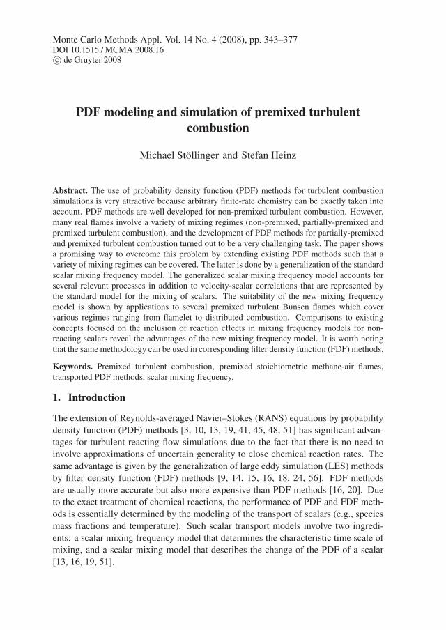
Monte Carlo Methods Appl. Vol. 14 No. 4 (2008), pp. 343–377DOI 10.1515 / MCMA.2008.16c© de Gruyter 2008

PDF modeling and simulation of premixed turbulent

combustion

Michael Stöllinger and Stefan Heinz

Abstract. The use of probability density function (PDF) methods for turbulent combustion

simulations is very attractive because arbitrary finite-rate chemistry can be exactly taken into

account. PDF methods are well developed for non-premixed turbulent combustion. However,

many real flames involve a variety of mixing regimes (non-premixed, partially-premixed and

premixed turbulent combustion), and the development of PDF methods for partially-premixed

and premixed turbulent combustion turned out to be a very challenging task. The paper shows

a promising way to overcome this problem by extending existing PDF methods such that a

variety of mixing regimes can be covered. The latter is done by a generalization of the standard

scalar mixing frequency model. The generalized scalar mixing frequency model accounts for

several relevant processes in addition to velocity-scalar correlations that are represented by

the standard model for the mixing of scalars. The suitability of the new mixing frequency

model is shown by applications to several premixed turbulent Bunsen flames which cover

various regimes ranging from flamelet to distributed combustion. Comparisons to existing

concepts focused on the inclusion of reaction effects in mixing frequency models for non-

reacting scalars reveal the advantages of the new mixing frequency model. It is worth noting

that the same methodology can be used in corresponding filter density function (FDF) methods.

Keywords. Premixed turbulent combustion, premixed stoichiometric methane-air flames,

transported PDF methods, scalar mixing frequency.

1. Introduction

The extension of Reynolds-averaged Navier–Stokes (RANS) equations by probability

density function (PDF) methods [3, 10, 13, 19, 41, 45, 48, 51] has significant advan-

tages for turbulent reacting flow simulations due to the fact that there is no need to

involve approximations of uncertain generality to close chemical reaction rates. The

same advantage is given by the generalization of large eddy simulation (LES) methods

by filter density function (FDF) methods [9, 14, 15, 16, 18, 24, 56]. FDF methods

are usually more accurate but also more expensive than PDF methods [16, 20]. Due

to the exact treatment of chemical reactions, the performance of PDF and FDF meth-

ods is essentially determined by the modeling of the transport of scalars (e.g., species

mass fractions and temperature). Such scalar transport models involve two ingredi-

ents: a scalar mixing frequency model that determines the characteristic time scale of

mixing, and a scalar mixing model that describes the change of the PDF of a scalar

[13, 16, 19, 51].

344 Michael Stöllinger and Stefan Heinz

Most of the previous applications of PDF and FDF methods were related to simu-

lations of non-premixed turbulent combustion. In this case, the characteristic length

and time scales of scalar fields are usually larger than the characteristic length and

time scales of turbulent motions. Correspondingly, the scalar mixing frequency can

be assumed to be controlled by the frequency of large-scale turbulent motions. The

performance of scalar mixing models for non-premixed turbulent combustion is rela-

tively well investigated [13, 17, 36, 37, 59]. Mitarai et al. [37] compared predictions

of different mixing models to the results of direct numerical simulation (DNS). Merci

et al. [32, 33, 34, 35] and Xu and Pope [62] studied various scalar mixing models in

turbulent natural gas diffusion flames. The FDF method also has been successfully

applied to non-premixed flames by Raman et al. [53] and Sheiki et al. [55].

Applications of PDF and FDF methods to premixed turbulent combustion are more

complicated than calculations of non-premixed turbulent combustion. The appearance

of fast flamelet chemistry may result in very thin reaction zones such that scalar mixing

can take place on scales which are much smaller than all scales of turbulent motions

[2, 29, 39, 49]. Correspondingly, there exist only a few applications of PDF methods

to premixed flames. To overcome problems of earlier approaches, Mura et al. [39]

recently suggested a PDF model where the outer parts of the flame structure (reac-

tant side and product side) are described by a standard scalar mixing model whereas

the inner part (the reaction zone) is described by a flamelet model. However, this ap-

proach is complicated and related to several questions (e.g. regarding the matching

of both combustion regimes). The scalar mixing frequency is provided via a transport

equation for the scalar dissipation rate which involves effects of chemical reactions

in corresponding equations for non-reacting scalars. The model of Mura et al. [39]

requires the adjustment of six parameters to the flow considered, the modeling of the

dissipation rate of non-reacting scalars does not agree with many other models [54],

and there are questions regarding the inclusion of chemical reaction effects (see Sec-

tion 7). More recently, Lindstedt and Vaos [29] and Cha and Trouillet [6, 7] developed

models that relate the scalar mixing frequency of reacting scalars to the characteris-

tic frequency of turbulent motions and the scalar mixing frequency of non-reacting

scalars, respectively. Both approaches use flamelet ideas in conjunction with several

other assumptions: e.g., the assumption of a local equilibrium between production and

dissipation in the scalar dissipation rate equation [29], and the assumption of local

homogeneity and isotropy [6, 7]). The investigations reported here reveal that these

assumptions are not satisfied in general.

The paper will address the questions described in the preceding paragraph in the

following way. Section 2 deals with a description of the PDF modeling approach. The

modeling of molecular scalar mixing is the concern of Section 3. The problems related

to the use of the standard model for scalar mixing will be described, and a generaliza-

tion of the standard mixing frequency model will be presented. The following sections

describe applications of the generalized mixing frequency model to simulations of

PDF modeling of premixed turbulent combustion 345

three premixed turbulent Bunsen flames which cover various regimes ranging from

flamelet to distributed combustion. The flames considered are discussed in Section 4,

and the flame simulations are described in Section 5. Section 6 presents simulation

results obtained with the scalar mixing frequency model introduced in Section 3 in

comparison to measurements. Comparisons with modeling approaches applied previ-

ously will be discussed in Section 7. Section 8 deals with conclusions of this work.

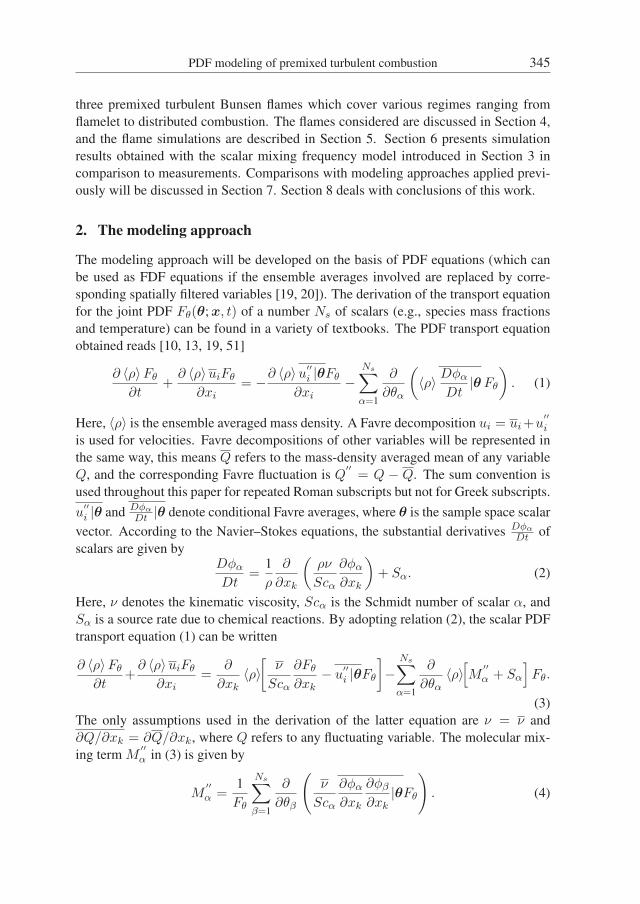
2. The modeling approach

The modeling approach will be developed on the basis of PDF equations (which can

be used as FDF equations if the ensemble averages involved are replaced by corre-

sponding spatially filtered variables [19, 20]). The derivation of the transport equation

for the joint PDF Fθ(θ; x, t) of a number Ns of scalars (e.g., species mass fractions

and temperature) can be found in a variety of textbooks. The PDF transport equation

obtained reads [10, 13, 19, 51]

∂ 〈ρ〉Fθ

∂t+

∂ 〈ρ〉uiFθ

∂xi= −∂ 〈ρ〉u

′′

i |θFθ

∂xi−

Ns∑

α=1

∂

∂θα

(

〈ρ〉 Dφα

Dt|θ Fθ

)

. (1)

Here, 〈ρ〉 is the ensemble averaged mass density. A Favre decomposition ui = ui +u′′

i

is used for velocities. Favre decompositions of other variables will be represented in

the same way, this means Q refers to the mass-density averaged mean of any variable

Q, and the corresponding Favre fluctuation is Q′′

= Q − Q. The sum convention is

used throughout this paper for repeated Roman subscripts but not for Greek subscripts.

u′′

i |θ and Dφα

Dt |θ denote conditional Favre averages, where θ is the sample space scalar

vector. According to the Navier–Stokes equations, the substantial derivatives Dφα

Dt of

scalars are given byDφα

Dt=

1

ρ

∂

∂xk

(

ρν

Scα

∂φα

∂xk

)

+ Sα. (2)

Here, ν denotes the kinematic viscosity, Scα is the Schmidt number of scalar α, and

Sα is a source rate due to chemical reactions. By adopting relation (2), the scalar PDF

transport equation (1) can be written

∂ 〈ρ〉Fθ

∂t+

∂ 〈ρ〉uiFθ

∂xi=

∂

∂xk〈ρ〉[

ν

Scα

∂Fθ

∂xk− u

′′

i |θFθ

]

−Ns∑

α=1

∂

∂θα〈ρ〉[

M′′

α + Sα

]

Fθ.

(3)

The only assumptions used in the derivation of the latter equation are ν = ν and

∂Q/∂xk = ∂Q/∂xk, where Q refers to any fluctuating variable. The molecular mix-

ing term M′′

α in (3) is given by

M′′

α =1

Fθ

Ns∑

β=1

∂

∂θβ

(

ν

Scα

∂φα

∂xk

∂φβ

∂xk|θFθ

)

. (4)

346 Michael Stöllinger and Stefan Heinz

M′′

α is written as a Favre fluctuation because expression (4) reveals that the mean of

M′′

α disappears,

M ′′

α = 0. (5)

By multiplying equation (3) with the corresponding variables and integrating over the

scalar sample space, one finds for scalar means φα and scalar variances φ′′2α the trans-

port equations

Dφα

Dt=

1

〈ρ〉∂

∂xk〈ρ〉(

ν

Scα

∂φα

∂xk− u

′′

kφ′′

α

)

+ Sα, (6)

and

Dφ′′2α

Dt=

1

〈ρ〉∂

∂xk〈ρ〉(

ν

Scα

∂φ′′2α

∂xk− u

′′

kφ′′2α

)

− 2u′′

kφ′′

α

∂φα

∂xk− 2εα + 2S′′

αφ′′

α. (7)

Here, D/Dt = ∂/∂t + uk ∂/∂xk refers to the mean Lagrangian time derivative, and

the scalar dissipation rate εα is given by

εα =ν

Scα

∂φ′′

α

∂xk

∂φ′′

α

∂xk. (8)

The definition (4) of M′′

α determines a relationship between the molecular mixing term

M′′

α and scalar dissipation rate εα,

M ′′

αφ′′

α = −εα − ν

Scα

∂φα

∂xk

∂φα

∂xk. (9)

By replacing εα in the scalar variance equation (7) according to relation (9) one obtains

a relation between M ′′

αφ′′

α and the transport of scalar variances which will be used

below for the modeling of M′′

α .

The approach applied implies the need to parametrize the conditional turbulent

scalar flux u′′

i |θ. This flux will be modeled by the usual gradient diffusion assumption

[10, 13, 19, 51],

u′′

i |θ Fθ = − νt

Sct

∂Fθ

∂xi. (10)

Here, Sct refers to a constant turbulent Schmidt number and νt = Cµkτ denotes the

turbulent viscosity: k is the turbulent kinetic energy, τ is the dissipation time scale of

turbulence, and Cµ is a dimensionless parameter. Expression (10) for the conditional

turbulent scalar flux implies the usual gradient-diffusion models for the turbulent scalar

flux and turbulent scalar variance flux,

u′′

i φ′′

α = − νt

Sct

∂φα

∂xi, u

′′

i φ′′2α = − νt

Sct

∂φ′′2α

∂xi. (11)

PDF modeling of premixed turbulent combustion 347

For simplicity, we will assume that Scα = Sct. The resulting transport equation for

the scalar PDF is then given by

∂ 〈ρ〉Fθ

∂t+

∂ 〈ρ〉ui Fθ

∂xi=

∂

∂xi〈ρ〉 ν + νt

Sct

∂Fθ

∂xi−

Ns∑

α=1

∂

∂θα〈ρ〉(

M′′

α + Sα

)

Fθ. (12)

Equation (12) implies for scalar means the equation

Dφα

Dt=

1

〈ρ〉∂

∂xk〈ρ〉(

ν + νt

Sct

∂φα

∂xk

)

+ Sα. (13)

By adopting relation (9) for εα, the scalar variance equation implied by equation (12)

reads

Dφ′′2α

Dt=

1

〈ρ〉∂

∂xk

(

〈ρ〉 ν + νt

Sct

∂φ′′2α

∂xk

)

+ 2ν + νt

Sct

∂φα

∂xk

∂φα

∂xk+ 2M ′′

αφ′′

α + 2S′′

αφ′′

α. (14)

3. Molecular mixing modeling

The scalar PDF transport equation (12) is unclosed as long as the molecular mixing

term M′′

α is not specified. The latter can be done in a variety of ways [10, 13, 19, 51].

We will use a parametrization of M′′

α according to the interaction-by-exchange-with-

the-mean (IEM) mixing model [11, 61],

M′′

α = −Cα

2τφ

′′

α. (15)

The model (15) represents the standard mixing model which is used in most simu-

lations of turbulent reacting flows [13, 51]. The reason for that is given by the sim-

plicity of the model (15). The model (15) contains two ingredients: a scalar mixing

model that describes changes of scalar values, and a scalar mixing frequency model

that determines the characteristic time scale of mixing. The scalar mixing is modeled

by −φ′′

α, which corresponds to the idea that scalar fluctuations φ′′

α tend to disappear

(scalar values φα tend to relax to their mean value φα). The scalar mixing frequency

ωα = Cα/(2τ) is modeled in proportionality to the mixing frequency 1/τ of large-

scale turbulent motions, where Cα is a nondimensional parameter. The consideration

of the relatively simple standard mixing model (15) represents a natural first step of

investigations of the performance of improved models for the mixing frequency ωα in

M′′

α models [21]. Justification for this approach arises from the observation that the

problem considered requires, first of all, an improved modeling of the scalar mixing

frequency ωα = Cα/(2τ) (see the discussion in the introduction). The question of

whether the use of other scalar mixing models may further improve simulation results

will be the concern of future efforts.

348 Michael Stöllinger and Stefan Heinz

Expression (15) requires the definition of Cα in order to specify the scalar mixing

frequency ωα = Cα/(2τ). The scalar mixing frequency ωα determines, first of all, the

evolution of the scalar variance. Thus, the equation for scalar variances represents the

natural basis for the definition of Cα. By adopting expression (15) in equation (14),

the scalar variance equation can be written

eα = Pα − CαBα. (16)

Here, Bα is given by Bα = φ′′2α /τ , and eα and Pα are given by the expressions

eα =Dφ′′2

α

Dt− 1

〈ρ〉∂

∂xk

(

〈ρ〉 ν + νt

Sct

∂φ′′2α

∂xk

)

− 2S′′

αφ′′

α, (17)

Pα = 2ν + νt

Sct

∂φα

∂xk

∂φα

∂xk. (18)

Equation (16) can be used to find an appropriate constant value for Cα on the basis

of DNS data. The latter can be done, for example, by adopting Overholt and Pope’s

DNS data of passive scalar mixing in homogeneous isotropic stationary turbulence

with imposed constant mean scalar gradient [42]. For the flow considered one finds

that eα = 0, this means there is a local equilibrium between the production Pα and dis-

sipation CαBα of scalar variances, Pα = CαBα. Overholt and Pope’s DNS data then

provide Cα = (1.8; 2.1; 2.2) for Taylor-scale Reynolds numbers Reλ = (28; 52; 84),respectively (these Cα values were obtained without using the gradient-diffusion ap-

proximation (11) for the turbulent scalar flux). An analysis of the Reynolds number

dependence of Cα indicates a value Cα = 2.5 for infinitely high Taylor-scale Reynolds

numbers [19]. Based on these findings, the standard model for Cα is given by the use

of a constant value Cα ≈ 2 for Cα [13, 19, 51]. However, a constant value of Cα

means that the turbulent velocity and scalar fields are strongly correlated such that the

scalar mixing frequency ωα = Cα/(2τ) is completely controlled by the frequency 1/τof large-scale turbulent motions. There is, however, no guarantee that a constant value

for Cα represents a reasonable approximation for flows which are more complex than

homogeneous isotropic and stationary turbulence. For example, the use of a constant

value for Cα appears to be inappropriate if the characteristic time and length scales

of scalar fields are found below the corresponding scales of turbulent motions, which

is a characteristic feature of premixed turbulent combustion. Correspondingly, several

attempts have been made to overcome the limitations of using a constant value for Cα

[27, 29, 38]. Unfortunately, all these approaches presented previously are faced with

significant problems: see the detailed discussion provided in Section 7. To overcome

the problems related to the use of a constant value for Cα, an attempt to generalize the

standard model for Cα will be made in the following.

PDF modeling of premixed turbulent combustion 349

The basic idea of the approach applied is the following one. In extension of the

standard model for Cα one may assume that eα is small compared to Pα and CαBα

in (16), this means one assumes that relation (16) can be basically characterized by

a local equilibrium between the production Pα and dissipation CαBα of scalar vari-

ances. Such an approach is often used, for example, for the derivation of algebraic

stress models [13, 19, 51]. In other words, eα may be seen as a relatively small de-

viation from a local equilibrium between Pα and CαBα. On this basis, Cα can be

calculated by the constraint to minimize the deviation eα from the local equilibrium.

What is the most convenient way to formulate such a constraint for the calculation

of Cα? Cα depends on eα, Pα, and Bα according to relation (16). The calculation

of eα, Pα, and Bα in terms of simulation results will be affected by numerical errors

due to the discretization of equations and the finite number of particles involved in the

Monte Carlo simulation. Thus, eα, Pα, and Bα calculated in this way represent fluctu-

ating variables. The most convenient way to calculate Cα under these conditions is to

minimize the averaged squared deviations⟨

e2α

⟩

Tfrom the local equilibrium between

production and dissipation of scalar variances (see the detailed explanations below).

Here, 〈Q〉T refers to a temporal average of any variable Q. This idea of calculating

Cα has some similarity with the calculation of the dynamic Smagorinsky coefficient

in LES [51]. However, there is a problem related to this approach. The production Pα

results from the modeling of velocity-scalar correlations u′′

kφ′′

α: see equations (7) and

(11). Thus, the assumption of minimal deviations from a local equilibrium between

the production and dissipation of scalar variances means that the mixing of scalars is

controlled by the turbulent velocity field. This condition cannot be considered to be

satisfied for premixed combustion where the characteristic mixing time scale may well

be smaller than the characteristic time scales of the velocity field. Indeed, the applica-

tion of this approach to the flame simulations described below leads to poor results for

the F3 and F2 flames as compared to measurements, and it leads to a global extinction

of the F1 flame in simulations.

Thus, the idea discussed in the preceding paragraph will be modified by consider-

ing a generalized local equilibrium between the production and dissipation of scalar

variances. The term 2S′′

αφ′′

α due to chemical reactions accounts for a correlation be-

tween scalar mixing and chemical reactions which may well be relevant in addition

to velocity-scalar correlations. Therefore, the term 2S′′

αφ′′

α will be added to the rele-

vant terms Pα and CαBα on the right-hand side of (16). To evaluate the relevance of

the second term on the left-hand side of (16), it is helpful to split this term into two

contributions,

1

〈ρ〉∂

∂xk

(

〈ρ〉 ν + νt

Sct

∂φ′′2α

∂xk

)

=ν + νt

Sct

∂2φ′′2α

∂x2k

+1

〈ρ〉Sct

∂ 〈ρ〉 (ν + νt)

∂xk

∂φ′′2α

∂xk. (19)

The first contribution on the right-hand side of (19) can be combined with the pro-

duction Pα on the right-hand side of (16). However, the relevance of the last term in

350 Michael Stöllinger and Stefan Heinz

(19) seems to be low because there is no reason to expect a systematic effect on the

turbulent mixing of scalars. Indeed, the simulation results reported below show that

the modification of the first term on the right-hand side of (19) due to the last term is

less than 5%. Thus, the last term of (19) will be added to the terms of minor relevance

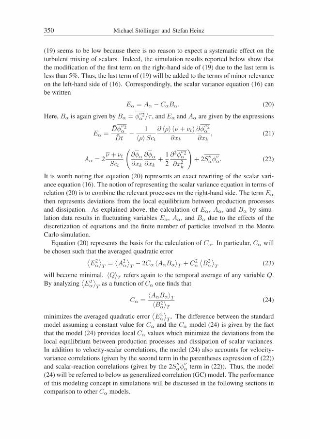
on the left-hand side of (16). Correspondingly, the scalar variance equation (16) can

be written

Eα = Aα − CαBα. (20)

Here, Bα is again given by Bα = φ′′2α /τ , and Eα and Aα are given by the expressions

Eα =Dφ′′2

α

Dt− 1

〈ρ〉Sct

∂ 〈ρ〉 (ν + νt)

∂xk

∂φ′′2α

∂xk, (21)

Aα = 2ν + νt

Sct

(

∂φα

∂xk

∂φα

∂xk+

1

2

∂2φ′′2α

∂x2k

)

+ 2S′′

αφ′′

α. (22)

It is worth noting that equation (20) represents an exact rewriting of the scalar vari-

ance equation (16). The notion of representing the scalar variance equation in terms of

relation (20) is to combine the relevant processes on the right-hand side. The term Eα

then represents deviations from the local equilibrium between production processes

and dissipation. As explained above, the calculation of Eα, Aα, and Bα by simu-

lation data results in fluctuating variables Eα, Aα, and Bα due to the effects of the

discretization of equations and the finite number of particles involved in the Monte

Carlo simulation.

Equation (20) represents the basis for the calculation of Cα. In particular, Cα will

be chosen such that the averaged quadratic error⟨

E2α

⟩

T=⟨

A2α

⟩

T− 2Cα 〈AαBα〉T + C2

α

⟨

B2α

⟩

T(23)

will become minimal. 〈Q〉T refers again to the temporal average of any variable Q.

By analyzing⟨

E2α

⟩

Tas a function of Cα one finds that

Cα =〈AαBα〉T〈B2

α〉T(24)

minimizes the averaged quadratic error⟨

E2α

⟩

T. The difference between the standard

model assuming a constant value for Cα and the Cα model (24) is given by the fact

that the model (24) provides local Cα values which minimize the deviations from the

local equilibrium between production processes and dissipation of scalar variances.

In addition to velocity-scalar correlations, the model (24) also accounts for velocity-

variance correlations (given by the second term in the parentheses expression of (22))

and scalar-reaction correlations (given by the 2S′′

αφ′′

α term in (22)). Thus, the model

(24) will be referred to below as generalized correlation (GC) model. The performance

of this modeling concept in simulations will be discussed in the following sections in

comparison to other Cα models.

PDF modeling of premixed turbulent combustion 351

4. The flames considered

The turbulent premixed F3, F2, and F1 flames studied experimentally by Chen et al.

[8] are considered to investigate the performance of the PDF modeling approach de-

scribed in Sections 2 and 3. The three highly stretched stoichiometric methane-air

flames cover a range of Reynolds and Damköhler numbers. Based on an order of mag-

nitude analysis Chen et al. [8] found that all three flames are located in the distributed

reaction zones regime [44]. In particular, the F1 flame is located at the borderline to the

well stirred reactor regime, and the F3 flame is located at the borderline to the flamelet

regime. This wide range of combustion conditions is often found in spark ignition

engines [1] which present one of the most important applications involving premixed

turbulent combustion. Due to the simple configuration, the broad range of combustion

conditions, and the high quality experimental database [8], the three flames consid-

ered are well appropriate to investigate the performance of PDF methods for premixed

turbulent combustion.

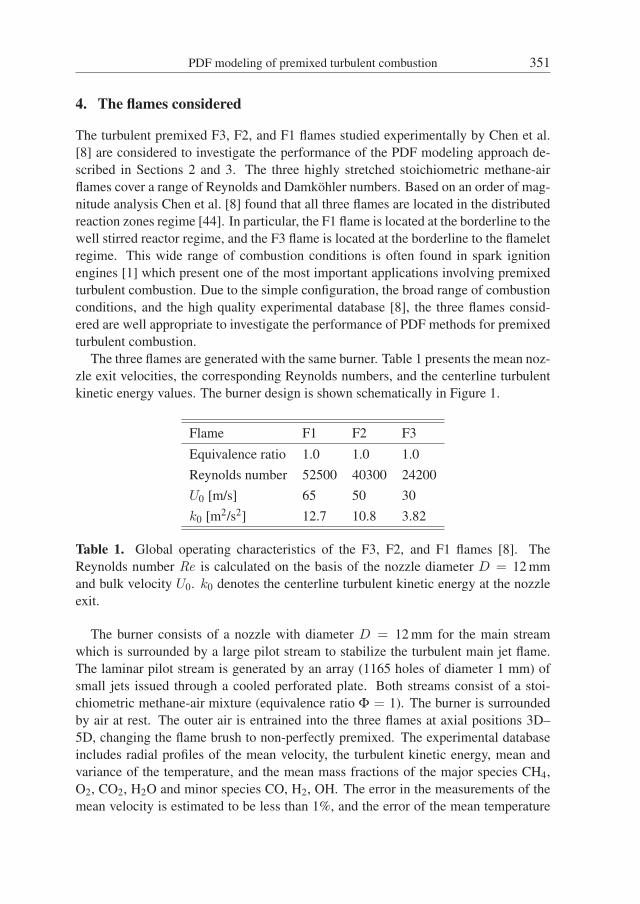
The three flames are generated with the same burner. Table 1 presents the mean noz-

zle exit velocities, the corresponding Reynolds numbers, and the centerline turbulent

kinetic energy values. The burner design is shown schematically in Figure 1.

Flame F1 F2 F3

Equivalence ratio 1.0 1.0 1.0

Reynolds number 52500 40300 24200

U0 [m/s] 65 50 30

k0 [m2/s2] 12.7 10.8 3.82

Table 1. Global operating characteristics of the F3, F2, and F1 flames [8]. The

Reynolds number Re is calculated on the basis of the nozzle diameter D = 12 mm

and bulk velocity U0. k0 denotes the centerline turbulent kinetic energy at the nozzle

exit.

The burner consists of a nozzle with diameter D = 12 mm for the main stream

which is surrounded by a large pilot stream to stabilize the turbulent main jet flame.

The laminar pilot stream is generated by an array (1165 holes of diameter 1 mm) of

small jets issued through a cooled perforated plate. Both streams consist of a stoi-

chiometric methane-air mixture (equivalence ratio Φ = 1). The burner is surrounded

by air at rest. The outer air is entrained into the three flames at axial positions 3D–

5D, changing the flame brush to non-perfectly premixed. The experimental database

includes radial profiles of the mean velocity, the turbulent kinetic energy, mean and

variance of the temperature, and the mean mass fractions of the major species CH4,

O2, CO2, H2O and minor species CO, H2, OH. The error in the measurements of the

mean velocity is estimated to be less than 1%, and the error of the mean temperature

352 Michael Stöllinger and Stefan Heinz

Figure 1. The burner design.

is expected to be less than 10%. The error in the measurements of the major species is

between 8% to 15%, and the error regarding the minor species is within 20% to 25%.

The flames considered have been studied numerically by using different combustion

models. Prasad and Gore [52] solved RANS equations. The averaged reaction rate was

closed with a flame surface density model which is valid under flamelet conditions

[47]. Therefore, only the F3 flame has been investigated. Herrmann [22] investigated

all three flames using a modified level set approach [45] that accounts for the effects of

the instantaneous flame structure and the entrainment of cold ambient air. The model is

strictly valid only under flamelet conditions. Pitsch and De Lageneste [46] formulated

the level set concept for LES of premixed flames and performed a F3 flame simulation.

They reported issues regarding the strong influence of boundary conditions in their

LES. Concerns include the significant heat losses due to the cooled burner surface,

which are estimated to reach up to 20% in the pilot flame.

The PDF method was applied first by Mura et al. [39] to simulate the F3 and F2

flames. They showed that the IEM mixing model [11, 61] combined with the standard

model ωα = 1/τ for the scalar mixing frequency is inapplicable to the two premixed

flames close to the flamelet regime. The use of the standard model corresponds to the

idea that the scalar mixing frequency is controlled by the inertial range turbulent mo-

tions. This assumption is valid for distributed combustion, but in the flamelet regime

the mixing process is controlled by the laminar flame length scale. Mura et al. [39]

suggested a PDF model where the outer parts of the flame structure (reactant side

and product side) are described by a standard mixing model and the inner part (reac-

PDF modeling of premixed turbulent combustion 353

tion zone) by a flamelet model. The scalar mixing frequency is provided by means

of a transport equation for the scalar dissipation rate. The latter equation was ob-

tained under the assumption of infinitely high Reynolds number and flamelet combus-

tion conditions. More recently, Lindstedt and Vaos [29] applied the transported PDF

model approach to F1, F2, and F3 flame simulations. They demonstrated the applica-

bility of the transported PDF model approach to premixed turbulent combustion in the

flamelet regime under the condition that the modeling of the scalar mixing frequency is

modified. They closed the molecular mixing term by using the modified coalescence-

dispersion (CD) mixing model [23]. Comparisons of results obtained with different

constants Cα = 2, 4, 6, 8 and a scalar mixing frequency model depending on the ratio

of the laminar flame velocity to the Kolmogorov velocity were performed. The latter

model will be referred to as Lindstedt–Vaos (LV) model. By assuming 10% heat loss

for the pilot flame, a stably burning F1 flame was obtained by adopting a constant

Cα > 4. However, by assuming 20% heat loss for the pilot flame, flame extinction

occurred over a wide range of constant Cα values. The latter problem did not appear

by using the LV model, this means the LV model enabled stable F1 flame simulations

for the case of 20% heat loss. Although the results obtained by Lindstedt and Vaos

are encouraging, one has to see that the LV model involves flamelet ideas in conjunc-

tion with assumptions that are not satisfied in general (for example, the assumption of

a local equilibrium between production and dissipation in the scalar dissipation rate

equation). Thus, the generality of the closures applied remains to be established [29].

5. Flame simulations

A hybrid PDF-RANS approach was used to simulate the turbulent premixed flames

described in Section 4. RANS equations were used for the calculation of the velocity

field. The conservation of mass and momentum equations applied are given by [51]

∂ 〈ρ〉∂t

+∂ 〈ρ〉ui

∂xi= 0, (25)

D〈ρ〉ui

Dt= − ∂p

∂xi+

∂

∂xj

[

〈ρ〉 ν

(

∂ui

∂xj+

∂uj

∂xi− 2

3

∂uk

∂xkδij

)]

−∂ 〈ρ〉u

′′

i u′′

j

∂xj. (26)

The Reynolds stress required to close equation (26) is given by a linear stress model,

u′′

i u′′

j =2

3kδij − νt

(

∂ui

∂xj+

∂uj

∂xi− 2

3

∂uk

∂xkδij

)

. (27)

The turbulent viscosity νt is given by the usual parametrization

νt = Cµk2

ε. (28)

354 Michael Stöllinger and Stefan Heinz

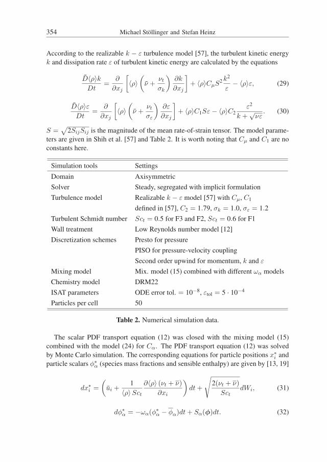
According to the realizable k − ε turbulence model [57], the turbulent kinetic energy

k and dissipation rate ε of turbulent kinetic energy are calculated by the equations

D〈ρ〉kDt

=∂

∂xj

[

〈ρ〉(

ν +νt

σk

)

∂k

∂xj

]

+ 〈ρ〉CµS2 k2

ε− 〈ρ〉ε, (29)

D〈ρ〉εDt

=∂

∂xj

[

〈ρ〉(

ν +νt

σε

)

∂ε

∂xj

]

+ 〈ρ〉C1Sε − 〈ρ〉C2

ε2

k +√

νε. (30)

S =√

2SijSij is the magnitude of the mean rate-of-strain tensor. The model parame-

ters are given in Shih et al. [57] and Table 2. It is worth noting that Cµ and C1 are no

constants here.

Simulation tools Settings

Domain Axisymmetric

Solver Steady, segregated with implicit formulation

Turbulence model Realizable k − ε model [57] with Cµ, C1

defined in [57], C2 = 1.79, σk = 1.0, σε = 1.2

Turbulent Schmidt number Sct = 0.5 for F3 and F2, Sct = 0.6 for F1

Wall treatment Low Reynolds number model [12]

Discretization schemes Presto for pressure

PISO for pressure-velocity coupling

Second order upwind for momentum, k and ε

Mixing model Mix. model (15) combined with different ωα models

Chemistry model DRM22

ISAT parameters ODE error tol. = 10−8, εtol = 5 · 10−4

Particles per cell 50

Table 2. Numerical simulation data.

The scalar PDF transport equation (12) was closed with the mixing model (15)

combined with the model (24) for Cα. The PDF transport equation (12) was solved

by Monte Carlo simulation. The corresponding equations for particle positions x∗i and

particle scalars φ∗α (species mass fractions and sensible enthalpy) are given by [13, 19]

dx∗i =

(

ui +1

〈ρ〉Sct

∂〈ρ〉 (νt + ν)

∂xi

)

dt +

√

2(νt + ν)

SctdWi, (31)

dφ∗α = −ωα(φ∗

α − φα)dt + Sα(φ)dt. (32)

PDF modeling of premixed turbulent combustion 355

Here, dWi denotes the increment of the ith component of a vectorial Wiener process.

The increments dWi are Gaussian random variables which are determined by their first

two moments,

〈dWi〉 = 0, 〈dWidWj〉 = δijdt. (33)

The scalar mixing frequency is defined by ωα = Cα/2τ . Cα is calculated according to

the GC model (24) for the fuel (CH4) mass fraction because combustion takes place

only if fuel is available. A numerical limit φ′′2α ≥ 10−6 was applied to avoid the

calculation of unphysically high values for Cα in regions where the scalar variance

φ′′2α becomes very small. Temporally averaged variables involved in the calculation of

Cα (24) were obtained by a moving average over 50 iterations. In this way, the solution

of the RANS equations (25)–(30) provides the mean velocity ui, turbulent viscosity νt

and turbulence time scale τ = k/ε. These variables are then used to solve the particle

equations (31)–(32). The mean density 〈ρ〉 and mean viscosity ν are calculated from

the particle compositions and temperatures and fed back into the RANS equations.

The steady-state RANS equations were discretized by the finite volume method.

Details can be found in Table 2. The particle equations (31)–(32) are solved numeri-

cally by a mid-point rule [4] in order to achieve second order accuracy in time. The

time step is determined from a local time stepping procedure [40]. Mean values of

scalar quantities are calculated by a weighted summation over particles in a cell. For

example, the term S′′

αφ′′

α was calculated by a summation∑Np

i=1 Sα(φ∗i)(φ∗iα −φα) over

all Np particles in a cell. The number of particles per cell is set to 50. A higher number

of particles per cell was found to have no effect on simulation results. The statistical

error is further reduced by averaging over the last 200 iterations [40]. All computations

presented have been performed by using the FLUENT code [12].

The chemical reaction rates Sα(φ) were provided by a skeletal chemical mechanism

DRM22 [26] consisting of 23 species (H2, H, O, O2, OH, H2O, HO2, H2O2, CH2,

CH2(S), CH3, CH4, CO, CO2, HCO, CH2O, CH3O, C2H2, C2H3, C2H4, C2H5, C2H6,

N2) and 104 elemental reaction. The suitability of the DRM22 mechanism will be

demonstrated in Section 6 by comparisons with results obtained with the full GRI-

2.11 mechanism [58]. The composition change due to chemical reactions was treated

by the in situ adaptive tabulation (ISAT) method developed by Pope [50].

The equations were solved on a 2-dimensional axisymmetric domain. The domain

extends up to 20D downstream (axial direction) from the nozzle exit plane and 6.5Din radial direction to allow entrainment of the ambient air. Here, D refers to the nozzle

diameter. The domain is discretized into 220 × 70 (axial by radial) cells. The grid is

non-uniform to improve the accuracy of computations in the flame region. The grid

independence of the solution has been checked by comparison with results obtained

on a 260 × 100 grid.

The boundary conditions applied are described in Table 3. The profiles for the

axial velocity and turbulent kinetic energy at the jet inlet have been taken from the

experimental database of Chen et al. [8]. The profile for the turbulent dissipation rate

356 Michael Stöllinger and Stefan Heinz

Stream Condition Values

Jet inlet Axial velocity U [m/s−1] Measured profiles [8]

k [m2s−2] Measured profiles [8]

ε [m2s−3] ε = (2k/3)3/2/llat; measured llat

T [K] 298

YCH40.0552

YO20.2201

Pilot flame Axial velocity U [m/s−1] 1.32

k [m2s−2] 10−3

ε [m2s−3] 0.1

T [K] 1785

YO25 · 10−4

YH2O 0.1236

YCO20.15

YCO 7.8 · 10−4

YH23 · 10−5

YOH 1.2 · 10−4

Rim Adiabatic wall

Air inlet Pressure inlet

Lateral boundary Pressure outlet

Outflow Pressure outlet

Table 3. Boundary conditions for the flame simulations.

has been calculated from the profile of the turbulent kinetic energy and measurements

of the lateral length scale llat by adopting the relation ε = (2k/3)3/2/llat [8]. The

pilot composition was calculated from the chemical equilibrium of a stoichiometric

methane-air mixture with 20% heat loss.

To reduce the computational time, the simulations were performed in two steps.

First, a laminar flame model [12] was used to generate realistic initial conditions for

PDF simulations. The PDF simulations were then initialized with the results from the

laminar flame model. Such a use of realistic initial conditions increases significantly

the convergence rate of PDF simulations. The computations have been performed

parallel on four 2.8GHz Opteron processors each equipped with 4GB of SDRAM. The

computational time required for a converged solution (involving approximately 30 000

iteration steps) was about 15 hours.

PDF modeling of premixed turbulent combustion 357

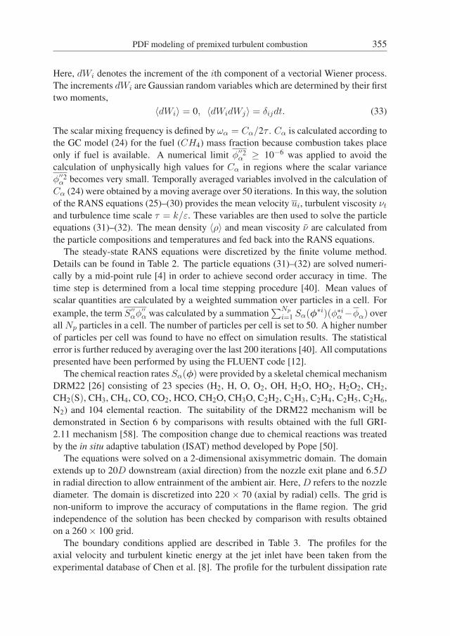
6. Simulation results

Radial profiles of the normalized mean axial velocity U/U0 are presented in Figure 2

at different axial positions h = x/D. The mean axial velocity U = u1 is normalized

by the bulk velocity U0 = 30, 50, 65 m/s for the F3, F2, and F1 flames, respectively.

The overall agreement between simulation results and measurements is excellent.

0 1 20

0.5

1

1.5

r / D

h=2.5

0 1 20

0.5

1

1.5h=4.5

0 1 20

0.5

1

1.5

U / U

0 h=6.5

0 1 20

0.5

1

1.5h=8.5

0 1 20

0.5

1

1.5Flame F3

h=10.5

0 1 20

0.5

1

1.5

r / D

0 1 20

0.5

1

1.50 1 2

0

0.5

1

1.50 1 2

0

0.5

1

1.50 1 2

0

0.5

1

1.5Flame F2

0 1 20

0.5

1

1.5

r / D

0 1 20

0.5

1

1.50 1 2

0

0.5

1

1.50 1 2

0

0.5

1

1.50 1 2

0

0.5

1

1.5Flame F1

Figure 2. Normalized mean axial velocities U/U0 for the F3, F2, and F1 flames. Dots

denote experimental results [8], and lines denote simulation results.

The thermal expansion within the turbulent jet can be recognized by the increase of

the axial velocity at radial positions r/D > 0.5 along the x-axis for all three flames.

As a result of this expansion, the shear layer (which is roughly located at the posi-

tion of the maximum gradient of the mean axial velocity) is pushed outward in radial

direction. This trend can also be seen in Figure 3 where radial profiles of the normal-

ized turbulent kinetic energy k/k0 (k0 = 3.82, 10.8, 12.7 m2/s2 for the F3, F2, and F1

flames, respectively) are shown. The peaks of the turbulent kinetic energy k are shifted

outward for increasing axial positions. The results for the higher Reynolds number F2

358 Michael Stöllinger and Stefan Heinz

0 1 20

5

10

15

r / D

h=2.5

0 1 20

5

10

15h=4.5

0 1 20

5

10

15

k / k

0 h=6.5

0 1 20

5

10

15h=8.5

0 1 20

5

10

15Flame F3

h=10.5

0 1 20

5

10

15

r / D

0 1 20

5

10

150 1 2

0

5

10

150 1 2

0

5

10

150 1 2

0

5

10

15Flame F2

0 1 20

5

10

15

r / D

0 1 20

5

10

150 1 2

0

5

10

150 1 2

0

5

10

150 1 2

0

5

10

15Flame F1

Figure 3. Normalized turbulent kinetic energy k/k0 for the F3, F2, and F1 flames.

Dots denote experimental results [8], and lines denote simulation results.

and F1 flames agree very well with the measurements whereas an overprediction of

the turbulent kinetic energy can be seen regarding the F3 flame, especially close to

the burner head. Similar overpredictions have been reported by Lindstedt and Vaos

[29]. The F3 flame was also studied by Pitsch and de Lageneste [46] by using LES

in combination with a level set approach. Their turbulent kinetic energy results show

a better agreement at h = 2.5 but a similar disagreement at h = 6.5. The F3 flame

has the lowest axial velocity and the highest temperature. Thus, low Reynolds number

effects which are not accounted for in the k − ε model applied may be the reason for

the turbulent kinetic energy overprediction. Radial profiles of the turbulence Reynolds

number Ret = kτ/ν are shown in Figure 4 at two axial positions for the three flames

considered.

Here, τ = k/ǫ is the characteristic time scale of large-scale turbulent motions, and

ν is the mean molecular viscosity. The results are shown in radial direction until the

flow becomes laminar. The profiles of Ret are qualitatively very similar for all three

flames since they are generated with the same burner.

PDF modeling of premixed turbulent combustion 359

0 1 20

500

1000

1500

2000

2500

h=2.5

r / D

Re

t

F1F2F3

0 1 20

500

1000

1500

h=8.5

r / D

Re

t

F1F2F3

Figure 4. Radial profiles of the turbulence Reynolds number Ret = kτ/ν for the

F1 (solid line), F2 (dashed line) and F3 (dashed-dotted line) flames at axial positions

h = 2.5 and h = 8.5.

Quantitatively, the turbulence Reynolds number of the F1 flame is about three times

larger than that of the F3 flame. For a cold round jet one would expect a peak of Ret

in the shear layer. Regarding the flames considered, the high temperature in the shear

layer drastically increases the molecular viscosity. The relatively high viscosity then

implies the monotonic decrease of Ret at h = 2.5 and the local minima observed in the

Ret profiles at h = 8.5. The appearance of small Ret values in the flame brush due to a

high viscosity (relaminization) is a well known phenomenon. These small Ret values

may explain the differences between simulation results and turbulent kinetic energy

measurements regarding the F3 flame: most turbulence models have been developed

under the assumption of high Ret values.

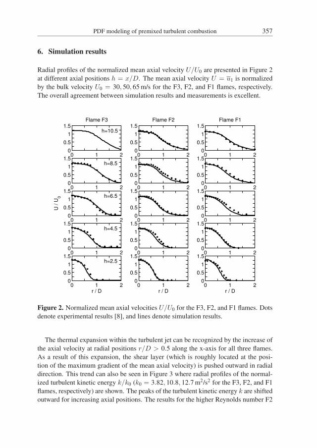
Figure 5 shows radial profiles of the mean reaction progress variable C = (T −Tu)/(Tb−Tu) [8] at different axial positions for the three flames considered. Here, T is

the mean temperature, Tb = 2248 K is the adiabatic flame temperature and Tu = 298 K

is the temperature of the surrounding air. The simulation results of the F3 flame agree

very well with the measurements. This agreement indicates that the new GC frequency

model is well applicable to flamelet conditions. The F2 and F1 flame simulation re-

sults show an overprediction of the progress variable at h = 2.5. Lindstedt and Vaos

[29] found a similar overprediction in their F1 flame simulations using the same pilot

inlet conditions. A reason for the observed overprediction of the temperature close to

the burner exit regarding the F2 and F1 flames could be given by the complex inter-

action between the turbulent jet and laminar pilot stream. Such flow conditions are

rather difficult to predict within the RANS framework. LES results for the F2 and F1

flames could clarify whether this is indeed the reason for the observed overprediction.

However, such LES results have not been reported so far. Possibly, a better agreement

between simulation results and measurements may be obtained by adopting refined

inlet conditions (e.g., a reduction of the pilot inlet temperature regarding the F2 and

F1 flames).

360 Michael Stöllinger and Stefan Heinz

0 1 20

0.5

1

r / D

h=2.5

0 1 20

0.5

1

h=4.5

0 1 20

0.5

1

C

h=6.5

0 1 20

0.5

1

h=8.5

0 1 20

0.5

1Flame F3

h=10.5

0 1 20

0.5

1

r / D

0 1 20

0.5

10 1 2

0

0.5

10 1 2

0

0.5

10 1 2

0

0.5

1Flame F2

0 1 20

0.5

1

r / D

0 1 20

0.5

10 1 2

0

0.5

10 1 2

0

0.5

10 1 2

0

0.5

1Flame F1

Figure 5. Mean reaction progress variable C for the F3, F2, and F1 flames. Dots

denote experimental results [8], and lines denote simulation results.

Figure 6 shows simulation results of the mean oxygen mass fraction YO2, and Figure

7 shows simulation results of the mean fuel (methane) mass fraction YCH4for the three

flames considered. Both oxygen and fuel concentrations are well predicted in all three

flames. The entrainment of surrounding air is clearly visible in Figure 6. It is most

intense in the highest Reynolds number F1 flame due to the high turbulence intensity.

Mean mass fractions of the product species YH2O and YCO2are shown in Figures 8 and

9, respectively. The H2O concentration results agree very well with the measurements

for all three flames. The CO2 concentration of the F3 flame is also well predicted

whereas the F2 and F1 flame results display a slight CO2 underprediction. Figure 10

presents radial profiles of the mean CO mass fraction YCO. This figure shows for all

three flames a significant overprediction of CO which increases downstream. This

finding could explain the underprediction of the CO2 concentration in the F2 and F1

flames: the slightly too high temperature levels in the F2 and F1 flame simulations

imply high CO levels and a corresponding slower oxidation of CO to CO2.

PDF modeling of premixed turbulent combustion 361

0 1 20

10

20 h=2.5

r / D

0 1 20

10

20 h=4.5

0 1 20

10

20 h=6.5

YO

2

[%

]

0 1 20

10

20 h=8.5

0 1 20

10

20 h=10.5

Flame F3

0 1 20

10

20

r / D

0 1 20

10

20

0 1 20

10

20

0 1 20

10

20

0 1 20

10

20

Flame F2

0 1 20

10

20

r / D

0 1 20

10

20

0 1 20

10

20

0 1 20

10

20

0 1 20

10

20

Flame F1

Figure 6. Mean O2 mass fraction YO2in percent for the F3, F2, and F1 flames. Dots

denote experimental results [8], and lines denote simulation results.

0 1 20

2

4

6h=2.5

r / D

0 1 20

2

4

6h=4.5

0 1 20

2

4

6h=6.5

YC

H4

[%

]

0 1 20

2

4

6h=8.5

0 1 20

2

4

6h=10.5

Flame F3

0 1 20

2

4

6

r / D

0 1 20

2

4

60 1 2

0

2

4

60 1 2

0

2

4

60 1 2

0

2

4

6Flame F2

0 1 20

2

4

6

r / D

0 1 20

2

4

60 1 2

0

2

4

60 1 2

0

2

4

60 1 2

0

2

4

6Flame F1

Figure 7. Mean CH4 mass fraction YCH4in percent for the F3, F2, and F1 flames. Dots

denote experimental results [8], and lines denote simulation results.

362 Michael Stöllinger and Stefan Heinz

0 1 20

10

20h=2.5

r / D

0 1 20

10

20h=4.5

0 1 20

10

20h=6.5

YH

2O

[%

]

0 1 20

10

20h=8.5

0 1 20

10

20h=10.5

Flame F3

0 1 20

10

20

r / D

0 1 20

10

200 1 2

0

10

200 1 2

0

10

200 1 2

0

10

20Flame F2

0 1 20

10

20

r / D

0 1 20

10

200 1 2

0

10

200 1 2

0

10

200 1 2

0

10

20Flame F1

Figure 8. Mean H2O mass fraction YH2O in percent for the F3, F2, and F1 flames.

Dots denote experimental results [8], and lines denote simulation results.

0 1 20

10

20h=2.5

r / D

0 1 20

10

20h=4.5

0 1 20

10

20h=6.5

YC

O2

[%

]

0 1 20

10

20h=8.5

0 1 20

10

20h=10.5

Flame F3

0 1 20

10

20

r / D

0 1 20

10

200 1 2

0

10

200 1 2

0

10

200 1 2

0

10

20Flame F2

0 1 20

10

20

r / D

0 1 20

10

200 1 2

0

10

200 1 2

0

10

200 1 2

0

10

20Flame F1

Figure 9. Mean CO2 mass fraction YCO2in percent for the F3, F2, and F1 flames. Dots

denote experimental results [8], and lines denote simulation results.

PDF modeling of premixed turbulent combustion 363

0 1 20

1

2

3h=2.5

r / D

0 1 20

1

2

3h=4.5

0 1 20

1

2

3h=6.5

YC

O [%

]

0 1 20

1

2

3h=8.5

0 1 20

1

2

3h=10.5

Flame F3

0 1 20

1

2

3

r / D

0 1 20

1

2

30 1 2

0

1

2

30 1 2

0

1

2

30 1 2

0

1

2

3Flame F2

0 1 20

1

2

3

r / D

0 1 20

1

2

30 1 2

0

1

2

30 1 2

0

1

2

30 1 2

0

1

2

3Flame F1

Figure 10. Mean CO mass fraction YCO in percent for the F3, F2, and F1 flames. Dots

denote experimental results [8], and lines denote simulation results.

The CO overestimation in the F3 flame cannot be explained in such a way since

the temperature and CO2 levels are well predicted. Similar high CO levels have been

reported by Lindstedt and Vaos [29]. The estimated error in the measurements of Chen

et al. [8] regarding the minor species CO and OH is between 20% and 25%. Thus,

the errors of measurements cannot explain the overpredictions of up to 100% which

are observed in the simulations. Simulations with the full GRI 2.11 mechanism [58]

do not improve the CO predictions (see the discussion of the influence of differently

complex chemical mechanisms in the following paragraph). Given the relatively well

predictions of all the other species it is unclear which reason may cause the observed

discrepancy between CO measurements and simulation results.

Figure 11 shows results of the mean OH mass fraction YOH. The OH levels are well

predicted for all the three flames for axial positions h ≤ 6.5. This finding is somewhat

unexpected regarding the F1 flame: its temperature is overpredicted for h ≤ 6.5,

and the OH-radical concentration is known to be very sensitive to temperature levels.

Moreover, all the measurements of OH seem to indicate a broader flame region, which

implies significant OH amounts in flame regions with very low mean temperatures.

Similar results have been found by Lindstedt and Vaos [29]. They concluded that

some caution may be required regarding the interpretation of the experimental data.

The influence of differently complex chemical mechanisms [5, 31] and finite-rate

chemistry effects [28] on the predictions of transported PDF methods have been stud-

ied in previous investigations. Two different chemical mechanisms have been applied

here to study the influence of the chemistry scheme: simulation results obtained with

364 Michael Stöllinger and Stefan Heinz

0 1 20

0.2

0.4 h=2.5

r / D

0 1 20

0.2

0.4 h=4.5

0 1 20

0.2

0.4 h=6.5

YO

H [%

]

0 1 20

0.2

0.4 h=8.5

0 1 20

0.2

0.4 h=10.5

Flame F3

0 1 20

0.2

0.4

r / D

0 1 20

0.2

0.4

0 1 20

0.2

0.4

0 1 20

0.2

0.4

0 1 20

0.2

0.4

Flame F2

0 1 20

0.2

0.4

r / D

0 1 20

0.2

0.4

0 1 20

0.2

0.4

0 1 20

0.2

0.4

0 1 20

0.2

0.4

Flame F1

Figure 11. Mean OH mass fraction YOH in percent for the F3, F2, and F1 flames. Dots

denote experimental results [8], and lines denote simulation results.

0 1 20

1

2

3

YC

O [

%]

r / D

h=4.5

0 1 20

1

2

3

YC

O [

%] h=8.5 gri2.11

drm22

0 1 20

0.2

0.4

YO

H [

%]

r / D

h=4.5

0 1 20

0.2

0.4

YO

H [

%]

h=8.5

Figure 12. Comparison of simulation results for the F3 flame obtained with the GRI

2.11 mechanism (solid line) and the skeletal DRM22 mechanism (dashed line). The

left column shows the CO mass fraction, and the right column shows the OH mass

fraction. In both simulations, the mixing model (15) was used in combination with the

GC model (24) for Cα.

PDF modeling of premixed turbulent combustion 365

the DRM22 [26] skeletal mechanism are compared in Figure 12 with results obtained

with the full GRI 2.11 mechanism [58]. CO and OH mass fractions of F3 flame simu-

lations are shown to address the overestimation of CO predictions and sensitivity of the

OH-radical concentration: see the discussion in the preceding paragraph. In both F3

flame simulations, the mixing model (15) was used in combination with the GC model

(24) for Cα. One observes that the results obtained with the different mechanisms are

almost identical. This fact indicates that the simplifications used to obtain the skeletal

mechanism DRM22 do not affect the simulation results.

7. Comparison with other scalar mixing frequency models

After demonstrating the good performance of the GC model in flame simulations, let

us compare the GC model with other ωα models for premixed turbulent combustion.

First, previously developed ωα models [6, 29, 38] will be described to explain the

underlying assumptions of these models. Second, flame calculations involving such

other ωα models will be compared to predictions based on the GC model.

An alternative approach to the direct derivation of models for the scalar mixing

frequency ωα is to consider a transport equation for the scalar dissipation rate εα. The

relation between εα and ωα provided by the expressions (9) and (15) is given by

ωαφ′′2α = εα +

ν

Scα

∂φα

∂xk

∂φα

∂xk. (34)

Usually, the relatively small last contribution in (34) is neglected in these approaches

(which corresponds to the assumption of high Reynolds numbers) such that ωα is given

by ωα = εα/φ′′2α . Transport equations for the scalar dissipation rate have been pro-

posed, for example, by Zeman and Lumley [63], Jones and Musonge [25], Mantel and

Borghi [30] and Mura and Borghi [38]. The structure of scalar dissipation rate models

[13, 54] can be illustrated by the model of Mura and Borghi [38], which is applicable

to premixed turbulent combustion. The latter model is given by

∂ 〈ρ〉 εMBα

∂t+

∂ 〈ρ〉 (uk − ULk)εMB

α

∂xk− ∂

∂xk

(

〈ρ〉Dt∂εMB

α

∂xk

)

(35)

=

(

cαε

k

P′

α

εMBα

+ cUε

k

P

ε+ α

ε

k− β

′ εMBα

φ′′2α

)

〈ρ〉εMBα .

The model (35) was derived on the basis of flamelet assumptions for infinitely high

Damköhler numbers. The source terms on the right-hand side are related to the produc-

tion and dissipation terms that appear in transport equations for the turbulent kinetic

energy and scalar variances. In particular, the production P by large-scale velocity

fields and the production P′

α by large-scale scalar fields are given by

P = νt∂uk

∂xk

∂uk

∂xk, P

′

α =νt

Sct

∂φα

∂xk

∂φα

∂xk. (36)

366 Michael Stöllinger and Stefan Heinz

The diffusion coefficient is given by Dt = νt/Scεα , where Scεα refers to the turbulent

Schmidt number in the εα equation. The propagation term ULkof flamelets and the

parameter β′

are given by

ULk=

SL

1 +√

2k/3/SL

∂φα

∂xk

(

∂φα

∂xj

∂φα

∂xj

)− 12

, β′

= β

(

1 − 2

3cεα

SL√k

)

. (37)

Here, SL is the laminar burning velocity of the mixture. The model constants are

given by α = 0.9, β = 4.2, cU = cα = 1.0, cεα = 0.1 and Scεα = 1.3 [60]. The

model (35) will be referred to below as Mura and Borghi (MB) model. It is worth

noting, however, that there are some questions related to the MB model. The reaction

contributions in the MB model are given by the flamelet propagation velocity ULkand

the term 2/3cεαSL/√

k in the expression for the β′

coefficient. To see the importance

of the flamelet propagation as compared to the fluid velocity we consider the ratio

Z =√

ULkULk

/√

ukuk between the magnitude of the flamelet propagation velocity

and the magnitude of the fluid velocity.

Figure 13 shows the values of the ratio Z and the term 2/3cεαSL/√

k along the

mean flame front position (see the definition below) for the F3 flame. The ratio Zremains less than 0.01 for most parts of the flame. Hence, the influence of the flamelet

propagation velocity is negligible. The factor 2/3cεαSL/√

k is less than 0.02, which

implies that β′ ≈ β. The two reactive contributions Z and 2/3cεαSL/√

k are even

smaller for the F2 and F1 flames (not shown) since the fluid velocity and the turbulence

levels are much higher in these flames. Thus, the MB model (35) reduces to a transport

equation for a passive scalar regarding the flames considered. The latter cannot be seen

to be justified since the fuel mass fraction (which was used for the calculation of the

scalar dissipation rate) is a highly reactive scalar. It is interesting to compare the MB

0 4 8 12 160

0.02

0.04

0.06

0.08

X / D

2/3cεS

L/k

1/2

Z

Figure 13. Reaction contributions 2/3cεαSL/√

k and Z =√

ULkULk

/√

ukuk in the

MB model (35) for the F3 flame along the mean flame front.

PDF modeling of premixed turbulent combustion 367

model for non-reacting scalars (this means for ULk= 0 and β

′

= β) with the model

of Jones and Musonge [25] and a variety of other scalar dissipation rate equations

studied by Sanders and Goekalb [54]. This comparison reveals a significant difference

between the MB model and other models for the scalar dissipation rate: the α ε/k term

acts as a production term in equation (35) whereas the corresponding term in the model

of Jones and Musonge [25] represents a sink term. Thus, the MB model disagrees with

many other models for the scalar dissipation rate of non-reacting scalars.

The underlying assumptions related to the algebraic scalar frequency model of Lind-

stedt and Vaos [29] can be seen by taking reference to the algebraic version of the MB

model. By assuming that the evolution of the scalar dissipation rate is dominated by

the source terms on the right-hand side, equation (35) implies an algebraic expression

for the scalar mixing frequency ωα = εα/φ′′2α ,

ωα =1

β(

1 − 23cεαSL/

√k)

(

cαP

′

α

εα+ cU

P

ε+ α

)

ε

k. (38)

The use of the first-order Taylor series approximation for the chemical reaction contri-

bution then results in

ωα =C

′

α

2

(

1 +2

3cεα

SL√k

)

ε

k, (39)

where C′

α = 2(cαP′

α/εα + cUP/ε + α)/β denotes a mixing parameter. Kuan et al.

[27] and Lindstedt and Vaos [29] derived an expression for ωα which is similar to

expression (39). Their scalar mixing frequency model is given by

ωLVα =

C′

α

2

(

1 + C∗α

ρu

〈ρ〉SL

vk

)

ε

k. (40)

Here, C′

α = 4 and C∗α = 1.2 are model constants [29]. ρu denotes the density of the

unburned mixture, 〈ρ〉 is the mean mass density, and vk is the Kolmogorov velocity.

The essential assumption related to the Lindstedt and Vaos (LV) model (40) is given

by the consideration of C′

α as a constant, which corresponds to the idea of velocity

and scalar fields that are characterized by a local equilibrium between production and

dissipation (P′

α/εα and P/ε are constant). This condition is not satisfied regarding the

flames considered here. Figure 14 shows radial profiles of the scalar production-to-

dissipation ratio P′

α/εα and the turbulence production-to-dissipation ratio P/ε in F3

flame simulations. As can be seen, the profiles of the production-to-dissipation ratios

vary significantly at both axial positions. Hence, the scalar production-to-dissipation

ratio P′

α/εα and the turbulence production-to-dissipation ratio P/ε are far from being

constants. Similar results have been found regarding the F2 and F1 flames (not shown).

It is also worth noting that the inclusion of the effect of chemical reactions differs from

expression (39), in particular, by the use of the Kolmogorov velocity vk instead of√

k.

368 Michael Stöllinger and Stefan Heinz

0 0.5 1 1.5 2.00

0.5

1.0

1.5

2.0

2.5

h=4.5

r / D

Pα

,/ε

α

P/ε

0 0.5 1 1.5 2.00

0.5

1.0

1.5

2.0

2.5

h=8.5

r / D

Pα

,/ε

α

P/ε

Figure 14. Radial profiles of the scalar production-to-dissipation ratio P′

α/εα (solid

line) and the turbulence production-to-dissipation ratio P/ε (dashed line) in F3 flame

simulations. The results have been obtained by adopting the GC model.

An alternative suggestion for the algebraic modeling of the scalar mixing frequency

was made by Cha and Trouillet [6]. Their model relies on the assumption that the large-

scale turbulent motions control the scalar mixing frequency (the mixing frequency of

reacting scalars is related to the mixing frequency of non-reacting scalars). However,

Cha and Trouillet’s model was developed for non-premixed turbulent flames. Thus, it

will be not considered for comparisons here.

The simplest ωα model is recovered by neglecting chemistry effects in the LV

model,

ωSTα =

Cα

2

ε

k. (41)

The model (41) will be referred to below as standard (ST-*) scalar mixing frequency

model, where * refers to the constant value of Cα applied. The basic assumption re-

lated to the model (41) is that the scalar mixing frequency ωα is controlled by the mix-

ing frequency ω = ε/k = 1/τ of large-scale turbulent motions. Let us have a closer

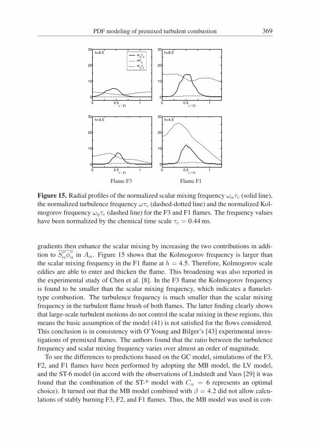
look at the validity of this assumption. Figure 15 shows radial profiles of the normal-

ized scalar mixing frequency ωατc, the normalized turbulence frequency ωτc, and the

normalized Kolmogorov frequency ωητc at axial positions h = 4.5 and h = 8.5 for the

F3 and F1 flames. Here, the Kolmogorov frequency ωη is defined by ωη = (ε/ν)1/2.

The frequency values have been normalized by the chemical time scale τc = 0.44 ms

which is defined as ratio of the laminar flame thickness and laminar burning velocity

[8]. High values of the normalized scalar mixing frequency are found within the tur-

bulent flame brush. The reason for that is given by the three terms involved in Aα (see

relation (22)). The correlation S′′

αφ′′

α between scalar mixing and chemical reactions

increases the scalar mixing frequency directly. The rapid consumption of the fuel in

the premixed flame steepens the gradients of the scalar mean and variance. The steep

PDF modeling of premixed turbulent combustion 369

0 0.5 1

0

10

20

30h=8.5

r / D

ωατc

ωτc

ωητc

0 0.5 1

0

10

20

30h=8.5

r / D

0 0.5 1

0

10

20

30h=4.5

r / D

Flame F3

0 0.5 1

0

10

20

30h=4.5

r / D

Flame F1

Figure 15. Radial profiles of the normalized scalar mixing frequency ωατc (solid line),

the normalized turbulence frequency ωτc (dashed-dotted line) and the normalized Kol-

mogorov frequency ωητc (dashed line) for the F3 and F1 flames. The frequency values

have been normalized by the chemical time scale τc = 0.44 ms.

gradients then enhance the scalar mixing by increasing the two contributions in addi-

tion to S′′

αφ′′

α in Aα. Figure 15 shows that the Kolmogorov frequency is larger than

the scalar mixing frequency in the F1 flame at h = 4.5. Therefore, Kolmogorov scale

eddies are able to enter and thicken the flame. This broadening was also reported in

the experimental study of Chen et al. [8]. In the F3 flame the Kolmogorov frequency

is found to be smaller than the scalar mixing frequency, which indicates a flamelet-

type combustion. The turbulence frequency is much smaller than the scalar mixing

frequency in the turbulent flame brush of both flames. The latter finding clearly shows

that large-scale turbulent motions do not control the scalar mixing in these regions, this

means the basic assumption of the model (41) is not satisfied for the flows considered.

This conclusion is in consistency with O’Young and Bilger’s [43] experimental inves-

tigations of premixed flames. The authors found that the ratio between the turbulence

frequency and scalar mixing frequency varies over almost an order of magnitude.

To see the differences to predictions based on the GC model, simulations of the F3,

F2, and F1 flames have been performed by adopting the MB model, the LV model,

and the ST-6 model (in accord with the observations of Lindstedt and Vaos [29] it was

found that the combination of the ST-* model with Cα = 6 represents an optimal

choice). It turned out that the MB model combined with β = 4.2 did not allow calcu-

lations of stably burning F3, F2, and F1 flames. Thus, the MB model was used in con-

370 Michael Stöllinger and Stefan Heinz

0 0.5 10

5

10

15

20

r / D

X /

D

F3

0 0.5 10

5

10

15

20

r / D

X /

D

F2

0 0.5 10

5

10

15

20

r / D

X /

D

F1

Figure 16. Position of the mean turbulent flame front obtained in F3, F2, and F1 flame

simulations by different scalar mixing frequency models: GC model (solid line), MB

model (dotted line), LV model (dashed line), ST-6 model (dashed-dotted line). Dots

denote experimental results. The circles denote curve fit results to the measured values

[8]. The iso-line temperatures are T 1 = 1300 K for the F1 flame, T 2 = 1400 K for the

F2 flame, and T 3 = 1500 K for the F3 flame respectively.

junction with β = 0.3, which provided the best agreement between simulation results

and measurements. Results obtained with the different frequency models are compared

with experimental data in Figure 16. This figure shows the mean flame front position

which is defined as iso-line of the mean temperature. The iso-line temperatures are

T 1 = 1300 K for the F1 flame, T 2 = 1400 K for the F2 flame, and T 3 = 1500 K

for the F3 flame respectively. The mean flame front position predicted by the GC

frequency model agrees well with the measured positions for all three flames. Thus,

the GC frequency model provides very good predictions for a range of combustion

regimes. The use of the MB model, LV model and ST-6 model results in significant

overestimations of the axial position of the flame tip regarding the F3 and F2 flames.

PDF modeling of premixed turbulent combustion 371

In the flame tip, the turbulent burning velocity has to balance the high axial velocity

of the jet. Thus, predictions of the axial position of the flame tip are very sensitive

to an accurate prediction of the turbulent burning velocity. In the F3 and F2 flames,

which are close to the flamelet regime, one finds strong axial gradients of mean scalars

and scalar variances in the flame tip. These gradients increase the scalar mixing fre-

quency (i.e., the mixing efficiency), which leads to an increase of the turbulent burning

velocity. The GC frequency model includes the effects of the strong gradients of scalar

means and variances in the flame tip such that the GC model provides an accurate pre-

diction of the flame tip position. In contrast to that, the ST-6 model and the LV model

do not include any effects of mean scalar and scalar variance gradients on the scalar

mixing. These models underestimate, therefore, the turbulent burning velocity, which

explains the overestimation of the flame tip position. The overprediction of the flame

tip position observed in the MB model simulations probably results from the underes-

timation of the chemical reaction contributions (see the discussion above). Regarding

the mean flame front position in F1 flame simulations one finds (with the exception of

the ST-6 model) that the predictions of the different mixing frequency models agree

well with the measurements. The F1 flame is closer to the well-stirred combustion

regime such that the scalar gradients are not as strong as in the F3 and F2 flames. The

mixing enhancement is less intense, which explains the close agreement of results.

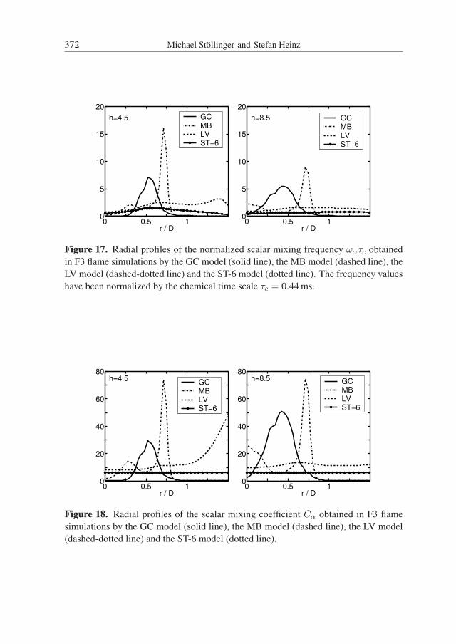
Figure 17 shows normalized mixing frequencies in F3 flame simulations according

to the four scalar frequency models considered. Figure 18 shows the corresponding

values of the mixing coefficient Cα. The GC model and the MB model display a peak

of the scalar mixing frequency. At both axial positions the peak predicted by the MB

model is located further outward than the peak predicted by the GC model. How can

this observation explain the different results for the mean flame front position? In an

analogy to a 1-d laminar flame the turbulent flame brush can be divided into a preheat

zone (fresh gas side of the flame front) and a reaction zone (burnt gas side of the flame

front). The peak value of the scalar mixing frequency predicted by the GC model is

then located in the preheat zone and the peak predicted by the MB model is located

in the reaction zone of the turbulent flame brush. The preheat zone is the zone where

the temperature of the fresh mixture is increased due to convection and diffusion of

heat from the reaction zone where most of the chemical reactions and the heat release

take place. High values of the scalar mixing frequency in the preheat zone allow for a

faster mixing of the temperature and thereby reactions can take place at further inward

radial locations. Without enhanced mixing in the preheat zone the location of the

reaction zone will be located further outward. Due to the heat release the location

of the reaction zone determines the mean flame front position. Therefore, one would

expect that the mean flame front position predicted by the GC model is located further

inward than the position predicted by the MB model. Exactly this feature can be seen

in Figure 16. The scalar mixing frequencies obtained with the ST-6 model and the

LV model differ significantly from the values predicted by the GC model and the MB

372 Michael Stöllinger and Stefan Heinz

0 0.5 10

5

10

15

20

h=4.5

r / D

GCMBLVST−6

0 0.5 10

5

10

15

20

h=8.5

r / D

GCMBLVST−6

Figure 17. Radial profiles of the normalized scalar mixing frequency ωατc obtained

in F3 flame simulations by the GC model (solid line), the MB model (dashed line), the

LV model (dashed-dotted line) and the ST-6 model (dotted line). The frequency values

have been normalized by the chemical time scale τc = 0.44 ms.

0 0.5 10

20

40

60

80h=4.5

r / D

GCMBLVST−6

0 0.5 10

20

40

60

80h=8.5

r / D

GCMBLVST−6

Figure 18. Radial profiles of the scalar mixing coefficient Cα obtained in F3 flame

simulations by the GC model (solid line), the MB model (dashed line), the LV model

(dashed-dotted line) and the ST-6 model (dotted line).

PDF modeling of premixed turbulent combustion 373

model: these scalar mixing frequency profiles are rather flat, and they do hardly show

a peak. The latter behavior results from the fact that both models do not account for

mean scalar and scalar variance gradients. As can be seen in Figure 18 the LV model

predicts unreasonably high values for the mixing parameter Cα in the outer part of the

flame at the position x/D = 4.5. This part of the flame corresponds to the burnt gas

side of a 1-d laminar flame which is dominated by convection of the hot gases. The

high values result from the reaction contribution in the LV model (40): small values

of the Kolmogorov velocity vk due to the high values of molecular viscosity and small

values of the mean density 〈ρ〉 (both are caused by the high temperature) result in high

values of the ratio ρu

〈ρ〉SL

vk.

8. Summary

Previously developed PDF methods for premixed turbulent combustion were consid-

ered in detail in Section 7. This discussion revealed significant problems of existing

approaches to model the scalar mixing frequency: the assumptions applied are not

justified in general (see the discussion related to the LV and ST-* models) or they are

in disagreement with other modeling efforts (see the discussion of the MB model).

The GC frequency model was introduced here as an alternative to these existing PDF

methods for premixed turbulent combustion. The modeling concept applied is rela-

tively general: the GC model is constructed such that deviations of a local equilibrium

between production processes and dissipation of scalar variances become minimal.

This concept offers significant conceptual advantages compared to existing methods.

Empirical parametrizations are not involved, there is no need to adjust several model

parameters to the flow considered, and effects of chemical reactions on scalar mixing

frequencies are involved without making assumptions that have an uncertain range of

applicability. It is also worth noting that the computational effort required to take ad-

vantage of the GC frequency model is reasonable. Compared to the LV model, for

example, the increase of computational costs is given by a factor of about 1.2.

The suitability of the GC scalar frequency model was demonstrated by applica-

tions to several turbulent premixed Bunsen flames that cover various regimes ranging

from flamelet to distributed combustion. Comparisons with existing scalar mixing fre-

quency models for premixed turbulent combustion revealed the advantages of the GC

frequency model. The main reason for these advantages is the following one. Existing

scalar mixing frequency models are constructed on the basis of the idea to implement

chemical reaction effects explicitly in equations for non-reacting scalars. However,

the studies reported here show that chemical reactions also have a significant implicit

effect on the scalar mixing frequency: a relatively small flame thickness due to the

fast chemistry implies significant gradients of scalar means and variances. The GC

frequency model relates the relatively small flame thickness to a relatively small scalar

mixing time scale (a relatively high scalar frequency) via the increase of gradients of

374 Michael Stöllinger and Stefan Heinz

scalar means and variances. This important effect is correctly represented in the GC

frequency model which explains its success.

Many real flames involve a variety of mixing regimes (non-premixed, partially-

premixed and premixed turbulent combustion). A significant advantage of the ap-

proach presented here is given by its applicability to such flames involving several

combustion regimes. Obviously, such applications will be very valuable for the further

evaluation of the capabilities of the approach presented. Questions that need further

investigations concern, for example, the relevance of using more complex scalar mix-

ing models and the relevance of using specific scalar mixing frequencies for different

species. It is worth noting that essentially the same scalar modeling approach can be

used to enable hybrid LES/FDF calculations.

Acknowledgments. This work has been supported by the German Research Foun-

dation (DFG) and Fluent Inc. (DFG Transfer Project 42). In particular, we are very

thankful to Dr. M. Braun (Fluent Germany) and Professor R. Friedrich for significant

support regarding the realization of this project. The authors gratefully acknowledge

valuable support of Dr. G. Goldin (Fluent USA) regarding the realization of computa-

tions. We are very thankful to Professor P. Jenny for many helpful comments on our

work. The computational resources have been provided by the Institute of Scientific

Computation (ISC) at the University of Wyoming.

References

1. J. Abraham, F. A. Williams and F. V. Bracco, A discussion of turbulent flame structure inpremixed charges, SAE Paper 850345 (1985).

2. M. S. Anand and S. B. Pope, Calculations of premixed turbulent flames by PDF methods,Combustion and Flame 67 (1987), pp. 127–142.

3. R. Borghi, Turbulent combustion modelling, Progress in Energy and Combustion Science14 (1988), pp. 245–292.

4. R. R. Cao and S. B. Pope, Numerical integration of stochastic differential equations: Weaksecond-order mid-point scheme for application in the composition PDF method, Journalof Computational Physics 185 (2003), pp. 194–212.

5. , The influence of chemical mechanisms on PDF calculations of nonpremixedpiloted jet flames, Combustion and Flame 143 (2005), pp. 450–470.

6. C. M. Cha and P. Trouillet, A model for the mixing time scale of a turbulent reactingscalar, Physics of Fluids 15 (2003), pp. 1375–1380.

7. , A subgrid-scale mixing model for large eddy simulations of turbulent reactingflows using the filtered density function, Physics of Fluids 15 (2003), pp. 1496–1504.

8. Y. C. Chen, N. Peters, G. A. Schneemann, N. Wruck, U. Renz and M. S. Mansour, Thedetailed flame structure of highly stretched turbulent premixed methane-air flames, Com-bustion and Flame 107 (1996), pp. 223–244.

9. P. J. Colucci, F. A. Jaberi, P. Givi and S. B. Pope, Filtered density function for large eddysimulation of turbulent reacting flows, Physics of Fluids 10 (1998), pp. 499–515.

PDF modeling of premixed turbulent combustion 375

10. C. Dopazo, Recent development in PDF methods, in: Turbulent Reacting Flows (P. A.Libby and F. A. Williams, eds.), pp. 375–474, Academic, New York, 1994.

11. C. Dopazo and E. E. O’Brien, An approach to autoignition of a turbulent mixture, ActaAstronautica 1 (1974), pp. 1239–1266.

12. FLUENT, 6.3 User Guide, FLUENT INC., Lebanon, NH, 2006.

13. R. O. Fox, Computational Models for Turbulent Reacting Flows, Cambridge UniversityPress, Cambridge, UK, 2003.

14. F. Gao and E. E. O’Brien, A large eddy simulation scheme for turbulent reacting flows,Physics of Fluids A5 (1993), pp. 1282–1284.

15. L. Y. M. Gicquel, P. Givi, F. A. Jaberi and S. B. Pope, Velocity filtered density functionfor large eddy simulation of turbulent flows, Physics of Fluids 14 (2002), pp. 1196–1213.

16. P. Givi, Filtered density function for subgrid scale modeling of turbulent combustion,AIAA Journal 44 (2006), pp. 16–23.

17. S. Heinz, On Fokker-Planck equations for turbulent reacting flows. Part 1. Probabilitydensity function for Reynolds-averaged Navier-Stokes equations, Flow, Turbulence andCombustion 70 (2003), pp. 115–152.

18. , On Fokker-Planck equations for turbulent reacting flows. Part 2. Filter densityfunction for large eddy simulation, Flow, Turbulence and Combustion 70 (2003), pp. 153–181.

19. , Statistical Mechanics of Turbulent Flows, Springer-Verlag, Berlin, 2003.

20. , Unified turbulence models for LES and RANS, FDF and PDF simulations, The-oretical and Computational Fluid Dynamics 21 (2007), pp. 99–118.

21. S. Heinz and D. Roekaerts, Reynolds number effects on mixing and reaction in a turbulentpipe flow, Chemical Engineering Science 56 (2001), pp. 3197–3210.

22. M. Herrmann, Numerical simulation of turbulent Bunsen flames with a level set flameletmodel, Combustion and Flame 145 (2006), pp. 357–375.

23. J. Janicka, W. Kolbe and W. Kollmann, Closure of the transport-equation for the pobabilitydensity function of turbulent scalar fields, Journal of Non-Equilibrium Thermodynamics 4(1979), pp. 47–66.

24. J. Janicka and A. Sadiki, Large eddy simulation of turbulent combustion systems, Pro-ceedings of the Combustion Institute 30 (2005), pp. 537–547.

25. W. P. Jones and P. Musonge, Closure of the Reynolds stress and scalar flux equations,Physics of Fluids 32 (1988), pp. 3589–3604.

26. A. Kazakov and M. Frenklach, DRM22, http://www.me.berkeley.edu/drm/.

27. T. S. Kuan, R. P. Lindstedt and E. M. Vaos, in: Advances in Confined Detonations andPulse Detonation Engines (G. Roy, ed.), pp. 17–40, Torus Press, Moscow, 2003, ISBN5-94588-012-4.

28. R. P. Lindstedt, S. A. Louloudi, J. J. Driscoll and V. Sick, Finite rate chemistry effects inturbulent reacting flows, Flow, Turbulence and Combustion 72 (2004), pp. 407–426.

29. R. P. Lindstedt and E. M. Vaos, Transported PDF modeling of high-Reynolds-numberpremixed turbulent flames, Combustion and Flame 145 (2006), pp. 495–511.

30. T. Mantel and R. Borghi, A new model of premixed wrinkeled flame propagation basedon a scalar dissipation equation, Combustion and Flame 96 (1994), pp. 443–457.

376 Michael Stöllinger and Stefan Heinz

31. A. R. Masri, R. Cao, S. B. Pope and G. M. Goldin, PDF calculations of turbulent liftedflames of H2/N2 fuel issuing into a vitiated co-flow, Combustion Theory and Modeling 8(2004), pp. 1–22.

32. B. Merci, B. Naud and D. Roekaerts, Flow and mixing fields for transported scalar PDFsimulations of a piloted jet diffusion flame ("Delft Flame III"), Flow, Turbulence andCombustion 74 (2005), pp. 239–272.

33. , Interaction between chemistry and micro-mixing modeling in transported PDFsimulations of turbulent non-premixed flames, Combustion Science and Technology 179(2006), pp. 153–172.

34. B. Merci, D. Roekaerts and B. Naud, Study of the performance of three micro-mixingmodels in transported scalar PDF simulations of a piloted jet diffusion flame ("Delft FlameIII"), Combustion and Flame 144 (2006), pp. 476–493.

35. B. Merci, D. Roekaerts, B. Naud and S. B. Pope, Study of the performance of differ-ent micro-mixing models in transported scalar PDF simulations of a piloted jet diffusionflame, Combustion and Flame 146 (2006), pp. 109–130.

36. D. W. Meyer and P. Jenny, A mixing model for turbulent flows based on parametrizedscalar profiles, Physics of Fluids 18 (2006), pp. 035105/1–15.

37. S. Mitarai, J. J. Riley and G. Kosály, Testing of mixing models for Monte Carlo probabilitydensity function simulations, Physics of Fluids 17 (2005), pp. 047101/1–15.

38. A. Mura and R. Borghi, Towards an extended scalar dissipation equation for turbulentpremixed combustion, Combustion and Flame 133 (2003), pp. 193–196.

39. A. Mura, F. Galzin and R. Borghi, A unified PDF-flamelet model for turbulent premixedcombustion, Combustion Science and Technology 175 (2003), pp. 1573–1609.

40. M. Muradoglu and S. B. Pope, Local time-stepping algorithm for solving the probabilitydensity function turbulence model equations, AIAA Journal 40 (2002), pp. 1755–1763.

41. E. E. O’Brien, The probability density function (PDF) approach to reacting turbulentflows, in: Turbulent Reacting Flows (P. A. Libby and F. A. Williams, eds.), pp. 185–218,Springer-Verlag, Berlin, 1980.

42. M. R. Overholt and S. B. Pope, Direct numerical simulation of a passive scalar with im-posed mean gradient in isotropic turbulence, Physics of Fluids 8 (1996), pp. 3128–3148.

43. F. O’Young and R. W. Bilger, Scalar gradient and related quantities in turbulent premixedflames, Combustion and Flame 109 (1997), pp. 682–700.

44. N. Peters, Laminar flamelet concepts in turbulent combustion, 21st Symposium (Int.) onCombustion, The Combustion Institute (1986), pp. 1231–1250, Pittsburgh.

45. , Turbulent Combustion, Cambridge University Press, Cambridge, UK, 2000.

46. H. Pitsch and L. D. De Lageneste, Large eddy simulation of premixed turbulent com-bustion using a level-set approach, Proceedings of the Combustion Institute 29 (2002),pp. 2001–2008.

47. T. P. Poinsot and D. Veynante, Theoretical and Numerical Combustion, Second ed, Ed-wards, Philadelphia, 2005.

48. S. B. Pope, PDF methods for turbulent reactive flows, Progress in Energy and CombustionScience 11 (1985), pp. 119–192.

49. , Turbulent premixed flames, Annual Review of Fluid Mechanics 19 (1987),pp. 237–270.

PDF modeling of premixed turbulent combustion 377

50. , Computationally efficient implementation of combustion chemistry using a insitu adaptive tabulation, Combustion Theory and Modelling 1 (1997), pp. 41–63.

51. , Turbulent Flows, Cambridge Univerity Press, Cambridge, UK, 2000.

52. R. O. S. Prasad and J. P. Gore, An evaluation of flame surface density models for turbulentpremixed jet flames, Combustion and Flame 116 (1998), pp. 1–14.

53. V. Raman, H. Pitsch and R. Fox, Hybrid large eddy simulation/Lagrangian filtered-density-function approach for simulating turbulent combustion, Combustion and Flame143 (2005), pp. 56–78.

54. J. P. H. Sanders and I. Goekalp, Scalar dissipation rate modelling in variable density tur-bulent axisymmetric jets and diffusion flames, Physics of Fluids 10 (1998), pp. 938–948.

55. M. R. H. Sheikhi, T. G. Drozda, P. Givi, F. A. Jaberi and S. B. Pope, Large eddy simulationof a turbulent nonpremixed piloted methane jet flame (Sandia flame D), Proceedings of theCombustion Institute 30 (2005), pp. 549–556.

56. M. R. H. Sheikhi, T. G. Drozda, P. Givi and S. B. Pope, Velocity-scalar filtered den-sity function for large eddy simulation of turbulent flows, Physics of Fluids 15 (2003),pp. 2321–2337.

57. T. H. Shih, W. W. Liou, A. Shabbir, Z. Yang and J. Zhu, A new k − ε eddy-viscositymodel for high Reynolds number turbulent flows - Model development and validation,Computers and Fluids 24 (1995), pp. 227–238.

58. G. Smith, D. Golden and M. Frenklach, Gri-Mech 2.11, http://www.me.berkeley.edu/grimech.

59. S. Subramaniam and S. B. Pope, A mixing model for turbulent reactive flows based onEuclidean minimum spanning trees, Combustion and Flame 115 (1998), pp. 487–514.

60. N. Swaminathan and K. N. C. Bray, Effect of dilatation on scalar dissipation in turbulentpremixed flames, Combustion and Flame 143 (2005), pp. 549–565.

61. J. Villermaux and J. C. Devillion, Represéntation de la coalescence et de la re-dispersion des domaines de ségrégation dans un fluide par un modéle d’interactionphénoménologique, Proceedings of the Second International Symposium on Chemical Re-action Engineering ISCRE (1972), pp. 1–13, New York.

62. J. Xu and S. B. Pope, PDF calculations of turbulent nonpremixed flames with local extinc-tion, Combustion and Flame 123 (2000), pp. 281–307.

63. O. Zeman and J. L. Lumley, Modeling buoyancy driven mixed layers, Journal of the At-mospheric Sciences 33 (1976), pp. 1974–1988.

Received May 10, 2008; revised October 02, 2008

Author information

Michael Stöllinger, Department of Mathematics, University of Wyoming, 1000 East Univer-

sity Avenue, Laramie, WY 82071, USA.

Email: mstoell@uwyo.edu

Stefan Heinz, Department of Mathematics, University of Wyoming, 1000 East University

Avenue, Laramie, WY 82071, USA.

Email: heinz@uwyo.edu