Embed Size (px)
Citation preview
Durham Research Online
Deposited in DRO:
12 February 2015
Version of attached �le:
Accepted Version
Peer-review status of attached �le:
Peer-reviewed
Citation for published item:
Collins, Nick (2015) 'The Ubuweb electronic music corpus : an MIR investigation of a historical database.',Organised sound., 20 (1). pp. 122-134.
Further information on publisher's website:
http://dx.doi.org/10.1017/S1355771814000533
Publisher's copyright statement:
c© Copyright Cambridge University Press 2015. This paper has been published in a revised form, subsequent toeditorial input by Cambridge University Press in 'Organised Sound' (20: 1 (2015) 122-134)http://journals.cambridge.org/action/displayJournal?jid=OSO
Additional information:
Use policy
The full-text may be used and/or reproduced, and given to third parties in any format or medium, without prior permission or charge, forpersonal research or study, educational, or not-for-pro�t purposes provided that:
• a full bibliographic reference is made to the original source
• a link is made to the metadata record in DRO
• the full-text is not changed in any way
The full-text must not be sold in any format or medium without the formal permission of the copyright holders.
Please consult the full DRO policy for further details.
Durham University Library, Stockton Road, Durham DH1 3LY, United KingdomTel : +44 (0)191 334 3042 | Fax : +44 (0)191 334 2971
http://dro.dur.ac.uk
1 The UbuWeb EM Corpus
The Ubuweb Electronic Music Corpus: An MIR investigation of a historical database
Dr Nick Collins
Reader in Composition
Department of Music
Durham University
Palace Green
Durham
DH1 3RL
Preprint of:
Nick Collins (2015). The Ubuweb Electronic Music Corpus: An MIR investigation of a
historical database. Organised Sound 20(1): 122–134
Accepted for publication in Organised Sound, Copyright © Cambridge University Press
2015
2 The UbuWeb EM Corpus
The UbuWeb Electronic Music Corpus: An MIR investigation of a historical database
Abstract
A corpus of historical electronic art music is available online from the UbuWeb art
resource site. Though the corpus has some flaws in its historical and cultural coverage
(not least of which is an over-abundance of male composers), it provides an interesting
test ground for automated electronic music analysis, and one which is available to other
researchers for reproducible work. We deploy open source tools for music information
retrieval; the code from this project is made freely available under the GNU GPL 3 for
others to explore. Key findings include the contrasting performance of single summary
statistics for works versus time series models, visualisations of trends over chronological
time in audio features, the difficulty of predicting which year a given piece is from, and
further illumination of the possibilities and challenges of automated music analysis.
1 Introduction
This article explores the use of music information retrieval (MIR) methods (Casey et al.
2008) in analysing a large database of historical electronic art music. The attraction of
such methods is the inexhaustible and objective application of audio analysis. The initial
choice of software tool and musical representation, however, play a determining role in
the usefulness of information gleaned from such a study, as oft noted by computational
3 The UbuWeb EM Corpus
musicologists (Marsden and Pople 1992, Selfridge-Field 1993, Wiggins et al. 1993,
Clarke and Cook 2004). Nonetheless, the chance to work across a much larger corpus of
audio than a human musicologist would find comfortable, and with this corpus, to do so
with respect to pieces which are annotated by their year of devising, provides a powerful
research challenge.
It is particularly apposite for electronic music, to turn computational tools back on
machine-led music; yet the primacy of listening in much studio composition (Landy
2007, Manning 2013) remains a touch point for this work, and it stands or falls by the
machine listening apparatus deployed. To that end, such a study can play a part in cross-
validation of the feature extraction and machine learning algorithms applied. After
tackling the content of the electronic music corpus (section 2), and the nature of the audio
feature extraction utilized (section 3), the investigation moves to year-by-year trends
revealed in the audio data (section 4), and inter-year comparison (section 5). Section 6 is
based on year prediction, and visualisation of the overall corpus, through machine
learning techniques. At the close of the article in section 7, a discussion sets
musicological work led by machine analysis in the context of wider analytical research.
2 Make-up of the Ubuweb EM corpus
The UbuWeb website provides a powerful resource for research and teaching, in its
coverage of experimental music and sound art recordings. Even though holding quite
4 The UbuWeb EM Corpus
obscure materials, it has been the subject of copyright disputes, and has moved host
country in an attempt to alleviate such issues. Amongst other electronic music resources
including articles and patents, a corpus of historical electronic music, attributed in its
digitisation to Caio Barros, remains available online at the time of writing
(http://www.ubu.com/sound/electronic.html).
The corpus consists of 476 MP3 audio files. The total duration is around two days worth
of audio, taking 7.47GB of space. As UbuWeb themselves note on the source webpage,
the database is not perfect in its coverage, indeed ‘It’s a clearly flawed selection: there's
[sic] few women and almost no one working outside of the Western tradition’. The music
represented is mainly US or European electronic art music, overlapping to a degree with
the pieces mentioned in a source text such as Paul Griffith’s A Guide to Electronic Music
(Griffiths 1979), itself rather predisposed to male composers. There is no representation
of the substantial output of popular music using electronics, nor indeed of much
experimental improvisation or other electronica, but mainly classic “textbook”
electroacoustic tape pieces and mixed music. For a few works, the timbre is
predominantly that of acoustic instrumental music with occasional electronic
interventions; the corpus is not pure electronic music alone. A definite bias towards
French composers is apparent, including multiple works of such figures as Pierre Henry
and Philippe Manoury. Inclusion or exclusion of certain works in the corpus presents
immediate issues of the selection bias of a curator: as an example that may or may not
provoke the reader, Stockhausen’s works appear, including all the 1950s electronic
works, but the coverage of the 1960s is reduced, missing classics such as Mikrophonie I
5 The UbuWeb EM Corpus
(1964), Telemusik (1966) and Hymnen (1966-7), though Mixtur (1964) and Kurzwellen
(in three versions, one from 1968 and two of Kurzwellen mit Beethoven from 1970) is
present.
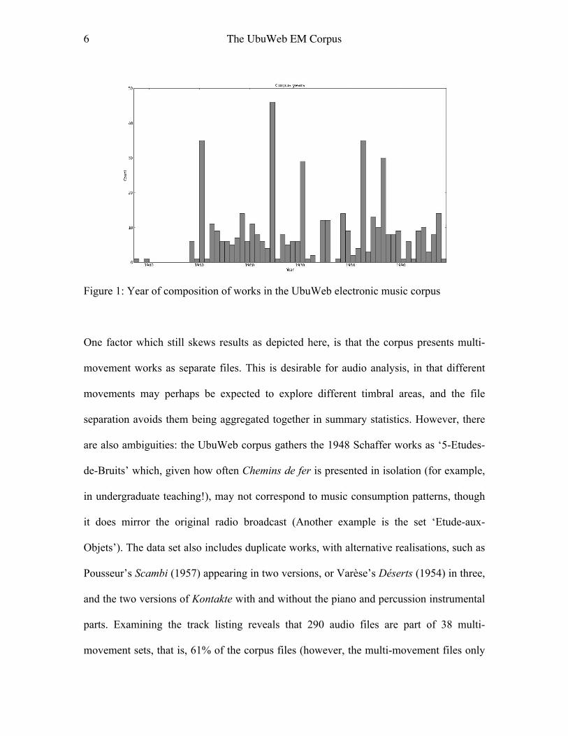
The year of composition of works extends from 1937 to 2000, with a large gap from 1940
to 1947, and no representatives for 1938, 1973 or 1976! Figure 1 provides a histogram by
year of coverage, where the year data from the filenames has been cleaned up. For
example, many works in the UbuWeb corpus have a date presented as a range; in some
cases this is the year of composition and the year of first performance, in others such as
Kontakte it corresponds to a period when the composer was working on a piece; the
correction is to the year of completed composition, so 1960 for Kontakte. Note however
that the years of composition of works in this corpus is by no means as skewed as the
popular music corpus in the Million Song Dataset (Bertin-Mahieux 2011), which is
highly biased to the last decade of coverage (see Figure 3 in ibid.; of songs from 1922 to
2011, the clear peak is around 2006).
6 The UbuWeb EM Corpus
Figure 1: Year of composition of works in the UbuWeb electronic music corpus
One factor which still skews results as depicted here, is that the corpus presents multi-
movement works as separate files. This is desirable for audio analysis, in that different
movements may perhaps be expected to explore different timbral areas, and the file
separation avoids them being aggregated together in summary statistics. However, there
are also ambiguities: the UbuWeb corpus gathers the 1948 Schaffer works as ‘5-Etudes-
de-Bruits’ which, given how often Chemins de fer is presented in isolation (for example,
in undergraduate teaching!), may not correspond to music consumption patterns, though
it does mirror the original radio broadcast (Another example is the set ‘Etude-aux-
Objets’). The data set also includes duplicate works, with alternative realisations, such as
Pousseur’s Scambi (1957) appearing in two versions, or Varèse’s Déserts (1954) in three,
and the two versions of Kontakte with and without the piano and percussion instrumental
parts. Examining the track listing reveals that 290 audio files are part of 38 multi-
movement sets, that is, 61% of the corpus files (however, the multi-movement files only
7 The UbuWeb EM Corpus
account for 33% of the total time duration of the audio). Figure 2 presents years of
compositions where multi-movement and duplicate works are aggregated into single
years. Figure 2 presents a slightly flatter visualisation of the coverage in the corpus,
though the uneven representation of years is still evident, including gaps in the 1970s that
cannot be made up just by aggregating movements of multi-movement works.
Figure 2: Year of composition of works in the UbuWeb electronic music corpus, taking
multi-movement and multi-realisation files into account
One further apparent disadvantage of this corpus is the fact that the audio is provided as
stereo MP3s, with around half at 256 kilobits per second and half at 320 kilobits per
second rate. Use of MP3 format is pragmatic for the distribution of the music from the
server, but raises heckles for audio purists. Double blind experiments have shown the
inability of subjects to discriminate MP3s and uncompressed CD quality audio files
8 The UbuWeb EM Corpus
across multiple music genres at rates of 256 or 320 kbps (and also to not distinguish these
two rates), though lower rates of 192kbps and below are problematic (Pras et al. 2009).
Listening through the corpus reveals that the essential character of the electronic music
works are preserved; since we would expect human analysts to be able to discriminate
and productively examine the works on the basis of the MP3s, so a computer must
ultimately be able to deal with these listening conditions (even if the MP3 are deemed
less than ideal).
Although stereo reduction is imposed in some cases, this is common practice in much
examination of electronic music anyway, given the difficulty of obtaining multitrack
parts for most classic historic works. For analysis, the spatial component is discarded, and
the left and right channels combined as a single mono source (the summation here
assumes there are no major phase cancellation issues in such a procedure). Although
space is an important component of electronic art music (Manning 2013, Harrison and
Wilson 2010), timbre is another such device, and the tools of MIR are well equipped to
tackle timbral information in this corpus; spatial information is omitted from this current
study.
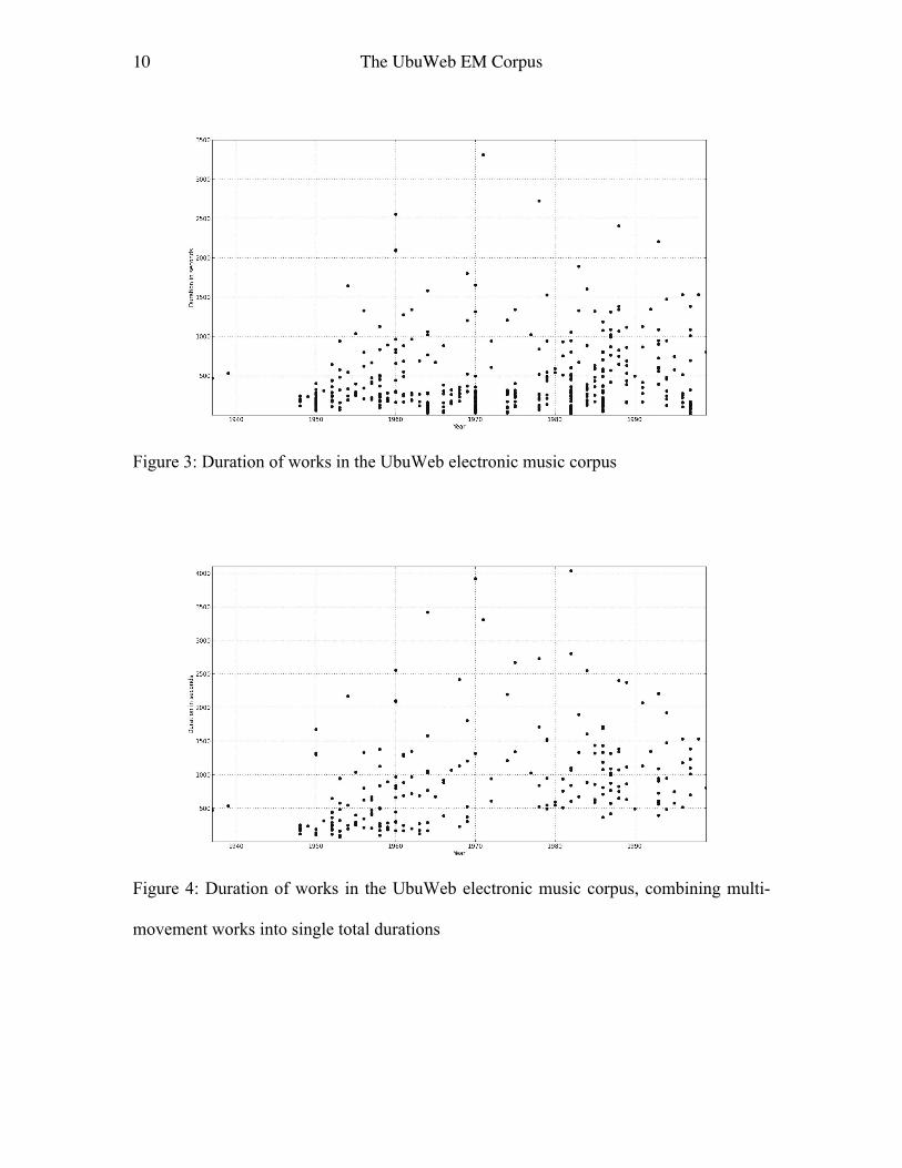
Examining durations of works, Figure 3 presents findings over the corpus across all
individual files, with data points plotted for year of a piece on the x axis and its duration
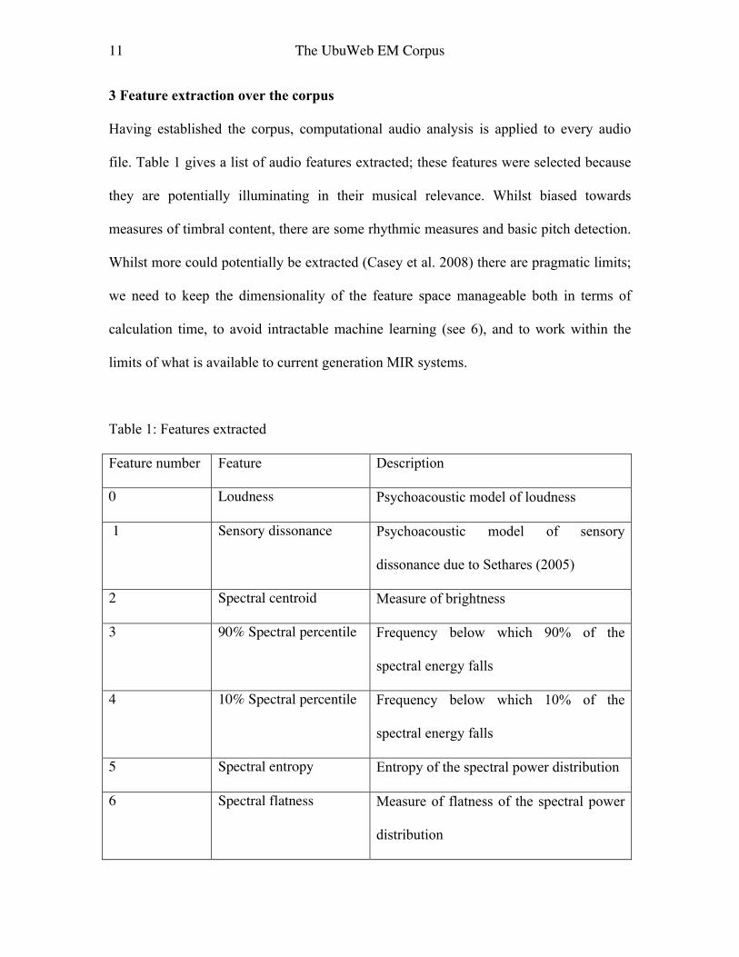
on the y. Figure 4 provides a single total duration for multi-movement works. The longest
single file work is Xenakis’ Persepolis (1971, 55 minutes) but the combined work with
the largest total duration is Philippe Manoury’s Zeitlauf for choir, instrumental ensemble
9 The UbuWeb EM Corpus
and electronics (1982, 67 minutes). Counting multi-movement works by their total
duration, the average duration of works is 14.8 minutes, with a standard deviation of
11.8; using separate movements as separate durations, the average is 7 minutes with a
standard deviation of 7.4 (the duration distribution is of course positive/right skewed
away from zero, so the calculations here reflect the existence of much longer durations
than the mean). Since the repertoire is exclusively art music rather than popular music,
the three minute radio friendly pop single is not represented, and longer works are
unsurprising. There is an arch shape over the whole duration distribution, which points to
smaller studies in earlier years (with some longer multi-movement works composed of
short individual movements) and a reduction in the scale of works in more recent
decades. The former is attributable to the technological challenge of producing early
electronic music, taking many person-hours per minute of audio, with more limited
compositional resources available. Speculating, the latter may be the victim of the
increased number of active composers and the reduced time-per-composer available in
festivals and recordings, though it may also be a quirk of selection bias in the original
formation of the UbuWeb collection. The total corpus duration is 2.3 days of audio.
10 The UbuWeb EM Corpus
Figure 3: Duration of works in the UbuWeb electronic music corpus
Figure 4: Duration of works in the UbuWeb electronic music corpus, combining multi-
movement works into single total durations
11 The UbuWeb EM Corpus
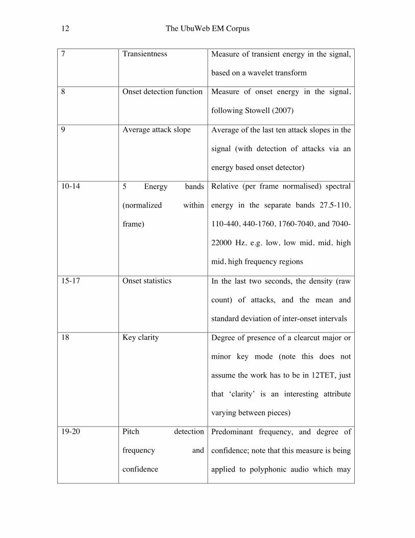
3 Feature extraction over the corpus
Having established the corpus, computational audio analysis is applied to every audio
file. Table 1 gives a list of audio features extracted; these features were selected because
they are potentially illuminating in their musical relevance. Whilst biased towards
measures of timbral content, there are some rhythmic measures and basic pitch detection.
Whilst more could potentially be extracted (Casey et al. 2008) there are pragmatic limits;
we need to keep the dimensionality of the feature space manageable both in terms of
calculation time, to avoid intractable machine learning (see 6), and to work within the
limits of what is available to current generation MIR systems.
Table 1: Features extracted
Feature number Feature Description
0 Loudness Psychoacoustic model of loudness
1 Sensory dissonance Psychoacoustic model of sensory
dissonance due to Sethares (2005)
2 Spectral centroid Measure of brightness
3 90% Spectral percentile Frequency below which 90% of the
spectral energy falls
4 10% Spectral percentile Frequency below which 10% of the
spectral energy falls
5 Spectral entropy Entropy of the spectral power distribution
6 Spectral flatness Measure of flatness of the spectral power
distribution
12 The UbuWeb EM Corpus
7 Transientness Measure of transient energy in the signal,
based on a wavelet transform
8 Onset detection function Measure of onset energy in the signal,
following Stowell (2007)
9 Average attack slope Average of the last ten attack slopes in the
signal (with detection of attacks via an
energy based onset detector)
10-14 5 Energy bands
(normalized within
frame)
Relative (per frame normalised) spectral
energy in the separate bands 27.5-110,
110-440, 440-1760, 1760-7040, and 7040-
22000 Hz, e.g. low, low mid, mid, high
mid, high frequency regions
15-17 Onset statistics In the last two seconds, the density (raw
count) of attacks, and the mean and
standard deviation of inter-onset intervals
18 Key clarity Degree of presence of a clearcut major or
minor key mode (note this does not
assume the work has to be in 12TET, just
that ‘clarity’ is an interesting attribute
varying between pieces)
19-20 Pitch detection
frequency and
confidence
Predominant frequency, and degree of
confidence; note that this measure is being
applied to polyphonic audio which may
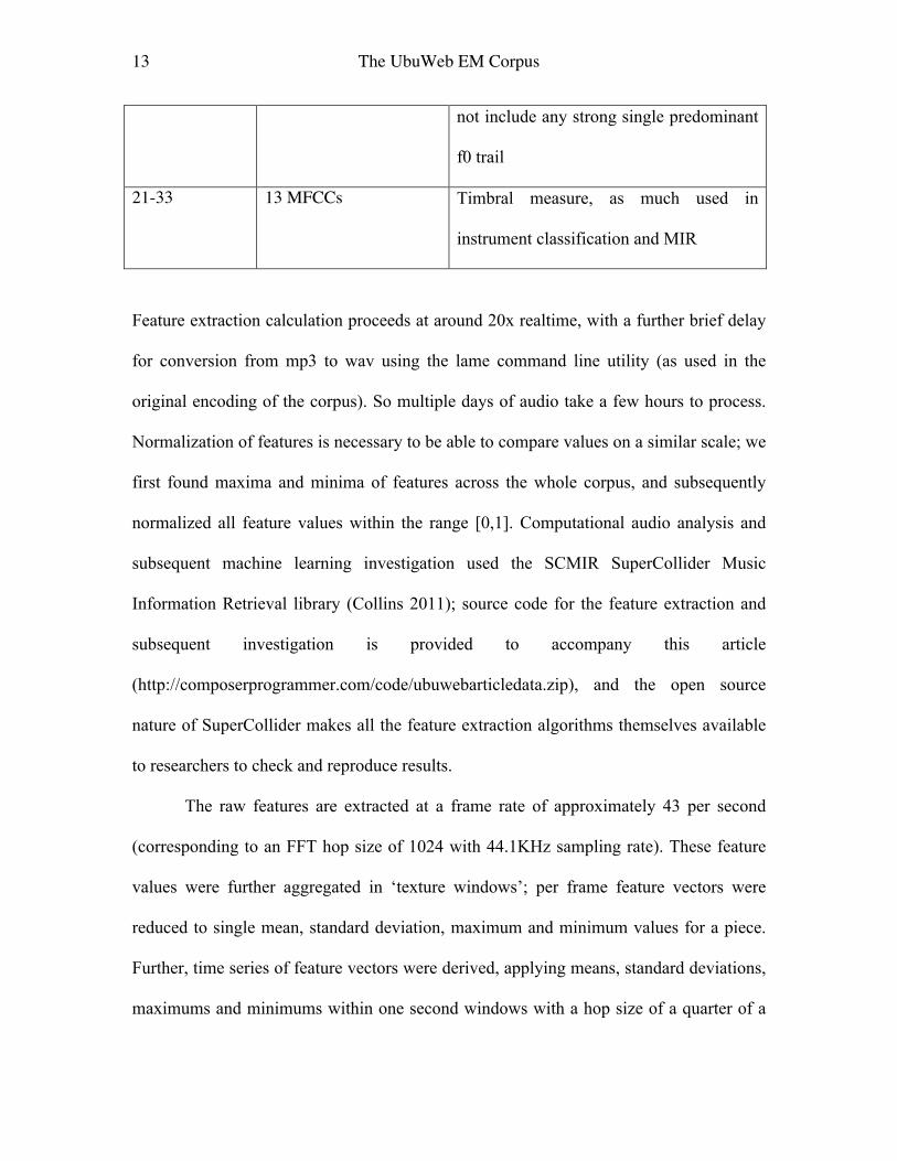
13 The UbuWeb EM Corpus
not include any strong single predominant
f0 trail
21-33 13 MFCCs Timbral measure, as much used in
instrument classification and MIR
Feature extraction calculation proceeds at around 20x realtime, with a further brief delay
for conversion from mp3 to wav using the lame command line utility (as used in the
original encoding of the corpus). So multiple days of audio take a few hours to process.
Normalization of features is necessary to be able to compare values on a similar scale; we
first found maxima and minima of features across the whole corpus, and subsequently
normalized all feature values within the range [0,1]. Computational audio analysis and
subsequent machine learning investigation used the SCMIR SuperCollider Music
Information Retrieval library (Collins 2011); source code for the feature extraction and
subsequent investigation is provided to accompany this article
(http://composerprogrammer.com/code/ubuwebarticledata.zip), and the open source
nature of SuperCollider makes all the feature extraction algorithms themselves available
to researchers to check and reproduce results.
The raw features are extracted at a frame rate of approximately 43 per second
(corresponding to an FFT hop size of 1024 with 44.1KHz sampling rate). These feature
values were further aggregated in ‘texture windows’; per frame feature vectors were
reduced to single mean, standard deviation, maximum and minimum values for a piece.
Further, time series of feature vectors were derived, applying means, standard deviations,
maximums and minimums within one second windows with a hop size of a quarter of a
14 The UbuWeb EM Corpus
second. This kind of reduction is necessary to keep comparisons between pieces tractable,
though there is always the danger that taking statistical descriptors like means or maxima
loses individual information on the distribution and progression of feature values in a
work. That both single summary vectors and time series of texture windows were kept
allays this concern somewhat, and allows comparison of single statistical summary values
versus time series.
Having obtained these derived features, further investigation can look at the
changing values of individual or combined features within and between pieces over
history.
4 Year by year trends
The summary mean, standard deviation and range (maximum-minimum) of feature
values for each piece were plotted against year. A line was fitted to each curve, that is, for
each of the 34 features for each of mean, standard deviation and range. On initial
examination, it appeared that there were no obvious trends in the data; for instance,
loudness values did not indicate an influence in the 1990s for these art music pieces of a
corresponding loudness war in popular music recording (Katz 2007)! On closer
examination of the curves fitted, larger positive or negative gradients were found as in
Table 2.
Table 2: Trends in feature values over years, by largest and smallest gradients of fitted
lines
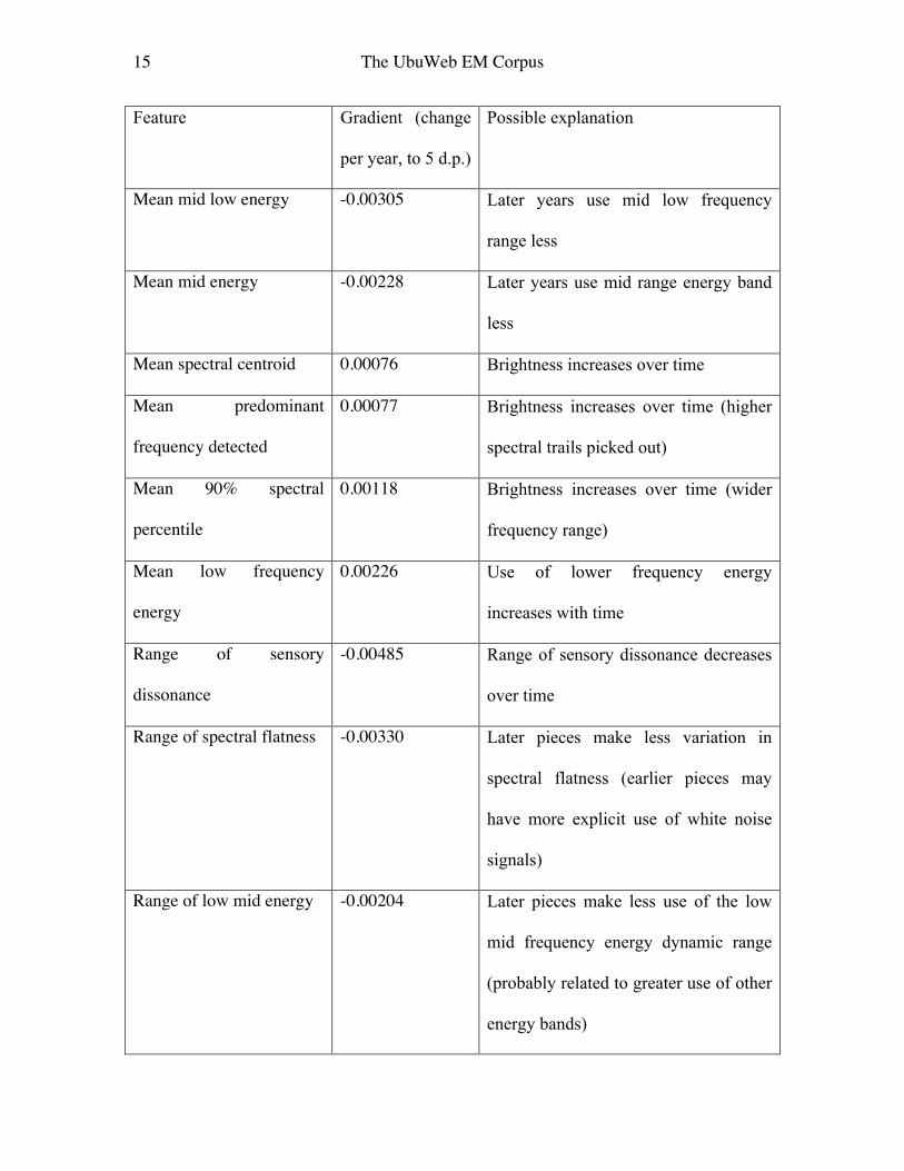
15 The UbuWeb EM Corpus
Feature Gradient (change
per year, to 5 d.p.)
Possible explanation
Mean mid low energy -0.00305 Later years use mid low frequency
range less
Mean mid energy -0.00228 Later years use mid range energy band
less
Mean spectral centroid 0.00076 Brightness increases over time
Mean predominant
frequency detected
0.00077 Brightness increases over time (higher
spectral trails picked out)
Mean 90% spectral
percentile
0.00118 Brightness increases over time (wider
frequency range)
Mean low frequency
energy
0.00226 Use of lower frequency energy
increases with time
Range of sensory
dissonance
-0.00485 Range of sensory dissonance decreases
over time
Range of spectral flatness -0.00330 Later pieces make less variation in
spectral flatness (earlier pieces may
have more explicit use of white noise
signals)
Range of low mid energy -0.00204 Later pieces make less use of the low
mid frequency energy dynamic range
(probably related to greater use of other
energy bands)
16 The UbuWeb EM Corpus
Range of onset detection
energy
0.00314 Later pieces use a greater range of
onset densities
Range of high frequency
energy
0.00957 Later pieces make greater use of high
frequency energy dynamic range
Standard deviation of
spectral entropy
-0.00163 Earlier works historically have a greater
variation in spectral entropy values
Standard deviation of low
mid energy
-0.00154 Earlier works historically have a greater
variation in use of the low mid energy
band
Standard deviation of
sensory dissonance
-0.00099 Earlier works historically have a greater
variation in sensory dissonance (later
works are ‘smoother’ and less ‘rough’
or ‘hard-edged’)
Standard deviation of high
mid frequencies
0.00061 Later works historically have a greater
variation in use of the high mid energy
band
Standard deviation of high
frequencies
0.00068 Later works historically have a greater
variation in use of the high energy band
Standard deviation of low
frequencies
0.00135 Later works historically have a greater
variation in use of the low energy band
The primary trend here is the more restricted use of the whole spectral range in earlier
works; it is clear that earlier recordings have a more restricted spectral compass,
17 The UbuWeb EM Corpus
especially using more of the lower mid band. The reduced frequency range is clear from
listening and checking spectrograms of 1950s tape works (or especially early musique
concrète pre-1951 created using records), though studio recording quality quickly
improved after the first wave of work. Reduced high frequency content and low
frequencies necessarily implies more energy in the middle. However, there were no
corresponding clear trends evident for dynamic range as such; later works are brighter
and have more sub-bass, making more use of low and high frequency bands, but variation
in spectral entropy even reduces over historical time (this may be linked again to usage of
sudden wide-band noise gestures in earlier works, when the technology to produce such
gestures was new, was amongst a more limited set of compositional options, and before
such gestures became too clichéd). Aligned with the reduction in the range of spectral
flatness, this may indicate more explicit use of wide band noise blasts in earlier works, as
exhibited in a work like Pousseur’s Scambi (1957). The table has a few more teasing
indications, such as the greater contrast in onset density within later pieces. Figure 5 plots
mean spectral centroid and 90% spectral percentile energy for all pieces, with the two
fitted line segments superimposed.
18 The UbuWeb EM Corpus
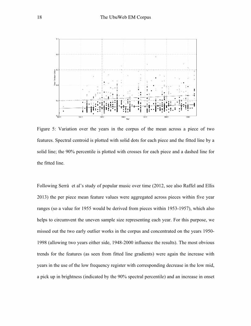
Figure 5: Variation over the years in the corpus of the mean across a piece of two
features. Spectral centroid is plotted with solid dots for each piece and the fitted line by a
solid line; the 90% percentile is plotted with crosses for each piece and a dashed line for
the fitted line.
Following Serrà et al’s study of popular music over time (2012, see also Raffel and Ellis
2013) the per piece mean feature values were aggregated across pieces within five year
ranges (so a value for 1955 would be derived from pieces within 1953-1957), which also
helps to circumvent the uneven sample size representing each year. For this purpose, we
missed out the two early outlier works in the corpus and concentrated on the years 1950-
1998 (allowing two years either side, 1948-2000 influence the results). The most obvious
trends for the features (as seen from fitted line gradients) were again the increase with
years in the use of the low frequency register with corresponding decrease in the low mid,
a pick up in brightness (indicated by the 90% spectral percentile) and an increase in onset
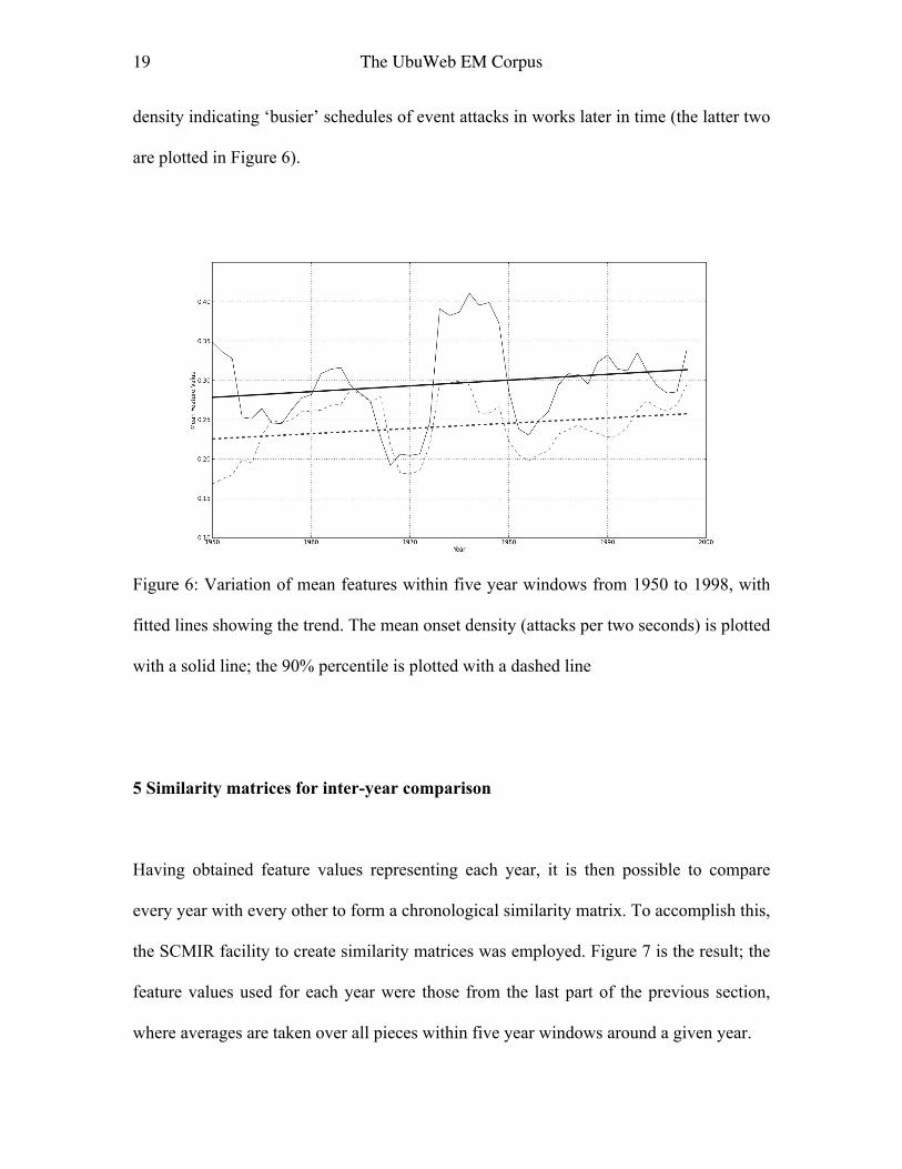
19 The UbuWeb EM Corpus
density indicating ‘busier’ schedules of event attacks in works later in time (the latter two
are plotted in Figure 6).
Figure 6: Variation of mean features within five year windows from 1950 to 1998, with
fitted lines showing the trend. The mean onset density (attacks per two seconds) is plotted
with a solid line; the 90% percentile is plotted with a dashed line
5 Similarity matrices for inter-year comparison
Having obtained feature values representing each year, it is then possible to compare
every year with every other to form a chronological similarity matrix. To accomplish this,
the SCMIR facility to create similarity matrices was employed. Figure 7 is the result; the
feature values used for each year were those from the last part of the previous section,
where averages are taken over all pieces within five year windows around a given year.
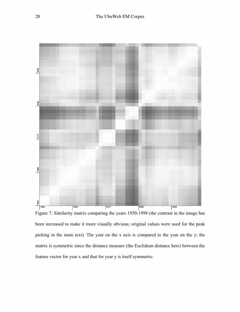
20 The UbuWeb EM Corpus
Figure 7: Similarity matrix comparing the years 1950-1998 (the contrast in the image has
been increased to make it more visually obvious; original values were used for the peak
picking in the main text). The year on the x axis is compared to the year on the y; the
matrix is symmetric since the distance measure (the Euclidean distance here) between the
feature vector for year x and that for year y is itself symmetric.
21 The UbuWeb EM Corpus
One clear aspect of this matrix is the band showing how the period 1976-1979 is
generally different to other years in the corpus (the black band leading out horizontally
and vertically showing the relation of these years to all others). This may appear to be an
artefact of the lack of representatives for 1976; though the five year window also
dampens out that effect, the 1970s have a reduced number of works overall (see Figure
1). In searching for actual works that may stand out here, Xenakis’ La Légende D’Eer
(1978) and Chowning’s Stria (1977) might be proposed as sufficiently different to
everything else in the corpus to account for this effect, though Xenakis’ Gendy3 and
other Chowning works are also present in other years.
Given a similarity matrix, it is possible to look for larger than normal transitions from one
year to the next. The standard MIR method uses convolution with a checkerboard kernel
along the matrix diagonal (Casey et al. 2008) to look for larger changes from one self-
similar area to a new and different self-similar area (you can see this in Figure 7 as the
checkerboard like patterns along the maximally self-similar bottom left to top right
diagonal). A novelty curve can be created showing the changes over time from year to
year, and then peak picked for particularly prominent years of change. Running this, the
years of greatest change were 1952, 1972, 1973, 1979, 1980 and 1981; on examination of
the matrix in Figure 7 and the novelty curve, these reduce to 1952, 1972 and 1980.
Whereas there is a strong historical reason to explain 1952 as an interesting transition
point given the establishing of elektronisches Musik after previous experiments in
musique concrète, 1972 and 1980 appear more mysterious. 1972 is only represented by
two works in the corpus, one of which is Chowning’s Turenas, which might be said to
22 The UbuWeb EM Corpus
form a major innovation (not withstanding Risset’s 1969 Mutations which more modestly
employed the FM algorithm, and is in the UbuWeb corpus).
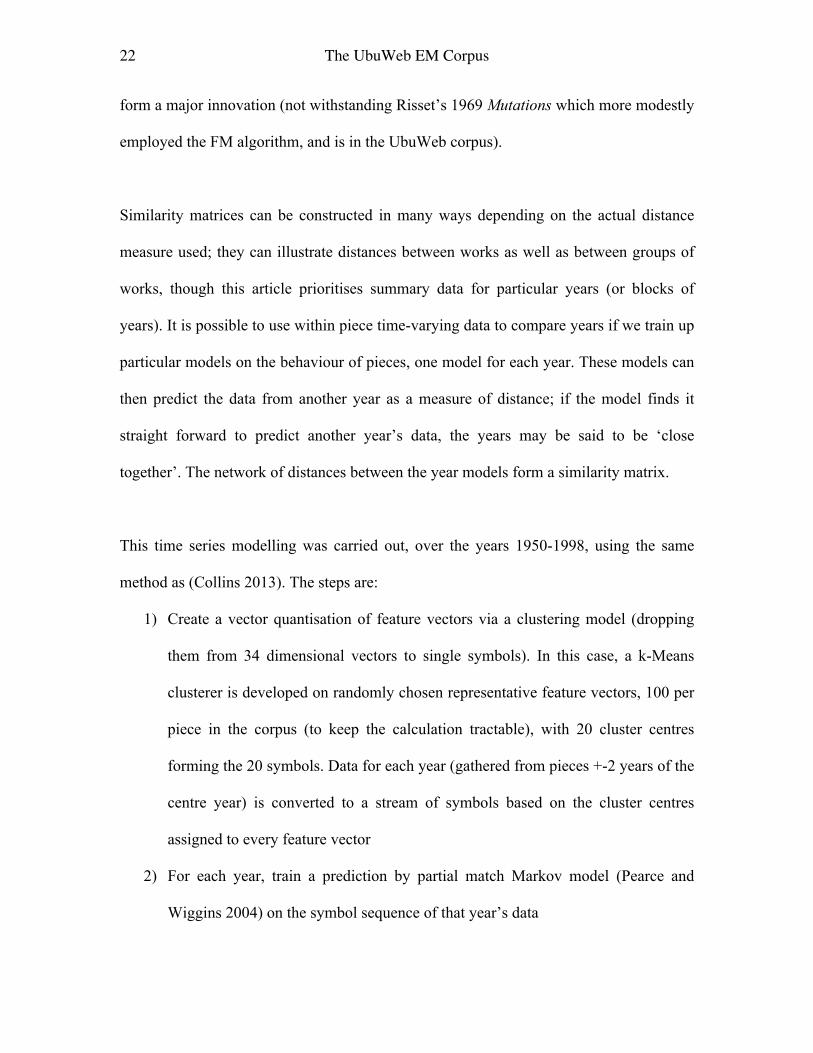
Similarity matrices can be constructed in many ways depending on the actual distance
measure used; they can illustrate distances between works as well as between groups of
works, though this article prioritises summary data for particular years (or blocks of
years). It is possible to use within piece time-varying data to compare years if we train up
particular models on the behaviour of pieces, one model for each year. These models can
then predict the data from another year as a measure of distance; if the model finds it
straight forward to predict another year’s data, the years may be said to be ‘close
together’. The network of distances between the year models form a similarity matrix.
This time series modelling was carried out, over the years 1950-1998, using the same
method as (Collins 2013). The steps are:
1) Create a vector quantisation of feature vectors via a clustering model (dropping
them from 34 dimensional vectors to single symbols). In this case, a k-Means
clusterer is developed on randomly chosen representative feature vectors, 100 per
piece in the corpus (to keep the calculation tractable), with 20 cluster centres
forming the 20 symbols. Data for each year (gathered from pieces +-2 years of the
centre year) is converted to a stream of symbols based on the cluster centres
assigned to every feature vector
2) For each year, train a prediction by partial match Markov model (Pearce and
Wiggins 2004) on the symbol sequence of that year’s data
23 The UbuWeb EM Corpus
3) Form a similarity matrix where the distance(A,B) is the symmetric cross
likelihood: the score for the model for year A’s prediction of the data for year B is
combined with the model for year B’s prediction of the data for year A and the
models’ self scores (A predict’s A’s training data, model B predicts data B)
(Virtanen and Helén 2007)
Figure 8 plots results, which again show a banding around the years 1973-1980 placing
them in contrast to other years in the corpus. The amount of (post k-Means symbolic)
data representing each decade is not massively different, though it is least for the 1970s
and expanded for the 1980s (1950s: 674764 symbols, 1960s: 727708, 1970s: 556061,
1980s:1203307, 1990s: 641821). Novelty curve analysis pointed to the years 1955, 1968,
1972 and 1993 as possible transition points; no further speculation is undertaken at this
point except to corroborate the appearance of 1972, though the reader can observe that
different numerical methods may lead to different years being highlighted (parameters of
the peak picking and the window for the novelty curve generation also play a part).
24 The UbuWeb EM Corpus
Figure 8: Similarity matrix from symbolic model predictions comparing the years 1950-
1998
6 Machine learning
It can be further illuminating to apply machine learning algorithms to the corpus data.
Given annotated years, or some other derived label such as the decade of composition, a
25 The UbuWeb EM Corpus
supervised machine learning task would be to train a predictor which can predict the year
of composition. Where this proves to be a difficult task, it may provide evidence that the
feature extraction is not sufficiently discriminatory, or if we are willing to trust that the
feature extraction is basically effective, that the task is inherently difficult (and that there
is a strong musical overlap across years).
Unsupervised algorithms can assist in seeing how the data falls ‘naturally’, at
least according to the algorithm, without prior knowledge of date labels. One problem is
that the feature extraction presented here places works within a 34-dimensional space; in
order to visualise and interpret results, some kind of dimension reduction (herein to two
dimensions) must be applied to facilitate plotting.
We now explore the former supervised task by training classifiers and the latter
by Multi-Dimensional Scaling (MDS). Calculation used a combination of SuperCollider
implementations for the former, and python (from the sklearn package) for the latter; all
source code, including for plotting, accompanies this article. There are many more
algorithms that could have been deployed (for instance the unsupervised task could be
approached with a self organising map, the supervised with a support vector machine or
many other well known algorithms), so this section is merely a taster of possibilities.
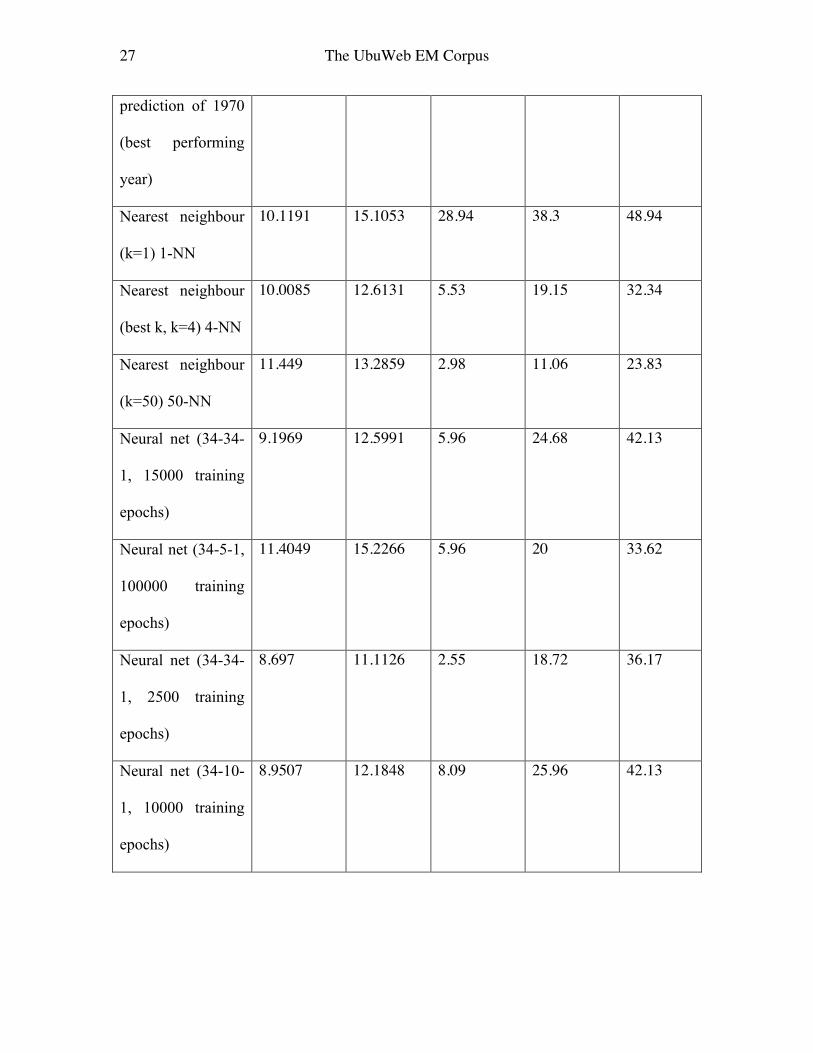
6.1 Year prediction
We can attempt to predict the year of the works in the corpus using supervised machine
learning. Half the corpus (randomly selected) was used as a training set, and assessment
of the quality of prediction was carried out on a test set of the remaining half. In the paper
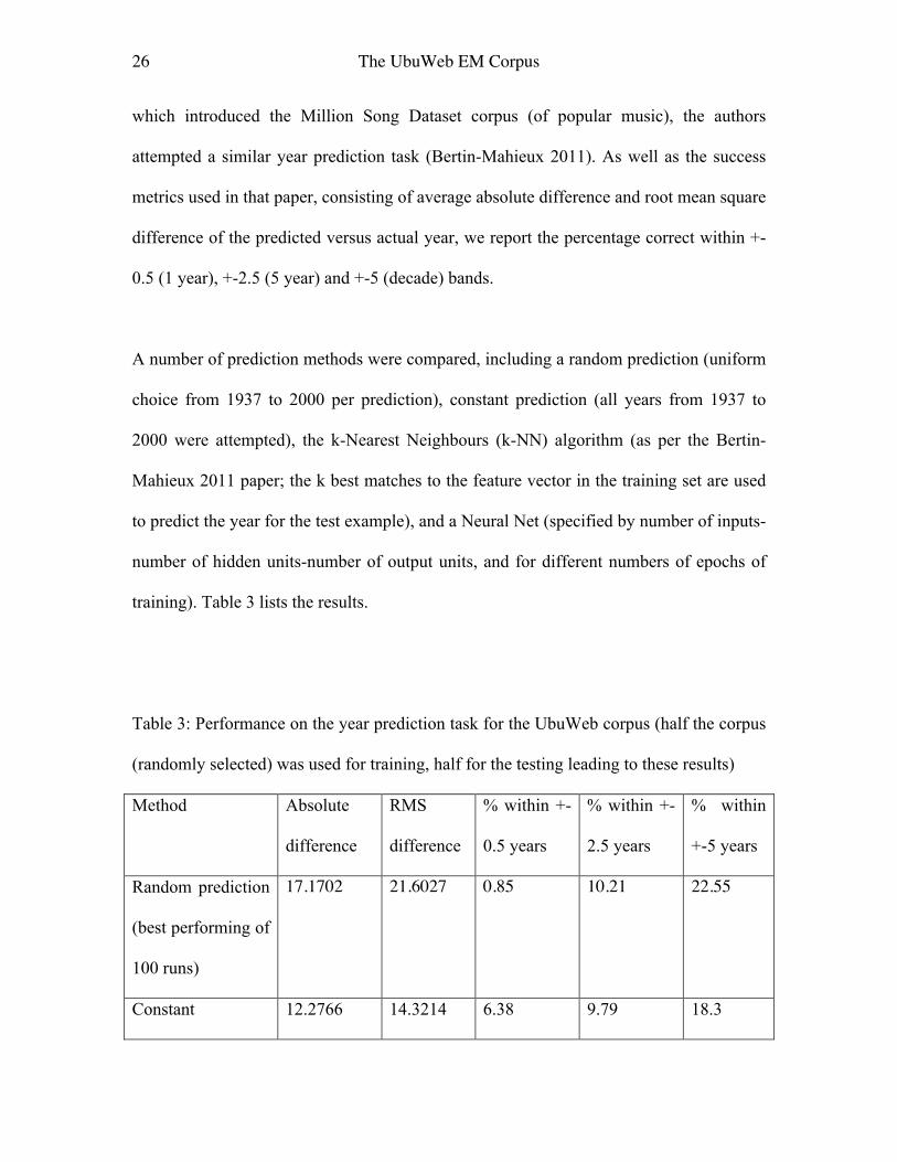
26 The UbuWeb EM Corpus
which introduced the Million Song Dataset corpus (of popular music), the authors
attempted a similar year prediction task (Bertin-Mahieux 2011). As well as the success
metrics used in that paper, consisting of average absolute difference and root mean square
difference of the predicted versus actual year, we report the percentage correct within +-
0.5 (1 year), +-2.5 (5 year) and +-5 (decade) bands.
A number of prediction methods were compared, including a random prediction (uniform
choice from 1937 to 2000 per prediction), constant prediction (all years from 1937 to
2000 were attempted), the k-Nearest Neighbours (k-NN) algorithm (as per the Bertin-
Mahieux 2011 paper; the k best matches to the feature vector in the training set are used
to predict the year for the test example), and a Neural Net (specified by number of inputs-
number of hidden units-number of output units, and for different numbers of epochs of
training). Table 3 lists the results.
Table 3: Performance on the year prediction task for the UbuWeb corpus (half the corpus
(randomly selected) was used for training, half for the testing leading to these results)
Method Absolute
difference
RMS
difference
% within +-
0.5 years
% within +-
2.5 years
% within
+-5 years
Random prediction
(best performing of
100 runs)
17.1702 21.6027 0.85 10.21 22.55
Constant 12.2766 14.3214 6.38 9.79 18.3
27 The UbuWeb EM Corpus
prediction of 1970
(best performing
year)
Nearest neighbour
(k=1) 1-NN
10.1191 15.1053 28.94 38.3 48.94
Nearest neighbour
(best k, k=4) 4-NN
10.0085 12.6131 5.53 19.15 32.34
Nearest neighbour
(k=50) 50-NN
11.449 13.2859 2.98 11.06 23.83
Neural net (34-34-
1, 15000 training
epochs)
9.1969 12.5991 5.96 24.68 42.13
Neural net (34-5-1,
100000 training
epochs)
11.4049 15.2266 5.96 20 33.62
Neural net (34-34-
1, 2500 training
epochs)
8.697 11.1126 2.55 18.72 36.17
Neural net (34-10-
1, 10000 training
epochs)
8.9507 12.1848 8.09 25.96 42.13
28 The UbuWeb EM Corpus
In contrast to Bertin-Mahieux (2011) the 1-NN classifier performed better than the 50-
NN; it is good to see that there is some local regularity of feature vectors allowing the
closest vector to predict the year, pointing to some consistency of sound world from year
to year over composers and studios. Averaging the 50 nearest years however, especially
given the smaller size of the corpus, is ineffective; a search across all k from 1 to 50
found the best performing (at least in terms of the difference scores) for k=4, though the
best percentages were for k=1. Indeed, the 1-NN method out performs in percentages the
best found neural net, though the neural nets had much better difference scores when they
didn’t over-fit the training set. That the classifiers do not perform above 50% accuracy
even as to the decade further indicates the heterogeneity of the corpus. Nonetheless, the
1-NN results, and the performance far above chance in general, point to some relation
between detail captured and summarised with audio features and different years of
composition.
It is also possible to attempt a simpler and easier task, to predict the ‘era’ of a piece. In
this case, we consider two time spans; before 1972, and 1972 and afterwards (motivated
by the appearance of 1972 as a possible important boundary in the corpus from earlier
sections of this article). This two class classification problem can be solved at 50%
accuracy by chance, and a constant guess of always predicting a piece originates before
1972 is 55.32% (since 55.32% of pieces have dates preceding 1972). 1-NN performs at
71.06% (the best k=1 again), and a neural net was quickly trained to operate at 79.15%
effectiveness (34-34-1, 500 epochs training; more epochs tended to inhibit
generalisation). These results are again indicative that there is evolution over time in the
29 The UbuWeb EM Corpus
timbral nature of pieces sufficient to partially discriminate different eras, though the
feature extraction (or the fundamental task itself) remains unable to discriminate the
chronological origin of pieces given two options, at 80% or greater effectiveness.
Though a human study may be interesting on this task, any human expert would be
expected to recognise a priori many works from the corpus, and the machine analysis
here provides a more objective take on the problem, whilst pointing to problems of its
own in the discriminatory power or otherwise of the feature extraction employed.
6.2 Multi dimensional scaling to plot piece and year proximities
Multi-dimensional scaling (MDS) allows a low dimensional plot to be made from a
similarity matrix, that is, from an exhaustive set of distances between objects, as
famously used in perceptual studies in sound timbre (Risset and Wessel 1999). Since
similarity matrices are exactly what were created in section 5, it is straight forward to
explore MDS; the python module sklearn was used to run MDS and matplotlib to plot
figures once SuperCollider had generated the distance matrices and output them as csv
files.
Figure 9 plots by-year data where each year was represented by a mean feature vector
and a dissimilarity distance matrix formed by taking Euclidean distances. Whilst some
years naturally separate, such as the early 1950s, the overall separation is not that clean,
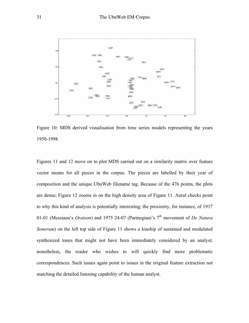
pointing to the problem of representation by a statistical mean alone. Figure 10, however,
uses the similarity matrix formed from the predictive models (as per the time series
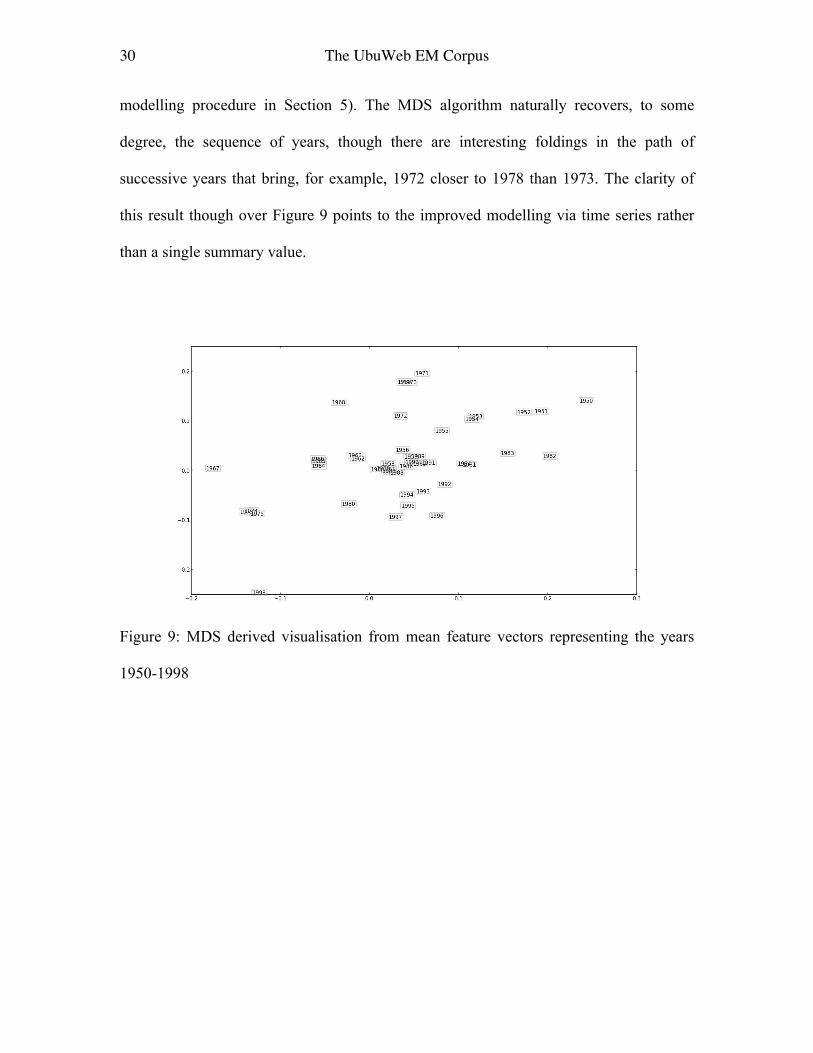
30 The UbuWeb EM Corpus
modelling procedure in Section 5). The MDS algorithm naturally recovers, to some
degree, the sequence of years, though there are interesting foldings in the path of
successive years that bring, for example, 1972 closer to 1978 than 1973. The clarity of
this result though over Figure 9 points to the improved modelling via time series rather
than a single summary value.
Figure 9: MDS derived visualisation from mean feature vectors representing the years
1950-1998
31 The UbuWeb EM Corpus
Figure 10: MDS derived visualisation from time series models representing the years
1950-1998
Figures 11 and 12 move on to plot MDS carried out on a similarity matrix over feature
vector means for all pieces in the corpus. The pieces are labelled by their year of
composition and the unique UbuWeb filename tag. Because of the 476 points, the plots
are dense; Figure 12 zooms in on the high density area of Figure 11. Aural checks point
to why this kind of analysis is potentially interesting; the proximity, for instance, of 1937
01-01 (Messiaen’s Oraison) and 1975 24-07 (Parmegiani’s 7th movement of De Natura
Sonorum) on the left top side of Figure 11 shows a kinship of sustained and modulated
synthesized tones that might not have been immediately considered by an analyst;
nonetheless, the reader who wishes to will quickly find more problematic
correspondences. Such issues again point to issues in the original feature extraction not
matching the detailed listening capability of the human analyst.
32 The UbuWeb EM Corpus
Figure 11: MDS derived visualisation across all 476 pieces in the UbuWeb corpus, via
the similarity matrix over the mean feature vector
Figure 12: MDS derived visualisation across all 476 pieces in the UbuWeb corpus, via
the similarity matrix over the mean feature vector, zoomed in on the high density area
33 The UbuWeb EM Corpus
7 Discussion
Trusting computer-automated audio analysis means accepting that the feature extraction
provides musical description that is psychologically relevant to human listeners, and
indeed, captures a musical analyst’s aural experience. It is a leap to claim understanding
on the part of the computer to any comparable degree to a human listener. Technical
development and psychological validation of machine listening technology is an ongoing
research field, and this article has pointed at a number of places to underlying discontent
with the feature extraction utilised. Though there is gathering interest amongst electronic
music scholars in automated methods for analysis (Klein et al. 2012, Park et al. 2009), the
current study shows the mixed results available with current generation machine
listening, whatever the benefits of objective reproducible research and tireless analysis. A
too preliminary conclusion that, for example, electronic art music history is rather
homogenous, may only point to the lack of discriminatory power of the feature extraction
methodology; fortunately, even current generation tools point to some variation over
time. Though suggestive, trends over time as presented herein are indications for further
study, and not definitive discoveries.
The UbuWeb corpus has issues as a resource that go beyond the methods of analysis,
though at least it is publicly available! It is well known that problems with meta-data are
common in creating larger corpuses. Errors in the formation of a data set have an impact
on MIR studies, as the work of Bob Sturm on the Tzanetakis data set used in genre
recognition evaluation has ably demonstrated (Sturm 2012). With the UbuWeb corpus,
34 The UbuWeb EM Corpus
problems include dates in filenames, the status of multi-movement works, and the
coverage of the original selection. In working with the corpus, further quirks found
include a three minute spoken radio concert introduction (Presentation du Concert de
Bruits), the long round of applause at the close of Cage’s Williams Mix, a 12 second
silent track accompanying Berio’s Chants Parallèles, further silence in an accompanying
track to James Dashow’s Mnemonics for violin and computer and two minutes of the last
movement of Stockhausen’s Mixtur, a different filename labelling on the last 9 tracks of
the corpus (61_01 to 61_09) and Chowning’s Phone appearing twice!
The UbuWeb corpus cannot claim, therefore, to be the most carefully controlled and
representative gathering of electronic music works (the original creation of the collection
did not bear in mind the automatic analysis to it has been subjected here). Despite its
flaws, analysis here has pointed to some interesting facets of the development of
electronic art music, and scholars of electronic music may continue to find much of use in
the corpus, hopefully including through code and results gained in the present study.
Future work will, however, also seek to build a more carefully representative corpus or
corpora, better controlled for such factors as gender balance, year of composition,
coverage of electronic music styles (especially beyond pure art music), and limiting the
influence of acoustic instrument works with only a small electronic component. The
treatment of multi-movement works will remain a concern in any new corpus study, since
it would deny an extensive critical literature to bar a longer work such as Kontakte. If
research questions concern differences between works as a whole, or between composers,
35 The UbuWeb EM Corpus
or between years, particular aggregation of movements and pieces can be conducted at
the analysis software stage as long as the database itself is appropriately marked up (the
meta-data accompanying audio must indicate the nature of groupings of individual audio
files within a multi-movement form). In certain cases, an extract, a few movements or a
single movement might be claimed representative of a longer multi-section work, though
any unity of conception of long and multi-movement works would stand in danger of
being lost. Further, the current study has sidestepped the extensive issues of spatial
sound, by treating timbre as primary and all sources as mono (through channel summed
stereo). Addressing spatial movement will require new analysis machinery, at the very
least, extraction of per channel features, and then the means to track perceptually relevant
movement within the spatial field taking multiple and all channels into account. That
different spatialization set-ups are assumed by different works is a major challenge for
future research.
All of this points to how much there remains to do in working with larger data sets of
electronic music. Ultimately, we might hope to create tools which can in some sense
‘save the human analyst’ from listening through massive collections of audio, addressing
specific musicological research questions, and which we can trust as our proxies.
Machine-led audio analysis has the potential to exceed, at least in objectivity and
continuous vigour, the human analyst. Yet the human analyst will only trust those
processes that have been thoroughly vetted and validated; the present study is but a
starting point in the kind of critically aware work with computational tools that must be
undertaken to approach this. There may or may not be a fully trustworthy replacement,
36 The UbuWeb EM Corpus
but seeking the computerised musicologist is an undertaking that teaches us a huge
amount about the processes and limits of analysis itself and the biases of the human
scholar, provides an immensely productive research challenge in machine listening and
computer music, and gives a unique handle on large corpora including historical
development in electronic music that would not be possible by other means.
References
Bertin-Mahieux, T., Ellis, D. P.W., Whitman, B. and Lamere, P. (2011)
The Million Song Dataset. Proceedings of the 12th International Society
for Music Information Retrieval Conference.
Casey, M. A., Veltkamp, R., Goto, M., Leman, M., Rhodes, C. and Slaney, M. (2008)
Content-based music information retrieval: Current directions and future challenges.
Proceedings of the IEEE 96(4): 668–96.
Clarke, E. and Cook, N. (eds) (2004). Empirical Musicology: Aims, Methods, Prospects.
Oxford: Oxford University Press.
Collins, N. (2011) SCMIR: A SuperCollider Music Information Retrieval Library.
Proceedings of the International Computer Music Conference: 499–502.
37 The UbuWeb EM Corpus
Collins, N. (2013) Noise Music Information Retrieval. pp. 79-98 in Cassidy, A. and
Einbond, A. (eds.) Noise in and as music. University of Huddersfield, Huddersfield.
ISBN 978-1-86218-118-2
Griffiths, P. (1979) A Guide to Electronic Music. London: Thames and Hudson.
Harrison, J. and Wilson, S. (eds.) (2010) Sound <–> Space: New approaches to
multichannel music and audio. Organised Sound 15(3)
Katz, B. (2007). Mastering Audio: The Art and the Science (2nd Ed.). Oxford: Focal
Press
Klien, V., Grill, T., and Flexer, A. (2012) On Automated Annotation of Acousmatic
Music. Journal of New Music Research 41(2): 153–73.
Landy, L. (2007). Understanding the Art of Sound Organisation. Cambridge, MA: MIT
Press
Manning, P. (2013) Electronic and Computer Music (4th Ed.). New York: Oxford
University Press
Marsden, A. and Pople, A. (eds.) (1992). Computer Representations and Models in
Music. London: Academic Press.
38 The UbuWeb EM Corpus
Park, T. H., Li, Z. and Wu, W. (2009) EASY does it: The Electro-Acoustic music
analYsis toolbox. Proceedings of the International Symposium on Music Information
Retrieval, Kobe, Japan
Pearce, M. and Wiggins, G. (2004) Improved methods for statistical modelling of
monophonic music. Journal of New Music Research 33(4): 367–85.
Pras, A., Zimmerman, R., Levitin, D., and Guastavino, C. (2009) Subjective evaluation of
MP3 compression for different musical genres. In Audio Engineering Society Convention
127, Audio Engineering Society.
Raffel, C. and Ellis, D. (2013) Reproducing Pitch Experiments in “Measuring the
Evolution of Contemporary Western Popular Music”. Research report. Available from
http://rrr.soundsoftware.ac.uk/reproducing-pitch-experiments-measuring-evolution-
contemporary-western-popular-music
Risset, J.-C. and Wessel, D. L. (1999). Exploration of timbre by analysis and synthesis.
pp. 113–69 in Deutsch, D. (ed.) (1999). The Psychology of Music (2nd Edition). San
Diego, CA: Academic Press
Selfridge-Field, E. (1993). Music analysis by computer. pp. 3–24 in Haus, G. (ed.)
(1993). Music Processing. Oxford: Oxford University Press.
39 The UbuWeb EM Corpus
Serrà, J., Corral, Á., Boguñá, M., Haro, M. and Arcos, J. L. (2012) Measuring the
evolution of contemporary western popular music. Scientific reports 2
Sethares, W. A. (2005) Tuning Timbre Spectrum Scale (2nd Ed.) Berlin: Springer Verlag
Stowell, D., and Plumbley, M. D. (2007) Adaptive whitening for improved real-time
audio onset detection. In Proceedings of the International Computer Music Conference,
Copenhagen, Denmark: 312-319.
Sturm, B. (2012) An Analysis of the GTZAN Music Genre Dataset. Proceedings of the
second international ACM workshop on Music information retrieval with user-centered
and multimodal strategies, pp. 7-12
Virtanen, T. and Helén, M. (2007) Probabilistic model based similarity measures for
audio query-by-example. Proceedings of the IEEE Workshop on Applications of Signal
Processing to Audio and Acoustics, New York: 82–85.
Wiggins, G., Miranda, E., Smaill, A. and Harris, M. (1993). A framework for the
evaluation of music representation systems. Computer Music Journal 17(3):31–42.