Multiresolution network models

Bailey K. Fosdick∗

Colorado State University

Tyler H. McCormickUniversity of Washington

Thomas Brendan MurphyUniversity College Dublin

Tin Lok James NgUniversity College Dublin

Ted WestlingUniversity of Washington

Abstract

Many existing statistical and machine learning tools for social network analysis fo-cus on a single level of analysis. Methods designed for clustering optimize a globalpartition of the graph, whereas projection based approaches (e.g. the latent spacemodel in the statistics literature) represent in rich detail the roles of individuals. Manypertinent questions in sociology and economics, however, span multiple scales of analy-sis. Further, many questions involve comparisons across disconnected graphs that will,inevitably be of different sizes, either due to missing data or the inherent heterogeneityin real-world networks. We propose a class of network models that represent networkstructure on multiple scales and facilitate comparison across graphs with different num-bers of individuals. These models differentially invest modeling effort within subgraphsof high density, often termed communities, while maintaining a parsimonious structurebetween said subgraphs. We show that our model class is projective, highlighting anongoing discussion in the social network modeling literature on the dependence of in-ference paradigms on the size of the observed graph. We illustrate the utility of ourmethod using data on household relations from Karnataka, India.

Keywords: latent space, multiscale, projectivity, social network, stochastic blockmodel

1 Introduction

Social network data consist of a sample of actors and information on the presence/absence of

pairwise relationships among them. These data are often represented as a graph where nodes

∗Authors listed in alphabetical order. Contact emails: bailey.fosdick@colostate.edu and tylermc@uw.edu.

1

arX

iv:1

608.

0761

8v5

[st

at.M

E]

5 J

ul 2

018

correspond to actors and edges (ties) connect nodes with a relationship. A relationship may

represent, for example, friendship between students, co-authorship between academics on a

journal article, or a financial transaction between organizations. Understanding structure in

social networks is essential to appreciating the nuances of human behavior and is an active

area of research in the social sciences (Borgatti et al., 2009). Existing statistical models for

social networks typically focus on either (i) carefully representing structure among actors

that have a relatively high likelihood of interaction, or (ii) clearly differentiating between

groups of actors, i.e. communities, within the graph that have high within-group connectivity

and low between-group connectivity (see e.g. Salter-Townshend et al. (2012) for a review).

Unfortunately, neither of these approaches fully characterize the complexities displayed in

many real-world social networks.

Observed graphs frequently exhibit a mixture structure that manifests through a combi-

nation of global sparsity and local density. Global sparsity implies that the propensity for a

tie between any two randomly selected actors is incredibly small. Yet, massive heterogeneity

in the propensity for actors to connect often creates local graph structure concentrated in

dense subgraphs, frequently termed communities. This structure is typically particularly

pronounced in very large graphs. For example, in the context of online communication

networks, Ugander et al. (2011) describe the Facebook graph as containing pockets of “sur-

prisingly dense” structure, though overall the graph is immensely sparse.

In this paper, we propose a multiresolution model for capturing heterogeneous, complex

structure in social networks that exhibit strong community structure. Our modeling frame-

work decomposes network structure into a component that describes between-community

relations, i.e. relations between actors belonging to different communities, and another com-

ponent describing within-community relations. The proposed framework has two distinct

advantages over existing methods. First, our framework is able to accommodate a wide va-

riety of models for between- and within-community relations. This feature allows the model

to be tailored to reflect different scientific questions that arise when exploring the behavior

2

within and across these communities. The second advantage of our model is that it balances

parsimony with model richness by selectively directing modeling efforts towards representing

interesting, relevant network structure. Typically, this structure is found within actors’ local

communities. In such cases, we can exert the most modeling effort (i.e. model complexity

and computational effort) within dense pockets, where we expect the most complex depen-

dence structure, and use a parsimonious model to capture between community patterns. A

similar approach has been adopted in spatial statistics where locations are partitioned into

disjoint dependence neighborhoods (Page and Quintana, 2016). Compared to popular net-

work models that capture global structure, our approach can provide increased resolution on

intricate structure within communities. Furthermore, our model is able to apportion little

effort to modeling simple structure, resulting in a model that is substantially less complex

than existing models focused on local structure for networks, even with only a few hundred

actors.

After defining our model framework, we discuss its statistical properties. In exploring

these properties, we take a traditional sampling perspective and consider our observed net-

work as that pertaining to a collection of actors sampled from an infinite population of

actors. Our goal is to learn features of the infinite population from the observed graph.

In our model, these features include the distribution of within-community structure across

the network. Communities are defined by their structure and may not have a consistent

size. Therefore, inference about the population-level parameters requires that we be able to

coherently compare and summarize parameters associated with subgraphs of different sizes.

We may also desire to compare network-level parameters to those from another network of

a different size and a different number of communities. In order for these properties to hold

and comparisons to be meaningful, the model class must be a projective family, in the “con-

sistency under sampling” sense of Shalizi and Rinaldo (2013). We introduce this concept

and show the class of multiresolution network models proposed have this property. We also

discuss the important implications of this for population inference.

3

In the remainder of this section, we explore the two existing approaches to multiresolution

modeling of networks, highlighting their strength and weaknesses. In Section 2, we introduce

the general form of our multiresolution modeling framework, and in Section 3 we present one

of many possible model instantiations, called the Latent Space Stochastic Blockmodel (LS-

SBM). Section 4 describes the projectivity properties of this framework and provides context

through comparison with other available methods. Finally, we conclude with a discussion in

Section 5.

1.1 Related models

In this section, we describe two existing models, the Latent Position Cluster Model (Hand-

cock et al., 2007) and the Locally Dependent Exponential Random Graph Model (Schwein-

berger and Handcock, 2014), which capture aspects of our multiresolution approach.

The Latent Position Cluster Model (LPCM) of Handcock et al. (2007) is an extension

of the latent geometry framework introduced in Hoff et al. (2002), where the probability of

network ties is a function of the distance between actor positions in a latent space. The

LPCM performs model-based clustering (Fraley and Raftery, 2002) on the positions in the

unobserved social space. Cluster memberships then capture group structure and within-

group analysis is performed by examining the actor-specific latent positions within each

cluster. The likelihood for the LPCM, like that for the original latent space models, requires

estimating a distance between every two pair of actors in the unobserved social space. In

even moderately large graphs, these distance calculations are computationally expensive and

the propensity for actors in different groups to interact is often very small. In addition, since

both ties and non-ties are weighted equally by the LPCM, the latent position for each node

is heavily influenced by the numerous other nodes with which it has no relation.

An attractive property of the LPCM is that it parsimoniously encodes patterns among

ties in the network using a low-dimensional structure. As a consequence of this, the model

tie probabilities are constrained by the latent geometry. Often these constraints are seen as

4

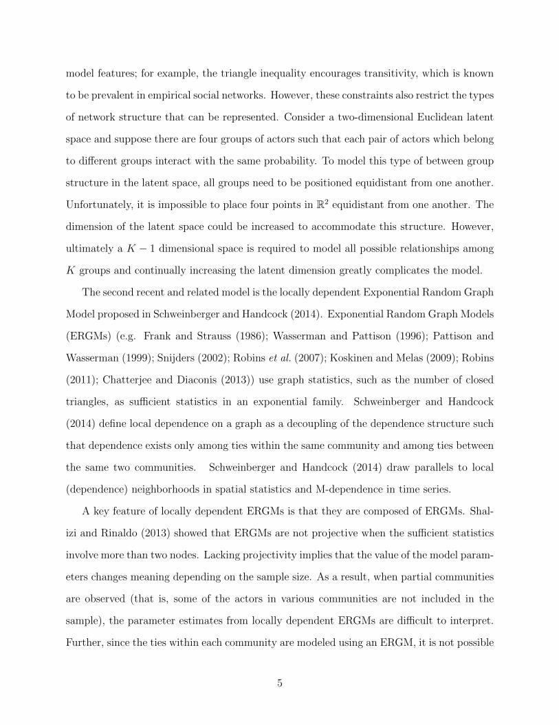
model features; for example, the triangle inequality encourages transitivity, which is known

to be prevalent in empirical social networks. However, these constraints also restrict the types

of network structure that can be represented. Consider a two-dimensional Euclidean latent

space and suppose there are four groups of actors such that each pair of actors which belong

to different groups interact with the same probability. To model this type of between group

structure in the latent space, all groups need to be positioned equidistant from one another.

Unfortunately, it is impossible to place four points in R2 equidistant from one another. The

dimension of the latent space could be increased to accommodate this structure. However,

ultimately a K − 1 dimensional space is required to model all possible relationships among

K groups and continually increasing the latent dimension greatly complicates the model.

The second recent and related model is the locally dependent Exponential Random Graph

Model proposed in Schweinberger and Handcock (2014). Exponential Random Graph Models

(ERGMs) (e.g. Frank and Strauss (1986); Wasserman and Pattison (1996); Pattison and

Wasserman (1999); Snijders (2002); Robins et al. (2007); Koskinen and Melas (2009); Robins

(2011); Chatterjee and Diaconis (2013)) use graph statistics, such as the number of closed

triangles, as sufficient statistics in an exponential family. Schweinberger and Handcock

(2014) define local dependence on a graph as a decoupling of the dependence structure such

that dependence exists only among ties within the same community and among ties between

the same two communities. Schweinberger and Handcock (2014) draw parallels to local

(dependence) neighborhoods in spatial statistics and M-dependence in time series.

A key feature of locally dependent ERGMs is that they are composed of ERGMs. Shal-

izi and Rinaldo (2013) showed that ERGMs are not projective when the sufficient statistics

involve more than two nodes. Lacking projectivity implies that the value of the model param-

eters changes meaning depending on the sample size. As a result, when partial communities

are observed (that is, some of the actors in various communities are not included in the

sample), the parameter estimates from locally dependent ERGMs are difficult to interpret.

Further, since the ties within each community are modeled using an ERGM, it is not possible

5

to compare parameters across communities within the same graph unless the communities

happen to be the same size. Locally dependent ERGMs are in fact projective if the sampling

units are taken to be communities rather than actors. Schweinberger and Handcock (2014)

calls this limited form of projectivity domain consistency. While our proposed model uses

a similar decomposition across subgraphs as Schweinberger and Handcock (2014), we model

within- and between-community structure using latent variable mixture models and show

the model class we define is projective when indexed by actors, broadening the notion of

local dependence and alleviating the challenges with interpretation and comparison.

2 Multiresolution network model

In this section, we propose a general modeling framework that reflects the global sparsity

and local density, “chain of islands” (Cross et al., 2001), structure observed in many large

networks.

Consider a hypothetical infinite population of actors and communities, where each actor

is a member of a single community. Define γ : N→ N to be the community membership map,

which partitions the actors into disjoint communities. That is, γ(i) = γi is the community of

actor i. Define KN = |γ({1, . . . , N})| to be the number of unique communities among actors

{1, ..., N}. The community map is only meaningful up to relabellings of the communities.

Without loss of generality we require that γi ≤ Ki−1 + 1 (defining K0 = 0) so that actors

1, . . . , N span communities 1, . . . , KN . In practice the community memberships are typically

estimated from the data, though in certain circumstances it can be defined a priori from

known structural breaks in the network (see Sweet et al. (2013) for an example).

Let Sk = {i : γi = k} be the collection of actors in community k in the population. We

assume that the number of actors in each community, e.g. |Sk|, is bounded, implying that

KN = O(N) as N →∞. Our assumption of bounded communities is supported by empirical

evidence that suggests the “best” communities contain small sets of actors, which are almost

6

disconnected from the rest of the network (Leskovec et al., 2009) and by psychologists and

primatologists who have proposed a limit on the size of human social networks (e.g. Dunbar

(1998)). This fact allows us to strategically allocate modeling effort within a large graph to

be concentrated on a relatively small portion of dyads. Since we postulate that the structure

of within-community relations will typically be most complex and interesting, we desire a

model flexible enough to differentially devote modeling effort to those relations.

Restricting community sizes to be bounded is also consistent with Schweinberger and

Handcock (2014), though their motivation is quite different. Following similar justification

as in the time series and spatial contexts, Schweinberger and Handcock (2014) define a

decomposition of the graph such that the propensity to form ties between any set of nodes

depends only on a finite number of other nodes. Along with global sparsity, the finite

communities assumption in Schweinberger and Handcock (2014) facilitates their asymptotic

normality results for graph statistics.

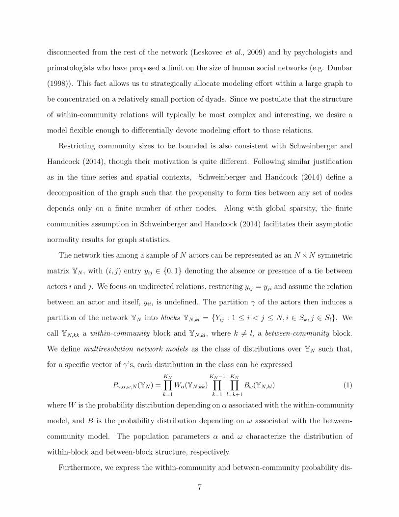
The network ties among a sample of N actors can be represented as an N×N symmetric

matrix YN , with (i, j) entry yij ∈ {0, 1} denoting the absence or presence of a tie between

actors i and j. We focus on undirected relations, restricting yij = yji and assume the relation

between an actor and itself, yii, is undefined. The partition γ of the actors then induces a

partition of the network YN into blocks YN,kl = {Yij : 1 ≤ i < j ≤ N, i ∈ Sk, j ∈ Sl}. We

call YN,kk a within-community block and YN,kl, where k 6= l, a between-community block.

We define multiresolution network models as the class of distributions over YN such that,

for a specific vector of γ’s, each distribution in the class can be expressed

Pγ,α,ω,N (YN ) =

KN∏k=1

Wα(YN,kk)KN−1∏k=1

KN∏l=k+1

Bω(YN,kl) (1)

whereW is the probability distribution depending on α associated with the within-community

model, and B is the probability distribution depending on ω associated with the between-

community model. The population parameters α and ω characterize the distribution of

within-block and between-block structure, respectively.

Furthermore, we express the within-community and between-community probability dis-

7

tributions as mixture distributions

Wα(YN,kk) =

∫W (YN,kk|ηk) dRα(ηk) (2)

Bω(YN,kl) =

∫B(YN,kl|τkl) dSω(τkl) (3)

and require the functional form of Bω(·) and Wα(·) do not depend on the size of the network,

N . Thus ηk is the within-community random effect for community k with random effect

distribution Rα and τkl is the between-community random effect for the pair of communities

k, l with distribution Sω. The dimension of both ηk and τkl do not depend on the sizes

of the respective blocks as they come from common distributions Rα and Sω. We assume

that both W and B are projective, which is in contrast to the Schweinberger and Handcock

(2014) strategy of assuming ERGMs as the between and within block distributions, which

are generally not projective. Projectivity of W and B is essential for coherent inference

based on the model; the importance of this property is detailed in Section 4.

In our probabilistic framework, we assume communities are exchangeable. That is, we

assume that the community labels can be arbitrarily permuted and the probability of the

network remains unchanged, or equivalently that there is no information about the social

structure of the network contained in the specific values of the community labels. We also

assume that the node labels within each community are exchangeable. A familiar case where

exchangeability does not hold is network data collected via snowball sampling, where nodes

are progressively sampled by following ties in the network and nodes close together in the

sampling order are likely to be connected.

We call the models in (1) multiresolution because the model parameters and random

effects correspond to parameters at three resolutions. At the coarsest (global) level, γ de-

fines the distribution of community sizes. Related literature on community detection defines

groups based on subgraph densities, such that actors have a higher propensity to interact

within the group than between groups (Newman, 2006), or based on stochastic equivalence,

8

where groups include actors that display similar interaction patterns to the rest of the net-

work (Lorrain and White, 1971). The most well-known models for community identification

is the stochastic block model (SBM) and its variants (Nowicki and Snijders, 2001; Airoldi et

al., 2008; Rohe et al., 2011; Choi et al., 2012; Amini et al., 2013). While these methods dis-

tinguish between clusters of actors and their aggregate structure at a macro-level, they lack

the ability to encode low-level structure such as transitivity, which manifests as triangles in

the network. Recent extensions of SBMs include “multiscale” versions (e.g. Peixoto (2014),

Lyzinski et al. (2015)), which repeatedly subdivide clusters. These models also fall within

our general class.

At the local level, α represents a (multivariate) population parameter determining the

distribution of within-community structure across the population, where we might expect

the richest structure. Recall the discussion in Section 1.1 about the LPCM and the inherent

constraints on the model tie propensities due to the latent space embedding. When multiple

dense pockets exist in a large, overall sparse network, the LPCM can sacrifice accuracy

in characterizing within cluster structure to distinguish between the clusters. Vivar and

Banks (2012) document a case involving baboon interactions where the separation of the

dense communities in a troop dominates the latent space positioning, crowding out within

group structure. Our model resolves this issue by disentangling the modeling of within

and between group relations. In particular, ω characterizes the distribution of between-

community relational structure across the population, and hence controls the overall sparsity

and small-world properties of the network.

While γ, α, and ω summarize global structure, at a finer resolution, ηk and τkl represent

the unique structure present within and between specific communities. Finally, at the finest

level of resolution, any actor-specific latent variables apart of each within-community distri-

bution W or each between-community relation distribution B provide local representations

of any involute structure. In the next section, we provide more concrete examples of these

parameters in the context of popular network models.

9

The general class of multiresolution models defined in (1) contains a diverse set of pos-

sible model specifications. The stochastic blockmodel (Holland et al., 1983), for example,

is a special case. The stochastic blockmodel decomposes a network into communities and

models the probability of a tie between any two actors as solely a function of their com-

munity memberships. In our formulation, ηk would denote the tie probability between two

individuals within community k and τkl would denote the tie probability between an actor

in community k and an actor in community l. Viewing these block-level probabilities as

random effects, Rα and Sω represent the mixing distribution governing the distributions of

these effects, and W and B represent products of independent and identically distributed

Bernoulli distributions. We could also construct a model that nests stochastic blockmodels

within one-another (Peixoto, 2014). With this approach, we would represent both within-

and between-community structure as a stochastic blockmodel. Greater nesting depths might

be specified for the within-community stochastic blockmodels to capture more complex pat-

terns within communities. Furthermore, separate random effects for sender and receiver

effects could be added to each block, as in the social relations model (Kenny and La Voie,

1984). In the following section, we explore another example of our model class, which we

call the Latent Space Stochastic Blockmodel.

3 Latent Space Stochastic Blockmodel

In this section, we introduce a particular multiresolution network model, called the Latent

Space Stochastic Blockmodel (LS-SBM). In the LS-SBM, the propensity for within-block

ties is modeled with a latent space model and the between-block ties are modeled as in a

stochastic blockmodel. We denote the probability an actor belongs to block k as πk, and let

π = (π1, ..., πKN ) denote the vector of membership probabilities, where∑KN

i=1 πi = 1.

The LS-SBM utilizes a latent Euclidean distance model (Hoff et al., 2002) for the within-

community distribution W . In this model the edges in YN,kk are conditionally independent

10

given the latent positions of the actors in Sk. Specifically, given Zi and Zj where i, j ∈

Sk, Yij is Bernoulli with probability logit−1(βk − ‖Zi − Zj‖), where ‖ · ‖ denotes the `2-

norm, i.e. Euclidean distance. The latent positions in group k are themselves independent

and identically distributed (IID) as spherically normal with mean zero and variance σ2k:

ND(Zi; 0, σ2kID). Thus

W (YN,kk|ηk) =

∫ (∏i,j

G(Yij; βk,Zi,Zj)

) (∏i

dND(Zi; 0, σ2kID)

), (4)

where G is the Bernoulli distribution stated above and the products are taken with respect

to all nodes in block k.

In the terminology of multiresolution models, ηk ≡ (βk, log σk) is the within-community

random effect governing the network structure within community k. βk can be interpreted as

the maximum logit-probability of a relation in block k: two nodes i and j are stochastically

equivalent in block k if and only if Zi = Zj, in which case P (Yij|Zi = Zj) = logit−1(βk). σk

is a measure of heterogeneity in block k, as σk = 0 is equivalent to an Erdos-Renyı model

with tie probability logit−1(βk). If σk = 0 for all blocks, then the multiresolution model

reduces to the stochastic blockmodel. We model ηk for all k = 1, . . . , KN as samples from a

bivariate normal with parameters α = {µ,Σ}. Thus, Rα(ηk) = N2((βk, log σk);µ,Σ).

For the between-community distribution B we use an Erdos-Renyı model. That is, all

edges between communities k and l are IID with probability τkl. Thus

B(YN,kl|τkl) =∏i∈Sk

∏j∈Sl

τYijkl (1− τkl)1−Yij . (5)

We model τkl as Beta distributed with parameters ω = (a0, b0): Sω(τkl) = Beta(τkl; a0, b0).

The model maintains a parsimonious structure in modeling relationships between blocks,

requiring only a single parameter, but is flexible in modeling ties within each block, allowing

tie prevalence to depend on the distance between actors in the unobserved social space.

There are two key differences between the proposed LS-SBM and the latent position

11

cluster model (LPCM) introduced in Handcock et al. (2007). The first key distinction is

that the probability of a tie between actors belonging to different communities in the LS-

SBM is a function of only their community memberships, whereas in the LPCM it is a

function of the distance between the actor positions in the latent space. This means that in

the LPCM, all of an actor’s ties and non-ties are used in determining the latent positions.

In contrast, in the LS-SBM, the latent space only affects within-community connections.

As a result, the structure of between-community connections are not constrained by the

dimension and geometry of the latent space in the LS-SBM like they are in the LPCM.

The second distinction between the models is that the LPCM contains a single intercept

parameter and the LS-SBM contains block-specific intercepts, βk. Each intercept βk can

be interpreted as the maximum logit-probability of a tie in community k. In practice, we

find there is often large heterogeneity in this maximum probability across communities,

suggesting having different intercepts is a critical piece of model flexibility in the LS-SBM.

3.1 Prior specification

Here we discuss the prior distributions for α and ω. Our intended application of the LS-SBM

is to networks where the within-community ties are denser than the between-community ties.

We use the prior on α to reflect this knowledge. Specifically, we set the prior on µ and Σ to be

a conjugate Normal-Inverse-Wishart distribution, with parameters {m0, s0,Ψ0, ν0}, subject

to an additional assortativity restriction. Given a0 and b0, the prior can be expressed

P (α|a0, b0,m0, s0,Ψ0, ν0) ∝N2(µ; m0,Σ0/s0)Inv.Wish(Σ; Ψ0, ν0)1(a0, b0,µ), (6)

where 1(a0, b0,µ) is the indicator function enforcing the assortativity condition. We fix a0

and b0 based on the observed density of the graph. The assortativity condition we require is

that the (logit) marginal probability of a within-community tie for the average block, induced

12

by µ, be larger than the (logit) average between-block probability of a tie, a0/(a0 + b0):

E[logit(Pr(Yij = 1))|γi = γj

]≥ E

[logit(Pr(Yij = 1))|γi 6= γj

]. (7)

Calculating these expectations (see the web-based supplementary materials for details), the

restriction on the population parameter space we wish to enforce is

µ1 − 2eµ2Γ(D+1

2)

Γ(D2

)≥ ψ(a0)− ψ(b0).

where ψ(x) is the digamma function defined ψ(x) = dlog(Γ(x))dx

. The digamma function is not

available in closed form but is easily approximated with most standard statistical software

packages. We proceed with estimation using this global assortativity restriction.

3.2 Estimation and block number selection

Here we provide a brief summary of our estimation procedure for the LS-SBM. A full descrip-

tion of the model specification and algorithm are provided in the web-based supplementary

materials. The posterior for our Bayesian model is not available in closed form, so instead we

approximate the posterior using draws obtained via Markov chain Monte Carlo (MCMC).

The MCMC algorithm performs the estimation with the number of blocks K fixed. Thus,

we first describe a procedure for choosing K and then outline the MCMC procedure given

the number of blocks.

We suggest comparing different K using a series of ten-fold cross-validation procedures.

For each repetition of the procedure, randomly partition the unordered node pairs into ten

folds. For each fold, use assortative spectral clustering (Saade et al., 2014) on the adjacency

matrix, excluding that fold, to partition the nodes into numbers of blocks K from 2 to

bN/4c. To adapt the spectral clustering algorithm to deal with the held out, missing at

random, edges we propose using an iterative EM-like scheme where first the missing values

are imputed using observed degrees, clustering is performed on the imputed data, and the

13

missing values from hold-out are re-imputed using the predicted probabilities. This should

be repeated, until convergence. This procedure does not require computing the full posterior

and can be done in parallel for each value of K and each validation fold.

For each repetition and K value, we propose calculating three metrics of predictive perfor-

mance: area under the ROC curve (AUC), mean squared error (MSE), and mean predictive

information (MPI). Calculate the mean value and 95% CIs for the mean of these criteria

over the repetitions for each K. Then, for each criteria, we suggest finding the smallest K

such that the mean value of the criteria for K falls in the 95% CI of the mean value of the

K with the best mean value (either maximal or minimal depending on the criterion).

Once we have selected a value of K, we use a Metropolis-within-Gibbs algorithm to ap-

proximate the joint posterior distribution. Our use of conjugate priors allows Gibbs updates

of π, τ ,µ, and Σ. We update each ηk with a Metropolis step, using a bivariate normal

proposal distribution.

Each node is assigned a single block membership at every iteration of the chain. This

block membership is jointly updated with the node’s latent position using a Metropolis step.

We also take additional (unsaved) Metropolis steps for the latent positions in order to allow

nodes which have switched blocks to find higher likelihood points in the latent space.

The likelihood is invariant to permutations of the block memberships and to rotations

and reflections of the latent spaces. We address these non-identifiabilities by post-processing

the posterior samples using equivalence classes defined over the parameter spaces. See the

supplementary materials for additional details.

In our experiments, computation was feasible for networks with three hundred nodes

in under two hours using a personal computer with a 2GHz processor and 8GB of RAM.

The most computationally expensive piece is the Metropolis step that jointly updates block

membership and latent positions and then subsequently takes additional draws from latent

spaces. In our experiments, however, using a joint update substantially improved mixing.

Since we do not use MCMC to compute K, this is not a limiting step computationally. To

14

scale our method beyond what is possible with MCMC, or for cases where the full posterior

is not of interest, we provide a two-stage fitting procedure in the supplementary material.

This procedure uses an assortative graph clustering algorithm to quickly estimate block

membership, and variational inference to estimate parameters within each block. We have

used this two-stage procedure to estimate our model in a sparse network with 13,000 nodes,

which took about three minutes on a standard personal computer. The results of this analysis

are provided in Section 3.3. Additional details about the two-stage procedure are provided

in the supplementary material.

3.3 Karnataka villages

We estimate the proposed LS-SBM on data from a social network study consisting of house-

holds in villages in Karnataka, India to illustrate the utility of the model. These data were

collected as part of an experiment to evaluate a micro-finance program performed by Baner-

jee et al. (2013). Data consist of multiple undirected relationships between individuals and

households in 75 villages. Relationship types include social and familial interactions (e.g.

being related or attending temple together) and views related to economic activity (e.g.

lending money or borrowing rice/ kerosene).

We used the household-level “visit” relation from village 59, which has N = 293 house-

holds with non-zero degree. We estimate the LS-SBM on the data with K = 6. Details of the

cross-validation selection procedure for K and LS-SBM estimation on this data are provided

in the supplementary materials. Codes to replicate the results we present here are available at

https://github.com/tedwestling/multiresolution_networks.git. Data are available

at https://dataverse.harvard.edu/dataset.xhtml?persistentId=hdl:1902.1/21538.

The results of the estimation algorithm are displayed in Figures 1, 2, and 3, and in Table

1. Figure 1 shows the observed adjacency matrix organized by marginal posterior mode block

membership. The estimated block memberships result in an assortative network structure:

there are more ties between households in the same community than between households

15

Figure 1: Household-level “visit” relation adjacency matrix of village number 59 from theKarnataka village dataset. Nodes are grouped by marginal posterior mode block member-ship.

Table 1: Between block probability matrix. The off-diagonal elements are the posteriormean probabilities of a tie between individuals in different blocks, τγiγj . The diagonal ele-ments represent the maximum probability of a tie within each block based on the block-levelparameter βk posterior mean: eβk/(1 + eβk). Values less than 0.01 are grayed out.

1 2 3 4 5 6

1 ≤.719 .006 .004 .044 .010 .0032 .006 ≤ .951 .018 .016 .006 .0033 .004 .018 ≤ .802 .011 .003 .0024 .044 .016 .011 ≤ .727 .079 .0215 .010 .006 .003 .079 ≤ .838 .0026 .003 .003 .002 .021 .002 ≤ .356

in different communities. Table 1 shows the posterior mean estimates of the between block

connectivity parameters, again illustrating the assortative patterns. The within-community

ties seen in Figure 1 are fairly clearly non-uniform, further justifying our departure from a

SBM for the within-community model.

Figure 2 shows the estimated block-level parameters ηk = (βk, log σk) and the global mean

µ = (µ1, µ2). Recall that βk is the intercept parameter for each block and log σk describes

the variation in the latent space. The µ1 and µ2 terms describe the mean of the distribution

of βk and log σk, respectively. Since the multiresolution framework is projective, we can

compare parameters between block-level parameters. Blocks two, five and six, denoted B2,

16

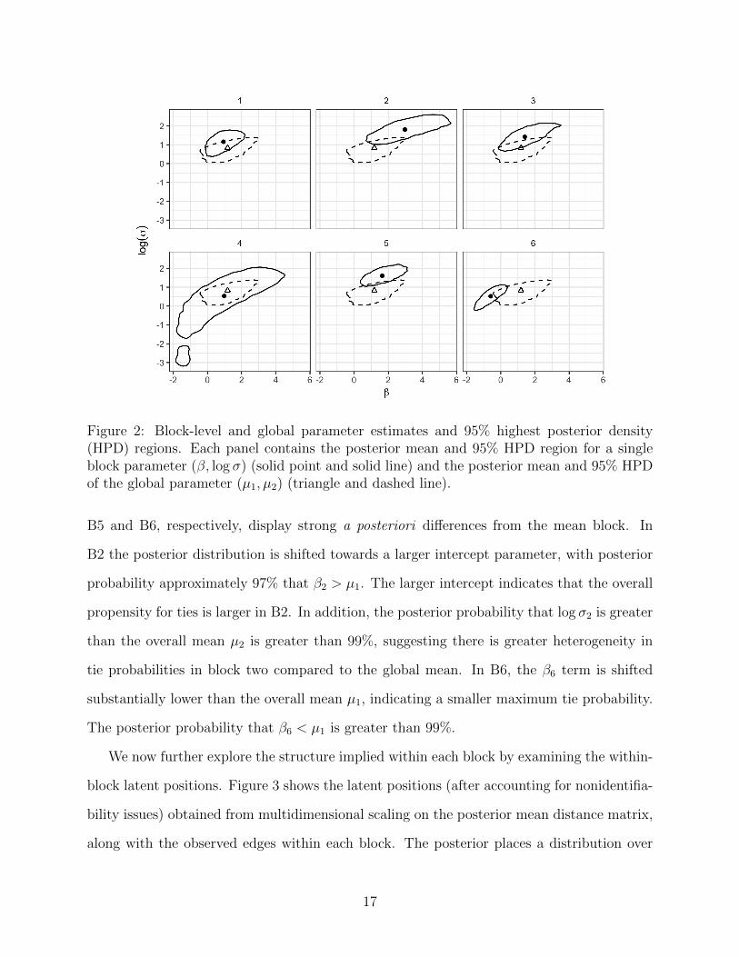
Figure 2: Block-level and global parameter estimates and 95% highest posterior density(HPD) regions. Each panel contains the posterior mean and 95% HPD region for a singleblock parameter (β, log σ) (solid point and solid line) and the posterior mean and 95% HPDof the global parameter (µ1, µ2) (triangle and dashed line).

B5 and B6, respectively, display strong a posteriori differences from the mean block. In

B2 the posterior distribution is shifted towards a larger intercept parameter, with posterior

probability approximately 97% that β2 > µ1. The larger intercept indicates that the overall

propensity for ties is larger in B2. In addition, the posterior probability that log σ2 is greater

than the overall mean µ2 is greater than 99%, suggesting there is greater heterogeneity in

tie probabilities in block two compared to the global mean. In B6, the β6 term is shifted

substantially lower than the overall mean µ1, indicating a smaller maximum tie probability.

The posterior probability that β6 < µ1 is greater than 99%.

We now further explore the structure implied within each block by examining the within-

block latent positions. Figure 3 shows the latent positions (after accounting for nonidentifia-

bility issues) obtained from multidimensional scaling on the posterior mean distance matrix,

along with the observed edges within each block. The posterior places a distribution over

17

Block 4 Block 5 Block 6

Block 1 Block 2 Block 3

−2 −1 0 1 2 3 −10 −5 0 5 10 −3 −2 −1 0 1 2 3

−5.0 −2.5 0.0 2.5 −5 0 5 10 −5 0 5

−5

0

5

10

−2

−1

0

1

2

3

−5

0

5

10

15

−10

−5

0

5

10

−5.0

−2.5

0.0

2.5

5.0

−3

−2

−1

0

1

2

Caste

General

Minority

OBC

Schedule caste

Schedule tribe

Figure 3: Latent positions within each block. Shading represents posterior probability ofinclusion in a given block, with the lightest shading representing a posterior estimate ofaround 30% and darkest colors representing values near unity. Colors and plot symbolsdifferentiate the five caste categories.

block memberships for each node, however in Figure 3 we show nodes only in the block for

which they have the largest posterior probability of inclusion. Individuals that are unlikely

to belong to any specific block (with inclusion probabilities less than 30%) are omitted.

Shading represents the concentration of the posterior over block memberships, with darker

colors indicating higher assignment probabilities.

Moving to the structure within the blocks, we investigate the relation between the house-

hold memberships, positions, and caste which is a formalized social class system in India.

Castes are denoted in Figure 3 using different colors. We see strong sorting by caste, with

almost all of the members of schedule castes and schedule tribes (the two lowest castes)

being grouped into B6. Members of the slightly higher class OBC (Other Backwards Caste)

are the most common in the network and are spread throughout the remaining blocks. An

extensive literature in economics (e.g. Townsend (1994); Munshi and Rosenzweig (2009);

Mazzocco (2012); Ambrus et al. (2014)) explores on the role of the caste system in individu-

18

als’ financial decisions. In particular this literature focuses on informal credit markets. That

is, the social structures that provide financial support in times of need without a formal, cor-

porate credit structure. Recent work by Ambrus et al. (2014) present a theoretical argument

for the importance of ties that bridge otherwise disconnected groups. In our results, these

individuals would be individuals whose block assignment based on their social interactions

does not match that of others in their caste. For example, this group of bridging individuals

would include members of schedule tribes or castes that are in blocks other than B6.

We also used our two-stage procedure (described in detail in the supplementary material)

to estimate our model for all 75 village networks combined. We formed an undirected network

of N = 13,009 nodes by combining all 75 household-level “visit” relation networks from the

Karnataka village data. We estimated the block structure using label propagation (Raghavan

et al., 2007), which returned 534 blocks. Every block contained only households from a single

village – that is, there were no blocks containing households from multiple villages. This

was expected since by design there are no between-village edges. There were a median of

six blocks per village, with as few as one block per village (i.e. the entire village constitutes

a single block) and as many as twenty blocks per village. The number of nodes per block

varied considerably, with a median of fourteen, mean of 24.4, and maximum of 233. The

density of edges within a block and nodes per block were well-described by a linear function

on the log-log scale with intercept 0.34 and slope -0.82, as shown in the left panel of Figure 4.

The estimated within-block latent space parameters log σ and β are shown in the right panel

of Figure 4. The larger blocks tend to be sparser and more heterogeneous, while the smaller

blocks are more homogeneous.

3.4 Simulation Study

In this section, we detail a simulation study illustrating the advantages of using a multires-

olution model like the LS-SBM over existing models such as the latent space model, LPCM

and SBM.

19

Figure 4: The left panel shows the log10 block density as a function of log10 block size.The blue line is the OLS linear regression fit. The right panel shows the block-level latentspace parameters βk and log(σk), where point size corresponds to block size and point colorcorresponds to block density. In both plots, each point is an estimated block from the modelfit to all 75 Karnataka villages using the two-stage procedure.

Binary, undirected network data were generated for 300 nodes from the LS-SBM model

with five equally-sized blocks such that the between-block tie probabilities were either 0.2 or

0.02. Within-block tie probabilities stemmed from a heterogeneous set of two-dimensional

block-specific latent spaces. Further details about the simulation parameters are provided in

the supplementary materials. One thousand simulations were performed where ten percent

of the undirected dyads in the network were held out in each simulation and the models were

fit to the remaining ninety percent of the data. Predictions were then made for the held out

portion of the network and the accuracy of these predictions quantified by computing the

area under the precision-recall curves. The results are shown in Figure 5.

20

Figure 5: Relative area under the precision-recall curve (AUPRC) based on out-of-sample predictions for the LS-SBM andthree existing models: latent space (LS) model, latent position cluster model (LPCM) and stochastic blockmodel (SBM). Theleftmost panel shows the relative AUPRC for all held out edges, the middle panel shows the results for edges that are betweennodes that are in different blocks and the right panel shows that for edges between nodes within the same block.

21

From the leftmost panel of Figure 5 it is evident the LS-SBM outperforms all three

existing models as the relative AUPRCs are greater than one for all simulations and all

network models. Separate precision-recall curves were constructed for the held out portions of

the network corresponding to relationships between nodes within the same block (rightmost

panel of Figure 5) and those portions between nodes that reside in different blocks (middle

panel of Figure 5). These illustrate that while the LS-SBM appears to predict edges between

nodes in different blocks as well as existing models, there are notable improvements in

predictions for ties between nodes within the same block.

4 Projectivity of multiresolution network models

Focusing on inference, we seek to understand which features of the hypothetical infinite

population we can reasonably expect to learn from a sample of N nodes. Projectivity is

essential for inference as it facilitates comparison of model parameters across networks of

different sizes. This notion of “different sizes” naturally arises in multiple network samples,

which are almost certainly never be of the same size (because of the complexities of sampling

networks and prevalence of missing data). In the case of the multiresolution framework, these

sizes may also refer to the inferred block sizes.

Shalizi and Rinaldo (2013) investigate the projectivity of families of statistical network

models, where a model family {Pθ,N : N ∈ N, θ ∈ Θ} is deemed projective if distribution

Pθ,N for a sample of N actors can be recovered by marginalizing the distribution Pθ,M , for

N < M , over actors {N + 1, . . . ,M}. Stated more formally, a family of network models is

projective if Pθ,N = Pθ,M ◦π−1M 7→N for all N < M <∞, where πM 7→N is the natural projection

map that selects the subgraph on the first N nodes from the full graph on M nodes and ◦

denotes function composition. Letting YM\N be YM after removing the YN subgraph and

22

YM\N be its sample space, we can write

Pθ,N(YN) = Pθ,M(π−1M 7→N(YN)) =

∑YM∈π−1

M 7→N (YN )

Pθ,M(YM) = Pθ,M(YN ,YM\N ∈ YM\N),

where π−1M 7→N(YN) is the set of graphs on {1, . . .M} that have YN as the subgraph on the

first N actors.

To see why projectivity is crucial for comparisons across networks of different sizes, or

equivalently blocks, recall the Karnataka dataset. Suppose we have a model family and

consider two village networks: village A network containing 100 households and village B

network containing 100, 000 households. Upon observing these networks, a researcher wishes

to formally compare them by fitting the statistical model to each one and comparing the

parameter estimates. In order for this comparison to be meaningful, the statistical model

must be projective. Suppose the parameter associated with the generation of network A

is θA, the parameter generating network B is θB, and θB = θA. The statistical model is

projective if, when 90,900 households are marginalized over in the network model fit to

network B, the resulting probability model on the remaining 100 households is equal to the

model on network A. (Note in this discussion, we assume the probability model is row and

column exchangeable, i.e. node exchangeable as in von Plato (1991).)

Our multiresolution framework proposes projective models, W and B, for capturing

within- and between-community relations, and combines these to form a model for the entire

network. We demonstrate below that a model class defined using combinations of projective

distributions forms a projective family of models. This permits researchers to make coherent

comparisons across communities within the same network, even if communities are of different

sizes.

We start by proving that mixtures of projective models are projective. In the definition of

multiresolution network models in (1)-(3), we assume that W and B are projective. Further,

since Wα and Bω are not indexed by N , Rα and Sω must be the same regardless of the number

23

of nodes in the graph. Below we show that this implies that Wα and Bω are projective by

showing that, in general, a mixture of projective models is also projective.

Theorem 1. Suppose {Pθ,M : M ∈ N, θ ∈ Θ} is a projective collection of statistical models

over networks and latent variables, such that Pθ,M is a distribution on (YM , η) supported

over YM ×N where the dimension of N does not depend on M . Let Pθ,M = Pθ,M ◦ τ−1M for

τM : YM ×N → YM the projection map. Then {Pθ,M : M ∈ N, θ ∈ Θ} is a projective family

as well.

Proof. Let N < M . Further, let πM 7→N be the projection map from YM ×N → YN ×N and

πM 7→N be the projection map from YM to YN . Let’s first suppose that

π−1M 7→N ◦ τ

−1N = τ−1

M ◦ π−1M 7→N . (8)

Then, Pθ,N = Pθ,N ◦τ−1N = Pθ,M ◦ π−1

M 7→N ◦τ−1N = Pθ,M ◦τ−1

M ◦π−1M 7→N = Pθ,M ◦π−1

M 7→N , where the

second equality follows from the projectivity of {Pθ,M : M ∈ N, θ ∈ Θ} and third equality is

a consequence of (8). Thus, if (8) holds, {Pθ,M : M ∈ N, θ ∈ Θ} is projective by definition.

Verifying (8) is straightforward. Let YN ∈ YN . Then

(π−1M 7→N ◦ τ

−1N

)(YN) = π−1

M 7→N

({(YN , η) :η∈N

})={(YN ,YM\N , η) :YM\N ∈YM\N , η∈N

}.

Similarly,

(τ−1M ◦ π

−1M 7→N

)(YN) = τ−1

M

({(YN ,YM\N) :YM\N ∈YM\N

})={(YN ,YM\N , η) :YM\N ∈YM\N , η∈N

}.

By a similar argument, we can show that node-level latent variable models, such as

the latent space network model specified for the within-block ties in the LS-SBM, are also

24

projective. Using Theorem 1, we now show that the class of multiresolution models is

projective.

Theorem 2. Multiresolution network models are projective.

Proof. Since W and B are projective models, the models Wα(YN,kk) and Bω(YN,kl) are

then projective by Theorem 1 because their distributions do not depend on N and they are

mixtures over projective models. Consider

Pγ,α,ω,M(YN ,YM\N ∈ YM\N) =

KM∏k=1

Wα(YN,kk,YM\N,kk ∈ YM\N,kk)

KM−1∏k=1

KM∏l=k+1

Bω(YN,kl,YM\N,kl ∈ YM\N,kl). (9)

For any k, l such that none of the nodes in blocks k, l are in YN , we have Wα(YN,kk,YM\N,kk ∈

YM\N,kk) = Wα(YM\N,kk ∈ YM\N,kk) = 1 and similarly for Bω. Hence we only need consider

blocks with at least one node from YN , and the right hand side of (9) is equal to

KN∏k=1

Wα(YN,kk,YM\N,kk ∈ YM\N,kk)KN−1∏k=1

KN∏l=k+1

Bω(YN,kl,YM\N,kl ∈ YM\N,kl).

Since Wα and Bω are projective, Wα(YN,kk,YM\N,kk ∈ YM\N,kk) = Wα(YN,kk), and similarly

for Bω. Thus the right hand side of (9) is equal to

KN∏k=1

Wα(YN,kk)

KN−1∏k=1

KN∏l=k+1

Bω(YN,kl),

which equals Pγ,α,ω,N(YN).

We emphasize that projectivity of the multiresolution model only occurs when Bω and

Wα are both projective, and hence these distributions do not depend on N . If the between-

block tie probabilities depend on the size of the observed graph, then the model is not

projective overall but is projective within each block. By “projective within each block” we

25

mean that the within-block parameters are still comparable across blocks and networks of

different sizes, although it is meaningless to, in general, compare the between-block param-

eters. An advantage of the between-block parameters depending on N is that the model

can be sparse in the limit. That is, as the number of nodes grows from N to infinity, the

expected density (i.e. proportion of edges present in the graph) goes to zero. Equivalently,

a graph is asymptotically sparse if the average expected degree grows sub-linearly with N .

The Aldous-Hoover Theorem implies that infinitely exchangeable sequences of nodes corre-

spond to dense graphs (Aldous, 1981; Orbanz and Roy, 2015). In our case, however, for

a fixed N and γ, the multiresolution model is only exchangeable modulo γ, meaning that

nodes within the same block are exchangeable (similar to that in regression; see McCullagh

(2005)). If we assume each node has an equal probability of belonging to any block (e.g.

placing a uniform distribution on each γi), the model is finitely exchangeable (von Plato,

1991). However, we are unaware of a prior distribution on γ that gives both finite exchange-

ability and projectivity, but does not assume knowledge about a bound on the size of blocks.

In the web-based supplementary material we show that families of projective models which

are finitely exchangeable are asymptotically dense. Nevertheless, for practical purposes, our

model can be arbitrarily sparse for any network with a finite number of nodes and, since it

is projective, permit comparison between networks of different sizes.

Our results on exchangeability and projectivity relate to recent work on nonparametric

generative models for networks (e.g. Caron and Fox (2014), Veitch and Roy (2015), Crane and

Dempsey (2015), Crane and Dempsey (2016), or Broderick and Cai (2016)). The objectives

in our framework are subtly but critically different, however. In recent developments in

nonparametrics, the objective is to understand the structure of the graph that is implied by

a probability model as the network grows from the observed size N to its limit. These recent

works define new notions of exchangeability that imply critically different graph properties

than node exchangeability discussed here. Our work, in contrast, focuses on the inverse

inference paradigm: given a sample from an infinite population, our goal is to understand

26

which properties of the population could be feasibly estimated using the multiresolution

model. This perspective leads to a focus on projectivity.

5 Discussion

In this paper we present a multiresolution model for social network data. Our model is

well-suited for graphs that are overall very sparse, but contain pockets of local density.

Our model utilizes mixtures of projective models to separately characterize tie structure

within and between dense pockets in the graph. Our proposed framework is substantially

more flexible than existing latent variable approaches (such as the LPCM) and supports

meaningful comparisons of parameter estimates across communities and networks of varying

sizes.

We introduced the LS-SBM as one example of a model within the multiresolution class.

However, alternative multiresolution models could be defined by replacing the latent space

model representing within-community relations with LPCMs or LS-SBMs. This would add

complexity to the model, allowing for sub-community structure within the global-community

structure. A key distinction between the general multiresolution framework propose here and

previous approaches of, for example, Peixoto and Lyzinski et al. is that our approach allows

and suggests using different network models to capture structure at different levels. This

allows models to be constructed that leverage the advantages (e.g. parsimony, detailed

structure) of multiple models simultaneously.

Our work also contributes to an active discussion in the statistics literature emphasizing

the importance of understanding the relationship between sampling and modeling social

networks. Crane and Dempsey (2015), for example, present a general framework for sampling

and inference for network models. Our work emphasizes the importance of “consistency

under sampling” for comparison across networks and across communities within the same

graph.

27

Our projectivity result for multiresolution models means that our framework can be used

to compare across communities within a graph, even if the communities are different sizes.

Schweinberger and Handcock (2014) define the concept of domain consistency, which can

be thought of as projectivity over communities, and propose a class of models that satisfy

this property. If, for example, a member of a community is missing, then the interpretation

of the parameters describing behavior in that community will be fundamentally different

than if the member were present. Our model also has this property, but is more general.

In particular, the notion of projectivity over communities requires that data be collected

by using cluster sampling over communities. Here we strengthened and generalized this

framework by proving that our model is projective at the actor level, i.e. even if complete

communities are not observed. Using our framework, it is possible to sample at the actor

rather than the community level while estimating parameters that are comparable across

communities.

Acknowledgements This work was partially supported by the National Science Foun-

dation under Grant Number SES-1461495 to Fosdick and Grant Number SES-1559778 to

McCormick. McCormick is also supported by grant number K01 HD078452 from the Na-

tional Institute of Child Health and Human Development (NICHD). This material is based

upon work supported by, or in part by, the U. S. Army Research Laboratory and the

U. S. Army Research Office under contract/grant number W911NF-12-1-0379. Murphy

and Ng are supported by the Science Foundation Ireland funded Insight Research Centre

(SFI/12/RC/2289). The authors would also like to thank the Isaac Newton Institute Pro-

gram on Theoretical Foundations for Statistical Network Analysis workshop on Bayesian

Models for Networks, supported by EPSRC grant number EP/K032208/1.

28

References

E. M. Airoldi, D. M. Blei, S. E. Fienberg, and E. P. Xing. Mixed membership stochastic

blockmodels. Journal of Machine Learning Research, 9:1981–2014, 2008.

D. J. Aldous. Representations for partially exchangeable arrays of random variables. Journal

of Multivariate Analysis, 11(4):581–598, 1981.

A. Ambrus, A. G. Chandrasekhar, and M. Elliott. Social investments, informal risk sharing,

and inequality. Technical report, National Bureau of Economic Research, 2014.

A. A. Amini, A. Chen, P. J. Bickel, and E. Levina. Pseudo-likelihood methods for community

detection in large sparse networks. The Annals of Statistics, 41(4):2097–2122, 2013.

A. Banerjee, A. G. Chandrasekhar, E. Duflo, and M. O. Jackson. The diffusion of microfi-

nance. Science, 341(6144):1236498, 2013.

S. P. Borgatti, A. Mehra, D. J. Brass, and G. Labianca. Network analysis in the social

sciences. Science, 323(5916):892–895, 2009.

T. Broderick and D. Cai. Edge-exchangeable graphs and sparsity. arXiv preprint

arXiv:1603.06898, 2016.

F. Caron and E. B. Fox. Sparse graphs using exchangeable random measures. arXiv preprint

arXiv:1401.1137, 2014.

B. Carpenter, A. Gelman, M. Hoffman, D. Lee, B. Goodrich, M. Betancourt, M. A. Brubaker,

J. Guo, P. Li, and A. Riddell. Stan: A probabilistic programming language. Journal of

Statistical Software, 2016.

S. Chatterjee and P. Diaconis. Estimating and understanding exponential random graph

models. The Annals of Statistics, 41(5):2428–2461, 2013.

29

D. S. Choi, P. J. Wolfe, and E. M. Airoldi. Stochastic blockmodels with a growing number

of classes. Biometrika, 99(2):273–284, 2012.

H. Crane and W. Dempsey. A framework for statistical network modeling. arXiv preprint

arXiv:1509.08185, 2015.

H. Crane and W. Dempsey. Edge exchangeable models for network data. arXiv preprint

arXiv:1603.04571, 2016.

R. Cross, A. Parker, L. Prusak, and S. P. Borgatti. Knowing what we know. Organizational

Dynamics, 30(2):100–120, 2001.

J. de Leeuw and P. Mair. Multidimensional scaling using majorization: SMACOF in R.

Journal of Statistical Software, 31(i03), 2009.

R. Dunbar. The social brain hypothesis. Brain, 9(10):178–190, 1998.

C. Fraley and A. E. Raftery. Model-based clustering, discriminant analysis, and density

estimation. Journal of the American Statistical Association, 97(458):611–631, 2002.

O. Frank and D. Strauss. Markov graphs. Journal of the American Statistical Association,

81(395):832–842, 1986.

A. Gelman, J. B. Carlin, H. S. Stern, and D. B. Rubin. Bayesian data analysis, volume 2.

Chapman & Hall/CRC Boca Raton, FL, USA, 2014.

M. S. Handcock, A. E. Raftery, and J. M. Tantrum. Model-based clustering for social net-

works. Journal of the Royal Statistical Society: Series A (Statistics in Society), 170(2):301–

354, 2007.

P. D. Hoff, A. E. Raftery, and M. S. Handcock. Latent space approaches to social network

analysis. Journal of the American Statistical Association, 97:1090–1098, 2002.

30

P. W. Holland, K. B. Laskey, and S. Leinhardt. Stochastic blockmodels: First steps. Social

Networks, 5(2):109–137, 1983.

C. H. Jackson. Multi-state models for panel data: The msm package for R. Journal of

Statistical Software, 38(8):1–29, 2011.

A. Jasra, C. C. Holmes, and D. A. Stephens. Markov chain Monte Carlo methods and the

label switching problem in Bayesian mixture modeling. Statistical Science, 20(1):50–67,

02 2005.

D. A. Kenny and L. La Voie. The social relations model. Advances in Experimental Social

Psychology, 18:141–182, 1984.

J. Koskinen and V. Melas. Using latent variables to account for heterogeneity in exponential

family random graph models. In S. M. Ermakov, V. B. Melas, and A. N. Pepelyshev,

editors, Proceedings of the 6th St. Petersburg Workshop on Simulation, pages 845–849. St

Petersburg State University, 2009.

J. Leskovec, K. J. Lang, A. Dasgupta, and M. W. Mahoney. Community structure in large

networks: Natural cluster sizes and the absence of large well-defined clusters. Internet

Mathematics, 6(1):29–123, 2009.

F. Lorrain and H. C. White. Structural equivalence of individuals in social networks. The

Journal of Mathematical Sociology, 1(1):49–80, 1971.

V. Lyzinski, M. Tang, A. Athreya, Y. Park, and C. E. Priebe. Community detection and

classification in hierarchical stochastic blockmodels. arXiv preprint arXiv:1503.02115,

2015.

M. Mazzocco. Testing efficient risk sharing with heterogeneous risk preferences. The Amer-

ican Economic Review, 102(1):428–468, 2012.

31

P. McCullagh. Exchangeability and regression models. Oxford Statistical Science Series,

33:89, 2005.

K. Munshi and M. Rosenzweig. Why is mobility in India so low? Social insurance, inequality,

and growth. Technical report, National Bureau of Economic Research, 2009.

M. E. Newman. Modularity and community structure in networks. Proceedings of the

National Academy of Sciences, 103(23):8577–8582, 2006.

K. Nowicki and T. A. B. Snijders. Estimation and prediction for stochastic blockstructures.

Journal of the American Statistical Association, 96(455):1077–1087, 2001.

P. Orbanz and D. M. Roy. Bayesian models of graphs, arrays and other exchangeable random

structures. IEEE Transactions on Pattern Analysis and Machine Intelligence, 37(2):437–

461, 2015.

G. L. Page and F. A. Quintana. Spatial product partition models. Bayesian Analysis,

11(1):265–298, 2016.

C. H. Papadimitriou and K. Steiglitz. Combinatorial optimization: Algorithms and complex-

ity. Courier Corporation, 1998.

P. Pattison and S. Wasserman. Logit models and logistic regressions for social networks:

II. Multivariate relations. British Journal of Mathematical and Statistical Psychology,

52(2):169–193, 1999.

T. P. Peixoto. Hierarchical block structures and high-resolution model selection in large

networks. Physical Review X, 4(1):011047, 2014.

U. N. Raghavan, R. Albert, and S. Kumara. Near linear time algorithm to detect community

structures in large-scale networks. Physical review E, 76(3):036106, 2007.

G. Robins, P. Pattison, Y. Kalish, and D. Lusher. An introduction to exponential random

graph (p*) models for social networks. Social Networks, 29(2):173–191, 2007.

32

G. Robins. Exponential random graph models for social networks. Encyclopaedia of Com-

plexity and System Science, Springer, 2011.

C. E. Rodrıguez and S. G. Walker. Label switching in Bayesian mixture models: Determin-

istic relabeling strategies. Journal of Computational and Graphical Statistics, 23(1):25–45,

2014.

G. Rodriguez-Yam, R. A. Davis, and L. L. Scharf. Efficient Gibbs sampling of truncated mul-

tivariate normal with application to constrained linear regression. Unpublished manuscript,

2004.

K. Rohe, S. Chatterjee, B. Yu, et al. Spectral clustering and the high-dimensional stochastic

blockmodel. The Annals of Statistics, 39(4):1878–1915, 2011.

A. Saade, F. Krzakala, and L. Zdeborova. Spectral clustering of graphs with the Bethe

Hessian. In Advances in Neural Information Processing Systems, pages 406–414, 2014.

M. Salter-Townshend and T. B. Murphy. Variational Bayesian inference for the latent posi-

tion cluster model for network data. Computational Statistics & Data Analysis, 57(1):661–

671, 2013.

M. Salter-Townshend, A. White, I. Gollini, and T. B. Murphy. Review of statistical net-

work analysis: Models, algorithms, and software. Statistical Analysis and Data Mining,

5(4):243–264, 2012.

M. Salter-Townshend. Package VBLPCM, 2015.

M. Schweinberger and M. S. Handcock. Local dependence in random graph models: Char-

acterization, properties and statistical inference. Journal of the Royal Statistical Society:

Series B, 2014.

C. R. Shalizi and A. Rinaldo. Consistency under sampling of exponential random graph

models. The Annals of Statistics, 41(2):508–535, 2013.

33

T. A. Snijders. Markov chain Monte Carlo estimation of exponential random graph models.

Journal of Social Structure, 3(2):1–40, 2002.

T. M. Sweet, A. C. Thomas, and B. W. Junker. Hierarchical network models for education

research hierarchical latent space models. Journal of Educational and Behavioral Statistics,

38(3):295–318, 2013.

R. M. Townsend. Risk and insurance in village India. Econometrica: Journal of the Econo-

metric Society, pages 539–591, 1994.

J. Ugander, B. Karrer, L. Backstrom, and C. Marlow. The anatomy of the Facebook social

graph. arXiv preprint arXiv:1111.4503, 2011.

V. Veitch and D. M. Roy. The class of random graphs arising from exchangeable random

measures. arXiv preprint arXiv:1512.03099, 2015.

J. C. Vivar and D. Banks. Models for networks: A cross-disciplinary science. Wiley Inter-

disciplinary Reviews: Computational Statistics, 4(1):13–27, 2012.

J. von Plato. Finite partial exchangeability. Statistics & Probability Letters, 11(2):99–102,

1991.

S. Wasserman and P. Pattison. Logit models and logistic regressions for social networks: I.

An introduction to Markov graphs and p*. Psychometrika, 61(3):401–425, 1996.

34

Web-based supplementary materials

A Interplay between finite exchangeability, projectiv-

ity, and asymptotic sparsity

The relationship between (finite) exchangeability and projectivity is an important part of our

modeling framework. Since we restrict the size of each community to be finite, our model is

finitely exchangeable (and not infinitely exchangeable). We now show that, even with finite

exchangeabiltiy, a model that is projective is also dense in the limit.

Theorem 3. Projective families of finitely node-exchangeable models for networks are asymp-

totically dense.

Proof. First we write

EPN,θ

[∑YN

Yij

]=∑YN

PN,θ(Yij = 1).

Now we can write the marginal probability as

PN,θ(Yij = 1) = PN,θ(Y12) = PN,θ(Y12 = 1,YN\12 ∈ YN\12) = P2,θ(Y12)

where the first equality was by exchangeability of the distribution PN,θ and the second two

by projectivity. Hence the probabilities in the sum are all the same and the expected number

of edges in the newtork is

EPN,θ

[∑YN

Yij

]= 1

2N(N − 1)P2,θ(Y12).

Hence the family is asymptotically dense with asymptotic density P2,θ(Y12).

35

B Prior specification in the LS-SBM

The assortativity restriction discussed in Section 3.1 and shown in (7) required the mean

(logit) probability of a tie within blocks be greater than or equal to the mean (logit) proba-

bility of a tie between blocks. To translate this restriction into constraints on the parameters,

first consider the within-block tie probabilities. It can be shown

E[‖Zi − Zj‖

]= 2σk

Γ(D+12

)

Γ(D2

).

Then, if Z1, ...,ZN are IID ND(0, σ2kID), where D is the dimension of the latent space, the

conditional expected logit is equal to

E[logit(Pr(Yij = 1))|γi = γj = k, βk, σk

]= βk − 2σk

Γ(D+12

)

Γ(D2

).

Taking expectations then over the distribution of ηk = (βk, σk), we find

E[logit(Pr(Yij = 1))|γi = γj

]= µ1 − 2eµ2

Γ(D+12

)

Γ(D2

). (10)

Recall the between block tie probabilities Pr(Yij = 1|γi 6= γj, τγiγj) = τγiγj . Then for γi 6= γj,

logit(Pr(Yij = 1)) = log(

τγiγj1−τγiγj

)and marginalizing over the Beta distribution, we find

E[logit(Pr(Yij = 1))|γi 6= γj

]= ψ(a0)− ψ(b0), (11)

where ψ(x) is the digamma function: ψ(x) = dlog(Γ(x))dx

.

Combining equations (10) and (11), the restriction on the population parameter space is

µ1 − 2eµ2Γ(D+1

2)

Γ(D2

)≥ ψ(a0)− ψ(b0).

This constraint is incorporated in the prior specification in (6) in the manuscript.

36

C Steps for choosing number of blocks

We now detail our method of pre-selecting the number of blocks K for a network using cross-

validated spectral clustering. Let Kmax be the maximal number of clusters the researcher

wants to consider.

Let A = {(i, j) : 1 ≤ i < j ≤ N} be the set of possible edges in an undirected binary

network with no self-loops.

1. Create a square matrix Pk of the same dimensions as the observed network Y for each

k = 1, . . . , Kmax. P will contain the held-out predicted probabilities for probabilties.

2. Randomly partition A in to MCV folds of equal size A1, . . . ,AMCV(or as close to equal

size as possible).

3. For m = 1, . . . ,MCV :

(a) Create a network Y (m) which is a copy of the observed network Y except that

Y(m)i,j is missing for all (i, j) ∈ Am.

(b) Impute the elements of Am in Y (m) using the observed degrees of each node

(i.e. Y(m)i,j = didj where di is the fraction of observed edges among non-missing

possibilities for node i).

(c) For each k = 1, . . . , Kmax:

i. Estimate a degree-corrected stochastic block model on Y (m) with k blocks

using, e.g. assortative spectral clustering.

ii. Re-impute the elements of Am in Y (m) using the predicted probabilities from

the estimated degree corrected stochastic block model.

iii. Repeat until the sum of the squared differences in predicted probabilities from

one iteration to the next falls below a desired threshold.

iv. Set the elements of Am in Pk to be the predicted probabilities from the final

stochastic block model fit.

37

4. Calculate the AUC, MSE, and MPI between Pk and Y for each k.

We repeated the above procedure twenty times (with different random folds each time) to

obtain ten out-of-sample AUC, MSE, and MPI estimates for each possible K. We then

computed the mean AUC, MSE, and MPI and a 95% confidence interval for this mean for

each K. Each measure had a value of K that minimized the measure – for each measure we

defined the selected number of blocks based on that measure as the smallest K whose 95%

confidence interval contained the mean of the optimal K.

D LPCM on Karnataka village dataset

As a comparison, we also present the fit from the LPCM in Figure 6. We fit the LPCM

using the variational approximation of Salter-Townshend and Murphy (2013) provided in

the R package ‘VBLPCM’ (Salter-Townshend, 2015). We used six clusters in the LPCM

for comparison with our six blocks. A first key distinction is that the LPCM has a smaller

global intercept term than µ1 and is forced to capture heterogeneity in tie propensity by

expanding the distance between clusters (and thereby individuals) in the latent space. This

approach is in contrast to the LS-SBM which maintains block specific intercepts and latent

spaces, facilitating comparison across blocks. Consequences of encoding all clusters in the

same latent space is that tie propensities are extremely small between groups on opposite

sides of the latent space and relations between groups that are adjacent are constrained by

the triangle inequality. The group represented in green, for example, is adjacent to the group

in pink, but by virtue of the distance between the pink and teal groups, must also be close

to the group in teal.

38

−5 0 5

−8−6

−4−2

02

46

Latent Position Cluster Model

First latent dimension

Seco

nd la

tent

dim

ensi

on

Posterior mode of β0=.003

Figure 6: LPCM latent positions for the household-level “visit” relation data for villagenumber 59 from the Karnataka village dataset.

E Sampling algorithm

In this section, we give the details of the sampling algorithm. For priors we set

γi ∼ Categorical(π) i = 1, ..., N

π ∼ Dirichlet(υ0, . . . , υ0)

τ kl ∼ Beta(a0, b0) 1 ≤ k < l ≤ N

(µ|Σ) ∼ MVN(m0, s−10 Σ)

Σ ∼ InvWishart(Ψ0, ν0).

39

Denote the full set of parameters ζ = {γ, τ ,Z, β, π, σ, µ,Σ}. Also define αk = (βk, log σk)

as the within-block latent space parameters. The posterior factors as

P (ζ|Y ) ∝ P (Y |γ, τ ,Z, β)P (γ|π)P (Z|σ)P (β,σ, τ |µ,Σ, a0, b0)

× P (π|υ0)P (µ|Σ,m0, s0)P (Σ|Ψ0, ν0),

The full posterior is not available in closed form. We thus take draws from the posterior

using the Markov chain Monte Carlo algorithm below (all parameters besides the one being

updated are understood be set to their latest values).

Let nk =∑

i 1γi=k denote the number of nodes in block k, α(t) = 1K

∑kα

(t)k be the sample

mean of the block-level α parameters, and S(t)α =

∑k

(α

(t)k − α(t)

)(α

(t)k − α(t)

)T. Given an

admissible set of initialization values, iteration t + 1 of the sampling algorithm proceeds as

follows:

1. For i = 1, 2, . . . , N :

(a) Propose γ∗i ∼ Categorical(λ(t)i1 /Σkλ

(t)ik , ...., λ

(t)iK/Σkλ

(t)ik ) where

λik =ε+

∑j∈Sk Yij

|Sk|+ 1

In words, the probability that the proposal for node i is block k is proportional

to the number of ties i has to the block plus ε divided by the size of the block

plus one. The presence of ε avoids probabilities equal to 0 or 1 and encourages

jumping to blocks with few nodes.

(b) Conditional on this configuration of group memberships, propose Z∗i |γ∗i ∼ MVND(m∗i , r2ZID),

40

where

m∗i =

Z(t)i , γ∗i = γ

(t)i

1

|G(t)i,γ∗i|

∑j∈G(t)

i,γ∗i

Z(t)j , γ∗i 6= γ

(t)i and |G(t)

i,γ∗i| > 0

0, otherwise.

Here G(t)i,γ∗i

= {j : γ(t)j = γ∗i , Yij = 1} is the set of nodes in the same proposed block

as i to which i is connected. In words, if i stays in the same block, center at its

last position. If it moves to a new block and has ties in that block, center at the

mean position of its ties in that block. If it moves to a new block and does not

have any ties in that block, center at the origin. The variance of the proposed

position coordinates equals r2Z .

(c) Set (γ(t+1)i ,Z

(t+1)i ) = (γ∗i ,Z

∗i ) with probability

p(γ∗i ,Z∗i |others)q(γ

(t)i ,Z

(t)i |γ∗i ,Z∗i )

p(γ(t)i ,Z

(t)i |others)q(γ∗i ,Z

∗i |γ

(t)i ,Z

(t)i )

where q((1)|(2)) is shorthand for the transition density to (1) from (2). For the

first ratio we have

p(γ∗i ,Z∗i |others)

p(γ(t)i ,Z

(t)i |others)

=p(Y |γ∗,Z∗, τ (t),β(t))p(γ∗i |π(t))p(Z∗i |σ(t))

p(Y |γ(t),Z(t), τ (t),β(t))p(γ(t)i |π(t))p(Z

(t)i |σ(t))

.

For the second ratio, we have

q(γ∗i ,Z∗i |γ

(t)i ,Z

(t)i ) = q(γ∗i |γ

(t)i )q(Z∗i |γ∗i , γ

(t)i ,Z

(t)i )

=

[∏j

(λ(t)ij /Σkλ

(t)ik )1{γ

∗i =j}

]φD(Z∗i ; m

∗i (γ∗i ,γ

(t),Z(t)), r2ZID

)and analogously for the numerator.

2. For each i = 1, . . . , N propose Z∗i ∼ MVND(Z(t)i , r

2ZID), and set Z

(t+1)i = Z∗i with

41

probability [∏j∈Sk p(Yij|Z

∗i ,Zj,βk)

]φD(Z∗i ; 0, σ2

kID)[∏j∈Sk p(Yij|Z

(t)i ,Zj,βk)

]φD(Z

(t)i ; 0, σ2

kID)

where here k = γi. Otherwise Z(t+1)i = Z

(t)i . This step updates the latent positions of

each node, without updating the block memberships.

3. Sample π(t+1) ∼ Dirichlet(υ0 + n(t)1 , . . . , υ0 + n

(t)K ).

4. For k = 2, . . . , K and l = 1, . . . , k − 1, sample τ ∗kl ∼ Beta(a0kl + skl, b0kl + nknl − skl),

where skl =∑

i,j Yij1γi=k,γj=l is the number of edges between blocks k and l. Set

τ(t+1)kl = τ ∗kl.

5. For k = 1, . . . , K, let αk = (βk, log(σk)) and sample α∗k ∼ MVN2(α(t)k , Aα). Set

α(t+1)k = α∗k with probability

[∏i,j∈Sk P (Yij|Zi,Zj, β

∗k)]∏

i∈Sk [φD(Zi; 0, σ2∗k ID)][∏

i,j∈Sk P (Yij|Zi,Zj, β(t)k )]∏

i∈Sk

[φD(Zi; 0, σ

2(t)k ID)

]φD(α∗k;µ,Σ)

φD(α(t)k ;µ,Σ)

.

6. Sample each component of µ = (µ1, µ2) one at a time from their respective full condi-

tional distribution given all other parameters and subject to the assortativity restric-

tion. More details given below.

7. Sample

Σ(t+1) ∼ InvWishart(Ψ0 + S(t)

α + Ks0K+s0

(α(t) −m0

)(α(t) −m0

)T, K + ν0

).

The above algorithm is repeated numerous times until a suitable sample from the posterior

distribution is obtained.

42

We now describe the process of sampling from the vector of global within-community

means, µ. First note that without restricting assortativity, the (joint) full conditional is:

µ(t+1) ∼ MVN

(m =

Kα(t) + s0m0

K + s0

, Σ = (K + s0)−1Σ(t)

).

Denote the components of m = (m1, m2) and the components of Σ as σ21, σ2

2, and ρ. Recall

that our restriction for assortativity is:

E[logit(Pr(Yij = 1))|γi = γj

]≥ E

[logit(Pr(Yij = 1))|γi 6= γj

].

Given this restriction, the full conditional for µ becomes truncated multivariate normal.

While efficient algorithms exist for sampling from truncated multivariate normals subject to

linear constraints (e.g. Rodriguez-Yam et al. (2004) and others), the logit function means

that our constraints on the parameters space are nonlinear. Thus, instead of sampling from

the multivariate normal, we update each component of µ conditional on the others.

The assortativity constraint can be expressed in terms of µ as

µ1 − 2eµ2Γ(D+1

2)

Γ(D2

)≥ ψ(a0)− ψ(b0).

Updating µ thus involves two steps:

1. Update µ(t+1)1 subject to

µ(t+1)1 ≥ f1(a0, b0, µ

(t)2 ) ≡ ψ(a0)− ψ(b0)− 2eµ

(t)2

Γ(D+12

)

Γ(D2

)

by drawing from the truncated normal

µ(t+1)1 ∼ N

(m1 +

σ1

σ2

ρ(µ

(t)2 − m2

),(1− ρ2

)σ2

1

)1(µ1 ≥ f1(a0, b0, µ

(t)2 ))

43

2. Update µ(t+1)2 subject to

µ(t+1)2 ≤ f2(a0, b0, µ

(t)1 ) ≡ log

(−

Γ(D2

)

2Γ(D+12

)

(ψ(a0)− ψ(b0)− µ(t)

1

))

by drawing from the truncated normal

µ(t+1)2 ∼ N

(m2 +

σ2

σ1

ρ(µ

(t)1 − m1

),(1− ρ2

)σ2

2

)1(µ2 ≤ f2(a0, b0, µ

(t)1 )).

We obtained truncated normal draws using the rtnorm function in the msm package (Jackson

(2011)).

F Sampler post-processing

The likelihood is invariant to permutations of the block memberships and to rotations and

reflections of the latent spaces. We post-process the MCMC samples to resolve these non-

identifiabilities.

The invariance of the likelihood to permutations of the block memberships is called label-

switching and it has been studied extensively (eg. Jasra et al., 2005; Rodrıguez and Walker,

2014). In order to handle the label-switching invariance of the block memberships, we first

fix a membership vector γ0 = (γ01 , ....γ

0N) toward which to permute the memberships. While

multiple choices for γ0 are possible, we use a random membership vector from one of the

chains. For each membership sample γs = (γ(s)1 , ..., γ

(s)N ) we use the Hungarian algorithm

to find a permutation ω of 1, . . . , K that maximizes the number of matching memberships

between γ0 and γs relabelled according to ω:∑

k 1{γ(s)ω(k) = γ0

k} (Papadimitriou and Steiglitz

(1998)). When there are multiple permutations maximizing this criterion we choose among

them at random. Define γs to be γs relabelled according to the optimal permutation.

To address the non-identifiability of the latent spaces, we adapt the “Procrustes” trans-

formation method used by Hoff et al. (2002). For each block k, we first identify the set of all

44

nodes Sk0 that have non-zero posterior probability of membership in k. We then construct a

distance matrix Dk0 and a weight matrix Wk0 as follows. For every pair of nodes i 6= j ∈ Sk,

let (Wk0)ij be the number of posterior samples in which i and j were both members of block

k. If (Wk0)ij > 0 then let (Dk0)ij be the average distance between the positions of i and j for

those samples in which they were both members of block k. Otherwise (Dk0)ij is missing.

We then perform a weighted multidimensional scaling (MDS) of Dk0 with weights Wk0

to find the best D-dimensional representation of the average distances using SMACOF (de

Leeuw and Mair (2009)). Call this representation Zk0. For each posterior sample s, call the

members of block k at this sample Sks and their positions Zks. Let Zk0s be the subset of Zk0

corresponding to Sks. Compute the Procrustes transformation Zsk toward Zk0s the distance-

preserving transformation of Zks (i.e. the transformation over all rotations, reflections, and

shifts of Zsk minimizing the sum of square distances between Zsk and Zk0s).

G Estimation of LS-SBM on Karnataka data

We used the cross-validation scheme outlined in Section 3.2 to choose the number of blocks,

partitioning the data 20 times to perform 10-fold cross validation. For both MSE and MPI,

K = 6 was the smallest K value for which the estimated mean criteria was within the 95% CI

for the estimated mean criteria of the optimal value, while for AUC K = 7 was the smallest

such K. We chose K = 6.

We ran four MCMC chains, each with 160,000 iterations. We kept every twentieth

iteration and discarded the first quarter of each chain as burn-in. We present traceplots

and convergence diagnostics in the supplementary material. We fixed the hyperpriors on the

between-block beta distribution to enforce global assortativity, as described in Section 3.1.

Specifically, we fixed the b0 parameter to be one and then chose a0 such that the mean of

the beta prior distribution is ten times the observed network density. This choice produces

a prior that has substantial mass between zero and about 0.4. We also experimented with

45

Figure 7: Diagnostic plot for choosing the number of clusters.

46

different choices for a0 and b0 and found that, while enforcing assortativity does have the

desired impact, the substantive conclusions were similar for a wide range of choices for a0

and b0. Codes to replicate the results are available at https://github.com/tedwestling/

multiresolution_networks.git.

We also evaluated the convergence across the four chains using the Gelman-Rubin statis-

tic (Gelman et al. (2014)) from the rstan package (Carpenter et al. (2016)).

47

0 500 1000 1500

−2

−1

01

23

4

Traceplot for mu1

iteration

mu1

0 500 1000 1500

−1.

0−

0.5

0.0

0.5

1.0

1.5

Traceplot for mu2

iteration

mu2

Figure 8: µ trace

48

0 500 1000 1500

−1

01

2

Traceplot for beta1

iteration

beta

1

0 500 1000 1500

−2.

0−

1.5

−1.

0−

0.5

0.0

0.5

Traceplot for beta2

iteration

beta

2

0 500 1000 1500

−2

02

46

Traceplot for beta3

iteration

beta

3

0 500 1000 1500

24

68

Traceplot for beta4

iteration

beta

4

0 500 1000 1500

−2

02

46

Traceplot for beta5

iteration

beta

5

0 500 1000 1500

01

23

45

6

Traceplot for beta6

iteration

beta

6

Figure 9: β trace

49

0 500 1000 1500

0.05

0.10

0.15

0.20

0.25

0.30

Traceplot for pi1

iteration

pi1

0 500 1000 1500

0.15

0.20

0.25

0.30

Traceplot for pi2

iteration

pi2

0 500 1000 1500

0.00

0.05

0.10

0.15

0.20

0.25

0.30

Traceplot for pi3

iteration

pi3

0 500 1000 1500

0.10

0.15

0.20

0.25

0.30

Traceplot for pi4

iteration

pi4

0 500 1000 1500

0.05

0.15

0.25

0.35

Traceplot for pi5

iteration

pi5

0 500 1000 1500

0.10

0.15

0.20

0.25

0.30

0.35

Traceplot for pi6

iteration

pi6

Figure 10: π trace

50

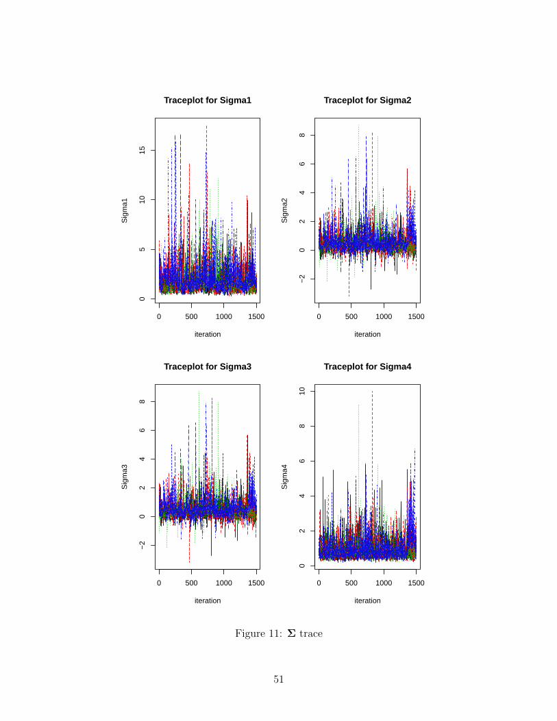
0 500 1000 1500

05

1015

Traceplot for Sigma1

iteration

Sig

ma1

0 500 1000 1500

−2

02

46

8

Traceplot for Sigma2

iteration

Sig

ma2

0 500 1000 1500

−2

02

46

8

Traceplot for Sigma3

iteration

Sig

ma3

0 500 1000 1500

02

46

810

Traceplot for Sigma4

iteration

Sig

ma4

Figure 11: Σ trace

51

H Simulation study details

Each of the one thousand simulations in our simulation study generated a binary undirected

network from the LS-SBM model on three hundred nodes and five equal-sized blocks as

follows. The between-block probability matrix B was:

B =

− 0.3 0.3 0.3 0.3

0.3 − 0.3 0.3 0.3

0.3 0.3 − 0.3 0.3

0.3 0.3 0.3 − 0.3

0.3 0.3 0.3 0.3 −

.

Note that this between-block probability matrix cannot be represented in a two-dimensional

Euclidean latent space since it is impossible to place five points equidistant apart. The

within-block two-dimensional latent space intercept β and scale σ were:

β = (0.6, 2.0, 2.1, 4.0, 4.0)

σ = (0.4, 0.8, 1.2, 1.6, 2.0).

I Approximate computation algorithm

I.1 Two-stage approximate algorithm

The approximate estimation occurs in two stages: 1) the stochastic blockmodel, and 2) the

within-block latent spaces.

The goal of the first stage of the approximate algorithm is to quickly partition the nodes

in to assortative clusters as in a stochastic blockmodel. Any graph clustering algorithm can

in principle be used for this step. For small- and medium-sized networks (e.g. under 1,000

nodes), we have found a variant of spectral clustering designed to find assortative clusters

52

to work well (Saade et al., 2014). This is the algorithm we used in the analysis of the single

Karnataka village and the simulation studies presented in the main text. For large networks,

we have found label propagation (Raghavan et al., 2007) to scale well while still returning

meaningful assortative clusters. This is the algorithm we used to estimate our model on all

75 Karnataka village networks combined (a total of 13,009 nodes).

For the second stage of the two-stage approximation, we estimate each within-block latent

space for the blocks identified by spectral clustering using a variational Bayes algorithm. See

appendix I.2 for the details of this algorithm.

I.2 Variational approximation

For the variational Bayes estimation of the latent space in the two-stage approximate pro-

cedure, we adapt the algorithm developed in Salter-Townshend and Murphy (2013). Since

the latent space associated with each block is estimated independently, we describe the algo-

rithm below for a single block and omit the block subscript k on the block-level parameters

β and σ2.

Let τ = σ−2. For a prior distribution we set τ ∼ Gamma(a0, b0) and β ∼ N(m0, t−10 ). We

use a fixed-form variational approximation with variational family of posterior distributions

defined by τ ∼ Gamma(a, b), β ∼ N(m, t−1), Zi ∼ ND(`i, s−1i ID), and τ, β,Z1, . . . ,Zn

independent. Denote the full set of free variational parameters ψ.

The standard variational criterion function, known as the ELBO, is not available in closed

form for this approximation. We use the same first order Taylor series approximation to the

part of the ELBO concerned with the likelihood of Yij as in Salter-Townshend and Murphy

(2013):

∑i,j

Eψ [log p(Yij|Zi,Zj, β)] ≈∑i,j

[Yijηij − log(1 + exp(ηij))]

53

for

ηij = m+ t−1/2− (‖`i − `j‖2 + (s−1i + s−1

j )d)1/2.

The next part of the ELBO concerns the conditional distribution of Zi:

∑i

Eψ

[log

p(Zi|τ)

q(Zi|`i, si)

]∝∑i

Eη[

12

log τ − τ2N‖Zi‖2 − 1

2log si + si

2‖Zi − `i‖2

]∝∑i

[12ψ(a)− 1

2log b− a

2Nb(ds−1

i + ‖`i‖2)− 12

log si)].

Finally, the KL divergence between prior and posterior:

Eη

[log

p(τ |a0, b0)

q(τ |a, b)+ log

p(β|m0, t0)

q(β|m, t)

]= Eη [a0 log b0 − a log b− log Γ(a0) + log Γ(a)

+(a0 − a) log τ − (b0 − b)τ + 12

log t0 − 12

log t

− t02

(β −m0)2 + t2(β −m)2

]∝ −a log b+ log Γ(a) + (a0 − a)(ψ(a)− log b)

− (b0 − b)ab −12

log t− t02

[(m−m0)2 + t−1].

We use a BFGS algorithm to maximize the ELBO with respect to m, t, a, b, ` and s. Denoting

the ELBO L and differentiating with respect to m and t gives:

∂L

∂m=∑i,j

[Yij − logit−1(ηij)

]− t0(m−m0)

∂L

∂t=

1

2t2

(t0 +

∑i,j

logit−1(ηij)

)− 1

2t.

For a and b we have the derivatives

∂L

∂a= ψ′(a)(a0 + N

2− a)− b−1

(b0 + 1

2NΣi(

Dsi

+ ‖`i‖2))

+ 1.

∂L

∂b= −(a0 + N

2)b−1 + (ab0 + 1

2NΣia(ds−1

i + ‖`i‖2))b−2

54

from which we get the closed form solution a = a0 + N2

. Finally for `i and si we have

∂L

∂`ik=∑j

[−(`ik − `jk)(‖`i − `j‖2 +D(s−1

i + s−1j ))−1/2

(Yij − logit−1(ηij)

)]− a

Nb`ik

∂L

∂si=∑j

[12Ds−2

i (‖`i − `j‖2 +D(s−1i + s−1

j ))−1/2(Yij − logit−1(ηij)

)]+

ad

2Nbs2i

− 1

2si.

55