PDF - arXiv.org e-Print archive · ZHAO et al.: BAYESIAN SPARSE TUCKER MODELS FOR DIMENSION REDUCTION AND TENSOR COMPLETION 2 tion performance, whereas this problem is …

ZHAO et al.: BAYESIAN SPARSE TUCKER MODELS FOR DIMENSION REDUCTION AND TENSOR COMPLETION 1

Bayesian Sparse Tucker Models forDimension Reduction and Tensor Completion

Qibin Zhao, Member, IEEE, Liqing Zhang, Member, IEEE, and Andrzej Cichocki Fellow, IEEE

Abstract—Tucker decomposition is the cornerstone of modern machine learning on tensorial data analysis, which have attractedconsiderable attention for multiway feature extraction, compressive sensing, and tensor completion. The most challenging problem isrelated to determination of model complexity (i.e., multilinear rank), especially when noise and missing data are present. In addition,existing methods cannot take into account uncertainty information of latent factors, resulting in low generalization performance. Toaddress these issues, we present a class of probabilistic generative Tucker models for tensor decomposition and completion withstructural sparsity over multilinear latent space. To exploit structural sparse modeling, we introduce two group sparsity inducing priorsby hierarchial representation of Laplace and Student-t distributions, which facilitates fully posterior inference. For model learning, wederived variational Bayesian inferences over all model (hyper)parameters, and developed efficient and scalable algorithms based onmultilinear operations. Our methods can automatically adapt model complexity and infer an optimal multilinear rank by the principle ofmaximum lower bound of model evidence. Experimental results and comparisons on synthetic, chemometrics and neuroimaging datademonstrate remarkable performance of our models for recovering ground-truth of multilinear rank and missing entries.

Index Terms—Tensor decomposition, tensor completion, Tucker decomposition, multilinear rank, structural sparsity, MRI completion

F

1 INTRODUCTION

T ENSOR decomposition aims to seek a multilinear la-tent representation of multiway arrays, which is a

fundamental technique for modern machine learning ontensorial data mining. In contrast to matrix factorization,tensor decomposition can effectively capture higher orderstructural properties by modeling multilinear interactionsamong a group of low-dimensional latent factors, leadingto significant advantages for multiway dimension reduc-tion [1], multiway regression/classification [2], [3], and com-pressive sensing [4] or completion of structured data [5].In particular, Tucker [6] and Candecomp/Parafac (CP) [7]decompositions have attracted considerable interest in var-ious fields, such as chemometrics, computer vision, socialnetwork analysis, and brain imaging [8], [9], [10].

Tucker decomposition represents an N th-order tensorby multilinear operations between N factor matrices anda core tensor. If we view factor matrices as basis of N latentspace, then core tensor represents a multilinear coefficientfor the whole tensor. An alternative perspective is thatcore tensor is viewed as basis of a latent manifold space,then factor matrices represent low-dimensional coefficientscorresponding to N different profiles for each data point.Tucker decomposition can exactly represent an arbitraryrandom tensor. In contrast, CP decomposition enforces astrict structure assumption by a super-diagonal core tensor,

• Q. Zhao is with Laboratory for Advanced Brain Signal Processing, RIKENBrain Science Institute, Japan and Department of Computer Science andEngineering, Shanghai Jiao Tong University, China.

• L. Zhang is with MOE-Microsoft Laboratory for Intelligent Computingand Intelligent Systems and Department of Computer Science and Engi-neering, Shanghai Jiao Tong University, China.

• A. Cichocki is with Laboratory for Advanced Brain Signal Processing,RIKEN Brain Science Institute, Japan and Systems Research Institute inPolish Academy of Science, Warsaw, Poland.

which is suitable for highly structured data but with limitedgeneralization ability for various types of data. Tensor de-composition becomes interest only when underlying infor-mation has an intrinsic low-rank property, leading to a com-pact representation in latent space. Hence, one fundamentalproblem is separating the information and noise space bymodel selection, i.e., determination of tensor rank, which ischallenging when noise variance is comparable to that ofinformation. Note that tensor rank differs from matrix rankin many mathematic properties [11], [12], [13]. Numerousstudies proposed tensor decomposition methods by eitheroptimization techniques or probabilistic model learning [8],[9], [14], [15], [16], [17]. However, tensor rank is always re-quired to be specified manually. In addition, general modelselection methods need to perform tensor decomposition foreach predefined model, which is inapplicable for Tuckermodel due to that the number of possibilities increasesexponentially with the order of tensors. Some preliminarystudies on automatic model determination were exploitedin [18], [19] which however, may prone to overffing and failto recover true tensor rank in the case of highly noisy data,due to point estimation of model parameters.

Tensor completion can be formulated as tensor decom-position with missing values, which seems fairly straightfor-ward but has several essential differences. Tensor decompo-sition focusing on data representation is referred to unsu-pervised technique, whereas tensor completion focusing onpredictive ability is referred to semi-supervised technique,which aims to predict tensor elements from their N -tupleindices. Another important issue is that the optimal tensorrank for tensor completion is related to missing ratio andmay differ from the underlying true rank that is alwaysoptimum for tensor decomposition. Hence, the key problemof tensor completion is to choose an appropriate tensor rank(i.e., model complexity) that can obtain optimal generaliza-

arX

iv:1

505.

0234

3v1

[cs

.LG

] 1

0 M

ay 2

015


tion performance, whereas this problem is more challengingas compared to tensor decomposition for a fully observedtensor. More specifically, existing model selections includingcross-validation are not applicable due to correlations be-tween the optimal tensor rank and number of observed datapoints. Although numerous tensor decomposition methodsfor partially observed tensor were developed in [20], [21],[22], [23], [24], [25], [26], the most challenging task of speci-fying tensor rank was conveyed to user, and thus was donemostly based on an implicit assumption that missing datais known. Several studies have considered automatic rankdetermination for CP decomposition [5], [27]. In contrastto CP rank, multilinear rank has more degree of freedom.An alternative framework for tensor completion, based ona low-rank assumption, was developed by minimizing thenuclear norm of approximate tensor, which corresponds toa convex relaxation of rank minimization problem [28]. Al-though this technique successfully avoids specifying tensorrank manually, several tuning parameters are required andsensitive to missing ratio. Hence, it essentially transformedthe model selection problem to a parameter selection prob-lem. The nuclear norm based tensor completion was shownto be attractive in recent years [29], [30], [31], [32], [33], [34].Many variants by imposing additional constraints were alsoexploited in [35], [36] which have shown advantages forsome specific type of data. However, the best performancewas mostly obtained by carefully tuning parameters basedon implicit assumption that missing data is known. Anotherissue is that the definition of nuclear norm of tensor cor-responds to a (weighted) summation of mode-n rank Rndenoting the dimension of latent factor matrices. However,the dimension of core tensor

∏nRn represents the model

complexity of whole tensor as described previously. As aresult, another possible framework can be introduced byoptimization of logarithm transformed nuclear norm.

In this paper, we present a class of generative models forTucker representation of a complete or incomplete tensorcorrupted by noise, which can automatically adapt modelcomplexity and infer an optimal multilinear rank solelyfrom observed data. To achieve automatic model determi-nation, we investigate structural sparse modeling throughformulating Laplace as well as Student-t distributions in ahierarchial representation to facilitate full posterior infer-ence, which therefore can be further extended to enforcegroup sparsity over factor matrices and structural sparsityover core tensor. For model learning, we derive the fullposterior inference under a variational Bayesian framework,including remarkable inference for the non-conjugate hi-erarchical Laplace prior. Finally, all model parameters canbe inferred as well as predictive distribution over missingdata without needing of tuning parameters. In addition, weintroduce several Theorems based on multilinear operationsto improve computational efficiency and scalability.

The rest of this paper is organized as follows: Section 2presents notations and multilinear operations. In Section 3,we present group sparse modeling by hierarchical sparsityinducing priors. Section 4 presents Bayesian Tucker modelfor tensor decomposition, while Section 5 presents BayesianTucker model for tensor completion. The algorithm relatedissues are discussed in Section 6. Section 7 shows experi-mental results followed by conclusion in Section 8.

2 PRELIMINARIES AND NOTATIONS

Let X ,X,x denote a tensor, matrix, vector respectively.Given an N th-order tensor X ∈ RI1×I2×···×IN , its(i1, . . . , iN )th entry is denoted by Xi1···iN , where in =1, . . . , In, n = 1, . . . , N . The standard Tucker decompositionis defined by

X = G ×1 U(1) ×2 U(2) × · · · ×N U(N). (1)U(n) ∈ RIn×Rn

Nn=1

are a set of mode-n factor ma-trices, G ∈ RR1×R2×···×RN denotes the core tensor and(R1, . . . , RN ) denote the dimensions of mode-n latentspace, respectively. The overall model complexity can berepresented by

∏nRn or

∑nRn, whose minimum as-

sociated values RnNn=1 is termed as multilinear rank oftensor X [9]. For a specific U(n), we denote its row vec-tors by

u

(n)in

∣∣in = 1, . . . , In

and its column vectors byu

(n)·rn∣∣rn = 1, . . . , Rn

.

Definition 2.1. LetU(n) ∈ RIn×Rn

Nn=1

denote a set ofmatrices, the sequential Kronecker products in a reversedorder is defined and denoted by⊗

n

U(n) = U(N) ⊗U(N−1) ⊗ · · · ⊗U(1).⊗k 6=n

U(k) = U(N) ⊗ · · · ⊗U(n+1) ⊗U(n−1) ⊗ · · · ⊗U(1).

The symbol ⊗ denotes Kronecker product.⊗

n U(n) is amatrix of size (

∏n In ×

∏nRn).

The Tucker decomposition (1) can be also represented byusing matrix, vector, or element-wise forms, given by

X(n) = U(n)G(n)

(⊗k 6=n

U(k)T

),

vec(X ) =

(⊗n

U(n)

)vec(G),

Xi1···iN =

(⊗n

u(n)Tin

)vec(G).

(2)

It should be noted that the multilinear operation is signifi-cantly efficient for computation. For example, if we compute⊗

n U(n) firstly and then multiply it with vec(G), both thecomputation and memory complexity is O (

∏n InRn). In

contrast, if we apply a sequence of multilinear operations(·) ×n U(n) without explicitly computing

⊗n U(n), the

computational complexity is O (minn(Rn)∏n In) while the

memory cost is O(∏n In). In this paper, we use notation⊗

n(·) frequently for clarity, however, the implementationcan be performed by using multilinear operations.

3 HIERARCHICAL GROUP SPARSITY PRIORS

The sparsity inducing priors are considerably importantand powerful for many machine learning models. The mostpopular ones are Laplace, Student-t, and Spike and slabpriors. However, these priors are often not conjugate withthe likelihood distribution, which leads to difficulties forfully Bayesian inference. In contrast, another popular spar-sity inducting prior is automatic relevance determination(ARD), which has been widely applied in many powerful


methods such as relevance vector machine and Bayesianprinciple component analysis [37], [38], [39]. The advantagesof ARD prior lie in its conjugacy resulted from a hierarchicalstructure. Note that ARD prior is essentially a hierarchicalStudent-t distribution since its marginal distribution is∫ ∞

0N (x|0, λ−1)Ga(λ|a, b) dλ = T (x|0, ab−1, 2a). (3)

Ga(x|a, b) = ba

Γ(a)xa−1e−bx denotes a Gamma distribution

and T (x) denotes a Student-t distribution. One can showthat when a noninformative prior is specified by a = b→ 0,then p(x) ∝ 1/|x|, which indicates the sparsity inducingproperty of a hierarchial Student-t prior.

A straightforward question is that can we representLaplace prior by the hierarchical distributions which areconjugate? As shown in [40], [41], a hierarchical structureof Gaussian and Exponential distributions yields a Laplacemarginal distribution, whereas they are not conjugate pri-ors. In this paper, we present another hierarchial Laplacedistribution by employing an Inverse Gamma distributionIG(x|a, b) = ba

Γ(a)x−a−1e−bx

−1

. By a specific setting of

IG(1, γ2 ) = γ2x−2e−

γ2 x

−1

, we can show that the marginaldistribution is∫ ∞

0N (x|0, λ−1)IG(λ|1, γ

2) dλ = Laplace

(x|0, 1√γ

). (4)

Note that γ govern the degree of sparsity, for example,if γ = 1, then p(x) ∝ e−|x|. To avoid parameter selec-tion manually, we can place a noninformative prior overγ and employ Bayesian inference for posterior estimation.Although inverse Gamma is a non-conjugate prior, we caninfer its variational posterior represented by a more gener-alized distribution.

Let x = x1, . . . , xR denote a set of random variables,the hierarchical sparsity inducing priors can be specified as∀r = 1, . . . , R,

Student-t: xr ∼ N (0, λ−1r ), λr ∼ Ga(a, b), (5)

Laplace: xr ∼ N (0, λ−1r ), λr ∼ IG(1,

γ

2). (6)

Hence, the marginal distributions of x can be found by(3), (4) as p(x) =

∏Rr=1 T (xr|0, ab−1, 2a) and p(x) =∏R

r=1 Laplace(xr|0, 1√γ ).

Now we consider to extend the above hierarchical priorsfor group sparse modeling. Let X = x1, . . . ,xR denoteR groups of random variables where xr ∈ RIr denote rthgroup that contains Ir random variables. Note that I1 =I2 · · · = IR is not necessary. The group sparse modeling isto enforce sparsity on groups in contrast to the individualrandom variables, which effectively take into account theclustering properties of relevant variables. To employ thehierarchial sparsity priors for group sparse model, it can bespecified as ∀r = 1, . . . , R,

Student-t: xr ∼ N (0, λ−1r IIr ), λr ∼ Ga(a, b), (7)

Laplace: xr ∼ N (0, λ−1r IIr ), λr ∼ IG(1,

γ

2). (8)

Therefore, the marginal distributions of X can be de-rived as p(X ) =

∏Rr=1 T (xr|0, ab−1, 2a) and p(X ) =

∏Rr=1 Laplace(xr|0, 1√

γ ), where T (x), Laplace(x) denotea multivariate Student-t distribution and a multivariateLaplace distribution respectively [42]. One can show thatwhen a = b → 0, then ∀r, p(xr) ∝ (1/‖xr‖2)Ir . Whenγ → 1, then ∀r, p(xr) ∝ e−‖xr‖2 .

In the following sections, we employ both hierarchialStudent-t and hierarchial Laplace priors to impose groupsparsity over multi-mode latent factors, yielding the mini-mum latent dimensions, for tensor decomposition models.

4 BAYESIAN TUCKER MODEL FOR TENSOR DE-COMPOSITION

4.1 Model specification

We first consider the Bayesian Tucker model for an N th-order tensor Y ∈ RI1×···×IN that is fully observed. Weassume that Y is a measurement of the latent tensor Xcorrupted by i.i.d. Gaussian noises, i.e., Y = X+ε, where Xis generated exactly by the Tucker representation as shownin (1). Therefore, the observation model can be specified bya vectorized form,

vec(Y)∣∣∣U(n)

,G, τ ∼ N

((⊗n

U(n))

vec(G), τ−1I

).

(9)Our objective is to infer the model parameters, as well asmodel complexity, automatically and solely from given data.To this end, we propose the hierarchical prior distributionsover all model (hyper)parameters. For noise precision τ , aGamma prior can be simply placed with appropriate hyper-parameters, yielding an noninformative prior distribution.

To modeling tensor data by an appropriate model com-plexity, it is important to design the flexible prior dis-tributions over the group of factor matrices U(n), n =1, . . . , N , and the core tensor G, whose complexity can beadapted to a specific given tensor. Since the model complex-ity of Tucker decompositions depends on the dimensions ofG, denoted by (R1, R2, . . . , RN ), while Rn, n = 1, . . . , Nalso corresponds to the number of columns in model-nfactor matrix U(n) and thus represents the dimensions ofmode-n latent space. The minimal number of RnNn=1 i.e.,multilinear rank [9] usually need to be given in advance.However, due to the presence of noise, the optimal selectionof multlinear rank is quite challenging. Although somemodel selection criterions can be applied, the accuracy sig-nificantly depends on the decomposition algorithms, result-ing in less stability and high computational cost. Therefore,we seek an elegant automatic model selection, which cannot only infer the multilinear rank, but also effectively avoidoverfitting. To achieve this, we employ the proposed groupsparsity priors over factor matrices. More specifically, eachU(n) is govern by hyperparameters λ(n) ∈ RRn , where λ(n)

rn

controls the precision related to rn group (i.e., rnth column).Due to the group sparsity inducing property, the dimensionsof latent space will be enforced to be minimal. On the otherhand, the core tensor G also needs to be as sparse as possi-ble. However, if we straightforwardly place an independentsparsity prior, the interactions between G and U(n) can-not be modeled, which may lead to inaccurate estimationof multilinear rank. As Gr1,...,rN can be considered as the


scalar coefficient of the rank-one tensor u(1)·r1 ⊗ · · · ⊗ u

(N)·rN

that involves rnth group from each of U(n), respectively.Taken into account the fact that if ∃n, ∃rn,u(n)

·rn = 0, thenGr1,...,rN should be also enforced to be zero, the precisionparameter for Gr1,...,rN can be specified as the product ofprecisions over u(n)

·rnNn=1, which is represented by

Gr1···rN∣∣∣ λ(n)

, β ∼ N

(0,(β∏n

λ(n)rn

)−1), (10)

where β is a scale parameter related to the magnitude ofG, on which a hyperprior can be placed. The hyperprior forλ(n) play a key role for different sparsity inducing priors.We propose two hierarchial priors including Student-t andLaplace for group sparsity. Let Λ(n) = diag(λ(n)), we canfinally specify the hierarchial model priors as

τ ∼ Ga(aτ0 , b

τ0

),

vec(G)∣∣∣ λ(n)

, β ∼ N

0,

(β⊗n

Λ(n)

)−1 ,

β ∼ Ga(aβ0 , b

β0

),

u(n)in

∣∣λ(n) ∼ N(0, Λ(n)−1

), ∀n, ∀in,

Student-t: λ(n)rn ∼ Ga

(aλ0 , b

λ0

), ∀n, ∀rn,

Laplace: λ(n)rn ∼ IG

(1,γ

2

), ∀n, ∀rn,

γ ∼ Ga(aγ0 , bγ0).

(11)

The prior for the core tensor G is written as a tensor-variate Gaussian distribution. The observation model in (9)and the hierarchial priors in (11) are integrated, which istermed as Bayesian Tucker Decomposition (BTD) model.Note that there are two proposed hierarchial sparsity priorsin BTD model, which are thus denoted respectively by BTD-T (Student-t priors) and BTD-L (Laplace priors).

For simplicity, all unknown (hyper)parameters inBTD model are collected and denoted by Θ =G,U(1), . . . ,U(N),λ(1), . . . ,λ(N), τ, β, γ. Thus the jointdistribution of BTD model is written as

p(Y ,Θ) = p(Y |U(n),G, τ

)∏n

p(U(n)

∣∣λ(n))× p(G∣∣Λ(n), β

)∏n

p(λ(n)|γ

)p(γ)p(β)p(τ). (12)

In general, maximum a posterior (MAP) of Θ can be esti-mated by optimizations of logarithm joint distribution w.r.t.each parameters alternately. However, due to the propertyof point estimation, MAP is still prone to overfitting. In con-trast, we aim to infer the posterior distributions of Θ undera fully Bayesian treatment, which is p(Θ|Y) = p(Θ,Y)∫

p(Θ,Y) dΘ.

4.2 Model inference

The model learning can be performed by the approximateBayesian inferences when the posterior distributions areanalytically intractable. Since the variational Bayesian in-ference [43] is more efficient and scalable as compared tosampling based inference methods, we employ VB tech-nique to learn both BTD-T and BTD-L models. It should benoted that the hierarchial Laplace priors are not conjugate,

resulting in a challenging problem to be addressed. In thissection, we present the main solutions for model inferencewhile the detailed derivations and proofs are provided inthe Appendix.

VB inference aims to seek an optimal q(Θ) to ap-proximate the true posterior distribution in the senseof minKL(q(Θ)||p(Θ|Y)). Since KL(q(Θ)||p(Θ|Y)) =ln p(Y) − L(q), the optimum of q(Θ) can be achieved bymaximization of lower bound L(q) that can be computedexplicitly. To achieve this, we assume that the variationalapproximation posteriors can be factorized as

q(Θ) = q(G)q(β)∏n

q(U(n)

)∏n

q(λ(n))q(γ)q(τ). (13)

Then, the optimized form of jth parameters based onmaxq(Θj) L(q) is given by

qj(Θj) ∝ expEq(Θ\Θj) [ln p(Y ,Θ)]

. (14)

Eq(Θ\Θj)[·] denotes an expectation w.r.t. q distribution overall variables in Θ except Θj . In the following, we use E[·] todenote the expectation w.r.t. q(Θ) for simplicity.

As can be derived, the variational posterior distributionover the core tensor G is

q(G) = N(

vec(G)∣∣vec(G),ΣG

), (15)

where the posterior parameters can be updated by

vec(G) = E[τ ] ΣG

(⊗n

E[U(n)T

])vec (Y) , (16)

ΣG =

E[β]

⊗n

E[Λ(n)

]+ E[τ ]

⊗n

E[U(n)TU(n)

]−1

. (17)

Most of expectation terms in (16), (17) are the functionslinearly related to the corresponding Θj , which can thus beeasily evaluated from their posterior q(Θj). For example,E[U(n)T ] can be evaluated according to q(U(n)) shownin (18), as can be similarly computed for E[τ ], E[β], andE[Λ(n)]. It should be noted that the expectation involv-ing a quadratic term can be evaluated explicitly by usingE[U(n)TU(n)] = E[U(n)T ]E[U(n)] + InΨ(n), which requiresthe posterior parameters given in (18).

The computational complexity for posterior update ofG is O

(∏nR

3n +

∏n InRn

)that polynomially scales with

model complexity denoted by∏nRn and linearly scales

with data size denoted by∏n In. In general, it is dominated

by O(∏

nR3n

), which is related to the matrix inverse. The

memory cost is O(∏

nR2n +

∏n InRn

), dominated by ΣG

and ⊗n(·). It should be noted that multilinear operationsY×1E[U(1)T ]×· · ·×N E[U(N)T ] can be performed withoutexplicitly computing ⊗nE[U(n)T ], thus reducing the mem-ory cost to O

(∏nR

2n +

∏n In

)and also reducing computa-

tion complexity to O(∏nR

3n +

∏n In). To further improve

computation and memory efficiency, we introduce severalimportant Theorems as follows.


Theorem 4.1. LetΣ(n) be a set of diagonalizable matrices,

and c1, c2 denote arbitrary scalars. If ∀n = 1, . . . , N , the spectraldecompositions are represented by Σ(n) = V(n)D(n)V(n)T , then(

c1I + c2⊗n

Σ(n)

)−1

=(⊗n

V(n)

)(c1I + c2

⊗n

D(n)

)−1(⊗n

V(n)T

).

Proof. See Appendix for the detailed proof.

Theorem 4.2. LetΛ(n) be a set of diagonal matrices,

Σ(n)

be a set of diagonalizable matrices, and c1, c2 be scalars. If∀n = 1, . . . , N , the spectral decompositions are represented by

Λ(n)−12Σ(n)Λ(n)−

12

= V(n)D(n)V(n)T , then(c1⊗n

Λ(n) + c2⊗n

Σ(n)

)−1

=(⊗n

Λ(n)− 1

2V(n)

)(c1I + c2

⊗n

D(n)

)−1(⊗n

V(n)TΛ(n)− 1

2

).

Proof. See Appendix for the detailed proof.

Based on Theorem 4.1 and 4.2, ΣG can be factorized asthe product of sequential Kronecker products, which leadsto that matrix inverse operations can be performed by indi-vidual eigenvalue decompositions on N small matrices, andinverse operations only on a diagonal matrix. Therefore, thecomputational complexity for inference of G can be signif-icantly reduced to O

(∑nR

3n +

∏n In

)while the memory

cost can be significantly reduced to O(∑nR

2n +

∏n In), if

we save ΣG by a format of sequential Kronecker products.As can be derived, the variational posterior distribution

over the factor matricesU(n)

is represented by

q(U(n)

)=

In∏in=1

N(u

(n)in

∣∣∣u(n)in,Ψ(n)

), n = 1, . . . , N, (18)


U(n) = E[τ ] Y(n)

⊗k 6=n

E[U(k)

] E[GT

(n)

]Ψ(n), (19)

Ψ(n) =

E[Λ(n)]+ E[τ ]E

G(n)

⊗k 6=n

U(k)TU(k)

GT(n)

−1

.

(20)

In (20), the most complex expectation term related tomultilinear operations can be computed by

vec

E

G(n)

⊗k 6=n

U(k)TU(k)

GT(n)

= E

[G(n) ⊗G(n)

]vec

⊗k 6=n

E[U(k)TU(k)

] . (21)

Thus, each posterior expectation term can be evaluatedeasily according to the corresponding posterior distributionsq(G) and q(U(k)), k = 1, . . . , N, k 6= n.

Taken into account the computation and memory ef-ficiency, multilinear operations and sequential Kroneckerproducts format must be employed to avoid explicitlycomputation of sequential Kronecker products. It shouldbe noted that (21) cannot be factorized into operationson individual kronecker terms because of E

[G(n) ⊗G(n)

].

To reduce the memory cost, we may approximate it byE[G(n)

]⊗E

[G(n)

]. Therefore, the computational complex-

ity for inference of U(n) can be improved to O(R3n+

∏n In)

while the memory cost is O (∏nRn +

∏n In).

The variational posterior distribution over β can bederived to be a Gamma distribution due to its conjugateprior, which is denoted by q(β) = Ga(aβM , b

βM ) where the

posterior parameters can be updated by

aβM = aβ0 +1

2

∏n

Rn,

bβM = bβ0 +1

2E[vec(G2)T

]⊗n

E[λ(n)

].

(22)

In (22), E[vec(G2)T

]= vec(E[G]2)T +diag(ΣG)T should be

applied for rigorous inference, whereas an alternative ap-proximation is E

[vec(G2)T

]= vec(E[G]2)T for efficiency.

E[λ(n)] can be easily evaluated according to q(λ(n))described in the following paragraphs. The computationalcomplexity in (22) is O(

∏nRn).

The inference of hyperparameters λ(n) plays a keyrole for automatic model selection (i.e., determination ofmultilinear rank). In BTD models, as we proposed two hier-archical sparsity priors, resulting in two different posteriordistributions for λ(n).

BTD-T model using hierarchial Student-t priors. As can bederived, the variation posterior distribution over λ(n)is i.i.d. Gamma distributions due to the conjugate priors,which is ∀n = 1, . . . , N ,

q(λ(n)) =

Rn∏rn=1

Ga(λ(n)rn

∣∣a(n)rn , b

(n)rn

), (23)


a(n)rn = aλ0 +

1

2

In +∏k 6=n

Rk

,b(n)rn = bλ0 +

1

2E[u(n)T·rn u(n)

·rn

]+

1

2E[β]E

[vec(G2

···rn···)T]⊗k 6=n

E[λ(k)

].

(24)

According to q(U(n)) described in (18), we obtain that

E[u(n)T·rn u(n)

·rn]

= In(Ψ(n)

)rnrn

+ u(n)T·rn u(n)

·rn . (25)

This represents the posterior expectation of squared L2-norm of rth component in mode-n factors, which also takesinto account the uncertainty information. E

[vec(G2

···rn···)T]

represents the posterior expectation of squared L2-normof rn slice of core tensor G. Therefore, an intuitive inter-pretation of automatic model selection is that the smallerof∥∥u(n)·r∥∥2

Fand ‖G···rn···‖2F leads to larger E[λ

(n)rn ] and

updated prior for p(u

(n)·rn∣∣λ(n)rn ) as well as p(G···rn···|λ

(n)rn ),


which in turn enforces more strongly u(n)·rn and G···rn··· to

be zero. After several iterations, the unnecessary columns infactor matrices and unnecessary slices in core tensor can bereduced to exact zero (i.e., smaller than machine precision).The computational complexity for inference of q(λ(n)) isO(∏nRn + InRn). Given updated parameters for q(λ(n)),

we can evaluate the posterior expectations by E[λ(n)] =[a

(n)1 /b

(n)1 , . . . , a

(n)Rn/b

(n)Rn

]Tand E[Λ(n)] = diag(E[λ(n)]).

BTD-L model using hierarchial Laplace priors. Since thehierarchical Laplace prior is not conjugate, which leads tomuch difficulties for model inference. To solve this prob-lem, we employ a generalized inverse Gaussian distribu-tion, denoted by GIG(x|h, a, b), which includes Gamma,inverse Gamma, and inverse Gaussian distribution as spe-cial cases by an appropriate setting of hyperparameters.For example, one can show that Ga(a, b) = GIG(a, 2b, 0)and IG(a, b) = GIG(−a, 0, 2b). For BTD-L mode, we keepusing λ

(n)rn ∼ IG(1, γ2 ) as the hyper-prior, however the

variational posterior q(λ(n)rn ) cannot be represented as an

inverse Gamma distribution.As can be derived, the variation posterior distribution

over λ(n) can be represented as i.i.d. GIG distributions,which is ∀n = 1, . . . , N ,

q(λ(n)) =

Rn∏rn=1

GIG(λ(n)rn

∣∣h, a(n)rn , b

(n)rn

), (26)


h =1

2

In +∏k 6=n

Rk

− 1, b(n)rn = E[γ],

a(n)rn = E[β]E

[vec(G2

···rn···)T]⊗k 6=n

E[λ(k)

]+ E

[u(n)T·rn u(n)

·rn

].

(27)

The computational complexity for inference of q(λ(n)) isalso O(

∏nRn + InRn). Given the updated parameters,

we can evaluate EGIG[λ

(n)rn

]straightforwardly, while an

alternative approximation is the posterior mode w.r.t. GIGdistribution that can avoid computational instabilities ofmodified Bessel function.

By comparing (26) with (23), we can investigate the es-sential difference between Student-t and Laplace priors. Onecan show that (23) can be rewritten as GIG

(a

(n)rn , 2b

(n)rn , 0

)with parameters given by (24). Hence, the key difference liesin the setting of γ. If γ = 0, Student-t and Laplace priors areessentially equivalent. To avoid manually tuning parame-ters, we also place a hyper-prior over γ and thus derivethe variational posterior distribution as q(γ) = Ga(aγM , b

γM )

whose posterior parameters can be updated by

aγM = aγ0 +N∑n=1

Rn,

bγM = bγ0 +1

2

N∑n=1

Rn∑rn=1

E[λ(n)−1

rn

].

(28)

It should be noted that E[λ

(n)−1

rn

]cannot be computed

straightforwardly by E[λ

(n)rn

]−1. Since q(λ

(n)rn ) is a GIG

distribution as shown in (26), it is not difficult to derivethat q

(λ

(n)−1

rn

)= GIG(−h, b(n)

rn , a(n)rn ), yielding the posterior

expectation computed by

EGIG[λ(n)−1

rn

]=

√a

(n)rn K1−h

(√a

(n)rn b

(n)rn

)√b(n)rn K−h

(√a

(n)rn b

(n)rn

) , (29)

and the posterior mode computed by

arg maxλ(n)−1rn

GIG(λ(n)−1

rn

)=

(−h− 1) +

√(−h− 1)2 + a

(n)rn b

(n)rn

b(n)rn

,

(30)

where K1−h(·) denotes a modified Bessel function of thesecond kind.

As can be derived, the variational posterior distribu-tion over the noise hyperparameter is q(τ) = Ga(aτM , b

τM )

whose parameters can be updated by

aτM = aτ0 +1

2

∏n

In,

bτM = bτ0 +1

2E

[∥∥∥∥∥vec(Y)−

(⊗n

U(n)

)vec(G)

∥∥∥∥∥2

F

],

(31)

where the posterior expectation of model residuals can beevaluated by

E

[∥∥∥∥∥vec(Y)−

(⊗n

U(n)

)vec(G)

∥∥∥∥∥2

F

]=

‖Y‖2F − 2vec(Y)T(⊗

n

E[U(n)]

)E[vec(G)]

+ Tr

(E[vec(G)vec(G)T

]⊗n

E[U(n)TU(n)

]). (32)

In principle, E[vec(G)vec(G)T

]= vec(G)vec(G)T + ΣG.

However, vec(G)vec(G)T can be alternatively used as anapproximation, which then makes it possible to applymultilinear operations for computing (32) quite efficiently.Hence, the computational complexity can then be reducedto O(

∏nRn +

∏n In).

The inference framework presented in this section canessentially maximize the lower bound of model evidencewhich is defined by L(q) = Eq(Θ)[ln p(Y ,Θ)] + H(q(Θ)).The first term denotes the posterior expectation of jointdistribution while the second term denotes the entropy ofq(Θ). In principle, L(q) should increase at each iteration,thus it can be used to test for convergence. We provide thedetailed computation forms of L(q) in the Appendix.

5 BAYESIAN TUCKER MODEL FOR TENSOR COM-PLETION

5.1 Model specificationIn this section, we consider Bayesian Tucker model fortensor completion. Let Y denotes an incomplete tensor(i.e., with missing entries), and O denotes a binary tensorindicating the observation positions, i.e., Oi1···iN = 1 if(i1, . . . , iN ) ∈ Ω otherwise it is zero. Ω denotes a set of N -tuple indices of observed entries. YΩ denotes only observed


entries. Similar to BTD model, we assume a generativemodel YΩ = XΩ + ε where the latent tensor X can be rep-resented exactly by a Tucker model with a low multilinearrank and ε denotes i.i.d. Gaussian noise.

Given an incomplete tensor, Bayesian Tucker model onlyconsiders the observed entries, yielding a new likelihoodfunction represented by

p(YΩ|U(n),G, τ

)=

∏(i1,...,iN )∈Ω

N(Yi1...iN |Xi1...iN , τ−1

).

Based on Tucker decomposition framework, we can thusrepresent the observation model as that ∀(i1, . . . , iN ),

Yi1···iN∣∣∣ u

(n)in

,G, τ ∼ N

((⊗n

u(n)Tin

)vec(G), τ−1

)Oi1···iN

.

(33)

For Tucker decomposition of an incomplete tensor, theproblem is ill-conditioned and has infinite solutions. Thelow-rank assumption play an key role for successful tensorcompletion, which implies that the determination of multi-linear rank significantly affects the predictive performance.However, standard model selection strategies, such as cross-validation, cannot be applied for finding the optimal mul-tilinear rank because it varies dramatically with missingratios. Therefore, the inference of multilinear rank is morechallenging when missing values occur.

As described in BTD model, we employ two types ofhierarchical group sparsity priors over the factor matricesand core tensor with aim to seek the minimum multilinearrank automatically, which is more efficient and elegant thanthe standard model selections by repeating many times andselecting one optimum model. Therefore, the model priorsfor all hidden variables are same with that in BTD model. Bycombining likelihood model in (33) with the model priorsin (11), we propose a Bayesian Tucker Completion (BTC)model, which enable us to infer the minimum multilinearrank as well as the noise level solely from partially observeddata without requiring any tuning parameters.

5.2 Model inferenceFor BTC model, we also employ VB inference frameworkto learn the model under a fully Bayesian treatment. SinceBTC model differs from BTD model in the likelihood func-tion (33), indicating that the inference for factor matrices,core tensor and noise parameter are essentially different,while other hyperparameters can be inferred by the samesolutions. In this section, we present only the main solu-tions while the detailed derivations are provided in theAppendix.

As can be derived, the variational posterior distributionover the core tensor G is

q(G) = N(

vec(G)∣∣vec(G),ΣG

)(34)


vec(G) = E[τ ] ΣG∑

(i1,...,iN )∈Ω

(Yi1···iN

⊗n

E[u

(n)in

])(35)

ΣG =

E[β]⊗n

E[Λ(n)

]+ E[τ ]

∑(i1,...,iN )∈Ω

⊗n

E[u

(n)in

u(n)Tin

]−1

(36)

It should be noted that Theorems 4.1, 4.2 and multilinearoperations cannot be applied to (36) due to the sum ofkronecker products. Thus the sequential kronecker productsmust be computed explicitly, resulting in the computationalcost of O

(∏nR

3n +M

∏nR

2n

), where M denotes the num-

ber of observed entries (i.e., data size), and memory costof O

(∏nR

2n

). This severely prevents the method from

being applied to large-scale datasets. To improve scala-bility, we propose an alternative solution by optimizingargminG− ln q(G) instead of closed-form update in (35).This can be achieved by employing a nonlinear conjugategradient method with the gradient given by

∂ − ln q(G)∂(vec(G))

= E[β]

(⊗n

E[Λ(n)

])vec(G)

+ E[τ ]∑

(i1,...,iN )∈Ω

(⊗n

E[u

(n)in

u(n)Tin

])vec(G)

− E[τ ]∑

(i1,...,iN )∈Ω

(Yi1···iN

⊗n

E[u

(n)in

])(37)

Thus, multilinear operations can be applied without explic-itly computation of kronecker products, resulting in reducedcomputational complexity of O (M

∏nRn) and reduced

memory cost of O (∏nRn), which scales linearly with data

size and model complexity.As can be derived, the variational posterior distribution

overU(n)

is factorized as

q(U(n)

)=∏in

N(u

(n)in

∣∣∣u(n)in,Ψ

(n)in

), n = 1, . . . , N, (38)


u(n)in

= E[τ ]Ψ(n)in

E[G(n)

] ∑(i1,...,iN )∈Ω

Yi1···iN ⊗k 6=n

E[u

(k)ik

](39)

Ψ(n)in

=E[Λ(n)] + E[τ ]E

[G(n)Φ

(n)in

GT(n)

]−1

(40)

where Φ(n)in

=∑

(i1,...,iN )∈Ω

⊗k 6=n

u(k)ik

u(k)Tik

, the summation is

performed over the observed data locations whose mode-nindex is fixed to in. In other words, Φ

(n)in

represents thestatistical information of mode-k (k 6= n) latent factors thatinteract with u

(n)in

. In (40), the complex posterior expectationcan be computed by

vecE[G(n)Φ

(n)in

GT(n)

]= E

[G(n) ⊗G(n)

]vec

(Φ

(n)in

). (41)

The computational complexity for inference of u(n)in

isO(R3n +M

∏nRn

), while the memory cost is O(

∏nRn).

An intuitive interpretation of (40) is that the posteriorcovariance Ψ

(n)in

combines prior information denoted byE[λ(n)] and posterior information of interacted factors inother modes, while the tradeoff between these two terms iscontrolled by model residual E[τ ]. Hence, if updated E[λ(n)

rn ]is quite large and model is not well fitted, then the posteriorvariance of rnth component will be easily forced to zero.


Given updated q(u

(n)in

)from (38), we can easily compute

the posterior expectations of some expressions as

E[u(n)T·rn u(n)

·rn]

= u(n)T·rn u(n)

·rn +∑in

(Ψ

(n)in

)rnrn

,

E[u

(n)in

u(n)Tin

]= u

(n)in

u(n)Tin

+ Ψ(n)in.

(42)

The variational posterior distribution over noise preci-sion τ can be derived as q(τ) = Ga(τ |aτM , bτM ) whoseparameters are updated by

aτM = aτ0 +1

2

∑i1,...,iN

Oi1···iN ,

bτM = bτ0 +1

2E

∑(i1,...,iN )∈Ω

(Yi1···iN −

(⊗n

u(n)Tin

)vec(G)

)2

(43)

The posterior expectation of model residuals over observedentries can be evaluated by

E

∑(i1,...,iN )∈Ω

(Yi1···iN −

(⊗n

u(n)Tin

)vec(G)

)2 =

‖YΩ‖2F − 2

∑(i1,...,iN )∈Ω

Yi1···iN⊗n

E[u

(n)Tin

]E[vec(G)]

+ Tr

E[vec(G)vec(G)T

] ∑(i1,...,iN )∈Ω

⊗n

E[u

(n)in

u(n)Tin

] .

(44)

The computational complexity is O(M∏nRn), if multilin-

ear operations have been applied.Note that other hidden hyperparameters in Θ except

G, U(n), τ can be inferred essentially by the same so-lutions with BTD model. In addition, the lower boundL(q) = Eq(Θ)[ln p(YΩ,Θ)] +H(q(Θ)) can be also evaluatedwith different expressions related to G, U(n), τ (seeAppendix for details).

The predictive distributions over missing entries, givenobserved entries, can be approximated by using variationalposterior distributions q(Θ) as follows

p(Yi1···iN |YΩ) =

∫p(Yi1···iN |Θ)p(Θ|YΩ) dΘ

≈ N(Yi1···iN

∣∣∣Yi1···iN , E[τ ]−1 + σ2i1···iN

),

(45)

where the posterior parameters can be obtained by

Yi1···iN =

(⊗n

E[u

(n)Tin

])E[vec(G)]

σ2i1···iN = Tr

(E[vec(G)vec(G)T

]⊗n

E[u

(n)in

u(n)Tin

])

−E[vec(G)]T(⊗

n

E[u

(n)in

]E[u

(n)Tin

])E[vec(G)].

(46)

Therefore, our model can provide not only predictions overmissing entries, but also the uncertainty of predictions,which is quite important for some specific applications.

6 ALGORITHM RELATED ISSUES

We denote Bayesian sparse Tucker models (i.e., BTD andBTC) when two different group sparsity priors have beenemployed by BTD-T, BTD-L, BTC-T, BTC-L respectively,where T, L represent a hierarchical Student-t and Laplacepriors. The main procedure of model inference is describedas follows:

• Setting of top-level hyperparameters. For BTD-T and BTC-T models, aτ0 , bτ0 , a

β0 , b

β0 , a

λ0 , b

λ0 are

set to 1e-9. For BTD-L and BTC-L models,aτ0 , bτ0 , a

β0 , b

β0 , a

γ0 , b

γ0 are set to 1e-9. This setting

results in a noninformative prior, which ensures thatmodel inference is solely based on observed data.

• Initialization of hidden parameters Θ. For BTD-Tand BTC-T, Θ = G, U(n), λ(n), τ, β. For BTD-L and BTC-L, Θ = G, U(n), λ(n), τ, β, γ. Gdoes not need to be initialized due to that it willbe updated firstly. The latent dimensions can beinitialized by Rn = In,∀n or manually by Rn < In.U(n) can be initialized as left singular vectors bymode-n SVD, while an alternative one is samplingfrom N (0, 1). τ is initialized by 1/σ2

Y denoting aninverse of data variance. λ(n), β, γ are simply ini-tialized to be 1.

• Variational model inference. For all the models, theapproximate inference can be updated sequentiallyin the order of G, U(n), β, λ(n), γ, τ.

• Model reduction. Pruning out zero-valued latentcomponents from U(n) as well as the associ-ated slices from G and associated components fromλ(n).

• Lower bound of model evidence. The lower boundof log-marginal likelihood is evaluated accordingto specific models, which can be used to test forconvergence.

• Predictive distribution. For BTD models, the pre-dictive distribution can be inferred for recoveringlatent tensor without noises. For BTC modes, it canbe inferred for recovering missing entries.

For BTD-T and BTD-L models, the overall computationalcomplexity is O(

∑nR

3n + N

∏n In), while the memory

cost is O(∏nRn +

∏n In). For BTC-T and BTC-L mod-

els, the overall computational complexity is O(∑n InR

3n +

M∏nRn

∑n In), while the memory cost is O(

∏nRn +∑

n InRn). Therefore, BTD models are more computationalefficient than BTC models, but it requires more memory. Thecomputational complexity of all models scales linearly withdata size, but polynomially with model complexity. Hence,our models are suitable for relatively low multilinear ranktensors. It should be noted that, because of automatic modelreduction, R1, . . . , RN reduces rapidly in the first fewiterations, resulting in that computational complexity willbe decreased with number of iterations.

The key advantage of our models is automatic modeldetermination (i.e., learning multilinear rank), which enableus to obtain an optimal low-rank Tucker approximationfrom a noisy and incomplete tensor. Secondly, taking intoaccount uncertainty information of all model parametersby full posterior inference, our method can effectively pre-


vent overfitting problem and provide predictive uncertaintyas well. Thirdly, a deterministic Bayesian inference withclosed-form update rules is derived for model learning,which is more efficient and scalable than sampling basedinference. Finally, our methods are significantly convenientfor practical applications since they do not require anytuning parameters.

7 EXPERIMENTAL RESULTS

We evaluated the proposed models and algorithms by ex-tensive experiments and comparisons with state-of-the-artrelated works which include HOOI [9], ARD-Tucker [18],iHOOI [31], WTucker [20], HaLRTC [28]. In all our exper-iments, the parameters of HOOI, WTucker, and HaLRTCwere tuned carefully and the best possible performanceswere reported. ARD-Tucker and iHOOI can automaticallyadapt tensor rank, which is similar to BTD and BTC meth-ods proposed in this paper.

7.1 Synthetic data

The simulated data was generated according to an or-thogonal Tucker model. More specifically, the core tensorwas drawn from Gr1r2r3 ∼ N (0, 1),∀rn = 1, . . . , Rn. Thefactor matrices were drawn from u

(n)inrn

∼ N (0, 1),∀in =1, . . . , 50,∀rn = 1, . . . Rn,∀n = 1, 2, 3, and then orthogo-nalization was performed such that U(n)TU(n) = IRn . Inprinciple, such data can be perfectly fitted by HOSVD or amore powerful method HOOI.

30 25 20 15 10 5 0 −50

0.2

0.4

0.6

0.8

1

SNR (dB)

RR

SE

R = (5,5,5)R = (10,10,10)R = (15,15,15)R = (20,20,20)R = (25,25,25)R = (30,30,30)

(a) HOOI

30 25 20 15 10 5 0 −5

0

0.02

0.04

0.06

0.08

0.1

SNR (dB)

RR

SE

R = (5,5,5)R = (10,10,10)R = (15,15,15)R = (20,20,20)R = (25,25,25)

(b) BTD-T

30 25 20 15 10 5 0 −5

0

0.02

0.04

0.06

0.08

0.1

SNR (dB)

RR

SE

R = (5,5,5)R = (10,10,10)R = (15,15,15)R = (20,20,20)R = (25,25,25)

(c) BTD-L

30 25 20 15 10 5 0 −5

−1.5

−1

−0.5

0

SNR (dB)

RR

SE

R = (5,5,5)R = (10,10,10)R = (15,15,15)R = (20,20,20)R = (25,25,25)

(d) ARD-Tucker

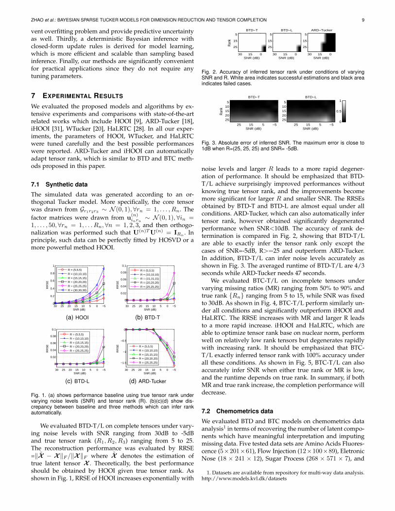
Fig. 1. (a) shows performance baseline using true tensor rank undervarying noise levels (SNR) and tensor rank (R). (b)(c)(d) show dis-crepancy between baseline and three methods which can infer rankautomatically.

We evaluated BTD-T/L on complete tensors under vary-ing noise levels with SNR ranging from 30dB to -5dBand true tensor rank (R1, R2, R3) ranging from 5 to 25.The reconstruction performance was evaluated by RRSE=‖X − X‖F /‖X‖F where X denotes the estimation oftrue latent tensor X . Theoretically, the best performanceshould be obtained by HOOI given true tensor rank. Asshown in Fig. 1, RRSE of HOOI increases exponentially with

SNR (dB)

Ran

k

BTD−T

30 15 0

5

15

25

SNR (dB)

BTD−L

30 15 0

5

15

25

SNR (dB)

ARD−Tucker

30 15 0

5

15

25

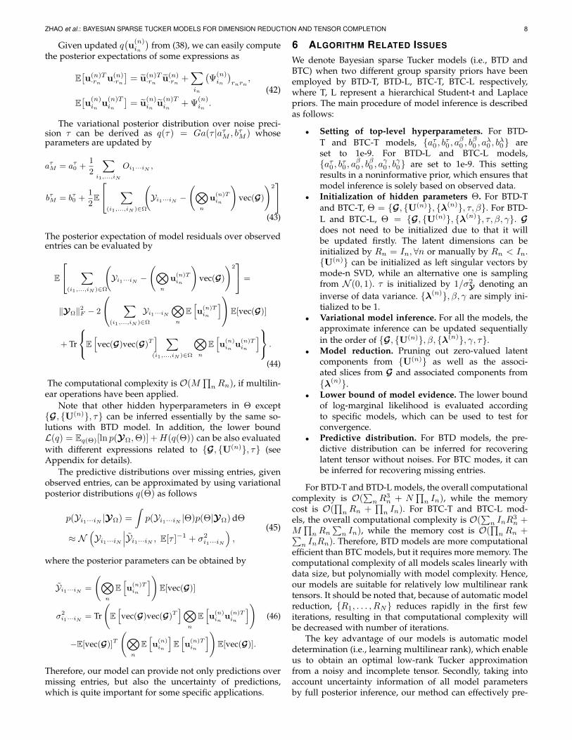
Fig. 2. Accuracy of inferred tensor rank under conditions of varyingSNR and R. White area indicates successful estimations and black areaindicates failed cases.

SNR (dB)

Ran

k

BTD−T

25 15 5 −5

510152025

SNR (dB)

BTD−L

25 15 5 −5

510152025

0

0.5

1

Fig. 3. Absolute error of inferred SNR. The maximum error is close to1dB when R=(25, 25, 25) and SNR= -5dB.

noise levels and larger R leads to a more rapid degener-ation of performance. It should be emphasized that BTD-T/L achieve surprisingly improved performances withoutknowing true tensor rank, and the improvements becomemore significant for larger R and smaller SNR. The RRSEsobtained by BTD-T and BTD-L are almost equal under allconditions. ARD-Tucker, which can also automatically infertensor rank, however obtained significantly degeneratedperformance when SNR<10dB. The accuracy of rank de-termination is compared in Fig. 2, showing that BTD-T/Lare able to exactly infer the tensor rank only except thecases of SNR=-5dB, R>=25 and outperform ARD-Tucker.In addition, BTD-T/L can infer noise levels accurately asshown in Fig. 3. The averaged runtime of BTD-T/L are 4/3seconds while ARD-Tucker needs 47 seconds.

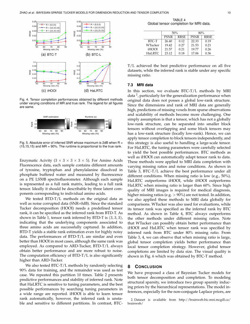
We evaluated BTC-T/L on incomplete tensors undervarying missing ratios (MR) ranging from 50% to 90% andtrue rank Rn ranging from 5 to 15, while SNR was fixedto 30dB. As shown in Fig. 4, BTC-T/L perform similarly un-der all conditions and significantly outperform iHOOI andHaLRTC. The RRSE increases with MR and larger R leadsto a more rapid increase. iHOOI and HaLRTC, which areable to optimize tensor rank base on nuclear norm, performwell on relatively low rank tensors but degenerates rapidlywith increasing rank. It should be emphasized that BTC-T/L exactly inferred tensor rank with 100% accuracy underall these conditions. As shown in Fig. 5, BTC-T/L can alsoaccurately infer SNR when either true rank or MR is low,and the runtime depends on true rank. In summary, if bothMR and true rank increase, the completion performance willdecrease.

7.2 Chemometrics data

We evaluated BTD and BTC models on chemometrics dataanalysis1 in terms of recovering the number of latent compo-nents which have meaningful interpretation and imputingmissing data. Five tested data sets are Amino Acids Fluores-cence (5×201×61), Flow Injection (12×100×89), EletronicNose (18 × 241 × 12), Sugar Process (268 × 571 × 7), and

1. Datasets are available from repository for multi-way data analysis.http://www.models.kvl.dk/datasets

http://www.models.kvl.dk/datasets


50 60 70 80 900

0.01

0.02

0.03

0.04

0.05

Missing ratio (%)

RR

SE

R = (5,5,5)R = (10,10,10)R = (15,15,15)

(a) BTC-T

50 60 70 80 900

0.01

0.02

0.03

0.04

0.05

Missing ratio (%)

RR

SE

R = (5,5,5)R = (10,10,10)R = (15,15,15)

(b) BTC-L

50 60 70 80 900

0.02

0.04

0.06

0.08

0.1

Missing ratio (%)

RR

SE

(c) iHOOI

50 60 70 80 900

0.2

0.4

0.6

0.8

1

Missing ratio (%)

RR

SE

(d) HaLRTC

Fig. 4. Tensor completion performances obtained by different methodsunder varying conditions of MR and true rank. The legend for all figuresare same.

Missing ratio (%)

Ran

k

SNR estimation

50 60 70 80 90

5

10

150

1

2

Missing ratio (%)

Ran

k

Runtime (s)

50 60 70 80 90

5

10

15 6080

100

Fig. 5. Absolute error of inferred SNR whose maximum is 2dB when R =(15,15,15) and MR = 90%. The runtime is proportional to the true rank.

Enzymatic Acivity (3 × 3 × 3 × 3 × 5). For Amino AcidsFluorescence data, each sample contains different amountsof tyrosine, tryptophan and phenylalanine dissolved inphosphate buffered water and measured by fluorescenceon a PE LS50B spectrofluorometer. Although each sampleis represented as a full rank matrix, leading to a full ranktensor. Ideally it should be describable by three latent com-ponents corresponding to individual amino acids.

We tested BTD-T/L methods on the original data aswell as noise corrupted data (SNR=0dB). Since the standardTucker decomposition (HOOI) needs a predefined tensorrank, it can be specified as the inferred rank from BTD-T. Asshown in Table 1, tensor rank inferred by BTD-T is (3, 3, 3),indicating that the underlying components associated tothree amino acids are successfully captured. In addition,BTD-T yields a stable rank estimation even for highly noisydata. The performances of BTD-T/L are similar and evenbetter than HOOI in most cases, although the same rank wasemployed. As compared to ARD-Tucker, BTD-T/L alwaysobtain better performance and are more robust to noise.The computation efficiency of BTD-T/L is also significantlyhigher than ARD-Tucker.

We also tested BTC-T/L methods by randomly selecting90% data for training, and the remainder was used as testcase. We repeated this partition 10 times. Table 2 presentspredictive performances and stability of inferred rank. Notethat HaLRTC is sensitive to tuning parameters, and the bestpossible performances by searching tuning parameters ina wide range are reported. iHOOI is able to learn tensorrank automatically, however, the inferred rank is unsta-ble and sensitive to different partitions. In contrast, BTC-

TABLE 4Global tensor completion for MRI data.

50% 80%PSNR RRSE PSNR RRSE

BTC-T 26.40 0.12 22.33 0.19WTucker 19.42 0.27 21.53 0.21iHOOI 21.57 0.21 19.77 0.26

HaLRTC 23.12 0.18 17.06 0.36

T/L achieved the best predictive performance on all fivedatasets, while the inferred rank is stable under any specificmissing ratio.

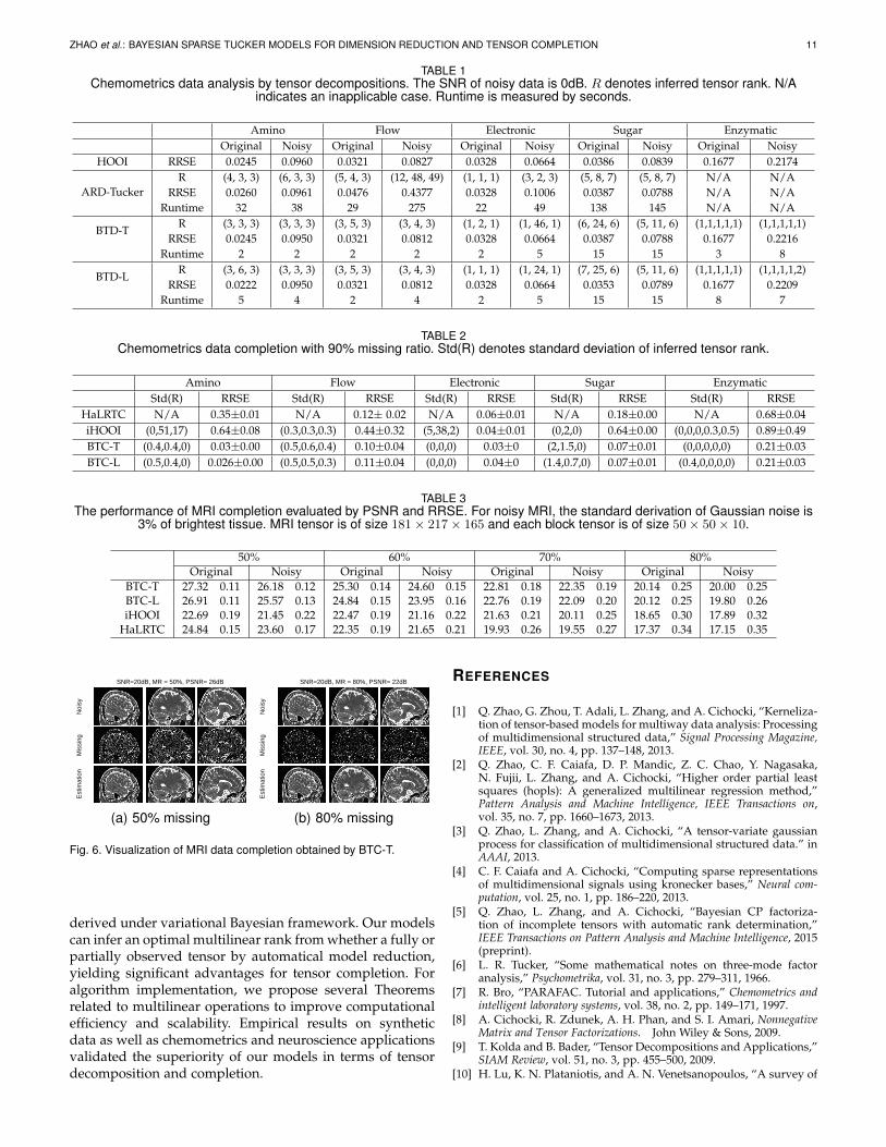
7.3 MRI dataIn this section, we evaluate BTC-T/L methods by MRIdata 2, particularly for the generalization performance whenoriginal data does not posses a global low-rank structure.Since the dimensions and rank of MRI data are generallyhigh, predictions of missing voxels from sparse observationsand scalability of methods become more challenging. Onesimply assumption is that a tensor, which has not a globallylow-rank structure, can be separated into smaller blocktensors without overlapping and some block tensors mayhas a low-rank structure (locally low-rank). Hence, we canapply tensor completion to block tensors independently, andthis strategy is also useful to handling a large-scale tensor.For HaLRTC, the tuning parameters were carefully selectedto yield the best possible performances. BTC methods aswell as iHOOI can automatically adapt tensor rank to data.These methods were applied to MRI data completion withvarying missing ratios and noise conditions. As shown inTable 3, BTC-T/L achieve the best performance under alldifferent conditions. When missing ratio is low (e.g., 50%),HaLRTC outperforms iHOOI, while iHOOI outperformsHaLRTC when missing ratio is larger than 60%. Since highquality of MRI images is required for medical diagnosis,higher missing ratios (e.g.> 90%) are not tested. In addition,we also applied these methods to MRI data globally forcomparisons. WTucker was also used for evaluations, whileits tensor rank was specified as the inferred rank by BTCmethod. As shown in Table 4, BTC always outperformsthe other methods under different missing ratios. Notethat WTucker can possibly obtain better performance thaniHOOI and HaLRTC when tensor rank was specified byinferred rank from BTC under 80% missing ratio. FromTable 3, 4, we can observe that when missing ratio is large,global tensor completion yields better performance thanlocal tensor completion strategy. However, global tensorcompletions are limited by data size. The visual quality isshown in Fig. 6 which was obtained by BTC-T method.

8 CONCLUSION

We have proposed a class of Bayesian Tucker models forboth tensor decomposition and completion. To modelingstructural sparsity, we introduce two group sparsity induc-ing priors by the hierarchical representations. The model in-ferences, especially for the non-conjugate Laplace priors, are

2. Dataset is available from http://brainweb.bic.mni.mcgill.ca/brainweb/

http://brainweb.bic.mni.mcgill.ca/brainweb/

http://brainweb.bic.mni.mcgill.ca/brainweb/


TABLE 1Chemometrics data analysis by tensor decompositions. The SNR of noisy data is 0dB. R denotes inferred tensor rank. N/A

indicates an inapplicable case. Runtime is measured by seconds.

Amino Flow Electronic Sugar EnzymaticOriginal Noisy Original Noisy Original Noisy Original Noisy Original Noisy

HOOI RRSE 0.0245 0.0960 0.0321 0.0827 0.0328 0.0664 0.0386 0.0839 0.1677 0.2174

ARD-TuckerR (4, 3, 3) (6, 3, 3) (5, 4, 3) (12, 48, 49) (1, 1, 1) (3, 2, 3) (5, 8, 7) (5, 8, 7) N/A N/A

RRSE 0.0260 0.0961 0.0476 0.4377 0.0328 0.1006 0.0387 0.0788 N/A N/ARuntime 32 38 29 275 22 49 138 145 N/A N/A

BTD-TR (3, 3, 3) (3, 3, 3) (3, 5, 3) (3, 4, 3) (1, 2, 1) (1, 46, 1) (6, 24, 6) (5, 11, 6) (1,1,1,1,1) (1,1,1,1,1)

RRSE 0.0245 0.0950 0.0321 0.0812 0.0328 0.0664 0.0387 0.0788 0.1677 0.2216Runtime 2 2 2 2 2 5 15 15 3 8

BTD-LR (3, 6, 3) (3, 3, 3) (3, 5, 3) (3, 4, 3) (1, 1, 1) (1, 24, 1) (7, 25, 6) (5, 11, 6) (1,1,1,1,1) (1,1,1,1,2)

RRSE 0.0222 0.0950 0.0321 0.0812 0.0328 0.0664 0.0353 0.0789 0.1677 0.2209Runtime 5 4 2 4 2 5 15 15 8 7

TABLE 2Chemometrics data completion with 90% missing ratio. Std(R) denotes standard deviation of inferred tensor rank.

Amino Flow Electronic Sugar EnzymaticStd(R) RRSE Std(R) RRSE Std(R) RRSE Std(R) RRSE Std(R) RRSE

HaLRTC N/A 0.35±0.01 N/A 0.12± 0.02 N/A 0.06±0.01 N/A 0.18±0.00 N/A 0.68±0.04iHOOI (0,51,17) 0.64±0.08 (0.3,0.3,0.3) 0.44±0.32 (5,38,2) 0.04±0.01 (0,2,0) 0.64±0.00 (0,0,0,0.3,0.5) 0.89±0.49BTC-T (0.4,0.4,0) 0.03±0.00 (0.5,0.6,0.4) 0.10±0.04 (0,0,0) 0.03±0 (2,1.5,0) 0.07±0.01 (0,0,0,0,0) 0.21±0.03BTC-L (0.5,0.4,0) 0.026±0.00 (0.5,0.5,0.3) 0.11±0.04 (0,0,0) 0.04±0 (1.4,0.7,0) 0.07±0.01 (0.4,0,0,0,0) 0.21±0.03

TABLE 3The performance of MRI completion evaluated by PSNR and RRSE. For noisy MRI, the standard derivation of Gaussian noise is

3% of brightest tissue. MRI tensor is of size 181× 217× 165 and each block tensor is of size 50× 50× 10.

50% 60% 70% 80%Original Noisy Original Noisy Original Noisy Original Noisy

BTC-T 27.32 0.11 26.18 0.12 25.30 0.14 24.60 0.15 22.81 0.18 22.35 0.19 20.14 0.25 20.00 0.25BTC-L 26.91 0.11 25.57 0.13 24.84 0.15 23.95 0.16 22.76 0.19 22.09 0.20 20.12 0.25 19.80 0.26iHOOI 22.69 0.19 21.45 0.22 22.47 0.19 21.16 0.22 21.63 0.21 20.11 0.25 18.65 0.30 17.89 0.32

HaLRTC 24.84 0.15 23.60 0.17 22.35 0.19 21.65 0.21 19.93 0.26 19.55 0.27 17.37 0.34 17.15 0.35

Noi

sy

SNR=20dB, MR = 50%, PSNR= 26dB

Mis

sing

Est

imat

ion

(a) 50% missing

Noi

sy

SNR=20dB, MR = 80%, PSNR= 22dB

Mis

sing

Est

imat

ion

(b) 80% missing

Fig. 6. Visualization of MRI data completion obtained by BTC-T.

derived under variational Bayesian framework. Our modelscan infer an optimal multilinear rank from whether a fully orpartially observed tensor by automatical model reduction,yielding significant advantages for tensor completion. Foralgorithm implementation, we propose several Theoremsrelated to multilinear operations to improve computationalefficiency and scalability. Empirical results on syntheticdata as well as chemometrics and neuroscience applicationsvalidated the superiority of our models in terms of tensordecomposition and completion.

REFERENCES

[1] Q. Zhao, G. Zhou, T. Adali, L. Zhang, and A. Cichocki, “Kerneliza-tion of tensor-based models for multiway data analysis: Processingof multidimensional structured data,” Signal Processing Magazine,IEEE, vol. 30, no. 4, pp. 137–148, 2013.

[2] Q. Zhao, C. F. Caiafa, D. P. Mandic, Z. C. Chao, Y. Nagasaka,N. Fujii, L. Zhang, and A. Cichocki, “Higher order partial leastsquares (hopls): A generalized multilinear regression method,”Pattern Analysis and Machine Intelligence, IEEE Transactions on,vol. 35, no. 7, pp. 1660–1673, 2013.

[3] Q. Zhao, L. Zhang, and A. Cichocki, “A tensor-variate gaussianprocess for classification of multidimensional structured data.” inAAAI, 2013.

[4] C. F. Caiafa and A. Cichocki, “Computing sparse representationsof multidimensional signals using kronecker bases,” Neural com-putation, vol. 25, no. 1, pp. 186–220, 2013.

[5] Q. Zhao, L. Zhang, and A. Cichocki, “Bayesian CP factoriza-tion of incomplete tensors with automatic rank determination,”IEEE Transactions on Pattern Analysis and Machine Intelligence, 2015(preprint).

[6] L. R. Tucker, “Some mathematical notes on three-mode factoranalysis,” Psychometrika, vol. 31, no. 3, pp. 279–311, 1966.

[7] R. Bro, “PARAFAC. Tutorial and applications,” Chemometrics andintelligent laboratory systems, vol. 38, no. 2, pp. 149–171, 1997.

[8] A. Cichocki, R. Zdunek, A. H. Phan, and S. I. Amari, NonnegativeMatrix and Tensor Factorizations. John Wiley & Sons, 2009.

[9] T. Kolda and B. Bader, “Tensor Decompositions and Applications,”SIAM Review, vol. 51, no. 3, pp. 455–500, 2009.

[10] H. Lu, K. N. Plataniotis, and A. N. Venetsanopoulos, “A survey of


multilinear subspace learning for tensor data,” Pattern Recognition,vol. 44, no. 7, pp. 1540–1551, 2011.

[11] V. De Silva and L.-H. Lim, “Tensor rank and the ill-posednessof the best low-rank approximation problem,” SIAM Journal onMatrix Analysis and Applications, vol. 30, no. 3, pp. 1084–1127, 2008.

[12] E. S. Allman, P. D. Jarvis, J. A. Rhodes, and J. G. Sumner, “Tensorrank, invariants, inequalities, and applications,” SIAM Journal onMatrix Analysis and Applications, vol. 34, no. 3, pp. 1014–1045, 2013.

[13] L.-H. Lim and C. Hillar, “Most tensor problems are NP hard,”University of California, Berkeley, 2009.

[14] M. Sørensen, L. De Lathauwer, P. COMON, S. ICART, andL. DENEIRE, “Canonical polyadic decomposition with orthogo-nality constraints,” SIAM Journal on Matrix Analysis and Applica-tions, no. accepted, 2012.

[15] L. Sorber, M. V. Barel, and L. D. Lathauwer, “Tensorlab v1.0,”Available online, URL: http://esat. kuleuven. be/sista/tensorlab, 2013.[Online]. Available: http://esat.kuleuven.be/sista/tensorlab/

[16] D. Tao, M. Song, X. Li, J. Shen, J. Sun, X. Wu, C. Faloutsos, andS. J. Maybank, “Bayesian tensor approach for 3-d face modeling,”Circuits and Systems for Video Technology, IEEE Transactions on,vol. 18, no. 10, pp. 1397–1410, 2008.

[17] S. Gao, L. Denoyer, P. Gallinari, and J. GUO, “Probabilistic latenttensor factorization model for link pattern prediction in multi-relational networks,” The Journal of China Universities of Posts andTelecommunications, vol. 19, pp. 172–181, 2012.

[18] M. Mørup and L. K. Hansen, “Automatic relevance determinationfor multi-way models,” Journal of Chemometrics, vol. 23, no. 7-8, pp.352–363, 2009.

[19] T. Yokota and A. Cichocki, “Multilinear tensor rank estimation viasparse tucker decomposition,” in Soft Computing and Intelligent Sys-tems (SCIS), 2014 Joint 7th International Conference on and AdvancedIntelligent Systems (ISIS), 15th International Symposium on. IEEE,2014, pp. 478–483.

[20] M. Filipovic and A. Jukic, “Tucker factorization with missing datawith application to low-n-rank tensor completion,” Multidimen-sional Systems and Signal Processing, pp. 1–16, 2013.

[21] W. Chu and Z. Ghahramani, “Probabilistic models for incompletemulti-dimensional arrays,” in JMLR Workshop and Conference Pro-ceedings Volume 5: AISTATS 2009, vol. 5, 2009, pp. 89–96.

[22] Z. Xu, F. Yan, and Y. Qi, “Bayesian nonparametric models formultiway data analysis,” Pattern Analysis and Machine Intelligence,IEEE Transactions on, vol. 37, no. 2, pp. 475–487, Feb 2015.

[23] L. Xiong, X. Chen, T.-K. Huang, J. Schneider, and J. G. Carbonell,“Temporal collaborative filtering with Bayesian probabilistic ten-sor factorization,” in Proceedings of SIAM Data Mining, vol. 2010,2010.

[24] E. Acar, D. M. Dunlavy, T. G. Kolda, and M. Mørup, “Scalable ten-sor factorizations for incomplete data,” Chemometrics and IntelligentLaboratory Systems, vol. 106, no. 1, pp. 41–56, 2011.

[25] K. Hayashi, T. Takenouchi, T. Shibata, Y. Kamiya, D. Kato, K. Ku-nieda, K. Yamada, and K. Ikeda, “Exponential family tensor fac-torization for missing-values prediction and anomaly detection,”in Data Mining (ICDM), 2010 IEEE 10th International Conference on.IEEE, 2010, pp. 216–225.

[26] P. Jain and S. Oh, “Provable tensor factorization with missingdata,” in Advances in Neural Information Processing Systems, 2014,pp. 1431–1439.

[27] P. Rai, Y. Wang, S. Guo, G. Chen, D. Dunson, and L. Carin,“Scalable bayesian low-rank decomposition of incomplete mul-tiway tensors,” in Proceedings of the 31st International Conference onMachine Learning (ICML-14), 2014, pp. 1800–1808.

[28] J. Liu, P. Musialski, P. Wonka, and J. Ye, “Tensor completion forestimating missing values in visual data,” IEEE Transactions onPattern Analysis and Machine Intelligence, vol. 35, no. 1, pp. 208–220, 2013.

[29] H. Tan, B. Cheng, W. Wang, Y.-J. Zhang, and B. Ran, “Tensorcompletion via a multi-linear low-n-rank factorization model,”Neurocomputing, vol. 133, pp. 161–169, 2014.

[30] H. Wang, F. Nie, and H. Huang, “Low-rank tensor completionwith spatio-temporal consistency,” in Twenty-Eighth AAAI Confer-ence on Artificial Intelligence, 2014.

[31] Y. Liu, F. Shang, W. Fan, J. Cheng, and H. Cheng, “Generalizedhigher-order orthogonal iteration for tensor decomposition andcompletion,” in Advances in Neural Information Processing Systems,2014, pp. 1763–1771.

[32] Y. Liu, F. Shang, H. Cheng, J. Cheng, and H. Tong, “Factormatrix trace norm minimization for low-rank tensor completion,”

in Proceedings of the 2014 SIAM International Conference on DataMining, 2014.

[33] M. Signoretto, Q. T. Dinh, L. De Lathauwer, and J. A. Suykens,“Learning with tensors: a framework based on convex optimiza-tion and spectral regularization,” Machine Learning, pp. 1–49, 2013.

[34] D. Kressner, M. Steinlechner, and B. Vandereycken, “Low-ranktensor completion by riemannian optimization,” BIT NumericalMathematics, pp. 1–22, 2013.

[35] Y.-L. Chen, C.-T. Hsu, and H.-Y. Liao, “Simultaneous tensor de-composition and completion using factor priors,” IEEE Transac-tions on Pattern Analysis and Machine Intelligence, vol. 36, no. 3, pp.577–591, 2014.

[36] A. Narita, K. Hayashi, R. Tomioka, and H. Kashima, “Tensorfactorization using auxiliary information,” Data Mining and Knowl-edge Discovery, vol. 25, no. 2, pp. 298–324, 2012.

[37] M. E. Tipping, “Sparse Bayesian learning and the relevance vectormachine,” The Journal of Machine Learning Research, vol. 1, pp. 211–244, 2001.

[38] S. D. Babacan, M. Luessi, R. Molina, and A. K. Katsaggelos,“Sparse Bayesian methods for low-rank matrix estimation,” IEEETransactions on Signal Processing, vol. 60, no. 8, pp. 3964–3977, 2012.

[39] C. Bishop, “Variational principal components,” in Artificial NeuralNetworks, 1999. ICANN 99. Ninth International Conference on (Conf.Publ. No. 470), vol. 1. IET, 1999, pp. 509–514.

[40] M. A. Figueiredo, “Adaptive sparseness for supervised learning,”Pattern Analysis and Machine Intelligence, IEEE Transactions on,vol. 25, no. 9, pp. 1150–1159, 2003.

[41] S. D. Babacan, R. Molina, and A. K. Katsaggelos, “Bayesiancompressive sensing using laplace priors,” Image Processing, IEEETransactions on, vol. 19, no. 1, pp. 53–63, 2010.

[42] S. D. BABACAN, S. NAKAJIMA, and M. N. DO, “Bayesian group-sparse modeling and variational inference,” IEEE transactions onsignal processing, vol. 62, no. 9-12, pp. 2906–2921, 2014.

[43] J. M. Winn and C. M. Bishop, “Variational message passing,”Journal of Machine Learning Research, vol. 6, pp. 661–694, 2005.

Qibin Zhao received the Ph.D. degree from De-partment of Computer Science and Engineering,Shanghai Jiao Tong University, Shanghai, China,in 2009. He is currently a research scientistat Laboratory for Advanced Brain Signal Pro-cessing in RIKEN Brain Science Institute, Japanand is also a visiting professor in Saitama Insti-tute of Technology, Japan. His research interestsinclude machine learning, tensor factorization,computer vision and brain computer interface.He has published more than 50 papers in inter-

national journals and conferences.

Liqing Zhang received the Ph.D. degree fromZhongshan University, Guangzhou, China, in1988. He is now a Professor with Department ofComputer Science and Engineering, ShanghaiJiao Tong University, Shanghai, China. His cur-rent research interests cover computational the-ory for cortical networks, visual perception andcomputational cognition, statistical learning andinference. He has published more than 210 pa-pers in international journals and conferences.

http://esat.kuleuven.be/sista/tensorlab/


Andrzej Cichocki received the Ph.D. and Dr.Sc.(Habilitation) degrees, all in electrical engi-neering, from Warsaw University of Technology(Poland). He is the senior team leader of theLaboratory for Advanced Brain Signal Process-ing, at RIKEN BSI (Japan). He is coauthor ofmore than 400 scientific papers and 4 mono-graphs (two of them translated to Chinese). Heserved as AE of IEEE Trans. on Signal Process-ing, TNNLS, Cybernetics and J. of NeuroscienceMethods.

Documents

PDF - arXiv.org e-Print archive · ZHAO et al.: BAYESIAN SPARSE TUCKER MODELS FOR DIMENSION REDUCTION AND TENSOR COMPLETION 2 tion performance, whereas this problem is …