Y1-DES mocks 1

FERMILAB-PUB-17-587

DES-2017-0292

IFT-UAM/CSIC-17-124

Dark Energy Survey Year 1 Results: galaxy mockcatalogues for BAO

S. Avila1,2,3?, M. Crocce4, A. J. Ross5, J. Garcıa-Bellido2,3, W. J. Percival1, N. Banik6,7,8,9,H. Camacho10,11, N. Kokron10,11,12,13, K. C. Chan4,14, F. Andrade-Oliveira11,15, R. Gomes10,11, D.Gomes10,11, M. Lima10,11, R. Rosenfeld11,12, O. Friedrich16,17, F. B. Abdalla18,19, J. Annis7, A. Benoit-Levy18,20,21, E. Bertin20,21, D. Brooks18, M. Carrasco Kind22,23, J. Carretero24, F. J. Castander4,C. E. Cunha25, L. N. da Costa11,26, C. Davis25, J. De Vicente27, P. Doel18, P. Fosalba4, J. Frieman7,28,D. W. Gerdes29,30, D. Gruen25,31, R. A. Gruendl22,23, G. Gutierrez7, W. G. Hartley18,32,D. Hollowood33, K. Honscheid5,34, D. J. James35, K. Kuehn36, N. Kuropatkin7, R. Miquel24,37,A. A. Plazas38, E. Sanchez27, V. Scarpine7, R. Schindler31, M. Schubnell30, I. Sevilla-Noarbe27,M. Smith39, F. Sobreira11,40, E. Suchyta41, M. E. C. Swanson23, G. Tarle30, D. Thomas1,A. R. Walker42

(The Dark Energy Survey Collaboration)

1 Institute of Cosmology & Gravitation, Dennis Sciama Building, University of Portsmouth, Portsmouth, PO1 3FX, UK2 Departamento de Fısica Teorica, Modulo C-15, Facultad de Ciencias, Universidad Autonoma de Madrid, 28049 Cantoblanco, Madrid, Spain3 Instituto de Fısica Teorica, UAM-CSIC, Universidad Autonoma de Madrid, 28049 Cantoblanco, Madrid, Spain4 Institut de Ciencies de l’Espai, IEEC-CSIC, Campus UAB, Facultat de Ciencies, Torre C5 par-2, Barcelona 08193, Spain5 Center for Cosmology and AstroParticle Physics, The Ohio State University, Columbus, OH 43210, USA6 Department of Physics, University of Florida, Gainesville, Florida 32611, USA7 Fermi National Accelerator Laboratory, Batavia, Illinois 60510, USA8 GRAPPA, Institute of Theoretical Physics, University of Amsterdam, Science Park 904, 1090 GL Amsterdam9 Lorentz Institute, Leiden University, Niels Bohrweg 2, Leiden, NL-2333 CA, The Netherlands10 Departamento de Fısica Matematica, Instituto de Fısica, Universidade de Sao Paulo,CP 66318, Sao Paulo, SP, 05314-970, Brazil11 Laboratorio Interinstitucional de e-Astronomia, Rua General Jose Cristino, 77, Sao Cristovao, Rio de Janeiro, RJ, 20921-400, Brazil12 ICTP South American Institute for Fundamental Research & Instituto de Fısica Teorica, Universidade Estadual Paulista, Sao Paulo, Brazil13 Department of Physics, Stanford University, 382 Via Pueblo Mall, Stanford, CA 94305, USA14 School of Physics and Astronomy, Sun Yat-Sen University, Guangzhou 510275, China15 Instituto de Fısica Teorica, Universidade Estadual Paulista, Sao Paulo, Brazil16 Max Planck Institute for Extraterrestrial Physics, Giessenbachstrasse, 85748 Garching, Germany17 Universitats-Sternwarte, Fakultat fur Physik, Ludwig-Maximilians Universitat Munchen, Scheinerstr. 1, 81679 Munchen, Germany18 Department of Physics & Astronomy, University College London, Gower Street, London, WC1E 6BT, UK19 Department of Physics and Electronics, Rhodes University, PO Box 94, Grahamstown, 6140, South Africa20 CNRS, UMR 7095, Institut d’Astrophysique de Paris, F-75014, Paris, France21 Sorbonne Universites, UPMC Univ Paris 06, UMR 7095, Institut d’Astrophysique de Paris, F-75014, Paris, France22 Department of Astronomy, University of Illinois, 1002 W. Green Street, Urbana, IL 61801, USA23 National Center for Supercomputing Applications, 1205 West Clark St., Urbana, IL 61801, USA24 Institut de Fısica d’Altes Energies (IFAE), The Barcelona Institute of Science and Technology, Campus UAB, 08193 Bellaterra (Barcelona) Spain25 Kavli Institute for Particle Astrophysics & Cosmology, P. O. Box 2450, Stanford University, Stanford, CA 94305, USA26 Observatorio Nacional, Rua Gal. Jose Cristino 77, Rio de Janeiro, RJ - 20921-400, Brazil27 Centro de Investigaciones Energeticas, Medioambientales y Tecnologicas (CIEMAT), Madrid, Spain28 Kavli Institute for Cosmological Physics, University of Chicago, Chicago, IL 60637, USA29 Department of Astronomy, University of Michigan, Ann Arbor, MI 48109, USA30 Department of Physics, University of Michigan, Ann Arbor, MI 48109, USA31 SLAC National Accelerator Laboratory, Menlo Park, CA 94025, USA32 Department of Physics, ETH Zurich, Wolfgang-Pauli-Strasse 16, CH-8093 Zurich, Switzerland33 Santa Cruz Institute for Particle Physics, Santa Cruz, CA 95064, USA34 Department of Physics, The Ohio State University, Columbus, OH 43210, USA35 Astronomy Department, University of Washington, Box 351580, Seattle, WA 98195, USA36 Australian Astronomical Observatory, North Ryde, NSW 2113, Australia37 Institucio Catalana de Recerca i Estudis Avancats, E-08010 Barcelona, Spain38 Jet Propulsion Laboratory, California Institute of Technology, 4800 Oak Grove Dr., Pasadena, CA 91109, USA39 School of Physics and Astronomy, University of Southampton, Southampton, SO17 1BJ, UK40 Instituto de Fısica Gleb Wataghin, Universidade Estadual de Campinas, 13083-859, Campinas, SP, Brazil41 Computer Science and Mathematics Division, Oak Ridge National Laboratory, Oak Ridge, TN 3783142 Cerro Tololo Inter-American Observatory, National Optical Astronomy Observatory, Casilla 603, La Serena, Chile

19 December 2017

c© 2017 RAS, MNRAS 0000, 2–18

arX

iv:1

712.

0623

2v1

[as

tro-

ph.C

O]

18

Dec

201

7

Mon. Not. R. Astron. Soc. 0000, 2–18 (2017) Printed 19 December 2017 (MN LATEX style file v2.2)

ABSTRACTMock catalogues are a crucial tool in the analysis of galaxy surveys data, both forthe accurate computation of covariance matrices, and for the optimisation of analy-sis methodology and validation of data sets. In this paper, we present a set of 1800galaxy mock catalogues designed to match the Dark Energy Survey Year-1 BAO sam-ple (Crocce et al. 2017) in abundance, observational volume, redshift distribution anduncertainty, and redshift dependent clustering. The simulated samples were built uponhalogen (Avila et al. 2015) halo catalogues, based on a 2LPT density field with anexponential bias. For each of them, a lightcone is constructed by the superposition ofsnapshots in the redshift range 0.45 < z < 1.4. Uncertainties introduced by so-calledphotometric redshifts estimators were modelled with a double-skewed-Gaussian curvefitted to the data. We also introduce a hybrid HOD-HAM model with two free pa-rameters that are adjusted to achieve a galaxy bias evolution b(zph) that matches thedata at the 1-σ level in the range 0.6 < zph < 1.0. We further analyse the galaxymock catalogues and compare their clustering to the data using the angular correla-tion function w(θ), the comoving transverse separation clustering ξµ<0.8(s⊥) and theangular power spectrum C`.

Key words: methods: numerical – large-scale structure of Universe – cosmology:theory

1 INTRODUCTION

The Large Scale Structure (LSS) of the Universe has provento be a very powerful tool to study Cosmology. In particular,distance measurements of the Baryonic Acoustic Oscillation(BAO) scale (Peebles & Yu 1970; Sunyaev & Zeldovich 1970)can be used to infer the expansion history of the Universeand, hence, to constrain dark energy properties. Whereasmost BAO detections have been performed by spectroscopicgalaxy surveys, able to estimate radial positions with greataccuracy (Cole et al. 2005; Eisenstein et al. 2005; Beut-ler et al. 2011; Blake et al. 2011; Ross et al. 2017b; Ataet al. 2017), the size and depth of the Dark Energy Survey1

(DES) gives us the opportunity to measure the BAO angu-lar distance DA(z) with competing constraining power usingonly photometry. Photometric galaxy surveys provide mod-erately accurate estimates of the redshift of galaxies fromthe magnitudes observed through a number of filters (5, inthe case of DES) (Hoyle et al. 2017), making it more dif-ficult to obtain BAO measurements. However, the fidelitywith which the BAO is observed is boosted by the photo-metric survey’s capability to explore larger areas of the sky(1318 deg2 for the BAO DES sample from data taken in thefirst year, ∼ 5000 deg2 for the complete survey) and largernumber of galaxies (∼ 300 million for the complete DES).The current Year-1 (Y1) DES data already allow us to probea range 0.6 < z < 1 poorly explored with BAO physics.

This paper is released within a series of studies devotedto the measurement of the BAO scale with the DES Y1 data.The main results are presented in DES Collaboration (2017)(here after DES-BAO-MAIN), including a ∼ 4% precisionDA BAO measurement. Crocce et al. (2017) defines the sam-ple selection optimised for BAO analysis (hereafter DES-BAO-SAMPLE). A photometric redshift validation over thesample is performed in Gaztanaga et al. (in preparation)

? e-mail: santiagoavilaperez@gmail.com1 www.darkenergysurvey.org

(hereafter DES-BAO-PHOTOZ). A method to extract theBAO from angular clustering in tomographic redshift binsis presented in Chan et al. (in preparation) (from nowDES-BAO-θ-METHOD). Ross et al. (2017a) (DES-BAO-s⊥-METHOD in the remainder) explains a method to ex-tract the BAO information from the comoving transversedistace clustering. Camacho et al (in preparation) (DES-BAO-`-METHOD from now), presents a method to extractthe BAO scale from the angular power spectrum. This paperwill be devoted to the simulations used in the analysis.

In order to analyse the data we need an adequate the-oretical framework. Even though there are analytic modelsthat can help us understand the structure formation of theUniverse (Press & Schechter 1974; Kaiser 1984; Bond et al.1991; Cooray & Sheth 2002; Zel’dovich 1970; Kaiser 1987;Moutarde et al. 1991), most realistic models are based onnumerical simulations. Simulations have the additional ad-vantages that they allow us to easily include observationaleffects such as masks and redshift uncertainties and can real-istically mimic how these couple with other sources of uncer-tainty such as cosmic variance or shot noise. For the estima-tion of the covariance matrices of our measurements we needa number of the order of hundreds to thousands of simula-tions, depending on the size of the data vector analysed (Do-delson & Schneider 2013), in order that the uncertainty inthe covariance matrices is subdominant for the final results.As full N -Body simulations require considerable computingresources, running that number of N -Body simulations isunfeasible. Since we will only be interested in large scales,approximate mock catalogues are a good alternative to sim-ulate our data set in a much more computationally efficientway (Bond & Myers 1996; Scoccimarro & Sheth 2002; Man-era et al. 2013; Kitaura et al. 2016; Chuang et al. 2015a;Avila et al. 2015; Tassev et al. 2013; Monaco et al. 2013;White et al. 2014; Chuang et al. 2015b; Monaco 2016). Al-ternatively, we can use a lower number of mock cataloguescombining them with theory using hybrid methods (Pope &Szapudi 2008; Taylor & Joachimi 2014; Scoccimarro 2000;

c© 2017 RAS

Y1-DES mocks 3

Friedrich & Eifler 2017), this possibility is explored in a com-panion paper (DES-BAO-θ-METHOD).

Galaxy mock catalogues are important in Large ScaleStructure studies not only for the computation of covariancematrices, but also crucial when optimising the methodol-ogy and understanding the significance of any particularityfound in the data itself, and learn how to interpret/deal withit (see, for example, Appendix A in DES-BAO-MAIN).

The main properties from the simulations that we needto match to the data in order to correctly reproduce the co-variance are: the galaxy abundance, the galaxy bias evolu-tion, the redshift uncertainties and the shape of the sampledvolume (angular mask and redshift range). In this paper wepresent a set of 1800 mock catalogues designed to statisti-cally match those properties of the DES Y1-BAO sample.The definition of that sample is summarised in Section 2.As a first step, we use the halo generator method calledhalogen (Avila et al. 2015, summarised in Section 3.1),to create dark matter halo catalogues in Cartesian coordi-nates and fixed redshift. We then generate a lightcone (Sec-tion 3.2) by transforming our catalogues to observationalcoordinates ra, dec, zsp, accounting for redshift evolution,and implement the survey mask (Section 3.3). In Section 4we model and implement the redshift uncertainties intro-duced in the sample by the photometric redshift techniques.The galaxy clustering model is described in Section 5, wherewe introduce a redshift evolving hybrid Halo OccupationDistribution (HOD) - Halo Abundance Matching (HAM)model. Finally, in Section 6 we analyse the set of mock cat-alogues, comparing their covariance matrices with the the-oretical model in DES-BAO-θ-METHOD, and we comparethe clustering measurements in angular configuration space(wi(θ)), three-dimensional configuration space (ξ<µ0.8(s⊥))and angular harmonic space (Cil ) of our mock catalogueswith the data and theoretical models. We conclude in Sec-tion 7.

2 THE REFERENCE DATA

The aim of this paper is to reproduce in a cosmological sim-ulation all the properties relevant for BAO analysis of theDES Y1-BAO sample. We describe how this sample is se-lected below in Section 2.1, and how the redshifts of thatsample are obtained in Section 2.2. We also describe how wecompute correlation functions from data or simulations inSection 2.3.

2.1 The Y1-BAO Sample

The Y1-BAO sample is a subsample of the Gold Catalogue(Drlica-Wagner et al. 2017) obtained from the first Year ofDES observations (Diehl et al. 2014). The Gold Catalogueprovides ‘clean’ galaxy catalogues and photometry as de-scribed in Drlica-Wagner et al. (2017). A footprint quantifiedusing a Healpix (Gorski et al. 2005) map with nside = 4096is provided with all the areas with at least 90s of exposuretime in all the filters g,r,i and z, summing up to ∼ 1800deg2.After vetoing bright stars and the Large Magellanic Cloud,the area is reduced to ∼ 1500deg2.

The Y1-BAO sample selection procedure was optimisedto obtain precise BAO measurements at high redshift and

is fully described in (DES-BAO-SAMPLE). The Y1-BAOsample is obtained applying three main selection criteria:

17.5 < iauto < 19.0 + 3.0 zBPZ−MA

(iauto − zauto) + 2.0(rauto − iauto) > 1.7

0.6 < zph < 1.0

(1)

with Xauto being the mag auto magnitude in the band X,and zBPZ−MA the photometric redshift obtained by BPZ(Benıtez 2000) using mag auto photometry, and zph be-ing the photometric redshift (either zBPZ−MA or zDNF−MOF

see below). Apart from the three main cuts in Equation 1,we remove outliers in color space and perform a star-galaxyseparation. Further veto masks are applied to the Y1-BAOsample guaranteeing at least a 80% coverage in the fourbands, requiring sufficient depth-limit in different bands andremoving ‘bad regions’. The final Y1-BAO sample after allthe veto masks have been applied covers an effective area of1318 deg2 (see more details in DES-BAO-SAMPLE).

2.2 Photometric redshifts

The redshift estimation for each galaxy is based on themagnitude observed in each filter. For this paper, we willuse two combinations of photometry and photo-z code, re-spectively: mag auto with BPZ (BPZ-MA), and MOF withDNF (DNF-MOF). A description on how the two photome-try techniques extract the magnitude from the image can befound in Drlica-Wagner et al. (2017). A thorough descrip-tion and comparison of both photometric redshift methodsutilised here can be found in Hoyle et al. (2017). First, wehave BPZ (Bayesian Photometric Redshift, Benıtez 2000;Benıtez et al. 2004), which is a method based on synthetictemplates of spectra convolved with the DES filters, andmakes use of Bayesian inference. On the other hand, wehave DNF (Directional Neighbourhood Fitting, De Vicenteet al. 2016), which is a training-based method.

Both methods take the results from the chosen photom-etry in the four bands and give a Probability-Distribution-Function (PDF) for the redshift of each galaxy: P (z). As afull PDF for each galaxy would build up a very large datasetto transfer and work with, here we take two quantities fromeach PDF: the mean zph ≡ 〈P (z)〉, and a random draw fromthe distribution zmc. We will explain in Section 4 how we willmodel the effect of photometric redshift in our simulations.

By default, the reference data will use the DNF-MOFredshift zDNF−MOF, since this is the one used in DES-BAO-MAIN for the fiducial results. We will only include zBPZ−MA

in Section 4, since it was the reference redshift when part ofthe methodology presented in that section was designed.

2.3 2-point Correlation Functions

Throughout this paper we analyse 2-point correlation func-tions in repeated occasions. In all cases we use the Landy-Szalay estimator (Landy & Szalay 1993):

Ψ(x) =DD(x)− 2DR(x) +RR(x)

RR(x)(2)

c© 2017 RAS, MNRAS 0000, 2–18

4 Avila et al.

with DD, DR and RR being respectively the number ofData-Data, Data-Random and Random-Random pairs sep-arated by a distance x. The correlation Ψ refers to either anangular correlation denoted by w, or a three-dimensionalcorrelation ξ. The variable x may correspond to the an-gular separation θ projected on to the sky, or the three-dimensional comoving separation r. In the three-dimensionalcase, we will sometimes study the anisotropic correlation,distinguishing between the distance parallel to the line-of-sight and perpendicular to it, having x = s‖, s⊥.

The data D may refer to observed data or simulateddata. Random catalogues R are produced by populating thesame sampled volume as the data with randomly distributedpoints. All the correlation function presented here were com-puted with the public code cute (Alonso 2012)2.

3 HALO LIGHTCONE CATALOGUES

Prior to the generation of the galaxy catalogues, we needto construct the field of dark matter halos. For this, we willuse the technique called halogen, a technique that pro-duces halo catalogues with Cartesian coordinates embeddedin a cube and at a given time slice (snapshot). By super-posing a series of halogen snapshots, we construct an ob-servational catalogue with angular coordinates and redshiftra,dec,zsp: a lightcone halo catalogue. Finally, we describehow we implement the survey mask in the mock cataloguesin order to statistically reproduce the angular distributionof the data.

3.1 HALOGEN

halogen3 (described in Avila et al. 2015 and compared withother methods in Chuang et al. 2015b) is a fast approximatemethod to generate halo mock catalogues.

It consists of 4 major steps:

(i) Generate a distribution of particles with 2nd-orderPerturbation Theory (Moutarde et al. 1991; Bouchet et al.1995, 2LPT) at fixed redshift. Distribute those particles incells of size lcell

(ii) Produce a list of halo masses Mh from a theoreti-cal/empirical Halo Mass Function (HMF).

(iii) Place the halos at the position of particles with aprobability dependent on the cell density and halo mass asPcell ∝ ρ

α(Mh)cell . An exclusion criterion is imposed to avoid

halo overlap and we ensure that the total mass of the halosdoes not exceed the total amount of matter in that cell.

(iv) Assign the velocities of the particles to the halosrescaled through a factor: vhalo = fvel(Mh) · vpart

There are one parameter, and two functions of halomass that have been introduced in the method and need toto be set for each run. We set the cell size lcell = 5h−1Mpcas in Avila et al. (2015). The parameter α(Mh) is fitted to areference N -Body simulation to match the mass-dependentclustering and the factor fvel(Mh) is also calibrated againstan N -Body simulation in order to reproduce the velocity

2 https://github.com/damonge/CUTE3 https://github.com/savila/HALOGEN

10

100

1000

r2 ξ

(r)

z=0.0

HALOGENMICE

z=0.5

[Mpc/h]

10

100

1000

0 20 40 60 80 100 120 140

r2 ξ

(r)

r

z=1.0

[Mpc/h]

Mth= 1 1013

Mth= 5 1012

Mth=2.5 1012

0 20 40 60 80 100 120 140r

z=1.5

[Mpc/h]

Mth=1.6 1014

Mth= 8 1013

Mth= 4 1013

Mth= 2 1013

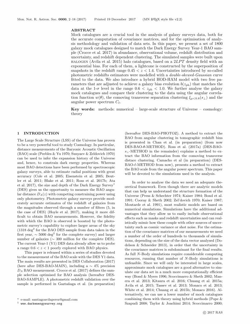
Figure 1. 2-point correlation function of mice vs. halogen halosin the simulation box at the snapshots z = 0.0, 0.5, 1.0 and 1.5

as labelled. We display the different mass thresholds Mth used

during the fit (finding higher correlations for higher Mth).

distributions. For this study we use the mice simulation asa reference for this calibration.

The MICE Grand Challenge simulation, described in(Fosalba et al. 2015a; Crocce et al. 2015; Fosalba et al.2015b), is based on a cosmology with parameters: ΩM =0.25, ΩΛ = 0.75, Ωb = 0.044, h = 0.7, σ8 = 0.8, ns = 0.95matching early WMAP data (Hinshaw et al. 2007). We willuse this fiducial cosmology throughout the paper. The boxsize of the simulation is Lbox = 3072h−1Mpc and made useof 40963 particles. The halogen catalogues use a lower massresolution with 12803 particles in order to reduce the re-quired computing resources. We use the same box size andcosmology for halogen.

For the calibration we used the same phases of the initialconditions as the N -Body simulation and fitted the halo-gen parameters with the snapshots at zsnap = 0, 0.5, 1.0, 1.5.We input to halogen a hybrid Halo Mass Function, usingthe HMF directly measured from mice catalogues at lowmasses, while using an analytic expression (Watson et al.2013) generated with hmfcalc4 (Murray et al. 2013) forthe large masses, where the HMF from the mice cataloguesare noise dominated.

We fitted the clustering of the halos in logarithmic massbins (with factor 2 in mass threshold), this being a slightvariation with respect to the method used in Avila et al.(2015). The minimum halo mass that we probe is Mh =2.5 × 1012M/h for snaphots at z 6 1.0, whereas we use aminimum mass of Mh = 5.0× 1012M/h for higher redshiftsnaphots. Once the parameter calibration is finished, we finda good agreement between mice and halogen correlationfunctions as a function of redshift and mass, as shown inFigure 1.

3.2 Lightcone

We place the observer at the origin (i.e., one corner ofthe box), so that we can simulate one octant of the sky,

4 http://hmf.icrar.org

c© 2017 RAS, MNRAS 0000, 2–18

Y1-DES mocks 5

and transform to spherical coordinates. We use the nota-tion zsp for the redshift of a halo or galaxy as it would beobserved with a spectroscopic survey (i.e., with negligibleuncertainty). We have that

zsp = z(r) +1 + z(r)

c~u · r , (3)

with ~r = X,Y, Z the comoving position, ~u the comovingvelocity, r = |~r|, r = ~r/r and z(r) the inverse of

r(z) = c

∫ z

0

dz′

H(z′). (4)

The first term in Equation 3 corresponds to the redshiftdue to the Hubble expansion, whereas the second term is thecontribution from the peculiar velocity of the galaxy.

Given the redshift range covered by DES, we need toallow for redshift-dependent clustering, and hence we willlet the halogen parameters (α, fvel, and the HMF) vary asa function of redshift.

The halogen parameters, obtained by fitting the micesimulation (Section 3.1) at zsnap = 0, 0.5, 1, 1.5, were inter-polated to zsnap,i = 0.3, 0.55, 0.625, 0.675, 0.725, 0.775,0.825, 0.875, 0.925, 0.975, 1.05 and 1.3, then halogen wasrun at those redshifts. We build the lightcone from the su-perposition of spherical zsp-shells drawn from the snapshotsby setting the edges at the intermediate redshifts. So eachsnapshot i contributes galaxies whose redshift is in the in-terval zsp ∈ [

zsnap,i−1+zsnap,i

2,zsnap,i+zsnap,i+1

2], also impos-

ing the edges of the lightcone at zsp = 0.1 and zsp = 1.42(which is the maximum redshift reachable given the chosengeometry and cosmology). A priori, there will be a relativelysharp transition of the clustering properties at the edges ofthe zsp-shells, but, once we have introduced the redshift un-certainties in Section 4, those transitions will be smoothed.Throughout Sections 3,4,5 we will focus the analysis in 8photometric redshift bins with width ∆zph = 0.05 betweenzph = 0.6 and zph = 1.0. When dealing with true redshiftspace, we will need to extend the boundaries to the range0.45 < zsp < 1.4 (see Section 4).

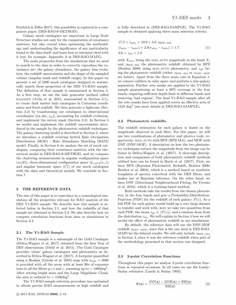
Finally, we compare the resulting halogen lightconewith the halo lightcone generated by mice in Figure 2. Notethat the mice simulated lightcone is constructed from finetimeslices (∆z = 0.005 − 0.025) built on-the-fly from a fullN -Body simulation and using the velocity of the particles toextrapolate their positions at the precise moment they crossthe lightcone (Fosalba et al. 2008). Remarkably, despite thelarge differences in the methodology, the angular correla-tion functions from both lightcones show very good agree-ment at all redshifts, independently of whether the halogenparameters were fitted or interpolated. At large scales sam-pling variance becomes dominant, modifying stochasticallythe shape of the correlation function, but since we imposedthe same phases of the initial conditions, it enables us tomake a one-to-one comparison.

3.3 Angular selection

In Section 3.2 we placed the observer at one corner, pro-viding a sample covering an octant of the sky. In Section 2

0.0001

0.001

0.01

0.1

w(θ

)

0.475<z<0.525

MICE HALOGEN

0.0001

0.001

0.01

0.1

w(θ

)

0.60<z<0.65

0.0001

0.001

0.01

0.1

0.2 0.5 1.0 2.0 5.0

w(θ

)

θ(°)

0.70<z<0.75

0.80<z<0.85

0.90<z<0.95

0.2 0.5 1.0 2.0 5.0

θ(°)

0.975<z<1.025

Figure 2. Angular correlation function of halos from the mice

(crosses) and halogen (lines) lightcones. The different panelscorrespond to different redshift bins, as labelled, with width

∆zsp = 0.05. We mark in solid lines the redshifts at which halo-

gen parameters were fitted, and in dashed lines results from in-terpolated parameters. Correlation functions shown correspond

to mass cuts at Mh = 2.5× 1012M/h .

we described how, we obtained a footprint covering the ef-fectively observed area of the sky. This mask spreads overa large fraction of the sky and cannot be fit into a singleoctant. However, using the periodic boundary conditions ofthe box, we can put 8 replicas of the box together to build alarger cube, and extract a full sky lightcone catalogue, albeitwith a repeating pattern of galaxies.

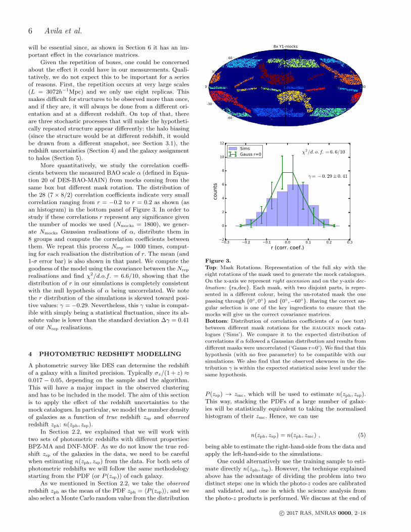
In the top panel of Figure 3 we show how we can draw 8mock catalogues with the Y1 footprint from the full sky cata-logue by performing rotations on the sphere. We see that thefootprint has a complicated shape with two disjoint areas:one passing by ra = 0, dec = 0 known as Stripe-82 (thatoverlaps with many other surveys), and another passing byra = 0, dec = −60, known as SPT-region (due to theoverlap with the South Pole Telescope observations). Whiledesigning the rotations depicted in Figure 3, we made surethat every pair of footprints would not overlap and that thetwo disjoint areas are separated by more than the maximumscale of interest (∼ 6, see Section 6.2).

Including this angular selection to the mock catalogues

c© 2017 RAS, MNRAS 0000, 2–18

6 Avila et al.

will be essential since, as shown in Section 6 it has an im-portant effect in the covariance matrices.

Given the repetition of boxes, one could be concernedabout the effect it could have in our measurements. Quali-tatively, we do not expect this to be important for a seriesof reasons. First, the repetition occurs at very large scales(L = 3072h−1Mpc) and we only use eight replicas. Thismakes difficult for structures to be observed more than once,and if they are, it will always be done from a different ori-entation and at a different redshift. On top of that, thereare three stochastic processes that will make the hypotheti-cally repeated structure appear differently: the halo biasing(since the structure would be at different redshift, it wouldbe drawn from a different snapshot, see Section 3.1), theredshift uncertainties (Section 4) and the galaxy assignmentto halos (Section 5).

More quantitatively, we study the correlation coeffi-cients between the measured BAO scale α (defined in Equa-tion 20 of DES-BAO-MAIN) from mocks coming from thesame box but different mask rotation. The distribution ofthe 28 (7 × 8/2) correlation coefficients indicate very smallcorrelation ranging from r = −0.2 to r = 0.2 as shown (asan histogram) in the bottom panel of Figure 3. In order tostudy if these correlations r represent any significance giventhe number of mocks we used (Nmocks = 1800), we gener-ate Nmocks Gaussian realisations of α, distribute them in8 groups and compute the correlation coefficients betweenthem. We repeat this process Nrep = 1000 times, comput-ing for each realisation the distribution of r. The mean (and1-σ error bar) is also shown in that panel. We compute thegoodness of the model using the covariance between the Nrep

realisations and find χ2/d.o.f. = 6.6/10, showing that thedistribution of r in our simulations is completely consistentwith the null hypothesis of α being uncorrelated. We notethe r distribution of the simulations is skewed toward posi-tive values: γ = −0.29. Nevertheless, this γ value is compat-ible with simply being a statistical fluctuation, since its ab-solute value is lower than the standard deviation ∆γ = 0.41of our Nrep realisations.

4 PHOTOMETRIC REDSHIFT MODELLING

A photometric survey like DES can determine the redshiftof a galaxy with a limited precision. Typically σz/(1 + z) ≈0.017 − 0.05, depending on the sample and the algorithm.This will have a major impact in the observed clusteringand has to be included in the model. The aim of this sectionis to apply the effect of the redshift uncertainties to themock catalogues. In particular, we model the number densityof galaxies as a function of true redshift zsp and observedredshift zph: n(zph, zsp).

In Section 2.2, we explained that we will work withtwo sets of photometric redshifts with different properties:BPZ-MA and DNF-MOF. As we do not know the true red-shift zsp of the galaxies in the data, we need to be carefulwhen estimating n(zph, zsp) from the data. For both sets ofphotometric redshifts we will follow the same methodologystarting from the PDF (or P (zsp)) of each galaxy.

As we mentioned in Section 2.2, we take the observedredshift zph as the mean of the PDF zph = 〈P (zsp)〉, and wealso select a Monte Carlo random value from the distribution

0 -60 -120 -180 60 120 0

30

60

-30

-60

8x Y1-mocks

0 45

0.3 0.2 0.1 0.0 0.1 0.2 0.3

r (corr. coef.)

2

0

2

4

6

8

10

12

counts

χ2/d. o. f. = 6. 6/10

γ= − 0. 29± 0. 41

SimsGauss r=0

Figure 3.

Top: Mask Rotations. Representation of the full sky with the

eight rotations of the mask used to generate the mock catalogues.On the x-axis we represent right ascension and on the y-axis dec-

lination: ra,dec. Each mask, with two disjoint parts, is repre-sented in a different colour, being the un-rotated mask the one

passing through 0, 0 and 0,−60. Having the correct an-

gular selection is one of the key ingredients to ensure that themocks will give us the correct covariance matrices.

Bottom: Distribution of correlation coefficients of α (see text)

between different mask rotations for the halogen mock cata-logues (‘Sims’). We compare it to the expected distribution of

correlations if α followed a Gaussian distribution and results from

different masks were uncorrelated (‘Gauss r=0’). We find that thishypothesis (with no free parameter) to be compatible with our

simulations. We also find that the observed skewness in the dis-tribution γ is within the expected statistical noise level under the

same hypothesis.

P (zsp) → zmc, which will be used to estimate n(zph, zsp).This way, stacking the PDFs of a large number of galax-ies will be statistically equivalent to taking the normalisedhistogram of their zmc. Hence, we can use

n(zph, zsp) = n(zph, zmc) , (5)

being able to estimate the right-hand-side from the data andapply the left-hand-side to the simulations.

One could alternatively use the training sample to esti-mate directly n(zph, zsp). However, the technique explainedabove has the advantage of dividing the problem into twodistinct steps: one in which the photo-z codes are calibratedand validated, and one in which the science analysis fromthe photo-z products is performed. We discuss at the end of

c© 2017 RAS, MNRAS 0000, 2–18

Y1-DES mocks 7

0.60 0.65 0.70 0.75 0.80 0.85 0.90 0.95 1.00zph

0

200

400

600

800

1000

1200

1400

N/

z ph| z

sp=

0.85

double skew Gaussdouble Gaussskew GaussGaussBPZ-MA

0.60 0.65 0.70 0.75 0.80 0.85 0.90 0.95 1.00zph

0

200

400

600

800

1000

1200

N/

z ph| z

sp=

0.85

double skew Gaussdouble Gaussskew GaussGaussDNF-MOF

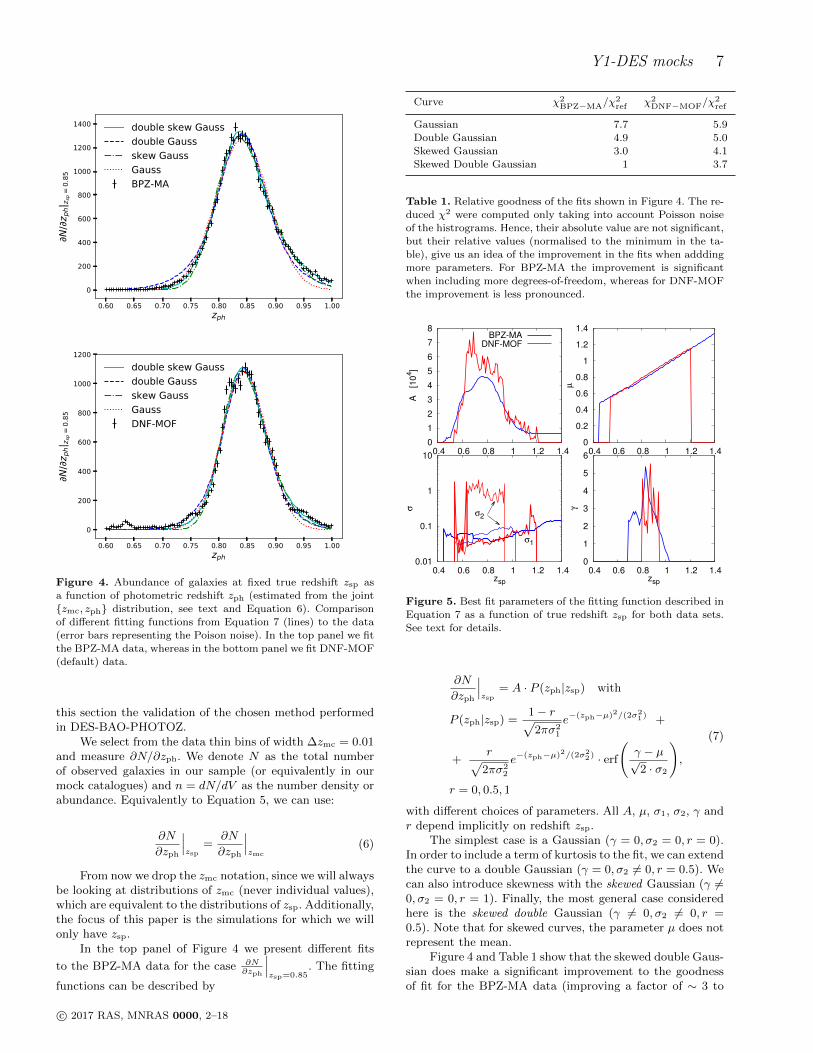
Figure 4. Abundance of galaxies at fixed true redshift zsp as

a function of photometric redshift zph (estimated from the joint

zmc, zph distribution, see text and Equation 6). Comparisonof different fitting functions from Equation 7 (lines) to the data

(error bars representing the Poison noise). In the top panel we fit

the BPZ-MA data, whereas in the bottom panel we fit DNF-MOF(default) data.

this section the validation of the chosen method performedin DES-BAO-PHOTOZ.

We select from the data thin bins of width ∆zmc = 0.01and measure ∂N/∂zph. We denote N as the total numberof observed galaxies in our sample (or equivalently in ourmock catalogues) and n = dN/dV as the number density orabundance. Equivalently to Equation 5, we can use:

∂N

∂zph

∣∣∣zsp

=∂N

∂zph

∣∣∣zmc

(6)

From now we drop the zmc notation, since we will alwaysbe looking at distributions of zmc (never individual values),which are equivalent to the distributions of zsp. Additionally,the focus of this paper is the simulations for which we willonly have zsp.

In the top panel of Figure 4 we present different fits

to the BPZ-MA data for the case ∂N∂zph

∣∣∣zsp=0.85

. The fitting

functions can be described by

Curve χ2BPZ−MA/χ

2ref χ2

DNF−MOF/χ2ref

Gaussian 7.7 5.9Double Gaussian 4.9 5.0

Skewed Gaussian 3.0 4.1

Skewed Double Gaussian 1 3.7

Table 1. Relative goodness of the fits shown in Figure 4. The re-

duced χ2 were computed only taking into account Poisson noise

of the histrograms. Hence, their absolute value are not significant,but their relative values (normalised to the minimum in the ta-

ble), give us an idea of the improvement in the fits when addding

more parameters. For BPZ-MA the improvement is significantwhen including more degrees-of-freedom, whereas for DNF-MOF

the improvement is less pronounced.

0

1

2

3

4

5

6

7

8

0.4 0.6 0.8 1 1.2 1.4

A [10

4]

BPZ-MADNF-MOF

0

0.2

0.4

0.6

0.8

1

1.2

1.4

0.4 0.6 0.8 1 1.2 1.4

µ 0

1

2

3

4

5

6

0.4 0.6 0.8 1 1.2 1.4γ

zsp

0.01

0.1

1

10

0.4 0.6 0.8 1 1.2 1.4

σ

zsp

σ1

σ2

Figure 5. Best fit parameters of the fitting function described in

Equation 7 as a function of true redshift zsp for both data sets.

See text for details.

∂N

∂zph

∣∣∣zsp

= A · P (zph|zsp) with

P (zph|zsp) =1− r√2πσ2

1

e−(zph−µ)2/(2σ21) +

+r√

2πσ22

e−(zph−µ)2/(2σ22) · erf

(γ − µ√2 · σ2

),

r = 0, 0.5, 1

(7)

with different choices of parameters. All A, µ, σ1, σ2, γ andr depend implicitly on redshift zsp.

The simplest case is a Gaussian (γ = 0, σ2 = 0, r = 0).In order to include a term of kurtosis to the fit, we can extendthe curve to a double Gaussian (γ = 0, σ2 6= 0, r = 0.5). Wecan also introduce skewness with the skewed Gaussian (γ 6=0, σ2 = 0, r = 1). Finally, the most general case consideredhere is the skewed double Gaussian (γ 6= 0, σ2 6= 0, r =0.5). Note that for skewed curves, the parameter µ does notrepresent the mean.

Figure 4 and Table 1 show that the skewed double Gaus-sian does make a significant improvement to the goodnessof fit for the BPZ-MA data (improving a factor of ∼ 3 to

c© 2017 RAS, MNRAS 0000, 2–18

8 Avila et al.

0.6 0.8 1.0 1.2 1.4zsp

0.0

2.5

5.0

7.5

10.0

12.5

15.0

17.5

n(z s

p)[1

04 (

Mpc

/h)

3 ]

Data BPZ-MAData DNF-MOFMocks BPZ-MAMocks DNF-MOF

0.60 0.65 0.70 0.75 0.80 0.85 0.90 0.95 1.00zph

0.0

2.5

5.0

7.5

10.0

12.5

15.0

17.5

20.0

n(z p

h)[1

04 (

Mpc

/h)

3 ]

Data BPZ-MAData DNF-MOFMocks BPZ-MAMocks DNF-MOF

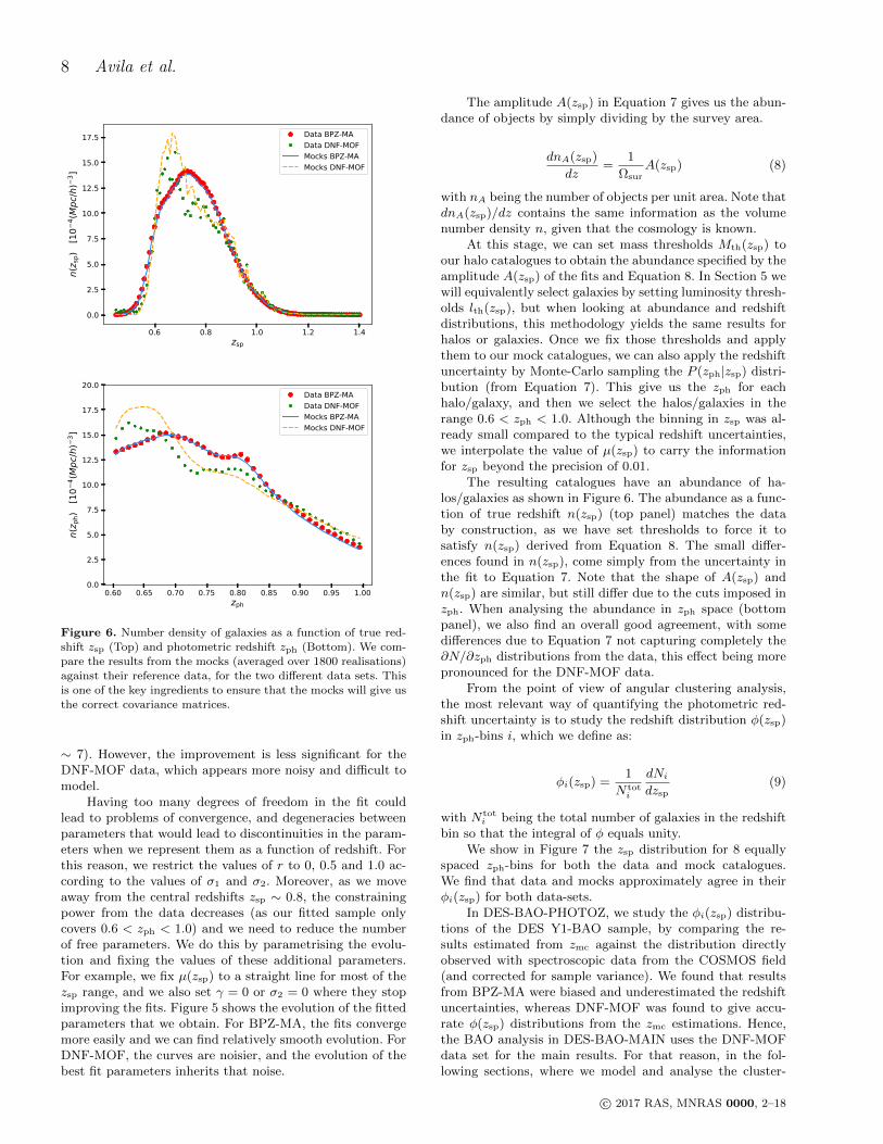
Figure 6. Number density of galaxies as a function of true red-

shift zsp (Top) and photometric redshift zph (Bottom). We com-

pare the results from the mocks (averaged over 1800 realisations)against their reference data, for the two different data sets. This

is one of the key ingredients to ensure that the mocks will give us

the correct covariance matrices.

∼ 7). However, the improvement is less significant for theDNF-MOF data, which appears more noisy and difficult tomodel.

Having too many degrees of freedom in the fit couldlead to problems of convergence, and degeneracies betweenparameters that would lead to discontinuities in the param-eters when we represent them as a function of redshift. Forthis reason, we restrict the values of r to 0, 0.5 and 1.0 ac-cording to the values of σ1 and σ2. Moreover, as we moveaway from the central redshifts zsp ∼ 0.8, the constrainingpower from the data decreases (as our fitted sample onlycovers 0.6 < zph < 1.0) and we need to reduce the numberof free parameters. We do this by parametrising the evolu-tion and fixing the values of these additional parameters.For example, we fix µ(zsp) to a straight line for most of thezsp range, and we also set γ = 0 or σ2 = 0 where they stopimproving the fits. Figure 5 shows the evolution of the fittedparameters that we obtain. For BPZ-MA, the fits convergemore easily and we can find relatively smooth evolution. ForDNF-MOF, the curves are noisier, and the evolution of thebest fit parameters inherits that noise.

The amplitude A(zsp) in Equation 7 gives us the abun-dance of objects by simply dividing by the survey area.

dnA(zsp)

dz=

1

ΩsurA(zsp) (8)

with nA being the number of objects per unit area. Note thatdnA(zsp)/dz contains the same information as the volumenumber density n, given that the cosmology is known.

At this stage, we can set mass thresholds Mth(zsp) toour halo catalogues to obtain the abundance specified by theamplitude A(zsp) of the fits and Equation 8. In Section 5 wewill equivalently select galaxies by setting luminosity thresh-olds lth(zsp), but when looking at abundance and redshiftdistributions, this methodology yields the same results forhalos or galaxies. Once we fix those thresholds and applythem to our mock catalogues, we can also apply the redshiftuncertainty by Monte-Carlo sampling the P (zph|zsp) distri-bution (from Equation 7). This give us the zph for eachhalo/galaxy, and then we select the halos/galaxies in therange 0.6 < zph < 1.0. Although the binning in zsp was al-ready small compared to the typical redshift uncertainties,we interpolate the value of µ(zsp) to carry the informationfor zsp beyond the precision of 0.01.

The resulting catalogues have an abundance of ha-los/galaxies as shown in Figure 6. The abundance as a func-tion of true redshift n(zsp) (top panel) matches the databy construction, as we have set thresholds to force it tosatisfy n(zsp) derived from Equation 8. The small differ-ences found in n(zsp), come simply from the uncertainty inthe fit to Equation 7. Note that the shape of A(zsp) andn(zsp) are similar, but still differ due to the cuts imposed inzph. When analysing the abundance in zph space (bottompanel), we also find an overall good agreement, with somedifferences due to Equation 7 not capturing completely the∂N/∂zph distributions from the data, this effect being morepronounced for the DNF-MOF data.

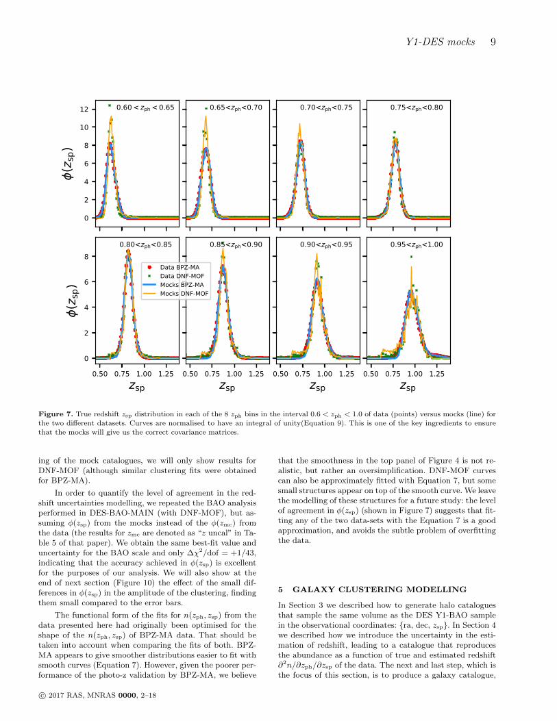
From the point of view of angular clustering analysis,the most relevant way of quantifying the photometric red-shift uncertainty is to study the redshift distribution φ(zsp)in zph-bins i, which we define as:

φi(zsp) =1

N toti

dNidzsp

(9)

with N toti being the total number of galaxies in the redshift

bin so that the integral of φ equals unity.We show in Figure 7 the zsp distribution for 8 equally

spaced zph-bins for both the data and mock catalogues.We find that data and mocks approximately agree in theirφi(zsp) for both data-sets.

In DES-BAO-PHOTOZ, we study the φi(zsp) distribu-tions of the DES Y1-BAO sample, by comparing the re-sults estimated from zmc against the distribution directlyobserved with spectroscopic data from the COSMOS field(and corrected for sample variance). We found that resultsfrom BPZ-MA were biased and underestimated the redshiftuncertainties, whereas DNF-MOF was found to give accu-rate φ(zsp) distributions from the zmc estimations. Hence,the BAO analysis in DES-BAO-MAIN uses the DNF-MOFdata set for the main results. For that reason, in the fol-lowing sections, where we model and analyse the cluster-

c© 2017 RAS, MNRAS 0000, 2–18

Y1-DES mocks 9

0

2

4

6

8

10

12

(zsp

)

0.60 < zph < 0.65 0.65<zph<0.70 0.70<zph<0.75 0.75<zph<0.80

0.50 0.75 1.00 1.25zsp

0

2

4

6

8

(zsp

)

0.80<zph<0.85

0.50 0.75 1.00 1.25zsp

0.85<zph<0.90

Data BPZ-MAData DNF-MOFMocks BPZ-MAMocks DNF-MOF

0.50 0.75 1.00 1.25zsp

0.90<zph<0.95

0.50 0.75 1.00 1.25zsp

0.95<zph<1.00

Figure 7. True redshift zsp distribution in each of the 8 zph bins in the interval 0.6 < zph < 1.0 of data (points) versus mocks (line) forthe two different datasets. Curves are normalised to have an integral of unity(Equation 9). This is one of the key ingredients to ensure

that the mocks will give us the correct covariance matrices.

ing of the mock catalogues, we will only show results forDNF-MOF (although similar clustering fits were obtainedfor BPZ-MA).

In order to quantify the level of agreement in the red-shift uncertainties modelling, we repeated the BAO analysisperformed in DES-BAO-MAIN (with DNF-MOF), but as-suming φ(zsp) from the mocks instead of the φ(zmc) fromthe data (the results for zmc are denoted as “z uncal” in Ta-ble 5 of that paper). We obtain the same best-fit value anduncertainty for the BAO scale and only ∆χ2/dof = +1/43,indicating that the accuracy achieved in φ(zsp) is excellentfor the purposes of our analysis. We will also show at theend of next section (Figure 10) the effect of the small dif-ferences in φ(zsp) in the amplitude of the clustering, findingthem small compared to the error bars.

The functional form of the fits for n(zph, zsp) from thedata presented here had originally been optimised for theshape of the n(zph, zsp) of BPZ-MA data. That should betaken into account when comparing the fits of both. BPZ-MA appears to give smoother distributions easier to fit withsmooth curves (Equation 7). However, given the poorer per-formance of the photo-z validation by BPZ-MA, we believe

that the smoothness in the top panel of Figure 4 is not re-alistic, but rather an oversimplification. DNF-MOF curvescan also be approximately fitted with Equation 7, but somesmall structures appear on top of the smooth curve. We leavethe modelling of these structures for a future study: the levelof agreement in φ(zsp) (shown in Figure 7) suggests that fit-ting any of the two data-sets with the Equation 7 is a goodapproximation, and avoids the subtle problem of overfittingthe data.

5 GALAXY CLUSTERING MODELLING

In Section 3 we described how to generate halo cataloguesthat sample the same volume as the DES Y1-BAO samplein the observational coordinates: ra, dec, zsp. In Section 4we described how we introduce the uncertainty in the esti-mation of redshift, leading to a catalogue that reproducesthe abundance as a function of true and estimated redshift∂2n/∂zph/∂zsp of the data. The next and last step, which isthe focus of this section, is to produce a galaxy catalogue,

c© 2017 RAS, MNRAS 0000, 2–18

10 Avila et al.

able to reproduce the data clustering. For this, we will in-troduce hybrid HOD-HAM modelling.

Halo Abundance Matching (HAM). So far, all theclustering measurements shown throughout this paper wereobtained from halo catalogues at a given mass threshold.But observed clustering is typically measured from galaxycatalogues with a magnitude-limited sample with the asso-ciated selection effects and, more generally, with redshift-dependent colour and magnitude cuts.

The basis of the HAM model is to assume that themost massive halo in a simulation would correspond to themost luminous galaxy in the observations and that we coulddo a one-to-one mapping in rank order. This is certainlyvery optimistic and realistic models need to add a scatterin the Luminosity-Mass relation (L−M) that will decreasethe clustering for a magnitude-limited sample (Conroy et al.2006; Behroozi et al. 2010; Trujillo-Gomez et al. 2011; Nuzaet al. 2013; Guo et al. 2016).

halogen was designed to only deal with main halos,neglecting subhalos. This limits the potential of HAM, aswe can not use its natural extension to subhalos SHAM,where there is more freedom in the modelling by treatingseparately satellite and central galaxies (see e.g. Favole et al.2015).

Nevertheless, substructure can be easily added to amain halo catalogue using a Halo Occupation Distributiontechnique.

Halo Occupation Distribution (HOD). We know thathalos can host more than one galaxy, especially massivehalos which match galaxy clusters. If we attribute a numberof galaxies Ngal that is an increasing function of the halomass (Mh) to a halo mock catalogue, the clustering will beenhanced, since massive halos will be over-represented (asoccurs in reality for a magnitude-limited sample). This isthe basis of the HOD methods (Jing et al. 1998; Peacock &Smith 2000; Berlind & Weinberg 2002; Zheng et al. 2005;Guo et al. 2012; Zehavi et al. 2011; Carretero et al. 2015;Rodrıguez-Torres et al. 2016; Skibba & Sheth 2009).

The details of the HOD and HAM need to be matchedto observations via parameter fitting. This process can beparticularly difficult if one aims at having a general modelthat serves for any sample with any magnitude and colourcut at any redshift (e.g. Carretero et al. 2015). Additionally,the HOD implementation will determine the small scale clus-tering corresponding to the correlation between galaxies ofthe same halo (Cooray & Sheth 2002). However, this is be-yond the scope of this paper and we will only aim to matchthe large scale clustering of the Y1-BAO sample.

In this paper we combine the two processes: first weadd substructure with a HOD model, and in a later stepwe select the galaxies that enter into our sample following aHAM prescription.

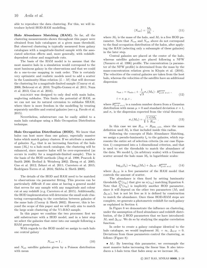
With regards to the HOD model we assign to each haloone central galaxy

Ncent = 1 , (10)

and Nsat satellite galaxies given by a Poisson distributionwith mean

〈Nsat〉 =Mh

M1, (11)

where Mh is the mass of the halo, and M1 is a free HOD pa-rameter. Note that Ncen and Nsat above do not correspondto the final occupation distribution of the halos, after apply-ing the HAM (selecting only a subsample of these galaxies)in the later step.

Central galaxies are placed at the center of the halo,whereas satellite galaxies are placed following a NFW(Navarro et al. 1996) profile. The concentration (a parame-ter of the NFW profile) is determined from the mass by themass-concentration relation given in Klypin et al. (2016).The velocities of the central galaxies are taken from the hosthalo, whereas the velocities of the satellite have an additionaldispersion:

vsat i = vhalo i +1√3σv(Mh) ·Rgauss

µ=0 σ=1 ,

i = x, y, z ,

(12)

where Rgaussµ=0 σ=1 is a random number drawn from a Gaussian

distribution with mean µ = 0 and standard deviation σ = 1,and σv is the dispersion expected from the virial theorem:

σv(Mh) =

√1

5

GMh

Rvir. (13)

In this case we use Rvir = R200, crit, since the massdefinition used Mh is that included inside this radius.

Following the concepts of Halo Abundance Matching,we assign a pseudo-luminosity lp to the galaxies, which rep-resents the entire set of selection criteria (in our case Equa-tion 1) compressed into a 1-dimendional criterion, and thatis used to set the thresholds to match the abundance ofthe data. We model lp (in arbitrary scales) with a Gaussianscatter around the halo mass Mh in logarithmic scales:

log10(lp) = log10(Mh) + ∆LM ·Rgaussµ=0 σ=1 (14)

where ∆LM is a free parameter of the HAM model thatcontrols the amount of scatter.

The abundance is then fixed by setting luminositythresholds lthp (zsp) that give us n(zsp) matching Equation 8.Note that lthp (zsp) is implicitly another HOD parameter,since it will depend on the other two parameters (M1 and∆LM ), but is not let free as it is defined by constructionto match the abundance. Once these HOD-HAM steps arecomplete, we generate a photometric redshift for each galaxyas explained in Section 4.

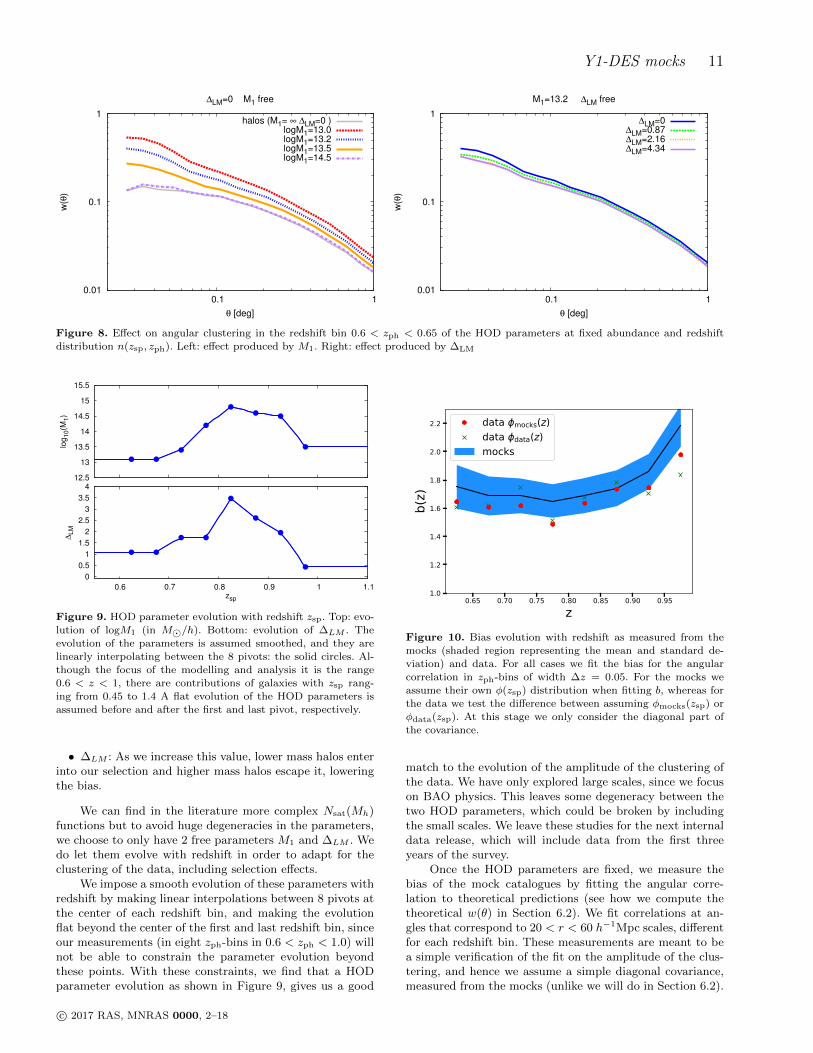
In Figure 8 we demonstrate the influence on clustering,under the assumption of fixed abundance and redshift distri-bution, of the 2 HOD parameters that we have introduced:M1 and ∆LM . We do so by studying the angular correlationfunction.

In order to create a galaxy catalogue identical to thehalo catalogue, we would implement M1 = ∞, ∆LM = 0.Deviations from those parameters control the clustering, asfollows (Figure 8):

• M1: By lowering this parameter, we oversample themost massive halos increasing the linear bias. It also intro-duces a 1-halo term that fades away as we increase M1.

c© 2017 RAS, MNRAS 0000, 2–18

Y1-DES mocks 11

0.01

0.1

1

0.1 1

w(θ

)

θ [deg]

∆LM=0 M1 free

halos (M1= ∞ ∆LM=0 )logM1=13.0logM1=13.2logM1=13.5logM1=14.5

0.01

0.1

1

0.1 1

w(θ

)

θ [deg]

M1=13.2 ∆LM free

∆LM=0∆LM=0.87∆LM=2.16∆LM=4.34

Figure 8. Effect on angular clustering in the redshift bin 0.6 < zph < 0.65 of the HOD parameters at fixed abundance and redshiftdistribution n(zsp, zph). Left: effect produced by M1. Right: effect produced by ∆LM

12.5

13

13.5

14

14.5

15

15.5

log

10(M

1)

0

0.5

1

1.5

2

2.5

3

3.5

4

0.6 0.7 0.8 0.9 1 1.1

∆LM

zsp

Figure 9. HOD parameter evolution with redshift zsp. Top: evo-lution of logM1 (in M/h). Bottom: evolution of ∆LM . The

evolution of the parameters is assumed smoothed, and they are

linearly interpolating between the 8 pivots: the solid circles. Al-though the focus of the modelling and analysis it is the range

0.6 < z < 1, there are contributions of galaxies with zsp rang-

ing from 0.45 to 1.4 A flat evolution of the HOD parameters isassumed before and after the first and last pivot, respectively.

• ∆LM : As we increase this value, lower mass halos enterinto our selection and higher mass halos escape it, loweringthe bias.

We can find in the literature more complex Nsat(Mh)functions but to avoid huge degeneracies in the parameters,we choose to only have 2 free parameters M1 and ∆LM . Wedo let them evolve with redshift in order to adapt for theclustering of the data, including selection effects.

We impose a smooth evolution of these parameters withredshift by making linear interpolations between 8 pivots atthe center of each redshift bin, and making the evolutionflat beyond the center of the first and last redshift bin, sinceour measurements (in eight zph-bins in 0.6 < zph < 1.0) willnot be able to constrain the parameter evolution beyondthese points. With these constraints, we find that a HODparameter evolution as shown in Figure 9, gives us a good

0.65 0.70 0.75 0.80 0.85 0.90 0.95z

1.0

1.2

1.4

1.6

1.8

2.0

2.2b(

z)data mocks(z)data data(z)mocks

Figure 10. Bias evolution with redshift as measured from the

mocks (shaded region representing the mean and standard de-viation) and data. For all cases we fit the bias for the angular

correlation in zph-bins of width ∆z = 0.05. For the mocks weassume their own φ(zsp) distribution when fitting b, whereas forthe data we test the difference between assuming φmocks(zsp) or

φdata(zsp). At this stage we only consider the diagonal part of

the covariance.

match to the evolution of the amplitude of the clustering ofthe data. We have only explored large scales, since we focuson BAO physics. This leaves some degeneracy between thetwo HOD parameters, which could be broken by includingthe small scales. We leave these studies for the next internaldata release, which will include data from the first threeyears of the survey.

Once the HOD parameters are fixed, we measure thebias of the mock catalogues by fitting the angular corre-lation to theoretical predictions (see how we compute thetheoretical w(θ) in Section 6.2). We fit correlations at an-gles that correspond to 20 < r < 60 h−1Mpc scales, differentfor each redshift bin. These measurements are meant to bea simple verification of the fit on the amplitude of the clus-tering, and hence we assume a simple diagonal covariance,measured from the mocks (unlike we will do in Section 6.2).

c© 2017 RAS, MNRAS 0000, 2–18

12 Avila et al.

In Figure 10 we show the bias evolution recovered from themock catalogues, with the blue band representing the 1-σ re-gion computed as the standard deviation of best fit of eachmock.

We also present in Figure 10 the bias measured fromthe data. In red we show the measured bias if we assume thesame redshift distribution φi(zsp) as in the mocks, whereasin green we show the measured bias assuming the φi(zsp)estimated from the data itself. The main conclusion of thisplot is that the amplitude of the clustering of the data (redcircles) agrees within 1-σ with the mocks. We notice a trendof the mocks having a slightly higher amplitude than thedata, this effect is small compared to the uncertainties, butwill be studied in more detail for future releases. This plotalso shows us that the small differences between φmocks andφdata in Figure 7 do not have a significant effect in the clus-tering, since all shifts are smaller than the σ (and most ofthem being much smaller).

Looking at the mean halo mass of the catalogues we findthat our Y1-BAO sample probes halo masses between 1.3×1013M/h and 2.1 × 1013M/h depending on the redshiftrange.

6 CLUSTERING RESULTS

In previous sections we designed a method to reproduce allthe relevant properties of the Y1-BAO sample for cluster-ing analysis. In this section we fix all the modelling andparameters and run Nmocks = 1800 realisations with differ-ent initial conditions. We analyse the clustering of all thosemocks using different estimators in different spaces (wi(θ),ξ(r), Cl)), and their covariance matrices. We also comparethose statistics with theoretical models, and measurementsfrom the data.

6.1 Theoretical modelling

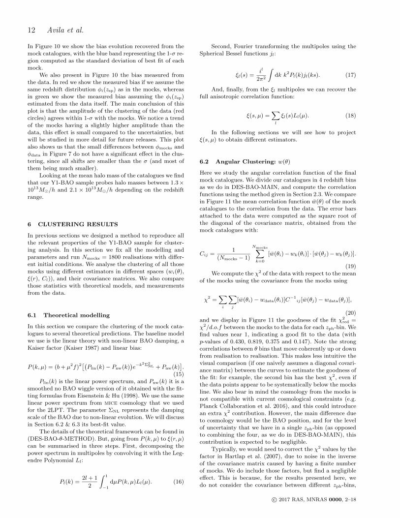
In this section we compare the clustering of the mock cata-logues to several theoretical predictions. The baseline modelwe use is the linear theory with non-linear BAO damping, aKaiser factor (Kaiser 1987) and linear bias:

P (k, µ) = (b+ µ2f)2[(Plin(k)− Pnw(k))e−k

2Σ2NL + Pnw(k)

].

(15)Plin(k) is the linear power spectrum, and Pnw(k) it is a

smoothed no BAO wiggle version of it obtained with the fit-ting formulas from Eisenstein & Hu (1998). We use the samelinear power spectrum from mice cosmology that we usedfor the 2LPT. The parameter ΣNL represents the dampingscale of the BAO due to non-linear evolution. We will discussin Section 6.2 & 6.3 its best-fit value.

The details of the theoretical framework can be found in(DES-BAO-θ-METHOD). But, going from P (k, µ) to ξ(r, µ)can be summarised in three steps. First, decomposing thepower spectrum in multipoles by convolving it with the Leg-endre Polynomial Ll:

Pl(k) =2l + 1

2

∫ 1

−1

dµP (k, µ)Ll(µ). (16)

Second, Fourier transforming the multipoles using theSpherical Bessel functions jl:

ξl(s) =il

2π2

∫dk k2Pl(k)jl(ks). (17)

And, finally, from the ξl multipoles we can recover thefull anisotropic correlation function:

ξ(s, µ) =∑l

ξl(s)Ll(µ). (18)

In the following sections we will see how to projectξ(s, µ) to obtain different estimators.

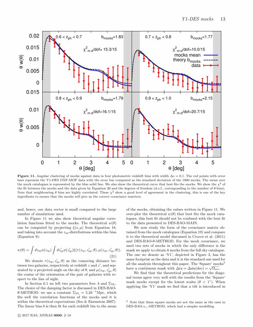
6.2 Angular Clustering: w(θ)

Here we study the angular correlation function of the finalmock catalogues. We divide our catalogues in 4 redshift binsas we do in DES-BAO-MAIN, and compute the correlationfunctions using the method given in Section 2.3. We comparein Figure 11 the mean correlation function w(θ) of the mockcatalogues to the correlation from the data. The error barsattached to the data were computed as the square root ofthe diagonal of the covariance matrix, obtained from themock catalogues with:

Cij =1

(Nmocks − 1)

Nmocks∑k=0

[w(θi)−wk(θi)] · [w(θj)−wk(θj)].

(19)We compute the χ2 of the data with respect to the mean

of the mocks using the covariance from the mocks using

χ2 =∑i

∑j

[w(θi)− wdata(θi)]C−1

ij [w(θj)− wdata(θj)],

(20)and we display in Figure 11 the goodness of the fit χ2

red =χ2/d.o.f between the mocks to the data for each zph-bin. Wefind values near 1, indicating a good fit to the data (withp-values of 0.430, 0.819, 0.375 and 0.147). Note the strongcorrelations between θ bins that move coherently up or downfrom realisation to realisation. This makes less intuitive thevisual comparison (if one naively assumes a diagonal covari-ance matrix) between the curves to estimate the goodness ofthe fit: for example, the second bin has the best χ2, even ifthe data points appear to be systematically below the mocksline. We also bear in mind the cosmology from the mocks isnot compatible with current cosmological constraints (e.g.Planck Collaboration et al. 2016), and this could introducean extra χ2 contribution. However, the main difference dueto cosmology would be the BAO position, and for the levelof uncertainty that we have in a single zph-bin (as opposedto combining the four, as we do in DES-BAO-MAIN), thiscontribution is expected to be negligible.

Typically, we would need to correct the χ2 values by thefactor in Hartlap et al. (2007), due to noise in the inverseof the covariance matrix caused by having a finite numberof mocks. We do include those factors, but find a negligibleeffect. This is because, for the results presented here, wedo not consider the covariance between different zph-bins,

c© 2017 RAS, MNRAS 0000, 2–18

Y1-DES mocks 13

0

0.005

0.01

0.015

0.02

θ w

(θ)

0.6 < zph < 0.7

χ2m-d/dof= 15.3/15

bmocks=1.83 0.7 < zph < 0.8

χ2m-d/dof=10.0/15

bmocks=1.77

mocks meantheory bmocks

data

0

0.005

0.01

0.015

0 1 2 3 4 5

θ w

(θ)

θ [deg]

0.8 < zph < 0.9

χ2m-d/dof=16.1/15

bmocks=1.79

0 1 2 3 4 5θ [deg]

0.9 < zph < 1.0

χ2m-d/dof=20.7/15

bmocks=2.15

Figure 11. Angular clustering of mocks against data in four photometric redshift bins with width ∆z = 0.1. The red points with errorbars represent the Y1-DES DNF-MOF data with the error bar computed as the standard deviation of the 1800 mocks. The mean over

the mock catalogues is represented by the blue solid line. We also show the theoretical curve that best fits the mocks. We show the χ2 of

the fit between the mocks and the data given by Equation 20 and the degrees of freedom (d.o.f., corresponding to the number of θ-bins).Note that neighbouring θ bins are highly correlated. These χ2 show a good level of agreement in the clustering, this is one of the key

ingredients to ensure that the mocks will give us the correct covariance matrices.

and, hence, our data vector is small compared to the largenumber of simulations used.

In Figure 11 we also show theoretical angular corre-lation functions fitted to the mocks. The theoretical w(θ)can be computed by projecting ξ(s, µ) from Equation 18,and taking into account the zsp-distributions within the bins(Equation 9):

w(θ) =

∫dzspφ(zsp)

∫dz′spφ(z′sp)ξ(r(zsp, z

′sp, θ), µ(zsp, z

′sp, θ)).

(21)We denote r(zsp, z

′sp, θ) as the comoving distance be-

tween two galaxies, respectively at redshift z and z′, and sep-arated by a projected angle on the sky of θ, and µ(zsp, z

′sp, θ)

the cosine of the orientation of the pair of galaxies with re-spect to the line of sight.

In Section 6.1 we left two parameters free: b and ΣNL.The choice of the damping factor is discussed in DES-BAO-θ-METHOD: we use a constant ΣNL = 5.2h−1Mpc, whichfits well the correlation functions of the mocks and it iswithin the theoretical expectations (Seo & Eisenstein 2007).The linear bias b is then fit for each redshift bin to the mean

of the mocks, obtaining the values written in Figure 11. Weover-plot the theoretical w(θ) that best fits the mock cata-logues, this best fit should not be confused with the best fitto the data presented in DES-BAO-MAIN.

We now study the form of the covariance matrix ob-tained from the mock catalogues (Equation 19) and compareit to the theoretical model discussed in Crocce et al. (2011)and DES-BAO-θ-METHOD. For the mock covariance, weused two sets of mocks in which the only difference is themask we apply to obtain 8 mocks from the full sky catalogue.The one we denote as ‘Y1’, depicted in Figure 3, has thesame footprint as the data and it is the standard one used forall the analysis throughout this paper. The ‘Square’ mocks5

have a continuous mask with ∆ra = ∆sin(dec) =√

Ωsur.We find that the theoretical predictions for the diago-

nal terms agree very well with the results from the ‘Square’mask mocks except for the lowest scales (θ < 1). Whenapplying the ‘Y1’ mask we find that a tilt is introduced in

5 Note that these square mocks are not the same as the ones in

DES-BAO-s⊥-METHOD, which had a simpler modelling

c© 2017 RAS, MNRAS 0000, 2–18

14 Avila et al.

0 1 2 3 4 5 6-0.2

-0.1

0.0

0.1

0.2

0.3

0.4

Θ @degD

HΣM

ock

sΣ

Theo

ryL-

1

LSS BAO Sample

Square Mask0.6 < z < 0.7

0.7 < z < 0.8

0.8 < z < 0.9

0.9 < z < 1.0

0 1 2 3 4 5 6-0.2

-0.1

0.0

0.1

0.2

0.3

0.4

Θ @degD

HΣM

ock

sΣ

Theo

ryL-

1

LSS BAO Sample

Y1 Mask0.6 < z < 0.7

0.7 < z < 0.8

0.8 < z < 0.9

0.9 < z < 1.0

ææææ

æææ

ææææææææ

æææ

æ

æ

æ

ææ

æ

æ

æ

æ

æ

æ

æ

æ

æ

æ

æ

ææ

æææ

ææææ

æææææææææææææ

ææææææææææææææææææææææ

æææ

ææææææææææ

ææææææææææææææææææææææææææ

æææ

ææææææææææ

ææææææææææææææææææææææææææ

ææææ

ææææææææææ

æ

æ

æ

æ

æ

æ

æ

æ

æ

æ

æ

æ

æ

æ

æ

æ

æ

æ

ææ

æææ

ææ

æææææ

æææææææ

ææææææææ

æææææææææ

ææææææææææ

æææ

æææææææææ

æææææææææ

æææææææææææææææææææ

æææ

ææææææææ

ææææææ

ææææææææææææææ

æææææ

ææ

0 50 100 150

0

2

4

6

8

10

Θ @degD

Cov

@Θ,Θ¢ D

Θ¢ = 3.5 deg

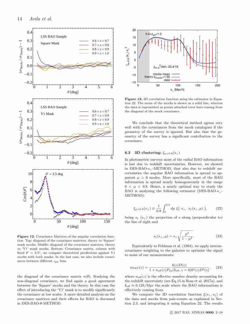
Figure 12. Covariance Matrices of the angular correlation func-tion. Top: diagonal of the covariance matrices, theory vs ‘Square’

mask mocks. Middle: diagonal of the covariance matrices, theory

vs ‘Y1’ mask mocks. Bottom: Covariance matrix, column withfixed θ′ = 3.5, we compare theoretical predictions against Y1

mocks with both masks. In the last case, we also include covari-

ances between different zph bins.

the diagonal of the covariance matrix σ(θ). Studying thenon-diagonal covariance, we find again a good agreementbetween the ‘Square’ mocks and the theory. In this case theeffect of introducing the ‘Y1’ mask is to modify significantlythe covariance at low scales. A more detailed analysis on thecovariance matrices and their effects for BAO is discussedin DES-BAO-θ-METHOD.

-15

-10

-5

0

5

10

15

20

0 50 100 150 200

ξ µ<

0.8

(s

⊥)

s⊥

2

s⊥ [Mpc/h]

0.6<zph<1.0

χm-d2/dof= 20.4/16

mocks meantheory bmocks=1.92

data

Figure 13. 3D correlation function using the estimator in Equa-

tion 22. The mean of the mocks is shown as a solid line, whereas

the data is represented as points attached error bars coming fromthe diagonal of the mock covariance.

We conclude that the theoretical method agrees verywell with the covariances from the mock catalogues if thegeometry of the survey is ignored. But also that the ge-ometry of the survey has a significant contribution to thecovariance.

6.3 3D clustering: ξµ<0.8(s⊥)

In photometric surveys most of the radial BAO informationis lost due to redshift uncertainties. However, we showedin DES-BAO-s⊥-METHOD, that also due to redshift un-certainties the angular BAO information is spread to ap-parent µ > 0 modes. More specifically, most of the BAOinformation is spread nearly homogeneously in the range0 < µ < 0.8. Hence, a nearly optimal way to study theBAO is analysing the following estimator (DES-BAO-s⊥-METHOD):

ξµ<0.8(s⊥) ≡ 1

0.8

∫ 0.8

0

dµ ξ(s⊥, s‖(s⊥, µ)

), (22)

being s‖ (s⊥) the projection of s along (perpendicular to)the line of sight and

s‖(s⊥, µ) = s⊥

õ2

1− µ2. (23)

Equivalently to Feldman et al. (1994), we apply inverse-covariance weighting to the galaxies to optimise the signalto noise of our measurements:

wFKP(z) =b(z)D(z)

1 + neff(z)Plin(keff , z = 0)b2(z)D2(z), (24)

where neff(z) is the effective number density accounting forthe redshift uncertainty (see Eq.15 in Ross et al. 2017a), andkeff ≈ 0.12h/Mpc the scale where the BAO informations iseffectively coming from.

We compute the 3D correlation function ξ(s⊥, s‖) ofthe data and mocks from pair-counts as explained in Sec-tion 2.3, and integrating it using Equation 22. The results

c© 2017 RAS, MNRAS 0000, 2–18

Y1-DES mocks 15

are shown in Figure 13, finding again a good agreement be-tween mocks and data (with a p-value of 0.20). Again, theerror-bars attached to the data come from the diagonal ofthe covariance from the mocks, and the χ2 were computedwith the covariance from the mocks.

From the theoretical point of view, we can projectξ(s, µ) from Equation 18 using Equation 22. For this we usea Gaussian uncertainty approximation, following the pro-cedure in DES-BAO-s⊥-METHOD. In this case we re-fitΣNL, expecting this to capture part of the effect of the non-gaussian tails of the redshift uncertainties. We find a bestfit value of ΣNL = 8Mpc/h. We compute the bias of themocks bmocks as the weighted average of the values obtainedin the previous subsection (Section 6.2). We plot the the-oretical prediction for this bias, finding a good agreementthat confirms the consistency of the mocks and theoreticalframework we are working on.

6.4 Clustering in Angular Harmonic space: Cl

In spectroscopic surveys, it has been shown that even thoughtheoretically ξ(r) and P (k) carry the same information indifferent spaces, in reality, when dealing with finite volume,they can be provide complementary information (Ata et al.2017). In photometric surveys one usually deals with pro-jected quantities. In this case, the complementary observ-ables are the angular correlation w(θ) and its equivalent inharmonic space, the angular power spectrum C`.

The galaxy number density contrast in a given redshiftbin δgal,i(n) can be decomposed into spherical harmonicsY`m as

δgal,i(n) =

∞∑`=0

∑m=−`

a`m,iY`m(n) , (25)

where a`m are the harmonic coefficients. The angular powerspectrum C`,i is then defined via

〈a`m,ia∗`′m′,i〉 ≡ δ``′δmm′C`,i . (26)

For data collected over the whole sky, an unbiased esti-mator of the angular power spectrum is simply the averageof the a`m coefficients over all m values:

C` =1

2`+ 1

m=∑m=−`

|a`m|2 . (27)

When performing full-sky estimations, we compute thecoefficients a`m from the pixelized density contrast mapsusing the anafast routine within HEALPiX.

In the case of partial sky coverage, the pseudo-C`method (Hivon et al. 2002) is used to measure the C`s. Themeasurement is performed with a binning of ∆` = 20 usinga resolution of Nside = 1024. A more detailed description ofthe methodology is found in DES-BAO-`-METHOD.

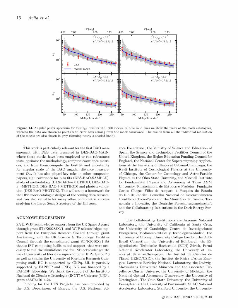
Following the procedure of previous subsections, wecompute the average and the covariance matrix for the angu-lar power spectra in each redshift bin using the 1800 mocks.The measurement is also performed on Y1 data, with errorbars estimated from the covariance matrix. The results inFigure 14 show that the angular power spectrum measuredfrom the mocks are consistent with the measurements fromdata. For simplicity, we do not include the theoretical pre-diction here, but refer to DES-BAO-`-METHOD, where we

confirm that the bias values measured in Section 6.2 fit wellthe C` from the mocks.

7 SUMMARY AND CONCLUSIONS

In this paper we have designed and analysed a set of 1800mock catalogues able to reproduce statistically the proper-ties of the Dark Energy Survey Year-1 BAO sample.

The three main properties reproduced are:

• Sampled observational volume: ra, dec, zph (Fig-ure 3).• Abundance of galaxies, redshift distribution and red-

shift uncertainty: n(zph, zsp) (Figs. 6, 7).• Clustering as a function of redshift: b(zph), wi(θ),

ξµ<0.8(s⊥) and Cil (Figs. 10, 11, 13, 14).

Matching the properties listed above guarantees thatour mock catalogues can correctly reproduce the clusteringcovariance of the data.

For the first time, we have presented a set of mock cata-logues capable to reproduce simultaneously the clustering ofa photometric sample together with an accurate descriptionof redshift distribution and uncertainties.

Throughout the paper we described in detail the waywe design the galaxy catalogues, dividing the sections bythe different physical modelling involved, following the threebullet points above. However, some of the steps involvedwere somehow coupled to previous or later sections.

Once all the parameters and models have been fixed,catalogues are created following sequentially these steps:

• Generate halo catalogues with halogen at fixed red-shifts in cubic volumes. (Section 3.1)• Compose a full sky lightcone by superposing snapshots

in redshift shells and using periodic conditions. (Section 3.2)• Add 1 central galaxy and Nsat satellite galaxies to each

halo using Equation 11. (Section 5)• Assign a luminosity lp to each galaxy, based on the halo

mass, using Equation 14. Then, select only the galaxies withlp > lth(zsp) (Section 5).• Draw a photometric redshift zph for each galaxy from

the distribution P (zph|zsp) in Equation 7. Then, select onlygalaxies in the range of interest 0.6 < zph < 1 (Section 4).• Apply the survey mask. (Section 3.3)

Some of the steps listed above involved parameters thathad to be adjusted to the data or to other simulations beforestarting producing the final batch of mock catalogues. Themain fitted ingredients of the modelling are:

• halogen parameters (α(Mh),fvel(Mh)) were tuned toreproduce the halo clustering and velocity distributions ofthe reference N -Body simulation mice as a function of massand redshift. The input Halo Mass Function was also par-tially tuned to the simulation.• We modelled n(zph, zsp) by fitting a double skewed

Gaussian to ∂n∂zph

∣∣∣zsp

(Equation 7) from the data for all zsp.

• We explored the HOD parameter spaceM1(zsp),∆LM (zsp) to reproduce the bias evolutionb(zsp) from the data. Simultaneously, the luminosity thresh-olds lth(zsp) need to be readjusted for each run in order to

match the amplitude of ∂n∂zph

∣∣∣zsp

.

c© 2017 RAS, MNRAS 0000, 2–18

16 Avila et al.

10-5

10-4

C`

0.6<zph<0.7

χ2 /dof =12.7/12

datamocks mean

0.7<zph<0.8

χ2 /dof =19.0/12

50 100 150 200 250Multipole mode `

10-5

10-4

C`

0.8<zph<0.9

χ2 /dof =12.6/12

50 100 150 200 250Multipole mode `

0.9<zph<1.0

χ2 /dof =17.3/12

0.751.002.004.00θ [deg]

0.751.002.004.00θ [deg]

Figure 14. Angular power spectrum for four zph bins for the 1800 mocks. In blue solid lines we show the mean of the mock catalogues,

whereas the data are shown as points with error bars coming from the mock covariance. The results from all the individual realisation

of the mocks are also shown in grey (forming nearly a shaded band).

This work is particularly relevant for the first BAO mea-surement with DES data presented in DES-BAO-MAIN,where these mocks have been employed to run robustnesstests, optimise the methodology, compute covariance matri-ces, and from them compute the best fit and uncertaintyfor angular scale of the BAO angular distance measure-ment DA. It has also played key roles in other companionpapers, e.g.: covariance for bias fits (DES-BAO-SAMPLE),study of methodology (DES-BAO-θ-METHOD, DES-BAO-s⊥-METHOD, DES-BAO-`-METHOD) and photo-z valida-tion (DES-BAO-PHOTOZ). This will set up a framework forthe DES mock catalogue designs of the coming data releases,and can also valuable for many other photometric surveysstudying the Large Scale Structure of the Universe.

ACKNOWLEDGEMENTS

SA & WJP acknowledge support from the UK Space Agencythrough grant ST/K00283X/1, and WJP acknowledges sup-port from the European Research Council through grantDarksurvey, and the UK Science & Technology FacilitiesCouncil through the consolidated grant ST/K0090X/1 SAthanks IFT computing facilities and support, that were nec-essary to run the simulations and fits. NB acknowledges theuse of University of Florida’s supercomputer HiPerGator 2.0as well as thanks the University of Florida’s Research Com-puting staff. HC is supported by CNPq. ML is partiallysupported by FAPESP and CNPq. NK was financed by aFAPESP fellowship. We thank the support of the InstitutoNacional de Ciencia e Tecnologia (INCT) e-Universe (CNPqgrant 465376/2014-2).

Funding for the DES Projects has been provided bythe U.S. Department of Energy, the U.S. National Sci-

ence Foundation, the Ministry of Science and Education ofSpain, the Science and Technology Facilities Council of theUnited Kingdom, the Higher Education Funding Council forEngland, the National Center for Supercomputing Applica-tions at the University of Illinois at Urbana-Champaign, theKavli Institute of Cosmological Physics at the Universityof Chicago, the Center for Cosmology and Astro-ParticlePhysics at the Ohio State University, the Mitchell Institutefor Fundamental Physics and Astronomy at Texas A&MUniversity, Financiadora de Estudos e Projetos, FundacaoCarlos Chagas Filho de Amparo a Pesquisa do Estadodo Rio de Janeiro, Conselho Nacional de DesenvolvimentoCientıfico e Tecnologico and the Ministerio da Ciencia, Tec-nologia e Inovacao, the Deutsche Forschungsgemeinschaftand the Collaborating Institutions in the Dark Energy Sur-vey.

The Collaborating Institutions are Argonne NationalLaboratory, the University of California at Santa Cruz,the University of Cambridge, Centro de InvestigacionesEnergeticas, Medioambientales y Tecnologicas-Madrid, theUniversity of Chicago, University College London, the DES-Brazil Consortium, the University of Edinburgh, the Ei-dgenossische Technische Hochschule (ETH) Zurich, FermiNational Accelerator Laboratory, the University of Illi-nois at Urbana-Champaign, the Institut de Ciencies del’Espai (IEEC/CSIC), the Institut de Fısica d’Altes Ener-gies, Lawrence Berkeley National Laboratory, the Ludwig-Maximilians Universitat Munchen and the associated Ex-cellence Cluster Universe, the University of Michigan, theNational Optical Astronomy Observatory, the University ofNottingham, The Ohio State University, the University ofPennsylvania, the University of Portsmouth, SLAC NationalAccelerator Laboratory, Stanford University, the University

c© 2017 RAS, MNRAS 0000, 2–18

Y1-DES mocks 17

of Sussex, Texas A&M University, and the OzDES Member-ship Consortium.

Based in part on observations at Cerro Tololo Inter-American Observatory, National Optical Astronomy Obser-vatory, which is operated by the Association of Universitiesfor Research in Astronomy (AURA) under a cooperativeagreement with the National Science Foundation.

The DES data management system is supported bythe National Science Foundation under Grant NumbersAST-1138766 and AST-1536171. The DES participants fromSpanish institutions are partially supported by MINECOunder grants AYA2015-71825, ESP2015-66861, FPA2015-68048, SEV-2016-0588, SEV-2016-0597, and MDM-2015-0509, some of which include ERDF funds from the EuropeanUnion. IFAE is partially funded by the CERCA programof the Generalitat de Catalunya. Research leading to theseresults has received funding from the European ResearchCouncil under the European Union’s Seventh FrameworkProgram (FP7/2007-2013) including ERC grant agreements240672, 291329, and 306478. We acknowledge support fromthe Australian Research Council Centre of Excellence forAll-sky Astrophysics (CAASTRO), through project numberCE110001020.

This manuscript has been authored by Fermi ResearchAlliance, LLC under Contract No. DE-AC02-07CH11359with the U.S. Department of Energy, Office of Science, Of-fice of High Energy Physics. The United States Governmentretains and the publisher, by accepting the article for pub-lication, acknowledges that the United States Governmentretains a non-exclusive, paid-up, irrevocable, world-wide li-cense to publish or reproduce the published form of thismanuscript, or allow others to do so, for United States Gov-ernment purposes.

REFERENCES

DES Collaboration: Alarcon A., Allam S., Annis J., AvilaS., Banerji M, Banik N, Bechtol N, G. M. Bernstein, E.Bertin, D. Brooks, E. Buckley-Geer, D. L. Burke, H. Ca-macho, A. Carnero Rosell, et al. 2017, submitted to MN-RAS

Alonso D., 2012, ArXiv:1210.1833Ata M., Baumgarten F., Bautista J., Beutler F., BizyaevD., Blanton M. R., Blazek J. A., Bolton A. S., BrinkmannJ., Brownstein J. R., Burtin E., Chuang C.-H., Com-parat J., Dawson K. S., de la Macorra A., et al. 2017,ArXiv:1705.06373

Avila S., Murray S. G., Knebe A., Power C., RobothamA. S. G., Garcia-Bellido J., 2015, MNRAS, 450, 1856

Behroozi P. S., Conroy C., Wechsler R. H., 2010, ApJ, 717,379

Benıtez N., 2000, ApJ, 536, 571Benıtez N., Ford H., Bouwens R., Menanteau F., BlakesleeJ., Gronwall C., Illingworth G., Meurer G., BroadhurstT. J., Clampin M., Franx M., Hartig G. F., Magee D.,Sirianni M., Ardila D. R., et al. 2004, ApJS, 150, 1

Berlind A. A., Weinberg D. H., 2002, ApJ, 575, 587Beutler F., Blake C., Colless M., Jones D. H., Staveley-Smith L., Campbell L., Parker Q., Saunders W., WatsonF., 2011, MNRAS, 416, 3017

Blake C., Kazin E. A., Beutler F., Davis T. M., Parkin-son D., Brough S., Colless M. ., Contreras C., CouchW., Croom S., Croton D., Drinkwater M. J., Forster K.,Gilbank D., Gladders M., Glazebrook et al., 2011, MN-RAS, 418, 1707

Bond J. R., Cole S., Efstathiou G., Kaiser N., 1991, ApJ,379, 440

Bond J. R., Myers S. T., 1996, ApJS, 103, 1Bouchet F. R., Colombi S., Hivon E., Juszkiewicz R., 1995,A&A, 296, 575

Camacho H., et al. , in preparationCarretero J., Castander F. J., Gaztanaga E., Crocce M.,Fosalba P., 2015, MNRAS, 447, 646

Chan K. C., et al., in preparationChuang C.-H., Kitaura F.-S., Prada F., Zhao C., Yepes G.,2015, MNRAS, 446, 2621

Chuang C.-H., Zhao C., Prada F., Munari E., Avila S.,Izard A., Kitaura F.-S., Manera M., Monaco P., MurrayS., Knebe A., Scoccola C. G., Yepes G., Garcia-Bellido J.,Marın F. A. et al., 2015, MNRAS, 452, 686

Cole S., Percival W. J., Peacock J. A., Norberg P., BaughC. M., Frenk C. S., Baldry I., Bland-Hawthorn J., BridgesT., Cannon R., Colless M., Collins C., Couch W., CrossN. J. G., Dalton G., Eke et al., 2005, MNRAS, 362, 505

Conroy C., Wechsler R. H., Kravtsov A. V., 2006, ApJ,647, 201

Cooray A., Sheth R., 2002, Phys. Rep., 372, 1Crocce M., et al. 2017, submitted to MNRASCrocce M., Cabre A., Gaztanaga E., 2011, MNRAS, 414,329

Crocce M., Castander F. J., Gaztanaga E., Fosalba P., Car-retero J., 2015, MNRAS, 453, 1513

De Vicente J., Sanchez E., Sevilla-Noarbe I., 2016, MN-RAS, 459, 3078

Diehl H. T., Abbott T. M. C., Annis J., Armstrong R.,Baruah L., Bermeo A., Bernstein G., Beynon E., BrudererC., Buckley-Geer E. J., Campbell H., Capozzi D., CarterM., Casas R., Clerkin L., et al. 2014, Proc. SPIE 9149,91490V

Dodelson S., Schneider M. D., 2013, Phys. Rev. D, 88,063537

Drlica-Wagner A., Sevilla-Noarbe I., Rykoff E. S., GruendlR. A., Yanny B., Tucker D. L., Hoyle B., Carnero RosellA., Bernstein G. M., Bechtol K., Becker M. R., Benoit-Levy A., Bertin et al., 2017, ArXiv:1708.01531

Eisenstein D. J., Hu W., 1998, ApJ, 496, 605Eisenstein D. J., Zehavi I., Hogg D. W., Scoccimarro R.,Blanton M. R., Nichol R. C., Scranton R., Seo H.-J.,Tegmark M., Zheng Z., Anderson S. F., Annis J., Bah-call N., Brinkmann J., Burles et al., 2005, ApJ, 633, 560

Favole G., Comparat J., Prada F., Yepes G., Jullo E.,Niemiec A., Kneib J.-P., Rodrıguez-Torres S. A., KlypinA., Skibba R. A., McBride C. K., Eisenstein D. J., SchlegelD. J., Nuza S. E., Chuang C.-H., Delubac, T. and Yeche,C. and Schneider, D. P. 2015, MNRAS, 461, 3421

Feldman H. A., Kaiser N., Peacock J. A., 1994, ApJ, 426,23

Fosalba P., Crocce M., Gaztanaga E., Castander F. J.,2015, MNRAS, 448, 2987

Fosalba P., Gaztanaga E., Castander F. J., Crocce M.,2015, MNRAS, 447, 1319

Fosalba P., Gaztanaga E., Castander F. J., Manera M.,

c© 2017 RAS, MNRAS 0000, 2–18

18 Avila et al.

2008, MNRAS, 391, 435Friedrich O., Eifler T., 2018, MNRAS, 473, 4150Gaztanaga E., et al. , in preparationGorski K. M., Hivon E., Banday A. J., Wandelt B. D.,Hansen F. K., Reinecke M., Bartelmann M., 2005, ApJ,622, 759

Guo H., Zehavi I., Zheng Z., 2012, ApJ, 756, 127Guo H., Zheng Z., Behroozi P. S., Zehavi I., Chuang C.-H.,Comparat J., Favole G., Gottloeber S., Klypin A., PradaF., Rodrıguez-Torres S. A., Weinberg D. H., Yepes G.,2016, MNRAS

Hartlap J., Simon P., Schneider P., 2007, A&A, 464, 399Hinshaw G., Nolta M. R., Bennett C. L., Bean R., Dore O.,Greason M. R., Halpern M., Hill R. S., Jarosik N., KogutA., Komatsu E., Limon M., Odegard N., Meyer S. S., PageL., Peiris H. V., Spergel D. N., Tucker et al., 2007, ApJS,170, 288

Hivon E., Gorski K. M., Netterfield C. B., Crill B. P.,Prunet S., Hansen F., 2002, Astrophys. J., 567, 2

Hoyle B., Gruen D., Bernstein G. M., Rau M. M., De Vi-cente J., Hartley W. G., Gaztanaga E., DeRose J., TroxelM. A., Davis C., Alarcon A., MacCrann N., Prat J.,Sanchez C., Sheldon E., et al. 2017, ArXiv: 1708.01532

Jing Y. P., Mo H. J., Borner G., 1998, ApJ, 494, 1Kaiser N., 1984, ApJ, 284, L9Kaiser N., 1987, MNRAS, 227, 1Kitaura F.-S., Rodrıguez-Torres S., Chuang C.-H., ZhaoC., Prada F., Gil-Marın H., Guo H., Yepes G., Klypin A.,Scoccola C. G., Tinker J. et al., 2016, MNRAS, 456, 4156

Klypin A., Yepes G., Gottlober S., Prada F., Heß S., 2016,MNRAS, 457, 4340

Landy S. D., Szalay A. S., 1993, ApJ, 412, 64Manera M., Scoccimarro R., Percival W. J. et al.,Samushia, L., McBride C. K., Ross A. J., Sheth R. K.,White M., Reid B. A., Sanchez, A. G., de Putter R., XuX., Berlind A. A., Brinkmann J., Maraston C., et al., 2013,MNRAS, 428, 1036

Monaco P., 2016, Galaxies, 4, 53Monaco P., Sefusatti E., Borgani S., Crocce M., Fosalba P.,Sheth R. K., Theuns T., 2013, MNRAS, 433, 2389

Moutarde F., Alimi J.-M., Bouchet F. R., Pellat R., Ra-mani A., 1991, ApJ, 382, 377

Murray S. G., Power C., Robotham A. S. G., 2013, Astron-omy and Computing, 3, 23

Navarro J. F., Frenk C. S., White S. D. M., 1996, ApJ, 462,563

Nuza S. E., Sanchez A. G., Prada F., Klypin A., SchlegelD. J., Gottlober S., Montero-Dorta A. D., Manera M.,McBride C. K., Ross A. J., Angulo R., Blanton M., BoltonA., Favole G., Samushia 2013, MNRAS, 432, 743

Peacock J. A., Smith R. E., 2000, MNRAS, 318, 1144Peebles P. J. E., Yu J. T., 1970, ApJ, 162, 815Planck Collaboration Ade P. A. R., Aghanim N., ArnaudM., Ashdown M., Aumont J., Baccigalupi C., BandayA. J., Barreiro R. B., Bartlett J. G., et al. 2016, A&A,594, A13

Pope A. C., Szapudi I., 2008, MNRAS, 389, 766Press W. H., Schechter P., 1974, ApJ, 187, 425Rodrıguez-Torres S. A., Chuang C.-H., Prada F., Guo H.,Klypin A., Behroozi P., Hahn C. H., Comparat J., YepesG., Montero-Dorta A. D., Brownstein J. R., Maraston C.,McBride C. K. et al., 2016, MNRAS, 460,1173

Ross A. J., Banik N., Avila S., Percival W. J., Dodelson S.,Garcia-Bellido J., Crocce M., Elvin-Poole J., Giannanto-nio T., Sevilla-Noarbe I., 2017, MNRAS, 472, 4456

Ross A. J., Beutler F., Chuang C.-H., Pellejero-IbanezM., Seo H.-J., Vargas-Magana M., Cuesta A. J., Perci-val W. J., Burden A., Sanchez A. G., Grieb J. N., ReidB., Brownstein J. R., Dawson et al., 2017, MNRAS, 464,1168

Scoccimarro R., 2000, ApJ, 544, 597Scoccimarro R., Sheth R. K., 2002, MNRAS, 329, 629Seo H.-J., Eisenstein D. J., 2007, ApJ, 665, 14Skibba R. A., Sheth R. K., 2009, MNRAS, 392, 1080Sunyaev R. A., Zeldovich Y. B., 1970, Ap&SS, 7, 3Tassev S., Zaldarriaga M., Eisenstein D. J., 2013, Journalof Cosmology and Astroparticle Physics, 6, 36

Taylor A., Joachimi B., 2014, MNRAS, 442, 2728Trujillo-Gomez S., Klypin A., Primack J., RomanowskyA. J., 2011, ApJ, 742, 16

Watson W. A., Iliev I. T., D’Aloisio A., Knebe A., ShapiroP. R., Yepes G., 2013, MNRAS, 433, 1230

White M., Tinker J. L., McBride C. K., 2014, MNRAS,437, 2594

Zehavi I., Zheng Z., Weinberg D. H., Blanton M. R., Bah-call N. A., Berlind A. A., Brinkmann J., Frieman J. A.,Gunn J. E., Lupton R. H., Nichol R. C., Percival W. J.,Schneider D. P., Skibba R. A., Strauss M. A., TegmarkM., York D. G., 2011, ApJ, 736, 59

Zel’dovich Y. B., 1970, A&A, 5, 84Zheng Z., Berlind A. A., Weinberg D. H., Benson A. J.,Baugh C. M., Cole S., Dave R., Frenk C. S., Katz N.,Lacey C. G., 2005, ApJ, 633, 791

c© 2017 RAS, MNRAS 0000, 2–18