PDE Models of Controlled Biological Growth · PDF filePDE Models of Controlled Biological Growth ... How can Nature control growth, ... density of (morphogen-producing)

PDE Models of Controlled Biological Growth

Alberto Bressan

Department of Mathematics, Penn State University

Center for Interdisciplinary Mathematics

[email protected]

Alberto Bressan (Penn State) growth models 1 / 50

PDE models in continuum physics

Many geometric shapes found in Nature

can be described in terms of PDEs


catenary minimum surfaceLeibniz, Huygens, J. Bernoulli (1691) Lagrange (1760), Plateau (1873)

Kaden spiral (1931) vortex rollup


However, many other interesting shapes

are not found in PDE books


leaf shapes


flower shapes


bone shapes


Controlling the growth of living tissues

For higher living forms (plants, animals), growing into the right shape isessential for survival

How can Nature control growth, sometimes in an amazingly precise way?

Can we write PDEs describing this feedback control mechanism?

What is the simplest system of PDEs generating the shapes found in nature?

“With four parameters I can fit an elephant, and with five I can make him wiggle his

trunk” (John von Neumann)


Are there (systems of) equations, whose solutions have these shapes?

Note: equations should reflect the growth process, not only provide graphicalresemblance

(fractal mountain)


balance of gravity forces + elastic tension =⇒ catenary

Can we construct (or “discover”) new geometric shapes?

balance of bulk growth + elastic deformation =⇒ ??


Two main settings

One-dimensional curves, growing in R3 (plant stems)

Two-dimensional sets, growing in R2 (leaves)

numerical simulations (done)

+

analytical proofs (in progress)


Stabilizing stem growth

what kind of stabilizing feedback is used here?


Growth in the presence of obstacles

Are the growth equations still well posed, when an obstacle is present?

What additional feedback produces curling around other branches?


A model of stem growth (F. Ancona, A.B., O. Glass)

New cells are born at the tip of the stem

Their length grows in time, at an exponentially decreasing rate

1

t = s

τ

τ

τ

P(τ,τ)

2P( ,s )

P( ,s )

t =

t = s1

2

P(t, s) = position at time t of the cell born at time s

d` = |∂sP(t, s)| = (1− e−α(t−s)) ds

Unit tangent vector to the stem: k(t, s) =∂sP(t, s)

|∂sP(t, s)|Alberto Bressan (Penn State) growth models 14 / 50

Stabilizing growth in the vertical direction

stem not vertical =⇒ local change in curvature

e−β(t−s) = stiffness factor, k = (k1, k2), k⊥ = (−k2, k1)

∂

∂tP(t, s) =

∫ s

0

αe−α(t−σ) k(t, σ) dσ

+

∫ s

0

µ e−β(t−σ) k1(t, σ) ·(P(t, s)− P(t, σ)

)⊥(1− e−α(t−σ)) dσ

0

e

e

1

2

k

k(t,s)

k

σ

P(t,s)

P(t, )

(t, )

σ

σ⊥

(t, )

P(t0, s) = P(s) s ∈ [0, t0]

Pss(t, s)

∣∣∣∣s=t

= 0


We say that the growth equation is stable in the vertical direction if for anyinitial time t0 > 0 and every ε > 0 there exists δ > 0 such that∣∣∣∣e1 ·

∂

∂sP(t0, s)

∣∣∣∣ ≤ δ for all s ∈ [0, t0]

implies∣∣e1 · P(t, s)

∣∣ ≤ ε for all t > t0, s ∈ [0, t]

2

0

e1

P(t ,s)

e

0 ε

P(t,s)

x1


Numerical simulations (Wen Shen, 2016)

β = 0.1 β = 1.0 β = 2.5

stability is always achieved

increasing the stiffness reduces oscillations


Analytical results (F. Ancona, A.B., O. Glass, 2016)

β = stiffening constant, µ = 1 (strength of response)

If β4 − β3 − 4 ≥ 0, then the growth is stable in the vertical direction(non-oscillatory regime: β ≥ β∗ ≈ 1.7485)

If β ≥ β0 for a suitable β0 < 1, growth is still stable in the verticaldirection (oscillatory regime)

Stability apparently holds for all β > 0 (??)


Growth with obstacles: γ(s) /∈ Ω

P(s)

P

P(s) ~

Ω Ω

(σ)

ω(σ) = additional bending of the stem caused the obstacle, at the point P(σ)

P(s)− P(s) =

∫ s

0

ω(σ)× (P(s)− P(σ))dσ s ∈ [0, t]

Among all infinitesimal deformations that push the stem outside the obstacle,

minimize the elastic energy: E =1

2

∫ t

0

eβ(t−σ)|ω(σ)|2 dσ


A cone of admissible reactions

v(s)

P(s )’

P(t)

P(s)

χ(t).

= s ′ ∈ [0, t] ; P(s ′) ∈ ∂Ω (contact set)

Γ.

=

v : [0, t] 7→ R3 ; v(s) =

∫V(s, s ′) dµ(s ′)

for some positive measure µ supported on χ(t)


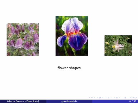
Discontinuous PDEs

Growth with obstacles yields a PDE with discontinuous right hand side

Ω Ω Ω

γ(t )1

γ(t )3γ(t )2

(can be modeled by a differential inclusion)


Well-posedness of the stem growth model with obstacle(A.B. - M.Palladino, work in progress)

Solutions exist and are unique except if a (highly non-generic) breakdownconfiguration occurs

good

ΩΩ

bad badgood

ΩΩ




Vines clinging to tree branches (A.B., M.Palladino, W.Shen)

add a term which bends the stem toward the obstacle, at points which aresufficiently close (i.e., at a distance < δ0 from the obstacle)

(t,s)α

0s

η(s)

δ

δ0

Ω

P(t,s)

k(t,s)

⊥k

ψ(x).

= η(d(x ,Ω)

)In the case of a vine that clings to a branch of another tree, the evolutionequation contains an additional term (=⇒ bending toward the obstacle)

∂

∂tk(t, s) = · · · +

(∫ s

0

e−β(t−σ)⟨∇ψ(P(t, σ)) , k⊥(t, σ)

⟩dσ

)k⊥(t, s)


Numerical simulations (Wen Shen)


A system of PDEs modeling controlled growth in Rn

To grow into a specific shape, different portions of the living tissue mustexpand at different rates. This can be achieved by a chemical gradient.

The system of PDEs should include:

(1) One or more diffusion equations, describing the density of growth-inducingnutrients/morphogens inside the living tissue

(2) A dynamic equation, describing how particles on the tissue move, as a resultof bulk growth

v

(t)

v

Ω


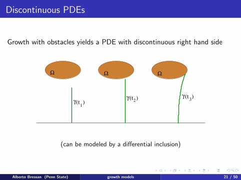
A linear diffusion-adsorption equation

Ω(t) = region occupied by living tissue at time t

w(t, x) density of (morphogen-producing) signaling cells, at time t, at point x ∈ Ω(t)

uτ = w + ∆u − u x ∈ Ω(t)

∇u · n = 0 x ∈ ∂Ω(t)

u = density of growth-inducing chemical. Determined by

production + diffusion + adsorption

Diffusion of chemicals within the living tissue is much faster than the growth of thetissue itself

By separation of time scales, it is appropriate to consider the steady stateu −∆u = w x ∈ Ω(t)

∇u · n = 0 x ∈ ∂Ω(t)


The growth equations

v(t, x) = velocity determined by bulk growth

Uniquely determined (up to a rigid motion) by the variational problem minimize: E (v).

=1

2

∫Ω(t)|sym∇v|2 dx

subject to: div v = u

E (v) = elastic energy of the infinitesimal deformation

symA.

=A + AT

2, skewA

.=

A− AT

2


The growth equations

Finally, we assume that morphogen-producing cells are passively transportedwithin the tissue, so that

wt + div (wv) = 0 x ∈ Ω(t)

This has to be supplemented by assigning an initial domain and an initialdistribution of morphogen-producing cells:

Ω(0) = Ω0, w(0, ·) = w0

v

(t)

v

Ω


Summary of the equations

Density of morphogen

u = argmin

∫Ω

( |∇u|22

+u2

2−wu

)dx ⇐⇒

u −∆u = w x ∈ Ω

∇u · n = 0 x ∈ ∂Ω

Velocity field determined by bulk growth

v = argmin

∫Ω

|sym∇v|2 dx

subject to: div v = u

⇐⇒

−∆v + 2∇p = ∇u x ∈ Ω

div v = u x ∈ Ω

(sym∇v − pI)n = 0 x ∈ ∂Ω

Density of morphogen-producing cells

wt + div (vw) = 0


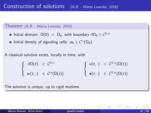
Construction of solutions (A.B. - Marta Lewicka, 2016)

Theorem (A.B. - Marta Lewicka, 2016)

Initial domain: Ω(0) = Ω0, with boundary ∂Ω0 ∈ C2,α

Initial density of signaling cells: w0 ∈ Cα(Ω0).

A classical solution exists, locally in time, with ∂Ω(t) ∈ C2,α

w(t, ·) ∈ Cα(Ω(t))

u(t, ·) ∈ C2,α(Ω(t))

v(t, ·) ∈ C2,α(Ω(t))

The solution is unique, up to rigid motions.


Main steps of the proof:

Represent the moving of the growing set by a function ϕ : Σ 7→ R

(x)n

n

x ΩϕΣ

x+ ϕ

Ω

Discretize time: tk = kε.Given Ωk , wk , the inductive time step consists of three parts:

(1) Solve the elliptic equation for the morphogen density u(production + diffusion + absorption)

minimize:

∫Ωk

( |∇u|22

+u2

2− wku

)dx


(2) Find the velocity v as minimizer of

E [v] =1

2

∫Ωk

|sym∇v|2 dx subject to: div v = u

Korn inequality =⇒ existence of v, unique under the additional constraints∫Ωk

v dx = 0, skew

∫Ωk

∇v dx = 0

(3) update the domain Ω and the density w of signaling cells

Ωk+1 = x + εv(x) ; x ∈ Ωk

wk+1(x + εv(x)).

=wk(x)

det(I + ε∇v(x))


ε

v

v

Ω(t+ )

(t)Ω

Schauder-type estimates by Agmon-Douglis-Nirenberg (1964)=⇒ C2,α regularity of approximate solutions uk , vk , and of theboundary ∂Ωk , uniformly for t ∈ [0,T ], with T independent of ε

regularity =⇒ compactness =⇒ convergence to a limit solution asε→ 0 (for a subsequence)


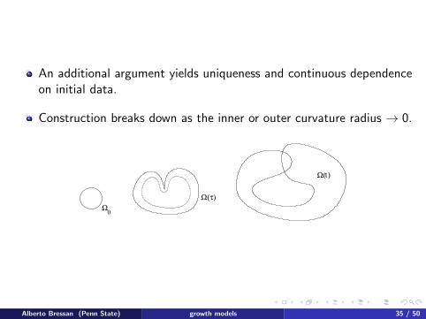
An additional argument yields uniqueness and continuous dependenceon initial data.

Construction breaks down as the inner or outer curvature radius → 0.

Ω( )

Ω(τ)

Ω0

t


Shapes

The shape of a set is its equivalence class modulo

rotations and translations: x 7→ Rx + a

homothetic rescalings: x 7→ λx , λ > 0

What kind of shapes can be produced by these controlled growth equations ?

Studying the limit of Ω(t) as t → +∞ is NOT meaningful


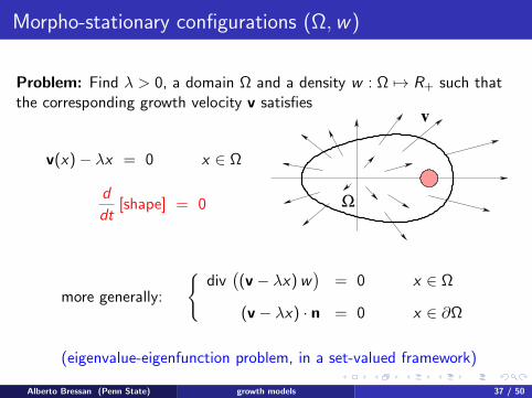
Morpho-stationary configurations (Ω,w)

Problem: Find λ > 0, a domain Ω and a density w : Ω 7→ R+ such thatthe corresponding growth velocity v satisfies

v(x)− λx = 0 x ∈ Ω

d

dt[shape] = 0 Ω

v

more generally:

div((v − λx)w

)= 0 x ∈ Ω

(v − λx) · n = 0 x ∈ ∂Ω

(eigenvalue-eigenfunction problem, in a set-valued framework)


How to break away from radial symmetry?

Turing instability

requires at least two components (u1, u2), diffusing at different rates

produces periodic patterns

Stratified domains

the growing domain M = M1 ∪ · · · ∪Mn is the union of manifolds ofdifferent dimensions

Different topologies should give raise to different morpho-stationaryconfigurations


Does each (topological) equivalence class of stratified domains yield afinite-parameter family of morpho-stationary configurations?

~

M

M

M

M

M

~

~

1

2

3

2

3

1

M


Constructing a morpho-stationary configuration

Linear Algebra: to find the largest positive eigenvector of a matrix A, fixv0 ∈ Rn take the limit of the iterates

vk+1 =Avk|Avk |

To construct a morpho-stationary configuration:

solve the dynamic evolution equation, adding a rescaling term that keeps thediameter of the domain constant

let t → +∞, prove that a nonsingular limit is achieved


Basic parameters

M

1

2

3

M

M

diffusion, adsorption coefficients on the 1-D manifold M1

diffusion, adsorption coefficients on the 2-D manifolds M2,M3

length growth rate on M1

area growth rate on M2,M3



0 0.2 0.4 0.6 0.8 1-0.5

-0.4

-0.3

-0.2

-0.1

0

0.1

0.2

0.3

0.4

0.5time=11.60

area growth rate << elongation rate


0 0.2 0.4 0.6 0.8 1-0.5

-0.4

-0.3

-0.2

-0.1

0

0.1

0.2

0.3

0.4

0.5time=20.00


-0.2 0 0.2 0.4 0.6 0.8 1-0.8

-0.6

-0.4

-0.2

0

0.2

0.4

0.6

0.8time=20.00


area growth rate >> elongation rate


Further directions . . .

Solve the linear system of PDEs for the velocity v constructing a Greenfunction.

Using the Green function, give a direct proof of regularity, without relying onAgmon-Douglis-Nirenberg’s theorem.

Extend the existence-uniqueness result to the case of a growing stratifieddomain (requires: estimates on domains with corners)


Anisotropic diffusion and stress-strain response

=⇒ additional ways to produce non radially symmetric shapes


Growth of curved surfaces in R3


Growth of Stem + Branches

Introduce rules for

initiation of new branches

growth and bending of branches

Is there a feedback “stabilizing” the growth of trunk + branchestoward a particular tree shape?


Conclusions . . .

Interesting shapes can be obtained fromeigenvalue-eigenfunction problems in a set-valued framework(morpho-stationary configurations on stratified domains)

Control & Stabilization of Growth Equationswill provide a rich source of mathematical problems


Documents

PDE Models of Controlled Biological Growth · PDF filePDE Models of Controlled Biological Growth ... How can Nature control growth, ... density of (morphogen-producing)