PDE methods for Image Segmentation and Shape Analysis:From the Brain to the Prostate and Backpresented by John Melonakos – NAMIC Core 1 Workshop – 30/May/2007

2

Outline

Bhattacharyya Segmentation

Segmentation Results--------------------------------------- Shape Analysis

Shape-Driven Segmentation

3

Contributors

Georgia Tech- Yogesh Rathi, Sam

Dambreville, Oleg Michailovich, Jimi Malcolm, Allen Tannenbaum

4

Publications

S. Dambreville, Y. Rathi, and A. Tannenbaum. A framework for Image Segmentation using Shape Models and Kernel Space Shape Priors. IEEE Transactions on Pattern Analysis and Machine Intelligence, (to appear 2007).

O. Michailovich, Y. Rathi, and A. Tannenbaum. Image Segmentation using Active Contours Driven by Informaion-Based Criteria. IEEE Transactions on Image Processing, (to appear 2007).

Y. Rathi, O. Michailovich, and A. Tannenbaum. Segmenting images on the Tensor Manifold. In CVPR, 2007.

Eric Pichon, Allen Tannenbaum, and Ron Kikinis. A statistically based surface evolution method for medical image segmentation: presentation and validation. In International Conference on Medical Image Computing and Computer Assisted Intervention (MICCAI), volume 2, pages 711-720, 2003. Note: Best student presentation in image segmentation award.

Y. Rathi, O. Michailovich, J. Malcolm, and A. Tannenbaum. Seeing the Unseen: Segmenting with Distributions. In Intl. Conf. Signal and Image Processing, 2006.

J. Malcolm, Y. Rathi, A. Tannenbaum. Graph cut segmentation with nonlinear shape priors. In Intl. Conf. Signal and Image Processing, 2007.

5

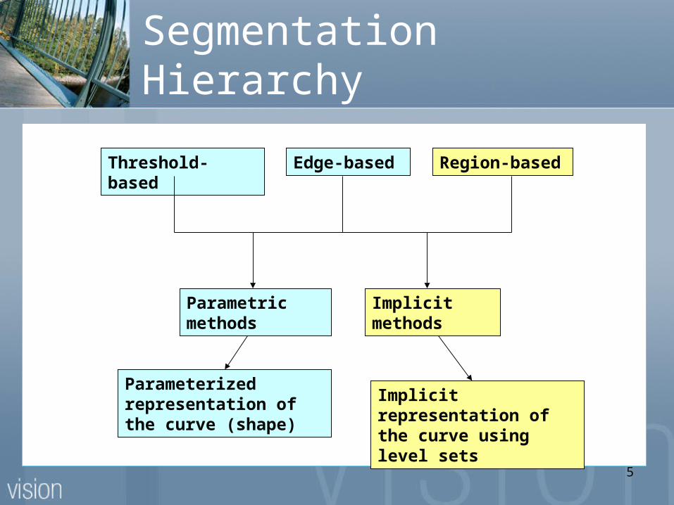
Segmentation Hierarchy

Threshold-based

Edge-based

Region-based

Parametric methods

Implicit methods

Parameterized representation of the curve (shape)

Implicit representation of the curve using level sets

6

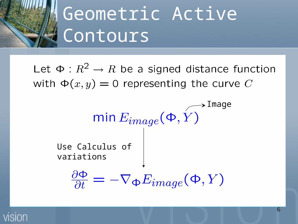
Geometric Active Contours

Image

Use Calculus of variations

7

Our Contributions

Segmentation by separating intensity based probability distributions (not just intensity moments as in previous works).

Novel formulation of the Bhattacharyya distance in the level set framework so as to optimally separate the region inside and outside the evolving contour.

8

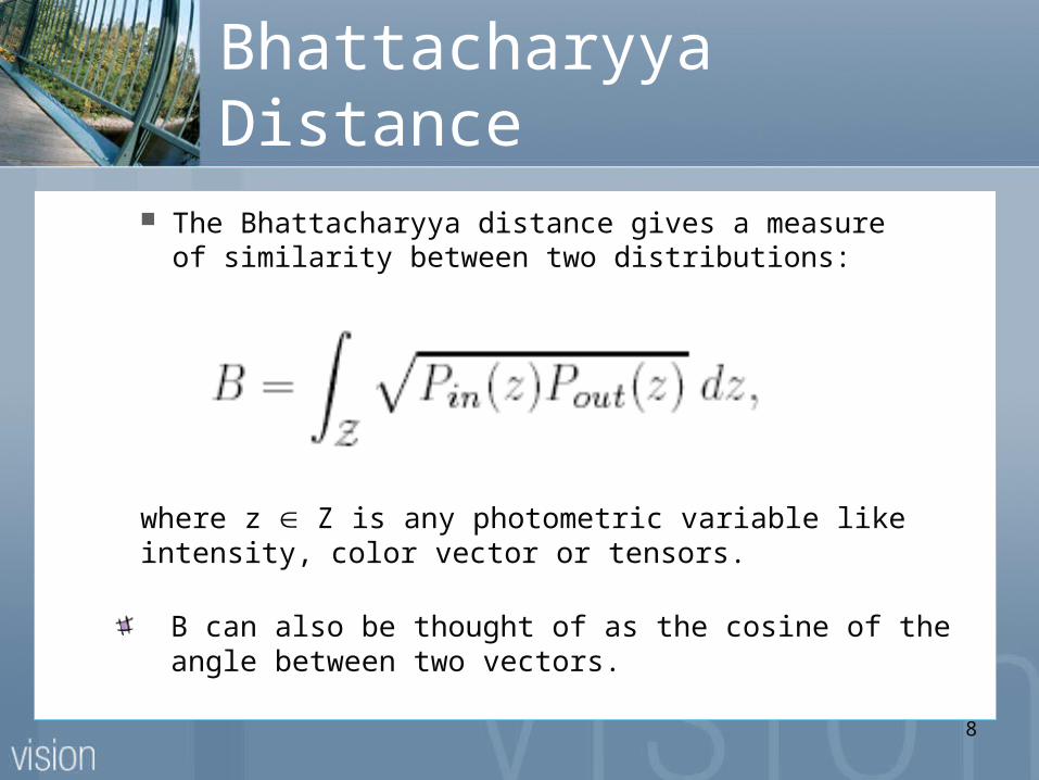
Bhattacharyya Distance

The Bhattacharyya distance gives a measure of similarity between two distributions:

where z Z is any photometric variable like intensity, color vector or tensors.

B can also be thought of as the cosine of the angle between two vectors.

9

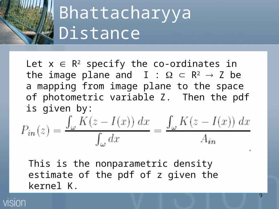
Bhattacharyya Distance

Let x R2 specify the co-ordinates in the image plane and I : R2 Z be a mapping from image plane to the space of photometric variable Z. Then the pdf is given by:

This is the nonparametric density estimate of the pdf of z given the kernel K.

10

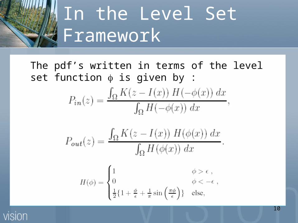
In the Level Set Framework

The pdf’s written in terms of the level set function is given by :

11

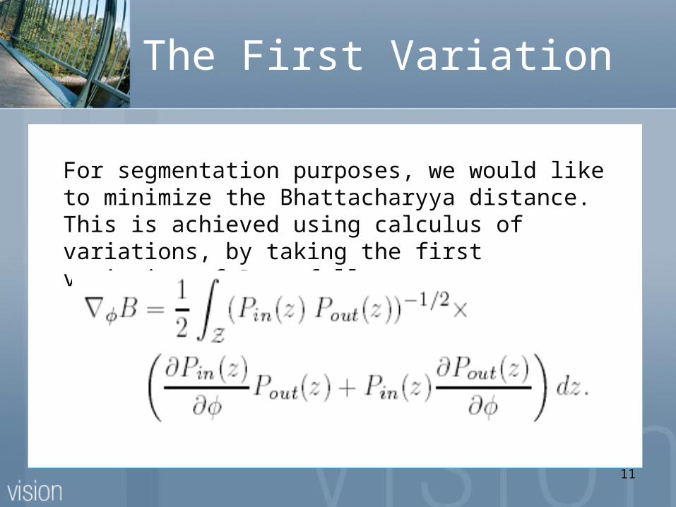
The First Variation

For segmentation purposes, we would like to minimize the Bhattacharyya distance. This is achieved using calculus of variations, by taking the first variation of B as follows :

12

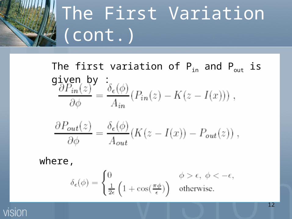
The First Variation (cont.)

The first variation of Pin and Pout is given by :

where,

13

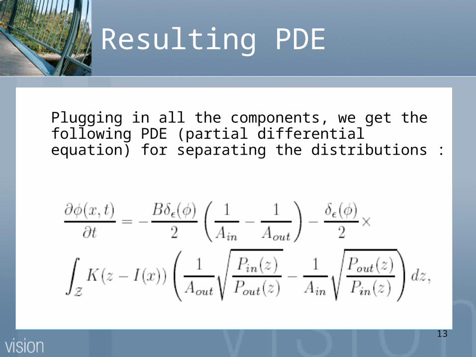
Resulting PDE

Plugging in all the components, we get the following PDE (partial differential equation) for separating the distributions :

14

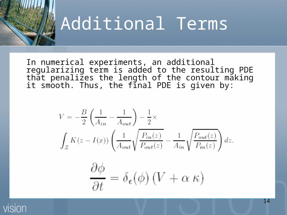
Additional Terms

In numerical experiments, an additional regularizing term is added to the resulting PDE that penalizes the length of the contour making it smooth. Thus, the final PDE is given by:

15

Outline

Bhattacharyya Segmentation

Segmentation Results--------------------------------------- Shape Analysis

Shape-Driven Segmentation

16

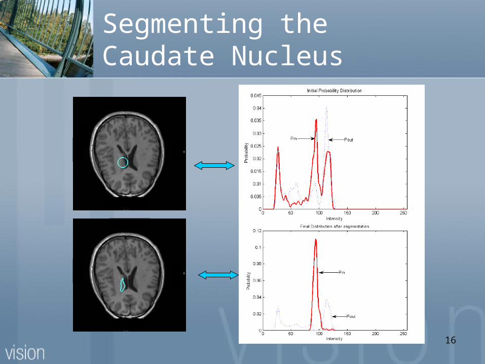
Segmenting the Caudate Nucleus

17

Caudate Nucleus

18

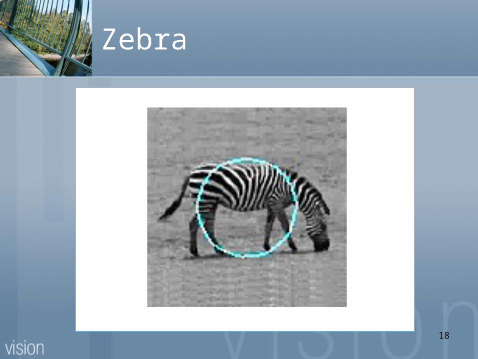
Zebra

19

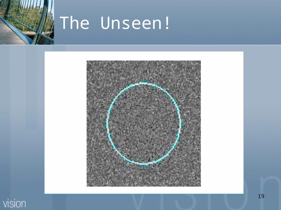
The Unseen!

20

The Unseen!

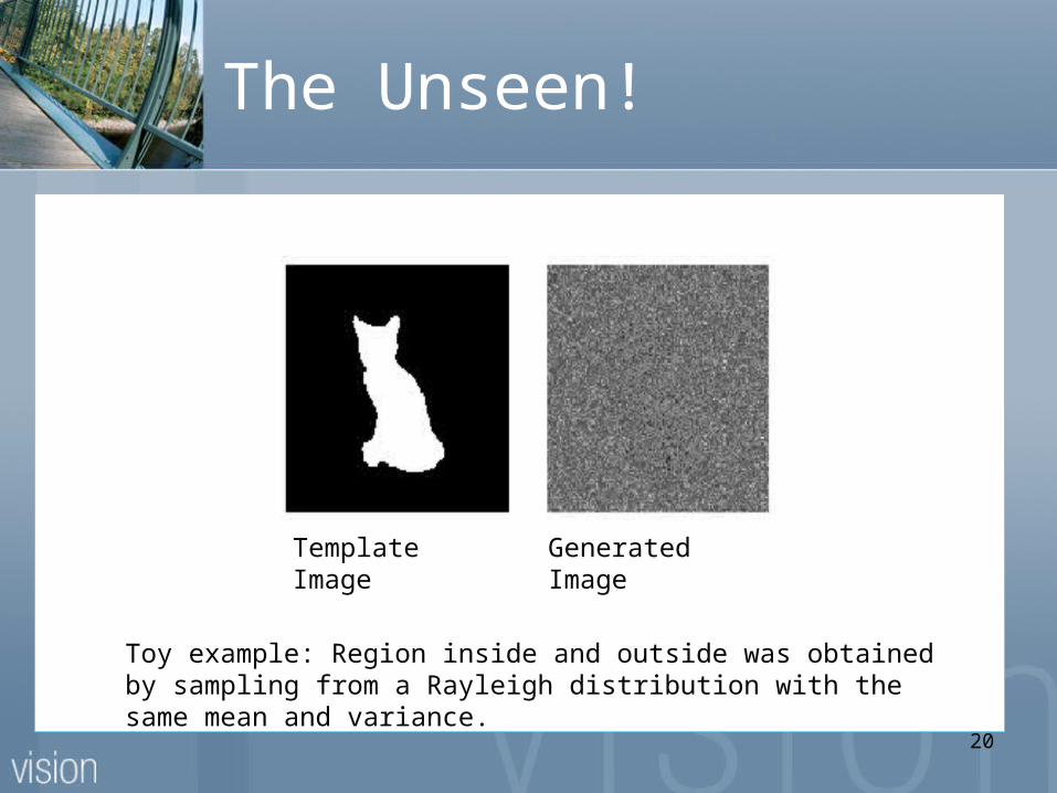
Toy example: Region inside and outside was obtained by sampling from a Rayleigh distribution with the same mean and variance.

Template Image

Generated Image

21

The Unseen!

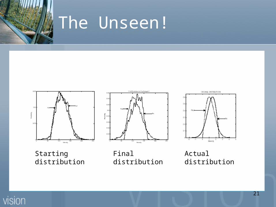
Starting distribution Final distribution Actual distribution

22

Application to Tensors

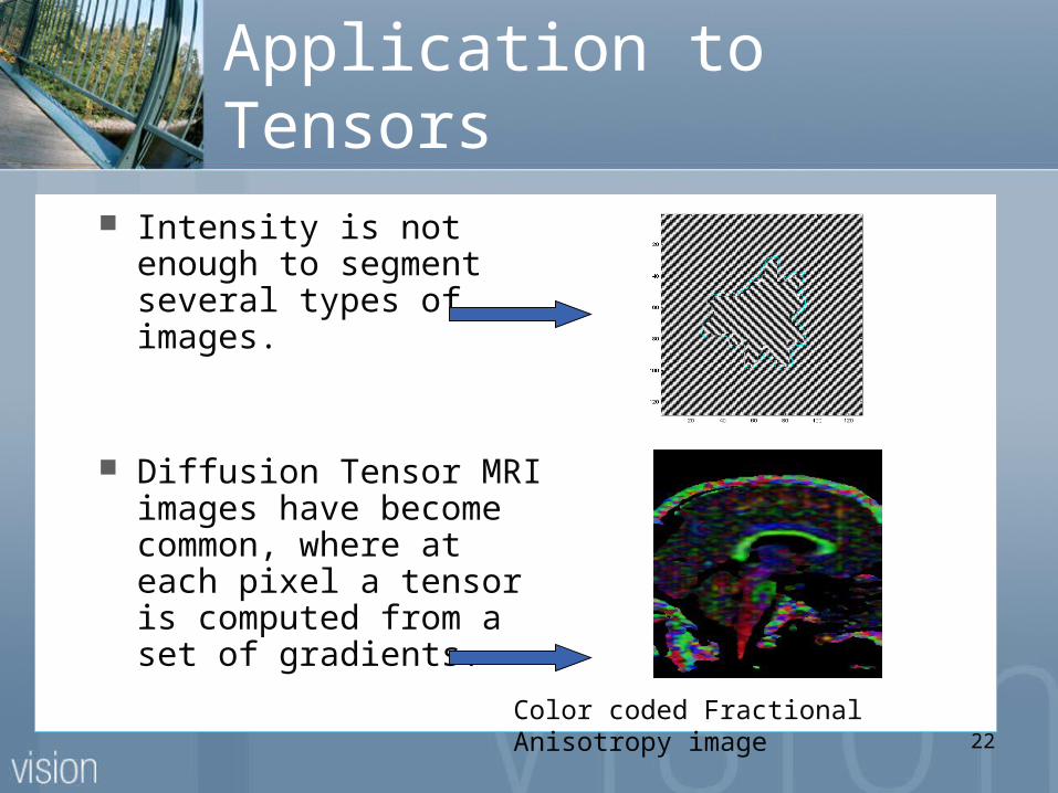
Intensity is not enough to segment several types of images.

Diffusion Tensor MRI images have become common, where at each pixel a tensor is computed from a set of gradients.

Color coded Fractional Anisotropy image

23

Structure Tensors

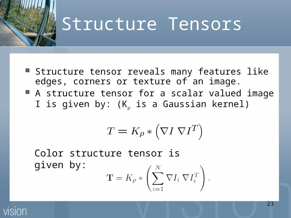
Structure tensor reveals many features like edges, corners or texture of an image.

A structure tensor for a scalar valued image I is given by: (K is a Gaussian kernel)

Color structure tensor is given by:

24

The Tensor Manifold

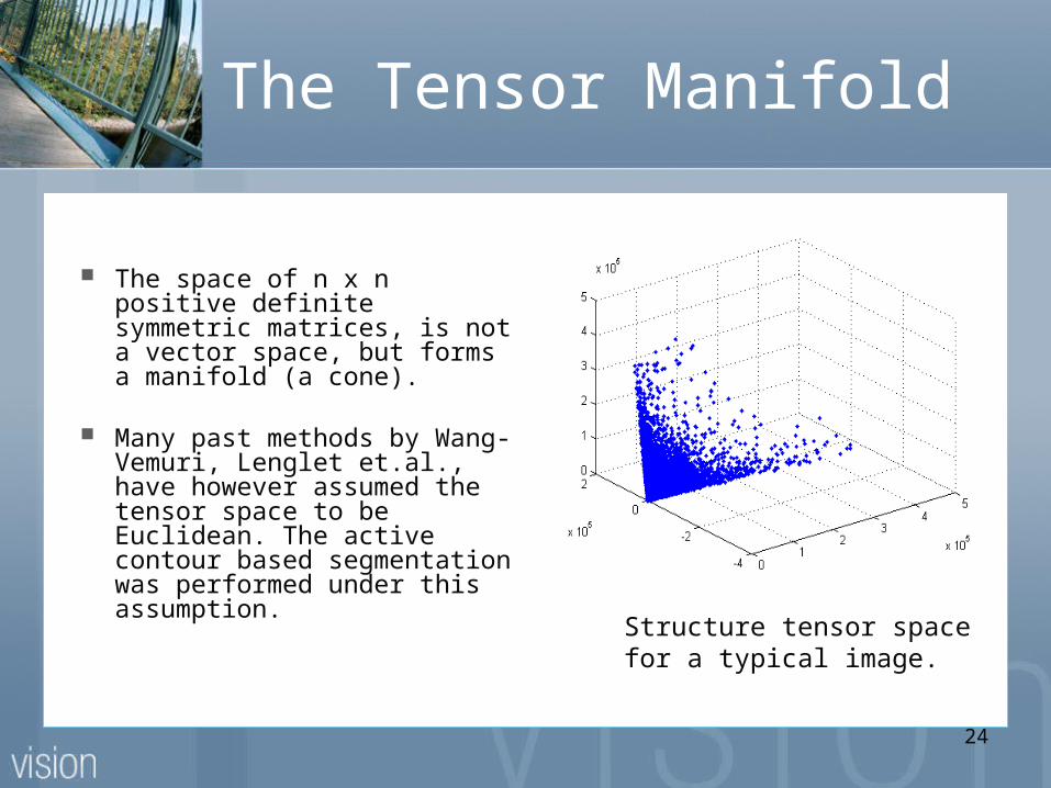
The space of n x n positive definite symmetric matrices, is not a vector space, but forms a manifold (a cone).

Many past methods by Wang-Vemuri, Lenglet et.al., have however assumed the tensor space to be Euclidean. The active contour based segmentation was performed under this assumption. Structure tensor space for

a typical image.

25

Riemannian vs Euclidean Manifold

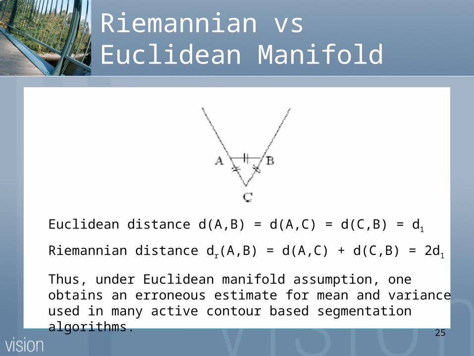
Euclidean distance d(A,B) = d(A,C) = d(C,B) = d1

Riemannian distance dr(A,B) = d(A,C) + d(C,B) = 2d1

Thus, under Euclidean manifold assumption, one obtains an erroneous estimate for mean and variance used in many active contour based segmentation algorithms.

26

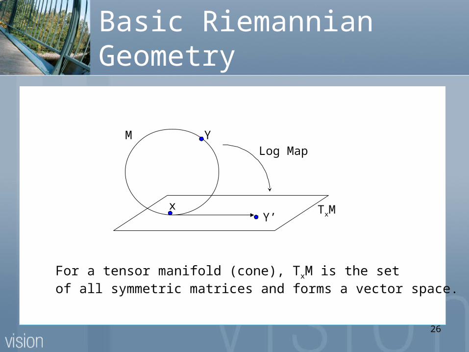
Basic Riemannian Geometry

For a tensor manifold (cone), TxM is the setof all symmetric matrices and forms a vector space.

TxMx

Y

Y’

Log Map M

27

Tensor Space

A recent method proposed by Lenglet et.al. (2006), incorporates the Riemannian geometry of the tensor space and performs segmentation by assuming a Gaussian distribution of the object and background.

By using the Bhattacharyya distance and taking into account the Riemannian structure of the tensor manifold, we propose to extend the above segmentation technique to any arbitrary and non-analytic probability distribution.

28

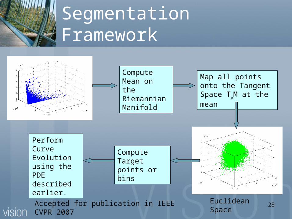
Segmentation Framework

Compute Mean on the Riemannian Manifold

Map all points onto the Tangent Space TM at the mean

Euclidean Space

Compute Target points or bins

Perform Curve Evolution using the PDE described earlier.

Accepted for publication in IEEE CVPR 2007

29

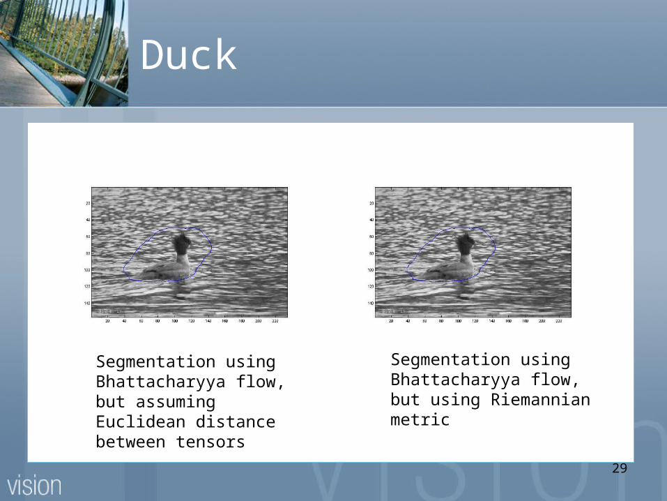
Duck

Segmentation using Bhattacharyya flow, but using Riemannian metric

Segmentation using Bhattacharyya flow, but assuming Euclidean distance between tensors

30

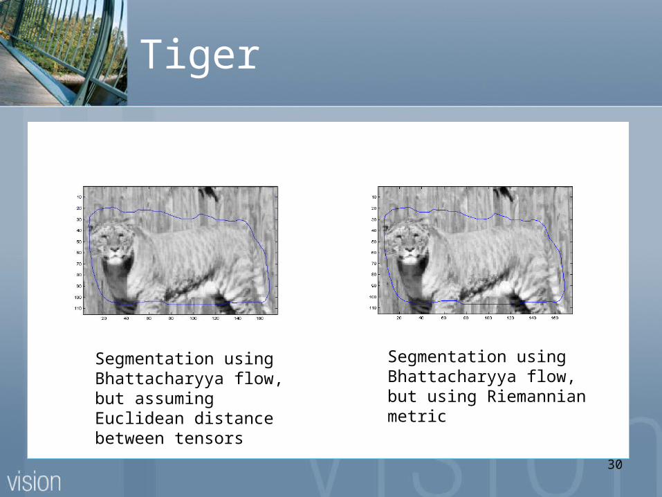
Tiger

Segmentation using Bhattacharyya flow, but assuming Euclidean distance between tensors

Segmentation using Bhattacharyya flow, but using Riemannian metric

31

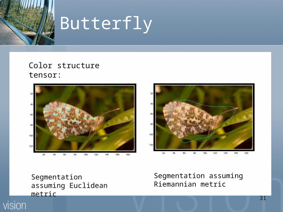
Butterfly

Segmentation assuming Euclidean metric

Segmentation assuming Riemannian metric

Color structure tensor:

32

Segmentation Summary

No assumption on the distribution of the object or background.

Computationally very fast, since we only need to update the probability distribution instead of having to map each point in the image from Riemannian space to tangent space after each iteration to compute the mean and variance (under a Gaussian assumption).

33

Outline

Bhattacharyya Segmentation

Segmentation Results--------------------------------------- Shape Analysis

Shape-Driven Segmentation

34

Contributors

Georgia Tech- Delphine Nain, Xavier

LeFaucheur, Yi Gao, Allen Tannenbaum

35

Publications

D. Nain, S. Haker, A. Tannenbaum. Multiscale 3D shape representation and segmentation using spherical wavelets. IEEE Trans. Medical Imaging, 26 (2007). pp 598-618.

D. Nain, S. Haker, A. Bobick, and A. Tannenbaum. Shape-Driven 3D Segmentation using using Spherical Wavelets. In Proceedings of MICCAI, Copenhagen, 2006. Note: Best Student Paper Award in the category Segmentation and Registration.

D. Nain, S. Haker, A. Bobick, and A. Tannenbaum. Multiscale 3D Shape Analysis using Spherical Wavelets. In Proceedings of MICCAI, Palm Springs, 2005.

36

Overview

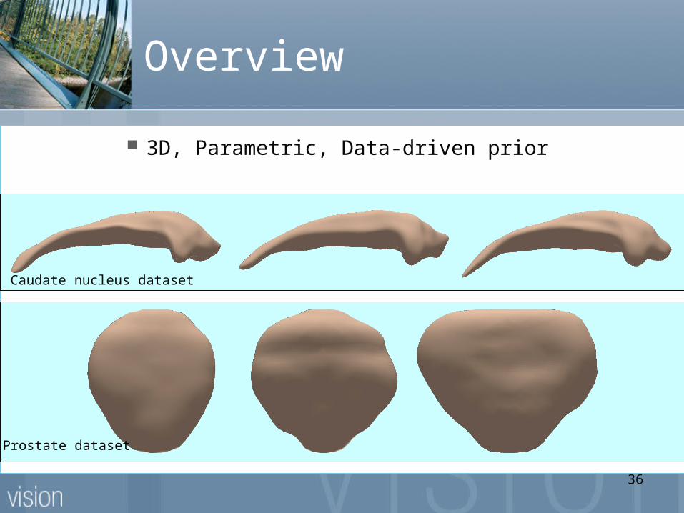
3D, Parametric, Data-driven prior

Caudate nucleus dataset

Prostate dataset

37

Overview of ASM

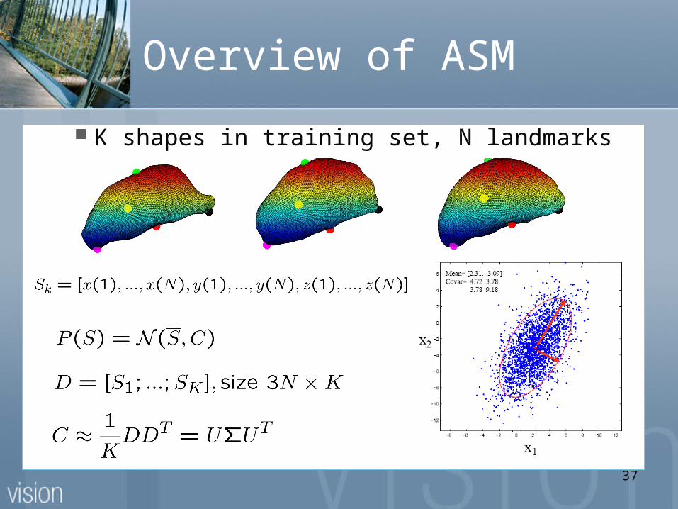
K shapes in training set, N landmarks

38

Limitations of ASM

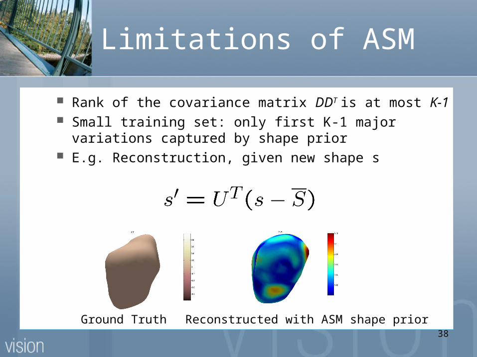
Rank of the covariance matrix DDT is at most K-1 Small training set: only first K-1 major variations

captured by shape prior E.g. Reconstruction, given new shape s

Ground Truth Reconstructed with ASM shape prior

39

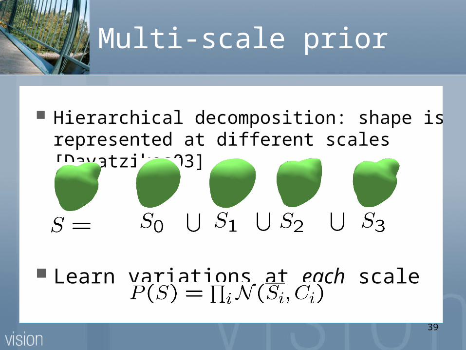
Multi-scale prior

Hierarchical decomposition: shape is represented at different scales [Davatzikos03]

Learn variations at each scale

40

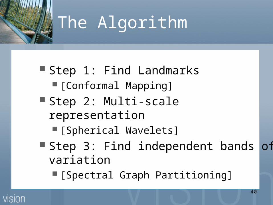
The Algorithm

Step 1: Find Landmarks [Conformal Mapping]

Step 2: Multi-scale representation [Spherical Wavelets]

Step 3: Find independent bands of variation [Spectral Graph Partitioning]

41

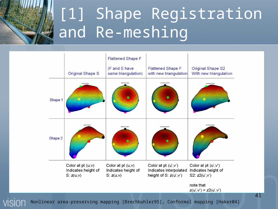
[1] Shape Registration and Re-meshing

Nonlinear area-preserving mapping [Brechbuhler95], Conformal mapping [Haker04]

42

[2] Spherical Wavelets

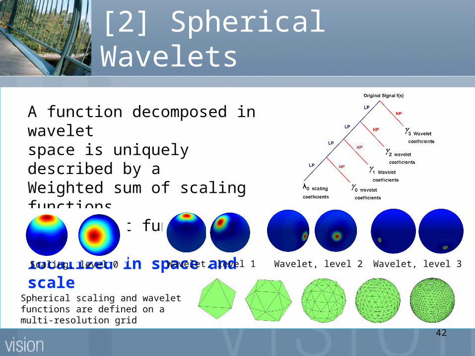
A function decomposed in waveletspace is uniquely described by a Weighted sum of scaling functions and wavelet functions that are localized in space and scale

Spherical scaling and wavelet functions are defined on a multi-resolution grid

Scaling, level 0 Wavelet, level 1 Wavelet, level 2 Wavelet, level 3

43

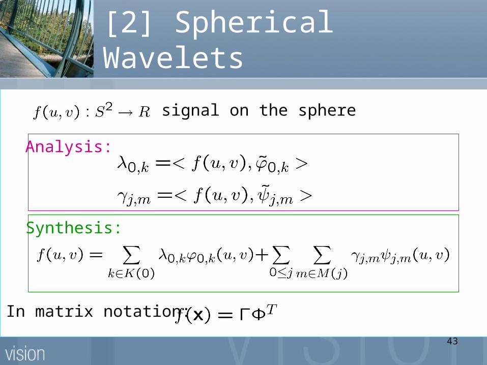
[2] Spherical Wavelets

In matrix notation:

is signal on the sphere

Analysis:

Synthesis:

44

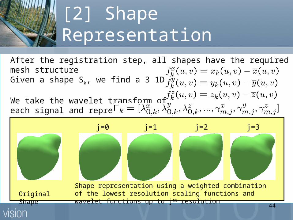
[2] Shape Representation

After the registration step, all shapes have the required mesh structureGiven a shape Sk, we find a 3 1D signals:

We take the wavelet transform of each signal and represent the shape as:

Original ShapeShape representation using a weighted combination of the lowest resolution scaling functions and wavelet functions up to jth resolution

j=0 j=1 j=2 j=3

45

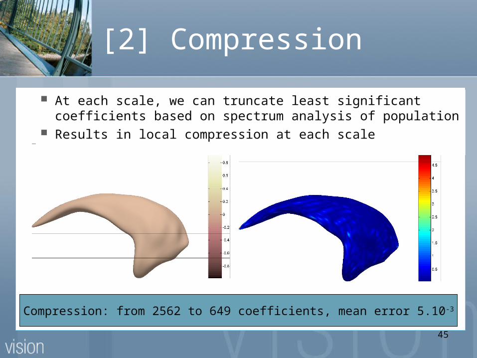
[2] Compression

Compression: from 2562 to 649 coefficients, mean error 5.10-3

At each scale, we can truncate least significant coefficients based on spectrum analysis of population

Results in local compression at each scale

46

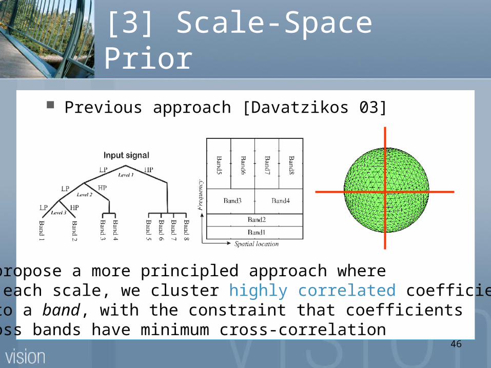
[3] Scale-Space Prior

Previous approach [Davatzikos 03]

We propose a more principled approach wherefor each scale, we cluster highly correlated coefficients into a band, with the constraint that coefficients across bands have minimum cross-correlation

47

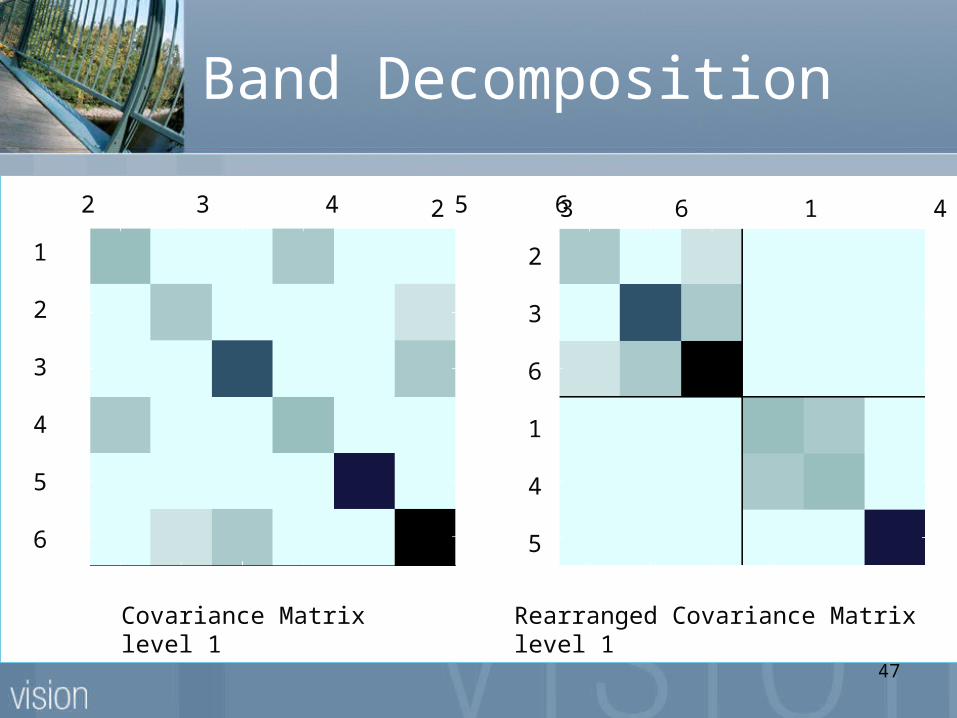
Band Decomposition

Covariance Matrixlevel 1

1 2 3 4 5 6

1

2

3

4

5

6

2 3 6 1 4 5

2

3

6

1

4

5

Rearranged Covariance Matrixlevel 1

48

Band Decomposition

Spectral Graph Partitioning technique [Shi00]

Fully connected graph G = (V,E) where nodes V are wavelet coefficients for a particular scale

Weight on each edge: w(i, j) is covariance between coefficients i and j

Stopping criterion: validating whether the subdivided band correspond to two independent distributions based on KL divergence

49

Band Decomposition

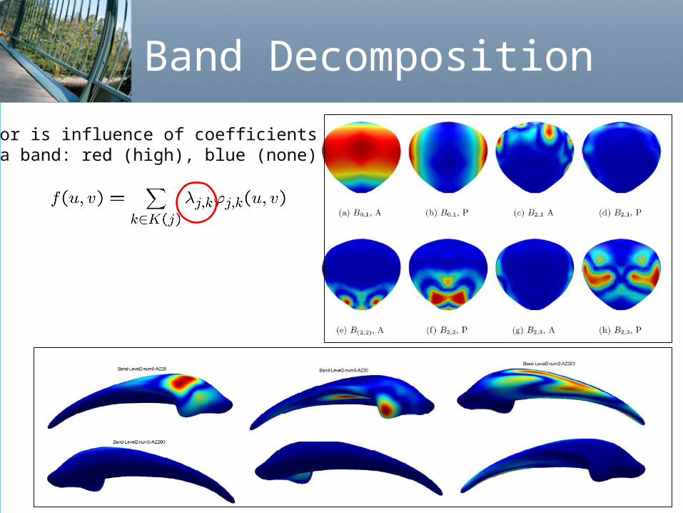
Color is influence of coefficients in a band: red (high), blue (none)

50

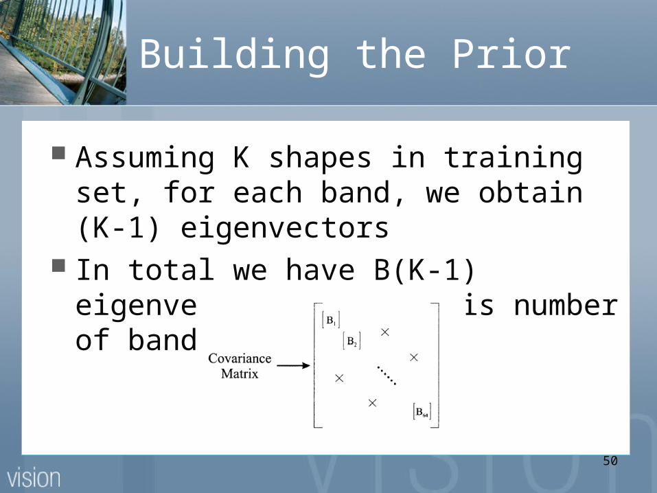
Building the Prior

Assuming K shapes in training set, for each band, we obtain (K-1) eigenvectors

In total we have B(K-1) eigenvectors, where B is number of bands

51

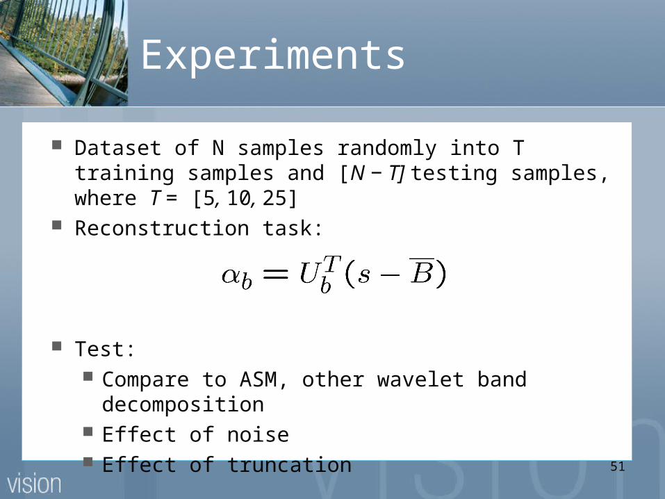
Experiments

Dataset of N samples randomly into T training samples and [N − T] testing samples, where T = [5, 10, 25]

Reconstruction task:

Test: Compare to ASM, other wavelet band

decomposition Effect of noise Effect of truncation

52

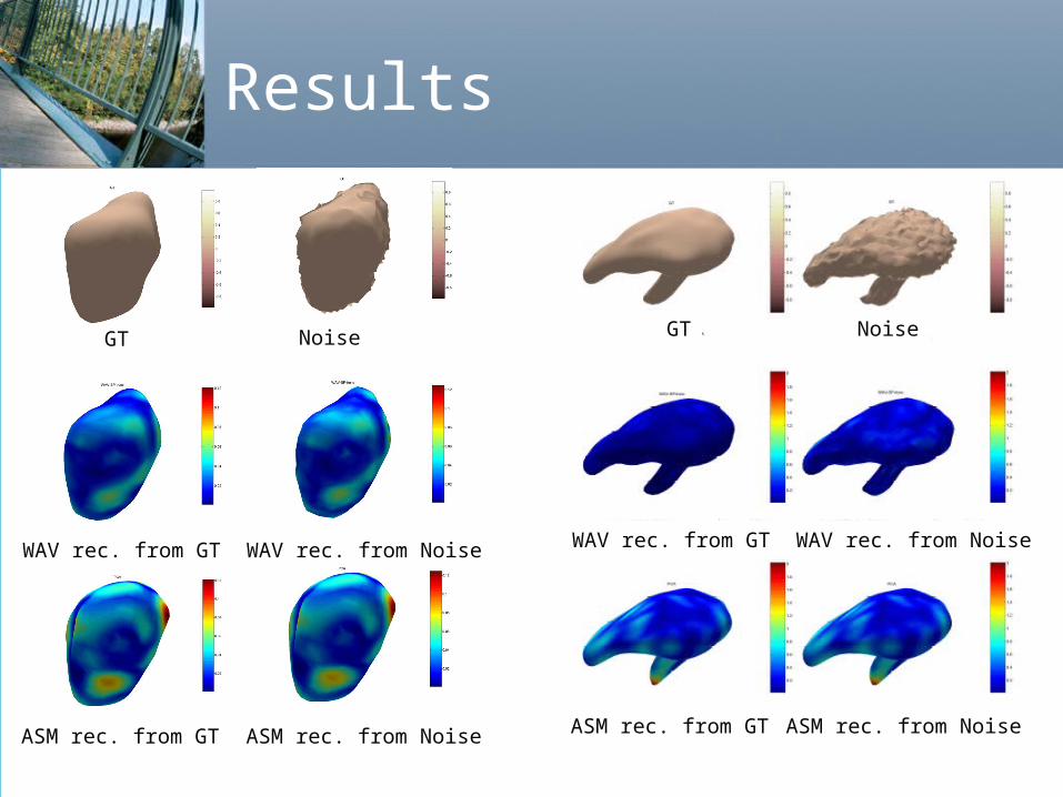
Results

GT Noise

WAV rec. from GT WAV rec. from Noise

ASM rec. from GT ASM rec. from Noise

GT Noise

WAV rec. from GT WAV rec. from Noise

ASM rec. from GT ASM rec. from Noise

53

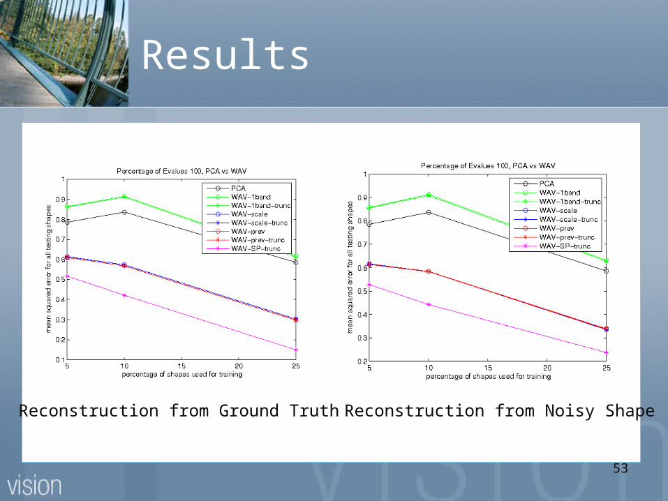
Results

Reconstruction from Ground Truth Reconstruction from Noisy Shape

54

Outline

Bhattacharyya Segmentation

Segmentation Results--------------------------------------- Shape Analysis

Shape-Driven Segmentation

55

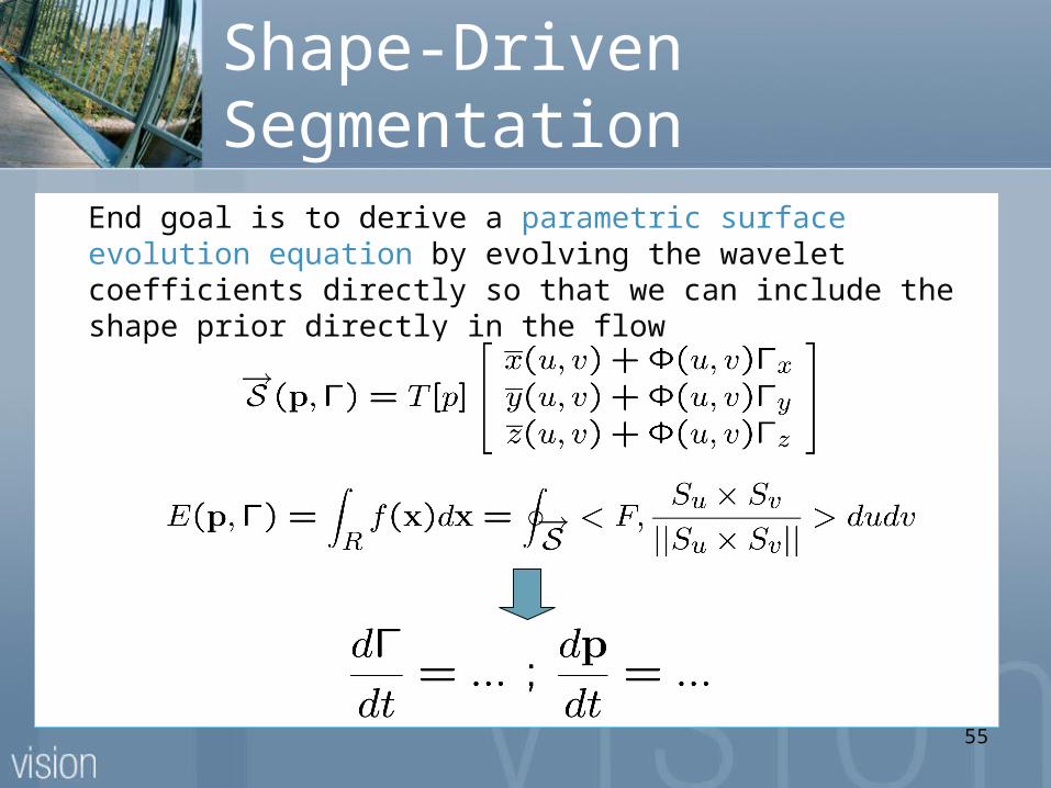
Shape-Driven Segmentation

End goal is to derive a parametric surface evolution equation by evolving the wavelet coefficients directly so that we can include the shape prior directly in the flow

56

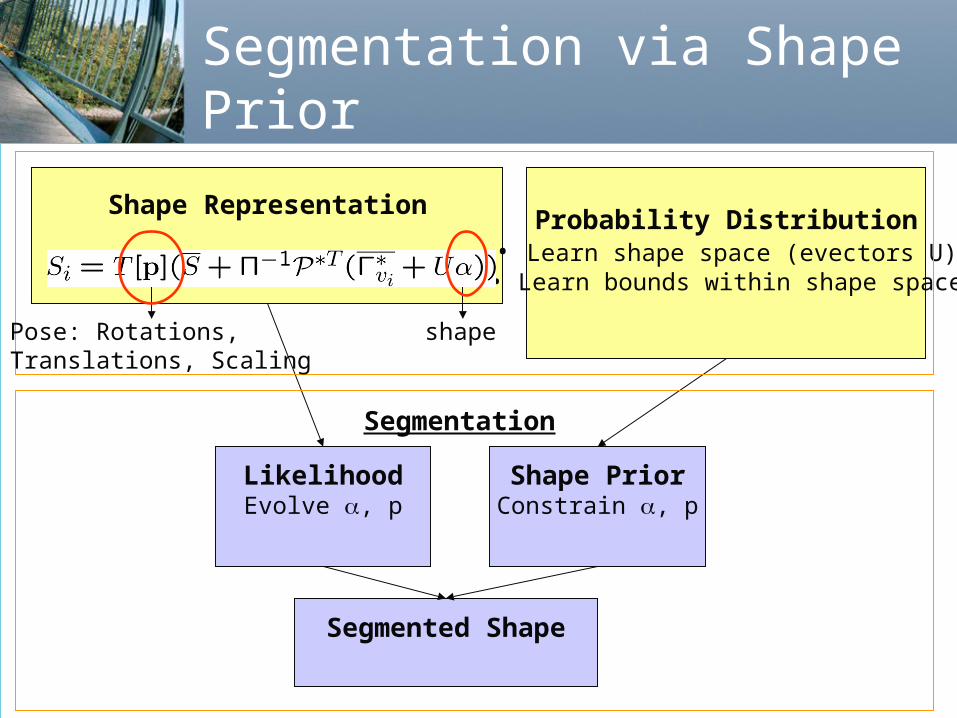
Segmentation via Shape Prior

LikelihoodEvolve , p

Shape Representation

Shape PriorConstrain , p

Segmented Shape

Segmentation

Probability Distribution• Learn shape space (evectors U)

• Learn bounds within shape space

Pose: Rotations,Translations, Scaling

shape

57

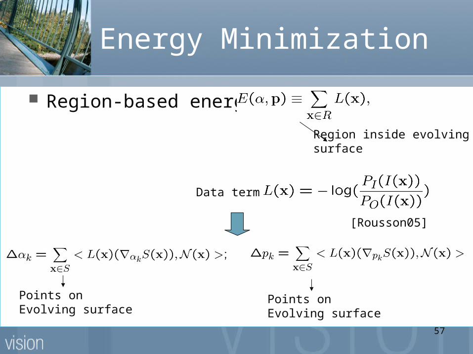
Energy Minimization

Region-based energy

Data term

Region inside evolvingsurface

[Rousson05]

Points onEvolving surface

Points onEvolving surface

58

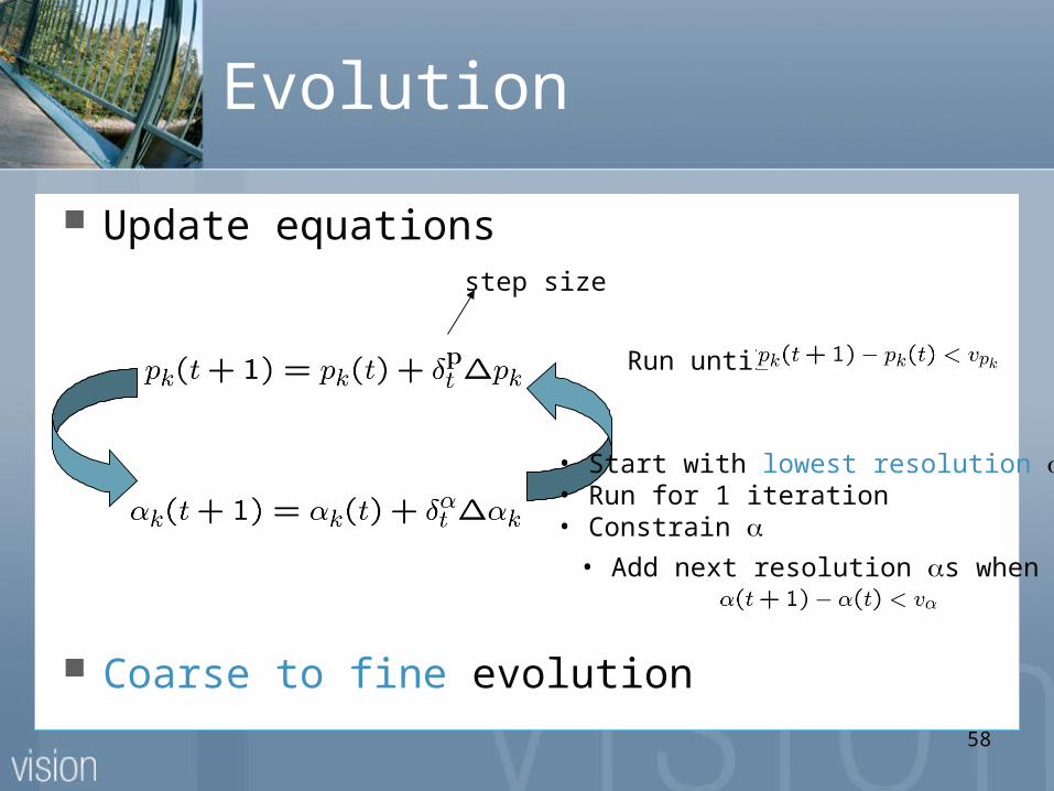
Evolution

Update equations

Run until

step size

• Start with lowest resolution s• Run for 1 iteration• Constrain • Add next resolution s when

Coarse to fine evolution

59

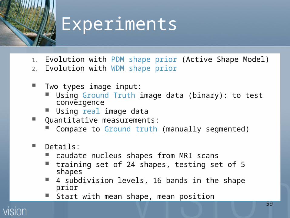
Experiments

1. Evolution with PDM shape prior (Active Shape Model)2. Evolution with WDM shape prior

Two types image input: Using Ground Truth image data (binary): to test

convergence Using real image data

Quantitative measurements: Compare to Ground truth (manually segmented)

Details: caudate nucleus shapes from MRI scans training set of 24 shapes, testing set of 5 shapes 4 subdivision levels, 16 bands in the shape prior Start with mean shape, mean position

60

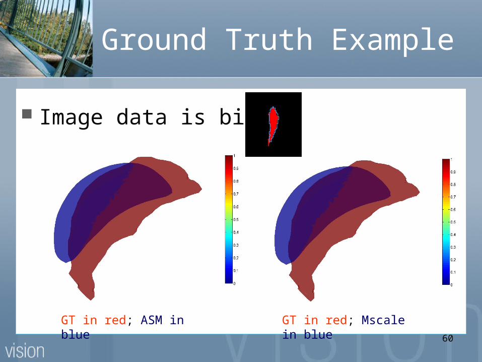
Ground Truth Example

Image data is binary

GT in red; ASM in blue GT in red; Mscale in blue

61

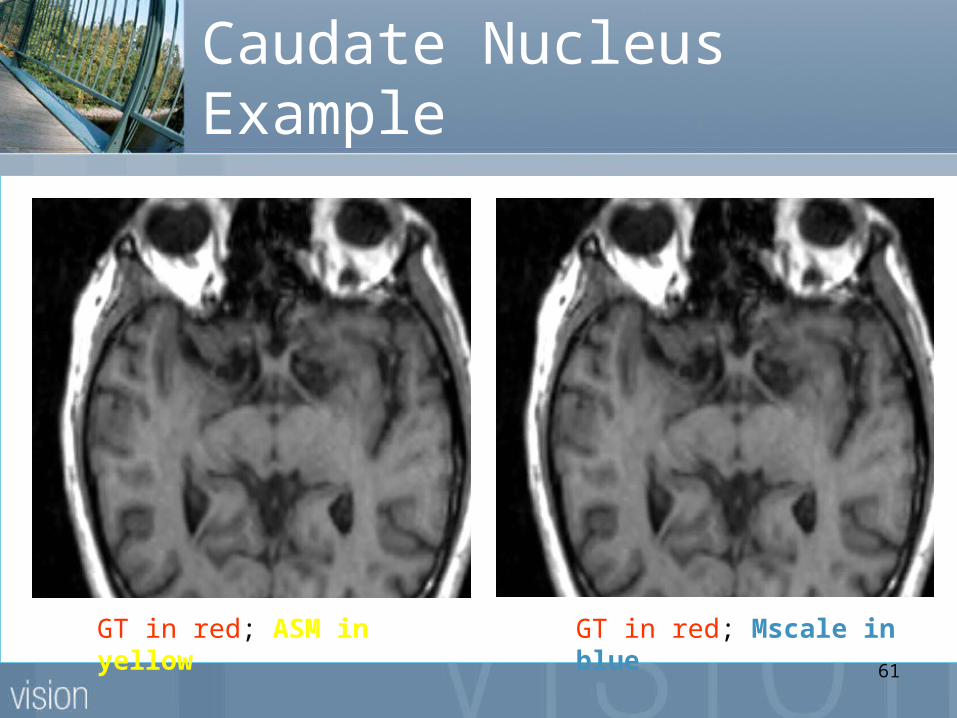
Caudate Nucleus Example

GT in red; ASM in yellow GT in red; Mscale in blue

62

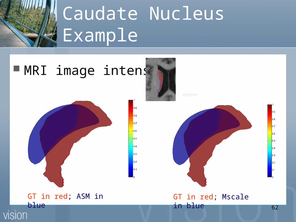
Caudate Nucleus Example

MRI image intensity

GT in red; ASM in blue GT in red; Mscale in blue

63

Conclusions (Speculations)

Geodesic tractography (tomorrow) Fast non-rigid registration (tomorrow)

Estimation and filtering techniques from tracking?

64

Questions?