Embed Size (px)
Citation preview
PC Passport
Spreadsheets Student Workbook
DRAFT November 2007

Published date: November 2007
Publication code: CB4122
Published by the Scottish Qualifications Authority
The Optima Building, 58 Robertson Street, Glasgow G2 8DQ
Ironmills Road, Dalkeith, Midlothian EH22 1LE
www.sqa.org.uk
The information in this publication may be reproduced to support the delivery of PC Passport
or its component Units. If it is to be used for any other purpose, then written permission must
be obtained from the Assessment Materials and Publishing Team at SQA. It must not be
reproduced for trade or commercial purposes.
© Scottish Qualifications Authority 2007
ii

Draft PC Passport Support Materials (November 2007)
Introduction This student workbook is one of a range of eight titles designed to cover
topics for the refreshed PC Passport. Each title in the range covers the
required subject material and exercises for candidates studying PC Passport.
This workbook covers all three levels of PC Passport — Beginner,
Intermediate and Advanced — with each level clearly identified.
There are a number of exercises associated with each subject and it is
recommended that centres download and use the sample exercise files
provided.
Each workbook will help prepare candidates for the assessments for the
refreshed PC Passport. It is recommended that centres use the most up-to-
date Assessment Support Packs appropriate for their type of centre, eg either
school, FE or work-based.
Spreadsheets Student Workbook — Beginner/Intermediate/Advanced iii

Draft PC Passport Support Materials (November 2007)
Spreadsheets Student Workbook — Beginner/Intermediate/Advanced iv

Draft PC Passport Support Materials (November 2007)
Contents Beginner 1 Spreadsheet Software 1 Excel Overview 1 Creating Workbooks 10
Exercise 1: Using Copy and Cut 16 Exercise 2: Using Copy and Paste 19 Exercise 3: Cell Formatting and Calculations 26 Exercise 4: Using Formulas 27 Exercise 5: Using AutoSum and Other Formatting Options 29
Cell Referencing 31 Exercise 6: Absolute/Relative Cell Referencing 34 Exercise 7: Absolute/Relative Cell Addressing and Statistical Functions 34
Formatting Text 35 Exercise 8: Formatting Cells 37 Exercise 9: Using AutoFormat 39
Previewing and Printing a Workbook 40 Exercise 10: Printing Your Workbook 45 Exercise 11: Working with Print Options 46
Using Functions 48 Intermediate 51 Mathematical Functions 52 Statistical Functions 53 Financial Functions 55 Logical Functions 57 Graphics 62 Charts 72
Exercise 12: Creating Charts 84 Exercise 13: Amending Charts 85
Advanced 87 File Protection 88
Exercise 14: Applying File Protection 95 Creating Spreadsheet Templates 96 Data Validation 98 Using Macros 104
Exercise 15: Creating a Macro 107 PivotTable Reports 108
Exercise 16: Using PivotTables 116 Using Goal Seek 116
Exercise 17: Using Scenarios 118 Sorting Data 119
Exercise 18: Sorting 121 Using Lists 121
Exercise 19: Using Lists 123 Using Filters 125
Exercise 20: Using Filters 129 Using Functions with Lists and Filters 132
Exercise 21: Using Lists, Data Forms and Filters 137 Finally 138
Spreadsheets Student Workbook — Beginner/Intermediate/Advanced v

Draft PC Passport Support Materials (November 2007)
Spreadsheets Student Workbook — Beginner/Intermediate/Advanced vi

Draft PC Passport Support Materials (November 2007)
Spreadsheet Software To enable you to perform calculations on numbers, hold lists of things,
perform analyses on data and create charts, you need to use spreadsheet
software. Spreadsheet software allows you to do all of these things and is the
most widely used software in any office, especially when you need to keep
financial information. There are two popular applications: Lotus 123 and
Microsoft Excel. You can also get specialist financial and accounting software
like SAGE.
Opening and Closing Spreadsheet Software You can open your spreadsheet software in a number of ways. The most
popular method is using the Start menu, which is shown at the bottom left of
the Windows screen on the taskbar:
♦ Click the Start button, choose All Programs (or Programs if you don’t
use Windows XP) and then Microsoft Excel or Lotus 123.
Note: If you use Windows XP, and you use Microsoft Excel frequently, you
may also find it on the menu shown when you first click the Start button. This
is to make it quicker for you to launch the program.
When you have finished using your spreadsheet software, you should close it.
You do this by clicking File on the menu bar and then choosing Exit from the
menu of options.
Excel Overview Microsoft Excel is one of the most popular spreadsheet applications, but most
have similar features to Excel. Files created in Excel are called workbooks. A
workbook may contain one or more worksheets.
Each worksheet in a workbook stores information in a grid of rows and
columns of cells. You can enter text, numbers, dates and calculations
(formulas) in the cells to present and analyse the information you need.
Spreadsheets Student Workbook — Beginner 1

Draft PC Passport Support Materials (November 2007)
For example, you could use a workbook to store budget forecasts, employee
timesheets, profit and loss accounts, calculation of depreciation, cash flow
analysis and monthly expense reports.
Some advantages of using a computer-based workbook are:
♦ You can format the information in a workbook using a variety of fonts, lines
and shading, making the information easier to read.
♦ Changes can be made to values in a workbook at any time, and all
calculations making reference to those values will be updated
automatically.
♦ The information in a workbook can be presented graphically using charts
of various types.
Each cell in the workbook has its own unique cell address (also known as the
cell reference). This is made up of its column letter and then its row number,
so the cell at the top left of the worksheet in column A on row 1 is cell A1. The
cell that reads ‘Expenditure’ in the above illustration is cell A12, while the cell
that reads ‘May’ is cell F5, and the active cell pointer is on cell A4.
Note: When working with Excel, you might notice that it sometimes inserts the
name of the worksheet the cell address comes from. In that case, in the
above example, cell H23 on sheet ‘Cash Flow Projections’ would be referred
to as:
‘Cash Flow Projections’!H23
Spreadsheets Student Workbook — Beginner 2
Draft PC Passport Support Materials (November 2007)
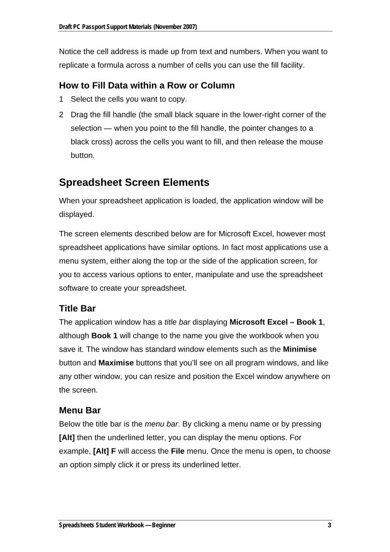
Notice the cell address is made up from text and numbers. When you want to
replicate a formula across a number of cells you can use the fill facility.
How to Fill Data within a Row or Column 1 Select the cells you want to copy.
2 Drag the fill handle (the small black square in the lower-right corner of the
selection — when you point to the fill handle, the pointer changes to a
black cross) across the cells you want to fill, and then release the mouse
button.
Spreadsheet Screen Elements When your spreadsheet application is loaded, the application window will be
displayed.
The screen elements described below are for Microsoft Excel, however most
spreadsheet applications have similar options. In fact most applications use a
menu system, either along the top or the side of the application screen, for
you to access various options to enter, manipulate and use the spreadsheet
software to create your spreadsheet.
Title Bar The application window has a title bar displaying Microsoft Excel – Book 1,
although Book 1 will change to the name you give the workbook when you
save it. The window has standard window elements such as the Minimise
button and Maximise buttons that you’ll see on all program windows, and like
any other window, you can resize and position the Excel window anywhere on
the screen.
Menu Bar Below the title bar is the menu bar. By clicking a menu name or by pressing
[Alt] then the underlined letter, you can display the menu options. For
example, [Alt] F will access the File menu. Once the menu is open, to choose
an option simply click it or press its underlined letter.
Spreadsheets Student Workbook — Beginner 3

Draft PC Passport Support Materials (November 2007)
Some commands can be accessed using keyboard shortcuts. When a
keyboard shortcut is available, you will see it described to the right of the
command name. For example, if you click the Edit menu, you will see the
Copy command can also be actioned by pressing [Ctrl] C. This means
pressing C while you hold down one of the [Ctrl] keys. Options that appear
dimmed are not available for selection at this time. If the command can also
be accessed through a toolbar button, eg Cut, the picture that appears on the
button is shown to the left of the menu option.
Initially, only some of the options will be shown on each menu, however, you
can extend the menu to show all the available options if necessary. As you
work with Excel, those options that you use will be added to the shortened list
initially displayed.
Toolbars To begin with, the Standard and Formatting toolbars are displayed — they are
the ones you work with most. You can choose to display or hide toolbars
using the View, Toolbars command. Alternatively, right-click any toolbar
currently displayed to see the shortcut menu and then select a toolbar name
to display or hide it.
Worksheet Tabs Each workbook in Excel is made up of one or more worksheets. Each
worksheet (or simply sheet) in the workbook is represented by a tab at the
bottom of the window. Each time you create a new workbook, it will have the
default number of worksheets for your system. You can rename the sheets
from their original Sheet1, Sheet2… format by double-clicking the tabs and
typing the new names. This can make it easier for you to know what data is
on each sheet.
Scroll Bars The scroll bars shown along the bottom and right edges of the window allow
you to navigate up, down and across your spreadsheet and can be used to
see different parts of your workbook if it’s too large to be seen all at once on
the screen.
Spreadsheets Student Workbook — Beginner 4
Draft PC Passport Support Materials (November 2007)
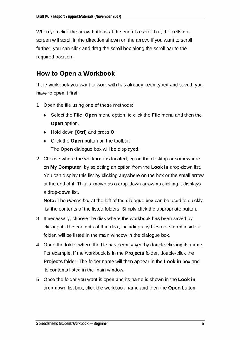
When you click the arrow buttons at the end of a scroll bar, the cells on-
screen will scroll in the direction shown on the arrow. If you want to scroll
further, you can click and drag the scroll box along the scroll bar to the
required position.
How to Open a Workbook If the workbook you want to work with has already been typed and saved, you
have to open it first.
1 Open the file using one of these methods:
♦ Select the File, Open menu option, ie click the File menu and then the
Open option.
♦ Hold down [Ctrl] and press O.
♦ Click the Open button on the toolbar.
The Open dialogue box will be displayed.
2 Choose where the workbook is located, eg on the desktop or somewhere
on My Computer, by selecting an option from the Look in drop-down list.
You can display this list by clicking anywhere on the box or the small arrow
at the end of it. This is known as a drop-down arrow as clicking it displays
a drop-down list.
Note: The Places bar at the left of the dialogue box can be used to quickly
list the contents of the listed folders. Simply click the appropriate button.
3 If necessary, choose the disk where the workbook has been saved by
clicking it. The contents of that disk, including any files not stored inside a
folder, will be listed in the main window in the dialogue box.
4 Open the folder where the file has been saved by double-clicking its name.
For example, if the workbook is in the Projects folder, double-click the
Projects folder. The folder name will then appear in the Look in box and
its contents listed in the main window.
5 Once the folder you want is open and its name is shown in the Look in
drop-down list box, click the workbook name and then the Open button.
Spreadsheets Student Workbook — Beginner 5

Draft PC Passport Support Materials (November 2007)
How to Save a Workbook When saving files to your computer, you can choose to save them in a folder
on your computer’s local hard disk, floppy disk or memory stick. If you are
attached to a network, you can also choose to save them in a folder on the
network. You can also choose to store it in a folder that already exists, or
create a new folder for it.
1 Choose to save the file using one of these methods:
♦ Select the File, Save menu option, ie click the File menu and then the
Save option.
♦ Hold down [Ctrl] and press S.
♦ Click the Save button on the toolbar.
The Save As dialogue box will be displayed.
2 In the File name text box enter a suitable file name. The following rules
apply when naming files:
♦ File names can be a maximum of 255 characters.
♦ Some characters cannot be used in file names. These include:
\ / * ? : ; " | < >
♦ Within a single folder each file name must be unique.
Microsoft Excel adds an .xls extension to all workbook file names. It may be
the case, however, that you do not see the file extension as its display
depends on how your system has been set up.
3 If necessary, choose the file format from the Save as type drop-down list.
4 Specify where the file is to be saved, eg on the desktop or somewhere on
My Computer, by selecting an option from the Save in drop-down list.
You can display this list by clicking anywhere in the box or on the small
arrow at the end of it.
Note: The Places bar at the left of the dialogue box can be used to quickly
display the contents of the listed folders. Simply click the appropriate
button.
Spreadsheets Student Workbook — Beginner 6

Draft PC Passport Support Materials (November 2007)
5 If necessary, choose the disk where you want to save the file by clicking it.
The contents of that drive, including any files not stored inside a folder, will
be listed in the main window in the dialogue box.
6 Open the folder where the file is to be saved by double-clicking its name.
For example, to store the file in the Projects folder, double-click the
Projects folder. The Project folder name will then appear in the Save in
box and its contents listed in the main window.
If you want to create a subfolder inside the one shown in the Save in box,
click the New Folder button. A new folder will appear in the file and folders
list, ready for you to type a unique name. Type the new folder name then
press [Enter].
7 Once the folder you want is open and displayed in the Save in drop-down
list box, click the Save button.
Note: When you save a file that has been saved before, Excel assumes that
you want to save it on top of the previous version and so doesn’t ask you for a
file name or a location. If you want to save another copy of the file, use the
File, Save As menu option, which will always ask you for a file name and a
location.
Printing a Workbook To print a copy of your workbook to the default printer, click the Print button
on the toolbar. The worksheet can be printed using standard layouts like
portrait or landscape (useful for spreadsheets that need to display across the
page, rather than down the page). It may be necessary to adjust the page
orientation (portrait or landscape) or even adjust the margins, size of font
and/or page sizes to get your worksheet to fit onto one page. There are a
number or printer properties and page setup properties you can change to
allow your spreadsheet to look better, or to minimise paper.
Closing a Workbook When you have finished working with a workbook, you can close it using the
Close option from the File menu.
Spreadsheets Student Workbook — Beginner 7

Draft PC Passport Support Materials (November 2007)
Inserting, Deleting, Moving and Renaming Worksheets Each workbook that is created has one or more worksheets. The precise
number will depend on each system’s setup, however, you will be presented
with three worksheets by default.
You can add and remove worksheets as and when you need to and, as
you’ve seen earlier, you can also rename sheets to make them easier to work
with. If necessary, you can also change the order in which the sheets appear
in the workbook.
How to Insert a Worksheet into a Workbook 1 Right-click a worksheet tab.
2 Choose Insert from this menu.
3 In the Insert box, choose Worksheet and click OK.
The new sheet is inserted to the left of the one you right-clicked.
How to Move a Worksheet Click the tab of the worksheet that’s to be moved then drag it to its new
position in the workbook. As you drag, a small arrow shows you where the
worksheet will be placed if you let go of the mouse button.
How to Delete a Worksheet from a Workbook Right-click the tab of the worksheet you want to delete and choose Delete
from the shortcut menu. When you’re asked to confirm the deletion, click OK.
How to Rename a Worksheet Double-click the worksheet tab and type the new name for the sheet. Press
[Enter] when you’ve finished.
Common Spreadsheet File Formats When you save an Excel workbook it is stored in a particular format, complete
with the cell contents, the formatting that has been applied, the graphics that
have been included and so on. The file name you supply is given an .xls
extension (an abbreviation added to the end of the file name to identify the file
type) which identifies it to Excel as an Excel workbook.
Spreadsheets Student Workbook — Beginner 8

Draft PC Passport Support Materials (November 2007)
Excel can both read and save your workbooks in other formats. This is so that
you can exchange data with other programs that can’t read or create Excel’s
own format. So if, for example, a client uses a different spreadsheet program
that can’t read Excel files, you could save the workbook in another format that
they can read. Likewise, if Excel can’t read their spreadsheet program’s file
format, they could save their workbook in one of the formats that Excel can
read.
Text files When you save a workbook using one of the text formats, only the text and results of calculations are saved. This means that you lose all formatting, graphics, objects and other contents from the file. Normally you would use the Text (Tab-delimited) (*.txt) file type. When you use this type, the resulting file contains all the text with each row from the worksheet shown on a new line, and with tab characters between the columns. Files of this type have a .txt extension on their names. Note: If you’re saving a text file for a Macintosh computer user, use the Text (Macintosh) (*.txt) file type.
Comma Separated Value (CSV) files
This format also saves text and results of calculations, with the rows on separate lines of the CSV file and the columns separated with commas. Files that use this format can be identified by their .csv file name extension. Note: If you’re saving a CSV file for a Macintosh computer user, use the CSV (Macintosh) (*.csv) file type.
Symbolic Link (SYLK) files
When you save a workbook using the SYLK format, the text and the formulas (used to perform the calculations) are saved along with limited formatting. If any part of a formula is not supported by the SYLK format, the result of the calculation, rather than the formula used to calculate it, will be saved in the SYLK file. Files that use this format can be identified by their .slk file name extension.
To open or save a workbook in a format other than the standard Excel
Workbook format, use the Files of type drop-down list to choose the
particular format you want to work with.
Using Excel Help Like all Microsoft applications, Excel provides an online facility for getting help
when you need it.
Spreadsheets Student Workbook — Beginner 9

Draft PC Passport Support Materials (November 2007)
The Office Assistant The Office Assistant is an online help system that you can use when you want
to know more about a particular option or how to complete a task. If the Office
Assistant is displayed, some of the prompts that are usually shown in dialogue
boxes appear in an Office Assistant balloon.
1 Select the Help, Microsoft Excel Help menu option. Alternatively, click
the Office Assistant button at the end of the Standard toolbar, or press
the function key marked [F1]. An Office Assistant balloon will be displayed.
2 Type your question into this What would you like to do? box. For
example, How can I sort information? and then click the Search button.
You will then be given a choice of help topics to choose from.
3 Click your chosen topic and help text will be displayed or a list of headings
will be shown so you can select more specifically what you would like to
do.
4 Click your chosen heading to display the help text.
Creating Workbooks As you learned earlier, each workbook created in Excel is based on a
template that defines its initial appearance and layout. This means that the
fonts, sizes and so on give the workbook a consistent look and feel without
each user having to spend the time and effort creating the same effects.
There are a number of templates for different workbook types including
expense statements, invoices and purchase orders, and you can create your
own if necessary.
If you choose to create a new workbook using the New button on the toolbar,
it will be based on the default Normal template.
If you want to create a workbook based on one of the other templates, you
have to use the File, New menu option as this will give you a choice of
templates to choose from.
Spreadsheets Student Workbook — Beginner 10

Draft PC Passport Support Materials (November 2007)
This is an illustration of a workbook based on the Expense Statement template that’s supplied with Excel. As you can see, content and formatting
are part of the template. Once the workbook has been created, you simply fill
in the blanks with your figures. The Total and Sub Total cells contain
calculations (formulas) that will work out the figures based on what you typed
into the other cells.
Workbook Templates Templates allow you to create workbooks that already have the formatting you
need as well as standard text such as column or row labels, graphics such as
logos, or formulas for calculating the values needed to complete your
workbook.
Spreadsheets Student Workbook — Beginner 11

Draft PC Passport Support Materials (November 2007)
For example, if you had to complete a time sheet every week, it would be
quicker to set up the basic sheet as a template (complete with headings and
column and row labels, as well as the calculations needed to total your hours)
then every week create a workbook based on the template, simply filling in the
blanks with the relevant data for that week.
Every workbook you create is based on a template and unless you choose a
specific one, it will be based on the Normal template. This template doesn’t
add any standard content to your workbook, but applies a basic font and
number format to each cell. You will learn how to create a workbook from a
template later.
You can create templates yourself by creating what you need as an ordinary
workbook and then saving it as a template using the Template (*.xlt) option
from the File of type drop-down list in the Save As dialogue box. Templates
are recognised by their .xlt extensions.
How to Create a Workbook Using a Template 1 Select the File, New menu option.
2 Click the template you want to use then click OK.
A new workbook will be created based on the template you chose in the
dialogue box. This is the workbook that you’ll type your own data into. The
template stays the same so that you can use it again later.
Entering Numbers, Text and Symbols in a Cell Text, numbers, symbols, dates and times can simply be typed into a cell. Just
move the active cell pointer to the cell where the data is to appear and then
type it.
Note: You can move the active cell pointer to a cell either by clicking it using
the mouse or by using the arrow keys on the keyboard to move it from its
current location. Pressing [Ctrl] [Home] will move the pointer immediately to
cell A1.
Spreadsheets Student Workbook — Beginner 12

Draft PC Passport Support Materials (November 2007)
♦ To accept what you have typed, press the [Enter] or [Tab] key.
— If you press [Enter], the cell pointer will move down one row.
— If you press [Tab], it will move right one column.
♦ If you want to abandon what you have typed, press the [Esc] key.
When entering data you will notice that text entries are lined up at the left of
the cell, while numeric entries are lined up at the right. Text entries are
referred to as labels and numeric entries, dates and times are referred to as
values.
Note: A text entry that's too wide for the cell you've typed it into will spill over
into the cell to the right, as long as that cell’s empty. If there's something in the
next cell, you will only see as much of your text entry as fits in the cell without
spilling.
Editing Data To make changes to a cell, either double-click it or press [F2] on your
keyboard. You can then move around the entry, editing it to suit your needs.
Pressing the [Backspace] key will delete data to the left of the cursor that’s
shown in the cell when you edit it, and [Delete] will delete data to the right.
Alternatively, you can replace the entire cell contents simply by clicking the
cell and typing the new entry.
Using Undo Your most recent actions can be undone using the Undo drop-down list or the
Edit, Undo menu option. If you undo an action or list of actions then discover
that you shouldn't have, use the Redo drop-down list or the Edit, Redo
command.
Spreadsheets Student Workbook — Beginner 13

Draft PC Passport Support Materials (November 2007)
Entering Simple Formulas in a Cell When you want to perform a calculation using numbers stored in a
spreadsheet, you enter a formula. One of the main benefits of using a formula
that uses cell addresses, rather than doing the calculation yourself and simply
typing the answer into a cell, is that formulas are automatically updated when
any cell on the sheet is changed or a new entry is made. This means that you
can change the values that are used in the calculation without having to work
out the result again.
Example Formula
=6+7+2 If you type this formula into a cell, the result (15) will be
displayed in the cell. If you wanted to see the formula, you would
click the cell then look at the formula bar.
Formulas always start with an = (equals) sign so that Excel can identify them
as formulas. What follows the equals sign is the calculation that is to be
performed. Although the example above uses numbers, it is usually better to
use cell addresses so that the automatic updating of formulas is effective. For
example, if you want to add the contents of cells B3 and B4, the formula
would read =B3+B4. This means that if the contents of either of these cells is
changed, the result of the formula would be updated to match.
If you want to multiply the contents of cell B3 by B4, use the * (asterisk)
character. In this case the formula would read =B3*B4. Division uses the / (oblique) character. These characters used in this way are called operators.
Operators * Multiply
/ Divide
+ Add
- Subtract
% Per cent
^ Exponent (to the power of)
Spreadsheets Student Workbook — Beginner 14

Draft PC Passport Support Materials (November 2007)
Formula Construction To enter a formula into a cell, first place the active cell pointer on the cell
where the result is to be shown. Next, type = followed by the calculation you
want to perform. You can either type the addresses of the cells you want to
use or, once you have typed the = sign, you can click the cells, typing the
required operator between them.
BODMAS When you create a formula using more than one of the operators listed above,
Excel will perform the various parts in a specific order. This can mean you get
unexpected results. For example, what would you expect the result of this
formula to be?
=10+5*2
Did you guess 30? If so, you’d find that Excel got a different answer. The
answer that Excel would display would be 20. This is because of the order in
which the operators are carried out. BODMAS is a way or remembering this
order:
Brackets
Order (power of)
Division
Multiplication
Addition
Subtraction
Here’s another example along with an explanation of how Excel would deal
with it:
=5+60/5*(1+2)2-1
Brackets =5+60/5*(3)2-1
Order =5+60/5*9-1
Division =5+12*9-1
Spreadsheets Student Workbook — Beginner 15

Draft PC Passport Support Materials (November 2007)
Multiplication =5+108-1
Addition =113-1
Subtraction =112
The AutoFill Handle and Formulas The AutoFill handle is the small square at the bottom right corner of the
active cell pointer. This handle can be used to fill in series of entries and can
also be used to copy cell contents from one cell to other cells beside it. When
you copy a cell with a formula, the cell references in the formula are changed
to suit the cells they’ve been copied to.
The AutoSum Button The AutoSum button on the toolbar can be used to quickly add a row or
column of values. Simply place the active cell pointer on the cell where the
total is to be shown and then click the button. Excel will add the nearest set of
values. Press [Enter] to accept the suggested values.
Exercise 1: Using Copy and Cut
1 Make sure that Excel is open.
2 Open the workbook Clothes stored in your main folder.
3 Use the AutoSum button to complete this table.
4 Follow these steps to duplicate and move this table, adjusting the values
for Ladies’ Wear and Children’s Wear.
♦ Select the Men’s Wear table (A4:F11).
Spreadsheets Student Workbook — Beginner 16

Draft PC Passport Support Materials (November 2007)
♦ Click the Copy button on the Standard toolbar.
♦ The copy is to be placed beginning at cell A15, so click this cell then
click the Paste button on the Standard toolbar.
♦ Edit cell A15 to read Ladies’ Wear.
♦ Change some of the values in cells B17:E21, but be careful not to
change any of the totals — these values are calculated for you. Notice
that they change as you change the values in the rest of the Ladies’
Wear table.
♦ Make a copy of the Ladies’ Wear table, pasting it at cell A26.
♦ Edit cell A26 to read Children’s Wear and make some changes to the
values in the table.
The Ladies’ and Children’s Wear tables are to be moved onto separate
worksheets within the Clothes workbook.
♦ Select the Ladies’ Wear table (A15:F22) and click the Cut button on
the toolbar.
♦ Paste this table on Sheet 2 at cell A4 then change the column widths
as necessary.
Cut and paste the Children’s Wear table at cell A4 on Sheet 3 then change
the column widths as necessary.
♦ Copy and paste the headings in rows 1 and 2 on Sheet 1 for Sheet 2
and Sheet 3.
5 Rename each of the sheets by double-clicking its name, eg Sheet 1 at the
bottom of the worksheet and typing Men’s Wear, Ladies’ Wear and
Children’s Wear as appropriate.
6 Save the changes you’ve made to this workbook.
7 Close the workbook.
Spreadsheets Student Workbook — Beginner 17

Draft PC Passport Support Materials (November 2007)
Recognising Standard Formula Error Messages Until you are familiar with formulas, you might find that you make a few
mistakes. Most times, reading the message will explain what the problem is
and often Excel will suggest a way to fix it, sometimes even fixing it for you.
A less straightforward error is the circular reference. A circular reference is
caused when a formula includes the address of its own cell. For example, if
the formula =B6*B7 appears in cell B7, you will have created a circular
reference. Excel indicates this by displaying a message on the status bar and,
depending on how you created the formula, a dialogue box may appear giving
further details of your error.
Note: If the Office Assistant is switched on, this message will look different but
will contain the same information.
To resolve the problem, edit the formula to remove or correct the problem.
An Error That Isn’t an Error It’s common for users to think that they’ve made a mistake when the result of
a formula they’ve entered looks like this:
Jan Feb Mar Apr Total
North 700.12 35.86 367.81 467.01 #####
The problem here isn’t a mistake with the formula; it’s just that the column
isn’t wide enough to show the number. To fix it, just make the column wider.
Checking Your Calculations Although formulas will perform your calculations for you, you should always
check that you’re getting the result you expected. As BODMAS shows, you
might not get an error message, but that doesn’t mean that your formula is
giving you the result you want.
Spreadsheets Student Workbook — Beginner 18

Draft PC Passport Support Materials (November 2007)
Formula Calculation Each time you make a change to the data in your spreadsheet, all the
formulas dependent on the cell you’ve changed are recalculated so that they
can take account of the change. This is called automatic calculation and is the
default calculation mode.
Depending on how you work, you may prefer to switch the calculation mode to
manual, in which case each time you want to update the formulas affected by
the changes you’ve made, you would press the [F9] function key. To switch
the calculation mode to manual (or back to automatic), select the Tools, Options menu option and view the Calculation tab. Set the appropriate
option in this box then click OK to apply it.
Exercise 2: Using Copy and Paste
1 Open the workbook Dealer Pricing stored in the Cars folder in your
PersonalStuff folder.
This workbook contains a number of formulas to calculate values for the
first product PLA/001/46. These formulas are to be copied for the other
products in the list.
2 Follow these steps to copy the formulas and paste them for the other
products.
♦ Select the formulas in cells C6:H6.
♦ Make sure the mouse pointer is on the selected range then right-click
to display the shortcut menu.
♦ Click Copy on the shortcut menu.
Because these formulas are to be pasted for more than one product,
you have to select all the cells that will be filled with the copied
formulas.
♦ Select the range C7:H13.
♦ Point to the highlighted range then right-click and choose Paste from
the shortcut menu.
Spreadsheets Student Workbook — Beginner 19

Draft PC Passport Support Materials (November 2007)
♦ The formulas are repeated on each row and since they all contain
relative cell references, they are updated to match so that on each row
they calculate the figures for that row.
3 Add your name to the footer on this workbook then print one copy.
4 Save the changes you’ve made and close the workbook.
Selecting Cells, Range of Cells, Rows or Columns Before you can carry out an operation affecting a number of cells (a range),
you must identify the cells to be included in the range by selecting them. If the
operation is to affect only one cell, then simply click it to select it. To select
one or more ranges of cells you would use different methods, depending on
whether they’re together on the worksheet or not.
Selecting a Range of Adjacent Cells If you want to select a single range of cells that are side by side on the
worksheet, click the first of the cells then, holding down the left mouse button,
drag the mouse to the last. Alternatively, click the first of the cells and release
the mouse button. Then, holding down the [Shift] key, click the last cell. Both
these cells and all those in-between will be highlighted as selected.
Selecting Non-adjacent Cells and Ranges If the cells you want to select don’t appear side by side, you can select them
by clicking the first and then, holding down [Ctrl], clicking each of the others.
To select non-adjacent ranges, click and drag the first range and then, holding
down [Ctrl], click and drag the others.
Selecting a Single Row or Column To select a single row or column, click the grey button displaying the row
number or column letter.
Spreadsheets Student Workbook — Beginner 20

Draft PC Passport Support Materials (November 2007)
Selecting a Range of Rows or Columns To select a number of rows or columns that appear together on the sheet,
click and drag over the grey buttons indicating the row numbers or column
names.
To select multiple rows or columns that do not appear together in the sheet,
click and, if necessary, drag over the first set of rows or columns and then,
holding down [Ctrl], click and drag over the others.
Inserting and Deleting Rows or Columns To insert a new row, select the row it’s to be placed above and then choose
the Insert, Rows menu option. Alternatively, hold down the [Ctrl] key and
press the + key on the numeric keypad.
To insert a new column, select the column it’s to be placed before and then
choose the Insert, Columns menu option. Alternatively, hold down the [Ctrl] key and press the + key on the numeric keypad.
To delete rows or columns, first select them and then choose the Edit, Delete
menu option or press [Ctrl] — (on the numeric keypad).
Changing the Column Width If you need to change the column width to allow for long entries in a cell, you
can do so by clicking and dragging the vertical bar between the column
heading letters. Alternatively, point to this bar and double-click to make the
column wide enough so that the widest entry in that column is fully visible.
Using the AutoFill Handle to Enter Data Excel’s AutoFill feature can be used to quickly fill a range of cells with a series
of values, numbers or dates by use of the AutoFill handle, which is the small
square at the bottom right corner of the active cell pointer.
Spreadsheets Student Workbook — Beginner 21

Draft PC Passport Support Materials (November 2007)
To create a series, type the first entry in the series and then click and drag the
AutoFill handle to the right or down over the cells to be filled to complete the
series. As you drag, a Screen Tip will be displayed showing the entry that will
be filled in the current cell.
So, for example, if a series of months are to be entered into row 4, you would
type January into the first cell and then point to the AutoFill handle and drag it
to fill in the months you need. You can see the tip that’s displayed to show
you what month will be filled in the cell you’re at.
Formatting Cells The format of a cell containing a number dictates how it is shown in that cell.
For example, if you type the number 10 into a cell, it will, by default, be shown
as you’ve typed it. If you then format that cell as a percentage, the value in the
cell will be shown as 100%; if you format it as a currency it will be shown as
£10.00 (unless you also change the number of decimal places).
Note: You can quickly format a cell by typing the value the way you want it
displayed. If, for example, you type £10 into a cell, it will be formatted as
currency with no decimal places. Any value you type into this cell will now be
shown in this format unless you type it in another format.
The Format, Cells menu option and, for some formatting options, the
Formatting toolbar can be used to change the way values appear in the
selected cells.
Formatting Plain Numbers Plain numbers can be formatted to increase or decrease the number of
decimal places displayed and also to include a comma to separate hundreds
and thousands. These options can be adjusted using the Formatting toolbar.
First select the cells to be affected by the change, then click the appropriate
button.
Formatting Dates Dates can be formatted in a number of ways to suit the sheet you’re working
on. The Format, Cells menu option gives you access to the available formats.
Spreadsheets Student Workbook — Beginner 22

Draft PC Passport Support Materials (November 2007)
Formatting Currencies A quick way of formatting a value with your default currency format is to use
the Formatting toolbar. You can also use this toolbar to adjust the number of
decimal places shown.
Simply select the cell or range you want to format and then click the
appropriate buttons.
Alternatively, you can choose from a number of different currency symbols
using the Format, Cells command.
Formatting Percentages When you format a cell as a percentage, the value in the cell is multiplied by
100 and a % symbol is displayed. You can use the Formatting toolbar to do
this.
Formatting Text To allow you to highlight specific parts of your worksheets, the format of
letters and numbers within a cell can also be changed, for instance, by
changing the font style, colour or size. The Formatting toolbar contains a
number of buttons that can be used to make these changes to the selected
cells.
In addition to these formatting options, you can change the orientation of the
entries in the selected cells. To do this you would use the Format, Cells
command, clicking the Alignment tab.
Aligning Cell Contents When you first enter text into a cell, it is aligned to the left of the cell, whereas
numeric values including plain numbers and dates are aligned to the right.
This horizontal alignment can be changed using the Formatting toolbar or the
Format, Cells command which gives you additional options. Another
horizontal alignment option that is available is the Merge and Centre option
which lets you treat a number of cells as one and centre the contents within
the one new cell.
Spreadsheets Student Workbook — Beginner 23

Draft PC Passport Support Materials (November 2007)
You can also change the vertical alignment of a cell, ie align the entry to the
top, centre or bottom of a cell that is deeper than the entry.
Adding Cell Borders Using cell borders allows you to highlight ranges of cells within your
worksheets. You can add preset borders to the selected range using the
Borders drop-down list on the Formatting toolbar or customise the borders
using the Format, Cells menu option.
Using the Format, Cells menu option you can set your own choice of borders
for the range of cells that is currently selected. In the Border tab, you can
choose one of the preset borders or choose a style and colour and then apply
it to the required border.
Copying Cell Formatting You can quickly copy all the formatting attributes that have been applied to
one cell and apply them to another cell or a range of cells.
First click the cell that’s been formatted with the attributes you want to copy
and then click the Format Painter button on the toolbar.
Next click the cell that’s to be formatted with these attributes. Alternatively, to
apply these same attributes to a range of cells, click and drag over the cells.
Note: If you want to apply the attributes to more than one cell or range of
cells, double-click the Format Painter. When you’ve finished copying the
formatting, click it again to switch it off.
Formatting Other Numbers The Format Cells box can be used to apply any number format you want to
use. On the Number tab (shown under Formatting Currencies box above)
you can choose any of the formatting categories and set the specific options
for each. Clicking OK will apply your settings to the selected cells.
Spreadsheets Student Workbook — Beginner 24

Draft PC Passport Support Materials (November 2007)
Using AutoFormat The AutoFormat feature in Excel can be used to add a collection of formatting
attributes to your data in one step. There are a number of different
AutoFormats to choose from and even if none of them is exactly what you
want, you can adapt it to suit yourself. The Format, AutoFormat menu option
gives you the list of AutoFormat to choose from.
Conditional Formatting When you want to highlight cells that match specific conditions, you can do so
by applying formatting attributes via the conditional formatting feature. For
example, you might want to emphasise cells that fall outside limits that you’ve
specified. By using a different font, style, pattern and/or border, you can draw
attention to these cells.
How to Apply Conditional Formatting 1 Select the cells to be formatted.
2 Select the Format, Conditional Formatting menu option.
3 Make the appropriate selections:
♦ To format value cells based on their contents:
a) Select Cell Value Is from the Condition 1 drop-down list.
b) Next, select a comparison from the Comparison drop-down list. The
entries in this list include equal to; not equal to; greater than; less than and between.
c) Enter the values required for the comparison you've chosen into the
text box. These values can be numbers or formulas.
♦ To format cells based on a condition other than their values:
a) Select Formula Is from the Condition 1 drop-down list.
b) Enter the required formula into the text box. This formula will include
references to the relevant cells in the first row in the selected range.
The result of the formula must be either True or False.
4 Click the Format button.
Specify the formatting attributes you want to apply to those cells that
match the specified condition. When you’re finished, click OK to return to
the Conditional Formatting dialogue box.
Spreadsheets Student Workbook — Beginner 25

Draft PC Passport Support Materials (November 2007)
5 If you want to set other conditions, click the Add button then repeat steps
3 and 4 for up to two others.
6 When you've set all the required conditions, click OK to apply them to the
selected cells.
Exercise 3: Cell Formatting and Calculations
1 Create a new blank workbook and create the following table:
Note: Type the £ sign as part of the monthly salaries but not the comma
— Excel will format the number this way.
2 In cell C4 enter a formula that will calculate Anne Gilchrist’s annual salary
as 12 times her monthly salary.
This formula should read =B4*12
3 In cell D4 calculate Anne’s annual bonus as 10% of her annual salary
This formula should read =C4*10%
4 Copy these formulas and paste them for the other employees.
5 Select cells B12:D12 then use the AutoSum button to give totals for these
columns.
6 Andy’s last name has been entered incorrectly. Edit this cell to read Andy Garden.
7 Nicola’s monthly salary is wrong: it should be 1990. Make this edit and
notice that the annual salary and bonus are recalculated to reflect this
change. The totals on row 12 are also updated.
Spreadsheets Student Workbook — Beginner 26

Draft PC Passport Support Materials (November 2007)
8 Change the worksheet name to Sales Dept by double-clicking the Sheet 1
tab and typing the new name.
9 Copy all the information from the Sales Dept sheet and paste it on Sheet 2.
10 Rename this sheet Admin Dept.
11 Change the information in columns A and B only as shown below (all cells
with formulas will be updated automatically).
12 Admin department staff receive a 7.5% bonus rather than 10%, so change
the column label in cell D3 and then the formula in cell D4 to reflect this.
13 Copy the formula for all other staff in the Admin department.
14 Follow these steps to print one copy of both worksheets:
♦ Add your name to the footer.
♦ Select the File, Print menu option.
♦ Under Print what, click Entire workbook.
♦ Click OK.
15 Save the workbook as Bonus Sheet in the Financial folder in your
WorkStuff folder, then close it.
Exercise 4: Using Formulas
1 Open the workbook Salary Rises stored in the Financial folder in your
WorkStuff folder.
Spreadsheets Student Workbook — Beginner 27

Draft PC Passport Support Materials (November 2007)
2 Enter a formula into cell C6 that will calculate the annual salary of Paul Hull by multiplying his monthly salary by 12, then copy the formula for the
other employees.
3 Cell B3 contains the percentage rise that the employees are to be given.
This percentage is in a separate cell to make it easier to change if
necessary. If the percentage was included as part of each formula, you
would have to change every formula if the percentage changed. By putting
the percentage in its own cell and then including a reference to that cell in
the formulas, you would only have to change one cell if the percentage
changed.
Follow the instructions below to enter a formula that will calculate the
increase for Paul Hull into cell D6 and then copy it for the other
employees.
♦ Position the cell pointer on cell D6 then type =C6*B3
♦ Copy this formula for the other employees and look at the results.
♦ The results of these pasted formulas are clearly not correct, so click
cell D7 and look at the formula bar.
The formula in this cell reads =C7*B4 since it uses relative cell
addressing. However, B4 is an empty cell. The formula should be
multiplying Stephen’s annual salary (C7) by the increase percentage
(B3), so the original formula needs to include absolute markers to make
sure that B3 doesn’t change when the formula is copied.
♦ Move to C6 and type the formula =C6*$B$3 (you can type the $
symbols, or press the F4 function key when the cursor is next to the B3
address).
When this formula is copied now, C6 will change but B3 won’t.
♦ Copy this formula for the other employees. This will overwrite the
original incorrect formulas.
♦ Click cell D10 and look at the formula in the formula bar. The reference
to cell C6 has been changed to reflect the formula's new row, but the
reference to cell B3 remains the same.
4 Enter a formula into cell E6 that will calculate Paul Hull’s New Salary
(annual salary + increase) then copy it for the other employees.
Spreadsheets Student Workbook — Beginner 28
Draft PC Passport Support Materials (November 2007)
5 Calculate the totals on row 11 for each of the columns.
6 Notice the total increase shown in cell D11. The management have
budgeted to spend a maximum of £6,200.00 on salary increases and, as
you can see, awarding a 5% increase will exceed the budget. As the
increase percentage is being taken from cell B3, type other values, such
as 3.5% and 4.25%, into cell B3, to find the highest percentage that
management could award without exceeding its budget.
7 Save the changes to the workbook and then close it.
Exercise 5: Using AutoSum and Other Formatting Options 1 Open the P&L workbook stored in the Financial folder in your WorkStuff
folder.
2 Use the AutoSum button to enter totals in the ranges D5:D7, B8:D8, D11:D32 and B34:D34.
3 Follow the instructions below to replace all occurrences of the word
Revenues with the word Sales.
♦ Move the cell pointer to cell A1 and then choose the Edit, Replace
menu option.
♦ In the Replace dialogue box in the Find What box type Revenues. In
the Replace with box, type the word Sales.
♦ Select the Find Next button. The first cell containing the word
Revenues is highlighted.
Notice that this isn’t the only word in the cell, so if you’d ticked Find entire cells only, this occurrence of Revenues would not have been
highlighted.
♦ Click the Replace button. Excel now highlights the next occurrence.
♦ Click Replace. This occurrence is replaced and the cell pointer stays
on this cell, indicating that there are no more occurrences of the word
Revenues.
Spreadsheets Student Workbook — Beginner 29

Draft PC Passport Support Materials (November 2007)
♦ Notice that, although cell A7 also contains the word revenues, Excel
doesn’t move on to this occurrence. This is because it doesn’t have a
capital ‘R’.
4 Use Replace to replace all occurrences of the word Wages with Salaries.
5 Use Replace All to replace all occurrences of the word costs with fees.
Notice that when you use the Replace All button instead of the Replace
button you don’t see the individual occurrences before they’re replaced.
You should be careful when using this feature.
6 Save the changes you’ve made and close the workbook.
Copying, Moving and Deleting
How to Use Copy and Paste The Copy and Paste options available from either the toolbar or the Edit menu can be used to duplicate cell contents in another part of the worksheet
or in another open workbook altogether.
1 Select the cell(s) whose contents are to be duplicated elsewhere.
2 Click the Copy button or select the Edit, Copy menu option.
3 Display the sheet where the copied cell(s) is to be put and then position
the active cell pointer at the top left of the range where it is to be placed.
This can be in the same sheet, the same workbook or in another open
workbook altogether.
4 Click the Paste button or select the Edit, Paste menu option.
Note: The AutoFill handle can also be used to copy cell contents to adjacent
cells.
How to Use Cut and Paste The Cut and Paste options available from either the toolbar or the Edit menu
can be used to move cell contents to another part of the worksheet or to
another open workbook altogether.
1 Select the cell(s) whose contents are to be moved.
2 Click the Cut button or select the Edit, Cut menu option.
Spreadsheets Student Workbook — Beginner 30

Draft PC Passport Support Materials (November 2007)
3 Display the sheet where the cut cell(s) is to be put and then position the
active cell pointer at the top left of the range where it is to be placed. This
can be in the same sheet, the same workbook or in another open
workbook altogether.
4 Click the Paste button or select the Edit, Paste menu option.
Using Drag-and-drop Another method of copying or moving cell contents is the drag-and-drop
method.
First select the cell or range of cells to be copied or moved, then move the
mouse pointer onto one of the edges of the highlighted range, away from the
AutoFill handle. When the mouse pointer changes to an arrow, click and drag
the selected range to its new position. This will move the range to a new
location. If you want to copy the selected cells using this method, hold down
the [Ctrl] key as you drag, releasing the mouse button before the [Ctrl] key
when you’ve finished.
Deleting Cell Contents You can remove the contents from a cell or cell range by first selecting the
required cell(s) and then pressing [Delete] on your keyboard.
Cell Referencing One of the real strengths of spreadsheets is their ability to harness the power
of formulas. In fact, you might say that formulas were the reason
spreadsheets were developed.
The keys to effective use of formulas in Excel are its built-in functions. Functions handle complex calculations automatically for the spreadsheet
designer. But in order to use functions or formulas, you must understand and
know how Excel handles cell references.
Cell References A cell reference tells Excel where the data it needs for a calculation is located. There are three ways to make a cell reference in an Excel formula.
Spreadsheets Student Workbook — Beginner 31

Draft PC Passport Support Materials (November 2007)
Most of the time Excel formulas use relative cell references. Relative cell
references are made up of the column letter and the row number. For
example, B3 is a relative reference for the cell located in the second column
from the left edge of the spreadsheet, on the third row. Columns are lettered
from left to right, starting with A. Rows are numbered from the top down,
starting with 1
We say that B3 is a relative reference because the cell’s location is ‘relative’
to any cell containing a formula that uses the contents of that cell. A relative
reference will update itself when the formula it is in is moved to another cell.
To make this a little clearer, suppose you created a formula in cell G3 to add
the values in all the cells in the third row between the third and the sixth
columns. The instructions to Excel would look like this in part:
(C3+D3+E3+F3).
To place this formula in cell G3, you would select cell G3 by clicking in it. You
would tell Excel that the expression in this cell is a formula. Do this by typing
an equal sign (=) into the cell or into the Formula bar at the top of the
spreadsheet. You would then enter the formula by typing it into the cell or the
Formula bar.
On the next row down, suppose you also want to total the cells in columns C
through F. Rather than retype the whole formula, just select G3, select Copy
from the Edit menu, and then select G4. Open the Edit menu and select
Paste.
When you copy the formula from cell G3 to cell G4, Excel automatically
adjusts the relative references to correct for being a row lower down. In cell
G4, the instructions to Excel will update to (C4+D4+E4+F4) without any
further work on your part.
However, sometimes you will want to have the cell references stay the same
when the formula is copied. For example, suppose you have a worksheet in
which you will total the daily cost of one of the raw materials used to produce
materials during a one-month period. It would be faster to set up the
worksheet if you didn’t need to enter the unit cost 30 times.
Spreadsheets Student Workbook — Beginner 32

Draft PC Passport Support Materials (November 2007)
It is much simpler to have constants in only one place and copy the formulas
from cell to cell. You can do this and still have everything come out right if you
use either absolute or mixed cell references.
An absolute cell reference does not change when a formula is copied from one cell to another. In a mixed cell reference, either the row or the column in the reference is made absolute, and the other part is relative.
Absolute cell references are created by placing dollar signs in front of the
column letter and row number. For example, $B$3 is an absolute reference to
the cell in the second column of the third row on a given worksheet. This
reference will always point to that cell, even if the formula containing the
reference is copied or moved to another cell.
However, $B3 is a mixed reference: B is absolute, 3 is relative. It will always
point to the same column when the formula it is in is moved or copied to
another cell, but the row will update.
Although cell references are designated as relative, absolute or mixed at the
time they are created, they can be easily changed to another type at any time.
To cycle between relative, absolute and mixed cell references, place the
insertion point within a cell reference in the Formula bar (not in front of the
equal sign) and then press the F4 key repeatedly until you get the reference
format you require.
To prevent cells with formulas being accidentally changed you could lock the
cell contents on the Protection tab of the Format Cells dialogue box.
Spreadsheets Student Workbook — Beginner 33

Draft PC Passport Support Materials (November 2007)
Exercise 6: Absolute/Relative Cell Referencing
Answer the following questions:
True or False?
By default, all cell addresses are Relative
The keyboard shortcut used to change F4 to
$F$4 in a formula is
Shift [F4]
$B7 in a formula in C7 copied to cells C8:C10 will
become
B8:B10
A$9 in a formula in F9, copied to cells G9:I9
becomes
B$9:D$9
Exercise 7: Absolute/Relative Cell Addressing and Statistical Functions Enter the following data into a new worksheet, using the following guidelines:
♦ Cell range C6:C9 — formulas
♦ Cell range D6:D9 — formulas
♦ Cell range C11:C15 — functions
♦ Format all figures appropriately (currency, percentage, integer, etc)
Spreadsheets Student Workbook — Beginner 34

Draft PC Passport Support Materials (November 2007)
1 Enhance the layout by formatting as required.
2 Use an appropriate function to display today’s date in D2.
3 Rename the worksheet Furniture Sale.
4 Put your name and today’s date in the worksheet footer.
5 Save your worksheet.
6 Take a printout showing formulas, with column and row headings and
gridlines displayed (adjust column widths to display complete formula if
necessary).
7 Take a printout showing data.
Formatting Text Formatting allows you to change the appearance of your spreadsheet,
perhaps to emphasise particular parts of it, or perhaps to make it look better.
Text Formatting Text formatting is formatting that affects the text itself, eg bold text, italic text,
font, font size (also known as point size) or font colour.
Some of these effects can be added using the toolbars, while all of them can
be added using the Format, Cells, Font menu option.
Spreadsheets Student Workbook — Beginner 35

Draft PC Passport Support Materials (November 2007)
Formatting Toolbar To apply formatting effects using the toolbar, first select the text you want to
apply the effect to and then choose the effect. For bold, italic and underline,
simply click the appropriate button to switch it on or off. For the other effects,
choose the option you want from the drop-down lists.
Superscript and Subscript If you want to display text or numbers in smaller than normal text and slightly
above or below it (eg in a mathematical expression) you can make use of
superscript or subscript. You can turn this off or on from within the Format Font menu option. Notice that it’s a check box under font effects and you will
see a preview of what the text would look like applying an effect in the preview
pane.
To display a smaller raised number after a letter you would use superscript,
eg P3.
Subscript — the opposite of superscript — allows you to place the number
lower than normal text, eg P3.
Remember whenever you turn on a font effect it will remain until you turn it off
again. There are other types available like Shadow, Emboss etc.
Alignment There are four alignment options: left aligns text to the left margin; centre
alignment aligns text to both left and right margins, but does not justify the
text, so text can be uneven; right alignment justifies text to the right margin;
and fully aligned justifies the text so it is even on both sides.
Format, Font Menu Option To apply formatting effects using the Format, Font menu option, first select
the text you want to apply the effect to. Next select the menu option and
choose the effects you want to apply. Once you’ve chosen all the effects you
want, click OK to apply them to the selected text.
Spreadsheets Student Workbook — Beginner 36

Draft PC Passport Support Materials (November 2007)
How to Use Formatting Options To further enhance the appearance of your spreadsheet, you can add borders
and shading to parts of it. The Format cells menu option has a number of
tabs that will let you choose the number, alignment, border, font and pattern
for a single cell or a range of cells.
Adding a Header or Footer Headers and footers let you add information such as the creation date, page
numbers or file name to printed pages of your workbooks. To create a header
or footer, select the View, Header and Footer menu option then display the
Header/Footer tab. You can select one of the standard headers or footers
from the drop-down lists in this tab, or you can use the Custom Header/Custom Footer buttons to create your own. You can also select
Headers and Footers from the File, Page Setup option.
Exercise 8: Formatting Cells
1 Open the workbook Sales Q2 stored in the Sales folder in your WorkStuff folder.
2 Following the instructions below, format all the money values on the sheet
to show thousands separated by commas and with two decimal places.
Spreadsheets Student Workbook — Beginner 37
Draft PC Passport Support Materials (November 2007)
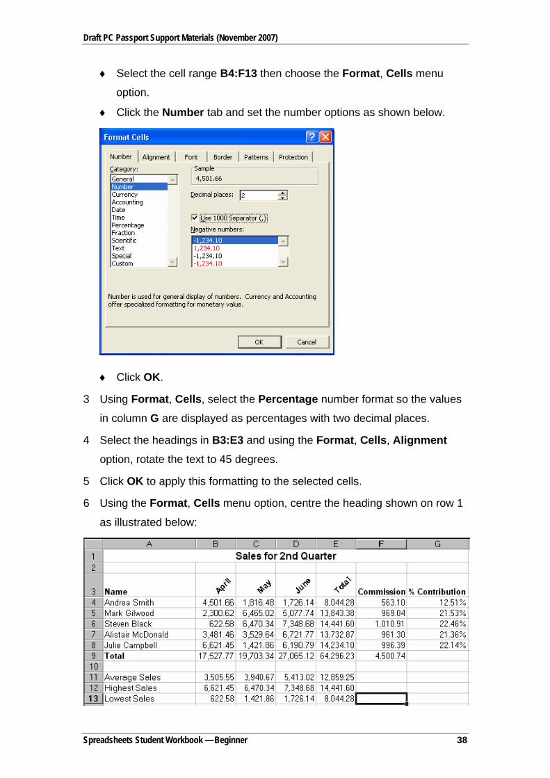
♦ Select the cell range B4:F13 then choose the Format, Cells menu
option.
♦ Click the Number tab and set the number options as shown below.
♦ Click OK.
3 Using Format, Cells, select the Percentage number format so the values
in column G are displayed as percentages with two decimal places.
4 Select the headings in B3:E3 and using the Format, Cells, Alignment option, rotate the text to 45 degrees.
5 Click OK to apply this formatting to the selected cells.
6 Using the Format, Cells menu option, centre the heading shown on row 1
as illustrated below:
Spreadsheets Student Workbook — Beginner 38

Draft PC Passport Support Materials (November 2007)
♦ Select A1:G1.
♦ Select Format, Cells and click the Alignment tab.
♦ From the Horizontal drop-down list choose Centre.
♦ Tick Merge cells and then click OK.
7 Practise using Format, Cells to apply the various formatting options
described below.
Cells A4:A8 Apply a left indent of 1
Cells B9:F9 Border: thin line top, double line bottom
Pattern: light grey background shading
Cells A11:E13 Border: thick blue line around range
Title Font: Times New Roman, 20 pt, Bold, Italic
8 Add your name to the footer, then print two copies of this workbook.
9 Save and close the worksheet.
Exercise 9: Using AutoFormat
1 Open the file called Sales Turnover held in the Sales folder in your
WorkStuff folder.
2 Follow the instructions below to use AutoFormat to change the
appearance of the worksheets.
♦ Select the range A1:E9.
♦ Select Format, AutoFormat and choose an AutoFormat layout.
♦ Click OK and the formatting will be applied to the selected range.
3 Try out one or two of the other AutoFormats until you find one you want to
use. Remember you can click the Options button to switch on or off
various elements of the AutoFormat.
4 Save and close the workbook.
Spreadsheets Student Workbook — Beginner 39

Draft PC Passport Support Materials (November 2007)
Previewing and Printing a Workbook Before printing data from a workbook, you can use Print Preview to check
how it’s going to look. When you choose the File, Print Preview menu option
you will see the document on the screen exactly as it will appear on paper. If
you need to make any last minute changes, you can do so within Print
Preview.
To begin, select the File, Print Preview menu option or click the Print Preview button on the toolbar.
If the preview looks okay, click the Print button on the toolbar to display the
Print dialogue box and make your selections to print the workbook. You can
learn about the Print dialogue box on the next page. You may feel that you
need to change the page orientation to landscape (sideways) to enable you to
get more of the spreadsheet onto one page. This is done in the printer’s
properties settings or if you’re in Print Preview from the Setup button.
If the spreadsheet prints over more than one page, you may want to adjust it
to ‘fit on one page’, however it will reduce the size of the font to accommodate
it fitting onto one page.
Note: When you return to the workbook after previewing it, a dotted line
shows you the right and bottom edges of each printed page.
Inserting Page Breaks Excel will insert page breaks when you choose to preview or print a
worksheet. When the worksheet is too long or too wide to fit on a page, any
extra rows and/or columns are moved onto a new page. Page breaks appear
as dotted lines on the worksheet.
However, if you decide that the page breaks should be positioned elsewhere,
you can insert a manual page break.
Spreadsheets Student Workbook — Beginner 40

Draft PC Passport Support Materials (November 2007)
To insert a manual page break, move the active cell pointer to the cell where
the break is to be inserted (the page break will be inserted above and to the
left of the active cell pointer), then select the Insert, Page Break command.
If you need to remove a page break, move the active cell pointer to the cell
where the break is and select the Insert, Remove Page Break menu option.
Using Page Break Preview Use the View, Page Break Preview menu option to see which cells will be
printed and where the page breaks are. Cells that will be printed are displayed
in white, while cells that are outwith the print range are displayed in grey. You
can change the page breaks by dragging them to a new location.
Printing To print a copy of the current (or active) sheet to the default printer, you
simply click the Print button on the toolbar.
If you want to print anything other than all the cells in the current sheet, eg
only part of the current sheet, more than one copy, or all the sheets in the
workbook, you would use the File, Print menu option.
How to Print in Excel 1 Select the File, Print menu option or press [Ctrl] P.
The Print dialogue box will be displayed
2 If the entire workbook is to be printed, continue and click on OK.
If only part of the worksheet is to be printed, select the required range(s).
If a specific worksheet in the workbook is to be printed in full, ensure that
the required worksheet is currently displayed.
Note: If more than one worksheet is to be printed in full, hold down the
[Ctrl] key and click each of the required worksheet tabs. The tabs will
appear highlighted.
3 Look in the Name box at the top of the dialogue box and ensure that the
correct printer has been selected. If not, click the Name drop-down button
to display the list of available printers, and select the correct printer.
Spreadsheets Student Workbook — Beginner 41

Draft PC Passport Support Materials (November 2007)
4 Make the required selections in the other groups in the dialogue box.
♦ Print range
All: Select the All option to print all pages.
Page(s): Select the Page(s) option and enter values into the From and
To text boxes to print a specific set of pages.
♦ Print what Selection: Select the Selection option to print the selected range of
cells.
Active sheet(s): Select the Active sheet(s) option to print the selected
range of sheets.
Entire workbook: Select the Entire workbook option to print the
entire workbook.
♦ Copies
Number of copies: Enter the number of copies required into the
Number of copies box.
Collate: Tick the Collate box to print one entire copy of the selection
before another copy is printed when you are printing multiple copies.
Note: If you want to see a preview of how the printed selection will look then
click the Preview button to display the Print Preview screen.
5 Click OK to start printing.
How to Print Part of a Worksheet 1 Select the cells to be printed.
2 Chose Print from the File menu and click on the Selection option.
3 Click OK.
How to Print Formulas If you want to print the calculation formulas rather than their results:
1 Select the Tools, Options menu option.
2 Select the View tab.
3 Under the Window options, tick the Formulas box.
4 Click on OK.
Spreadsheets Student Workbook — Beginner 42

Draft PC Passport Support Materials (November 2007)
When you return to your worksheet, the formulas will be shown in their cells.
Now when you print the worksheet, the formulas will be printed.
How to Centre the Worksheet A worksheet is printed to the left of the page and at the top. It is possible to
centre the sheet horizontally, vertically or both.
1 Select Page Setup from the File menu, or click on the Setup button in
Print Preview.
2 Click on the Margins tab.
3 In the Centre on page section (at the bottom), check either or both of the
Horizontal and Vertical boxes.
4 Click on OK.
How to Print Landscape The default print setting for your page orientation is portrait. Quite often, a
worksheet is wider than it is long and would be better printed in landscape.
1 Select Page Setup from the File menu, or click on the Setup button in
Print Preview.
2 Click on the Page tab at the top of the dialogue box.
3 In the Orientation section, check the Landscape option.
4 Click on OK.
How to Print the Worksheet Bigger or Smaller (Scaling) You may wish to make your worksheet bigger or smaller so that it fits better
on a single sheet, especially if parts of your spreadsheet run over onto
another page.
1 Select Page Setup from the File menu, or click on the Setup button in
Print Preview.
2 Click on the Page tab at the top of the dialogue box.
3 In the Scaling section, use the nudge buttons to change the Adjust to percentage.
4 Click on OK.
Spreadsheets Student Workbook — Beginner 43

Draft PC Passport Support Materials (November 2007)
How to Repeat Rows at the Top of Printouts 1 From the File menu, select Page Setup.
2 On the Sheet tab, click into the Rows to Repeat at top box.
3 Type in the row numbers you want to repeat (ie 1:1 for the first row or 1:2
for the first two rows) or drag on the required row numbers on the
worksheet behind the dialogue box.
4 Click on OK.
The rows should now appear at the top of every page.
How to Print Gridlines Gridlines are the dotted lines surrounding each cell.
1 If you have Print Preview displayed, click on the Setup button. Otherwise,
choose Page Setup from the File menu.
2 Click on the Sheet tab at the top of the box.
3 Click on the Gridlines option to check the box.
4 Click OK.
The gridlines within your data area should now be visible. For instructions on
adding your own borders see the section on How to Use Formatting Options.
How to Change Margins by Eye 1 Display the Print Preview.
2 Click on the Margins button at the top of the screen. Dotted lines appear
to show the current margin settings.
3 Drag on the dotted margin line until the required change is made.
How to Change Margins by a Specific Figure 1 Display your Page Setup box (either from the File menu or the Print
Preview screen).
2 Click on the Margins tab.
3 Type the specific figure you require in the appropriate margin box (or use
the nudge buttons).
4 Click on OK.
Spreadsheets Student Workbook — Beginner 44

Draft PC Passport Support Materials (November 2007)
Exercise 10: Printing Your Workbook
1 Open the workbook Production stored in your main folder.
2 View the document using the Print Preview button shown on the Standard
toolbar. You will see that the entire worksheet will be printed on a single
landscape page.
3 Close Print Preview.
4 Following the instructions below, insert a page break so that the
Production Analysis Across Both Plants information is printed on a
separate page.
♦ Move the active cell pointer to A18.
♦ Select the Insert, Page Break menu option. The page break is placed
above the cell pointer in cell A18.
♦ Select the View, Page Break Preview menu option so that you can
see the breaks more clearly.
♦ If the Welcome to Page Break Preview dialogue box is displayed,
click OK to close it.
♦ Move the mouse pointer onto the blue page break shown above row
18, then click and drag the page break up one row.
The page break has been moved to row 17.
5 Add your name to the footer of the workbook.
6 Click the Print Preview button on the Standard toolbar to see that rows 1
to 16 are printed on page 1. You can also see your name in the footer area
on this page.
Spreadsheets Student Workbook — Beginner 45

Draft PC Passport Support Materials (November 2007)
7 Click the Next button at the top of the preview window to see page 2,
which also contains the footer showing your name.
8 Follow these steps to print one copy of page 2 only.
♦ Click the Print button at the top of the preview window.
♦ Make sure the printer you want to use is shown in the Name box at the
top of the dialogue box.
♦ Make sure that Number of copies is 1.
♦ To print only page 2, enter 2 into the From box and the To box beside
Page(s) under Print range.
♦ Click OK to print your selection.
9 Select the View, Normal menu option to close Page Break Preview and
return to the normal view of your workbook.
10 Save the changes you’ve made and close the workbook.
Exercise 11: Working with Print Options
1 Open the file called Salary Increases held in the Financial folder in your
WorkStuff folder.
2 Follow the instructions below to preview your worksheet and use some of
Print Preview's features to alter its layout.
♦ Select the File, Print Preview menu option.
♦ Click once or twice on the Zoom button shown at the top of the Print Preview screen to increase and reduce the magnification of the
displayed page.
♦ If the margins are not shown, click the Margins button to display them.
♦ Increase the width of the Increase column by clicking and dragging the
column marker shown at the top of the Print Preview window to the
right.
♦ Click the Margins button again to hide the margins.
♦ Click the Setup button at the top of the preview window.
Spreadsheets Student Workbook — Beginner 46

Draft PC Passport Support Materials (November 2007)
♦ Display the Header/Footer settings. At the moment, the header is set
to display the name of the workbook centred within the header, and the
footer contains a centred page number.
♦ Click the Custom Header button.
♦ Click in the Centre section box after &[File] (which is a code for the
file name) and press [Enter] once to move the cursor to a new line.
♦ Click the Worksheet Tab button to add the sheet name to the header.
Click the Worksheet Tab button to add the worksheet name to the header.
♦ Click OK to return to the Header/Footer tab then click the Custom Footer button.
♦ Click the Date button to add the current date to the Left section box.
The Date button
♦ Add your name to the Right section box.
♦ Click OK and then OK again to return to the preview window.
The information you added to the header and footer is now shown on
the preview.
♦ Check the header and footer are as they should be, zooming in if
necessary to read the detail.
3 Follow these steps to print two copies of the workbook:
Spreadsheets Student Workbook — Beginner 47

Draft PC Passport Support Materials (November 2007)
♦ Click the Print button in the preview window.
♦ Enter 2 into the Number of copies box.
♦ Make sure that the printer you want to use is shown in the Name box
under Printer.
♦ Click OK to start printing.
4 Follow the steps below to display the formulas in the worksheet rather than
their results and then print them.
♦ Select the Tools, Options menu option and display the View settings.
♦ Under Window options, tick Formulas.
♦ Click OK to return to your workbook.
♦ Print one copy of the workbook.
♦ Select the Tools, Options menu option again and remove the tick from
Formulas.
♦ Click OK to return to the workbook.
5 Save and close the file.
Using Functions Functions are predefined formulas that let you carry out specific calculations.
For example, the SUM function allows you to add a range of cells without
defining them individually; the AVERAGE function allows you to find the
average of a range of values. The AutoSum button that you used earlier
inserts a SUM function into your worksheet. There are many functions
available in Excel; if necessary, you can find help on functions using the help
system.
All functions follow the same format:
=functionname(argument1, argument2, argument3…)
So, for example:
=SUM(B10:B20) This formula will calculate the total of all the values in the range shown.
=SUM(B10:B20, C10:C20) This formula will calculate the total of all the values in the ranges shown.
Spreadsheets Student Workbook — Beginner 48
Draft PC Passport Support Materials (November 2007)
=SUM(B10:B20,10,D19) This formula will calculate the total of all the values in the range shown plus 10 plus the value in cell D19.
=AVERAGE(B10:B20) This formula will calculate the average of all the values in the range shown.
=MIN(5,G7,H8) This will compare the value 5 and the values in cells G7 and H8, and will return the smallest value of the three.
=MAX(5,G7,H8) This will return the largest value.
Arguments are used to provide the function with data for its calculations. The
number and type of arguments needed will vary depending on the function. For example, the ROUND function, which rounds a given value to a specified
number of decimal places, has only two arguments (the value to be rounded
and the number of decimal places); while the SUM function has as many
arguments as necessary, up to the cell size limit. Some functions have no
arguments, however you must still include the brackets. An example of this
type of function is the TODAY function that returns the current date every time
the workbook is opened or printed. This would be typed in a cell as =TODAY()
If you type more than one argument, you must separate them using a comma
as shown in the examples above.
Using the SUM Function As previously mentioned, the SUM function is used to calculate the total value
of the contents of a range or ranges of cells. A range of cells is expressed by
naming the first cell in the range and the last cell in the range, separating the
two references with a : (colon). For example, A1:Z100 includes all the cells in
columns A to Z, rows 1 to 100. Therefore, the formula =SUM(A1:Z100) will
add together all the values in those cells and show the total in the cell
containing the formula.
The formula =SUM(A1:A10,C1:C10) will show the total of all the cell values in
the range A1:10 plus those in the range C1:C10.
Spreadsheets Student Workbook — Beginner 49

Draft PC Passport Support Materials (November 2007)
A SUM function can include values as arguments. In the formula
=SUM(A1:A10,10), 10 will be added to the total of the values in the cell range
A1:A10.
Using the AVERAGE Function The AVERAGE function is used to determine the average of a number of
values. Like the SUM function, it has an unlimited number of arguments. In
this example, =AVERAGE(A1:A10), the result will be the average of the
values held in those cells. Like the SUM function, the AVERAGE function can
include single cells, cell ranges, and values.
Using the MIN and MAX Function The MIN and MAX functions find the minimum and maximum values in a set
of values. Their syntax is =MIN(arguments) and =MAX(arguments). The
arguments may be cell references, constants, or a combination, for which you
want to find the smallest or largest value. Both of these functions ignore text,
blank cells (not zeros), error values, and logical values.
Spreadsheets Student Workbook — Beginner 50

Draft PC Passport Support Materials (November 2007)
Spreadsheets Student Workbook — Intermediate
Spreadsheets Student Workbook — Intermediate 51

Draft PC Passport Support Materials (November 2007)
Mathematical Functions
The SUM Function As previously mentioned, the SUM function is used to calculate the total value
of the contents of a range or ranges of cells. A range of cells is expressed by
naming the first cell in the range and the last cell in the range, separating the
two references with a : (colon). For example, A1:Z100 includes all the cells in
columns A to Z, rows 1 to 100. Therefore the formula =SUM(A1:Z100) will
add together all the values in those cells and show the total in the cell
containing the formula.
The formula =SUM(A1:A10,C1:C10) will show the total of all the cell values in
the range A1:10 plus those in the range C1:C10.
A SUM function can include values as arguments. In the formula
=SUM(A1:A10,10), 10 will be added to the total of the values in the cell range
A1:A10.
The ROUND Function The ROUND function rounds a given number to a specified number of
decimal places and so has only two arguments. For example, the formula
=ROUND(13.468,1) returns the result 13.5 by rounding 13.468 to 1 decimal
place. The number to be rounded argument can be a number or a cell
reference or a calculation, eg =ROUND(15.1254*2,2) returns the result 30.25.
Syntax =ROUND(number to be rounded, number of digits)
Spreadsheets Student Workbook — Intermediate 52

Draft PC Passport Support Materials (November 2007)
Statistical Functions
The AVERAGE Function The AVERAGE function is used to determine the average of a number of
values. Like the SUM function, it has an unlimited number of arguments. In
this example, =AVERAGE(A1:A10), the result will be the average of the
values held in those cells. Like the SUM function, the AVERAGE function can
include single cells, cell ranges, and values.
The MAX Function The MAX function returns the highest value from those provided as
arguments, and like the SUM and AVERAGE functions, the only limit to the
number of arguments is the cell limit.
=MAX(B10:B20) This formula will return the highest value out of those in the range shown.
=MAX(B10:B20,100) This formula will return the highest value out of those in the range shown or 100, whichever is highest.
The MIN Function The MIN function returns the lowest value from those provided as arguments,
and like the SUM and AVERAGE functions, the only limit to the number of
arguments is the cell limit.
=MIN(B10:B20) This formula will return the lowest value out of those in the range shown.
=MIN(B10:B20,100) This formula will return the lowest value out of those in the range shown or 100, whichever is lowest.
The COUNT Function The COUNT function counts the number of cells that have values in them in
the arguments you supply. In the example illustrated below, the COUNT
function is used to find how many cells in the range A1:A7 contain values
(rather than text entries).
Spreadsheets Student Workbook — Intermediate 53

Draft PC Passport Support Materials (November 2007)
The result of this formula is 3, as cells A2, A4 and A5 all contain values. A1,
A3, A6 and A7 contain non-numeric values, blanks or are empty, so they are
not counted.
=COUNT(B10:B20) This formula will return the number of cells containing values out of those in the range shown.
Note: The COUNTA function has the same syntax but returns the number of
cells containing any type of entry.
The COUNTIF Function The COUNTIF function will count the number of cells within a range that meet
the given criteria. For example, in the table below we could count the number
of cells that say apple, which would equal 3. COUNTIF will return numbers
only and works similar to DCOUNT, which is explained later.
Example Table
Spreadsheets Student Workbook — Intermediate 54

Draft PC Passport Support Materials (November 2007)
Syntax
COUNTIF(range,criteria)
♦ Range is the range of cells from which you want to count cells.
♦ Criteria are in the form of a number, expression or text that defines which
cells will be counted. For example, criteria can be expressed as ‘apple’.
Financial Functions
The PMT Function The PMT function is used to calculate the payments of a loan given the
amount of the loan, the interest rate per instalment period (eg monthly, yearly
or quarterly) and the number of instalments to be paid.
=PMT(4.25%/12,60,5000) This formula will return the amount of each monthly instalment on a loan of £5000 at 4.25% per annum over five years (60 months). Notice that the interest rate has been divided by 12 as the rate is an annual one but the payments are made monthly.
The full syntax of the PMT function is:
=PMT(interest rate per instalment period, number of instalments, amount of loan, future value of loan, type)
The future value of loan and type arguments are optional and so don’t have to
be supplied unless necessary. Future value of loan allows for an amount to be
outstanding at the end of the loan period while type allows you to specify
whether payments will be made at the start of each instalment period or at the
end. This can make a difference to the amount of interest that you would pay
and therefore to the payments.
Date and Time Functions Date and Time functions allow you to manipulate and display dates and times
within your spreadsheet. Excel calculates dates as numbers, so when you
specify a date, it is handled like this:
DATE(year, month, day)
Spreadsheets Student Workbook — Intermediate 55

Draft PC Passport Support Materials (November 2007)
Year The year argument can be one to four digits. Microsoft Excel interprets
the year argument according to the date system you are using. By default,
Excel in Windows uses the 1900 date system; Excel for the Macintosh uses
the 1904 date system.
Windows PC 1900 system
♦ If year is between 0 (zero) and 1899 (inclusive), Excel adds that value to
1900 to calculate the year. For example, DATE(108,1,2) returns January
2, 2008 (1900 + 108).
♦ If year is between 1900 and 9999 (inclusive), Excel uses that value as the
year. For example, DATE(2008,1,2) returns January 2, 2008.
♦ If year is less than 0 or is 10,000 or greater, Excel returns the #NUM! error
value.
Apple Macintosh 1904 System
♦ If year is between 4 and 1899 (inclusive), Excel adds that value to 1900 to
calculate the year. For example, DATE(108,1,2) returns January 2, 2008
(1900 + 108).
♦ If year is between 1904 and 9999 (inclusive), Excel uses that value as the
year. For example, DATE(2008,1,2) returns January 2, 2008.
♦ If year is less than 4 or is 10,000 or greater, or if year is between 1900 and
1903 (inclusive), Excel returns the #NUM! error value.
Month is a number representing the month of the year. If month is greater
than 12, month adds that number of months to the first month in the year
specified. For example, DATE(2008,14,2) returns the serial number
representing February 2, 2009.
Day is a number representing the day of the month. If day is greater than the
number of days in the month specified, day adds that number of days to the
first day in the month. For example, DATE(2008,1,35) returns the serial
number representing February 4, 2008.
Excel stores dates as sequential serial numbers so they can be used in
calculations. By default, January 1, 1900 is serial number 1, and January 1,
2008 is serial number 39448 because it is 39,448 days after January 1, 1900.
Spreadsheets Student Workbook — Intermediate 56

Draft PC Passport Support Materials (November 2007)
The DATE function is most useful in formulas where year, month,and day are
formulas, not constants.
DATEVALUE converts a date in the form of text to a serial number, eg
=DATEVALUE("23/7/2004")
NOW returns the serial number of the current date and time, eg =NOW()
TIME returns the serial number of a particular time, eg
=Time(Hour,Minute,Second)
TODAY returns the current date and needs no arguments, unlike some of the
other date and time functions, eg =TODAY()
These are the most common types of date and time functions and are a small
selection of the different types of functions you can get for dates and times.
Some will require values to be entered, and some will convert the differences
between two dates. Access the help files to experiment with these and others
you might find.
Logical Functions
The IF Function The IF function can be used to check whether a specific condition is true or
not, returning one result if the condition is true, and another if it's false.
Suppose you want to pay a £50 bonus to all sales staff who have exceeded
their £10,000 target. To do this you would check the total sales figures to see
who qualifies. If a sales representative’s total sales figure is greater than
£10,000, the bonus would be paid. Otherwise, the sales representative
doesn’t qualify for the bonus.
An illustration of this example follows.
Spreadsheets Student Workbook — Intermediate 57

Draft PC Passport Support Materials (November 2007)
Look at the formula that has been entered into cell C4. The formula is
constructed as follows:
=IF(B4>10000, 50, 0)
The results for the example are illustrated below.
Text Results
Should you want to display text as one or both of the results, you would
simply type the text enclosed in " (quotation marks) into the formula like this:
=IF(B4>10000, "Yes", "No")
In this example, the word Yes would be displayed for each sales
representative who qualifies for a bonus, and the word No for each sales
representative that doesn’t.
You can nest IF statements within each other. For example, say you want to
grade student assessments from A to F. If you had the values listed from 40–
99, you could say if value >40 and <45, Grade F. Notice the IF statement
uses some of the other conditional operators.
Spreadsheets Student Workbook — Intermediate 58

Draft PC Passport Support Materials (November 2007)
Conditional Operators The previous example uses the > (greater than) operator. The condition within
the IF function can incorporate any of the standard operators such as = (equal
to), <> (not equal to), <= (less than or equal to), and so on.
The OR Function The OR function’s syntax is:
=OR(logical1,logical2,...)
This function will return a value of TRUE if one or more arguments (logical1,
logical2, and so on) are true. Otherwise, the result will be FALSE. In the
example below, the result would be TRUE, as at least one of the arguments is
true.
=OR(1+1=2, 2+2=5)
The AND Function The AND function’s syntax is:
=AND(logical1,logical2,...)
This function will return a value of TRUE if each of the arguments (logical1,
logical2, and so on) is true. Otherwise, the result will be FALSE. In the
example below, the result would be FALSE, as at least one of the arguments
is not true.
=AND(1+1=2, 2+2=5)
The NOT Function The NOT function’s syntax is:
=NOT(logical)
This function will return a value of TRUE if the argument (logical) is false.
Otherwise, the result will be FALSE. In the example below, the result would
be TRUE:
=NOT(2+2=5)
Spreadsheets Student Workbook — Intermediate 59

Draft PC Passport Support Materials (November 2007)
Calculating Using Logical Results The results TRUE and FALSE are stored as 1 and 0 respectively. This means
that you can use the results for calculations. You could, for example, calculate
the total number of TRUE conditions. You cannot, however, simply add all the
TRUE results: you must first multiply them by 1 to return an integer that can
be used in the calculation.
Functions that Act on Multiple Values Functions that act on multiple values typically need three inputs:
Database — is the range of cells that makes up the list or database. A
database is a list of related data in which rows of related information are
records, and columns of data are fields. The first row of the list contains labels
for each column.
Field — indicates which column is used in the function. Field can be given as
text with the column label enclosed between double quotation marks, such as
“Age” or “Yield”, or as a number that represents the position of the column
within the list: 1 for the first column, 2 for the second column, and so on.
Criteria — the range of cells that contains the conditions you specify. You can
use any range for the criteria argument, as long as it includes at least one
column label and at least one cell below the column label for specifying a
condition for the column.
To switch between viewing the results and viewing the formulas that return
the results, press [Ctrl]+` (grave accent), or on the Tools menu, point to
Formula Auditing, and then click Formula Auditing Mode.
Spreadsheets Student Workbook — Intermediate 60

Draft PC Passport Support Materials (November 2007)
Example Table
Formula Description (Result) =DCOUNT(A4:E10,”Age”,A1:F2) This function looks at the records of apple
trees between a height of 10 and 16 feet and counts how many of the Age fields in those records contain numbers. (1)
=DCOUNTA(A4:E10,"Profit",A1:F2) This function looks at the records of apple trees between a height of 10 and 16 feet and counts how many of the Profit fields in those records are not blank. (1)
=DMAX(A4:E10,"Profit",A1:A3) The maximum profit of apple and pear trees. (105)
=DMIN(A4:E10,"Profit",A1:B2) The minimum profit of apple trees over 10 in height. (75)
=DSUM(A4:E10,"Profit",A1:A2) The total profit from apple trees. (225)
=DSUM(A4:E10,"Profit",A1:F2) The total profit from apple trees with a height between 10 and 16. (75)
=DPRODUCT(A4:E10,"Yield",A1:B2) The product of the yields from apple trees with a height greater than 10. (140)
=DAVERAGE(A4:E10,"Yield",A1:B2) The average yield of apple trees over 10 feet in height. (12)
=DAVERAGE(A4:E10,3,A4:E10) The average age of all trees in the database. (13)
=DSTDEV(A4:E10,"Yield",A1:A3) The estimated standard deviation in the yield of apple and pear trees if the data in the database is only a sample of the total orchard population. (2.97)
=DSTDEVP(A4:E10,"Yield",A1:A3) The true standard deviation in the yield of apple and pear trees if the data in the database is the entire population. (2.65)
=DVAR(A4:E10,"Yield",A1:A3) The estimated variance in the yield of apple and pear trees if the data in the database is only a sample of the total orchard population. (8.8)
Spreadsheets Student Workbook — Intermediate 61

Draft PC Passport Support Materials (November 2007)
=DVARP(A4:E10,"Yield",A1:A3) ue variance in the yield of apple and
=DGET(A4:E10,"Yield",A1:A3) cause
Inserting Graphics into a Workbook
er of
f
The Insert, Picture menu gives a selection of picture types for you to choose
♦ Microsoft’s Clip Art — a collection of graphics supplied along with the
♦ a variety of ready-made shapes such as arrows, stars and
♦ a facility that allows you to add stylised text to your worksheets
Note: You can also add charts (or graphs) such as pie charts and bar charts
Moving and Resizing Graphics ck and drag it to the required
The trpear trees if the data in the database is the entire orchard population. ( 7.04)
Returns the #NUM! error value bemore than one record meets the criteria.
Graphics
There are a number of ways you can add graphics to enhance the
appearance of your worksheets. The Insert menu contains a numb
options that allow you to insert graphics from different sources — some o
these are described below.
from. This list includes:
Excel program
AutoShapes —
banners
WordArt —
♦ Organisation Chart — a facility that lets you create structured diagrams
Most of the options involve creating a new object, although From File allows
you to choose a picture file that already exists on your system.
to illustrate your data. You will learn to create these charts in a later part of the
course.
To move a graphic on a worksheet, simply cli
location.
Spreadsheets Student Workbook — Intermediate 62

Draft PC Passport Support Materials (November 2007)
To resize an object, first click it once to select it. This will display handles
around the object that can be used to change the size and dimensions of the
object. These handles look like small blocks around the perimeter of the
object.
Note: If you want to retain the original height/width proportions of an object
you are resizing, you should use a corner selection handle rather than one of
the others. For some object types, you must also hold down the [Shift] key to
retain these proportions.
Also, when moving or resizing an object on a worksheet, if you hold down the
[Alt] key as you work, the object will snap to borders of cells, allowing you to
align the object more precisely.
Graphic File Formats You can insert many popular graphics file formats into your workbook, either
directly or with the use of separate graphics filters. You don’t need a separate
graphics filter installed to insert the following graphics file formats:
♦ The Enhanced Metafile graphics filter (Emfimp32.flt) converts Enhanced
Metafiles (.emf) to Windows Metafiles (.wmf). You must have the
Enhanced Metafile filter installed to insert an .emf file into a Microsoft
Excel workbook as a Microsoft Clip Gallery object or a Microsoft Photo
Editor object. However, to insert an .emf file directly into a Microsoft Excel
workbook, you don’t need the Windows Metafile filter.
♦ The Encapsulated PostScript (EPS) graphics filter (Epsimp32.flt) supports
the Adobe Systems Encapsulated PostScript Specification versions 3.0
and earlier. The filter supports .eps images from Tagged Image File
Format (TIFF) — a high-resolution, tag-based graphics format used for the
universal interchange of digital graphics — and Windows Metafile (.wmf)
embedded previews.
♦ The Graphics Interchange Format filter (Gifimp32.flt) supports file format
versions GIF87a (including interlacing) and GIF89a (including interlacing
and transparency).
Spreadsheets Student Workbook — Intermediate 63

Draft PC Passport Support Materials (November 2007)
You don’t need the GIF filter to insert animated GIF images into Excel
workbooks. When you save a workbook that contains an animated GIF
image as a web page, the animation is preserved. You cannot perform
certain editing operations — such as cropping or changing the fill, border,
or shadow — on an animated GIF image. Make these changes in an
animated GIF editing program, and then insert the file again.
♦ The Joint Photographic Experts Group (JPEG) graphics filter
(Jpegim32.flt) supports Version 6.0 of the JPEG File Interchange Format
(JFIF). The filter supports cyan-magenta-yellow-black (CMYK) JPEG files.
You must have the JPEG filter installed to insert a JPEG file into a
Microsoft Excel workbook as a Microsoft Clip Gallery object or a Microsoft
Photo Editor object. The JPEG filter is also used to export a single chart to
a JPEG file by using Microsoft Visual Basic for Applications. However, to
insert a JPEG file directly into a Microsoft Excel workbook, you don’t need
the JPEG filter.
♦ Portable Network Graphics is a graphic file format that is supported by
some World Wide Web browsers. PNG supports variable transparency of
images (alpha channels) and control of image brightness on different
computers (gamma correction). PNG files are compressed bitmaps.
♦ The Windows Bitmap graphics filter (Bmpimp32.flt) supports Windows and
OS/2 bitmaps. You must have the Windows Bitmap filter installed to insert
a bitmap file into a Microsoft Excel workbook as a Microsoft Clip Gallery
object or a Photo Editor object. However, to insert a bitmap file directly into
a Microsoft Excel workbook, you don’t need the Windows Bitmap filter.
♦ The Windows Metafile graphics filter (Wmfimp32.flt) supports the Windows
Metafile format. You must have the Windows Metafile filter installed to
insert a Windows Metafile into a Microsoft Excel workbook as a Microsoft
Clip Gallery object. However, to insert a Windows Metafile directly into a
Microsoft Excel workbook, you don’t need the Windows Metafile filter.
Other graphic types include:
♦ Corel Draw graphics filter
♦ Macintosh (PICT) graphics filter.
Spreadsheets Student Workbook — Intermediate 64

Draft PC Passport Support Materials (November 2007)
Use Adequately Sized Images Readers should be able to view and read your graphics easily. Whether too
small or too large, an incorrectly sized image can make your document look
messy and may detract from its effectiveness. If an image is too small,
readers may struggle to make it out. If the image is too large, it can distract
readers from the text as well as increase the file size of the document.
Don’t Include Too Many Images Including too many images can make your document look cluttered and
unorganised, which ultimately detracts from your document’s overall
appearance and effectiveness. Try to include only those images that convey
key pieces of information or serve a specific purpose.
Copyright, Designs and Patents Act Whenever you decide to use a logo, image or graphic in your spreadsheet, it
is important that you check you are not infringing the copyright of that object.
Copyright laws exist to protect the people who created the object and their
permission must be sought before you can use any piece of text, reference
materials, image, clip art or video clip in your spreadsheet.
The Copyright, Designs and Patents Act gives the creators of literary,
dramatic, musical and artistic works the right to control the ways in which their
material may be used. The rights cover: broadcast and public performance,
copying, adapting, issuing, renting and lending copies to the public. In many
cases, the creator will also have the right to be identified as the author and to
object to distortions of his work.
Copyright arises when an individual or organisation creates a work, and
applies to a work if it is regarded as original, and exhibits a degree of labour,
skill or judgement. Interpretation is related to the independent creation rather
than the idea behind the creation. For example, your idea for a book would
not itself be protected, but the actual content of a book you write would be. In
other words, someone else is still entitled to write their own book around the
same idea, provided they do not directly copy or adapt yours to do so.
Spreadsheets Student Workbook — Intermediate 65

Draft PC Passport Support Materials (November 2007)
Names, titles, short phrases and colours are not generally considered unique
or substantial enough to be covered, but a creation, such as a logo, that
combines these elements may be.
Types of Work Covered 1 Literary
Song lyrics, manuscripts, manuals, computer programs, commercial
documents, leaflets, newsletters and articles, etc
2 Dramatic Plays, dance, etc
3 Musical
Recordings and score
4 Artistic Photography, painting, architecture, technical drawings/diagrams, maps,
logos, etc
5 Typographical arrangement of published editions
Magazines, periodicals, etc
6 Sound recordings
May be recordings of works, eg musical and literary
7 Films Broadcasts and cable programmes
Copyright Notices It is strongly recommended that you include one on your work. It will:
♦ announce that copyright exists in the work
♦ make it clear who is the owner
♦ deter infringement.
By having a copyright notice you are helping to prevent infringement
occurring. For more information on the current Copyright and Patents Act go
to: http://www.copyrightservice.co.uk/copyright/uk_law_summary
Because so many images are easily accessible on the internet, you may think
you can use any image you see. If you use copyright-protected images within
your document, you must also cite the source for each image.
Spreadsheets Student Workbook — Intermediate 66

Draft PC Passport Support Materials (November 2007)
Types of Graphics
When you’re creating art or designs, it’s helpful to know which types of
bitmaps or drawn pictures you’re using. Your formatting and editing options
will vary, depending on the type of picture you’re working with.
♦ Bitmap pictures (also called paint-type or raster images) are made from a
series of small dots, much like a piece of graph paper with specific
squares filled in to form an image. Bitmaps are created with and edited in
paint programs, such as Microsoft Paint. All scanned graphics and
photographs are bitmaps. When they are resized, they lose definition, and
the individual dots that make up the picture become visible. You can
change the way colours look in a bitmap picture by adjusting the
brightness and contrast, converting colour to black and white or greyscale,
or creating transparent areas. To change specific colours in a bitmap, you
need to use a photo editing program. Bitmap pictures are often saved with
a .bmp, .png, .jpg or .gif extension.
♦ Drawn pictures (also called vector drawings) are created from lines,
curves, rectangles, and other objects. The individual lines can be edited,
moved and rearranged. When a drawn picture is resized, the computer
redraws the lines and shapes so that they retain their original definition
and perspective. Because a drawn picture is made of lines and shapes,
you can group and ungroup, reorder, and change the colour of one or all
parts of the picture. Drawn pictures are saved in the format of the
application that created them. For example, Microsoft Windows Metafiles
are saved with a .wmf extension.
Reducing the Picture Size When you insert a picture with a file size that is greater than a certain
threshold, your Microsoft Office program presents you with the option to
compress the picture before inserting it. The program automatically selects
the type of compression that best suits the type of picture. By compressing
the picture’s file size, you will help control the size of the file you are inserting
it into. However, the picture might lose some quality.
Spreadsheets Student Workbook — Intermediate 67

Draft PC Passport Support Materials (November 2007)
Finding Clips The Microsoft Clip Organiser contains drawings, photographs, sounds,
videos, and other media files (called clips) that you can insert and use in
presentations, publications, and other Microsoft Office documents.
In any Office program, you can find, add, and organise media clips by using
the following tools:
♦ Clip Art Task Pane (Office XP and Office 2003)
♦ Clip Organiser (not on older versions of Office)
♦ Office Online (Office XP and Office 2003)
You can search for clips by entering search keywords or phrases in normal,
everyday language, for example ‘buildings’ or ‘people at work’. If you find a
clip that is close to what you’re looking for, you can find more clips based on a
similar artistic style.
If you want to narrow your search, you can specify the clip collections you
want to search or ignore, or choose to search only for certain types of media
files.
As soon as you start a search, the Clip Art task pane begins listing thumbnail
representations of pictures, drawings, photos, sounds, and other media files.
Shapes Shapes can be resized, rotated, flipped, coloured and combined to make
more complex shapes. Many have an adjustment handle (a diamond-shaped
handle used to adjust the appearance but not the size of most AutoShapes.
— for example you can adjust a rounded rectangle to be more or less
rounded) that you can use to change the most prominent feature of a shape,
for example you can change the size of the point on an arrow.
AutoShapes (a group of ready-made shapes that includes basic shapes,
such as rectangles and circles, plus a variety of lines and connectors, block
arrows, flowchart symbols, stars and banners, and callouts) are available on
the Drawing toolbar.
Spreadsheets Student Workbook — Intermediate 68

Draft PC Passport Support Materials (November 2007)
To display a toolbar, click Customise on the Tools menu, and then click the
Toolbars tab or in older versions go to the View menu and click Toolbars —
there will be a long list of different toolbars you can use.
You can add text to shapes. The text you add becomes part of the shape — if
you rotate or flip the shape, the text rotates or flips with it.
When you type text directly into an AutoShape or text box, the text is attached
to the shape, and you can:
♦ adjust and position the text within it
♦ make the text wrap in the shape or place it in the top, bottom or middle of
the shape
♦ change the margins between the text and the edge of the shape
♦ resize the shape to fit the text precisely.
If the shape is WordArt, you can create shadowed, skewed, rotated and
stretched text, as well as text that have been fitted to pre-defined shapes.
Text in WordArt does not wrap or need margin settings, because the text is an
object.
Depending on the effect you want, you can shadow or emboss text in three
different ways:
1 Add a shadow or embossed effect directly to the text. When you use this
method, you can’t change such shadow features as offset or colour.
2 Add a shadow or embossed effect to an unfilled object that contains text.
With this method, the text takes on the same shadow options as the
object, and you can control and change shadow features.
3 Insert WordArt — a drawing object (any graphic you draw or insert which
can be changed and enhanced, including AutoShapes, curves, lines and
WordArt) that contains special text effects such as shadowing and
perspective.
There are three types of connector lines to connect objects — straight, elbow
(angled) and curved.
Spreadsheets Student Workbook — Intermediate 69

Draft PC Passport Support Materials (November 2007)
After you choose a connector AutoShape, blue connector sites appear on
objects as you move the mouse pointer over them. These points indicate
where you can attach a connector line.
When you rearrange objects that are joined with a connector line, the
connectors remain attached to the objects and move with the objects. If you
move either end of a connector, that end unlocks or detaches from the object.
You can then lock it to another connection site on the same object, or you can
lock it to another object. Once the connector locks on a connection site, the
connector stays connected to the objects, no matter how you move each
object.
After you rearrange connected objects, some connectors might need to be
rerouted to make the most direct connections and keep connectors from
crossing objects.
Changing Drawing Objects or Graphics There are two ways that you can change the size of a picture — resizing and
cropping.
Resizing changes the dimensions of the picture by stretching or shrinking it.
Cropping reduces the size of the picture by removing the vertical or horizontal
edges. Cropping is often used to hide or trim a part of a picture, either for
emphasis or to remove unwanted portions.
You can also outcrop, which adds a margin around a picture.
You can always restore a resized or a cropped picture to its original size. If
you’re certain you won’t want to undo your work, after you crop the picture
use the Optimise Pictures feature to delete the cropped parts of the picture
from the file completely.
Objects automatically stack in individual layers as you add them. You see the
stacking order when objects overlap — the top object covers a portion of
objects beneath it.
Spreadsheets Student Workbook — Intermediate 70

Draft PC Passport Support Materials (November 2007)
You can move individual objects or groups (a group can be composed of
multiple sets of groups) of objects in a stack. For example, you can move
objects up or down within a stack one layer at a time or you can move them to
the top or bottom of a stack in one move. You can overlap objects when you
draw to create different effects.
When you group objects, you combine them so you can work with them as
though they were a single object. You can flip, rotate and resize or scale all
objects in a group as a single unit. You can also change the attributes
(properties) of all objects in a group at one time. You can ungroup a group of
objects at any time and then regroup them later.
Applications for Graphics You can add graphic objects to embedded charts and chart sheets, and you
can also use graphics as data markers.
You can make graphics and buttons ‘hot’ by using them as hyperlinks. When
you click the graphic, you go to a specified location in the current document or
web page, to a different Microsoft Excel workbook or web page, or to a file
that was created in a different program. For example, you can insert a graphic
that represents your company’s stock symbol and then use it as a hyperlink to
go to a page that contains your company’s current stock prices.
You can assign a macro to run when you click a graphic or button. You can
even use graphics on worksheets to create an integrated workbook interface
for your automated program. For example, you can create a graphic that
represents a calculator and assign a macro to it that finds and displays the
current monthly budget for your company.
How to Insert a Picture from a File 1 Click the worksheet where you want to insert the picture.
2 On the Insert menu, under the Picture option, click From File.
3 In the Insert Picture dialogue box, locate the folder that contains the
picture you want to insert, and then click the picture file.
Spreadsheets Student Workbook — Intermediate 71

Draft PC Passport Support Materials (November 2007)
4 Click Insert to embed the picture in the worksheet.
How to Insert a Graphic in a Header or Footer 1 On the View menu, click Header and Footer.
2 Click Custom Header or Custom Footer.
3 Click in the Left section, Centre section or Right section box.
4 On the row of buttons in the Header or Footer dialogue box, click Insert Picture and then find the graphic you want to insert.
5 Double-click the graphic to insert it in the header or footer section box.
6 If you want, do one or more of the following:
♦ To make changes to the graphic, click Format Picture on the row of
buttons in the Header or Footer dialogue box.
♦ To replace a graphic, select &[Picture], click Insert Picture, and then
click Replace.
♦ To start a new line in one of the section boxes, press [Enter].
Note: To delete a graphic, select &[Picture] and then press [Delete].
Charts
Worksheet Data To create a chart, you must first select the range containing the data that is to
be shown on it.
The following pages explain how Excel interprets the data when generating
the chart.
Chart Elements Note: When you rest your mouse pointer on any part of a chart, a tip will be
displayed telling you what that part is called.
Spreadsheets Student Workbook — Intermediate 72

Draft PC Passport Support Materials (November 2007)
Chart Title A title can be shown at any position on the chart. You can increase or
decrease the size of the font, and add lines and shading to the title if you need
to.
Plot Area The plot area is the area of the chart on which the data series (column/bars
etc) are displayed. You can add lines, referred to as gridlines, to the plot area
to help the user read the value of the data series from the value axis. A colour
and/or a pattern can be added to the plot area.
X-axis The X-axis displays the names of the categories being shown on the chart.
When creating a chart, Excel will take the category names from the data
you’ve selected. It’s always assumed that there are more categories than data
series, therefore if you select a range that has more columns than rows, the
column headings will be used as the X-axis category labels and the row
headings will appear in the legend to describe each data series.
A title can be added to the X-axis to give more information about the category
names. Both the axis title and the category labels can be customised by
changing the font size and style used.
Y-axis and Z-axis You’ll find the Y-axis in a different position on the chart depending on whether
the chart uses a 2-D or a 3-D style. On a 2-D chart, the Y-axis is the vertical
value axis against which the data series are plotted. The scale of this axis will
be decided by the values to be plotted and the physical size of the chart. A
title can be added to the Y-axis on a 2-D chart to describe what the values
represent.
A 3-D chart, however, shows the Y-axis marking the floor of the chart and the
Z-axis is the vertical value axis.
Spreadsheets Student Workbook — Intermediate 73

Draft PC Passport Support Materials (November 2007)
Data Series The appearance of the data series on any chart will depend on the type of
chart chosen. For example, on a column chart, the data series are shown as
columns; on a line chart, the data series are shown as points joined by lines;
and on a pie chart, the data series are shown as segments. These segments
can be grouped together or separated (this is often known as an exploded pie
chart).
You can change the colour applied to each of the data series and apply labels
such as percentages on a pie chart or values on a column chart.
Legend The legend is the key to the chart, showing the user which data series is
which by identifying the colour and/or pattern used for each. You can choose
to display or hide the legend, move it to another position on the chart and
customise its appearance by changing the font size and style that it uses.
Chart Area You can apply a colour and/or pattern to the chart area. You can also choose
the style of border to be used, for example a simple or a shadowed box.
Chart Types Excel’s charting facility allows you to produce quality presentation charts
quickly and easily. The charts can then be customised using a variety of chart
styles and formatting effects to help show your data in an effective and
interesting way.
All charts are generated by Excel from worksheet data and can be placed on
the worksheet containing data or onto a separate page of their own in the
current workbook. If the chart is added to the worksheet containing the data,
you have the option of printing the chart with the related worksheet data or
independently on a separate page. Simply select the chart before you choose
the File, Print Preview or File, Print command if you wish the chart to print
independently.
Spreadsheets Student Workbook — Intermediate 74

Draft PC Passport Support Materials (November 2007)
Alternatively, to print the chart and the related values on the same page,
ensure the chart is not selected when you choose the File, Print Preview or
File, Print command and you will be able to print the worksheet like any
other. If you insert the chart as a separate worksheet within the current
workbook, it can only be printed as an independent page.
The chart is linked to the data that you use to create it, so if you change any
of the data, the chart will be updated to match.
There are 15 basic chart types to choose from. When creating a chart, you
should choose the chart type that best illustrates the values you are
presenting. For example, pie charts are useful when showing percentages
and there is only one data series (for example, comparing the amount of time
you spend on the websites you visit most often) or when you want to display
the contribution of each value to a total.
Line and area charts are useful when illustrating values that change over time
(such as the amount of money you earn by doing chores from month to
month). A chart that is added to a worksheet with other data is called an
embedded chart.
When you create a chart, the Chart Wizard guides you through the creation
process, asking a number of simple questions such as which chart type is to
be used and whether or not a legend (key) is required. By answering these
questions you can create a chart to match your own requirements.
How to Create Charts 1 Select the range that is to be shown on the chart, ensuring that no blank
rows or columns are included in the selection. Include the values and
surrounding text labels that have to be shown on the chart.
Note: The values that should be shown on the chart might not appear
together on the chart. For example, if you have a table of values but want
to create a chart from the column headings and just one row, you would
select the headings and then, holding down the [Ctrl] key, select the row
of values.
Spreadsheets Student Workbook — Intermediate 75

Draft PC Passport Support Materials (November 2007)
2 Select the Insert, Chart menu option or click the Chart Wizard button
shown on the toolbar. The Chart Wizard dialogue box will be displayed.
3 Select the chart type to be used and choose a sub-type from those shown.
Note: If you want help while using the Chart Wizard, click the Yes, provide help option button on the Office Assistant balloon that's
displayed.
If you want to see what your data will look like as the chart type you’ve
chosen, click and hold down the Press and hold to view sample button
shown on the Standard Types property sheet.
4 When you’ve chosen a chart type and sub-type, click the Next button. The
second step of the Chart Wizard will be displayed and the Data Range
property sheet is shown.
5 To begin with, each row from your data will be shown in the legend unless
there are more rows than columns, in which case each column will appear
in the legend. If you want to change the way the data has been shown,
click the appropriate option button.
6 Click the Next button to move on.
7 Use this dialogue box to add titles to your chart and its axes, specify if and
where the legend should be shown and to change other settings.
Tip! Always type a chart title and a label for the X and Y (or Z) axes.
8 When you’ve finished, click Next to move on again.
9 Choose whether you want to place the chart on the same sheet as the
values used to create it, or as a new chart sheet, in which case the entire
sheet will be taken up by the chart.
10 Click Finish to display the chart.
Changing the Chart Type You can change the chart type as previously described using the Chart
Wizard. Alternatively, use the Chart menu or the shortcut menu and choose
Chart Type.
Working with Data Series When you first create a chart you specify the worksheet data that is to be
used. It may be that you want to add or remove a data series at some time.
Spreadsheets Student Workbook — Intermediate 76

Draft PC Passport Support Materials (November 2007)
How to Add a Data Series To add a data series to a chart, right-click the chart area and choose Source Data from the shortcut menu. Display the Series setting in this dialogue box
to see the individual series and the related cells on the chart.
1 To add a new series, click the Add button.
2 Click in the Name box then click the cell in the worksheet that contains the
series name for the new data series.
3 Click in the Values box in the dialogue box and delete any text that’s
already there.
4 Click and drag over the values to be plotted on the chart.
5 Click OK to update the chart to show this series.
Removing a Data Series To remove a data series, highlight it in the Source Data dialogue box then
click the Remove button. Click OK to update the chart.
Creating Picture Charts Graphics can be used in Excel to display the data series as pictures. The
pictures can be imported using the Edit, Copy and Edit, Paste commands, or
they can be inserted using the Insert, Picture menu option.
If the picture has been created and saved using a drawing application, you
should insert it using the Insert, Picture menu option. Excel can recognise
files in a variety of different formats including .drw, .tif, .wmf and .bmp.
The first step is to create a basic 2-D bar, column, line, radar or XY scatter
chart. However, the best type of chart to use is either a bar or column chart.
Once the chart has been created, you can insert a different graphic file for
each of the data series.
Deleting Pictures from a Chart Delete a picture from a chart by clicking the picture and then selecting the
Edit, Clear, Formats command.
Spreadsheets Student Workbook — Intermediate 77

Draft PC Passport Support Materials (November 2007)
Stacking and Scaling Pictures When you first add a picture, the data series is represented by a single
graphic scaled to match the size of the data series. Using the Format Data Series option, you can specify how many units in the data series are to be
assigned to a picture. You could, for example, specify that there should be
one picture for every two units. These pictures are then stacked one on top of
the other to represent the series. You can scale and stack using the Patterns
tab when you format the data series. The Fill Effects button in that dialogue
box gives you access to these settings.
What Are Trendlines? Trendlines are used to graphically display trends in data and to analyse
problems of prediction. Such analysis is also called regression analysis. By
using regression analysis, you can extend trendlines in a chart beyond the
actual data to predict future values.
If you ever need to make projections of trends into the future, trendlines
provide a powerful, visual solution for you. Not only are the trends illustrated
for your audience to see, but you can also choose from seven types of trends
and see the R-squared value for each, which indicates how accurate the trend
line is. By selecting each of the seven types of trends, you can choose the
one that statistically is a ‘best fit’ with your data.
Chart Types that Support Trendlines You can add trendlines to data series in:
♦ unstacked 2-D area
♦ bar
♦ column
♦ line
♦ stock
♦ xy (scatter)
♦ bubble charts.
Spreadsheets Student Workbook — Intermediate 78

Draft PC Passport Support Materials (November 2007)
You cannot add trendlines to data series in 3-D, stacked, radar, pie, surface
or doughnut charts. If you change a chart or data series so that it can no
longer support the associated trendline (for example, by changing the chart
type to a 3-D chart or by changing the view of a PivotChart report or
associated PivotTable report) you lose the trendlines.
How to Project Trends Using a Chart To create a trend line, follow these steps.
1 Select the cells that contain the series you want to project.
2 Click the Chart Wizard button on the standard toolbar, and create a chart
as before. A line chart is often a good type to choose when displaying
trend lines.
3 With the chart created, choose Add Trendline from the Chart menu.
4 Choose the type of trend line in the Trend/Regression Type group.
5 To see the R-squared value, check Display R-Squared Value On Chart on the Options tab.
6 Choose the number of periods you want to forecast your trend into in the
Forward and Backward boxes.
7 Click OK to see the trend line on your chart.
You can repeat steps 3 through 7 to add additional trend lines. The one with
the R-squared value closest to 1 is the trend line that is statistically most
significant.
Creating Line Data without a Chart Use AutoFill or one of the statistical functions such as GROWTH() or
TREND() to create data for best-fit linear or exponential lines. When you want
to add a trendline to a chart in Microsoft Excel, you can choose any of the six
different trend/regression types. The type of data you have determines the
type of trendline you should use.
Spreadsheets Student Workbook — Intermediate 79

Draft PC Passport Support Materials (November 2007)
Trendline Reliability A trendline is most reliable when its R-squared value is at or near 1. When
you fit a trendline to your data, Excel automatically calculates its R-squared
value. If you want, you can display this value on your chart.
Types of Trendlines ♦ Linear — A linear trendline is a best-fit straight line that is used with
simple linear data sets. Your data is linear if the pattern in its data points
resembles a line. A linear trendline usually shows that something is
increasing or decreasing at a steady rate.
♦ Logarithmic — A logarithmic trendline is a best-fit curved line that is used
when the rate of change in the data increases or decreases quickly and
then levels out. A logarithmic trendline can use negative and/or positive
values.
♦ Polynomial — A polynomial trendline is a curved line that is used when
data fluctuates. It is useful, for example, for analysing gains and losses
over a large data set. The order of the polynomial can be determined by
the number of fluctuations in the data or by how many bends (hills and
valleys) appear in the curve. An Order 2 polynomial trendline generally has
only one hill or valley. Order 3 generally has one or two hills or valleys.
Order 4 generally has up to three.
♦ Power — A power trendline is a curved line that is used with data sets that
compare measurements that increase at a specific rate, for example the
acceleration of a race car at one-second intervals. You cannot create a
power trendline if your data contains zero or negative values.
♦ Exponential — An exponential trendline is a curved line that is used when
data values rise or fall at increasingly higher rates. You cannot create an
exponential trendline if your data contains zero or negative values.
♦ Moving Average — A moving average trendline smoothes out fluctuations
in data to show a pattern or trend more clearly. A moving average uses a
specific number of data points (set by the Period option), averages them,
and uses the average value as a point in the line.
Spreadsheets Student Workbook — Intermediate 80

Draft PC Passport Support Materials (November 2007)
If Period is set to 2, for example, then the average of the first two data
points is used as the first point in the moving average trendline. The
average of the second and third data points is used as the second point in
the trendline, and so on.
Projecting Trends with Data You might have a range of data and need to make a projection. For instance,
in creating a projected profit and loss for next year you want to estimate
revenue based on projected sales. In this case, you have to project the trend
that your data is displaying using Excel.
You can create a linear series trend that generates a ‘best fit’ straight-line
projection, or a growth trend, which extends an exponential projection into the
future. The growth trend predicts the growth based on existing data.
How to Create Linear and Growth Trends with the Series Command Select the cell where you want to start the series. The cell must contain the
first value in the series. When you use the Series command, the resulting
series replaces the original selected values. If you want to save the original
values, copy them to a different row or column and then create the series by
selecting the copied values.
1 On the Edit menu, point to Fill, and then click Series.
2 Do one of the following:
♦ To fill the series down the page, click Columns.
♦ To fill the series across the page, click Rows.
3 In the Step value box, enter the value that you want to increase the series
by.
Series type Step value result Linear The step value is added to the first starting value and then added
to each subsequent value.
Growth The first starting value is multiplied by the step value. The resulting product and each subsequent product is then multiplied by the step value.
Spreadsheets Student Workbook — Intermediate 81

Draft PC Passport Support Materials (November 2007)
4 Under Type, click Linear or Growth.
5 In the Stop value box, enter the value you want to stop the series at.
A simple way to create a trend is as follows.
1 Select the adjacent cells that contain the data on which the trend will be
based.
2 Right-click the fill handle, and drag it through the number of cells you want
to make projections into.
3 In the resulting shortcut menu, choose Linear Trend or Growth Trend. The
existing data is unchanged, and the selected cells are filled with the
appropriate type of projected data.
4 Alternatively, if you want to replace the existing data to fit the trend line,
choose Series in the shortcut menu. Then, in the Series dialogue box,
check Trend, choose Linear or Growth, and click OK.
Caution Before creating a linear or growth series, copy your existing data to a nearby
row or column so you do not lose it when you create the series. The start
value will be the first figure in the series and the stop value will be the last
figure in the series.
This simple way of creating trends will meet most people’s needs for a quick
projection of future values.
Modifying Charts You can make many changes to the appearance of a chart by clicking it once
and then clicking the Chart Wizard button to display the Chart Wizard options
again. This allows you to go through the same options as when you were
creating the chart. Alternatively, you can make individual changes using the
Chart menu or by double-clicking the part of the chart you want to change.
Some of these options are described below.
Spreadsheets Student Workbook — Intermediate 82

Draft PC Passport Support Materials (November 2007)
Changing Titles on a Chart To change the title you gave a chart, you can edit it by clicking it once then
clicking it once again. This is not a double click, but two single clicks. You can
then make whatever changes you need to in the same way as you change
cell entries.
Formatting a Chart If you want to change the way any part of the chart looks, you can simply
point to it and double-click. This will show a dialogue box with formatting
options for that part of the chart. So if, for instance, you want to change the
colour of the labels on the X-axis, you would point to one of them and double-
click. You can then change the colour of the text in the dialogue box that’s
displayed.
Changing the Chart Type You can change the chart type as previously described using the Chart
Wizard. Alternatively, use the Chart menu or the shortcut menu and choose
Chart Type.
Moving and Deleting Charts You can move a chart to another position on the worksheet by clicking and
dragging it to its new location.
To delete a chart, click it once and then press [Delete] on your keyboard.
Spreadsheets Student Workbook — Intermediate 83

Draft PC Passport Support Materials (November 2007)
Exercise 12: Creating Charts
1 Open the workbook Forest Devastation stored in your main folder.
In this exercise, you’ll create charts based on some of the information in
this workbook.
2 Follow the steps below to create this chart:
♦ Select the ranges A9:A18 and C9:C18. Remember you can select
separate ranges by selecting the first one, then holding down [Ctrl] while
you drag over the next. The first range here will be used for the legend text
and the second holds the data to be plotted on the chart.
♦ Click the Chart Wizard button on the Standard toolbar.
♦ In the first step box, choose a Pie chart with a 3-D sub-type.
♦ Click the Next button to move on.
♦ As the settings for the data series are how you want them in the second
step, click Next again.
♦ Change the chart title to % Annual Acres Destroyed then display the
Legend settings.
♦ Display the legend at the bottom of the chart.
♦ Display the Data Labels settings and change them to show the Category
name and Value.
Spreadsheets Student Workbook — Intermediate 84

Draft PC Passport Support Materials (November 2007)
♦ Click Next to move on.
♦ Select to create the chart as a new sheet, then click Finish to create the
chart.
A new worksheet called Chart1 is added to the workbook. The chart fills
the entire sheet and the Chart toolbar is displayed.
3 Add your name to the chart:
♦ Click the Text Box tool on the Drawing toolbar (if this toolbar isn’t
displayed, select the View, Toolbars menu option and click it to display
it).
♦ Click in a blank part of the chart and type your name.
4 Print the chart only.
5 Save and close the workbook.
Exercise 13: Amending Charts
1 Open the workbook Forest Devastation with Chart stored in your main
folder. This workbook is the same as the completed workbook from the
previous exercise.
2 Follow the steps below to make some changes to the chart.
♦ Make sure the Chart1 worksheet is displayed. First you’ll change the
colour used for some of the data series. To do this, you double-click a
portion of the pie to display the Format Data Point dialogue box (a
data point is one value from a data series).
♦ First click any part of the pie once to select the data series and then
click the portion representing Brazil. Now double-click Brazil.
♦ Choose a pale green colour for this data point then click OK.
♦ Change the colours used for Bolivia and Malaysia.
Now you’ll format the data labels surrounding the pie so that they’re
shown in bold type.
♦ Point to any of the data labels and double-click to display the Format Data Labels dialogue box.
Spreadsheets Student Workbook — Intermediate 85

Draft PC Passport Support Materials (November 2007)
♦ Choose Bold from the Font style list on the Font tab then click OK.
Note: You could have made these bold by clicking any one of them and
then clicking the Bold button on the Formatting toolbar or pressing
[Ctrl] B on the keyboard.
Finally, to draw attention to the Brazil portion of the pie, you’ll ‘explode’
that part.
♦ Point to any part of the pie and click once to select the entire data
series, then click the Brazil portion to select this data point. The black
selection handles should now appear around this portion only.
♦ Now point to the Brazil portion and click and drag it away from the
centre of the pie.
Note: If you click and drag while the entire data series is selected, all
portions of the pie will be drawn apart from the others.
3 Change the name on the chart to your name, then print one copy of the
chart only.
4 Save and close the workbook.
Spreadsheets Student Workbook — Intermediate 86

Draft PC Passport Support Materials (November 2007)
Spreadsheets Student Workbook — Advanced
Spreadsheets Student Workbook — Advanced 87

Draft PC Passport Support Materials (November 2007)
File Protection Microsoft Excel provides several layers of security and protection to control
who can access and change your Excel data.
♦ Password protection can restrict access to the workbook, worksheet or
part of a worksheet. Passwords can be up to 255 characters long, and you
can use letters, numbers, spaces or symbols, but remember if you use
uppercase and lowercase letters to type them correctly.
♦ For additional protection of specific data you can protect certain workbook
elements, with or without a password. Use element protection to help
prevent anyone from accidentally or deliberately changing, moving or
deleting important data.
Securing a Workbook File with a Password Password security at the workbook file level uses advanced encryption (a
standard method of securing the content of a file) to help protect your
workbook from unauthorised access. A password can be set on the Security
tab of the Options dialogue box (Tools menu, Options command).
Spreadsheets Student Workbook — Advanced 88

Draft PC Passport Support Materials (November 2007)
You can specify two separate passwords that users must type to:
♦ open and view the file
This password is encrypted to help protect your data from unauthorised
access.
♦ modify the file
This password is not encrypted and is only meant to give specific users
permission to edit workbook data and save changes to the file.
These passwords apply to the entire workbook file.
Protecting Specific Worksheet or Workbook Elements with a Password When you share a spreadsheet so that others can collaborate on the data,
you can prevent any user from making changes to specific worksheet or
workbook elements by protecting parts of the file. You can also specify a
password to allow individual users to modify specific elements.
When you protect a worksheet, all cells on the worksheet are locked by
default, and users cannot make any changes to a locked cell.
You can, however, specify which elements users will be allowed to change
when you protect the worksheet. To protect a worksheet, point to Protection
on the Tools menu, and then click Protect Sheet. You can control access to
individual worksheet or chart sheet elements by selecting or clearing the
following check boxes.
It is important to note that password protection will only work inside the
spreadsheet and other methods of protection must be used if transmitting the
file to others over the network, like encrypting the data transmission.
Encryption allows the data to be sent securely over a network, because
without the encryption key the person who intercepts the e-mail cannot
access the file.
Spreadsheets Student Workbook — Advanced 89

Draft PC Passport Support Materials (November 2007)
Worksheet Options Check box Action when check box is selected Select locked cells
Allows user to move the pointer to cells which are locked, ie the Locked check box is selected on the Protection tab of the Format Cells dialogue box. By default, users are allowed to select locked cells.
Select unlocked cells
Allows user to move the pointer to cells which are unlocked, ie the Locked check box is cleared on the Protection tab of the Format Cells dialogue box. By default, users are allowed to select unlocked cells, and they can press the [Tab] key to move between the unlocked cells on a protected worksheet.
Format cells Allows user to change any of the options in the Format Cells or Conditional Formatting dialogue boxes. If you applied conditional formats before you protected the worksheet, the formatting continues to change when a user enters a value that satisfies a different condition.
Format columns Allows user to use any of the commands on the Column submenu of the Format menu, including changing column width or hiding columns.
Format rows Using any of the commands on the Row submenu of the Format menu, including changing row height or hiding rows.
Insert columns Allows user to insert columns.
Insert rows Allows user to inserting rows.
Insert hyperlinks Allows user to insert new hyperlinks.
Delete columns Allows user to delete columns. Note that if Delete columns is protected and Insert columns is not also protected, a user can insert columns that he or she cannot delete.
Delete rows Allows user to delete rows. Note that if Delete rows is protected and Insert rows is not also protected, a user can insert rows that he or she cannot delete.
Sort Allows user to use any of the Sort commands on the Data menu, or the Sort buttons on the Standard toolbar. Users can't sort ranges that contain locked cells on a protected worksheet, regardless of this setting.
Use AutoFilter Allows user to use the drop-down arrows to change the filter on an AutoFiltered range. Users cannot create or remove AutoFiltered ranges on a protected worksheet, regardless of this setting.
Use PivotTable reports
Allows user to modify PivotTable reports.
Edit objects Making changes to graphic objects (including maps, embedded charts, shapes, text boxes and controls) that you did not unlock before you protected the worksheet. For example, if a worksheet has a button that runs a macro, you can click the button to run the macro, but you cannot delete the button.
Spreadsheets Student Workbook — Advanced 90

Draft PC Passport Support Materials (November 2007)
Making any changes, such as formatting, to an embedded chart. The chart continues to be updated when you change its source data. Adding or editing comments.
Edit scenarios Viewing scenarios (a set of input values that you can substitute in a worksheet model). Users can change the values in the changing cells, if the cells are not protected, and add new scenarios.
Chart Sheet Options Check box Action when check box is selected Contents Allows user to make changes to items that are part of the chart, such
as data series, axes and legends. The chart continues to reflect changes made to its source data.
Objects Allows users to make changes to graphic objects (including shapes, text boxes and controls) unless you unlock the objects before you protect the chart sheet.
Before you protect a worksheet, you can unlock the ranges that you want
users to be able to change or enter data in. You can:
♦ unlock cells for all users on the Protection tab of the Format Cells
dialogue box (Format menu, Cells command)
Spreadsheets Student Workbook — Advanced 91

Draft PC Passport Support Materials (November 2007)
♦ unlock cells for specific users in the Allow Users to Edit Ranges dialogue
box (Tools menu, Protection submenu, Allow Users to Edit Ranges
command).
Users you specify in the Permissions for range dialogue box (Permissions
button) can automatically edit the range without entering the password. All
other users are prompted for the password when they want to edit the range.
Note: It is very important that you remember the password that you set.
Without the password, there is no way to unprotect the workbook or
worksheet.
Protecting the Workbook Structure You can lock the structure of a workbook, which prevents users from adding
or deleting worksheets or from displaying hidden worksheets. You can also
prevent users from changing the size or position of worksheet windows.
Workbook structure and window protection applies to the entire workbook.
To protect a workbook, point to Protection on the Tools menu, and then click
Protect Workbook.
You can choose which elements you want to protect (workbook structure,
windows, or both) by selecting or clearing the check boxes.
Spreadsheets Student Workbook — Advanced 92

Draft PC Passport Support Materials (November 2007)
To hide an entire workbook so that users cannot see it but can gain access to
contents such as macros (a macro is an action or a set of actions you can use
to automate tasks — macros are recorded in the Visual Basic for Applications
programming language), use the Hide command on the Window menu, and
then save the hidden workbook.
1 Switch to the worksheet you want to protect.
2 Unlock any cells you want users to be able to change: select each cell or
range, click Cells on the Format menu, click the Protection tab, and then
clear the Locked check box.
3 Hide any formulas that you don’t want to be visible: select the cells with
the formulas, click Cells on the Format menu, click the Protection tab,
and then select the Hidden check box.
4 Unlock any graphic objects you want users to be able to change.
Note the two choices: locked or hidden for the range of cells highlighted
You don’t need to unlock buttons or controls for users to be able to click and
use them. You can unlock embedded charts, text boxes, and other objects
created with the drawing tools that you want users to be able to modify, and
users can add other embedded charts to existing worksheets. To see which
elements on a worksheet are graphic objects, click Go To on the Edit menu,
click Special, and then click Objects.
Spreadsheets Student Workbook — Advanced 93

Draft PC Passport Support Materials (November 2007)
Notice when you select objects it identifies the graphic in the top left corner of the worksheet.
1 Hold down [Ctrl] and click each object that you want to unlock.
2 On the Format menu, click the command for the object you selected:
AutoShape, Object, Text Box, Picture, Control or WordArt.
3 Click the Protection tab.
4 Clear the Locked check box and, if present, clear the Lock text check
box.
5 On the Tools menu, point to Protection, and then click Protect Sheet.
Spreadsheets Student Workbook — Advanced 94

Draft PC Passport Support Materials (November 2007)
6 Type a password for the sheet.
Note: The password is optional; however, if you don’t supply a password,
any user will be able to unprotect the sheet and change the protected
elements. Make sure you choose a password you can remember, because
if you lose the password, you cannot gain access to the protected
elements on the worksheet.
7 In the Allow all users of this worksheet to list, select the elements that
you want users to be able to change.
8 Click OK; if prompted, retype the password.
Exercise 14: Applying File Protection
1 In an Excel worksheet, each cell in a worksheet can be either locked or
unlocked. Which feature must be invoked before the effect of these two
states becomes apparent?
___________________________________________________________
___________________________________________________________
2 In addition to formatting a cell to be locked/unlocked, hidden status can
also be toggled. What effect does this formatting option have?
___________________________________________________________
___________________________________________________________
3 Why might the owner of a worksheet want to invoke either of the above if
other users are working on the worksheet?
♦ Locked status
___________________________________________________________
___________________________________________________________
♦ Hidden status
___________________________________________________________
___________________________________________________________
Spreadsheets Student Workbook — Advanced 95

Draft PC Passport Support Materials (November 2007)
4 What steps must be taken to activate the locked and/or hidden formatting
options?
___________________________________________________________
___________________________________________________________
5 Why would it be prudent to add password protection to this option?
___________________________________________________________
___________________________________________________________
6 In addition to protecting a worksheet using the above techniques,
workbooks can also be protected so that only those with appropriate
permissions can open/edit them. How can you restrict access to a
workbook by protecting it?
___________________________________________________________
___________________________________________________________
7 What options are available when you protect a workbook in this way?
___________________________________________________________
___________________________________________________________
Creating Spreadsheet Templates To create new workbooks that already have your preferred formatting, you
can base the new workbooks on a template. You can create templates for
workbooks and worksheets. The default template for workbooks is called
Book.xlt. The default template for worksheets is called Sheet.xlt.
A template can include formatting and styles (such as font, font size and
indentation) that you name and store as a set. When you apply a style, all of
the formatting instructions in that style are applied at one time.
Spreadsheets Student Workbook — Advanced 96

Draft PC Passport Support Materials (November 2007)
Creating a Default Workbook Template You can create a default workbook template by clicking New. Workbooks are
based on the default template. The default template for workbooks is called
Book.xlt. It defines the formatting or content of the new workbooks that open
when you start Excel and it is saved in the XLStart folder.
You can create additional custom workbook templates designed for specific
tasks and projects.
Creating a Default Worksheet Template You can create a default sheet template. This template defines the formatting
and content of the default worksheets you insert with the Worksheet command (Insert menu). The default template for worksheets is called
Sheet.xlt. Excel uses the template to create a blank worksheet when you add
a new worksheet to a workbook and it is saved in the XLStart folder.
Storing Default Workbook and Worksheet Templates If you’ve created a template named Book.xlt or Sheet.xlt and saved it in the
XLStart folder, Microsoft Excel uses the template to create new default
workbooks (the default start-up workbook is displayed only if you haven’t
included other workbooks in the XLStart folder) or to insert new worksheets. The XLStart folder is usually located at:
C:\Program Files\Microsoft Office\Office11\XLStart
You can make a custom template available to others by storing the template
on a network location. You make a special area for these ‘workgroup
templates’ as they are used specifically for workgroup tasks. For example,
you might want all users in your workgroup to use a custom template for a
special project. Place the template in a folder in a network location that is
accessible to all users in your group.
Spreadsheets Student Workbook — Advanced 97

Draft PC Passport Support Materials (November 2007)
Settings Saved in a Template
Formatting ♦ Cell and sheet formats (set by using the commands on the Format menu)
♦ Page formats and print area settings for each sheet
♦ Cell styles
♦ The number and type of sheets in a workbook
♦ Protected and hidden areas of the workbook (you can hide sheets, rows
and columns, and prevent changes to worksheet cells)
Text, Data, Graphics and Formulas ♦ Text you want to repeat, such as page headers and row and column labels
♦ Data, graphics, formulas, charts, and other information
♦ Data validation settings — these include things like restricting data entry to
a certain range of dates, limiting choices by using a list, or making sure
that only positive whole numbers are entered
Toolbars, Automation and Option Settings ♦ Custom toolbars, macros and ActiveX controls on forms (ActiveX controls
are controls such as a check box or button that offers options to users or
runs macros or scripts that automate a task)
♦ Workbook calculation options and window view options (set with the
Options command on the Tools menu)
Data Validation The first step in applying validation to your cells is to select the cells you want
to create the validation for. It should be noted that you can select multiple
cells and apply the validation to multiple cells at the one time.
Once you have selected the cells you want to apply validation to, select the
Data menu and from the drop-down menu choose the Validation command. This command will open the Data Validation dialogue box. From here you
can now choose which type of data your cell should accept.
Spreadsheets Student Workbook — Advanced 98

Draft PC Passport Support Materials (November 2007)
Data validation is an important area to implement when you are developing an
Excel spreadsheet for use by others. The data validation rules play two
important roles:
♦ They prevent the user from accidentally putting the wrong value into your
cell.
♦ They ensure that the entered data is within the range you anticipated.
The other area you should give consideration to using data validation is when
you are developing Excel spreadsheets that will be used as templates. Using
data validation in your spreadsheets will save you a lot of time and hassle
when providing your spreadsheets for use by third parties.
Note: Data validation is not foolproof. It can be circumvented by pasting data
into the cell.
Data validation is performed on a single cell or a range of cells. This depends
on what you are trying to do with your spreadsheet. However, the process
carried out is the same for a single cell or a range of cells.
How to Set Data Validation You set up data validation by doing the following:
1 Select one or more cells to validate.
2 On the Data menu, click Validation, and then click the Settings tab.
3 To specify the type of validation that you want, do one of the following:
♦ Allow values from a list or create a drop-down list from a range of cells.
♦ Allow whole or decimal numbers within limits.
♦ Allow a date or time within a specified date or time frame.
♦ Allow text of a specified length.
♦ Calculate what is allowed based on the contents of another cell or use
a formula to calculate what would be allowed.
How to Apply Data Validation to a Cell Let's start by manually creating a drop-down list.
Spreadsheets Student Workbook — Advanced 99

Draft PC Passport Support Materials (November 2007)
1 Start Excel and open a new, blank worksheet.
2 In cell A1, type Parts and then select cell B1.
3 On the Data menu, click Validation and then click the Settings tab.
4 From the Allow list, click List.
5 In the Source box, type the following values:
pistons, valves, sunroofs
6 Click the OK button.
Notice that when you select cell B1, Excel places an arrow next to it to
indicate that it contains the list of values you have just entered. The value list
is a good way of ensuring people can only pick values from the list you
created. However, when you select another cell, the arrow disappears. That,
of course, leads to the question: How do you find cells that contain data-
validation rules?
How to Find Cells Containing Validation Rules Click anywhere on the sample worksheet that contains the list you created
previously.
Spreadsheets Student Workbook — Advanced 100

Draft PC Passport Support Materials (November 2007)
1 Press the [F5] key.
2 The Go To dialogue box appears.
3 Click the Special button and the following dialogue box appears.
4 Click the Data validation option and All and then click the OK button.
Excel highlights all the cells on the open worksheet that contain data-
validation settings.
As a further example let’s choose the Whole number option from the Allow drop-down box. Here we want the user to be able to type in any whole
number between zero and 100, therefore we have to select the Between
function from the Data drop-down menu and then type in 0 in the minimum
text box and 100 in the maximum box. Finish off by pressing the OK button.
Spreadsheets Student Workbook — Advanced 101

Draft PC Passport Support Materials (November 2007)
Now enter a value of 22.3 in the cell. You will notice that as soon as you press
[Enter] the message below appears. You will not be able to move off this cell
until you have entered the correct value.
You can restrict your cells to holding just dates or times by choosing the Date
or Time option from the Data validation dialogue box. One thing to know
though is that you will have to put in a date range. The easiest way to do this
is to set the Data drop-down box to ‘Greater Than’ and in the Start Date drop-
down box set the value to 1/1/1900. This means that all dates you enter will
be valid after 1 January 1900. Remember to finish off by pressing the OK
button. Now try and enter an invalid date. You will notice as soon as you try to
move off the cell it will generate an error.
How to Provide a Drop-down List of Options We can use data validation to create a drop-down list of options in a cell. List
items can be typed in a row or column on a worksheet, or typed directly into
the Data validation dialogue box.
1 Create a List of Items
If the list of options is more than a couple of items it is easier to maintain if
you type the list in a worksheet. The list can be entered on the sheet that
will contain the drop-down lists, or on a different sheet. In our example, the
list will be stored on a sheet named Lists.
Spreadsheets Student Workbook — Advanced 102

Draft PC Passport Support Materials (November 2007)
In single row or column, type the entries you want to see in the drop-down
list. Note: The list must be in a single block of cells, eg you can use A2:A6,
but not A2, A4, A6, A8.
♦ So, starting at A2, type in the following list of fruits: apples, grapes,
bananas, oranges, melons and pears.
2 Name the List Range
If you type the items on a worksheet, and name the range, you can refer to
the list from any worksheet in the same workbook.
3 Apply the Data Validation
♦ Select the cells in which you want to apply data validation.
♦ From the Data menu, choose Validation.
♦ From the Allow drop-down list, choose List. In the Source box type an
= sign and the list name, for example =FruitList. Click the OK button.
4 Using a Delimited List
Instead of referring to a list of items on the worksheet, you can type the list
in the Source box, separated by commas. For example: Yes, No, Maybe.
Note: This method of data validation is case sensitive. If a user types YES,
an error alert will be displayed.
5 Allow Entries that are not in the List
To allow users to type items that are not in the list, turn off the error alert.
This is carried out by removing the tick from the Show error alert after invalid data is entered check box.
6 Protect the List
To protect the list from accidental damage, if you have entered it on a
different worksheet you can hide that sheet.
Spreadsheets Student Workbook — Advanced 103

Draft PC Passport Support Materials (November 2007)
♦ Select the sheet that contains the list.
♦ Choose Format | Sheet | Hide.
Using Macros If you perform a task repeatedly in Microsoft Excel, you can automate the task
with a macro. A macro is a series of commands and functions that are stored
in a Microsoft Visual Basic module (a collection of declarations, statements
and procedures stored together as one named unit). There are two types of
modules: standard modules and class modules. The macro can then be run
whenever you need to perform the task.
For example, if you often enter long text strings in cells, you can create a
macro to format those cells so that the text wraps.
Recording Macros When you record a macro, Excel stores information about each step you take
as you perform a series of commands. You then run the macro to repeat, or
‘play back’ the commands. If you make a mistake when you record the macro,
corrections you make are also recorded. Visual Basic stores each macro in a
new module attached to a workbook.
1 Set the security level to Medium or Low.
♦ On the Tools menu, click Options.
♦ Click the Security tab.
♦ Under Macro Security, click Macro Security.
♦ Click the Security Level tab, and then select the security level you
want to use.
2 On the Tools menu, point to Macro, and then click Record New Macro.
3 In the Macro name box, enter a name for the macro.
Spreadsheets Student Workbook — Advanced 104

Draft PC Passport Support Materials (November 2007)
Note: The first character of the macro name must be a letter. Other
characters can be letters, numbers or underscore characters. Spaces are
not allowed in a macro name; an underscore character works well as a
word separator. Do not use a macro name that is also a cell reference or
you can get an error message that the macro name is not valid.
4 If you want to run the macro by pressing a keyboard shortcut key (a
function key such as [F5] or key combination such as [Ctrl] [A] that you
use to carry out a menu command), enter a letter in the Shortcut key box.
You can use [Ctrl] + letter (for lowercase letters) or [Ctrl] [Shift] + letter
(for uppercase letters), where letter is any letter key on the keyboard. The
shortcut key letter you use cannot be a number or special character such
as @ or #.
Note: The shortcut key will override any equivalent default Microsoft Excel
shortcut keys while the workbook that contains the macro is open.
5 In the Store macro in box, click the location where you want to store the
macro.
If you want a macro to be available whenever you use Excel, select
Personal Macro Workbook.
6 If you want to include a description of the macro, type it in the Description
box.
7 Click OK.
8 If you want the macro to run relative to the position of the active cell,
record it using relative cell references. On the Stop Recording toolbar,
click Relative Reference so that it is selected. Excel will continue to
record macros with relative references until you quit Excel or until you click
Relative Reference again so that it is not selected.
9 Carry out the actions you want to record.
10 On the Stop Recording toolbar, click the Stop Recording icon.
Making a Macro Easy to Run You can run a macro by choosing it from a list in the Macro dialogue box. You
can run macros from:
Spreadsheets Student Workbook — Advanced 105

Draft PC Passport Support Materials (November 2007)
♦ A keyboard shortcut like a function key or key combination, such as
[F5] or [Ctrl] [A], that you use to carry out a menu command. (In
contrast, an access key is a key combination such as [ALT] [F] that
moves the focus to a menu, command or control.)
♦ A button or graphic control on a worksheet. Click the button or graphic
control so that the sizing handles appear. With the graphic object
selected, right-click a sizing handle of the button or graphic object to
display the shortcut menu. On the shortcut menu, click Assign Macro.
♦ An area, or a hotspot on a graphic object. Draw another object to
create a hotspot for an existing object. With the graphic object selected,
right-click a sizing handle of the button or graphic object to display the
shortcut menu. On the shortcut menu, click Assign Macro
♦ A toolbar button. On the Tools menu, click Customise.
1 Do one of the following:
♦ If the toolbar that contains the button is not visible, click the Toolbars
tab, and then select the check box next to the toolbar name.
♦ If the button you want to run the macro from is not on a toolbar, click
the Commands tab, and then click Macros in the Categories list. In
the Commands list, drag the Custom button onto a toolbar.
2 Right-click the toolbar button, and then click Assign Macro on the shortcut
menu.
3 Enter the name of the macro in the Macro name box, and then click OK.
Note: If you choose to use a button to control your macro, it can be run from
any worksheet that has access to the button.
Managing Your Macros After you record a macro, you can view the macro code with the Visual Basic
Editor to correct errors or change what the macro does. For example, if you
wanted the text-wrapping macro to also make the text bold, you could record
another macro to make a cell bold and then copy the instructions from that
macro to the text-wrapping macro.
Spreadsheets Student Workbook — Advanced 106
Draft PC Passport Support Materials (November 2007)
The Visual Basic Editor is a program designed to make writing and editing
macro code easy for beginners, and provides plenty of online help. You don’t
have to learn how to program or use the Visual Basic language to make
simple changes to your macros. With the Visual Basic Editor, you can edit
macros, copy macros from one module to another, copy macros between
different workbooks, and rename the modules that store the macros, or
rename the macros.
Macro Security Excel provides safeguards that help protect against viruses that can be
transmitted by macros. If you share macros with others, you can certify them
with a digital signature so that other users can verify they are from a
trustworthy source. (A digital signature is an electronic, encryption-based,
secure stamp of authentication on a macro or document. This signature
confirms that the macro or document originated from the signer and has not
been altered.) Whenever you open a workbook that contains macros, you can
verify their source before you enable them.
Exercise 15: Creating a Macro
Macros can be very useful for automating routines that you perform
repeatedly. Try creating the following macros for practice.
Create a macro (in your workbook) that will perform the following tasks in
preparation for printing:
♦ Switch on row and column headings.
♦ Display gridlines on the worksheet when printed.
♦ Add your name to the worksheet footer.
♦ Switch to Formula view.
Assign the macro to a tool on a toolbar (you might want to create a toolbar of
your own for this).
Spreadsheets Student Workbook — Advanced 107

Draft PC Passport Support Materials (November 2007)
Create a second macro that will reverse the one above, eg:
♦ Switch off row and column headings.
♦ Hide gridlines on the worksheet when printed.
♦ Remove your name from the worksheet footer.
♦ Switch to Data view.
Assign the macro to a tool on a toolbar (you might want to create a toolbar of
your own for this).
PivotTable Reports A PivotTable report is an interactive table that quickly combines and
compares large amounts of data. You can rotate its rows and columns to see
different summaries of the source data, and you can display the details for
areas of interest. Use a PivotTable report when you want to analyse related
totals, especially when you have a long list of figures to sum and you want to
compare several facts about each figure. Because a PivotTable report is
interactive, you can change the view of the data to see more details or
calculate different summaries, such as counts or averages.
Let’s say we had data for student scores. You could turn that into a
PivotTable, and then view only the Computing scores for each student — or
view, say, just Terry’s marks and nobody else's. To get a clearer idea of just
what a PivotTable is, examine the one below. You'll be designing this very
PivotTable yourself shortly.
The PivotTable above shows the marks that Elisa got in January, February
and March. There were tests for only six subjects.
Spreadsheets Student Workbook — Advanced 108

Draft PC Passport Support Materials (November 2007)
Notice the black down-pointing arrows in the PivotTable. If the black arrow is
clicked, a drop-down box would appear showing a list of students. We could
click on a student and view the marks he or she achieved. Or we could select
which subjects to view, or choose only one month.
But Excel does most of the work for you, and puts in those drop-down boxes
as part of the Wizard. But you'll see how it works.
Before you can construct a PivotTable, you need some data in list form. We're
going to construct our PivotTable using only two students: Elisa and Mary.
We'll use just three months worth of data, and six subjects.
How to Create a PivotTable in Excel The PivotTable is constructed using the Wizard. To create your PivotTable do
the following:
1 Click inside cell A2 on the spreadsheet you downloaded above.
2 From Excel's menu bar, click on Data.
3 From the menu that drops down, click on PivotTable and PivotChart Report. The Pivot Table Wizard starts up.
Spreadsheets Student Workbook — Advanced 109

Draft PC Passport Support Materials (November 2007)
This is step 1 of 3. As we are using data from our spreadsheet there is
nothing much for us to do in step 1 because the options we want are
selected: Microsoft Excel list or database and PivotTable. As these
options are chosen, click the Next button at the bottom.
The Wizard moves on to step 2. It looks like this:
The range of cells that Excel will include in our PivotTable is A1 to D37. (You could change this if you wanted.) Because we clicked in cell A2 to
begin with, Excel has taken that as the first row of data. Excel uses the
labels from row 1 as headings. Excel will use these to populate the drop-
down boxes and data.
4 Click the Next button.
Step 3 of the Wizard appears. Now we have some decisions to make.
We will accept the default position for the location of the PivotTable: New worksheet. The button you will use the most is the Layout one. Click the Layout button and you are presented with a quite complicated dialogue box.
Spreadsheets Student Workbook — Advanced 110

Draft PC Passport Support Materials (November 2007)
You should get something like this:
The top section of the dialogue box defines the actions you need to carry out. The Field buttons are those four on the right: Month, Subject, Student and
Score. The idea is that you click on a button, hold down your left mouse
button and drag to an area on the left. We are going to drag one button to the
Column area, one to the Row area, and one to the Data area.
In the Row area we will put Month, in the Column area we will put Subject, and in the Data area we will put Score. We will do something with the Student
button after the PivotTable has been constructed.
So carry out the following actions:
♦ Click on Month.
♦ Holding down your left mouse button, drag the mouse pointer over to
the Row area.
♦ Let go of the button when it's there.
♦ A button will appear in the Row area.
When you have the Month button in place, drag the Subject button to the
Column area, and the Score button to the Data area.
Spreadsheets Student Workbook — Advanced 111

Draft PC Passport Support Materials (November 2007)
When you have completed this task the dialogue box should resemble
this:
Click OK when your dialogue box is complete.
5 You are taken back to the wizard. Click the Finish button and you have
completed the process. At this stage you should have a spreadsheet that
is similar to this one:
If you don't see the PivotTable toolbar, click on View > Toolbars > PivotTable.
Spreadsheets Student Workbook — Advanced 112

Draft PC Passport Support Materials (November 2007)
6 Now we are going to put the Student button on the PivotTable, so do the
following:
♦ Locate the Student button in the PivotTable Field List, as in the image
below:
♦ Holding down your left mouse button on the Student button, drag the
Student button to the top of the PivotTable where it says ‘Drag Page
Fields Here’.
♦ Let go of the left mouse button.
♦ Excel adds the Student field to the PivotTable.
7 We are almost complete. First, take a look at the scores. What our
PivotTable is doing is adding all the scores up. That's because of cell A3. Notice that it says ‘Sum of Score’. We really do not want that — an
average mark is better for what we require.
To change the scores to averages, do this:
♦ On the PivotTable toolbar, click on the PivotTable button.
Spreadsheets Student Workbook — Advanced 113

Draft PC Passport Support Materials (November 2007)
♦ A menu pops up like the one shown below.
♦ To change the scores to averages, click on Field Settings.
♦ The following dialogue box appears:
There is a small selection of functions to choose from in the
Summarise by list, but Average is present so click on Average and
then click OK. The scores will now change on the spreadsheet.
Some of the scores in the spreadsheet will be a bit long so format the
numbers to two decimal places in the usual way.
Spreadsheets Student Workbook — Advanced 114
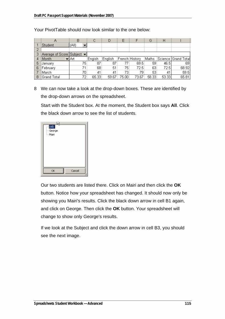
Draft PC Passport Support Materials (November 2007)
Your PivotTable should now look similar to the one below:
8 We can now take a look at the drop-down boxes. These are identified by
the drop-down arrows on the spreadsheet.
Start with the Student box. At the moment, the Student box says All. Click
the black down arrow to see the list of students.
Our two students are listed there. Click on Mairi and then click the OK
button. Notice how your spreadsheet has changed. It should now only be
showing you Mairi's results. Click the black down arrow in cell B1 again,
and click on George. Then click the OK button. Your spreadsheet will
change to show only George's results.
If we look at the Subject and click the down arrow in cell B3, you should
see the next image.
Spreadsheets Student Workbook — Advanced 115

Draft PC Passport Support Materials (November 2007)
All the Subjects have ticks in them. Click on a tick and it will disappear. Try
un-ticking a few of the subjects. Then click the OK button to see what
happens.
The Month list in cell A4 shows a similar list with ticks in them. Un-tick a
month and see the results when you click OK.
Exercise 16: Using PivotTables
Change the type of PivotTable Report. From the PivotTable toolbar, click the
PivotTable button. From the menu that pops up, select Format Report. Click
on any of the formats you like then click OK to see what happens. If you don't
like what you see, click Edit > Undo AutoFormat to get back to your
PivotTable.
Using Goal Seek Occasionally you may know the result you want to achieve from a formula, but
don’t know what the input values have to be to achieve it. On these
occasions, you can make use of the goal seek utility.
Spreadsheets Student Workbook — Advanced 116

Draft PC Passport Support Materials (November 2007)
For example, suppose you want to know how many units must be sold to
achieve a profit of £1,000,000. You can use goal seek to find this out. To
calculate this, goal seek has to know:
♦ the cell that contains the formula that calculates the profit
♦ the profit value you want to achieve
♦ the cell containing the value to be adjusted by goal seek.
How to Use Goal Seek 1 Select the Tools, Goal Seek menu option.
2 Complete the dialogue box:
♦ Set cell: Enter the reference of the cell that's to be set to a specific
value. This will initially be set to the cell containing the active cell
pointer.
♦ To value: Enter the specific value that's to be shown in the cell
identified in the Set cell text box.
♦ By changing cell: Enter the reference of the cell that's to be changed
to achieve the value specified in the To value text box.
3 Click OK.
Excel will perform the necessary calculations and then the Goal Seek Status dialogue box will be displayed showing a solution.
The result of Excel’s calculations will be shown in this dialogue box and in
the specified cells on the worksheet.
4 Either accept or abandon the suggested changes.
To accept the result of the goal seek, click OK. The changes will remain in
the cells on the worksheet.
Or
To abandon the changes and return to the original cell contents, click
Cancel.
Spreadsheets Student Workbook — Advanced 117

Draft PC Passport Support Materials (November 2007)
Exercise 17: Using Scenarios
What If Scenario
You are considering a number of loan options for a car, and wish to calculate
the monthly repayments that would be due for the various options. You can
use scenarios to do this — to see what will happen if different loans/interest
rates/payback periods are applied. By changing the input values to a function,
you can find out what the result will be — the monthly payment in this
example. The options are:
Amount of Loan Interest Rate Payback Period
Option 1 £22,000 7% 5 years
Option 2 £25,000 8% 8 years
Option 3 £30,000 10% 12 years
1 On a new worksheet, input the option 1 data and use the =PMT function to
calculate the monthly repayment on this option. (£435.63)
2 Open the Tools menu, choose Scenarios, and set up the three scenarios
— one for each option in the table above. They will be listed in the
Scenario Manager dialogue box.
3 Show each of the scenarios in turn — you are looking for the one with the
lowest monthly repayments, as you are tight for cash on a day-to-day
basis.
4 Which option will cost least each month?
You will notice that only one scenario can be displayed at a time — so you
have to keep switching between them to compare one with the other.
If you wish to display the results of each scenario side-by-side so you can
compare them more easily, you can use a scenario summary.
5 Create a scenario summary for your options (choose Summary from the
Scenario Manager dialogue box).
Spreadsheets Student Workbook — Advanced 118

Draft PC Passport Support Materials (November 2007)
Sorting Data To change the order in which data is displayed, you can use the Sort Ascending (a–z, 0–9) and Sort Descending (z–a, 9–0) buttons shown on
the Standard toolbar. Using these buttons you can simply place the active cell
pointer in the column to be used in the sort and then click the Sort Ascending or Sort Descending button.
For example, to sort the data below in ascending order of Invoice No, you
would click in the Invoice No column and then click the Sort Ascending
button.
The data would then be shown in ascending order of Invoice No.
For best results, the range you sort should have column labels, or headers.
Spreadsheets Student Workbook — Advanced 119

Draft PC Passport Support Materials (November 2007)
1 Click a cell in the range you want to sort.
2 On the Data menu, click Sort.
3 In the Sort by and Then by boxes, click the columns you want to sort,
starting with the most important.
4 Select any other sort options you want, and then click OK.
Spreadsheets Student Workbook — Advanced 120

Draft PC Passport Support Materials (November 2007)
Exercise 18: Sorting
1 Open the Stock Records workbook stored in the Databases folder in your
WorkStuff folder.
2 Follow the instructions below to sort the product list in ascending order of
Location.
♦ Move the cell pointer onto a cell in the Location column.
♦ Click the Sort Ascending button shown on the Standard toolbar.
3 Now sort the list in order of supplier name by clicking in that column and
clicking the Sort Ascending button.
4 Sort the list in descending order of product name.
5 Sort the list in ascending order of cost price.
6 Sort it in descending order of location.
7 Save and close the workbook.
Using Lists If you keep lists (a series of worksheet rows that contain related data) of
information such as customer invoices, product details or simply names and
addresses, you can enter these onto a worksheet and then use Excel’s list
management facilities to organise and analyse the data. Lists are sometimes
referred to as databases.
You can, for example, sort the list to show the data in a specific order, extract
some of the information, create a summary report or perform calculations
using the data in the list.
Before entering your list into a worksheet, you should plan its content and
structure.
Spreadsheets Student Workbook — Advanced 121

Draft PC Passport Support Materials (November 2007)
In a separate row at the top of each column, you should enter a column label
to identify the field in that column. It’s advisable to format the column labels in
a different way to the data in the list so that Excel doesn't include it as part of
the data in the list.
Each of the other rows in the list contains all the fields for one invoice. This is
referred to as a record.
There are a few rules you should follow when creating a list:
♦ Always enter column labels on the top row of the list, applying some
formatting attributes to differentiate between the column labels and the
data in the list.
♦ The first record must appear on the first row beneath the column labels.
Use cell borders to draw lines below labels if required — don’t insert extra
rows.
♦ Avoid putting more than one list on a single worksheet as some of Excel’s
list management features, such as filtering, can be used on only one list at
a time.
♦ Leave at least one blank column and row between the list and other data
on the same worksheet.
♦ Don’t put spaces at the beginning of a cell entry — this can cause
problems when filtering or sorting the data.
Spreadsheets Student Workbook — Advanced 122

Draft PC Passport Support Materials (November 2007)
AutoFilter Drop-downs One of the common things that you do with data in Excel is to filter the data
based on different field values. To make this functionality available to you
when using lists, AutoFilter drop-downs are automatically added in the header
row of a list when the list is created. This enables you to look up specific
values by picking the appropriate drop-down list value you wish to see — all
records for that value are returned.
Using a Data Form When working with lists, you can use the Data, Form command to display a
form to make data entry user-friendlier. Using this form you can modify, find,
add and/or delete records from your list.
Furthermore, you can use the Criteria button to search for particular records
in the list. When you click this button, a blank form is displayed. Type an
example of the records you're looking for and then click either the Find Prev
or Find Next button to find a record based on the example you gave.
Exercise 19: Using Lists
1 Create a new workbook.
2 Enter the column labels and two records as shown below.
Notice that the list starts on row 6 and the column labels have been
formatted as bold. Column H should contains formulas to calculate
Selling Price 2 by multiplying Selling Price 1 by 120%. Where necessary,
increase the column width.
Spreadsheets Student Workbook — Advanced 123

Draft PC Passport Support Materials (November 2007)
3 Save the workbook as Stock List and store it in the Databases folder in
your WorkStuff folder.
4 Make sure the cell pointer is within the list and then choose the Data, Form menu option. This displays a form you can use to work with the
existing records in your list and to add new records.
5 Following the instructions below, use the data form to make some changes
to the list.
♦ Change the entry in the Selling Price 1 box to 59.6 and then press
[Enter] to apply the change.
The Selling Price 2 entry in the worksheet changes as its formula uses
the Selling Price 1 you've just altered and the second record from your
list is displayed in the data form.
♦ Click the Delete button and then click OK to confirm that you want to
delete this record.
Now you’ll add a new record to the list using the data form.
♦ As a blank form is displayed after you deleted the second record, you
can create a new record by typing in this blank form. Complete it as
shown below.
♦ Press [Enter] to add this record to the list. Notice that the formula is
copied from the previous record in the list.
♦ Click Find Prev in the data form to return to the first record in the list.
♦ Click Find Next to display the second record.
Spreadsheets Student Workbook — Advanced 124

Draft PC Passport Support Materials (November 2007)
♦ Click the Close button to return to the workbook.
6 Save and close the workbook.
Using Filters Filters are used to display only those records in your list that match specified
criteria. For example, you may want to see only those customers whose name
is Smith. As only the records relating to Smith will be shown, it will be easier
to compare and review the data.
Using Excel’s AutoFilter utility, you can view a subset of the records in your
list by selecting or specifying the required criteria
Before you can set a filter, you must switch on AutoFilter. To do this, make
sure that the active cell pointer is within the list and then select the Data,
Filter, AutoFilter menu option. Filter arrows will then be displayed to the right
of the column labels.
Once you have switched on AutoFilter, you can select or set conditions by
choosing from the drop-down list for each field. For example, if you wanted to
see only those products that are located at the Carrick warehouse, you would
choose Carrick from the Location drop-down list.
Spreadsheets Student Workbook — Advanced 125

Draft PC Passport Support Materials (November 2007)
The records that match your choice will be displayed in the list; the others will
be hidden.
On screen, the Location drop-down arrow and the selected row numbers are
highlighted in blue to indicate that a filter has been set.
You can reduce the list further by setting a condition for another field, eg for
those products supplied by Davidson House Furnishings.
The records now shown are for products that are located at the Carrick
warehouse and are supplied by Davidson House Furnishings.
Cancelling a Filter Once a filter has been set for a field, you can cancel it by selecting the (All) option from the field’s drop-down list. If, however, you have set filters on a
number of fields and you want to cancel all of them, the quickest way to do so
is to choose the Data, Filter, Show All menu option. Using this command
means that you don’t have to cancel the filters one at a time.
Setting a Custom Filter In addition to choosing cell contents from a filter’s drop-down list, you can set
a custom filter using wildcard characters (* and ?) and/or operators such as
greater than (>) and less than (<).
First display the Custom AutoFilter box by choosing Custom from a field’s
filter drop-down list, then specify the criteria for this field. In the example that
follows, the custom filter will display all the chairs and tables in this list (you
use or rather than and in this box because the name should contain chair or table).
Spreadsheets Student Workbook — Advanced 126

Draft PC Passport Support Materials (November 2007)
Using Advanced Filters If you want to apply a filter that uses more than the two criteria allowed by the
Custom AutoFilter dialogue box, you will have to use the Advanced Filter options. For example, using the list from the previous exercise, you may want
to list all chairs, tables and cabinets.
Another instance where you would have to use these options would be where
you want a field to be compared to the result of a calculation. For example,
you might want to list the products whose profit (calculated by subtracting
Cost Price from Selling Price 2) is greater than £50.
Creating Criteria Ranges The first step in using the advanced filter options is to create a criteria range.
This range of cells contains the name of the field(s) that you want to test and
the value(s) to be used for the comparison(s).
The first row in the range must contain the column label of the field(s) to be
compared. The second and subsequent rows are used to specify the criteria
to be met.
Note: Criteria ranges must span at least two rows.
Spreadsheets Student Workbook — Advanced 127

Draft PC Passport Support Materials (November 2007)
When all the criteria appear in a single row, as they do above, only those
records matching all criteria will be listed. If you want to list the records that
match at least one of the criteria, they must appear on separate rows.
Note: You can use the wildcard character * to replace any number of
characters in your criteria, and ? to replace a single character. In the example
above, *dining* means the product name should contain the word dining,
perhaps with some characters before it and/or some characters after it.
If you want to test the same field for more than one condition, the field can be
repeated in the criteria range. For example, if you wanted to list those
products whose Cost Price is more than £20 and less than £50, the criteria
range would be:
with Cost Price appearing twice on the same row.
Applying Advanced Filters Once you have created the criteria range, you can apply the filter using the
Data, Filter, Advanced Filter command, which will display the Advanced Filter dialogue box.
Note: The cell pointer must be within the list before you select this command.
Spreadsheets Student Workbook — Advanced 128

Draft PC Passport Support Materials (November 2007)
Using the options under Action you can choose to copy the filtered list in
another part of the worksheet rather than where the full list is located, and you
can prevent duplicated records being included in the filtered list by ticking the
Unique records only box.
The List range will be completed by Excel, so you need only specify the
Criteria range and, if necessary, the location for the filtered list in the Copy to text box, before clicking OK.
The filtered list will be displayed, with those records not matching the required
criteria hidden or, if you chose the Copy to another location option, in the
part of the worksheet you specified.
Note: If you use the Copy to another location option, you can choose to
show only some of the fields in the filtered list. For example, you may be
interested in only the product name, supplier and cost price rather than all the
fields in the original list.
You can do this by copying the column labels of those fields you do want in
the filtered list to the range where the filtered list is to be shown. You would
then select this range as the Copy to range in the Advanced Filter dialogue
box.
Exercise 20: Using Filters
1 Open the Stock Records workbook stored in the Databases folder in your
WorkStuff folder.
This workbook has the same layout as the one you created in Exercise 19
but has more records.
2 Ensure the cell pointer is in the list and then select the Data, Filter, AutoFilter menu option to display the filter arrows at the right of the
column labels.
Spreadsheets Student Workbook — Advanced 129

Draft PC Passport Support Materials (November 2007)
3 Display only those products located at the Calderwood warehouse by
selecting Calderwood from the Location field’s drop-down list.
All the other records are hidden, leaving only the Calderwood stock in this
list.
4 Reduce the list further by displaying only those products supplied by
Palteck Furnishings.
Now the only records displayed are those held at the Calderwood
warehouse that have been supplied by Palteck. Notice the blue colour on
the filter arrows of those columns that have been filtered and also on the
row numbers.
5 Select the Data, Filter, Show All menu option to display all the products
again.
6 Display only Lazy Chairs stored in the Carrick warehouse.
7 Select (All) from the Product Name field's drop-down list so that all the
products stored in the Carrick warehouse are shown in the list.
8 Experiment with the filters to display different subsets of the records.
9 Display all records using the Data, Filter, Show All menu option.
10 Follow the instructions below to set a custom filter that will display all
product codes that start with the letter K.
♦ From the Product Code drop-down list, select (Custom).
♦ Select begins with from the criterion drop-down list.
Spreadsheets Student Workbook — Advanced 130

Draft PC Passport Support Materials (November 2007)
♦ Type K into the Custom AutoFilter dialogue box as shown below.
♦ Click OK to apply the filter.
11 Following the instructions below, modify the filter so that all products with
codes beginning with K or M will be shown in the list.
♦ Select (Custom) from the Product Code drop-down list.
♦ Ensure that K still appears as the first criterion.
♦ Click the Or option button, then select the begins with operator from
the second criterion drop-down list.
♦ Enter M into the second criterion text box.
♦ Click OK to apply the filter.
Product codes starting with either K or M are now shown in the list.
12 Display all records.
13 Use a custom filter to display all products whose Cost Price is greater than £50.
14 Display all the records.
15 Display a list of those products stored at the Carrick warehouse, then use
a custom filter to display only those products that have been allocated at
least once.
16 Use the Data, Filter, Show All command to display all records.
17 Print the workbook on one landscape page. Remember to add your name
to the footer.
18 Save the changes you’ve made and close the workbook.
Spreadsheets Student Workbook — Advanced 131

Draft PC Passport Support Materials (November 2007)
Using Functions with Lists and Filters When you use the SUM function with a list, it totals all the values you’ve
specified. However, if you apply a filter to the list, the SUM function still totals
all the values, regardless of the filter. The SUBTOTAL function is a multi-
purpose function that can give you the equivalent of the SUM, AVERAGE,
MAX, MIN, COUNT and COUNTA functions, amongst others, but using only
the values that are displayed by the filter at that time.
SUBTOTAL Function The syntax of the SUBTOTAL function is:
=SUBTOTAL(function_number, range)
The function_number argument comes from this list:
Function_number Function 1 AVERAGE
2 COUNT
3 COUNTA
4 MAX
5 MIN
6 PRODUCT
7 STDEV
8 STDEVP
9 SUM
10 VAR
11 VARP
Example
This illustration shows a list where the Cost Price column is to be totalled.
However, the total should change to include only the displayed records when
the list is filtered.
Spreadsheets Student Workbook — Advanced 132

Draft PC Passport Support Materials (November 2007)
To total the Cost Price column the function would read =SUBTOTAL(9, D3:D16). The function number 9 has been used as this is the SUM function.
To find the average cost price the function would be =SUBTOTAL(1, D3:D16) since function number 1 is AVERAGE.
Forecast Function This function calculates, or predicts, a future value by using existing values.
The predicted value is a y-value for a given x-value. The known values are
existing x-values and y-values, and the new value is predicted by using linear
regression. You can use this function to predict future sales, inventory
requirements, or consumer trends.
Syntax
FORECAST(x,known_y's,known_x's)
This returns the correlation coefficient of the array1 and array2 cell ranges.
Use the correlation coefficient to determine the relationship between two
properties. For example, you can examine the relationship between a height
in metres and the speed of impact of an object.
Syntax
CORREL(array1,array2)
Array1 is a cell range of values.
Array2 is a second cell range of values.
Spreadsheets Student Workbook — Advanced 133

Draft PC Passport Support Materials (November 2007)
Lookup Function If you wanted to find a specific value in a spreadsheet, you might use a
Lookup function, for example to find a phone extension, or a sales amount or
product. After you look up the data, you can perform calculations or display
results with the values returned. There are several ways to look up values in a
list of data and to display the results.
There are different functions to perform different types of lookups. The two
most common are VLOOKUP and HLOOKUP but you could also use Index,
Match and Offset functions.
VLOOKUP V (Vertical) LOOKUP looks for values vertically in a list by using an exact
match or an approximate match. VLOOKUP searches for a value in the first
column of a table array and returns a value in the same row from another
column in the table array. Use VLOOKUP instead of HLOOKUP when your
comparison values are located in a column to the left of the data that you want
to find.
Syntax VLOOKUP(lookup_value, table_array, col_index_num, range_lookup)
Understanding the parts of the function
Lookup_value The value to search in the first column of the table array which
could be a value or a reference. If lookup value is smaller than the smallest
value in the first column of table array, VLOOKUP returns the #N/A error
value.
Table_array Two or more columns of data. Use a reference to a range or a
range name. The values in the first column of table array are the values
searched by lookup value. These values can be text, numbers, or logical
values. Uppercase and lowercase texts are equivalent.
Col_index_num The column number in the table array from which the
matching value must be returned. A col_index_num of 1 returns the value in
the first column in table array; a col_index_num of 2 returns the value in the
second column in table array, and so on.
Spreadsheets Student Workbook — Advanced 134

Draft PC Passport Support Materials (November 2007)
If col_index_num is less than 1, VLOOKUP returns the #VALUE! error value.
If col_index_num is greater than the number of columns in table array,
VLOOKUP returns the #REF! error value.
Range_lookup A logical value that specifies whether you want VLOOKUP to
find an exact match or an approximate match. If the logical value is TRUE or
omitted, an exact or approximate match is returned. If an exact match is not
found, the next largest value that is less than lookup_value is returned.
Note: The values in the first column of table array must be placed in
ascending sort order; otherwise, VLOOKUP may not give the correct value.
You can put the values in ascending order by choosing the Sort command
from the Data menu and selecting Ascending.
If the logical value is FALSE, VLOOKUP will only find an exact match. In this
case, the values in the first column of table array do not need to be sorted. If
there are two or more values in the first column of table array that match the
lookup value, the first value found is used. If an exact match is not found, the
error value #N/A is returned.
HLOOKUP H (Horizontal) LOOKUP looks up values horizontally in a list by using an exact
match or an approximate match. HLOOKUP searches for a value in the top
row of a table or an array of values, and then returns a value in the same
column from a row you specify in the table or array. Use HLOOKUP when
your comparison values are located in a row across the top of a table of data,
and you want to look down a specified number of rows.
Syntax
HLOOKUP(lookup_value, table_array, row_index_num, range_lookup)
Lookup_value is the value to be found in the first row of the table.
Lookup_value can be a value, a reference, or a text string.
Table_array is a table of information in which data is looked up. Use a
reference to a range or a range name. The values in the first row of
table_array can be text, numbers, or logical values.
Spreadsheets Student Workbook — Advanced 135

Draft PC Passport Support Materials (November 2007)
Row_index_num is the row number in table_array from which the matching
value will be returned. A row_index_num of 1 returns the first row value in
table_array, a row_index_num of 2 returns the second row value in
table_array, and so on. If row_index_num is less than 1, HLOOKUP returns
the #VALUE! error value; if row_index_num is greater than the number of
rows on table_array, HLOOKUP returns the #REF! error value.
Range_lookup is a logical value that specifies whether you want HLOOKUP
to find an exact match or an approximate match. If TRUE or omitted, an
approximate match is returned. In other words, if an exact match is not found,
the next largest value that is less than lookup_value is returned. If FALSE,
HLOOKUP will find an exact match. If one is not found, the error value #N/A is
returned.
Note: Uppercase and lowercase text is equivalent. You can put values in
ascending order, left to right, by selecting the values and then clicking Sort on
the Data menu. Click Options, click Sort left to right, and then click OK.
Under Sort by, click the row in the list, and then click Ascending.
You can also use the Help files on your spreadsheet program to find out more
about these other functions.
Lookup and Reference Functions Function Description ADDRESS Returns a reference as text to a single cell in a worksheet
AREAS Returns the number of areas in a reference
CHOOSE Chooses a value from a list of values
COLUMN Returns the column number of a reference
COLUMNS Returns the number of columns in a reference
GETPIVOTDATA Returns data stored in a PivotTable
HLOOKUP Looks in the top row of an array and returns the value of the indicated cell
HYPERLINK Creates a shortcut or jump that opens a document stored on a network server, an intranet, or the internet
INDEX Uses an index to choose a value from a reference or array
INDIRECT Returns a reference indicated by a text value
LOOKUP Looks up values in a vector or array
Spreadsheets Student Workbook — Advanced 136
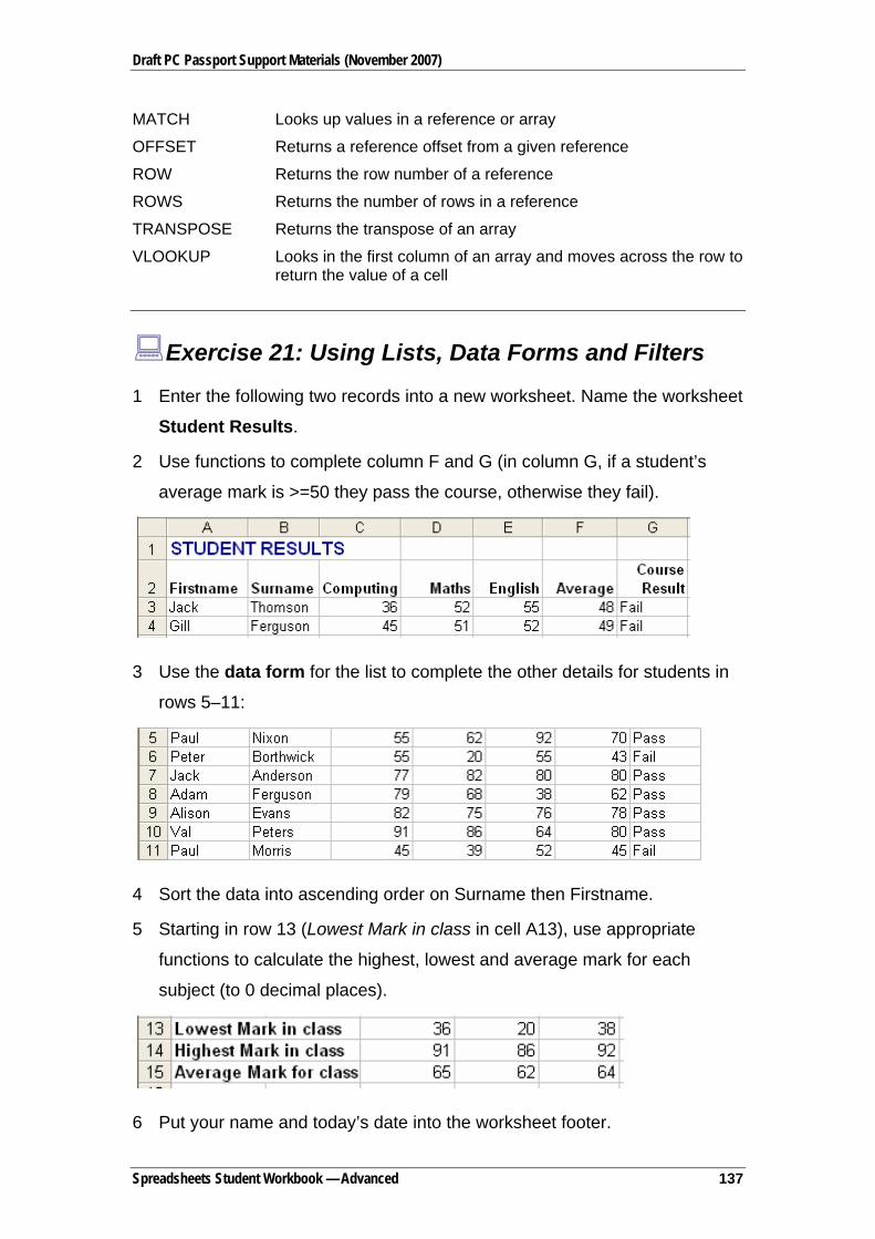
Draft PC Passport Support Materials (November 2007)
MATCH Looks up values in a reference or array
OFFSET Returns a reference offset from a given reference
ROW Returns the row number of a reference
ROWS Returns the number of rows in a reference
TRANSPOSE Returns the transpose of an array
VLOOKUP Looks in the first column of an array and moves across the row to return the value of a cell
Exercise 21: Using Lists, Data Forms and Filters
1 Enter the following two records into a new worksheet. Name the worksheet
Student Results.
2 Use functions to complete column F and G (in column G, if a student’s
average mark is >=50 they pass the course, otherwise they fail).
3 Use the data form for the list to complete the other details for students in
rows 5–11:
4 Sort the data into ascending order on Surname then Firstname.
5 Starting in row 13 (Lowest Mark in class in cell A13), use appropriate
functions to calculate the highest, lowest and average mark for each
subject (to 0 decimal places).
6 Put your name and today’s date into the worksheet footer.
Spreadsheets Student Workbook — Advanced 137

Draft PC Passport Support Materials (November 2007)
7 Format the worksheet effectively.
8 Save the worksheet and print it out — in data view.
e row and column
10
iltering
e Students Result worksheet to practise filtering data lists. Use
s where the student surname is Ferguson.
tween 50 and 80
dvanced Filter
ced Filter option to display those students who:
in computing
9 Then print the worksheet out in Formula view, with th
headings and gridlines displayed. The printout should fit onto one page.
Close the workbook.
F
1 Use th
AutoFilter for this.
♦ Display all record
♦ Display all records where the maths mark was >=55.
♦ Display all records where the student result was Fail.
♦ Display all records where the computing result was be
(inclusive).
A
1 Use the Advan
♦ passed computing but failed the course
♦ achieved 65 or more in each subject
♦ scored between 50 and 70 (inclusive)
♦ averaged either below 50 or 80 and above.
Finally should (after consultation with their tutor) be able to do the
ning Outcomes for the PC Passport Spreadsheet
The candidate
assessment for this Unit.
This completes all the lear
subject. Microsoft Excel is one of a range of spreadsheets that could be used
to achieve the same results.
Spreadsheets Student Workbook — Advanced 138


![5 refreshed PC Passport [Read-Only] · PC Passport (Intermediate) unitsPC Passport (Intermediate) units IT Systems 5 F1FA 11 0.5 IT Software - Spreadsheets 5 F1FC 11 1 and Database](https://img.pdfslide.us/doc/110x75/5fd402c3a70543283605b610/5-refreshed-pc-passport-read-only-pc-passport-intermediate-unitspc-passport.jpg)