PC-ORD

TM

Multivariate Analysis of Ecological Data

Version 6User’s Booklet

2

Suggested citation: McCune, B. and M. J. Mefford. 2011. PC-ORD. Multivariate Analysis of Ecological Data. Version 6. MjM Software, Gleneden Beach, Oregon, U.S.A.

Cover: The essence of multivariate analysis is the extraction of a small number of important relationships from a very large number of possible relationships.

Waiver: Although the software has been carefully tested, the user accepts and uses the program material as it is, at the user’s own risk, relying solely upon his/her own inspection of the program material and without reliance upon any representation or description concerning the program material. Neither MjM Software Design nor associated individuals make any expressed or implied warranty of any kind with regard to the program material, and shall have no liability or responsibility to any recipient with respect to any liability, loss, or damage that directly or indirectly arises out of the use of the disk and the programs and/or subroutines contained on the disk, including, but not limited to, any loss of business or loss of data or other incidental or consequential damages. By using this software you agree to this.

© 1991, 1993, 1995, 1997, 1999, 2006, 2011 MjM Software Design© 1991, 1993, 1995, 1997, 1999, 2006, 2011 Bruce McCuneAll rights reserved. Printed in the United States of America.

3

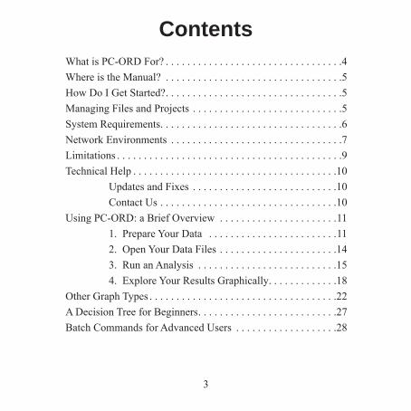
ContentsWhat is PC-ORD For? . . . . . . . . . . . . . . . . . . . . . . . . . . . . . . . . .4Where is the Manual? . . . . . . . . . . . . . . . . . . . . . . . . . . . . . . . . .5How Do I Get Started?. . . . . . . . . . . . . . . . . . . . . . . . . . . . . . . . .5Managing Files and Projects . . . . . . . . . . . . . . . . . . . . . . . . . . . .5System Requirements. . . . . . . . . . . . . . . . . . . . . . . . . . . . . . . . . .6Network Environments . . . . . . . . . . . . . . . . . . . . . . . . . . . . . . . .7Limitations . . . . . . . . . . . . . . . . . . . . . . . . . . . . . . . . . . . . . . . . . .9Technical Help . . . . . . . . . . . . . . . . . . . . . . . . . . . . . . . . . . . . . .10

Updates and Fixes . . . . . . . . . . . . . . . . . . . . . . . . . . .10Contact Us . . . . . . . . . . . . . . . . . . . . . . . . . . . . . . . . .10

Using PC-ORD: a Brief Overview . . . . . . . . . . . . . . . . . . . . . .111. Prepare Your Data . . . . . . . . . . . . . . . . . . . . . . . .112. Open Your Data Files . . . . . . . . . . . . . . . . . . . . . .143. Run an Analysis . . . . . . . . . . . . . . . . . . . . . . . . . .154. Explore Your Results Graphically. . . . . . . . . . . . .18

Other Graph Types . . . . . . . . . . . . . . . . . . . . . . . . . . . . . . . . . . .22A Decision Tree for Beginners. . . . . . . . . . . . . . . . . . . . . . . . . .27Batch Commands for Advanced Users . . . . . . . . . . . . . . . . . . .28

4

What is PC-ORD For?PC-ORD is a Windows program for multivariate analysis of ecological data

entered in spreadsheets. The terminology in the software is tailored for ecologists. We emphasize nonparametric tools, graphical representation, and randomization tests for analysis of community data. In addition to utilities for transforming data and managing fi les, PC-ORD offers many ordination and classifi cation techniques not available in major statistical packages including: CCA, DCA, MRPP, perMANOVA, two-way clustering, TWINSPAN, Beals smoothing, diversity indices, species lists, Mantel test, many ordination overlay methods (quantitative, symbol-coding, color-coding, grid, joint plot, biplot, successional vector), various rotation methods, 3D ordination graphics, indicator species analysis, Bray-Curtis ordination, city-block distance measures, species-area curves, tree data summaries, publication-quality dendrograms, and autopilot NMS.

Very large data sets can be analyzed. Most operations accept a matrix up to 32,000 rows or 32,000 columns and up to 536,848,900 matrix elements, provided that your computer has adequate memory.

Virtually any multivariate data set consisting of a set of entities, each with a number of measured attributes, is adaptable to PC-ORD. In community ecology, the fi rst matrix will often contain species abundance data in a set of samples. The possible formats for entering these data can be found in Data Preparation in the software help system. In addition to this main matrix, a second matrix, often containing environmental data, can be entered for analysis of its relationship to the fi rst matrix. The inclusion of this second matrix greatly enriches the system’s analytical capabilities. Both matrices are displayed in PC-ORD in fi le viewing windows.

5

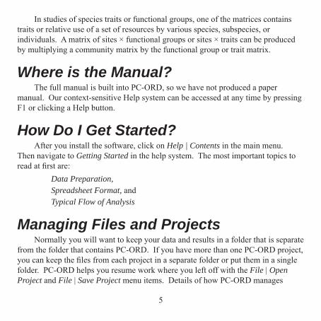
In studies of species traits or functional groups, one of the matrices contains traits or relative use of a set of resources by various species, subspecies, or individuals. A matrix of sites × functional groups or sites × traits can be produced by multiplying a community matrix by the functional group or trait matrix.

Where is the Manual?The full manual is built into PC-ORD, so we have not produced a paper

manual. Our context-sensitive Help system can be accessed at any time by pressing F1 or clicking a Help button.

How Do I Get Started?After you install the software, click on Help | Contents in the main menu.

Then navigate to Getting Started in the help system. The most important topics to read at fi rst are:

Data Preparation, Spreadsheet Format, andTypical Flow of Analysis

Managing Files and ProjectsNormally you will want to keep your data and results in a folder that is separate

from the folder that contains PC-ORD. If you have more than one PC-ORD project, you can keep the fi les from each project in a separate folder or put them in a single folder. PC-ORD helps you resume work where you left off with the File | Open Project and File | Save Project menu items. Details of how PC-ORD manages

6

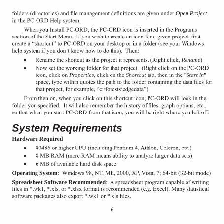
folders (directories) and fi le management defi nitions are given under Open Project in the PC-ORD Help system.

When you Install PC-ORD, the PC-ORD icon is inserted in the Programs section of the Start Menu. If you wish to create an icon for a given project, fi rst create a “shortcut” to PC-ORD on your desktop or in a folder (see your Windows help system if you don’t know how to do this). Then:

Rename the shortcut as the project it represents. (Right click, Rename) Now set the working folder for that project. (Right click on the PC-ORD

icon, click on Properties, click on the Shortcut tab, then in the "Start in" space, type within quotes the path to the folder containing the data fi les for that project, for example, “c:\forests\edgedata”).

From then on, when you click on this shortcut icon, PC-ORD will look in the folder you specifi ed. It will also remember the history of fi les, graph options, etc., so that when you start PC-ORD from that icon, you will be right where you left off.

System RequirementsHardware Required

80486 or higher CPU (including Pentium 4, Athlon, Celeron, etc.) 8 MB RAM (more RAM means ability to analyze larger data sets) 6 MB of available hard disk space

Operating System: Windows 98, NT, ME, 2000, XP, Vista, 7; 64-bit (32-bit mode)Spreadsheet Software Recommended: A spreadsheet program capable of writing fi les in *.wk1, *.xls, or *.xlsx format is recommended (e.g. Excel). Many statistical software packages also export *.wk1 or *.xls fi les.

7

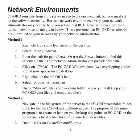
Network EnvironmentsPC-ORD runs fi ne from a fi le server in a network environment, but you must set up the software correctly. Because network environments vary, your network administrator may need to help you set up PC-ORD. Generic instructions for a typical network setup are given below. These presume that PC-ORD has already been installed on your network by your network administrator.Method 1

1. Right click on some free space on the desktop.2. Select: New | Shortcut3. Enter the path for pcord6.exe. Or use the Browse button to fi nd this

executable fi le. Your network administrator can provide this path.4. Click on “Finish”. The PC-ORD Windows icon (two overlapping circles)

should now appear on the desktop.5. Right click on the PC-ORD icon.6. Select: Properties | Shortcut7. Under “Start in” enter your working folder (where you will keep your

PC-ORD data fi les and temporary fi les).Method 2

1. Navigate in the fi le system of the server to the PC-ORD executable folder. Look for the fi le CreateDesktopShortcut.exe. The purpose of this mini-program is to create an icon on you desktop that points to PC-ORD on the server and a local folder for storing your temporary fi les.

2. Double click on CreateDesktopShortcut.

8

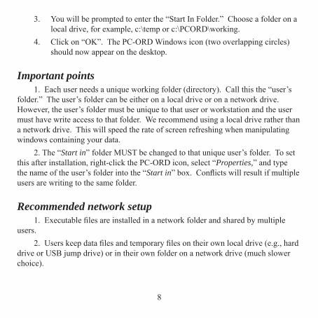
3. You will be prompted to enter the “Start In Folder.” Choose a folder on a local drive, for example, c:\temp or c:\PCORD\working.

4. Click on “OK”. The PC-ORD Windows icon (two overlapping circles) should now appear on the desktop.

Important points1. Each user needs a unique working folder (directory). Call this the “user’s

folder.” The user’s folder can be either on a local drive or on a network drive. However, the user’s folder must be unique to that user or workstation and the user must have write access to that folder. We recommend using a local drive rather than a network drive. This will speed the rate of screen refreshing when manipulating windows containing your data.

2. The “Start in” folder MUST be changed to that unique user’s folder. To set this after installation, right-click the PC-ORD icon, select “Properties,” and type the name of the user’s folder into the “Start in” box. Confl icts will result if multiple users are writing to the same folder.

Recommended network setup1. Executable fi les are installed in a network folder and shared by multiple

users.2. Users keep data fi les and temporary fi les on their own local drive (e.g., hard

drive or USB jump drive) or in their own folder on a network drive (much slower choice).

9

For class use1. Same as above, but each user should copy the data fi les provided for the

class into their own folders.2. In computer classrooms, users may want to defi ne their “Start in” folder as

a removable drive, such as a jump drive. This allows users to preserve their own settings from one session to the next, regardless of which machine they are using.

LimitationsMost of the programs in PC-ORD for Windows can accept a matrix up to 32,000 rows or 32,000 columns, provided that you have adequate memory installed in your machine. For all analyses, the following limits apply:

rows x columns ≤ 536,848,900 rows ≤ 32,000 (23,170 if a square distance matrix is calculated) columns ≤ 32,000 (23,170 for PCA)The actual limits will depend on the particular analysis being used. For

example all analyses that require a square distance matrix (Cluster Analysis, MRPP, NMS, perMANOVA, etc.), the maximum number of rows is 23,170.

You can evaluate your memory needs with the Memory Requirements utility provided under the File menu.

If you do encounter an “out of memory” error, and you do not have an exceptionally large data set, then a memory allocation error may have occurred. In this case, close out all programs, go through your normal shut-down procedure, restart, then try to rerun your analysis in PC-ORD.

10

Technical HelpWe use email to answer technical questions about the software from registered

users. Our software support pertains only to programs obtained directly from MjM Software Design.

If you experience unexpected behavior, often someone else will have detected the same problem and it will already be fi xed. So before you contact us… Please download the latest fi xes from our website <www.pcord.com>, and

determine whether the problem still exists in the latest version. Check the Frequently Asked Questions (FAQ) section on our website. Determine the version you are using by checking the title bar of the PC-ORD

menu or inspecting the header at the top of your output fi les. Please include the full version number in your correspondence with us, specifying not just “version 6” but “version 6.05” or whatever exact version you are using.

Updates and FixesFixes will be posted on the MjM website as needed. PC-ORD maintenance

fi xes are free and can be downloaded from the MjM website: <www.pcord.com>.Click on Help | Internet Support for the current web addresses for this and other aspects of internet support.

Contact UsMjM Website: http://www.pcord.com Email: mjm@centurytel.netFax: 541-764-3935 Phone (orders only): 1-800-690-4499Mail: MjM Software Design, PO Box 129, Gleneden Beach, OR 97388 U.S.A.

11

Using PC-ORD: a Brief OverviewYou can quickly learn the basics of PC-ORD by following four steps:

1. Prepare your data. 2. Open PC-ORD and your data fi les. 3. Run an analysis.4. Explore your results graphically.

1. Prepare Your Data For an easy start, follow the instructions in the help system exactly.A. Put your data in a spreadsheet (e.g. Excel) with the sample units as rows and

variables as columns. Assign a short name to each row and column.B. Your variables will be partitioned into two fi les, one with response variables

(main matrix; e.g., species presence, abundance, or other measure of performance) and the other with predictors or correlates or controlling factors (second matrix; e.g., environmental variables or design variables). PC-ORD will split the data set for you.

C. Start PC-ORD.D. File | Import MatrixE. Choose Main Matrix or Second Matrix, depending on whether you are

importing dependent variables (response variables) or predictors or correlates of the response variables. You can do each set of variables, in sequence.

F. Choose Excel Simple Spreadsheet in the Import File Type dialog.G. Navigate to the fi le that you wish to import and double click on it. You will be

asked to select one worksheet to open.

12

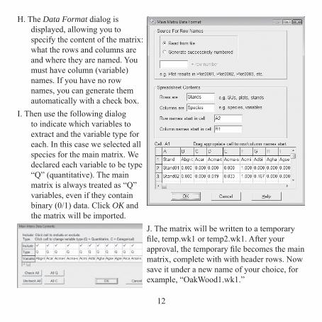
H. The Data Format dialog is displayed, allowing you to specify the content of the matrix: what the rows and columns are and where they are named. You must have column (variable) names. If you have no row names, you can generate them automatically with a check box.

I. Then use the following dialog to indicate which variables to extract and the variable type for each. In this case we selected all species for the main matrix. We declared each variable to be type “Q” (quantitative). The main matrix is always treated as “Q” variables, even if they contain binary (0/1) data. Click OK and the matrix will be imported.

J. The matrix will be written to a temporary fi le, temp.wk1 or temp2.wk1. After your approval, the temporary fi le becomes the main matrix, complete with with header rows. Now save it under a new name of your choice, for example, “OakWood1.wk1.”

13

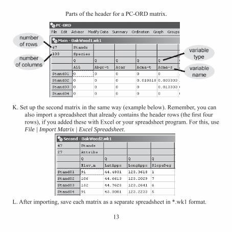
Parts of the header for a PC-ORD matrix.

K. Set up the second matrix in the same way (example below). Remember, you can also import a spreadsheet that already contains the header rows (the fi rst four rows), if you added these with Excel or your spreadsheet program. For this, use File | Import Matrix | Excel Spreadsheet.

L. After importing, save each matrix as a separate spreadsheet in *.wk1 format.

14

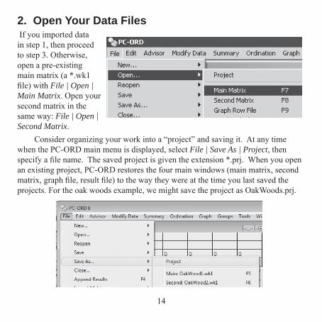
2. Open Your Data Files If you imported data in step 1, then proceed to step 3. Otherwise, open a pre-existing main matrix (a *.wk1 fi le) with File | Open | Main Matrix. Open your second matrix in the same way: File | Open | Second Matrix.

Consider organizing your work into a “project” and saving it. At any time when the PC-ORD main menu is displayed, select File | Save As | Project, then specify a fi le name. The saved project is given the extension *.prj. When you open an existing project, PC-ORD restores the four main windows (main matrix, second matrix, graph fi le, result fi le) to the way they were at the time you last saved the projects. For the oak woods example, we might save the project as OakWoods.prj.

15

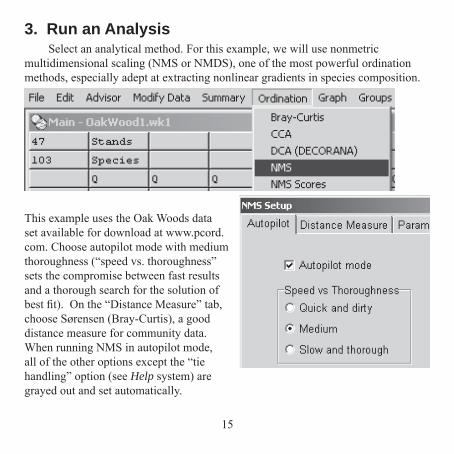
3. Run an Analysis Select an analytical method. For this example, we will use nonmetric

multidimensional scaling (NMS or NMDS), one of the most powerful ordination methods, especially adept at extracting nonlinear gradients in species composition.

This example uses the Oak Woods data set available for download at www.pcord.com. Choose autopilot mode with medium thoroughness (“speed vs. thoroughness” sets the compromise between fast results and a thorough search for the solution of best fi t). On the “Distance Measure” tab, choose Sørensen (Bray-Curtis), a good distance measure for community data. When running NMS in autopilot mode, all of the other options except the “tie handling” option (see Help system) are grayed out and set automatically.

16

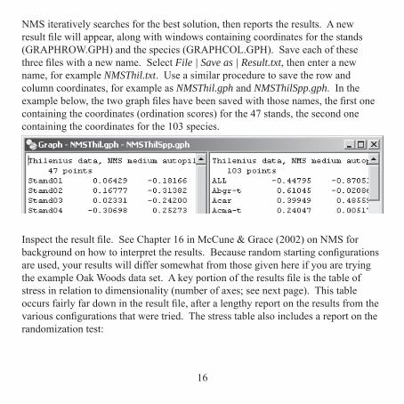
NMS iteratively searches for the best solution, then reports the results. A new result fi le will appear, along with windows containing coordinates for the stands (GRAPHROW.GPH) and the species (GRAPHCOL.GPH). Save each of these three fi les with a new name. Select File | Save as | Result.txt, then enter a new name, for example NMSThil.txt. Use a similar procedure to save the row and column coordinates, for example as NMSThil.gph and NMSThilSpp.gph. In the example below, the two graph fi les have been saved with those names, the fi rst one containing the coordinates (ordination scores) for the 47 stands, the second one containing the coordinates for the 103 species.

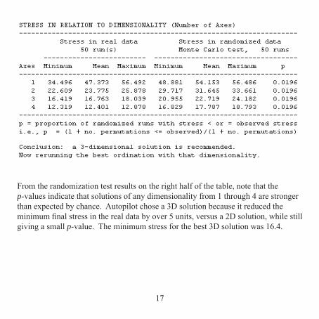
Inspect the result fi le. See Chapter 16 in McCune & Grace (2002) on NMS for background on how to interpret the results. Because random starting confi gurations are used, your results will differ somewhat from those given here if you are trying the example Oak Woods data set. A key portion of the results fi le is the table of stress in relation to dimensionality (number of axes; see next page). This table occurs fairly far down in the result fi le, after a lengthy report on the results from the various confi gurations that were tried. The stress table also includes a report on the randomization test:

17

From the randomization test results on the right half of the table, note that the p-values indicate that solutions of any dimensionality from 1 through 4 are stronger than expected by chance. Autopilot chose a 3D solution because it reduced the minimum fi nal stress in the real data by over 5 units, versus a 2D solution, while still giving a small p-value. The minimum stress for the best 3D solution was 16.4.

18

4. Explore Your Results GraphicallyYou can explore your ordination results with:

2D and 3D ordination graphs Joint plots (Graph | Joint Plot) with variables from the second matrix Determine how much of the variation in the distance matrix is

represented in the ordination diagram (Graph | Statistics | Percent of Variance in Distance Matrix),

Graphically examine the relationships between the ordination and individual variables in the second matrix (Graph | Overlay From Second Matrix),

Calculate linear and rank correlation coeffi cients between axis scores and variables in the second matrix (Statistics | Correlations With Second Matrix),

Rotate the diagram so that major vectors in the joint plot are aligned with the axes (select Graph | Joint plot, then Rotate | By Angle Continuous. Select 5° for the increment and click Next repeatedly to gradually rotate the ordination. See Chapter 15 in McCune and Grace (2002).

Use “successional vectors” to connect before-and-after or other sequential measurements.

Selected examples of these are shown below.

19

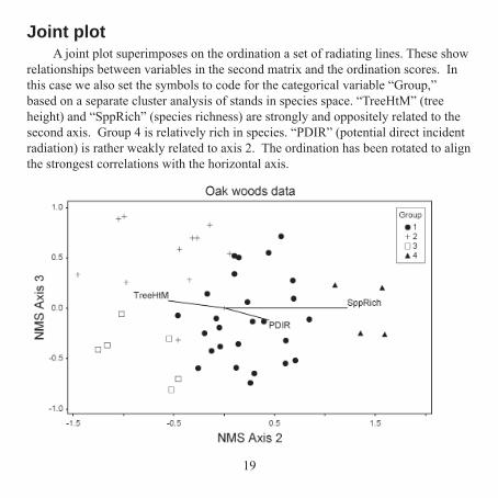
Joint plotA joint plot superimposes on the ordination a set of radiating lines. These show

relationships between variables in the second matrix and the ordination scores. In this case we also set the symbols to code for the categorical variable “Group,” based on a separate cluster analysis of stands in species space. “TreeHtM” (tree height) and “SppRich” (species richness) are strongly and oppositely related to the second axis. Group 4 is relatively rich in species. “PDIR” (potential direct incident radiation) is rather weakly related to axis 2. The ordination has been rotated to align the strongest correlations with the horizontal axis.

20

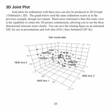
3D Joint PlotJoint plots for ordinations with three axes can also be produced in 3D (Graph

| Ordination | 3D). The graph below used the same ordination scores as in the previous example, though not rotated. Much more informative than this static view is the capability to rotate this 3D picture continuously, allowing you to see the three dimensional structure more clearly. You can save the rotating fi gure as an animated GIF, for use in presentations and web sites (File | Save Animated GIF As).

21

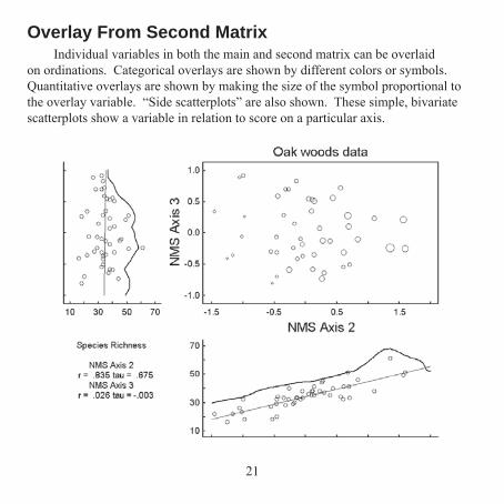
Overlay From Second MatrixIndividual variables in both the main and second matrix can be overlaid

on ordinations. Categorical overlays are shown by different colors or symbols. Quantitative overlays are shown by making the size of the symbol proportional to the overlay variable. “Side scatterplots” are also shown. These simple, bivariate scatterplots show a variable in relation to score on a particular axis.

22

Other Graph TypesThe next few pages illustrate tools in PC-ORD for graphically exploring your

data.

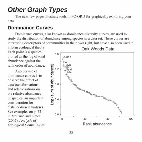
Dominance CurvesDominance curves, also known as dominance-diversity curves, are used to

study the distribution of abundance among species in a data set. These curves are interesting descriptors of communities in their own right, but have also been used to inform ecological theory. Each point is a species plotted as the log of total abundance against the rank order of abundance.

Another use of dominance curves is to observe the effect of data transformations and relativizations on the relative abundance of species, an important consideration for distance-based analyses. See examples on p. 72 in McCune and Grace (2002), Analysis of Ecological Communities.

23

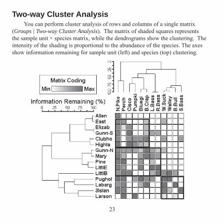
Two-way Cluster AnalysisYou can perform cluster analysis of rows and columns of a single matrix

(Groups | Two-way Cluster Analysis). The matrix of shaded squares represents the sample unit × species matrix, while the dendrograms show the clustering. The intensity of the shading is proportional to the abundance of the species. The axes show information remaining for sample unit (left) and species (top) clustering.

24

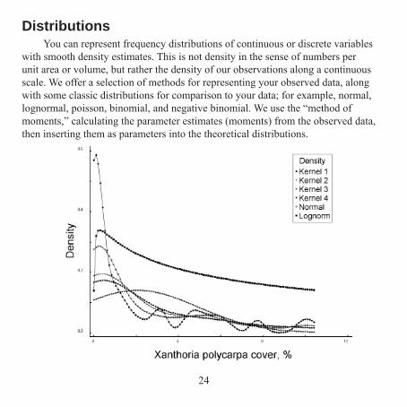
DistributionsYou can represent frequency distributions of continuous or discrete variables

with smooth density estimates. This is not density in the sense of numbers per unit area or volume, but rather the density of our observations along a continuous scale. We offer a selection of methods for representing your observed data, along with some classic distributions for comparison to your data; for example, normal, lognormal, poisson, binomial, and negative binomial. We use the “method of moments,” calculating the parameter estimates (moments) from the observed data, then inserting them as parameters into the theoretical distributions.

25

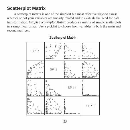
Scatterplot MatrixA scatterplot matrix is one of the simplest but most effective ways to assess

whether or not your variables are linearly related and to evaluate the need for data transformation. Graph | Scatterplot Matrix produces a matrix of simple scatterplots in a simplifi ed format. Use a picklist to choose from variables in both the main and second matrices.

26

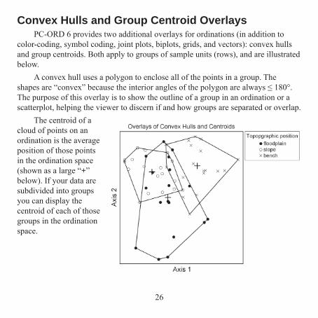
Convex Hulls and Group Centroid OverlaysPC-ORD 6 provides two additional overlays for ordinations (in addition to

color-coding, symbol coding, joint plots, biplots, grids, and vectors): convex hulls and group centroids. Both apply to groups of sample units (rows), and are illustrated below.

A convex hull uses a polygon to enclose all of the points in a group. The shapes are “convex” because the interior angles of the polygon are always ≤ 180°. The purpose of this overlay is to show the outline of a group in an ordination or a scatterplot, helping the viewer to discern if and how groups are separated or overlap.

The centroid of a cloud of points on an ordination is the average position of those points in the ordination space (shown as a large “+” below). If your data are subdivided into groups you can display the centroid of each of those groups in the ordination space.

27

A Decision Tree for BeginnersPC-ORD includes a decision tree (Advisor | Wizard) to help you decide how to

analyze your data. You can also use the wizard as a self teaching tool. We attempt to deal only with relatively common data analysis problems that you are likely to encounter with ecological community data. In practice, many data sets have peculiarities or complexities that do not fi t well into this decision tree. Strive for understanding and experience beyond what is captured in the decision tree. Think creatively about the best approach to your particular question and data. Remember to think beyond the range of tools included in the decision tree, for example, “is this question best answered with a univariate method?” or “Is this problem best suited to a habitat model, where we have a single species response variable in relationship to multiple predictors?” Most simple univariate problems can be adequately addressed with the major statistical software packages. For habitat modeling, consider HyperNiche (see www.hyperniche.com), particularly if you like the interface in PC-ORD and our emphasis on tools that deal well with nonlinear responses along ecological gradients and interactions among ecological factors.

The decision tree consists of a set of nodes, all connected to a starting point, the root node. Your answers to questions about the purpose of the analysis or the nature of the data link a node to other nodes.

Nodes are of two kinds, Question-Answer nodes, and Conclusion-Action nodes. Question-Answer nodes navigate you through the tree. Conclusion-Action nodes are endpoints on the tree. Conclusion-Action nodes state the conclusion, followed by one or more actions: an option to run an analysis, a suggestion for an analysis (which may or may not be part of PC-ORD), or some other recommendation.

28

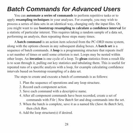
Batch Commands for Advanced UsersYou can automate a series of commands to perform repetitive tasks or to

apply resampling techniques in your analyses. For example, you may wish to process a series of data sets in an identical way, changing only the input fi les. Or, you might want to use bootstrap resampling to calculate a confi dence interval for a statistic of particular interest. This requires taking a random sample of a data set, performing an analysis, then repeating those steps many times.

A batch command is an action item selected from the PC-ORD menu system, along with the options chosen in any subsequent dialog boxes. A batch set is a sequence of batch commands. A loop is a programming structure that repeats itself a set number of times or until some criterion is met. Loops may be nested within other loops. An iteration is one cycle of a loop. To glean statistics from a result fi le is to scan through it, pulling out key statistics and tabulating them. This is useful for repeated runs of a specifi c analysis with a loop, for example calculating confi dence intervals based on bootstrap resampling of a data set.

The steps to create and execute a batch of commands is as follows:

1. Plan the sequence of operations and any loop structure.2. Record each component action.3. Save each command with a descriptive name.4. After all component commands have been recorded, create a set of

commands with File | New Batch Set and drag commands into the set.5. When the batch is complete, save it as a named fi le (Save As Batch Set),

then click Run.6. Add the loop structure(s) if desired.