Monetary policy and herd behavior in new-tech investment∗

Olivier Loisel†, Aude Pommeret‡and Franck Portier§

February 2008

Abstract

This paper studies the interaction between monetary policy and asset prices using a simple gen-eral equilibrium model in which asset-price bubbles may form due to herd behavior in investmentin a new technology whose productivity is uncertain. The economy is populated with one infinitelylived representative household and overlapping generations of finitely lived entrepreneurs. Entre-preneurs receive private signals about the productivity of the new technology and borrow fromthe household to publicly invest in the old or the new technology. Monetary policy intervention,by affecting the cost of resources for entrepreneurs, can make the entrepreneurs invest in the newtechnology if and only if they have received a favourable private signal. In doing so, it reveals thissignal and hence prevents herd behavior and the asset-price bubble. We identify conditions underwhich such a monetary policy intervention is socially desirable.

Key Words : Monetary Policy — Asset Prices — Informational Cascades.

JEL Classification : E52, E32

1 Introduction

Should monetary policy react to perceived asset-price bubbles over and above their short-term effects

on the business cycle? This old question has been hotly debated again since the remarkable rise

and fall in new-tech equity prices in developed economies in the late 1990s and early 2000s. Today’s

conventional answer among central bankers is "no". This answer stems from the consideration of the

following trade-off. On the one hand, if there is actually a bubble, then such a monetary policy reaction

may reduce its size and/or its duration, and hence its welfare costs due to overinvestment in the short

to medium term (when the bubble grows) and macroeconomic volatility in the medium term (when the

bubble bursts). On the other hand, if alternatively there is actually no bubble, then such a monetary

∗We thank Anne Épaulard and Sujit Kapadia for their comments. Part of this work was done when Franck Portierwas visiting scholar at the Banque de France, under a program organized by the Fondation de la Banque de France,whose financial support is gratefully acknowledged.

†Banque de France and Cepremap. The views expressed in this paper are those of the authors and should not beinterpreted as reflecting those of the Banque de France.

‡Université de Savoie and Université de Lausanne.§Toulouse School of Economics.

1

policy reaction will reduce welfare in the short term. Given this trade-off, such a monetary policy

reaction can be viewed as an insurance-against-bubbles policy, and the conditions most commonly

stressed by central bankers for its desirability are the following ones: i) the central bank should be

sufficiently certain that there is actually a bubble; ii) the cost of reacting as the bubble grows should

be low enough, in particular the bubble should be sufficiently sensitive to modest interest-rate hikes;

iii) the cost of reacting only when the bubble bursts, or not reacting at all, should be high enough.

Because they commonly view these conditions as unlikely to be met in practice (Greenspan, 2002;

Bernanke, 2002; Trichet, 2005; Rudebusch, 2005; Kohn, 2006; Mishkin, 2007), central bankers thus

usually conclude that, in most if not all cases, such a monetary policy reaction is not desirable1.

This paper seeks to challenge this view by considering a simple general-equilibrium model in which,

because asset-price bubbles are modeled as (rational) herd behavior, these three conditions can easily

be met. We focus on bubbles in new-tech equity prices, as our argument rests on some productivity

considerations that are not likely to play a key role in the development of other kinds of asset-price

bubbles, e.g. bubbles in house prices. More precisely, we assume that a new technology becomes

available whose productivity will be known with certainty only in the medium term. Entrepreneurs

sequentially choose whether to invest in the old or the new technology, each of them on the basis

of both the previous investment decisions that she observes and a private signal that she receives

about the productivity of the new technology. Herd behavior may then arise as the result of an

informational cascade (Banerjee, 1992; Bikhchandani, Hirshleifer and Welch, 1992) that corresponds

to a situation in which, because the first entrepreneurs choose to invest in the new technology as

they receive encouraging private signals about its productivity, the following entrepreneurs rationally

choose to invest in the new technology too whatever their own private signal.

In this context, monetary policy tightening, by making borrowing dearer for the entrepreneurs,

can make them invest in the new technology if and only if they receive an encouraging private signal

1Trichet (2005) however points out that, should all three conditions be met at some occasion, its monetary analysiswould probably enable the European Central Bank to react to the medium- to long-term effects of the perceived asset-price bubble on the business cycle without departing from the current framework of its monetary policy strategy.

2

about its productivity. In doing so, it prevents herd behavior and hence the bubble in new-tech

equity prices. Under this new explanation of bubbles in new-tech equity prices, the three conditions

mentioned above can be met: i) the central bank can detect herd behavior with certainty, even though

it then knows less about the productivity of the new technology than each entrepreneur; ii) given the

fragility of informational cascades, a modest monetary policy intervention can be enough to interrupt

herd behavior, even though it may not interrupt the new-tech investment craze2; iii) as we show,

under certain conditions, such a monetary policy intervention is ex ante preferable, in terms of social

welfare, to the laisser-faire policy (itself always preferable to the policy of reacting only when the

bubble bursts).

This paper is closely related to a large body of literature on whether the monetary policy rule

should make the current short-term nominal interest rate react to some measure of asset-price or credit

developments, in addition to standard variables (such as the current or expected future inflation rate,

the current output gap and the past short-term nominal interest rate), during an asset-price boom

that may correspond to an asset-price bubble. This literature has not reached a consensus on the

answer to that question. Indeed, on the one hand, Bernanke and Gertler (1999, 2001) and Gilchrist

and Leahy (2002) find that there is no need to include past asset prices in the monetary policy rule,

essentially because inflation and asset prices move jointly in their models. Similarly, Tetlow (2006)

obtains that, except in particular cases, there is no need to include current asset-price growth in the

monetary policy rule. On the other hand, Cecchetti, Genberg, Lipsky and Wadhwani (2000) find

that, if the central bank knows the size of the asset-price misalignment (admittedly a big “if”), then

it should add the past asset-price misalignment in its monetary policy rule. Moreover, Gilchrist and

Saito (2006) obtain that, even when the central bank has no clue about the size of the asset-price

misalignement, it is worth adding current asset-price growth in the monetary policy rule, in essence

because asset-price growth reflects distortions in the resource allocation more closely than inflation in

2The latter outcome would be expected by many a central banker, e.g. Greenspan (2002), Bernanke (2002) and Kohn(2006).

3

their model. Finally, Christiano, Ilut, Motto and Rostagno (2007) find that it is worth adding credit

growth in the monetary policy rule because, contrary to inflation, credit growth increases during the

asset-price boom in their model.

Our way of modeling bubbles in new-tech equity prices has some important advantages over each of

the following three ways in which this literature models asset-price bubbles. First, it may be modeled as

an exogenous boom-and-bust term in the asset-price-dynamics equation (Bernanke and Gertler, 1999,

2001; Cecchetti, Genberg, Lipsky and Wadhwani, 2000; Tetlow, 2006). This ad hoc modeling makes

the bubble by construction insensitive to monetary policy, and tends to cast doubt on the relevance

of the welfare function considered. By contrast, our modeling makes the bubble sensitive to monetary

policy, and enables us to use a micro-founded welfare function. Second, the asset-price bubble may

be modeled as the result of favourable public news about future productivity that eventually fails to

materialize (Gilchrist and Leahy, 2002; Christiano, Ilut, Motto and Rostagno, 2007). In this context,

given that expectations are assumed to be rational and that the central bank is assumed to have no

informational advantage over the private sector and therefore to be as much surprised by the lower-

than-expected eventual productivity level as the private sector, a proper unconditional assessment of

the desirability of a given monetary policy requires to consider not only the case where the favourable

news does not materialize, but also the case where it does, and to assign an occurrence probability

to each case − something this branch of the literature usually does not do3. Modeling the asset-

price bubble as herd behavior enables us to do just that in a micro-founded way. Third and finally,

the asset-price bubble may be modeled as the result of a permanent increase in productivity growth

that economic agents gradually recognize afterwards (Gilchrist and Saito, 2006). However, in our

new-technology context, this late-recognition assumption may be viewed as less relevant than the

early-news assumption that we make.

The other side of the coin, though, is that our way of modeling bubbles in new-tech equity prices

3Gilchrist and Leahy (2002) do actually consider both cases, without needing to assign an occurrence probability toeach of them, because the “strong inflation-targeting” monetary policy that they consider is very close to the optimalmonetary policy in both cases.

4

and our wish to secure some analytical results compel us to consider a highly stylised model that

fails to reproduce some basic characteristics of observed new-tech investment crazes, most notably the

concomitant steady growth in consumption and asset prices. Indeed, this model predicts that, during

a new-tech investment craze, as long as some uncertainty remains about the productivity of the new

technology, consumption should initially jump to a lower level and remain at this level thereafter,

while asset prices should initially jump to a higher level and, under the laisser-faire policy, remain

at that level thereafter. We therefore view our paper as a first step in building an empirically more

relevant model of herd behavior in new-tech investment4.

Our paper is also related to the literature on the role of informational cascades in the business

cycle. Within this literature, the paper closest to ours is that of Chamley and Gale (1994), which

models investment collapses as the result of herd behavior. A first difference between the two papers is

that we consider a general-equilibrium model, which enables us to conduct policy analysis, while they

consider a partial-equilibrium model. A second difference is that they consider an endogenous timing

of investment decisions, as they are also interested in modelling strategic investment delay, while we

consider an exogenous timing of investment decisions. And a third difference is that, in equilibrium,

in their model, although an investment collapse may be socially non-optimal, an investment surge is

always socially optimal, while in ours, both new-tech and old-tech investment crazes may be socially

non-optimal.

The remainder of the paper is structured as follows. Section 2 presents the model. The compet-

itive equilibrium with public information about the productivity of the new technology is described

in section 3. We introduce private information, derive the results about the desirability of policy

intervention in a simple case and conduct simulations in more complex cases in section 4. Section 5

concludes.4This research agenda would undoubtedly benefit from the works of Beaudry and Portier (2004), Jaimovich and

Rebelo (2006) and Christiano, Ilut, Motto and Rostagno (2007), whose models predict an increase in aggregate output,employment, investment and consumption in response to news of future technological improvement.

5

2 The model

We consider an economy populated with infinitely lived households, overlapping generations of finitely

lived entrepreneurs, and a central bank. For simplicity, we limit our analysis to outcomes symmetric

across entrepreneurs and across households, i.e. there is one representative household and, in each

generation, one representative entrepreneur. Time is discrete and there is a single good that is non-

storable and can be consumed or invested.

2.1 Technology

A production project requires κt units of good in period t, the investment period, and delivers Yt+N =At+NLαt+N units of good in period t + N , where At+N is a productivity parameter, Lt+N is labor

services and 0 < α < 1.At a given period t, different technologies might be available. A technology z ∈ R is defined by a

period t investment cost κt = κ(z) and by a period t+N productivity parameter At+N = A(z). Ft is

the set of technologies available at period t, which includes the particular case z = 0 corresponding tothe absence of any production project, with κ(0) = 0 and A(0) = 0.

A production project needs a newborn entrepreneur to be undertaken, and an entrepreneur cannot

undertake more than one project at the same time.

2.2 Preferences

The representative household supplies inelastically one unit of labor per period, and her preferences

are represented by the following utility function:

Ut = EΩ(h,t)∞∑

j=0βj ln(ct+j)

where Ω(h, t) is her information set at date t, ct her consumption at date t, and β ∈ (0, 1). We choosea logarithmic utility to simplify the algebra.

At each date, one representative entrepreneur is born, and lives for N + 1 periods. She consumes

only in her last period of life and has linear preferences. The utility of an entrepreneur born at date

6

t is given by:Vt = βNEΩ(e,t)cet+N

where Ω(e, t) is her information set and cet her consumption at date t. We assume that each generationcontains a large number of entrepreneurs, so that the representative entrepreneur is price-taker.

2.3 Market organization

We present here the real economy under Laissez-Faire. We will later introduce public intervention,

which will receive an interpretation as monetary policy. All markets (good, labor, bonds) are compet-

itive. The final good is the numéraire. A newborn entrepreneur may want to borrow κ to undertake aproduction project. The return from this investment will be the profit she will obtain from production

N periods onwards. We assume that the only financial market that is opened is a market for N -periodbonds. Both the household and the entrepreneurs have access to this market, and there is secondary

market for those bonds. We denote Bt+N the number of bonds that pay in period t+N , and that hasbeen subscribed by the household in period t. Each of this bond will pay one unit of good in periodt+N , and its price is denoted qt. Bet is the number of bonds emitted by the entrepreneurs.

2.4 Resource constraints

The resource constraint on the good market states that the total number of goods consumed and

invested cannot be larger than the total amount of goods available in a given period. Let zt ∈ Ft

denote the technology chosen by the entrepreneur at date t. We have:

ct + cet + κ(zt) ≤ Yt

Labor services cannot exceed the total amount of labor that is supplied, so that

Lt ≤ 1

2.5 Agents programs

The household enters period t with a portfolio St−1 = (Bt, ..., Bt+n, ...., Bt+N−1) of bonds, that pay

interest if at maturity. The household then decides how much to consume and how much to save,

7

supplying inelastically one unit of labor. The household program can be recursively written in the

following way:

W (St−1) = maxct,Bt+N

ln(ct) + βEΩ(h,t)W (St)

subject to ct + qtBt+N ≤ Bt +wtLstLst = 1

,

where wt is the wage rate at date t. The houshold’s optimality conditions can be reduced to

qt = βNEΩ(h,t)[ ctct+N

],

Lst = 1,

and a transversality condition.

Let us now consider the optimal behavior of the representative newborn entrepreneur of period t.She borrows κ(zt) in period t, hires Lt+N and produces Yt+N in period t + N . Note that zt = 0 is

a possible option, which corresponds to no investment in t and no production in t +N . Productionproceeds are used to pay wages, reimburse the debt and to consume. Budget constraints of an active

entrepreneur born in period t are therefore

κ(zt) ≤ qtBet+N ,ct+N +Bet+N ≤ Πt+N = A(zt)Lαt+N − wt+NLt+N .

Labor demand L will be set such that marginal productivity of labor equalizes the real wage w:

wt+N = αA(zt)Lα−1t+N .

Therefore, the intertemporal utility of a new-born entrepreneur is

V = maxzt∈FtV e(zt) = maxzt∈FtβNEΩ(e,t)(Πt+N −

1

qtκ(zt)).

2.6 Competitive equilibrium

In this economy, a competitive equilibrium is a sequence of prices qt, wt and quantities Bt, Bet , ct, cet , Lt

∀ t ≥ 1 such that, given initial conditions and for an exogenous sequence of technological possibili-

ties Ft, (i) household’s consumption and bonds holding solve her maximization problem given prices,

8

(ii) investment decision zt maximizes expected intertemporal utility of newborn entrepreneurs givenprices, (iii) labor demand Lt maximizes aged N + 1 entrepreneurs profits given prices and (iv) labor,

bonds and good markets clear.

2.7 Discussion

In the set of assumptions that we have made, some are needed for the analytical tractability of the

model, while some are less restrictive than what they look. First, we consider risk-neutral entrepreneurs

that consume only in the last period of their life. This assumption is crucial in order to solve the

model when we introduce private information and potential informational cascades. Second, we have

introduced bonds of maturity N only. This is not a restriction since other maturity bonds would not

be traded. Third, we assume that only non-contingent debt contracts are possible. This assumption

is a priori restrictive because, when we introduce entrepreneurs’ private signals, households might

prefer to propose contingent debt contracts to entrepreneurs in order to gain some information about

their private signal. That would complicate the analysis since the desirability of a monetary policy

intervention would then depend on the social cost of these contingent debt contracts. Fourth, we

consider investment projects that pay only N periods ahead. This assumption will be crucial when

we introduce private signals and the possibility of informational cascades.

3 Competitive equilibrium with public information

In this section, we consider economies with public information only. In tranquil times, there is only

one technology available, and we study the existence, uniqueness and stability of the steady state. We

then introduce technological change: a new technology is available today, that will happen to be more

productive or not N periods onwards. We study the properties of the equilibrium path in such a case.

The results that we obtain will be useful for the analysis of the private-information case.

9

3.1 Tranquil times

We assume that, in tranquil times, only one technology is available (∀t ∈ Z, Ft = 0, z). We alsoassume that there exists c > 0 such that there exists an equilibrium at which ∀t ∈ Z, zt = z andct = c. A necessary and sufficient condition for that is

βN (1− α)A (z)− κ (z) > 0 (1)

and αA (z)− κ (z) + β−Nκ (z) > 0. (2)

Indeed, if ∀t ∈ Z, ct = c, then ∀t ∈ Z, qt = βN ≡ q, i.e. the N -period interest factor is Rt = q−1 =β−N ≡ R. If, moreover, ∀t ∈ Z, zt = z, then the labor market equilibrium condition implies ∀t ∈ Z,wtLt = αA (z) and Πt = (1− α)A (z), from which we deduce c = αA (z)− κ (z) + β−Nκ (z), which isstrictly positive if and only if (2) holds. And entrepreneurs are active if and only if V (z) > V (0), thatis to say if and only if (1) holds.

Note that, under conditions (1) and (2), this steady-state equilibrium is stable in the sense that

if ∀t ∈ Z−, zt = z, ct = c and qt = q, then there exists a unique equilibrium at which ∀t ∈ N∗,zt = z, ct = c and qt = q. Indeed, suppose that ∀t ∈ Z−, zt = z, ct = c and qt = q. If there existedt ∈ 1, ..., N such that zt = 0, then we would get ct+N = 0. But since ct > 0 due to (2), that wouldimply qt −→ +∞ and hence zt = z, which would be contradictory. Therefore, ∀t ∈ 1, ..., N, zt = z,ct = c and qt = q, and by recurrence we easily obtain that ∀t ∈ N∗, zt = z, ct = c and qt = q.

We also assume that this steady-state equilibrium is locally dynamically stable in the sense that

there exist some neighborhoods Nc of c and Nq of q such that if ∀t ∈ Z−, zt = z, ct ∈ Nc and qt ∈ Nq,

then there exists an equilibrium at which ∀t ∈ N∗, zt = z, ct ∈ Nc, qt ∈ Nq and (ct, qt) −→ (c, q) ast −→ +∞. A necessary and sufficient condition for that is

βN > κ (z)|αA (z)− κ (z)| . (3)

Indeed, if ∀t ∈ Z, zt = z, then ∀t ∈ Z,

qt = βN αA (z)− κ (z) + κ(z)qt−N

αA (z)− κ (z) + κ(z)qt

10

and hence

qt − βN = −κ (z)αA (z)− κ (z)

qt−N − βN

qt−N ,

so that any sequence (qt)t∈Z originating in the neighborhood of q will converge towards q if and onlyif (3) holds.

3.2 Technological change

We now consider the response of the economy to the unexpected availability of a new technology. We

assume that the economy is at its steady state until date 0 included (∀t ∈ Z− and ∀k ∈ N, Ft = 0, z,Et (Ft+k) = 0, z, zt = z, ct = c and qt = q) and that a new technology z > z becomes available fromdate 1 onwards (∀t ∈ N∗ and ∀k ∈ N, Ft = 0, z, z and Et (Ft+k) = 0, z, z). This new technologyrequires more investment than the old one: κ (z) > κ (z). It may be “good” and lead N periods later

to a productivity parameter A (z) > A (z), or it may be “bad” and lead N periods later to the same

productivity parameter A (z) as the old technology z: in words, entrepreneurs invest more to raiselabour productivity, but labour productivity remains unchanged. We note p the probability that thenew technology is good and assume that this probability is common knowledge at dates 1 to N . Wealso assume that whether the new technology is good or bad becomes common knowledge at date

N + 1 even if there has been no investment in the new technology at date 1.

At each date t ∈ N∗, the representative newborn entrepreneur chooses zt ∈ 0, z, z and borrowsq−1t κ (zt). The representative entrepreneurs born at dates− (N − 1) to 0 pay back their debts at dates 1

to N at the interest factor R. Therefore, ∀t ∈ 1, ..., N, the sequence of the representative household’sconsumption is ct = αA (z) − κ (zt) + β−Nκ (z). We restrict our analysis to equilibria at which

∀t > N , zt = z if the new technology turns out to be good and zt = z otherwise. As a consequence,we have: ∀t > N , ct = αA (z) − κ (z) + q−1t−Nκ (z) if zt−N = z and the new technology is good,

ct = αA (z)−κ (z)+q−1t−Nκ (z) if zt−N = z and the new technology is bad, ct = αA (z)−κ (z)+q−1t−Nκ (z)if zt−N = z and the new technology is good, and ct = αA (z)− κ (z) + q−1t−Nκ (z) if zt−N = z and thenew technology is bad.

11

We focus on the real-interest-rate transmission channel of monetary policy, i.e. monetary policy

has an exoect on the economy only through its effect on the real interest rate. Technically speaking,

this can be done by modeling monetary policy as a tax (or subsidy) on lending together with a

positive (or negative) lump-sum transfer to the representative household. More precisely, at date t therepresentative household lends qtBt+N to the entrepreneur and gives (τ t − 1) qtBt+N to the central

bank (when τ t > 1) or receives − (τ t − 1) qtBt+N from the central bank (when 0 < τ t < 1), while thecentral bank gives a lump-sum transfer Tt ≡ (τ t − 1) qtBt+N to the representative household (when

τ t > 1) or receives a lump-sum transfer Tt ≡ − (τ t − 1) qtBt+N from the representative household

(when 0 < τ t < 1). The intertemporal budget constraint of the representative household thus becomesat date t

ct + τ tqtBt+N ≤ Bt + wtLt + Tt.

This implies

τ tqt = βNEΩ(h,t)[ ctct+N

].

In particular, for t ∈ 1, ..., N, when zt = z, we get

τ tqt = βN[αA (z)− κ (z) + κ (z)

βN

] pαA (z)− κ (z) + κ(z)

qt+

1− pαA (z)− κ (z) + κ(z)

qt

. (4)

Noting

∀x ≥ z, τu (x) ≡ βN [αA (z)− κ (x)] + κ (z)κ (x) ,

we obtain the following proposition concerning qt for t ∈ 1, ..., N when zt = z:

Proposition 1: i) there exists a strictly positive real number qt solution of (4) for all p ∈ [0; 1] ifand only if αA (z)− κ (z) > 0 and τ t < τu (z); ii) then qt, which we note q (z, τ t, p, 0), is unique, and∂q(z,τ t,p,0)

∂τ t < 0 and ∂q(z,τ t,p,0)∂p > 0.

Proof : cf appendix A.

12

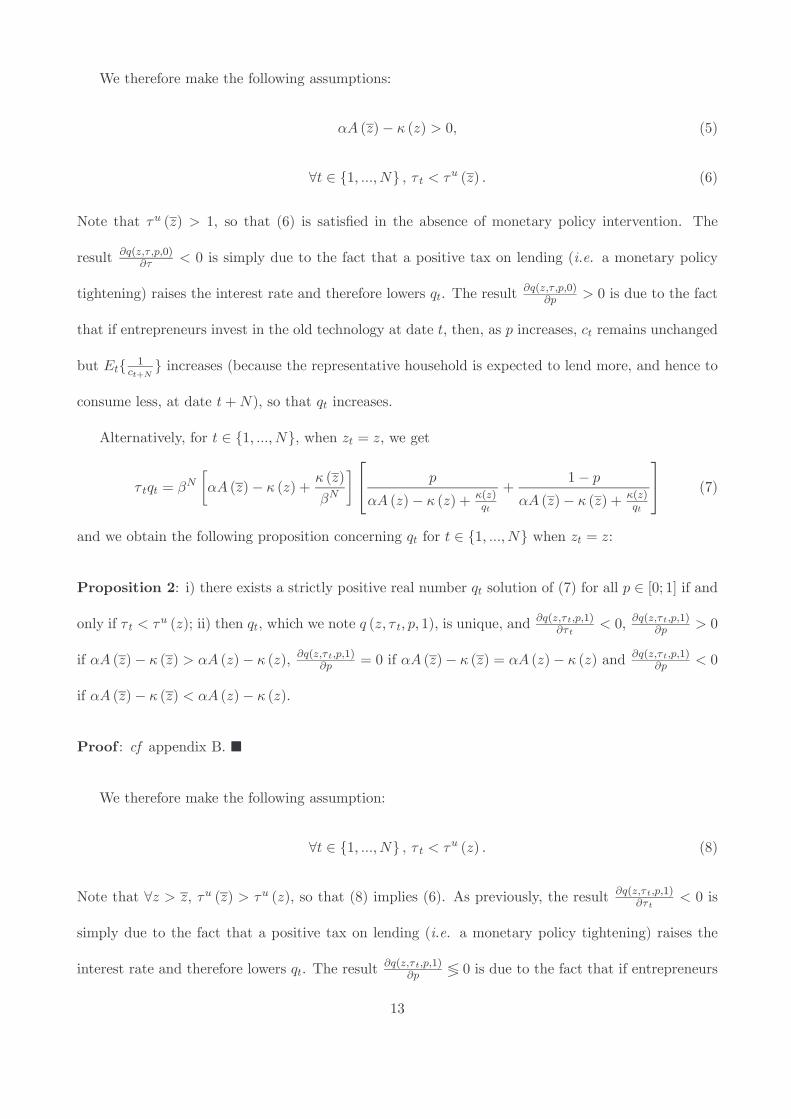
We therefore make the following assumptions:

αA (z)− κ (z) > 0, (5)

∀t ∈ 1, ..., N , τ t < τu (z) . (6)

Note that τu (z) > 1, so that (6) is satisfied in the absence of monetary policy intervention. The

result ∂q(z,τ ,p,0)∂τ < 0 is simply due to the fact that a positive tax on lending (i.e. a monetary policy

tightening) raises the interest rate and therefore lowers qt. The result ∂q(z,τ ,p,0)∂p > 0 is due to the fact

that if entrepreneurs invest in the old technology at date t, then, as p increases, ct remains unchangedbut Et 1

ct+N increases (because the representative household is expected to lend more, and hence to

consume less, at date t+N), so that qt increases.Alternatively, for t ∈ 1, ..., N, when zt = z, we get

τ tqt = βN[αA (z)− κ (z) + κ (z)

βN

] pαA (z)− κ (z) + κ(z)

qt+

1− pαA (z)− κ (z) + κ(z)

qt

(7)

and we obtain the following proposition concerning qt for t ∈ 1, ..., N when zt = z:

Proposition 2: i) there exists a strictly positive real number qt solution of (7) for all p ∈ [0; 1] if andonly if τ t < τu (z); ii) then qt, which we note q (z, τ t, p, 1), is unique, and ∂q(z,τ t,p,1)

∂τ t < 0, ∂q(z,τ t,p,1)∂p > 0

if αA (z)− κ (z) > αA (z)− κ (z), ∂q(z,τ t,p,1)∂p = 0 if αA (z)− κ (z) = αA (z)− κ (z) and ∂q(z,τ t,p,1)

∂p < 0if αA (z)− κ (z) < αA (z)− κ (z).

Proof : cf appendix B.

We therefore make the following assumption:

∀t ∈ 1, ..., N , τ t < τu (z) . (8)

Note that ∀z > z, τu (z) > τu (z), so that (8) implies (6). As previously, the result ∂q(z,τ t,p,1)∂τ t < 0 is

simply due to the fact that a positive tax on lending (i.e. a monetary policy tightening) raises the

interest rate and therefore lowers qt. The result ∂q(z,τ t,p,1)∂p ≶ 0 is due to the fact that if entrepreneurs

13

invest in the new technology at date t, then, as p increases, ct remains unchanged but Et 1ct+N

either increases or decreases depending on the sign of [αA (z)− αA (z)]− [κ (z)− κ (z)] (because therepresentative household is expected both to lend more, as κ (z) > κ (z), and to receive a higher wage,as αA (z) > αA (z), at date t+N), so that qt either increases or decreases depending on the sign of[αA (z)− αA (z)]− [κ (z)− κ (z)].

Assuming that ∀t > N , τ t = 1 (this assumption will be justified in the next section), we also

obtain the following proposition concerning qt for t > N :

Proposition 3: qt is unique and strictly positive for all t > N and all p ∈ [0; 1], and limt−→+∞qt = βN

for all p ∈ [0; 1], if and only if conditions (17), (18), (19) and (20) are satisfied.

Proof: cf appendix C.

We therefore assume that parameters are such that (17), (18), (19) and (20) hold. Note that, given

(5), this implies that ct is unique and strictly positive for all t > N and all p ∈ [0; 1].Finally, noting τ l (z) ≡ 0 if A (z)κ (z) ≥ A (z)κ (z) and

τ l (z) ≡ κ (z) [κ (z)− κ (z)]− [αA (z)− αA (z)] [κ (z) (1− βN)+ αA (z)βN]

αA (z)κ (z)− αA (z)κ (z)

if, alternatively, A (z)κ (z) < A (z)κ (z), we obtain the following proposition:

Proposition 4: q (z, τ , p, 0) > q (z, τ , p′, 1) for all (p, p′) ∈ [0; 1]2 if and only if τ > τ l (z).

Proof : cf appendix D.

We make the following assumption:

∀t ∈ 1, ..., N , τ t > τ l (z) , (9)

so that we get ∀ (p, p′) ∈ [0; 1]2, q (z, τ , p, 0) > q (z, τ , p′, 1), which will simplify the analysis in thefollowing section. In words, that means that the interest rate maximized over p ∈ [0; 1] that prevails

14

when the entrepreneurs borrow little (as they invest in the old technology) is strictly lower than the

interest rate minimized over p ∈ [0; 1] that prevails when the entrepreneurs borrow much (as they

invest in the new technology). Note that ∀z > z, τ l (z) < 1, so that (9) is satisfied in the absence ofmonetary policy intervention.

4 Competitive equilibrium with private information

We assume that the economy is initially at the steady state with a technology z. Therefore, theinvestment cost and the interest rate are respectively: κ−i = κ (z) and q−i = βN for i ≥ 0. Also

recall that for simplicity we limit our analysis to outcomes symmetric across entrepreneurs and across

households i.e. there is one representative household and, in each generation, one representative

entrepreneur.

4.1 General case

Information accumulation is modelled as follows:

• The representative entrepreneur starts period t with the public information available at timet − 1. Public information is derived from the observation of the investment behavior of the

previous representative entrepreneurs. We note µt−1 the probability that the new technology isgood based on public information available at date t− 1. µt−1 is therefore the prior at time t.

• At time t, the representative entrepreneur receives a private signal St. This signal can be eithergood, then St = 1, or bad, then St = 0. This signal is then incorporated into the private

information available for the representative entrepreneur at time t. We note µt the probabilitythat the new technology is good based on private information available at date t, which includesSt if t > 0. µt is therefore the posterior at time t. Let λ denote the probability that a signal,whether good or bad, is right. According to Bayes’ theorem:

µt = St µt−1λµt−1λ+

(1− µt−1

)(1− λ) + (1− St) µt−1 (1− λ)

µt−1 (1− λ) + (1− µt−1)λ

15

Moreover, let us note µ0t the value taken by µt when St = 0 and µ1t the value taken by µt whenSt = 1 for t ∈ 1, ..., N.

• Still at time t, investment decision It is taken. If the representative investor invests in the newtechnology then we note It = 1; if she invests the old technology, It = 0. This decision is publicinformation that is available at time t. Therefore, the probability that the new technology is

good based on public information available at date t, which we note µt includes It if t > 0.

According to this information structure, the interest rate becomes: qt = q (z, τ t, µt, It).

Noting p0 ≡ µ0,

pi ≡ pi−1λpi−1λ+ (1− pi−1) (1− λ) and p−i ≡ p−i+1 (1− λ)

p−i+1 (1− λ) + (1− p−i+1)λ for i ∈ N∗,

B (z) ≡ κ (z)− κ (z)(1− α) [A (z)−A (z)] for z > z and B (z) ≡

dκdz∣∣z=z

(1− α) dAdz∣∣z=z

,

we obtain the following proposition:

Proposition 5: in equilibrium, ∀t ∈ 1, ...,N, there are only three possibilities, and these possibilitiesare mutually exclusive: i) either µ1t q

(z, τ t, µt−1, 0) < B (z), then It = 0 whatever St ∈ 0, 1 and

µt = µt−1; ii) or µ0t q(z, τ t, µt−1, 1

) > B (z), then It = 1 whatever St ∈ 0, 1 and µt = µt−1; iii) orµ0t q

(z, τ t, µ0t , 0) < B (z) and µ1t q

(z, τ t, µ1t , 1) > B (z), then It = St whatever St ∈ 0, 1 and µt = µt.

Proof : cf appendix E.

This implies in particular that ∀t ∈ 1, ..., N, ∃i ∈ Z, µt = pi and µt ∈ pi−1, pi, pi+1.Note that we can rewrite the necessary and sufficient condition for the monetary policy intervention

to ensure the absence of cascade at date t in an alternative way. Indeed, from (4) and (7), it is easy to

see that, whatever z ≥ z, p ∈ [0; 1] and Q > 0, there exists a unique τ > 0 such that q (z, τ , p, 0) = Qand there exists a unique τ > 0 such that q (z, τ , p, 1) = Q. Let us note

τ l∗ (z, p) ≡ βN[αA (z)− κ (z) + κ (z)

βN

] p[αA (z)− κ (z)] B(z)p + κ (z) +

1− p[αA (z)− κ (z)] B(z)p + κ (z)

16

the unique value of τ such that q (z, τ , p, 0) = B(z)p and

τu∗ (z, p) ≡ βN[αA (z)− κ (z) + κ (z)

βN

] p[αA (z)− κ (z)] B(z)p + κ (z) +

1− p[αA (z)− κ (z)] B(z)p + κ (z)

the unique value of τ such that q (z, τ , p, 1) = B(z)p . Since ∂q(z,τ ,p,0)

∂τ < 0 and ∂q(z,τ ,p,1)∂τ < 0 (as stated

in propositions 1 and 2), the necessary and sufficient condition for the monetary policy intervention

to ensure the absence of cascade at date t can therefore be rewritten τ l∗ (z, µ0t) < τ t < τu∗ (z, µ1t

).

In order to illustrate the mechanism of monetary policy intervention, suppose for a moment that

there exists t ∈ 1, ..., N at which there is an upward cascade under laisser-faire, i.e. that thereexists t ∈ 1, ..., N such that µ0t q

(z, 1, µt−1, 1) > B (z). Then, as a direct application of proposition

5, a necessary condition for the monetary policy intervention to interrupt the cascade at date t isµ0t q

(z, τ t, µ0t , 0) < B (z). Given proposition 4, µ0t q

(z, 1, µt−1, 1) > B (z) implies µ0t q

(z, 1, µ0t , 0) >

B (z). Since ∂q(z,τ ,p,0)∂τ < 0 (as stated in proposition 1), τ t > 1 is therefore a necessary condition for

the monetary policy intervention to interrupt the cascade at date t. In other words, monetary policymust be tightened to interrupt an upward cascade.

Lastly, two points are worth noting about monetary policy. First, our assumption that τ t = 1

for all t > N is not restrictive because, whatever happened until date N , there is no rationale forintervening after date N , as there is then no financial market imperfection anymore. Second, thereis no problem of time-inconsistency for monetary policy since ∀t ∈ 1, ...,N, the private agents’decisions at date t depend on τ t but not on Et τ t+k for k > 0.

4.2 A simple case

In order to focus on analytically tractable informational cascades, we assume here that N = 3 and zis arbitrarily close to z. This implies that ∀p ∈ [0; 1], ∀I ∈ 0, 1, q (z, 1, p, I) is arbitrarily close toq (z, 1, p, I) = β3. We also impose the following condition on the parameters which, given proposition5, is necessary for an arbitrarily small intervention to be enough to avoid the cascade with a prior p1:

dAdz∣∣∣∣z=z

=1

(1− α) p0β3dκdz∣∣∣∣z=z

. (10)

17

We also assume that, under laisser-faire (τ1 = τ2 = τ3 = 1), there is no cascade at t = 1 and a cascadeat t = 2 when S1 = 1. The necessary and sufficient condition for that is

β3[(1− α)β3p0 d2A

dz2∣∣∣z=z −

d2κdz2∣∣∣z=z

]

2( dκdz∣∣z=z

)2 > 1 + βN (1− p1) + α1−α

p1p0

αA (z)− κ (z) . (11)

Indeed, given proposition 5, there is no cascade at t = 1 and a cascade at t = 2 when S1 = 1 underlaisser-faire if and only if p−1q (z, 1, p−1, 0) < B (z), p1q (z, 1, p1, 1) > B (z) and p0q (z, 1, p1, 1) > B (z),that is to say, given proposition 4, if and only if p−1q (z, 1, p−1, 0) < B (z) and p0q (z, 1, p1, 1) > B (z).The first condition is satisfied since B (z) = p0β3, due to (10), and since q (z, 1, p−1, 0) is arbitrarilyclose to β3. The second condition is satisfied if and only if

p0 ∂q (z, 1, p1, 1)∂z∣∣∣∣z=z

> dBdz∣∣∣∣z=z

. (12)

At date t = 2, under laisser-faire (τ2 = 1), the derivation of (7) with respect to z, taken at pointz = z, and the use of (10) lead to

∂q (z, 1, p1, 1)∂z

∣∣∣∣z=z= −

[1 + βN (1− p1)]+ αp1

(1−α)p0αA (z)− κ (z)

dκdz∣∣∣∣z=z

.

Besides, using (10), we also get

dBdz∣∣∣∣z=z

=βNp0

[d2κdz2∣∣∣z=z − (1− α)βNp0 d2A

dz2∣∣∣z=z

]

2 dκdz∣∣z=z

. (13)

Using the last two results to rewrite (12) leads to condition (11).

We focus on the case where S1 = 1, which implies µ1 = µ1 = p1 (and, if τ2 = 1, µ2 = p1). Forsimplicity, we consider the possibility of intervention only at time t = 2 (τ1 = τ3 = 1)5, and we focuson the “minimal” intervention to avoid a cascade at date t = 2, that is to say, of all the values of

τ2 such that there is no cascade at time t = 2, the one closest to 1 or, equivalently here, of all the

values of dτ2dz∣∣∣z=z such that there is no cascade at time t = 2, the one closest to 0. Our objective is

5There is no rationale to intervene at date t = 1, since there is no cascade at that date, but there could be a rationale tointervene at date t = 3, even though making S3 public would not benefit future entrepreneurs (since the true productivityof the new technology is known at date t = 4 anyway): indeed, making S3 public could benefit the household.

18

to examine whether this particular intervention is welfare-improving, not to determine the optimal

monetary policy6. Since τ l∗ (z, p0) = 1 < τu∗ (z, p2), this “minimal” intervention isdτ2dz∣∣∣∣z=z

=∂τ l∗ (z, p0)

∂z∣∣∣∣z=z

which, using (13), leads to

dτ2dz∣∣∣∣z=z

=βN dκ

dz∣∣z=z

βN [αA (z)− κ (z)] + κ (z)

p0 −

[αA (z)− κ (z)][d2κdz2∣∣∣z=z − (1− α)βNp0 d2A

dz2∣∣∣z=z

]

2( dκdz∣∣z=z

)2

.

(14)

From proposition 5 we also get

dq (z, τ2 (z) , p0, 0)dz

∣∣∣∣z=z=1

p0dBdz∣∣∣∣z=z

=βN[d2κdz2∣∣∣z=z − (1− α)βNp0 d2A

dz2∣∣∣z=z

]

2 dκdz∣∣z=z

. (15)

Finally, the derivation of (7) at date t = 2 with respect to z, taken at point z = z, and the use of (14)lead to

dq (z, τ2 (z) , p2, 1)dz

∣∣∣∣z=z=

−dκdz∣∣∣∣z=z

1 + βN (1 + p0 − p2) + α

1−αp2p0

αA (z)− κ (z) +βN[(1− α)βNp0 d2A

dz2∣∣∣z=z −

d2κdz2∣∣∣z=z

]

2( dκdz∣∣z=z

)2

. (16)

In order to determine whether such an intervention increases welfare, we compare the welfare of

both investors and households under this intervention (superscript I) and under laisser-faire (super-

script LF). To consider social welfare, we also introduce weights applied to households and entrepre-

neurs such that aggregate utility corresponds to GDP in this linearized case. Let pA be the probabilityof receiving a signal S2 = 1, i.e. pA = p1λ+ (1− p1) (1− λ), and pB be the probability of receiving asignal S3 = 1 once having received S2 = 0, ie. pB = p0λ+ (1− p0) (1− λ).

In the case of laissez-faire (cf appendix F), we obtain:

κ (z) + β3 [αA (z)− κ (z)]β3

dULF1

dz∣∣∣∣z=z

+dV LF1

dz∣∣∣∣z=z

=dκdz∣∣z=z

1− β[ p1(1− α) p0 − 1 + β3 (1− p1)

]> 0,

6Note that this “minimal” intervention may not be the optimal intervention even among the set of interventions atdate t = 2. Indeed, we know that social welfare is maximal under laisser-faire in the fictitious situation of public (ratherthan private) signals; any arbitrarily small intervention reduces social welfare in this fictitious situation, i.e. there isa neighbourhood of laisser-faire within which increasing intervention decreases social welfare in this situation; but as zbecomes arbitrarily close to z the size of this neighbourhood may tend towards zero; hence our “minimal” intervention(not to mention interventions of greater size), which reveals the private signal, may fall outside this neighbourhood.

19

dULF1

dz∣∣∣∣z=z

> 0,

and we find that dV LF1dz∣∣∣z=z is positive for

p1p0 sufficiently large (as can be easily checked, using (1))

and negative for p0 sufficiently close to 1. How can we get dV LF1dz∣∣∣z=z < 0 though each entrepreneur

individually gains from investing in the new technology? There are three possible reasons: i) en-

trepreneurs investing at dates 1 to N do not internalize the possible costs (in terms of interest-rate

fluctuations) that their actions will impose on the following entrepreneurs; ii) entrepreneurs investing

at dates t > N do not internalize the possible costs (again, via the interest rate) that their actions

impose on the entrepreneurs investing at dates 1 to N ; iii) if there were only one entrepreneur pergeneration, then she would choose between borrowing little at a low rate or borrowing much at a high

rate, and might prefer to borrow little at a low rate; but there are many of them, so that each of

them, taking the interest rate as given, has either to choose between borrowing little or much at a

low rate, or to choose between borrowing little or much at a high rate; if in both cases she prefers to

borrow much, then the only stable symmetric equilibrium is that all entrepreneurs borrow much at a

high rate.

In the case of intervention (cf appendix G), we obtain:

κ (z) + β3 [αA (z)− κ (z)]β3

dU I1

dz∣∣∣∣z=z

+dV I1

dz∣∣∣∣z=z

=

[ p1(1− α) p0 − 1

]+

β31− βp1

[1

(1− α) p0 − 1]

+β (1 + β) pA[ p2(1− α) p0 − 1

]+ β2 (1− pA) pB

[ p1(1− α) p0 − 1

] dκdz∣∣∣∣z=z

> 0,

dU I1

dz∣∣∣∣z=z

> 0,

and we find again that dV I1dz∣∣∣z=z is positive if the ratio between the discounted sum of future probabilities

for the technology to be good (p1, pAp2, (1− pA) pBp1) and p0 is sufficiently large, and negative forp0 sufficiently close to 1. Reasons for having dV LF

1dz∣∣∣z=z < 0 are pretty much the same as under

laissez-faire.

20

Lastly, we compare laissez-faire and intervention by computing:

κ (z) + β3 [αA (z)− κ (z)]β3

( dU I1

dz∣∣∣∣z=z

−dULF

1

dz∣∣∣∣z=z

)+

( dV I1

dz∣∣∣∣z=z

−dV LF1

dz∣∣∣∣z=z

)=

β (1− pA)1− α

[β(p1p0 − 1

)pB − α [1 + β (1− pB)]

] dκdz∣∣∣∣z=z

,

dU I1

dz∣∣∣∣z=z

−dULF

1

dz∣∣∣∣z=z

=β3 dκ

dz∣∣z=z

κ (z) + β3 [αA (z)− κ (z)]1− pA(1− α)β

[pB (p1 − p0)

p0[αβ3 +

(1− β3)κ (z)

A (z)]

−1 + β (1− pB)

β[αβ3 + κ (z)

αA (z)[(1− α) + α (1− β3)]

]]+βp0κ (z)αA (z)

+βκ (z) [αA (z)− κ (z)]

2αA (z)

(1− α)β3p0 d2A

dz2∣∣∣z=z −

d2κdz2∣∣∣z=z( dκ

dz∣∣z=z

)2

,

dV I1

dz∣∣∣∣z=z

−dV LF1

dz∣∣∣∣z=z

=dκdz∣∣∣∣z=z

1− pA(1− α)β

[pB (p1 − p0)

p0[(1− α)β3 −

(1− β3)κ (z)

A (z)]

+1 + β (1− pB)

βκ (z)αA (z)

[(1− α) + α (1− β3)]

]−βp0κ (z)αA (z)

−βκ (z) [αA (z)− κ (z)]

2αA (z)

(1− α)β3p0 d2A

dz2∣∣∣z=z −

d2κdz2∣∣∣z=z( dκ

dz∣∣z=z

)2

.

The conditions imposed on the parameters are listed in appendix H. It is clear that there exist some

calibrations of the parameters satisfying all these conditions and such that p0 (the initial prior onthe success of the new technology) is arbitrarily close to zero, λ (the precision of private signals)is arbitrarily close to one, and α < β

1+β . The results above imply that, for these calibrations, the

monetary policy intervention considered increases social welfare. Of course, when p0 is low, so is theprobability that S1 = S2 = 1 and therefore so is the probability to intervene.

4.3 Numerical simulations

In this section we plan to run numerical simulations in order to rank different monetary policy in-

terventions according to welfare criteria for various calibrations satisfying the conditions listed in

appendix H (in the general case). We aim at numerically generalizing the analytical results obtained

in the previous subsection by relaxing the assumptions that N = 3, that z is arbitrarily close to z,that (10) holds and that monetary policy is limited to the “minimal” intervention to avoid a cascade

21

at date t = 2. On the one hand, we expect the relaxation of the assumption N = 3 to spread the gains

of the monetary policy intervention over more periods and therefore to increase the desirability of this

intervention, i.e. to make the conditions for its desirability less stringent. Moreover, the relaxation of

the assumption that z is arbitrarily close to z will make households’ risk-aversion matter in welfarecomputations and may therefore also be expected to increase the desirability of the monetary policy

intervention. On the other hand, the relaxation of the assumption that parameters are such that

the monetary policy intervention can be arbitrarily small will increase the distortion caused by this

intervention and will therefore tend to decrease its desirability. Sensitivity analyses will be carried out

for each parameter. Lastly, we will consider the case where the central bank does not observe µ0 andtherefore can neither identify a cascade with certainty nor know how much intervention exactly is

needed to prevent a cascade. This will amount to extend our work in a similar way as Bernanke and

Gertler (2001) extend on Bernanke and Gertler (1999), i.e. to unconditionally assess the desirability

of a given monetary policy intervention.

5 Conclusion

This paper studies the interaction between monetary policy and asset prices using a simple general

equilibrium model in which asset-price bubbles may form due to herd behavior in investment in a

new technology whose productivity is uncertain. Monetary policy tightening, by making borrowing

dearer for the entrepreneurs, can make them invest in the new technology if and only if they receive

an encouraging private signal about its productivity. Monetary policy intervention can therefore

prevent herd behavior and the asset-price bubble. We identify conditions under which such a policy

intervention is socially desirable. We obtain in particular that if booms in new-tech equity prices

are best modeled as the result of herd behavior, then the conditions most commonly stressed by

central bankers for the desirability of a monetary policy reaction to these booms over and above their

short-term effects on the business cycle may well prove less demanding than they seem at first sight.

22

6 References

Banerjee, A. V., 1992, "A Simple Model of Herd Behavior", Quarterly Journal of Economics 107, No.

3, 797-817.

Beaudry, P. and F. Portier, 2004, "An Exploration into Pigou’s Theory of Cycles", Journal of Monetary

Economics 51, 1183-1216.

Bernanke, B. S., 2002, "Asset-Price "Bubbles" and Monetary Policy", speech before the New York

Chapter of the National Association for Business Economics, New York, New York, October 15.

Bernanke, B. S., and M. Gertler, 1999, "Monetary Policy and Asset Price Volatility", Federal Reserve

Bank of Kansas City Economic Review 84, No. 4, 17-51.

Bernanke, B. S., and M. Gertler, 2001, "Should Central Banks Respond to Movements in Asset

Prices?", American Economic Review 91, No. 2, 253-257.

Bikhchandani, S., D. Hirshleifer and I. Welch, 1992, "A Theory of Fads, Fashion, Custom, and Cultural

Change as Informational Cascades", Journal of Political Economy 100, No. 5, 992-1026.

Chamley, C., and D. Gale, 1994, "Information Revelation and Strategic Delay in a Model of Invest-

ment", Econometrica 62, No. 5, 1065-1085.

Christiano, L., C. Ilut, R. Motto and M. Rostagno, 2007, "Monetary Policy and Stock Market Boom-

Bust Cycles", mimeo.

Cecchetti, S., H. Genberg, J. Lipsky and S. Wadhwani, 2000, "Asset prices and Central Bank Policy",

CEPR, London, UK.

Gilchrist, S., and J. V. Leahy, 2002, "Monetary Policy and Asset Prices", Journal of Monetary Eco-

nomics 49, 75-97.

Gilchrist, S., and M. Saito, 2006, "Expectations, Asset Prices, and Monetary Policy: the Role of

Learning", NBER Working Paper No. 12442.

Greenspan, A., 2002, "Economic Volatility", speech at a symposium sponsored by the Federal Reserve

Bank of Kansas City, Jackson Hole, Wyoming, August 30.

23

Jaimovich, N., and S. Rebelo, 2006, "Can News About the Future Drive the Business Cycle?", mimeo.

Kohn, D. L., 2006, "Monetary Policy and Asset Prices", speech at the European Central Bank Col-

loquium "Monetary Policy: A Journey from Theory to Practice" held in honor of Otmar Issing,

Frankfurt, Germany, March 16.

Mishkin, F. S., 2007, "Entreprise Risk Management and Mortgage Lending", speech at the Forecaster’s

Club of New York, New York, New York, January 17.

Rudebusch, G. D., 2005, "Monetary Policy and Asset Price Bubbles", Federal Reserve Bank of San

Francisco Economic Letter No. 2005-18.

Tetlow, R. J., 2006, "Monetary Policy, Asset Prices and Misspecification: The Robust Approach to

Bubbles with Model Uncertainty", in "Issues in Inflation Targeting", proceedings of a conference

held by the Bank of Canada in April 2005, Ottawa, Canada.

Trichet, J.-C., 2005, "Asset-Price Bubbles and Monetary Policy", Mas lecture, Singapore, June 8.

7 Appendix

A Proof of proposition 1

Let us note, for all z > z and τ t > 0,

D0 (τ t) ≡ βN

τ t[αA (z)− κ (z) + κ (z)

βN

], F0 (z) ≡ αA (z)−κ (z) , G0 ≡ αA (z)−κ (z) and H0 ≡ κ (z) ,

so that (4) corresponds to

qt = D0 (τ t)[

pF0 (z) + H0qt

+1− p

G0 + H0qt

].

Note that conditions (2) and (3) together imply G0 > 0.Suppose first that (4) admits a strictly positive solution qt for all p ∈ [0; 1]. Then, (4) admits a

strictly positive solution qt in particular for p = 0, which implies that D0 (τ t) > H0, and for p = 1,

which implies that F0 (z) > 0 (given that D0 (τ t) > H0). Now suppose conversely that F0 (z) > 0

and D0 (τ t) > H0. Then, when p ∈ 0; 1, (4) admits a unique solution qt and this solution is strictly

24

positive. When p /∈ 0; 1, (4) is equivalent to

Φ0 (z) q2t +Ψ0 (z, τ t, p) qt +Ω0 (τ t) = 0

where, for all z > z, τ t > 0 and p ∈ ]0; 1[, Φ0 (z) ≡ F0 (z)G0, Ψ0 (z, τ t, p) ≡ [F0 (z) +G0]H0 −D0 (τ t) [G0p+ F0 (z) (1− p)] and Ω0 (τ t) ≡ H0 [H0 −D0 (τ t)]. We have: ∀p ∈ ]0; 1[, [Ψ0 (z, τ t, p)]2 −4Φ0 (z)Ω0 (τ t) ≥ −4Φ0 (z)Ω0 (τ t) > 0, so that (4) admits two distinct real-number solutions and, sinceΩ0(τ t)Φ0(z) < 0, one solution is strictly negative and the other strictly positive. Point (i) of proposition 1

follows.

From the previous paragraph, we also get that if F0 (z) > 0 and D0 (τ t) > H0, then (4) admits aunique strictly positive solution qt for all p ∈ [0; 1], which we note q (z, τ t, p, 0). When p ∈ ]0; 1[, thederivation of Φ0 (z) q (z, τ t, p, 0)2 + Ψ0 (z, τ t, p) q (z, τ t, p, 0) + Ω0 (τ t) = 0 with respect to x ∈ τ t, pleads to

[2Φ0 (z) q (z, τ t, p, 0) + Ψ0 (z, τ t, p)] ∂q (z, τ t, p, 0)∂x + q (z, τ t, p, 0) ∂Ψ0 (z, τ t, p)∂x = 0,

where 2Φ0 (z) q (z, τ t, p, 0) + Ψ0 (z, τ t, p) > 0 by definition of q (z, τ t, p, 0). Given that ∂Ψ0(z,τ t,p)∂τ t =

D0(τ t)τ t [G0p+ F0 (z) (1− p)] > 0 and ∂Ψ0(z,τ t,p)

∂p = D0 (τ t) [F0 (z)−G0] < 0, we therefore obtain that

∂q(z,τ t,p,0)∂τ t < 0 and ∂q(z,τ t,p,0)

∂p > 0 for p ∈ ]0; 1[ and by continuity for p ∈ 0; 1 as well. Point (ii) ofproposition 1 follows.

B Proof of proposition 2

Let us note, for all z > z and τ t > 0,

D1 (z, τ t) ≡ βN

τ t[αA (z)− κ (z) + κ (z)

βN

], F1 (z) ≡ αA (z)−κ (z) , G1 ≡ αA (z)−κ (z) and H1 (z) ≡ κ (z) ,

so that (7) can be rewritten as

qt = D1 (z, τ t) pF1 (z) + H1(z)

qt+

1− pG1 + H1(z)

qt

.

Recall that G1 > 0 and note moreover that F1 (z) > 0, given condition (5).

25

Suppose first that (7) admits a strictly positive solution qt for all p ∈ [0; 1]. Then, (7) admitsa strictly positive solution qt in particular for p = 0, which implies that D1 (z, τ t) > H1 (z). Nowsuppose conversely that D1 (z, τ t) > H1 (z). Then, when p ∈ 0; 1 or F1 (z) = G1, (7) admits aunique solution qt and this solution is strictly positive. When p /∈ 0; 1 and F1 (z) = G1, (7) isequivalent to

Φ1 (z) q2t +Ψ1 (z, τ t, p) qt +Ω1 (z, τ t) = 0

where, for all z > z, τ t > 0 and p ∈ ]0; 1[, Φ1 (z) ≡ F1 (z)G1, Ψ1 (z, τ t, p) ≡ [F1 (z) +G1]H1 (z) −D1 (z, τ t) [G1p+ F1 (z) (1− p)] and Ω1 (z, τ t) ≡ H1 (z) [H1 (z)−D1 (z, τ t)]. We have: ∀p ∈ ]0; 1[,

[Ψ1 (z, τ t, p)]2−4Φ1 (z)Ω1 (z, τ t) ≥ −4Φ1 (z)Ω1 (z, τ t) > 0, so that (7) admits two distinct real-numbersolutions and, since Ω1(z,τ t)Φ1(z) < 0, one solution is strictly negative and the other strictly positive. Point(i) of proposition 2 follows.

From the previous paragraph, we also get that if D1 (z, τ t) > H1 (z), then (7) admits a uniquestrictly positive solution qt for all p ∈ [0; 1], which we note q (z, τ t, p, 1). When p ∈ ]0; 1[, the derivationof Φ1 (z) q (z, τ t, p, 1)2 +Ψ1 (z, τ t, p) q (z, τ t, p, 1) + Ω1 (z, τ t) = 0 with respect to x ∈ τ t, p leads to

[2Φ1 (z) q (z, τ t, p, 1) + Ψ1 (z, τ t, p)] ∂q (z, τ t, p, 1)∂x + q (z, τ t, p, 1) ∂Ψ1 (z, τ t, p)∂x = 0,

where 2Φ1 (z) q (z, τ t, p, 1) + Ψ1 (z, τ t, p) > 0 by definition of q (z, τ t, p, 1). Given that ∂Ψ1(z,τ t,p)∂τ t =

D1(z,τ t)τ t [G1p+ F1 (z) (1− p)] > 0 and ∂Ψ1(z,τ t,p)

∂p = D1 (z, τ t) [F1 (z)−G1] < 0, we therefore obtain

that, for p ∈ ]0; 1[ and by continuity for p ∈ 0; 1 as well, ∂q(z,τ t,p,1)∂τ t < 0 and ∂q(z,τ t,p,1)

∂p < 0 if

F1 (z) > G1, ∂q(z,τ t,p,1)∂p = 0 if F1 (z) = G1 and ∂q(z,τ t,p,1)

∂p > 0 if F1 (z) < G1. Point (ii) of proposition2 follows.

C Proof of proposition 3

We have ∀t ∈ N + 1, ...2N,

qt = βN αA (z)− κ (z)αA (z)− κ (z) +

1

αA (z)− κ (z)[ βN

q (z, τ t−N , p, 0)κ (z)− κ (z)]

26

if zt−N = z and the new technology is good,

qt = βN + κ (z)αA (z)− κ (z)

[ βN

q (z, τ t−N , p, 1) − 1]

if zt−N = z and the new technology is good,

qt = βN + κ (z)αA (z)− κ (z)

[ βN

q (z, τ t−N , p, 0) − 1]

if zt−N = z and the new technology is bad, and

qt = βN + 1

αA (z)− κ (z)[ βN

q (z, τ t−N , p, 1)κ (z)− κ (z)]

if zt−N = z and the new technology is bad. Note that, given condition (5), if qt > 0 in the first case(zt−N = z and the new technology is good), then qt > 0 in the third case (zt−N = z and the newtechnology is bad). Besides, from propositions 1 and 2 we get that ∀p ∈ [0; 1],

q (z, τ t−N , p, 0) ≤βN [αA (z)− κ (z)] + κ (z) (1− τ t−N)

τ t−N [αA (z)− κ (z)] ,

q (z, τ t−N , p, 1) ≤βN [αA (z)− κ (z)] + κ (z)− τ t−Nκ (z)τ t−N min [αA (z)− κ (z) , αA (z)− κ (z)] ,

each of these two inequalities being an equality either for p = 0 or for p = 1. Therefore, qt > 0 for allt ∈ N + 1, ...2N and all p ∈ [0; 1] if and only if

βN [αA (z)− κ (z)] + βNκ (z) [αA (z)− κ (z)] τ t−NβN [αA (z)− κ (z)] + κ (z) (1− τ t−N) > κ (z) , (17)

βN [αA (z)− κ (z)] + βNκ (z)min [αA (z)− κ (z) , αA (z)− κ (z)] τ t−NβN [αA (z)− κ (z)] + κ (z)− τ t−Nκ (z) > κ (z) , (18)

and βN [αA (z)− κ (z)] + βNκ (z)min [αA (z)− κ (z) , αA (z)− κ (z)] τ t−NβN [αA (z)− κ (z)] + κ (z)− τ t−Nκ (z) > κ (z) . (19)

Now suppose that (17), (18), (19) and

βN > κ (z)αA (z)− κ (z) (20)

hold. Then, from the previous paragraph we get that qt > 0 for all t ∈ N + 1, ...2N and all p ∈ [0; 1].Consider first the case where the new technology is good. Then, we have ∀t > 2N ,

qt − βN = βNκ (z)αA (z)− κ (z)

(1

qt−N −1

βN

). (21)

27

By recurrence, we therefore get ∀t > 2N ,

qt > βN + βNκ (z)αA (z)− κ (z) infx∈R+∗

(1

x −1

βN

)= βN − κ (z)

αA (z)− κ (z) > 0

due to (20). Moreover, we have ∀t > 3N ,

qt − βN = [κ (z)]2[αA (z)− κ (z)]2 qt−Nqt−2N

(qt−2N − βN) , (22)

Using [∀t > N , qt > 0] and (21), we get for all t > 3N ,∣∣∣∣∣

[κ (z)]2[αA (z)− κ (z)]2 qt−Nqt−2N

∣∣∣∣∣ < 1⇐⇒ qt−Nqt−2N > [κ (z)]2[αA (z)− κ (z)]2

⇐⇒

[βN − κ (z)

αA (z)− κ (z)]qt−2N + βNκ (z)

αA (z)− κ (z) >[κ (z)]2

[αA (z)− κ (z)]2⇐⇒

[βN − κ (z)

αA (z)− κ (z)] [

qt−2N + κ (z)αA (z)− κ (z)

]> 0

⇐⇒ βN − κ (z)αA (z)− κ (z) > 0,

so that (20) implies limt−→+∞qt = βN . Consider then the case where the new technology is bad. Using

∀t > 2N , qt − βN = βNκ (z)αA (z)− κ (z)

(1

qt−N −1

βN

), (23)

∀t > 3N , qt − βN = [κ (z)]2[αA (z)− κ (z)]2 qt−Nqt−2N

(qt−2N − βN)

and (3) instead of (21), (22) and (20) respectively, we similarly obtain that ∀t > 2N , qt > 0 and

limt−→+∞qt = βN .

Conversely, suppose that qt > 0 for all t > N and all p ∈ [0; 1], and limt−→+∞qt = βN for all p ∈ [0; 1].Then, from the first paragraph we get that (17), (18) and (19) hold. Moreover, using limt−→+∞qt = βN

and the first-order Taylor developments of (21) for qt and qt−N close to βN , we get that (20) holds.

D Proof of proposition 4

From (4) and (7) we easily get, using the notations of appendices A and B:

q (z, τ , 0, 0) = D0 (τ)−H0G0 , q (z, τ , 0, 1) = D1 (z, τ)−H1 (z)

G1 and q (z, τ , 1, 1) = D1 (z, τ)−H1 (z)F1 (z) .

28

Since D0 (τ) > D1 (z, τ), H0 < H1 (z) and G0 = G1 > 0, we conclude that

q (z, τ , 0, 0) > q (z, τ , 0, 1) . (24)

Moreover, simple computations lead to

q (z, τ , 0, 0)− q (z, τ , 1, 1) = f (z, τ)τ [αA (z)− κ (z)] [αA (z)− κ (z)]

where f (z, τ) ≡ [ταA (z)− κ (z)] [κ (z)− κ (z)] + [κ (z) (1− βN − τ)+ αA (z)βN] [αA (z)− αA (z)] ,

so that q (z, τ , 0, 0) > q (z, τ , 1, 1) if and only if f (z, τ) > 0. We have in particular:

f (z, 1) = [αA (z)− κ (z)] [[κ (z)− κ (z)] + βN [αA (z)− αA (z)]]

> 0

due to condition (5), from which we conclude that ∀z > z such that A (z)κ (z) < A (z)κ (z), τ l (z) < 1.We also have in particular, using τu (z) > τu (z) > 1:

f (z, τu (z)) = [τu (z)αA (z)− κ (z)] [κ (z)− κ (z)] + [κ (z) (1− βN − τu (z))+ αA (z)βN] [αA (z)− αA (z)]

> [τu (z)αA (z)− κ (z)] [κ (z)− κ (z)] + [κ (z) (1− βN − τu (z))+ αA (z)βN] [αA (z)− αA (z)]

= [τu (z)αA (z)− κ (z)] [κ (z)− κ (z)]

> 0

due to condition (5), from which we conclude, since ∂f(z,τ)∂τ does not depend on τ and since (8) holds,

that ∀z > z such that ∂f(z,τ)∂τ ≤ 0 or

[∂f(z,τ)∂τ > 0 and f (z, 0) ≥ 0

], f (z, τ) > 0, and therefore

∀z > z such that ∂f (z, τ)∂τ ≤ 0 or[∂f (z, τ)

∂τ > 0 and f (z, 0) ≥ 0], q (z, τ , 0, 0) > q (z, τ , 1, 1) . (25)

Results (24) and (25) together with propositions 1 and 2 then imply that ∀z > z such that ∂f(z,τ)∂τ ≤ 0

or[∂f(z,τ)

∂τ > 0 and f (z, 0) ≥ 0], ∀ (p, p′) ∈ [0; 1]2,

q (z, τ , p, 0) ≥ q (z, τ , 0, 0) > max [q (z, τ , 0, 1) , q (z, τ , 1, 1)] ≥ q (z, τ , p′, 1) .

29

We similarly obtain that, alternatively, ∀z > z such that ∂f(z,τ)∂τ > 0 and f (z, 0) < 0, f (z, τ) > 0⇐⇒

τ > τ l (z), and therefore

∀z > z such that ∂f (z, τ)∂τ > 0 and f (z, 0) < 0, q (z, τ , 0, 0) > q (z, τ , 1, 1)⇐⇒ τ > τ l (z) . (26)

Results (24) and (26) together with propositions 1 and 2 then imply that ∀z > z such that ∂f(z,τ)∂τ > 0

and f (z, 0) < 0,[∀(p, p′) ∈ [0; 1]2 , q (z, τ , p, 0) > q (z, τ , p′, 1)

]⇐⇒ q (z, τ , 0, 0) > max [q (z, τ , 0, 1) , q (z, τ , 1, 1)]⇐⇒ τ > τ l (z) .

E Proof of proposition 5

Let us note µ0t the value taken by µt when It = 0 and µ1t the value taken by µt when It = 1 for

t ∈ 1, ..., N. Since entrepreneurs take the interest rate as given when deciding in which technologyto invest, It = 0 is supported by an equilibrium only if

(1− α)A (z)− κ (z)q (z, τ t, µ0t , 0

) > µt[(1− α)A (z)− κ (z)

q (z, τ t, µ0t , 0)]+(1− µt)

[(1− α)A (z)− κ (z)

q (z, τ t, µ0t , 0)],

that is to say only if

µtq(z, τ t, µ0t , 0

) < B (z) , (27)

while It = 1 is supported by an equilibrium only if

(1− α)A (z)− κ (z)q (z, τ t, µ1t , 1

) < µt[(1− α)A (z)− κ (z)

q (z, τ t, µ1t , 1)]+(1− µt)

[(1− α)A (z)− κ (z)

q (z, τ t, µ1t , 1)],

that is to say only if

µtq(z, τ t, µ1t , 1

) > B (z) . (28)

Proposition 4 implies that ∀(µ0t , µ1t

)∈ [0; 1]2, conditions (27) and (28) cannot hold for the same

values of the parameters. This implies that at most one of the following four cases can occur in

equilibrium at a given date t ∈ 1, ..., N: St = 0 =⇒ It = 0 and St = 1 =⇒ It = 0 (case a),St = 0 =⇒ It = 1 and St = 1 =⇒ It = 1 (case b), St = 0 =⇒ It = 0 and St = 1 =⇒ It = 1 (case

c), St = 0 =⇒ It = 1 and St = 1 =⇒ It = 0 (case d). Note that case d is actually impossible, as it

30

would require µ0t q(z, τ t, µ1t , 1

) > B (z) and µ1t q(z, τ t, µ0t , 0

) < B (z) where µ0t ≤ µ1t , which contradictsproposition 4. Note also that cases a and b both lead to µt = µt−1, while case c leads to µt = µt. Asa consequence, taking the households’ rational expectations into account, case a is supported by anequilibrium if and only if µ0t q

(z, τ t, µt−1, 0) < B (z) and µ1t q

(z, τ t, µt−1, 0) < B (z), that is to say if

and only if

µ1t q(z, τ t, µt−1, 0

) < B (z) , (29)

case b is supported by an equilibrium if and only if µ0t q(z, τ t, µt−1, 1

) > B (z) and µ1t q(z, τ t, µt−1, 1

) >B (z), that is to say if and only if

µ0t q(z, τ t, µt−1, 1

) > B (z) , (30)

and case c is supported by an equilibrium if and only if

µ0t q(z, τ t, µ0t , 0

) < B (z) and µ1t q(z, τ t, µ1t , 1

) > B (z) . (31)

Given that µ0t ≤ µ1t , proposition 4 implies that at most one of the three conditions (29), (30) and(31) holds for some given values of the parameters. We therefore conclude that, in equilibrium,

∀t ∈ 1, ..., N, there exist only three possibilities and these possibilities are mutually exclusive: eithercondition (29) holds, then It = 0 whatever St ∈ 0, 1 and µt = µt−1; or condition (30) holds, thenIt = 1 whatever St ∈ 0, 1 and µt = µt−1; or condition (31) holds, then It = St whatever St ∈ 0, 1and µt = µt.

F Welfare analysis under laissez-faire in the simple case

We focus on the case in which the first investor receives a positive signal (S1 = 1). The value takenby the representative household’s utility function at date 1 is then:

ULF1 (z) = (1 + β + β2) ln

[αA (z) + κ (z)

β3 − κ (z)]+ p1β3∑+∞

i=0 βi ln[αA (z) + κ (z)

q(1)i+1 (z)− κ (z)

]

+(1− p1)β3∑2i=0 βi ln

[αA (z) + κ (z)

q(2)i+1 (z)− κ (z)

]+ (1− p1)β3∑+∞

i=3 βi ln[αA (z) + κ (z)

q(2)i+1 (z)− κ (z

31

where superscripts (1) (resp. (2)) indicates that technology turns out to be good (resp. bad). Com-

putations lead to

q(1)i (z) = q(2)i (z) = q (z, 1, p1, 1) for i ∈ 1, 2, 3 ,

q(1)i (z) = β3 + β3κ (z)αA (z)− κ (z)

[1

q(1)i−3 (z)−1

β3]for i ≥ 4,

q(2)i (z) = β3 + β3κ (z)αA (z)− κ (z)

[1

q(2)i−3 (z)−1

β3]+

κ (z)− κ (z)αA (z)− κ (z) for i ∈ 4, 5, 6 ,

q(2)i (z) = β3 + β3κ (z)αA (z)− κ (z)

[1

q(2)i−3 (z)−1

β3]for i ≥ 7.

Using in particular q(1)i (z) = q(2)i (z) = β3 ∀i ≥ 0 and (10):

dq(k)jdz

∣∣∣∣∣z=z=

−1

αA (z)− κ (z)[1 + β3(1− p1) + αp1

(1− α) p0] dκdz∣∣∣∣z=z

for j ∈ 1, 2, 3 and k ∈ 1, 2 ,

dq(1)3i+jdz

∣∣∣∣∣z=z=

[−κ (z)

β3 [αA (z)− κ (z)]]i dq(1)j

dz∣∣∣∣∣z=z

for i ≥ 1 and j ∈ 1, 2, 3 ,

dq(2)3i+jdz

∣∣∣∣∣z=z=

[−κ (z)

β3 [αA (z)− κ (z)]]i−1 1

[αA (z)− κ (z)]dκdz∣∣∣∣z=z

−κ (z)

β3 [αA (z)− κ (z)]dq(1)jdz

∣∣∣∣∣z=z

for i ≥ 1 and j ∈ 1, 2, 3 .

We end up with:

dULF1

dz∣∣∣∣z=z

=dκdz∣∣z=z

(1− β) [κ (z) + β3 [αA (z)− κ (z)]] αβ3p1(1− α) p0 +

κ (z) (1− β3)αA (z)

[1 +

αp1(1− α) p0

].

For the entrepreneurs:

V LF1 (z) = p1∑+∞

i=0 β3+i[(1− α)A(z)− κ(z)

q(1)i+1 (z)

]

+ (1− p1)∑2i=0 β3+i

[(1− α)A(z)− κ(z)

q(2)i+1 (z)

]+ (1− p1)∑+∞

i=3 β3+i[(1− α)A(z)− κ(z)

q(2)i+1 (z)

].

Using (10), we end up with

dV LF1

dz∣∣∣∣z=z

=− dκ

dz∣∣z=z

1− β1− β3 + β3p1 − p1

p0 +κ(z) (1− β3)αA(z)β3

[1 +

αp1(1− α)p0

].

32

G Welfare analysis under intervention in the simple case

We focus on the case in which the first investor receives a positive signal (S1 = 1) and there is only a"minimal" intervention at date 2. The value taken by the representative household’s utility function

at date 1 is then:

U I1 (z) = ln

[αA (z) + κ (z)

β3 − κ (z)]

+pA∑2

i=1 βi ln[αA(z) + κ (z)

β3 − κ (z)]+ p2∑+∞

i=3 βi ln[αA (z) + κ (z)

q(1)i−2 (z)− κ (z)

]

+(1− p2)[∑5

i=3 βi ln[αA (z) + κ (z)

q(2)i−2 (z)− κ (z)

]+∑+∞

i=6 βi ln[αA (z) + κ (z)

q(2)i−2 (z)− κ (z)

]]

+(1− pA)β ln

[αA(z) + κ (z)

β3 − κ (z)]+ pB

[β2 ln

[αA(z) + κ (z)

β3 − κ (z)]

+p1[∑

i∈N0,1,2,4 βi ln[αA(z) + κ (z)

q(3)i−2 (z)− κ (z)

]+ β4 ln

[αA(z) + κ (z)

q(3)2 (z) − κ (z)]]

+(1− p1)[∑

i∈3,5 βi ln[αA(z) + κ (z)

q(4)i−2 (z)− κ (z)

]+∑

i∈N0,1,2,3,5 βi ln[αA(z) + κ (z)

q(4)i−2 (z)− κ (z)

+(1− pB)[β2 ln

[αA(z) + κ (z)

β3 − κ (z)]+ p−1

[β3 ln

[αA(z) + κ (z)

q(5)1 (z) − κ (z)]

∑5i=4 βi ln

[αA(z) + κ (z)

q(5)i−2 (z)− κ (z)

]+∑+∞

i=6 βi ln[αA(z) + κ (z)

q(5)i−2 (z)− κ (z)

]]

+(1− p−1)[β3 ln

[αA(z) + κ (z)

q(6)1 (z) − κ (z)]+∑+∞

i=4 βi ln[αA(z) + κ (z)

q(6)i−2 (z)− κ (z)

]]],

where superscripts (1) to (6) correspond to the following cases:

Superscript S2 S3 Technology

(1) 1 0 or 1 good(2) 1 0 or 1 bad(3) 0 1 good(4) 0 1 bad(5) 0 0 good(6) 0 0 bad

33

Computations lead to

q(1)1 (z) = q(z, 1, p1, 1), q(1)2 (z) = q(z, τ2 (z) , p2, 1), q(1)3 (z) = q(z, 1, p2, 1),

q(1)i (z) = β3 + β3κ (z)αA (z)− κ (z)

[1

q(1)i−3 (z)−1

β3]for i ≥ 4,

q(2)1 (z) = q(z, 1, p1, 1), q(2)2 (z) = q(z, τ2 (z) , p2, 1), q(2)3 (z) = q(z, 1, p2, 1),

q(2)i (z) = β3 + β3κ (z)αA (z)− κ (z)

[1

q(2)i−3 (z)−1

β3]+

κ (z)− κ (z)αA (z)− κ (z) for 4 ≤ i ≤ 6,

q(2)i (z) = β3 + β3κ (z)αA (z)− κ (z)

[1

q(2)i−3 (z)−1

β3]for i ≥ 7,

q(3)1 (z) = q(z, 1, p1, 1), q(3)2 (z) = q(z, τ2 (z) , p0, 0), q(3)3 (z) = q(z, 1, p1, 1),

q(3)i (z) = β3 + β3κ (z)αA (z)− κ (z)

[1

q(3)i−3 (z)−1

β3]for i = 4 and i ≥ 6,

q(3)5 (z) = β3 + β3κ (z)αA (z)− κ (z)

[1

q(3)2 (z) −1

β3]−κ (z)− κ (z) + β3 [αA (z)− αA (z)]

αA (z)− κ (z) ,

q(4)1 (z) = q(z, 1, p1, 1), q(4)2 (z) = q(z, τ2 (z) , p0, 0), q(4)3 (z) = q(z, 1, p1, 1),

q(4)i (z) = β3 + β3κ (z)αA (z)− κ (z)

[1

q(4)i−3 (z)−1

β3]+

κ (z)− κ (z)αA (z)− κ (z) for i ∈ 4, 6 ,

q(4)i (z) = β3 + β3κ (z)αA (z)− κ (z)

[1

q(4)i−3 (z)−1

β3]for i = 5 and i ≥ 7,

q(5)1 (z) = q(z, 1, p1, 1), q(5)2 (z) = q(z, τ2 (z) , p0, 0), q(5)3 (z) = q(z, 1, p−1, 0),

q(5)i (z) = β3 + β3κ (z)αA (z)− κ (z)

[1

q(5)i−3 (z)−1

β3]for i = 4 and i ≥ 7,

q(5)i (z) = β3 + β3κ (z)αA (z)− κ (z)

[1

q(5)i−3 (z)−1

β3]−κ (z)− κ (z) + β3 [αA (z)− αA (z)]

αA (z)− κ (z) for i ∈ 5, 6 ,

q(6)1 (z) = q(z, 1, p1, 1), q(6)2 (z) = q(z, τ2 (z) , p0, 0), q(6)3 (z) = q(z, 1, p−1, 0),

q(6)4 (z) = β3 + β3κ (z)αA (z)− κ (z)

[1

q(6)1 (z) −1

β3]+

κ (z)− κ (z)αA (z)− κ (z) ,

q(6)i (z) = β3 + β3κ (z)αA (z)− κ (z)

[1

q(6)i−3 (z)−1

β3]for i ≥ 5.

34

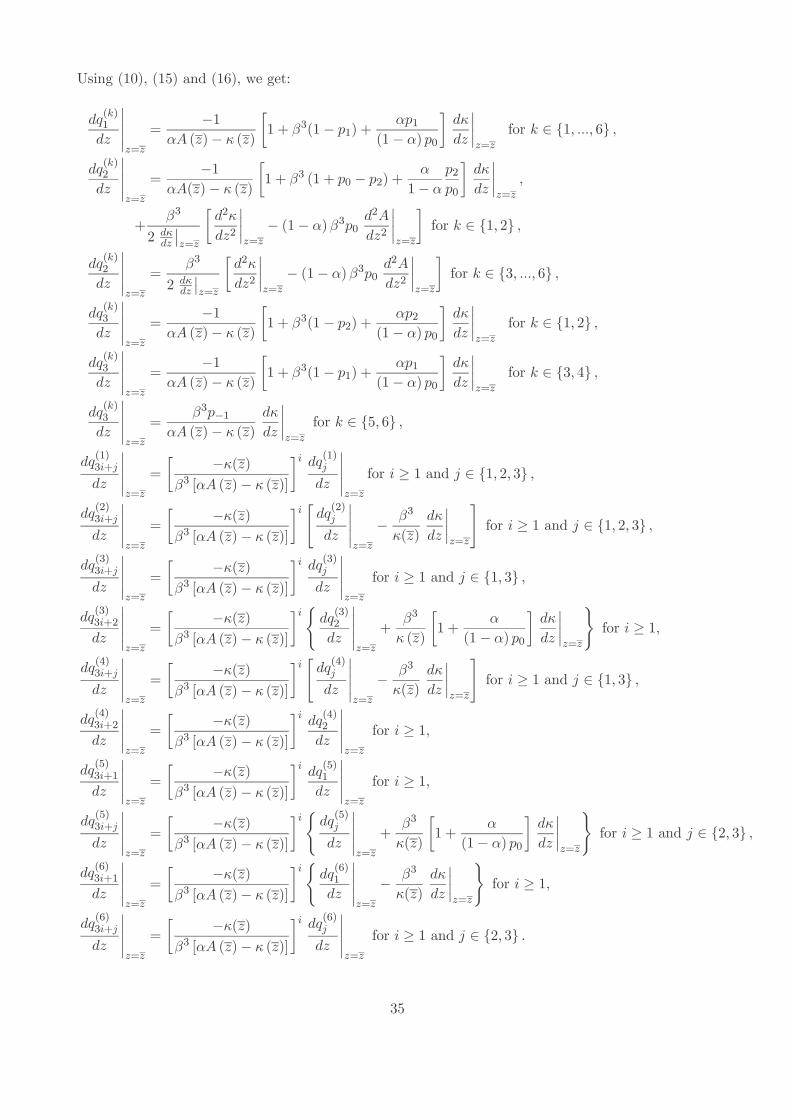
Using (10), (15) and (16), we get:

dq(k)1dz

∣∣∣∣∣z=z=

−1

αA (z)− κ (z)[1 + β3(1− p1) + αp1

(1− α) p0] dκdz∣∣∣∣z=z

for k ∈ 1, ..., 6 ,

dq(k)2dz

∣∣∣∣∣z=z=

−1

αA(z)− κ (z)[1 + β3 (1 + p0 − p2) + α

1− αp2p0] dκdz∣∣∣∣z=z

,

+β3

2 dκdz∣∣z=z

[ d2κdz2∣∣∣∣z=z

− (1− α)β3p0 d2Adz2

∣∣∣∣z=z

]for k ∈ 1, 2 ,

dq(k)2dz

∣∣∣∣∣z=z=

β32 dκ

dz∣∣z=z

[ d2κdz2∣∣∣∣z=z

− (1− α)β3p0 d2Adz2

∣∣∣∣z=z

]for k ∈ 3, ..., 6 ,

dq(k)3dz

∣∣∣∣∣z=z=

−1

αA (z)− κ (z)[1 + β3(1− p2) + αp2

(1− α) p0] dκdz∣∣∣∣z=z

for k ∈ 1, 2 ,

dq(k)3dz

∣∣∣∣∣z=z=

−1

αA (z)− κ (z)[1 + β3(1− p1) + αp1

(1− α) p0] dκdz∣∣∣∣z=z

for k ∈ 3, 4 ,

dq(k)3dz

∣∣∣∣∣z=z=

β3p−1αA (z)− κ (z)

dκdz∣∣∣∣z=z

for k ∈ 5, 6 ,

dq(1)3i+jdz

∣∣∣∣∣z=z=

[−κ(z)

β3 [αA (z)− κ (z)]]i dq(1)j

dz∣∣∣∣∣z=z

for i ≥ 1 and j ∈ 1, 2, 3 ,

dq(2)3i+jdz

∣∣∣∣∣z=z=

[−κ(z)

β3 [αA (z)− κ (z)]]i [ dq(2)j

dz∣∣∣∣∣z=z

−β3κ(z)

dκdz∣∣∣∣z=z

]for i ≥ 1 and j ∈ 1, 2, 3 ,

dq(3)3i+jdz

∣∣∣∣∣z=z=

[−κ(z)

β3 [αA (z)− κ (z)]]i dq(3)j

dz∣∣∣∣∣z=z

for i ≥ 1 and j ∈ 1, 3 ,

dq(3)3i+2dz

∣∣∣∣∣z=z=

[−κ(z)

β3 [αA (z)− κ (z)]]i dq(3)2

dz∣∣∣∣∣z=z

+β3κ (z)

[1 +

α(1− α) p0

] dκdz∣∣∣∣z=z

for i ≥ 1,

dq(4)3i+jdz

∣∣∣∣∣z=z=

[−κ(z)

β3 [αA (z)− κ (z)]]i [ dq(4)j

dz∣∣∣∣∣z=z

−β3κ(z)

dκdz∣∣∣∣z=z

]for i ≥ 1 and j ∈ 1, 3 ,

dq(4)3i+2dz

∣∣∣∣∣z=z=

[−κ(z)

β3 [αA (z)− κ (z)]]i dq(4)2

dz∣∣∣∣∣z=z

for i ≥ 1,

dq(5)3i+1dz

∣∣∣∣∣z=z=

[−κ(z)

β3 [αA (z)− κ (z)]]i dq(5)1

dz∣∣∣∣∣z=z

for i ≥ 1,

dq(5)3i+jdz

∣∣∣∣∣z=z=

[−κ(z)

β3 [αA (z)− κ (z)]]i dq(5)j

dz∣∣∣∣∣z=z

+β3κ(z)

[1 +

α(1− α) p0

] dκdz∣∣∣∣z=z

for i ≥ 1 and j ∈ 2, 3 ,

dq(6)3i+1dz

∣∣∣∣∣z=z=

[−κ(z)

β3 [αA (z)− κ (z)]]i dq(6)1

dz∣∣∣∣∣z=z

−β3κ(z)

dκdz∣∣∣∣z=z

for i ≥ 1,

dq(6)3i+jdz

∣∣∣∣∣z=z=

[−κ(z)

β3 [αA (z)− κ (z)]]i dq(6)j

dz∣∣∣∣∣z=z

for i ≥ 1 and j ∈ 2, 3 .

35

Using p1 = pAp2 + (1− pA) p0, we end up with:

dU I1

dz∣∣∣∣z=z

=dκdz∣∣z=z

κ (z) + β3 [αA (z)− κ (z)] κ (z)αA (z)

[1 + p0β4 + pAβ (1 + β) + (1− pA) pBβ2]

+κ (z)

(1− α) p0A (z)[(1 + β4 + β5) p1 + pAp2β (1 + β) (1− β3)+ (1− pA) pBp1β2 (1− β3)]

+β3α

(1− β) (1− α) p0[p1 (1− β + β3)+ pAp2β (1− β2)+ (1− pA) pBp1β2 (1− β)]

+β4κ (z) [αA (z)− κ (z)]

2αA (z)

(1− α)β3p0 d2A

dz2∣∣∣z=z −

d2κdz2∣∣∣z=z( dκ

dz∣∣z=z

)2

.

For the entrepreneurs:

V I1 (z) = pAβ3

p2∑+∞

i=0 βi[(1− α)A(z)− κ(z)

q(1)i+1 (z)

]

+(1− p2)[∑2

i=0 βi[(1− α)A(z)− κ(z)

q(2)i+1 (z)

]+∑+∞

i=3 βi[(1− α)A(z)− κ(z)

q(2)i+1 (z)

]]

+(1− pA)β3pB[p1[∑

i∈N1 βi[(1− α)A(z)− κ(z)

q(3)i+1 (z)

]+ β

[(1− α)A(z)− κ(z)

q(3)2 (z)

]]

+(1− p1)[∑

i∈0,2 βi[(1− α)A(z)− κ(z)

q(4)i+1 (z)

]+∑

i∈N0,2 βi[(1− α)A(z)− κ(z)

q(4)i+1 (z)

]]]

+(1− pB)[p−1

[∑

i∈N1,2 βi[(1− α)A(z)− κ(z)

q(5)i+1 (z)

]+∑2

i=1 βi[(1− α)A(z)− κ(z)

q(5)i+1 (z)

]]

+(1− p−1)[(1− α)A(z)− κ(z)

q(6)1 (z) +∑+∞

i=1 βi[(1− α)A(z)− κ(z)

q(6)i+1 (z)

]]].

Using (10) and p1 = pAp2 + (1− pA) p0, we end up with:

dV I1

dz∣∣∣∣z=z

=dκdz∣∣∣∣z=z

−1

1− β[(1− β) + p1β3 + (1− pA) pBβ2 (1− β) + pAβ (1− β2)]

+1

p0 (1− β)[p1 (1− β + β3)+ pAp2β (1− β2)+ (1− pA) pBp1β2 (1− β)]

−κ (z)

A (z)αβ3[1 + p0β4 + pAβ (1 + β) + (1− pA) pBβ2]

−κ (z)

A (z) (1− α) p0β3[(1 + β4 + β5) p1 + pAp2β (1 + β) (1− β3)+ (1− pA) pBp1β2 (1− β3)]

−βκ (z) [αA (z)− κ (z)]

2αA (z)

(1− α)β3p0 d2A

dz2∣∣∣z=z −

d2κdz2∣∣∣z=z( dκ

dz∣∣z=z

)2

.

36

H Conditions imposed on the parameters

In the general case (subsections 4.1 and 4.3), the relevant parameters are α, β, κ (z), κ (z), A (z),A (z), p0, λ, N and τ t for t ∈ 1, ..., N. The conditions imposed on them are 0 < α < 1, 0 < β < 1,κ (z) > κ (z) > 0, A (z) > A (z) > 0, 0 < p0 < 1, 0 < λ < 1, N ∈ N∗, τ t > 0 for t ∈ 1, ..., N,(1), (2), (3), (5), (6), (8), (9), (17), (18), (19), (20), as well as the necessary and sufficient condition

to get: ∀t > N , zt = z if the new technology turns out to be good, and zt = z otherwise, whatever(zt, ct, qt) ∈ Ft ×R+ ×R+∗ for t ∈ 1, ..., N.

In the simple case (subsection 4.2), the relevant parameters are α, β, κ (z), dκdz∣∣z=z, A (z), dA

dz∣∣z=z,

p0, λ, N and dτ tdz∣∣z=z for t ∈ 1, ..., N. The conditions imposed on them are those corresponding

to the conditions imposed in the general case (listed above), to which should be added the following

conditions: N = 3, dτ1dz∣∣∣z=z =

dτ3dz∣∣∣z=z = 0, (10), (11) and (14). Together, these conditions are

equivalent to the following ones7: 0 < α < 1, 0 < β < 1, κ (z) > 0, dκdz∣∣z=z > 0, A (z) > 0, dA

dz∣∣z=z > 0,

0 < p0 < 1, 0 < λ < 1, N = 3, dτ1dz∣∣∣z=z =

dτ3dz∣∣∣z=z = 0, (1), (2), (3), (10), (11) and (14). It is easy to

see that the set of parameters satisfying all these conditions is not empty. As a consequence, neither

is the set of parameters satisfying all the conditions imposed in the general case.

7 In particular, the conditions p0 < 1 and (10) imply that the last condition in the general case is satisfied in thesimple case. Indeed, on the one hand, ∀ (zt, ct, qt) ∈ Ft × R

+ × R+∗ for t ∈ 1, ..., N, we have: ∀t > N , qt is close toβ3. On the other hand, given (10) and p0 < 1, we have β3 > B (z) > 0. These two results together imply that ∀t > N ,qt > B (z) > 0 and therefore (following a reasoning similar to that of the beginning of appendix F) ∀t > N , It = 1 if thenew technology is good and It = 0 otherwise.

37