Embed Size (px)
Citation preview

Payer Type and the Returns to Bypass Surgery:Evidence from Hospital Entry Behavior
Michael Chernew, Ph.D.1Department of Health Management and Policy
Department of EconomicsDepartment of Internal Medicine
The University of Michigan,and NBER
Gautam Gowrisankaran, Ph.D.Department of EconomicsUniversity of Minnesota,
Federal Reserve Bank of San Francisco,and NBER
A. Mark Fendrick, M.D.Department of Internal Medicine
Consortium for Health Outcomes Innovation and Cost Effectiveness StudiesThe University of Michigan
December 11, 2001
Acknowledgments: We thank Rajesh Bandekar for able research assistance and the Data User SupportGroup of the State of California Office of Statewide Health Planning and Development for provision ofthe data. We acknowledge helpful comments received from Dan Ackerberg, Lanier Benkard, SteveBerry, Jim Burgess, David Cutler, Randy Ellis, Joseph Newhouse, Ariel Pakes, John Rust, seminarparticipants from several institutions and two anonymous referees. The views expressed herein are solelythose of the authors, and do not represent those of the Federal Reserve Bank of San Francisco or of theFederal Reserve System.
1 Michael E. Chernew, Ph.D. University of Michigan, School of Public Health, 109 Observatory, Ann Arbor, MI48109-2029; Phone: (734)936-1193, Fax: (734)764-4338, [email protected].

Payer Type and the Returns to Bypass Surgery:Evidence from Hospital Entry Behavior
Abstract
In this paper we estimate the returns associated with the provision of coronary artery bypass graft(CABG) surgery, by payer type (Medicare, HMO, etc.). Because reliable measures of prices andtreatment costs are often unobserved, we seek to infer returns from hospital entry behavior. We estimatea model of patient flows for CABG patients that provides inputs for an entry model. We find that FFSprovides a high return throughout the study period. Medicare, which had been generous in the early1980s, now provides a return that is close to zero. Medicaid appears to reimburse less than averagevariable costs. HMOs essentially pay at average variable costs, though the return varies inversely withcompetition.

1
1. Introduction
In this paper, we seek to estimate the returns associated with the provision of coronary artery
bypass graft (CABG) surgery by payer type. CABG surgery is used to treat coronary artery disease,
which is a leading cause of death, morbidity and expense in the United States. CABG is an expensive,
technologically intensive procedure provided to over 350 thousand Americans annually, with utilization
growing at over 9% a year.2 Returns, which capture all the benefits to the hospital associated with the
per-case provision of CABG, will reflect financial and other rewards for use of this procedure.
Variations in returns raise both efficiency and equity concerns. Overly generous payments by
prominent insurers such as Medicare may induce excessive entry by hospitals into the market for CABG
as well as over-usage among hospitals that provide CABG. The possibility of excessive provision of
CABG is of particular importance since the rapid rise in health care expenditures in recent years has been
attributed to the growing diffusion and utilization of expensive high technology services such as CABG
[Cutler and McClellan (1996)].
Variations in payment rates among insurers, which would generate variations in returns, have led
to charges that some payers are not paying their ‘fair share’. Considerable attention has been devoted to
measuring ‘cost shifting’, the practice of raising the prices to some payers to cover insufficient payments
from other payers [Hadley and Feder (1985), Morrisey (1995)]. If the Medicare payment rates are too
high, taxpayers are subsidizing health care providers, or perhaps subsidizing individuals covered by
insurers who pay less for care. Large, self-insured employers, who often pay more for services than
managed care plans, complain that they are subsidizing other employers with different insurance types.
To the extent that cost savings associated with HMOs reflect price advantages made possible by generous
payments from other payers, HMO induced savings may be short lived.
The direct way to uncover margins, a prime component of returns, is to find or estimate prices
and costs. While Medicare payment rates for CABG are publicly available,3 prices paid by other insurers,
particularly HMOs, are difficult to observe. It is generally thought that commercial and Blue Cross
insurers pay the most for services, followed by Medicare, managed care plans, and Medicaid.
2 National Center for Health Statistics (1997) and National Center for Health Statistics (1986).3 In 1991, average Medicare reimbursement for CABG was $32,117 [Cutler and McClellan (1996)].
2
Even though we have a general sense of relative payment generosity, observation of costs would
be required to determine whether some payers, such as managed care plans, are paying below costs or
merely covering the expenses of their enrollees. Relative margins may not map directly to payment rates
because of variation in costs. Measurement of costs by payer and service type is inherently difficult
because hospital accounting systems and case-mix differences make it difficult to directly attribute costs
to specific patients or services. Costs for different types of patients are likely to be very different.
While it is difficult, if not impossible, to estimate returns directly, there is an alternative method
to infer returns, which is to observe entry into the market for CABG surgery. We make the assumption
that hospitals that do not already provide CABG will choose to enter into the CABG market only if they
receive sufficient returns. Returns are then linked to entry behavior: the higher the variable returns are,
the more likely a hospital will be to enter into the CABG market. Over the period of our study the
number of CABGs rose about 5% per year and the number of hospitals offering CABG rose from 84 to
126. About one third of potential entrants for CABG entered over the sample period. This provides us
with a reasonably sized data set on entry behavior.
Our use of entry as a tool to uncover underlying industry parameters has support in the empirical
industrial organization literature [Bresnahan and Reiss (1991), Berry (1992)]. In contrast to these earlier
works, we construct a model where we endogenously determine and test for the appropriate market
definition. We are able to do this by combining detailed patient discharge data with the hospital entry
data. Additionally, as we discuss below, our results appear to be confirmed by economic theories and
independent accounting data, which validates the use of entry as a tool to uncover fundamental firm
parameters. Thus, one can think of using entry to examine many aspects of hospital behavior where
prices or costs are not estimable, such as economies of scope between different services and the nature of
competition between insurance providers and hospitals.
The focus of this research is on analyzing the variable returns to CABG surgery. Our entry model
is based on a hospital ‘return’ function that assumes that average returns for CABG are different for each
of six payer types (Medicare, Medicaid, HMO, FFS, Other Public Coverage and Other Private
Coverage).4 We express total variable returns as the sum of the returns received from patients of each
4 The return function serves as a profit function, but conceptually allows non-financial benefits to be associated withprovision of CABG and is perhaps more semantically appropriate given the prevalence of not-for-profit hospitals inour sample.
3
payer type. These returns are in turn given by the volume of patients by payer type, times the average
return for that payer type. As we do not observe volumes for hospitals that do not enter, we need to
predict volumes. From our return function, if a payer is paying a positive average return, this will
generate a positive correlation between volume for that payer type and the probability of entry, and vice
versa. Thus, assuming that we can approximate predicted volumes, we can infer relative average returns
by regressing the volumes by payer type on the entry decision, using a duration model approach.
We predict volumes for potential entrants using conditional logit models of patient flows for
CABG services. We allow hospital choice for CABG to be influenced by the insurance type of the
patient, distance from the patient to the hospital, and various hospital attributes such as ownership,
number of beds, and lagged cardiac and non-cardiac volume. Using our estimated logit coefficients, we
then predict volumes for potential entrants by simulating the addition of the entrant into the market and
calculating expected patient flows to that hospital. Econometric tests confirm that we are able to closely
estimate volume, even for entrants.
The identification of returns in our model is based on the differences in expected patient flows by
payer type across hospitals (HMOs, FFS, etc.). For example, if entry is likely for hospitals that would
receive many FFS patients conditional on entry, we will tend to infer that FFS coverage is associated
with positive returns. The differences in expected patient flows by payer types are in turn identified by
the level of competition for CABG patients from nearby hospitals, the number of patients by payer type
in the geographic area surrounding a hospital, and the probability of admission by payer type for non-
cardiac services and cardiac services in previous years.
Identification from the geographic distribution of patients is common in this literature (Cutler
and McClellan, 1996; Baker and Wheeler, 1998; Spetz and Baker, 1999). Our model builds on this
identification by adding in the effect of competition and specialization by payer type. Thus, we will view
two hospitals in areas that have the same number of FFS patients differently if there are different
numbers of existing or potential CABG providers in those areas, or if those hospitals admit different
numbers of FFS patients for non-cardiac services.
Our results confirm the general opinion that average returns from FFS insurers are the greatest,5
5 We use the term FFS to refer to Commercial and Blue Cross/Blue Shield plans. This category includes a variety ofpartly managed care plans such as Point of Service plans, which may not reimburse on a fee-for-service basis.

4
followed by Medicare, HMOs, and Medicaid. Consistent with published ProPAC figures,6 our estimates
suggest that at the start of our study period Medicare provided a large return that had disappeared by the
end of the study period. Economic theory suggests that those payers willing to shop for care would
receive prices approximating costs and our results confirm this intuition, as HMOs appear to be
providing hospitals with returns close to zero. Finally, unlike returns for other payers, returns from
HMOs vary inversely with the degree of market competitiveness, consistent with competitive bidding for
hospital services by HMOs.
We explore several econometric issues, including the specification of the duration model, the
ability of entry to expand the market size, the possibility of unobserved market traits that are correlated
with both entry and payer mix, and the potential endogeneity of predicted volume. Estimates accounting
for these factors support the conclusions reached in our primary analysis.
The remainder of this paper is divided as follows. In Section 2, we detail the model. Section 3
outlines our data and construction of entry variables. Section 4 provides our results. Section 5 concludes.
2. Model
In order to estimate CABG returns, we specify two different models, a patient flow model and a
hospital entry model. For the entry model, we take as our sample the set of potential entrants into the
market for CABG services and regress the decision of whether to enter on anticipated volume by payer
type, controlling for hospital-specific attributes. We define potential entrants to be the set of hospitals
that were admitting patients in the current year, that did not perform CABGs in the previous year, and
that provided some cardiac service (cardiac catheterization, angioplasty or CABG) at some point in the
period of our study.7 We estimate the entry model using nine years of data. Our primary interest is to
estimate the coefficients of the entry model. With the assumptions of optimizing behavior and rational
expectations, these coefficients are interpretable as average variable returns.
6 Prospective Payment Assessment Commission (1995).7 Virtually all potential entrants provided cardiac catheterization, a less technologically advanced cardiac service,prior to entering the market for CABG. Thus our set of potential entrants is largely the set of hospitals providingcatheterization but not CABG. We also experimented by adding all hospitals with 200 or more beds to the list ofpotential entrants. This did not substantively change any results.

5
In order to estimate the coefficients of the entry model, we need measures of expected volume by
payer type for the set of potential entrants. This is where we use the patient flow model. We estimate
choice of hospital using a reduced-form conditional logit framework where choice is assumed to be a
function of the patient’s insurance type, distance to each hospital and various hospital characteristics. To
calculate volume for potential entrants, we then make use of the fact that potential entrants are all
existing hospitals, and hence have well-defined values for the variables that we assume affect hospital
choice, and thus patient flows. Using our estimated discrete choice model, we simulate the addition of a
potential entrant into the industry, and calculate its predicted volume by payer type conditional on it
entering. By doing this for every potential entrant separately, we then obtain the expected volume for
each potential entrant were it to decide to enter. These we then use as explanatory variables for our entry
model.
We now proceed to detail the entry model and patient flow model.
2.1 A model of entry
We posit an optimizing model of entry. For the purposes of this study, we will assume static
optimization, so that returns in the year subsequent to entry do not affect the entry decision. This is
equivalent to the assumption that hospitals have a discount factor of 0. While this assumption is also
likely to be false, hospitals have the option to enter in the subsequent period. If the decision to enter does
not cause the state space to change, then firms should only examine the increment to returns from current
period CABG volume in their entry decision. The only caveat to this is that the decision to not enter may
precipitate a rival to enter, which would then change the state space by lowering the future returns from
entry.
We write total returns for a potential entrant j in year t as :
(1) ( )m
j,t h , j,t h, j,t 1, j,t m, j,t j,th 1
TR P Q C Q , ,Q K=
= − +� � .
where h indexes m payer types, which are Medicare, Medicaid, HMO, FFS, other public and other
private; t,j,hP denotes average per CABG reward (largely price) from payer h to hospital j in year t; t,j,hQ

6
denotes average quantity from patients with insurance from payer h to hospital j in year t; ( )C denotes
variable costs; and j,tK denotes the sum of fixed and sunk benefits of entry for hospital j in year t.
We assume that variable costs are separable by payer type. Thus ( )1, j,t m, j,tC Q , ,Q� becomes
( )� t,j,ht,j,h QAVC , where AVC denotes average variable costs. With this assumption, the returns
equation reduces to:
(2) ( )m m
j,t h, j,t h, j,t h, j,t j,t h, j,t h, j,t j,th 1 h 1
TR Q P AVC K Q R K= =
= − + ≡ +� � ,
where t,j,hR is defined to be the average return by payer type and hospital.
We assume that hospitals will enter if total variable returns exceed the threshold t,jK . Profit-
maximization is consistent with t,jK equal to the negative of the fixed and sunk costs of entry. However,
many hospitals are not-for-profit and these hospitals may have different thresholds for entry. Thus, we
allow t,jK to be a function of hospital characteristics that might influence the objective function
including ownership status (e.g. not-for-profit) and medical school affiliation.
Specifically, we define:
(3) j,t j,t j,tK Z e= γ + ,
where j,tZ includes hospital-specific variables that might influence the objective function as well as year
dummies, and t,je represents the unobservable component of t,jK . The year dummies will capture trends
in entry costs as well as changes in the fixed and sunk benefit of entry for the average potential entrant
caused by changes in the pool of potential entrants over time.
We make one major simplifying assumption in our base model that we later relax: that the degree
of market power is similar enough within a payer type so that the average returns are the same within
payer type across different hospitals and different years. For Medicare (where prices are fixed), this
implies that hospital costs for Medicare patients do not vary by hospital; for other payer types the
assumption is similar. Given our assumptions, hospital j will enter at the first year t when:

7
(4)m
h, j,t h j,t j,th 1
Q R Z e 0=
+ γ+ >� .
From (4), one can see that in order to estimate average returns, it is necessary to be able to predict the
quantities that potential entrants face should they choose to enter. We do not use a model of hospital
pricing behavior to estimate t,j,hQ . Instead, our approach is to estimate t,j,hQ using a reduced-form
patient flow model that we detail in Section 2.2.
The variance of t,je is not identified from the data. Hence, for our base results, we normalize
)1,0(N~e t,j , iid. In this case, the estimated returns coefficients should be interpreted as their true values
divided by a common constant, the standard deviation of t,je . With this distributional assumption, we can
write the conditional probability of entry for a potential entrant as a standard probit:
(5) ( )m
j,t h , j,t h j,th 1
Pr Entry j not in at t 1 Q R Z=
� �− = Φ + γ� �� �� ,
where ‘Φ’ indicates the standard normal cdf. We estimate this specification by using maximum
likelihood on the set of potential entrants. Since potential entrants are dropped from the sample once they
enter, (5) is a duration model with a time varying hazard, where the ‘hazard’ is entry into CABG.
To verify the robustness of our results, we also examine a couple of alternate specifications
similar to (5). First, we estimate a version where we relax the iid assumption on t,je . Specifically, we
allow the error terms for a given hospital across time to follow an AR(1) process, which implies that
(6) t sj,t j,t sCorr e ,e −
−� � = ρ� � ,
where ρ is an additional parameter to estimate. This model will capture unobserved hospital-specific
effects. Because we have nine time periods, a direct maximum likelihood estimation of the serially
correlated probit model would involve nine-dimensional normal integration for each hospital, which is
not computationally feasible. Instead, we use the method of simulated likelihood combined with the
GHK algorithm [Geweke (1989), Hajivassiliou, McFadden and Ruud (1996), and Keane (1994)] to
efficiently simulate the normal densities.

8
Second, we estimate a Cox proportional hazard model. In this model, the hazard of entry for
hospital j at time t̂ that lies between t–1 and t is given by:
(7) ( ) ( )m
ˆ 0 h, j,t h j,tj,th 1
ˆ ˆf Entry j not in at t h t exp Q R Z=
� �= + γ� �� �� ,
where ( )0ˆh t is a non-parametric function of time. The hazards stemming from (5) – (7) are similar,
particularly since the probit specifications contain time dummies. D’Agostino et al. (1990) and Allison
(1995), demonstrate the close correspondence between these two types of duration modeling
specifications. We estimate (7) because it provides a different functional form, and one that is more
standard, for the hazard. However, unlike the probit specifications, we are not aware of any functional
form for the t,je ’s in (4) that would generate (7). The Cox model can be estimated via conditional
maximum likelihood.
We limit our sample to those hospitals that had not entered by the start of our study period, 1986.
This excludes 85 hospitals, or two-thirds of hospitals that ultimately entered. We do not address this left
censoring for both conceptual and practical reasons. Conceptually, the motivation for early entrants may
differ from that of late entrants. Hospitals strongly inclined to adopt new technology regardless of returns
are likely to be early adopters. Therefore, we think that the coefficients may not be stable between early
and late entrants. On a practical level, our model posits entry as a function of time-varying regressors,
including estimated volumes. Although we can observe the year of entry for all hospitals from AHA data
(even those that entered before our study period), we do not have the data necessary to estimate predicted
volume prior to our study period.
We estimate (5) – (7) using predicted values for t,j,hQ for all potential entrants, where these
predicted volumes are derived from our patient flow model, as described in Section 2.2. We use predicted
volume instead of actual volume conditional on entry because we do not observe the volume that non-
entrants would have received had they entered. Moreover, actual volume in the year of entry is a poor
measure of the steady state volume, since hospitals often enter in the middle of a year.
Our predicted values for t,j,hQ are a proxy for the true expected annual value of t,j,hQ . The
difference between the predicted and true volumes is either proxy error or measurement error, depending
on whether the difference is correlated with the true or predicted volume, respectively. Measurement

9
error would occur if our true volumes were imprecisely estimated due to a limited sample size. Because
our predicted volumes are based on our patient flow model with over 20,000 patients in each year, we
feel that measurement error will be negligible. Thus, any difference is likely attributable mostly to
unobserved hospital traits that affect true expected volume but are uncorrelated with our predicted
volume, i.e. proxy error. Unlike measurement error, proxy error will not bias the coefficients but will
simply be added to the entry model error.
There are also potential concerns that the predicted volumes may be biased in a variety of ways.
For instance, there is the possibility that actual entrants may have some unobserved advantage that leads
them to receive a higher volume than potential entrants who do not enter. Additionally, the predicted
volumes may be endogenous because of competitive interactions. In Section 4, we try to assess the
magnitude of these issues and correct for them.
Lastly, we note that we have made a number of simplifying assumptions for our base case model
in (5), which we later relax. First, we assume that average returns for a given payer type do not vary
across time and hospital. Because the level of competition may differ for different hospitals, returns may
vary by hospital for some payer types. Additionally, exogenous changes in institutional structures (e.g.
Medicare payment rate changes) may result in a variation in average returns across time. To mitigate this
problem we examine specifications where returns are allowed to be a function of time or of the level of
hospital competition.
2.2 Predicting volume
Our estimates of predicted volume t,j,hQ are based on a utility maximizing model of hospital
selection. The underlying econometric model is based on the assumption that the utility associated with
any particular hospital for CABG reflects hospital characteristics, the distance from the patient’s
residence to the hospital, and the patient’s insurance type. The utility function is a composite of patient,
physician, and insurer utility, all of which influence hospital choice. The setup is analogous to the
conditional choice model of McFadden (1973), (1974). We specify the utility derived if individual ‘i’
chooses hospital ‘j’ as:
(8) ( ) ijT,IijT,Ij,Iij iiiiiDfXU ε+λ⋅+β=

10
where iI is patient i’s insurance type (which is one of six listed above), iT is the year in which the
patient receives treatment (ranging from 1986 to 1994), j,IiX is a vector of hospital characteristics that
can vary by payer type (which is detailed in Section 3), ijD is the distance in kilometers from patient i’s
residence to hospital j, ( )λβ, are vectors of parameters, and ε ij is a Type I extreme value stochastic term
capturing preferences for unobserved hospital attributes.
Explanatory variables are intended to capture hospital attributes that might attract patients, their
physicians, or even their insurers. Perhaps most important of these variables is the distance between thepatient’s residence and the hospital, ijD . This distance is measured as the straight-line distance between
the zip code centroid of the patient’s residence and the hospital. Other studies have found distance to be a
primary determinant of patient flows [Luft et al. (1990), Chernew et al. (1998), Burns and Wholey
(1992)]. Our model includes two measures of distance; specifically, we let
( ) ( ) ( )( )2
ij ij ijf D log 1 D , log 1 D� �= + +� � .
If individual i receives treatment at hospital j, it is assumed that the utility associated with
hospital j must exceed that of all other hospitals that person i could have chosen. In our primary analysis,
we do not allow for an outside alternative for the practical reason that we only observe the set of patients
who are treated for CABG. In our sensitivity analysis, we adjust for the percentage of heart disease
patients receiving CABG.
We define Yij = 1 when individual i is treated at hospital j and Yij = 0 otherwise. Then, we
obtain the usual logit formula:
(9) { } ( )( )( )( )�
∈
λ+β
λ+β==
i
iiiii
iiiii
CkT,IikT,Ik,I
T,IijT,Ij,Iij DfXexp
DfXexp1YPr ,
where Ci is the choice set for patient i.
The choice set Ci for individual i is comprised of all hospitals offering CABG within a 120-
kilometer market area of her residence. This distance threshold captures over 90% of all patients. Many
of the remaining patients likely have miscoded distances or received care as part of an emergency
episode when they were away from home.

11
We estimate (9) using maximum likelihood. Given the logit error term, we can estimate (9)
separately by payer type and year. Estimated coefficients from (9) can be used to predict volume by payer
for potential entrants. We assume rational expectations: potential entrants know which other hospitals
will be in the market and the aggregate volume of CABG. Predicted volume for hospital j, if it enters, is
computed as:
(10)( )( )
( )( )h , j
i
h, j h ij hh, j
i M h,k h ik hk C j
ˆ ˆexp X f DQ̂ ˆ ˆexp X f D∈
∈ ∪
β + λ=
β + λ�
�
where j,hM is the set of all patients residing within a 120 kilometers market area of hospital j who are of
insurance type h.
There are a couple of features about our modeling of hospital choice that are of potential
concern. First, the logit distribution of the ε’s in (8) implies independence of irrelevant alternatives (IIA).
IIA implies that the probability of choosing a given hospital relative to another hospital is independent of
the other hospitals in the patient’s choice set. If some hospitals are closer substitutes to a given hospital
than others, IIA will be violated. Although IIA will apply at the individual level, this fear is somewhat
mitigated by the fact that we use patient specific data (namely geographical location and insurance type).
Because of this, IIA will not hold at the aggregate level. Recall from (5) that we are only interested in
aggregate volume by payer type for each hospital. Moreover, Phibbs et al. (1993) estimated similar
models of patient flows for birthing services and could not reject the hypothesis of IIA.
Another issue is the possibility of unobserved hospital specific attributes uncorrelated with the
X’s. Such hospital-specific factors will generate correlations among the ε’s. This will result in
overestimated precision on the coefficients from the patient flow model. Alternative methods, using
grouped data, could be used to address this problem [Berry (1994)], but studies of patient flows suggest
that estimation using individual level data is more stable [Garnick et al. (1989)]. Moreover, our
inferences from the entry model do not require use of the variance of the coefficients of the patient flow
model. Therefore, underestimated standard errors from the patient flow model do not affect our
conclusions. To check the stability of our estimates, we examine the correlations between predicted
volumes generated from coefficients estimated on data from different years. For example, we measure

12
the correlation between predicted 1994 volume using coefficients based on 1994 data with predicted
1994 volume using coefficients based on 1992 data.
Lastly, we note that we did not include measures of prices in our choice equation. This decision
was made for two reasons. First, prices are not observed for most payer types and hence cannot easily be
used.8 Second, we view the hospital choice equation as a reduced-form equation that encapsulates
optimizing pricing behavior. As an endogenous variable chosen by hospitals, price should not be
included in the set of explanatory variables.
Despite these concerns about the entry model, our inference regarding returns requires primarily
that we approximate predicted patient volumes well. A more detailed model might explain patient flows
better, but as the results presented below indicate, our existing model does a reasonable job and is
sufficient for our purposes.
3. Data
Our data come primarily from hospital discharge records for the state of California supplied by
the Office of Statewide Health Planning and Development. The data contain information on every
discharge from hospitals in California between 1984 and 1994 (about 300,000). For each discharge, we
observe a hospital ID, principal source of payment (payer type), 5 procedure codes, and the zip code of
the patient’s residence. We merged this with hospital-specific data from the American Hospital
Association to capture the zip code of the hospital and hospital characteristics. We used the Census
TIGER database and standard formulas to compute straight-line distances between hospitals and the zip
code centroid of patient residences.
Patients were identified as CABG, PTCA or cardiac catheterization patients if any of the
International Classification of Diseases Ninth Revision (ICD-9) procedure codes indicated one of these
procedures.9 We were broad in our definition of procedure codes because we want to capture all of the
8 Medicare prices are observed. Because Medicare does not steer patients to hospitals, these prices are unlikely toaffect patient flows. Moreover, there is little variance in Medicare price.9 For CABG, we use ICD-9 procedure codes of 35.1x - 35.7x, 35.90 - 35.95, 35.98, 35.99, 36.03, 36.1x, 36.2x,36.9x, 37.1x, 37.24, and 37.3x. For PTCA, we use codes of 35.96, 36.01, 36.02, 36.05 and 36.06. For cardiaccatheterizations, we use codes of 36.04, 37.21 - 37.23, 37.25, 88.50, 88.52 - 88.57.
13
possible returns from procedures potentially performed using the CABG facilities. Some of the included
procedures could be performed even without the specialized facilities that we are studying.
We discarded patients residing outside of California or with missing distance data. We also
omitted patients who traveled further than 120 kilometers for care. Lastly, we omitted patients who were
treated at hospitals that were not ‘in’ the CABG market. Collectively these sample restrictions reduced
our sample by 10 percent.
In order to estimate our model of entry, we need to measure which hospitals were active in the
market in any year. We infer participation in the CABG market by aggregating the discharge data to the
hospital level, and observing the number of patients receiving CABG at each hospital.
We considered hospitals to be ‘in’ the market for CABG in any particular year if they performed
more than 20 CABGs in that year. We used the 20-procedure threshold because our broad definition of
CABG and miscoding may erroneously indicate entry and very low volumes may be performed at
facilities not genuinely ‘in’ the market for providing CABG. This threshold minimized the problem of
erratic entry behavior; hospital entering, exiting, and re-entering the market over our study period.10
The final data issue we addressed was treatment of hospitals owned by the Kaiser Foundation
Health Plan. Kaiser is by far the dominant HMO in California and owns and operates its own hospitals.
These facilities largely treat Kaiser enrollees. For some tertiary services, including CABG, Kaiser
supplements its capacity by contracting with other hospitals to provide the services to its enrollees. We
cannot identify Kaiser enrollees, but we can identify Kaiser owned facilities, most of which do not offer
CABG. Entry by Kaiser Foundation hospitals may reflect different factors than entry by other hospital
because entry decisions are made centrally and because Kaiser is primarily concerned with its enrollees.
When Kaiser hospitals are excluded from the base model, estimated returns from HMO payers switch
sign (from negative to positive), but remain statistically insignificant. Our other conclusions are robust to
exclusion of these Kaiser hospitals from the entry model. Because of space limitations, we do not present
the results that exclude Kaiser hospitals any further.11
10 Despite use of the 20-procedure threshold, there were 3 hospitals that displayed erratic entry behavior. Two ofthese three hospitals performed fewer than 20 procedures for a year or two after having higher volume earlier andthen returned to high volume. We considered those hospitals to be ‘in’ the market from the first year at which theyperformed 20 or more procedures. The third hospital was a Kaiser facility whose annual CABG volume fluctuatedbetween 3 and 20. We considered it not to be ‘in’ the CABG market during our study period.11 The issue of Kaiser hospitals is a subset of the larger issue of system affiliation. For other hospitals we do notobserve system affiliation. A complete model would adjust for cannibalization of volume between system partners.

14
Explanatory variables in our patient flow model (X’s) include several variables measuring
ownership status, teaching status, and hospital size. These traits may be related to perceptions of quality.
Our ownership categories include: public, for-profit, and private not-for-profit (omitted). We include two
measures of teaching status, hospital membership in the Council of Teaching Hospitals and the ratio of
residents and interns to beds. Hospital size is measured by the number of hospital beds.
The influence of hospital traits on patient flows may depend on insurance type, reflecting either
insurer influence over patient flows or systematic enrollment into certain types of coverage. For this
reason we interact all of the preceding explanatory variables with each year of data and with each of the
6 payer types: Medicare, Medicaid, HMO, FFS, other public and other private payers. The FFS group
corresponds to Commercial and BCBS insurers.12 Due to unreliability of coding for patients over the age
of 65 and differences between Medicare and non-Medicare HMOs, all patients over the age of 65 were
coded as Medicare patients even though some were enrolled in HMOs.13 In 1994, approximately 20% of
Medicare patients were enrolled in ‘at risk’ HMOs in California, though we cannot reliably identify
them.14 This figure was substantially smaller during most of our study period. The other private payer
type includes self-pay and indigent patients, which is where uninsured patients would be classified.
The X’s also include non-cardiac volume and lagged volume of cardiac services. We separately
measure 1- and 2-year lags for three types of cardiac services: cardiac catheterizations, percutaneous
transluminal coronary angioplasty (PTCA), and CABG. The lagged volumes are measured by payer type.
For non-cardiac and 1-year lagged CABG volume, we included the volumes for all payer types. For the Because the results seem insensitive to how the largest system is treated, we are less concerned about whether theresults would be sensitive to more fully modeling other systems.12 At a few hospitals in specific years, patients were missing payer type. This represented a very small percentage ofour sample (about 100 observations out of 300,000). For these patients, we imputed a payer type of Medicare if thepatient was aged 65 or more, and a payer type of HMO otherwise, because HMO was the most common at thesehospitals.13 The Office of Statewide Health Planning and Development (OSHPD) permits only one designated principalsource of payment. Hospitals were instructed to code the principal source of payment for Medicare recipientsenrolled in HMOs as ‘Medicare’ as opposed to ‘HMO’. Because not all hospitals complied, there is non-randomcoding of the over 65 population which may introduce systematic bias. Moreover, Medicare HMOs differ from otherHMOs for several reasons. First, during our study period a substantial number of Medicare HMO enrollees were in‘cost’ HMOs. These HMOs are not at risk for enrollee expenditures. Expenditures are passed through to Medicare.Second, Medicare HMOs were very new during this period and their contracting may have differed from other plans.Finally, Medicare beneficiaries can disenroll from their HMO monthly, unlike other HMO enrollees. This changesthe nature of the plan and may affect contracting between plans and providers. Thus elderly HMO beneficiaries maybe enrolled in fundamentally different types of plans. Because we coded all elderly as Medicare beneficiaries, ourcoefficients should be interpreted as reflecting the blend of HMO enrollment in Medicare.14 Prospective Payment Assessment Commission (1995).

15
other volume variables, we included the volume only for the own payer type. Additionally, we include
the patient’s race interacted with the percent of non-cardiac patients of that race discharged by the
hospital. The purpose of these variables is to capture unobserved traits, such as strength of referral
network, related to the demand for the hospital’s cardiac services. They allow us to more accurately
predict quantities within the context of the reduced-form choice model. We are not as interested in
testing hypotheses related to the preceding variables. For this reason the multicolinearity of many of the
explanatory variables is not of concern.
Because potential entrants will have no lagged CABG volume, the lagged variables capture any
negative association with new entrants. However, almost all entrants will have prior experience with
cardiac catheterization so the lagged cardiac catheterization volumes will capture the general presence of
the hospital in the market for cardiac services. Because we use lagged volumes, our entry equations only
include hospitals between 1986 and 1994, even though our data set extends from 1984 to 1994.
Explanatory variables in our entry model are much fewer. The main variables of interest are the
predicted volumes by payer type. The entry threshold variables (Z’s) include: beds, an indicator of for-
profit status, COTH membership, residents per bed and year dummies.
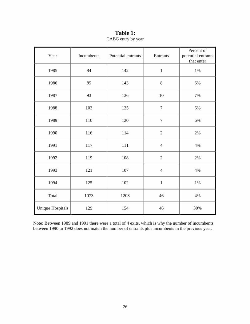
There were 46 hospitals that entered the market for CABG between 1985 and 1994. This
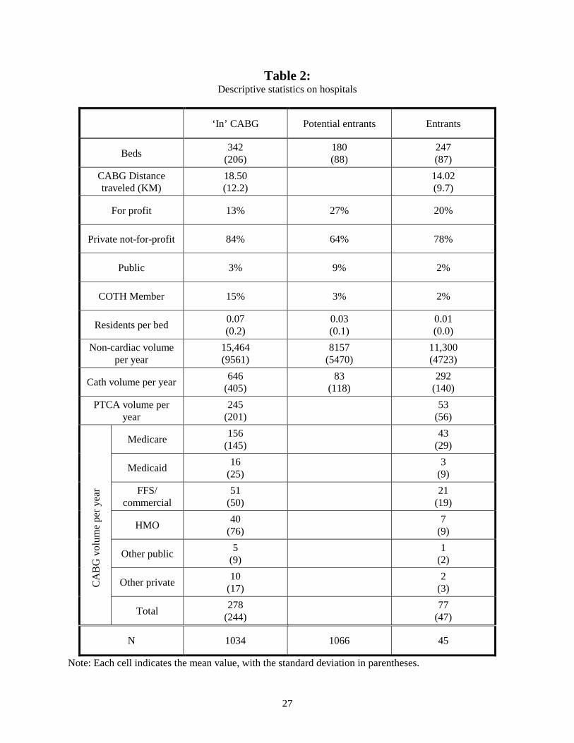
represents a growth of 49% over the 84 providers in 1984. Table 1 contains details on the pattern of entry
and number of incumbents. On average there were 121 potential entrants in each year, ranging from 142
in 1985 to 102 in 1994. Descriptive statistics for incumbents, potential entrants, and entrants are in Table
2.15
The number of exiters can also be inferred from Table 1 by examining the difference between the
number of incumbents and entrants in one year and the number of incumbents in the subsequent year.
There were 4 hospitals that exited CABG during our sample period. Two of these were due to hospitals
that closed, leaving just two genuine exits from CABG during our sample period.
15 Hospitals that do not provide CABG also do not provide PTCA because an emergency CABG surgery may berequired following a PTCA. Hence, this table does not report CABG or PTCA volumes for potential entrants, mostof whom are not actual entrants, and hence do not provide CABG.

16
4. Results
4.1 Results from patient flow model
Table 3 summarizes the estimated coefficients for our patient flow model. Because we estimate
over a thousand coefficients (one set of 25 coefficients for each year and payer type), we do not present
all of the coefficients. Instead, we present the mean and range of the point estimates for each of the 25
coefficients across years and payer types.
Many of the coefficients capture the same underlying hospital attributes (e.g. membership in
COTH and residents per bed; one- and two-year lagged CABG volume; non-cardiac volume and beds;
log distance plus 1 and its square). Moreover, many of the coefficient estimates change sign across year
and payer type. These factors make it difficult to visually assess the marginal impact of various hospital
attributes on volume.
Nevertheless, our results generally support existing models of patient flow and our expectations.
For example, the marginal impact of distance is negative at all reasonable distances for all payer types.
Additionally, lagged CABG volumes are positively associated with patient flows. The impact of other
variables, such as being a teaching hospital, varies by payer type and by year.
We further assess the reasonableness of the patient flow model by examining the stability of the
predictions across time. Table 4 reports the correlation between actual 1994 hospital volume by payer
type (total and that kept in our sample after excluding patients with data problems as noted in Section 3)
with predicted 1994 volumes using coefficients generated from 1994 volume and lagged data (1989 -
1993). The correlation between actual and predicted 1994 volumes is 0.97. If we use coefficients
generated from 1993 data to predict 1994 volume, the correlation with actual 1994 volume drops to 0.85.
Further lags have similar correlations that remain over 0.8. The relatively high correlations are consistent
with our model, which assumes that hospitals can forecast expected demand before deciding to enter.
We are also interested in understanding whether there is selection bias in applying our coefficient
estimates to potential entrants. Since our estimates are generated for all firms that are ‘in’ the CABG
market, we can test for selection bias by examining the fit of the model for actual entrants, who form a
small subset of the firms that are ‘in’ the market. In Table 5, we report a regression of actual volume by

17
payer type for each year on the corresponding predicted volume.16 To test for systematic bias in predicted
volume for entrants relative to incumbents, we interact predicted volume with indicators for year of entry
and year following entry. Entrants have significantly less volume than predicted in the year of entry. For
example, in the year that a hospital enters, its actual Medicare volume is 39 percentage points lower than
predicted for incumbents. The corresponding number for Medicaid is 54 percentage points. The likely
reason is that they enter in the middle of the year and there may be a startup period with lower volume. In
the year after they enter, their actual volumes are similar to predicted incumbent volumes, and an F-test
does not reveal any significant differences (P=0.38). While there does not appear to be selection bias for
actual entrants, we have no direct way of verifying the absence of selection bias for potential entrants
who did not enter.
4.2 Results from entry model
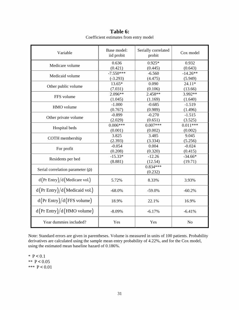
In Table 6, we present estimates of our entry model, using three specifications: the base model
from (5) which is an iid probit, a serially correlated probit based on (6) and the Cox specification from
(7). The relative magnitudes of the coefficients are consistent across the different specifications. We find,
for the major payers, the average returns over our study period are the most generous for FFS, followed
by Medicare, HMO and Medicaid. Average Medicare returns over the period are positive, small, but
statistically significant only in the serially correlated probit specification. FFS returns are always
significantly positive and appear to be roughly three times that of Medicare. HMO returns are slightly
below zero and never statistically significant. Medicaid consistently pays below average variable cost,
with a return that is estimated to be roughly 3 times the magnitude for that of FFS, but with the opposite
sign, and is significant except in the serially correlated probit specification.
The coefficient on serial correlation in the serially correlated probit, ρ, is found to be 0.834 and
significant. However, the coefficients are similar in magnitude and significance across the two probit
specifications. We are not aware of any direct way of testing the probit models against the Cox model
and the magnitude of the coefficients are not directly comparable across the specifications. However, we
can compare the magnitudes by examining the derivative of the probability of entry with respect to a
16 The dependent variable excludes patients omitted from the sample due to the data problems noted in Section 3.

18
change in volume by payer, evaluated for a hospital at the sample mean probability of entry.17 Table 6
reports that these magnitudes are very consistent across the specifications for the four key payer types.
Hence, we focus on the iid probit for the subsequent results.
Our findings are consistent with those of Cutler and McClellan (1996), who find that HMO
penetration is inversely related to entry at the state level. Our analysis demonstrates that the inverse
relation between HMO penetration and entry is not because HMOs pay below variable costs but because
they pay less than other payers.
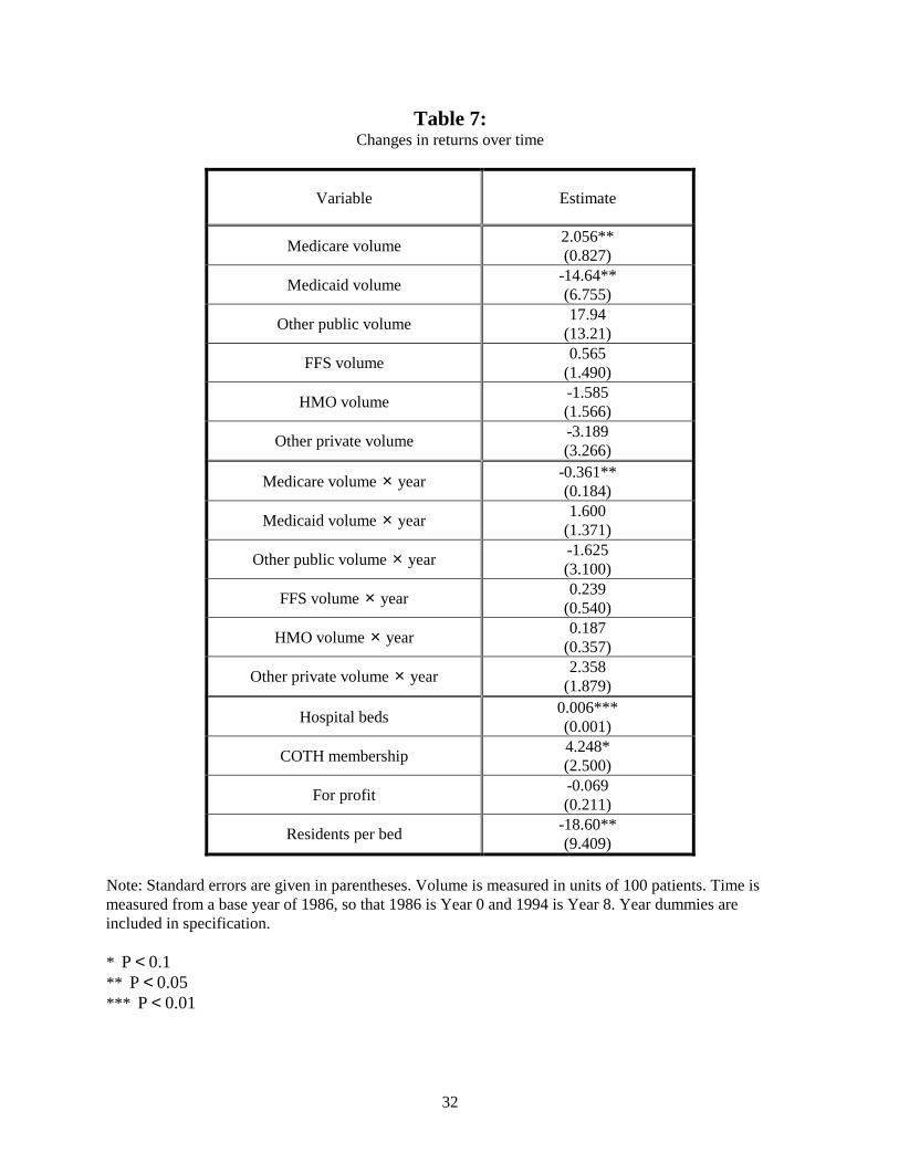
By interacting volume with a time trend, we find evidence that returns for Medicare are
decreasing over our sample period, and that the decrease is statistically significant (Table 7). The results
show that in 1986, the start of our sample period, Medicare reimbursed with a similar return to the FFS
return from Table 6 (β = 2.056 vs. 2.096), while by 1994, returns for Medicare are negative, (β = -
0.832).18 The small Medicare coefficient in Table 6 reflects the average of high early period returns and
low or negative later period returns. The drop in returns for Medicare is consistent with published
Medicare returns, which show a similar decrease in overall hospital reimbursement rates over our sample
period.19 In contrast to the Medicare results, we do not find any other statistically significant time
variation in returns. Medicaid returns are shown to be increasing during our sample period, though the
increase is not statistically significant at the .10 level.
The estimates presented above assume that average returns are invariant to market competition.
We explore this hypothesis by interacting the predicted volume estimates for each hospital with a
Herfindahl for that hospital.20 The Herfindahl is based on share of CABG admissions for hospitals within
a 30-kilometer radius of the hospital in question.21
Separate Herfindahl indices are created each year for
each hospital and are not payer specific.
17 For the Cox specification, this should be interpreted as the derivative of the cumulative probability of entry over aone year period conditional on no entry at the start of the period.18 Recall all patients over 65 were recoded as Medicare patients even though some were enrolled in HMOs. Thisrecoding addressed data problems and conceptual issues associated with Medicare HMOs. Without the recoding thedeclining trend in Medicare returns, which we know from secondary sources existed, disappears. Thus we trust theresults with the recoded data.19 Prospective Payment Assessment Commission (1995).20 Returns would also be affected by competition in the insurance market (including among HMOs). We do notmeasure this competition.21 Competition may influence returns for Medicare and Medicaid patients if there is quality competition, whichincreases costs.

19
The results suggest that HMO returns increase with decreased competition (or equivalently, with
increased Herfindahl) (Table 8). None of the other interactions with competition are statistically
significant. HMO returns approximate FFS returns from Table 6 in markets with a Herfindahl of .616.
HMO returns approximate 0 in markets with a Herfindahl equivalent to .398 (approximately 2.5 equal
sized hospitals). This is close to the mean Herfindahl in our sample (.395). Bresnahan and Reiss (1991)
also report that most of the gains to competition are achieved with relatively few providers, and our
estimates suggest competition in the market for HMO patients is even more vigorous. Given the amount
of search in the HMO market, this is not surprising. In contrast, the statistically insignificant coefficients
on the FFS and Medicare interactions suggest that these returns are not much affected by competition.
4.3 Sensitivity analysis
We examine the sensitivity of our results to three possible effects: unobserved market traits that
are correlated with both entry and payer mix, demand expansion from entry, and the endogeneity of
volume.
First, note that the results presented above are partly identified on the basis of the payer mix of
the population in the geographic area surrounding the potential entrants. If unobserved market
characteristics are correlated with payer mix, the results may bias our estimates of returns. For example,
assume that hospitals in areas with a large number of Medicaid recipients have a difficult time attracting
cardiac surgeons or that high Medicaid volume is correlated with a high percentage of uninsured.22 We
will predict a high Medicaid volume for potential entrants in these areas and a low probability of entry.
This will lead to an inference of low or negative margins. To test for such market specific effects, we re-
estimate the entry model with additional explanatory variables that measure the mean payer mix for all
admissions in the hospital’s market.23 For this specification, the identification of the returns will come
from the level of competition for different types of patients.
These estimates yield very similar predictions to the base model, except that the Medicaid market
share is no longer significant, and the absolute value of the point estimate on Medicaid returns drops by
22 Uninsured patients are included in the ‘other private’ category, but if the proportion of uninsured in that categoryvaries with Medicaid enrollment there may still be a measurement issue.23 We define the market to be the set of people who live within 120 kilometers of the hospital who were dischargedfrom a hospital in California.

20
about 35% (Table 6 column 1 vs. Table 9, column 1). Since Medicaid market share is the omitted
category, the positive signs on all the other coefficients suggest that areas with high Medicaid penetration
are relatively unattractive. In contrast, the estimates suggest that areas with high HMO penetration and
high Medicare penetration are attractive for entrants, even controlling for predicted volume. Perhaps it is
easy to attract physicians to these areas, lowering the fixed costs of entry.
A second issue related to our base results is that we have not allowed for the possibility that new
entrants may expand the demand for CABG surgery. Specifically, evidence suggests that aggregate
volume will rise with entry simply because of reduced distance from patients to CABG providers (Cutler
and McClellan, 1996). To explore the sensitivity of our results to potential demand expansion, we
include estimates of the percentage of ischemic heart disease admissions in each hospital’s market area
that received CABG.24 A higher percentage would suggest a lower potential for demand expansion and
thus a lower probability of entry. Therefore a negative sign on the CABG rate is consistent with the
ability for significant demand expansion for that payer.
The results display the same pattern of results as the base analysis, although some of the
coefficients change in magnitude. Most notably, the estimated FFS returns rise by about 70% in this
specification (Table 6 column 1 vs. Table 9, column 2), which strengthens our earlier finding that FFS
payers generate a positive return. This is supported by the large and negative, though insignificant,
coefficient on the FFS CABG rate which suggests that entry is more likely when inducement
opportunities are high (low CABG rate). In contrast, the large, positive and significant coefficient on the
Medicaid CABG rates suggests that entrants are more likely if there is little room to expand CABG
surgery for Medicaid patients. This supports the earlier finding that Medicaid does not provide sufficient
returns because it is consistent with the hypothesis that hospitals do not want to enter areas where they
may be forced to provide services to patients whose insurers do not provide sufficient returns.
Finally, the predicted volume that we use in our entry model is potentially endogenous because it
is based on our assumption of rational expectations regarding competitive interactions. Specifically, in
our base analysis, we calculate predicted volume for any potential entrant using as the choice set all
hospitals that actually provide CABG services in the year of entry. Thus, the predicted volume for any
24 Following Langa and Sussman (1993), we use the following ICD-9 diagnosis codes for ischemic heart disease:410.xx, 411.1, 411.8, 413.xx, 414.0x, 414.8x, and 414.9x.

21
potential entrant reflects the unobserved factors driving competitors to enter. Because we assume the
potential entrant observes these factors, there is a correlation between entrants’ predicted volumes and
the unobserved component of their entry decisions.25
To explore the sensitivity of our results to this endogeneity we estimate a linear probability
model of entry using IV techniques. Our instruments consist of predicted volume calculated assuming
only the potential entrant and incumbents were in the market. Any unobserved factors that influence
competitors to enter are not reflected in this instrument, eliminating the cause of the endogeneity. The
instruments are essentially functions of the characteristics of the competing firms, aggregated in a
manner that emphasizes the proximity of the competitors to the potential entrant in product space.26
We find that the use of instruments yields conclusions similar to those derived from our primary
analysis (Table 9, column 3).27 While it is not possible to directly compare the IV coefficients to the
coefficients from our base model which assumed the hazard function was based on a normal distribution
of the entry equation error, the signs and significance of all the coefficients of interest remain the same.
Moreover, a Hausman test of the IV model against a linear probability model fails to reject the
consistency of the non-IV model (P=0.50).
5. Implications and Conclusions
Estimating the returns by payer type that hospitals receive from the provision of high-technology
medical services is important. There has been substantial concern among policy makers regarding ‘over
diffusion’ of expensive medical technologies such as CABG, which could be driven by excess returns to
the provision of such services. Yet, accounting complexities and case-mix variation make direct
assessment of returns difficult. We rely on entry decisions, together with a structural model of entry, to
infer returns. The analysis not only confirms widely held opinions about the relative generosity of
payments, but also presents new evidence regarding the magnitude of returns, and the changes in these
returns over time and across different levels of competition. 25 Berry (1992) focuses on this issue in an examination of entry among airlines.26 Similarly, Frank and Salkever (1991) use characteristics of competing hospitals to instrument for endogenousselection into insurance, in a study of the provision of charity care.27 The similar results are in spite of the fact that a Hausman test suggests the presence of endogeneity in our volumecoefficients.

22
Our analysis reveals that Medicare returns for CABG have followed the same pattern of
aggregate Medicare returns: generous in the mid 1980s, but approximating zero by the early/mid 1990s.
Only Medicare returns were sensitive to time. Throughout our study period, HMOs appear to reimburse
hospitals at approximately average variable costs. This result is consistent with models of strong price
sensitive search by HMOs and the absence of hospital market power in this payer segment. Although our
results suggest that HMOs are not contributing to fixed costs, they are not paying substantially below
variable costs as some of their opponents contend. In contrast, Medicaid payments seem below variable
costs. Commercial and BCBS payers pay the most generous returns, which appear to have been relatively
constant over time. By the end of study period, only these payers are contributing to fixed costs. Finally,
our results suggest that HMO returns (and only HMO returns) are particularly sensitive to competition
among CABG providers. We find that it takes between two and three CABG providers in the market to
drive returns from HMOs to zero.
Most experts predict continued growth in enrollment in HMOs and in other plans which shop for
hospitals based on price. Our results indicate that this will mean fewer payers that contribute to fixed
costs. Thus, future entry into CABG is likely to be much slower and exit from the market is possible.
Mergers by hospitals to gain market power in their dealings with HMOs are also likely. In this scenario,
returns from HMOs and other strongly managed plans are likely to grow. This implies that cost savings
achieved by HMOs through efficient purchasing may diminish.
Moreover, to the extent that our results are generalizable to other services, they suggest that there
will be a slowdown in the rate of entry for other high-technology services in the hospital sector. Although
we cannot assess the health consequences of use, which is necessary to quantify whether there is ‘over-
diffusion’, our results suggest that hospitals continue to have the incentive to encourage CABG
procedures for FFS patients at the margin. In contrast, HMOs do not give hospitals this incentive and by
the end of our study period, Medicare payment rates have also removed the hospital incentive to provide
this surgery. The lower payment by Medicaid suggests an incentive for lower utilization, implying that
these patients will likely face continued access difficulties.28
28 Langa and Sussman (1993) report that during the mid 1980s, rates of revascularization (CABG and PTCA) grewthe least in the Medicaid population.

23
While our estimation appears to give reasonable results, there are several modeling and
econometric specification issues that arise. First, we make the restrictive assumption that, holding the
Herfindahl constant, average returns are fixed for a given payer type. Second, we have treated our
predicted volumes as not having any measurement error, even though this may occur for a finite sample
of patients. Third, we have not incorporated dynamics into our return function.
We feel that this work makes two methodological contributions to the general health economics
and industrial organization literature. First, this paper shows how to construct an entry model where
markets are endogenously determined. Specifically, our method uses a patient flow model to base market
definitions on an estimated demand structure. In contrast, existing entry papers have used pre-determined
geographic market definitions. This is potentially problematic because these pre-determined markets are
relatively inflexible in their ability to control for differing degrees of product differentiation created
largely by differential distances between competitors within the market.
Second, we feel that this paper lends credence to the general modeling approach of assuming
positive returns from entry, and using this to infer structural parameters. Other authors have either
focused on different motives for hospital entry into high-technology services [e.g. the medical arms race;
see Luft et al. (1986) and Dranove, Shanley and Simon (1992)] or have been more agnostic regarding the
motives for entry [e.g. Cutler and McClellan (1996)]. We believe that our emphasis on returns is justified
because our results are both consistent with economic theories and with accounting data. Other models
would have to explain such features of the data such as why only Medicare returns decline significantly
over time and why only HMO returns respond significantly to competition. Thus, our results suggest that
it is a valid and useful endeavor to estimate entry models for other industries in order to infer
fundamental parameters that are of economic interest.

24
References
Allison, P.D., 1995. Survival Analysis Using the SAS System : A Practical Guide. Cary NC: SASInstitute.
Baker, L.C., Wheeler, S.K., 1998. Managed Care and Technology Diffusion: The case of MRI. HealthAffairs 17(5), 195-207
Berry, S.T., 1994. Estimating Discrete-Choice Models of Product Differentiation. RAND Journal ofEconomics 25, 242-262.
Berry, S.T., 1992. Estimation of a Model of Entry in the Airline Industry. Econometrica 60(4), 889-917
Bresnahan, T., Reiss, P., 1991. Entry and Competition in Concentrated Markets. Journal of PoliticalEconomy 99(5), 977-1009.
Burns, L.R., Wholey, D.R., 1992. The Impact of Physician Characteristics in Conditional Choice Modelsfor Hospital. Journal of Health Economics 11(1), 43-62.
Chernew, M., Scanlon, D., Hayward, R., 1998. Insurance Type and Choice of Hospital for Open HeartSurgery. Health Services Research 33(3), 447-466.
Cutler, D.M., McClellan, M., 1996. The Determinants of Technological Change in Heart AttackTreatment. NBER Working Paper Series. Working Paper 5751.
Dranove, D., Shanley, M., Simon, C., 1992. Is Hospital Competition Wasteful? RAND Journal ofEconomics 23(2), 247-262.
D’Agostino, R.B., Lee M.L., Belanger A.J., Cupples, L.A., Anderson K., W.B., Kannel, W.B., 1990.Relation of Pooled Logistic Regression to Time Dependent Cox Regression Analysis: TheFramingham Heart Study. Statistics in Medicine 9(12), 1501-1515.
Frank, R., Salkever, D.S., 1991. The Supply of Charity Services by Non-Profit Hospitals: Motives andMarket Structure. RAND Journal of Economics 22(3), 430 – 444.
Garnick, D.W., Lichtenberg, E., Phibbs, C.S., Luft, H.S., Peltzman, D.J., McPhee., S.J., 1989. TheSensitivity of Conditional Choice Models for Hospital Care to Estimation Technique. Journal ofHealth Economics 8, 377-397.
Geweke, J., 1989. Bayesian Inference in Econometric Models Using Monte Carlo Integration.Econometrica 57, 1317-39.
Hadley, J., Feder, J., 1985. Hospital cost shifting and care for the uninsured. Health Affairs 4(3), 67-80.
Hajivassiliou, V.A., McFadden, D., Ruud, P., 1996. Simulation of Multivariate Normal RectangleProbabilities and Their Derivatives: Theoretical and Computational Results. Journal ofEconometrics 72, 85-134.

25
Keane, M., 1994. A Computationally Practical Simulation Estimator for Panel Data. Econometrica 62,95-116.
Langa, K.M., Sussman, E.J., 1993. The effect of cost-containment policies on rates of coronaryrevascularization in California. New England Journal of Medicine 329(24), 1784-9.
Luft, H.S., Garnick, D.W., Mark, D.H., Peltzman, D.J., Phibbs, C.S., Lichtenberg, E., McPhee, S.J.,1990. Does Quality Influence Choice of Hospital? Journal of The American Medical Association263(21), 2899-2906.
Luft, H.S., Robinson, J.C., Garnick, D.W., Maerki, S.C., McPhee, S.J., 1986. The Role of SpecializedClinical Services in Competition Among Hospitals. Inquiry 23, 83-94.
McFadden, D., 1973. Conditional Logit Analysis of Qualitative Choice Behavior, in: Zarembka P,Frontiers in Econometrics, New York: Academic Press.
McFadden, D., 1974. The Measurement of Urban Travel Demand. Journal of Public Economics 3, 303-328.
Morrisey, M., 1995. Movies and Myths: Hospital Cost Shifting. Business Economics 30 22 – 25.
National Center for Health Statistics, 1997. National Hospital Discharge Survey. Detailed Diagnoses andProcedures. 1994. Vital Health Statistics 13(127).
National Center for Health Statistics, 1986. National Hospital Discharge Survey. Detailed Diagnoses andProcedures for Patients Discharged from Short Stay Hospitals. United States, 1984. Vital HealthStatistics 13(86).
Phibbs, C.S., Mark, D.H., Luft, H.S., Peltzman-Rennie, D.J., Garnick, D.W., Lichtenberg, E., McPhee,S.J., 1993. Choice of Hospital for Delivery: A Comparison of High-Risk and Low-Risk Women.Health Services Research 28(2), 201-222.
Prospective Payment Assessment Commission, 1995. Medicare and the American Health Care SystemReport to Congress.
Spetz, J., Baker, L.C., 1999. Has Managed Care Affected the Availability of Medical Technology? SanFrancisco, CA. Public Policy Institute of California.
26
Table 1:CABG entry by year
Year Incumbents Potential entrants EntrantsPercent of
potential entrantsthat enter
1985 84 142 1 1%
1986 85 143 8 6%
1987 93 136 10 7%
1988 103 125 7 6%
1989 110 120 7 6%
1990 116 114 2 2%
1991 117 111 4 4%
1992 119 108 2 2%
1993 121 107 4 4%
1994 125 102 1 1%
Total 1073 1208 46 4%
Unique Hospitals 129 154 46 30%
Note: Between 1989 and 1991 there were a total of 4 exits, which is why the number of incumbentsbetween 1990 to 1992 does not match the number of entrants plus incumbents in the previous year.
27
Table 2:Descriptive statistics on hospitals
‘In’ CABG Potential entrants Entrants
Beds 342(206)
180(88)
247(87)
CABG Distancetraveled (KM)
18.50(12.2)
14.02(9.7)
For profit 13% 27% 20%
Private not-for-profit 84% 64% 78%
Public 3% 9% 2%
COTH Member 15% 3% 2%
Residents per bed 0.07(0.2)
0.03(0.1)
0.01(0.0)
Non-cardiac volumeper year
15,464(9561)
8157(5470)
11,300(4723)
Cath volume per year 646(405)
83(118)
292(140)
PTCA volume peryear
245(201)
53(56)
Medicare 156(145)
43(29)
Medicaid 16(25)
3(9)
FFS/commercial
51(50)
21(19)
HMO 40(76)
7(9)
Other public 5(9)
1(2)
Other private 10(17)
2(3)C
AB
G v
olum
e pe
r yea
r
Total 278(244)
77(47)
N 1034 1066 45
Note: Each cell indicates the mean value, with the standard deviation in parentheses.

28
Table 3:Coefficient estimates from patient flow model
Coefficient type Mean Min Max Positive Negative
Beds × 100 -0.012 -0.608 0.471 28 26
Public -0.866 -3.576 2.044 15 39
For profit -0.352 -1.403 0.208 7 47
COTH 0.332 -0.817 2.262 36 18
Residents per bed 0.248 -2.342 3.197 31 23
( )ln Dist 1+ 0.017 -0.323 0.795 23 31
( ) 2ln Dist 1+� �� � -0.331 -0.464 -0.250 0 54
Lag cath volume 0.010 -5.923 4.142 30 24
Lag PTCA volume 1.466 -3.160 11.17 38 16
2 Lag cath volume 0.237 -2.239 5.980 31 23
2 Lag PTCA volume 0.110 -6.057 8.986 23 31
2 Lag-CABG volume 0.152 -5.843 6.485 24 30
Lag CABG vol. Medicare 0.222 -0.183 1.017 49 5
Lag CABG vol. Medicaid 0.781 -1.151 6.104 44 10
Lag CABG vol. Other pub. 1.063 -3.912 9.964 36 18
Lag CABG vol. FFS 0.030 -1.222 1.132 33 21
Lag CABG vol. HMO 0.116 -1.208 1.835 34 20
Lag CABG vol. Other priv. 0.559 -3.663 5.649 36 18
Non-heart vol. Medicare -0.208 -2.858 3.367 24 30
Non-heart vol. Medicaid -0.182 -3.086 0.944 21 33
Non-heart vol. Other pub. 0.675 -6.682 12.15 29 25
Non-heart vol. FFS 0.118 -1.896 2.147 30 24
Non-heart vol. HMO 0.022 -2.394 2.147 25 29
Non-heart vol. Other priv. -0.2869 -4.476 4.612 21 33
Percent own race 1.521 0.836 3.614 54 0
Note: Each row pertains to 54 estimated coefficients, corresponding to 9 years of data and six payergroups. Volume is measured in units of 100 patients.

29
Table 4:Correlation between actual 1994 volume and predicted 1994 volume
Predicted 1994 volume based on coefficients from:Actual1994
Keptfrom
199429 1994 1993 1992 1991 1990 1989
Actual 1994 1.00
Kept from 1994 1.00 1.00
1994 0.97 0.97 1.00
1993 0.85 0.86 0.89 1.00
1992 0.87 0.88 0.92 0.90 1.00
1991 0.81 0.83 0.86 0.82 0.96 1.00
1990 0.80 0.81 0.83 0.82 0.91 0.91 1.00
Pred
icte
d 19
94 v
olum
e ba
sed
on c
oeff
icie
nts f
rom
1989 0.84 0.84 0.88 0.86 0.89 0.84 0.93 1.00
Note: An observation is a hospital that is ‘in’ the CABG market × payer type.
29 Patients were omitted if they had missing distance data, traveled further than 120 kilometers, or received care athospitals with too little volume to be considered ‘in’ the CABG market.

30
Table 5:Bias in predicted volume for actual entrants
Regressor Estimate
Constant 2.048***(0.276)
Predicted volume 0.960***(0.003)
Pred. Volume × Medicare × entry at t –0.394***(0.042)
Pred. Volume × Medicaid× entry at t –0.543(0.658)
Pred. Volume × other public × entry at t –1.388(1.381)
Pred. Volume × FFS × entry at t –0.261*(0.097)
Pred. Volume × HMO × entry at t –0.546*(0.209)
Pred. volume × other private × entry at t –0.582(0.031)
Pred. volume × Medicare × entry at t–1 –0.059*(0.031)
Pred. volume × Medicaid× entry at t–1 0.044(0.426)
Pred. volume × other public × entry at t–1 –0.517(1.086)
Pred. volume × FFS × entry at t–1 –0.051(0.068)
Pred. volume × HMO × entry at t–1 –0.204(0.154)
Pred. volume × other private × entry at t–1 –0.303(0.519)
2R 0.95
Note: The dependent variable is the actual kept volume. An observation is a hospital that is ‘in’ theCABG market × payer type × year. Standard errors are given in parentheses.
* P 0.1<** P 0.05<*** P 0.01<
31
Table 6:Coefficient estimates from entry model
Variable Base model:iid probit
Serially correlatedprobit Cox model
Medicare volume 0.636(0.421)
0.925*(0.445)
0.932(0.643)
Medicaid volume -7.550***(-3.293)
-6.560(4.475)
-14.26**(5.949)
Other public volume 13.65*(7.031)
0.090(0.106)
24.11*(13.66)
FFS volume 2.096**(1.045)
2.458**(1.169)
3.992**(1.640)
HMO volume -1.000(0.767)
-0.685(0.989)
-1.519(1.496)
Other private volume -0.899(2.029)
-0.270(0.651)
-1.515(3.525)
Hospital beds 0.006***(0.001)
0.007***(0.002)
0.011***(0.002)
COTH membership 3.825(2.393)
3.485(3.334)
9.045(5.256)
For profit -0.054(0.208)
0.004(0.320)
-0.024(0.415)
Residents per bed -15.33*(8.881)
-12.26(12.54)
-34.66*(19.71)
Serial correlation parameter (ρ) 0.834***(0.232)
( ) ( )d Pr Entry d Medicare vol. 5.72% 8.33% 3.93%
( ) ( )d Pr Entry d Medicaid vol. -68.0% -59.0% -60.2%
( ) ( )d Pr Entry d FFS volume 18.9% 22.1% 16.9%
( ) ( )d Pr Entry d HMO volume -8.09% -6.17% -6.41%
Year dummies included? Yes Yes No
Note: Standard errors are given in parentheses. Volume is measured in units of 100 patients. Probabilityderivatives are calculated using the sample mean entry probability of 4.22%, and for the Cox model,using the estimated mean baseline hazard of 0.186%.
* P 0.1<** P 0.05<*** P 0.01<
32
Table 7:Changes in returns over time
Variable Estimate
Medicare volume 2.056**(0.827)
Medicaid volume -14.64**(6.755)
Other public volume 17.94(13.21)
FFS volume 0.565(1.490)
HMO volume -1.585(1.566)
Other private volume -3.189(3.266)
Medicare volume × year -0.361**(0.184)
Medicaid volume × year 1.600(1.371)
Other public volume × year -1.625(3.100)
FFS volume × year 0.239(0.540)
HMO volume × year 0.187(0.357)
Other private volume × year 2.358(1.879)
Hospital beds 0.006***(0.001)
COTH membership 4.248*(2.500)
For profit -0.069(0.211)
Residents per bed -18.60**(9.409)
Note: Standard errors are given in parentheses. Volume is measured in units of 100 patients. Time ismeasured from a base year of 1986, so that 1986 is Year 0 and 1994 is Year 8. Year dummies areincluded in specification.
* P 0.1<** P 0.05<*** P 0.01<

33
Table 8:Impact of competition on returns
Variable Estimate
Medicare volume 1.358(0.839)
Medicaid volume -2.414(7.102)
Other public volume 28.74**(14.04)
FFS volume 1.421(1.499)
HMO volume -3.833*(2.061)
Other private volume -6.501(4.127)
Medicare volume × Herfindahl -1.690(1.321)
Medicaid volume × Herfindahl -6.822(9.060)
Other public volume × Herfindahl -29.79(21.60)
FFS volume × Herfindahl 0.890(2.872)
HMO volume × Herfindahl 9.629*(5.428)
Other private volume × Herfindahl 27.57(12.75)
Hospital beds 0.007***(0.001)
COTH membership 4.753*(2.512)
For profit 0.006(0.224)
Residents per bed -17.99*(9.358)
Note: Standard errors are given in parentheses. Volume is measured in units of 100 patients. Yeardummies are included in specification.
* P 0.1<** P 0.05<*** P 0.01<

34
Table 9:Sensitivity analysis
Variable Including payermix
Including CABG.rate
Instrumentalvariables
Medicare volume 0.493(0.452)
0.335(0.455)
0.046(0.037)
Medicaid volume -4.920(4.061)
-7.580*(0.413)
-0.541**(0.192)
Other public volume 6.599(7.898)
9.156(8.279)
0.734(0.555)
FFS volume 3.704***(1.182)
3.606***(1.173)
0.309***(0.093)
HMO volume -0.879(0.810)
-0.553(0.758)
-0.059**(0.024)
Other private volume -0.490(2.282)
-0.969(2.456)
-0.140(0.145)
Medicare market share 10.58*(5.888)
Other public market share 41.99***(13.49)
FFS market share 5.718(5.847)
HMO market share 10.49**(4.739)
Other private market share 8.114(13.78)
Medicare CABG rate 3.512(14.08)
Medicaid CABG rate 18.16**(8.042)
Other public CABG rate 5.977***(2.257)
FFS CABG rate -15.73(10.23)
HMO CABG rate 0.547(4.522)
Other private CABG rate 6.689(5.131)
Note: Standard errors are given in parentheses. Volume is measured in units of 100 patients. Yeardummies, Beds, COTH, For-profit and Residents per bed are included in all specifications.
* P 0.1<** P 0.05<*** P 0.01<