Paving the Bridge between Academia and … the Bridge between Academia and Operations for Orbital Debris ... which allows for greater precision and the ability ... Then the Pc inequalities

Paving the Bridge between Academia and Operations for Orbital Debris Risk Mitigation

Mark A. Vincent

Raytheon

ABSTRACT

A computer program named PC4 has been created to produce the confidence levels that future Probability of

Collision (Pc) will not exceed chosen thresholds. Its results compared favorably to those from an earlier spreadsheet

version using the same algorithms. Insights into the bounding values of both current and future Pc values were

obtained. The need for state covariance scaling and improved modeling of solar activity/atmospheric density is

presented. The recommended post-maneuver thresholds for maneuver planning are also presented.

1. INTRODUCTION

How to manage the risk from orbital debris continues to be a vexing problem for operators of Earth-orbiting

satellites. Further analysis has been performed to address the issues raised in a previous paper [1]. The three main

topics presented here are Probability of Collision (Pc) Forecasting, Covariance Scaling and Post-maneuver Pc

Thresholds.

The previous paper (ibid) explained how the Pc forecasting was done in the manner of a spreadsheet. The same

algorithms were coded into a MATLAB program named PC4, which allows for greater precision and the ability to

do more rapid investigations. One interesting result from the initial investigations was a regression back to a better

understanding of the limits and implications of the current Pc calculation. Another useful application was doing spot

check comparisons to the formulas and tables of Chan’s preeminent textbook [2] on the subject.

Covariance Scaling has garnered attention recently once it was realized that the predicted covariances used in Pc

calculations did not really represent the true uncertainty in the propagated states of the bodies involved. Note this is

not due to the formulation and propagation of the covariance matrix, a subject that generated a lot of academic

interest and publications in the recent years. Rather the issue is the uncertainty in the force modeling, mainly

atmospheric drag, which dominates the need for scaling. Techniques such as consider parameterization and process

noise have been well documented but the extent to which, and how, empirical data must be used to implement these

techniques has been addressed only relatively recently. A further complication is encountered when a maneuver is

involved in the propagation.

The previous paper [1] briefly mentioned the issue of post-maneuver Pc thresholds. Subsequent implementation of

them for the Orbiting Carbon Observatory-2 (OCO-2) indicated that several different thresholds were needed. For

example, Risk Mitigation Maneuvers (RMMs), which have limited flexibility in their magnitude and time of

occurrence, should have less strict requirements compared to maneuvers that can be postponed. The timing between

the maneuver and the conjunction(s) being considered also proved to be a delineating factor in the choice of

thresholds.

2. PROBABILITY OF COLLISION FORECASTING

Background

The basic premise of Pc forecasting is to use the current state knowledge and a prediction of the amount of

uncertainty at a future epoch to give a Confidence Level (CL) of the Pc at that later epoch. The term confidence level

is used to distinguish it from Pc values though actually it is in itself a probability. Specifically CL can be thought of

as the probability that Pcf < PcT where Pcf is the range of possible future Pc’s and PcT is the Pc threshold of interest.

Also note that PcT can be a specific value, such as the threshold when a maneuver must be performed or simply the

current Pc value (i.e. what is the confidence level that future Pc will not be worse than the present situation?). The

approximations and caveats of using the tool are explained in the following.

Copyright © 2016 Advanced Maui Optical and Space Surveillance Technologies Conference (AMOS) – www.amostech.com

Comparison of the Assumptions used in the Spreadsheet and PC4

The major assumption used in the forecasting tool and actually throughout most estimation theory is that the

probability distributions functions (PDFs) involved are zero-mean Gaussian distributions. Further, the estimates of

the covariance, in this case at the Time of Closest Approach (TCA), have to be representative of the truth, or not

only is the current Pc estimate unreliable but the basis for using the forecasting tool is taken away. Biases need to be

removed and covariances scaled appropriately, as described in a later section.

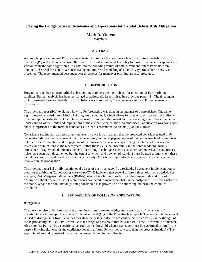
The “encounter plane” (sometimes called the b-plane) is perpendicular to the relative velocity between the primary

and secondary bodies of interest. At the TCA the positional vector from primary to secondary creates one axis called

the Miss Distance (MD) direction in the encounter plane. A vector which is perpendicular to it and also in the

encounter plane forms the second axis called here the Perpendicular Direction (PD).

The spreadsheet results that were created previously corresponded to about 50 bins in both the MD and PD

directions. The PC4 computer code allowed the number of bins to be specified by the user, and a quick trial

indicated that 200 bins in each direction provided enough precision in the results. However there is one caveat, the

spreadsheet changed the size of the bins so there were more bins near the center of the PDFs, In other words the bin

sized accounted for the higher probability density near the origin. The same could have been done for PC4 version

but the desired improvement in precision was obtained by just using a large number of bins, while the runtime was

kept almost instantaneous. Note the grid pattern shown in Fig. 1 is coarser than that used in either tool.

Fig. 1. Geometry of the Current and Future Probability Distributions

Another assumption used in both tools is that the major principle axis of both the current and future covariance

matrices is lined up in the Miss Distance direction. The assumption that the future covariance (red ellipses in Figure

1) can be predicted is further qualified that it must be known for any possible new position of the primary (P2). Thus

the fact that the current tools assume that one future covariance can be used for all possible values of P2 is certainly

a limitation that should be studied in the future if a forecasting tool is considered for operations.

The major principle axis of the covariance being in the MD direction of corresponds to the encounter plane being

nearly the local horizontal direction and the radial separation of the two orbits is small compared to the in-track and

cross-track components. This represents the majority of conjunction for objects in near-circular, low Earth orbits.

The counter-example of an overhead encounter is discussed in Chan [2], starting on Page 28.


Insight into Current Pc with Zero Miss Distances

One of the preliminary results of the PC4 tool was also seen in the spreadsheet tool, namely once the future

covariance was large enough the CL of exceeding a reasonable threshold went to 100.0%. This turns out to be

intuitively obvious but regressing and looking at the general Pc calculation is the first step. First, realize that the case

of having a zero miss distance has a higher Pc than any other miss distances for any given covariance. Colloquially,

this can be thought of as the Secondary (S) being at the “top of the mountain” represented by the point P1 in Figure

1. The isotropic case, that is, when uncertainty in the MD and PD are the same (i.e. MD = PD) is considered first.

Note that this is not a typical situation but is useful for discussing and plotting. Also it is worth mentioning that

Chan uses a change in coordinates to make general uncertainties isotropic so a series solution to the Rician integral

can be used to calculate Pc rather than the numerical methods used in this analysis.

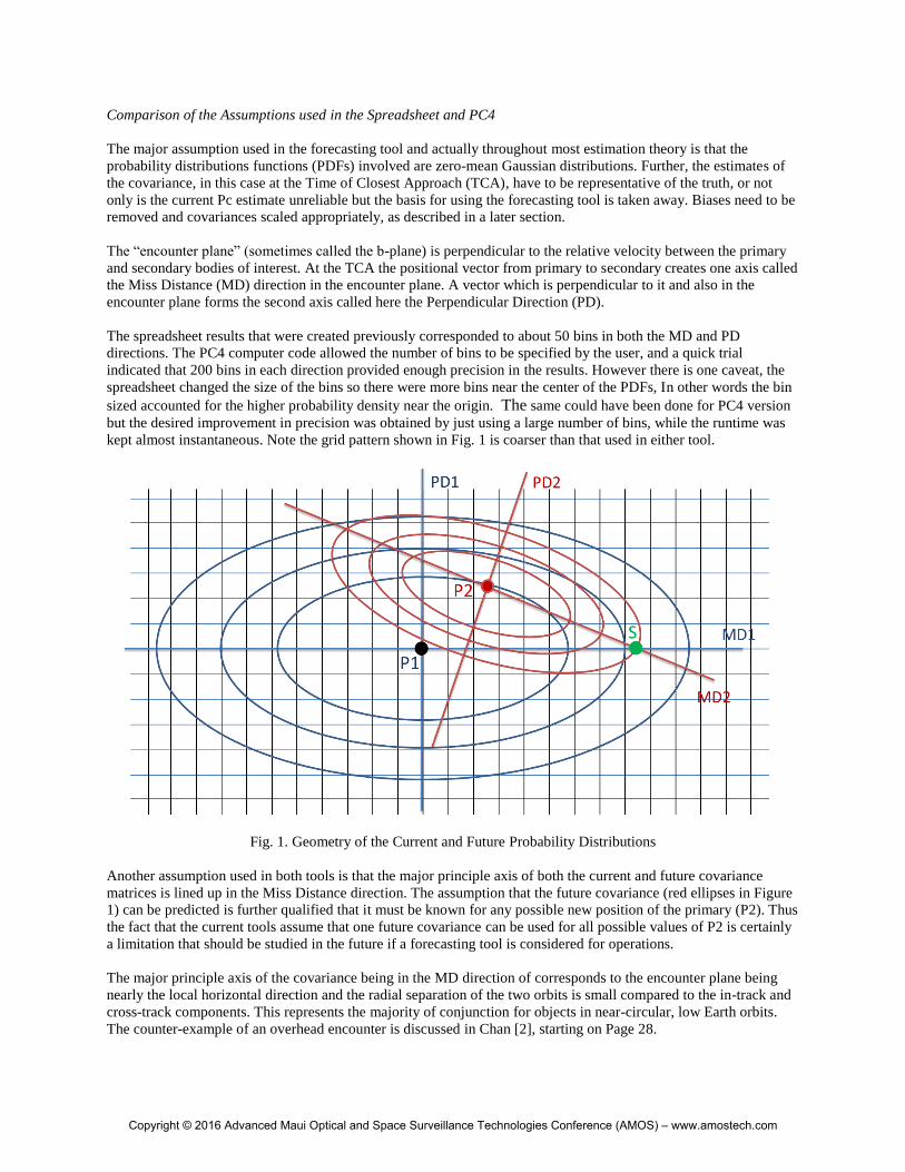
Fig. 2. Pc for Isotropic Standard Deviations with Zero Miss Distance and HBR = 6m

As seen in Fig. 2, if for example the is greater than 424 m then the Pc is less than 1x10-4

. This is not surprising

since it follows the “high covariance implies low Pc” maxim that is accepted, albeit with debate, in the literature [1,

3].

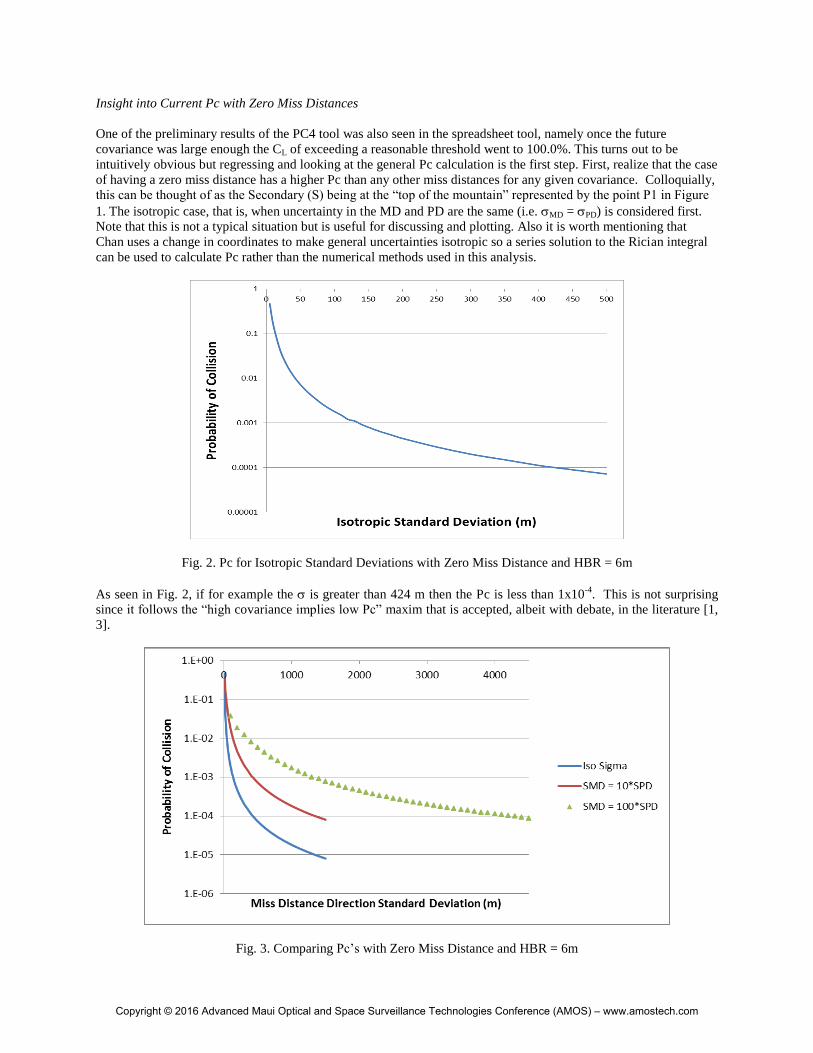
Fig. 3. Comparing Pc’s with Zero Miss Distance and HBR = 6m


Consider a typical ratio of MD being 10 times greater than PD , corresponding to an oblique conjunction with a

vertical encounter plane (see Chan [2], Table 2.3). This ratio reflects that typically the radial covariance component

is about 1/10 of the components in the horizontal plane directions. With this ratio, the results are shown in the red

line of Fig. 3. In this case, when MD and PD are close to 1300 and 130 m respectively the 1x10-4

threshold is

crossed.

Note for larger ’s that the PD dominates the Pc calculation and for even larger values, the Pc is proportional to the

PD since the blue line values are 10 times smaller than the red line ones. Also note the case for MD = 100* PD was

examined but not shown in the figure. In that case the Pc = 1x10-4

threshold was crossed when MD = 4200 and PD

= 42 m. This agrees with the previous statements about relationship between the two curves and also points out how

moderately high Pc values can exist with a large MD.

With the Fig. 3 curves in mind, the following describes the inference for the Pc forecasting: given the general case

depicted in Fig. 1, the largest future Pc will be when the future Miss Distance is zero, that is, when P2 is on top of S.

But then the curves in Fig. 2 and Fig. 3 correspond to the future 2MD and 2PD values. A simple example will be

used to illustrate this: independent of the current values, if the future isotropic is greater than 424 m (and HBR =

6m) then there is 100% confidence that the future Pc will be less than 1x10-4

.

The operational significance of having these 100% confidences is open for discussion. Consider the case when it is

Friday and the TCA is 6 days off and it is known that even with a new track over the weekend the resulting

uncertainty at the conjunction will correspond to a maximum Pc less than a comfortable threshold, then the staffing

for that weekend could be reduced. Two more controversial cases might be when either an impending solar storm or

a maneuver was going to increase the covariance enough so there was a 100% confidence of not crossing the chosen

threshold in the future. This would be even more controversial if the threshold was currently being crossed! These

two “added uncertainties” will be discussed later.

Hierarchy of Limiting Cases

There were some other limiting cases that were found to be interesting (and/or confusing) while performing the

above analysis. Switching notation a bit, let the Pc associated with the MD and PD standard deviations be

represented as P{MD, PD} and be a scale factor between 0 and 1 and as usual, the Miss Distance represented as

MD. Then the Pc inequalities that were discovered are:

P{MD, MD} ≤ P{MD/√2, MD/√2} ≤ P{MD, MD/√2} ≤ P{MD, 0}

This first inequality states for a fixed ratio of PD to MD (i.e. ) the maximum Pc occurs when the MD = √2*MD.

For the isotropic case ( = 1) this is the “Maximum Pc” presented by Alfano [3]. The second inequality indicates

that if PD is kept fixed then the maximum Pc is when MD = MD, this is related to Equation 11.11 of Chan [2] with

his = 0. Finally, the last inequality indicates that the greatest Pc of all occurs when PD = 0.

Again, a “visual” using Fig. 1 might help to put all this in perspective. If the blue curves represent the topographical

lines of a mountain, a person standing on the flank at S would be a maximum elevation for a fixed ratio when

√2*MD = MD. But with keeping the PD fixed, the person goes even higher when MD = MD and when PD goes to

zero he is standing at the ultimate height on an infinitesimally narrow ridge (which is also the univariate example).

Finally, note for the degenerate case when MD = 0, then all this discussion reduces to: the smaller the in either

direction the higher the Pc (or the steeper the sides of the mountain, the higher the peak, the volume of the mountain,

of course, remaining at unity).

Another interesting test case is to consider the results when the covariance at TCA associated with a future

observation is the same as the current estimate of the covariance at TCA. As Fig. 4 indicates, the future Pc then just

depends on what the future Miss Distance is. The green circle has radius equal to MD1 and thus being inside the

circle implies being closer to the secondary, that is MD2 < MD1 and thus Pc2 > Pc1.


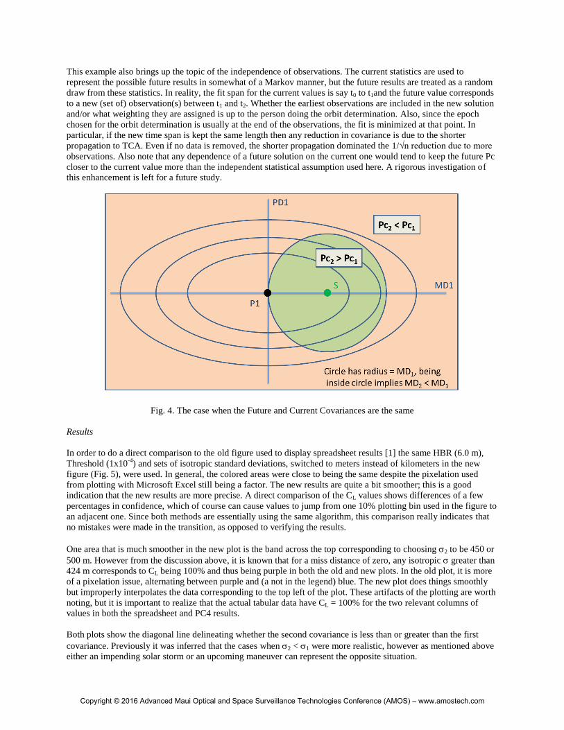
This example also brings up the topic of the independence of observations. The current statistics are used to

represent the possible future results in somewhat of a Markov manner, but the future results are treated as a random

draw from these statistics. In reality, the fit span for the current values is say t0 to t1and the future value corresponds

to a new (set of) observation(s) between t1 and t2. Whether the earliest observations are included in the new solution

and/or what weighting they are assigned is up to the person doing the orbit determination. Also, since the epoch

chosen for the orbit determination is usually at the end of the observations, the fit is minimized at that point. In

particular, if the new time span is kept the same length then any reduction in covariance is due to the shorter

propagation to TCA. Even if no data is removed, the shorter propagation dominated the 1/√n reduction due to more

observations. Also note that any dependence of a future solution on the current one would tend to keep the future Pc

closer to the current value more than the independent statistical assumption used here. A rigorous investigation of

this enhancement is left for a future study.

Fig. 4. The case when the Future and Current Covariances are the same

Results

In order to do a direct comparison to the old figure used to display spreadsheet results [1] the same HBR (6.0 m),

Threshold (1x10-4

) and sets of isotropic standard deviations, switched to meters instead of kilometers in the new

figure (Fig. 5), were used. In general, the colored areas were close to being the same despite the pixelation used

from plotting with Microsoft Excel still being a factor. The new results are quite a bit smoother; this is a good

indication that the new results are more precise. A direct comparison of the CL values shows differences of a few

percentages in confidence, which of course can cause values to jump from one 10% plotting bin used in the figure to

an adjacent one. Since both methods are essentially using the same algorithm, this comparison really indicates that

no mistakes were made in the transition, as opposed to verifying the results.

One area that is much smoother in the new plot is the band across the top corresponding to choosing 2 to be 450 or

500 m. However from the discussion above, it is known that for a miss distance of zero, any isotropic greater than

424 m corresponds to CL being 100% and thus being purple in both the old and new plots. In the old plot, it is more

of a pixelation issue, alternating between purple and (a not in the legend) blue. The new plot does things smoothly

but improperly interpolates the data corresponding to the top left of the plot. These artifacts of the plotting are worth

noting, but it is important to realize that the actual tabular data have CL = 100% for the two relevant columns of

values in both the spreadsheet and PC4 results.

Both plots show the diagonal line delineating whether the second covariance is less than or greater than the first

covariance. Previously it was inferred that the cases when 2 < 1 were more realistic, however as mentioned above

either an impending solar storm or an upcoming maneuver can represent the opposite situation.


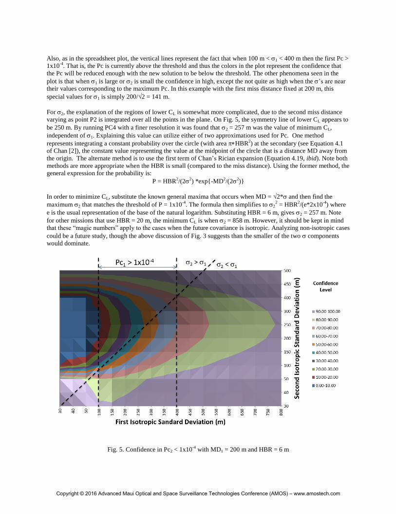
Also, as in the spreadsheet plot, the vertical lines represent the fact that when 100 m < 1 < 400 m then the first Pc >

1x10-4

. That is, the Pc is currently above the threshold and thus the colors in the plot represent the confidence that

the Pc will be reduced enough with the new solution to be below the threshold. The other phenomena seen in the

plot is that when 1 is large or 2 is small the confidence in high, except the not quite as high when the ’s are near

their values corresponding to the maximum Pc. In this example with the first miss distance fixed at 200 m, this

special values for 1 is simply 200/√2 = 141 m.

For 2, the explanation of the regions of lower CL is somewhat more complicated, due to the second miss distance

varying as point P2 is integrated over all the points in the plane. On Fig. 5, the symmetry line of lower CL appears to

be 250 m. By running PC4 with a finer resolution it was found that 2 = 257 m was the value of minimum CL,

independent of 1. Explaining this value can utilize either of two approximations used for Pc. One method

represents integrating a constant probability over the circle (with area HBR2) at the secondary (see Equation 4.1

of Chan [2]), the constant value representing the value at the midpoint of the circle that is a distance MD away from

the origin. The alternate method is to use the first term of Chan’s Rician expansion (Equation 4.19, ibid). Note both

methods are more appropriate when the HBR is small (compared to the miss distance). Using the former method, the

general expression for the probability is:

P = HBR2/(2

2) *exp{-MD

2/(2

2)}

In order to minimize CL, substitute the known general maxima that occurs when MD = √2* and then find the

maximum that matches the threshold of P = 1x10-4

. The formula then simplifies to 2 = HBR

2/(e*2x10

-4) where

e is the usual representation of the base of the natural logarithm. Substituting HBR = 6 m, gives 2 = 257 m. Note

for other missions that use HBR = 20 m, the minimum CL is when 2 = 858 m. However, it should be kept in mind

that these “magic numbers” apply to the cases when the future covariance is isotropic. Analyzing non-isotropic cases

could be a future study, though the above discussion of Fig. 3 suggests than the smaller of the two components

would dominate.

Fig. 5. Confidence in Pc2 < 1x10-4

with MD1 = 200 m and HBR = 6 m


Discussion and Future Analyses

The previous paper [1] listed two caveats for using Pc forecasting tools, namely the need to forecast the future

covariances and the limited usefulness of a moderate confidence level. The reliability of the current zero-bias

Gaussian PDF to represent the future possible situations can be added to this list. One simple manifestation of this

assumption is that the most likely future miss distance in equal to the current miss distance, or more practically

speaking the difference between the future MD and the current one conforms to the current PDF. Past empirical data

could be used to verify this; in fact, the Conjunction Assessment Risk Analysis (CARA) team at the Goddard Space

Flight Center creates plots of the change of the MD scaled with the covariance. The PC4 program is very amendable

to adding a bias to the current and/or future normal distributions. A future study could explore the ramifications of

adding them. Of course, any known bias should be removed by adjusting the underlying model; however the effect

of unknown biases on Pc calculations would be of interest. The implementation of the uncertainty of maneuver

execution errors is a likely application, which is discussed more in the next section. Another future task would be to

generalize the analyses/computer code for cases when the major principle axis of the covariance ellipse is not

aligned in the MD direction.

3. COVARIANCE SCALING

Background

Using the combined covariance at TCA is an inherent facet of calculating the Pc. A lot of research has been

performed to improve the propagation of the covariance from the epoch at which it is calculated using orbit

determination, to TCA. Although this might be useful especially for longer propagation times, there seems to be a

more fundamental issue occurring in the actual implementations used in operations. It is caused by the need to scale

the covariance to account for the uncertainty caused by underrepresenting the effect of forces, in particular the

uncertainty in the atmospheric drag. Theoretically this is not a new subject since methods such as consider

parameters, process noise and brute force scaling have been available for a long time. It is important to keep in mind

that the reason that scaling is necessary is because of deficiencies in the modeling. The following presents the

theoretical framework that provides the basis for implementing the scaling by using empirical data.

It is easier to discuss a batch filter, at first without using an a priori estimate of the covariance matrix. Mostly using

the notation of Tapley [4] and simplifying the discussion to a single epoch, consider the relationship y = Hx + . The

quantity y is the difference between the observations (Y) and the expected Y* from using the current estimate of the

state X*. Similarly x is the difference between the solved for estimate of the state X and the X* and is the error in

the measurement with zero mean and covariance R. This implies in the linearized theory that H is thus essentially

the derivative ∂y/∂x (for more rigor see Equation 4.2.6 of Tapley [ibid]). The least-squares solution minimizes the

performance index J = ½ TW with a solution x = (H

T R

-1H)

-1 H

T R

-1y. The weighting matrix W is usually chosen

to be R-1

.The matrix C = (HTR

-1H)

-1 is the covariance matrix.

The salient point here is that C comes from minimizing J but is not directly proportional to its total value, instead

they are linked by the common factor R-1

which scales both. Or said more colloquially, C comes from fitting the

data but does not represent how well the fit has occurred. The solution x corresponds to the best residual errors and

the minimum J = ½ TR

-1. So restated, C does not represent the size of the “residuals.” One improvement suggested

by others is to scale C by multiplying the entire matrix by J where is a chosen scale factor. However this has

limited success because J just represents how well the observations were performed (plus other theoretical

assumptions during the fit span) not the issue of propagating C into the future. Not to mention the difficulty of

choosing since anything beyond the value representing the change in units between observation and state is really

just adding a brute force scaling without any justification.

The usual inclusion of an a priori estimate of the covariance poses a similar problem since the combination of a

small covariance from current observations and a large a priori estimate results in a slightly smaller total covariance

while a smaller a priori estimate reduces the total even further. Using a sequential filter such as a Kalman filter, or


doing smoothing can be thought of adjusting the state to reduce the residuals (but so does iterating a batch solution)

but again this is improving the solution during the fit span but not improving the propagation beyond it.

In order to address the real issue of propagating the covariance into the future the method of using process noise will

be briefly explained (again for a more rigorous treatment see Section 4.9 of Tapley [ibid]). An additional term is

added to the state dynamics in the form dx/dt = Ax + Bu where the pertinent form for this discussion is that the 4th

,

5th

and 6th

terms of the vector u are additional accelerations for the velocity (4th

, 5th

and 6th

) terms of the state vector

x. Without process noise the state is propagated by a state transition matrix alone and the covariance is propagated

via TC. With process noise, the state is propagated via x +u and the new total covariance is propagated via

TC +

TQ, Q being the new additional covariance representing the uncertainty corresponding to the process

noise and being the equivalent of an additional transition matrix. For example if the process noise is a constant

acceleration, A, then u is simply ½ At2 for the velocity terms of x, nevertheless a value of A has to be determined.

For a similar example, see Appendix F.2 of Tapley [ibid]). For implementation, it is better to switch to Radial, In-

track and Cross-track (RIC) components [5] and deal with the corresponding accelerations and uncertainties, per the

following discussion.

Implementation of Scaling

All of the methods mentioned above require certain parameters to be given appropriate values. If they were known

quantities, then their effects could be directly incorporated into the modeling. So instead, past variations in the

difference between predicted and actual states are used as “uncertainty data” to fit the best values for the unknown

parameters. Duncan and Long [5] did some early work for the Earth Observation System (EOS) satellites. More

recently Zaidi [6] has updated that work for the same satellites and the OCO-2 navigation team has done a separate

but similar analysis for their satellite which flies in the same set of Earth Science Constellations (ESC).

One of the early findings is that it is difficult to actually model the dynamics of the process noise. This leads to a

time dependence on the choice of parameters when doing the fitting. During most satellite operations, conjunctions

whose TCAs are 3 to 7 days in the future are monitored but only preliminary maneuver design is performed. In the

time period 1 to 3 days before TCA, the maneuvers are designed, screened, go through an approval process and

implemented if necessary. Thus 3 days before TCA is a good choice for optimizing the fit, noting that although the

fit may not be optimal for later times before TCA (i.e. 1 to 2 days before), the shorter propagation time implies less

importance to the scaling.

Another finding is that although the covariances obtained in the manner described above (or a similar manner) are

relatively small, their size, which is due to what tracking system is used, has a large influence on the scaling that is

required. For example, the scaling that the EOS satellites need with their medium-accuracy TDRSS tracking is about

a factor of 10 in magnitude (at the 3-day point), while the high-accuracy GPS tracking used with OCO-2, CloudSat

and CALIPSO (two other A-Train members) has a factor closer to 100 (after the proper weighting of the

measurement noise in both cases). That is, the tracking and hence the (unscaled) covariance is about an order of

magnitude better with GPS, so its covariance at the 3-day propagation point has to be scaled about 10 times more

than the corresponding TDRSS covariance in order to represent the dominating solar flux uncertainty properly.

There are several complicating factors in doing the fit for scaling. The adjustable parameters, in this case R’’, I’’

and C’’ (the standard deviations of the RIC accelerations mentioned above), are tuned so the scaled covariance

matches the past “actual minus predicted” empirical data in a 2 sense. Care must be taken that covariance is not

made too big since this can lead to either an erroneous high or low Pc, depending on what side of the Alfano curve

[3] one is on. Also there is a question whether outliers should be removed; sometimes they represent the

extraordinary behavior caused by solar storms. Although the seasonal or 11-year periodicities of the solar cycle can

be accounted for readjusting the scaling every few months, the proper process to account for solar storms is still a

work in progress.

The combined covariance comes from adding the covariances from the primary and secondary objects. The

Owner/Operator (O/O) of an individual mission can do the covariance scaling for the Primary, while the covariance

provided by Joint Space Operations Center (JSpOC) must be used for the Secondary. And for the vast majority of

the cases the covariance of the Secondary is much larger and dominates the Pc calculation. Thus the scaling done by


JSpOC with its own process is the most important; in fact, the scaling of the Primary covariance does not alter the

Pc. However, when a maneuver of the Primary is scheduled to be performed between the current time and TCA, the

contribution of the Primary covariance can become more important. Modeling and implementation of maneuver

covariance is an on-going study. The general issues of scaling are exacerbated, for example if too large maneuver

execution errors are (“conservatively”) included or if there are biases involved, then an improper Pc can be

calculated.

Another aspect of the way JSpOC models the covariance for the secondary is the inclusion of two separate “consider

parameters” [1], one for the uncertainty in the atmospheric density and one for the uncertainty in the attitude of the

object. The former is discussed in the next subsection. However, the latter should be kept in mind considering the

secondary objects can be shaped like flat plates or hollow tubes and thus any change of orientation with respect to

the velocity direction can cause large changes in drag, subsequently causing large uncertainties in their future

positions.

Atmospheric and Solar Activity Modeling

There has been a lot of research and modeling done for predicting the future atmosphere that will not be directly

addressed here. Rather a few examples of how the current status and need for improvements will be presented. Most

missions get F10.7 flux estimates along with geomagnetic indices from the NOAA website

(http://www.swpc.noaa.gov/). These get incorporated into an atmospheric model such as Jacchia-Bowman-

HASDAM 2009 (JBH09), DTM [7] or MSIS [8]. This process provides reasonably good predictions of atmospheric

density when there are no solar storms in the prediction period. However, Hejduk [9] has presented cases when both

the onset and cessation of a storm has been mis-modeled enough to cause orders of magnitude errors in Pc

calculations. In an earlier paper [10] he also explained that JBH09 is based on empirical observations from a set of

calibrating satellites and thus is limited in predictions of future atmosphere densities and even more so for the

uncertainties associated with these predictions. This uncertainty is so great that CARA has created a tool just to see

if increases in the solar activity will have a noticeable effect and whether it tends to increases or decrease the Pc

[ibid].

Another area of research indicates further limitations of the empirical models when they are compared to physics-

based global circulation models (GCMs). Sutton et al [11] explain that the empirical models do not account for the

fact that neutral helium is the major constituent of the atmosphere in the 500 to 1000 km altitude range of interest.

More importantly, at the pole experiencing a winter solstice, the density can be enhanced dramatically. Although

this latitudinal dependence will be empirically averaged out when considering multiple orbits, it can cause an intra-

orbit alongtrack variation of several 10’s of meters that can be important in changing the outcome of close

conjunctions. On the other hand, GCMs require their own set of input parameters and take a lot of computer

power/time so the prudent approach is to improve the faster-running engineering models with data gleaned from

running the GCMs [12].

4. POST-MANEUVER Pc THRESHOLDS

In the previous paper [1] the basic thresholds of Pc = 1x10-5

for Risk Mitigation Maneuver (RMM) planning and

1x10-4

for RMM execution were presented, along with a brief mention of a need for other thresholds. Since then the

OCO-2 project approved some of these other thresholds, in particular the thresholds to apply to post-maneuver

conjunctions. As described below, the maneuvers were first divided into RMMs which have limited flexibility in

their timing and other maneuvers which can be postponed if necessary. It also became apparent that the time period

between the maneuver and TCA also was a discriminator, so a series of thresholds was created.

There is usually a specific secondary that an RMM is designed for, though often there are other secondaries that

factor into the maneuver decision. But for the specific targeted secondary the new threshold guideline was to reduce

the Pc by two orders of magnitude and also have Pc < 1x10-5

. Heuristically, the former implies that the RMM is

worth doing (that is, whether mitigating the conjunction risk justifies the risk to the spacecraft from doing any

maneuver, and any potential loss of science) and the latter avoids having to immediately start planning a second

RMM. For the other secondaries the Pc should be less than 1x10-5

if they occur within 48 hours of the RMM and

less than 1x10-4

if they occur within 5 days after the RMM. The logic is similar for these choices, that is, trying to

avoid immediately designing another RMM, especially in a rushed manner.


Other maneuvers include Drag Make-Up, Mitigation Correction Maneuvers (used to “undo” an RMM after a

conjunction has passed) and Inclination Adjustment Maneuvers. The choices for them is that post-maneuver

conjunctions with any particular secondary should have a Pc < 1x10-6

if it occurs within 48 hours of the maneuver, a

Pc < 1x10-5

if it occurs within 72 hours of the maneuver and a Pc < 1x10-4

if it occurs within 5 days of the

maneuver. Again, these maneuvers can be adjusted or postponed so they have somewhat tighter thresholds than is

the case for RMMs. Another additional constraint for these maneuvers is that the total Pc from considering all of the

secondaries should also be less than 1x10-4

.

Note that these have been accepted as OCO-2 guidelines rather than operational requirements. This permits some

judgement to be used in marginal cases. For example, these thresholds were designed to be used at the time that the

decision is made to “go or no-go” on a maneuver. If new tracking is obtained between that time and when the (non-

RMM) maneuver command is uploaded and a post-maneuver Pc is, say, 5 x10-6

then the upload would proceed as

planned. The scenario would be different if the post-maneuver Pc was 5x10-4

, which in that case all effort would be

focused on waving off the maneuver upload.

5. CONCLUSIONS

The computer program PC4 successfully reproduces the results of the corresponding spreadsheet with better

precision. The results from running PC4 gave insight into the ranges of both the current and future values of Pc.

However the usefulness of Pc forecasting still has to be proven. Consider these three caveats:

a) Accurate zero-mean, Gaussian PDF are assumed throughout the process. Any biases or improperly scaled

covariances can have large effects on the results

b) The forecasting tool relies on a good prediction of what the covariance at TCA will be once new observations

are obtained. Efforts are underway to do this prediction (see the references in [1]) but considering the fact that

most conjunctions become non concerns because the covariance shrinks (as opposed to the miss distance

becoming large), the forecasting tools especially need accurate predictions of these future covariances for

operational use.

c) As mentioned here and the previous paper [ibid], confidence level results in the moderate range, say 20 to 80%,

have limited usefulness in the sense they do not affect operational decisions.

The first two of these caveats would benefit from better modeling, in particular for solar flux/atmospheric density

predictions. However, tumbling secondary objects can also contribute to the positional uncertainty due to

atmospheric drag.

6. ACKNOWLEDGEMENTS

The author would like to thank Dr. David Baker for his review of this paper and the OCO-2 project of the Jet

Propulsion Laboratory of the California Institute of Technology for their continued support of the author’s role in

providing insight into the process of risk mitigation for conjunctions.

7. REFERENCES

1. Vincent, M.A., “Bridging the Gap between Academia and Operations for Orbital Debris Risk Mitigation, Proc.

of AMOS Conference,” Maui, Hawaii, September 15-18, 2015.

2 Chan, F.K., Spacecraft Collision Probability, The Aerospace Press, 2008.

3 Alfano, S, “Relating Position Uncertainty to Maximum Conjunction Probability,” J. Astronautical Sci, Vol. 53,

No.2, 2005.

4 Tapley, B.D, Schutz, B.E. and Born, G.H, Statistical Orbit Determination, Elsevier Academic Press, 2004.

5 Duncan, M.G. and Long, A., “Realistic Covariance Prediction for the Earth Science Constellation,” Proc of the

AIAA/AAS Astrodynamics Specialist Conference; Keystone, CO, Aug. 21-23, 2006.

6 Zaidi, W. and Hejduk, M.D., “Earth Observing System Covariance Realism,” Proc of the AIAA/AAS

Astrodynamics Specialist Conference,” Long Beach, CA, September 13-16, 2016.

7 Bruinsma, S., “The DTM-2013 thermosphere model,” J. Space Clim., 5, A1 doi10.051/swsc/201501, 2015.


8 Picone, J.M., Hedin, A.E., D.P. Drob, D.P. and Aikin, A.C. "NRL-MSISE-00 Empirical Model of the

Atmosphere: Statistical Comparisons and Scientific Issues," J. Geophys. Res., doi:10.1029/2002JA009430,

2002.

9 Hejduk, M.D., Presentation at the Mission Operations Working Group meeting, Boulder Colorado, April 13-15,

2016.

10 Hejduk, M.D., Newman, L.K., Besser R.L. and Pachura, D.A., “Predicting Space Weather Effects on Close

Approach Events,” Proc. of AMOS Conference, Maui, Hawaii, September 15-18, 2015.

11 Sutton, E. K., Thayer J.P., Wang, W., Solomon, S.C., Liu, X., and Foster, B.T., “A self-consistent model of

helium in the thermosphere,” J. Geophys. Res. Space Physics, 120, doi:10.1002/2015JA021223, 2015.

12 Sutton, E.K., Cable, S.B., Lin C.S., Qian, L. and Weimer, D.R., “Thermospheric basis functions for improved

dynamic calibration of semi-empirical models,” Space Weather, Vol. 10, S10001, doi:10.1029/2012SW000827,

2012.


Documents

Paving the Bridge between Academia and … the Bridge between Academia and Operations for Orbital Debris ... which allows for greater precision and the ability ... Then the Pc inequalities