TECHNICAL REPORT 0-6820-2TxDOT PROJECT NUMBER 0-6820

Pavement, Bridge, and Safety Cost Evaluation Tool for Overweight Truck Corridors Serving Coastal Port Regions and Border Ports of Entry

Center for Transportation ResearchDr. Mike WaltonDr. Zhanmin ZhangDr. Mike MurphyDr. Hui WuMs. Lisa Loftus-OtwayDr. Jorge ProzziDr. Nan JiangJingran SunOscar Galvis

University of Texas at San AntonioDr. Jose WeissmannDr. Angela Weissman

August 2016; Published August 2017

http://library.ctr.utexas.edu/ctr-publications/0-6820-2.pdf

Technical Report Documentation Page

1. Report No.

FHWA/TX-16/0-6820-2

2. Government Accession No.

3. Recipient’s Catalog No.

4. Title and Subtitle

Pavement, Bridge, and Safety Cost Evaluation Tool for Overweight Truck Corridors Serving Coastal Port Regions and Border Ports of Entry

5. Report Date

August 2016; Published August 2017

6. Performing Organization Code

7. Author(s)

Dr. Mike Walton, Dr. Zhanmin Zhang, Dr. Mike Murphy, Dr. Hui Wu, Ms. Lisa Loftus-Otway, Dr. Jose Weissmann, Dr. Angela Weissmann, Dr. Jorge Prozzi, Dr. Nan Jiang, Jingran Sun, and Oscar Galvis

8. Performing Organization Report No.

0-6820-2

9. Performing Organization Name and Address

Center for Transportation Research The University of Texas at Austin 1616 Guadalupe St., Suite 4.202 Austin, TX 78701

10. Work Unit No. (TRAIS) 11. Contract or Grant No.

0-6820

12. Sponsoring Agency Name and Address

Texas Department of Transportation Research and Technology Implementation Office P.O. Box 5080 Austin, TX 78763-5080

13. Type of Report and Period Covered

Technical Report

September 2015–August 2016

14. Sponsoring Agency Code

15. Supplementary Notes Project performed in cooperation with the Texas Department of Transportation and the Federal Highway Administration.

16. Abstract To address the need for a rational but fast method to determine costs and a proposed permit fee, the research team developed the Stage 1 Expedient Analysis Method. The method was used to evaluate potential oversize/overweight (OS/OW) freight corridors that will serve Texas coastal port regions and border POEs during Stage 1 of this project. Using the method developed, an Excel-based Expedient Analysis Tool was created. The Stage 2 Detailed Analysis Tool incorporated additional functionality and library information to enhance the user’s ability to perform safety and financial impact analyses of existing or proposed new OW truck corridors serving coastal ports or border ports of entry. 17. Key Words

Oversize/overweight(OS/OW) truck, freight corridors, permit fee, analysis tool

18. Distribution Statement

No restrictions. This document is available to the public through the National Technical Information Service, Springfield, Virginia 22161; www.ntis.gov.

19. Security Classif. (of report) Unclassified

20. Security Classif. (of this page) Unclassified

21. No. of pages 88

22. Price

Form DOT F 1700.7 (8-72) Reproduction of completed page authorized

Pavement, Bridge, and Safety Cost Evaluation Tool for Overweight Truck Corridors Serving Coastal Port Regions and Border Ports of Entry Center for Transportation Research Dr. Mike Walton Dr. Zhanmin Zhang Dr. Mike Murphy Dr. Hui Wu Ms. Lisa Loftus-Otway Dr. Jorge Prozzi Dr. Nan Jiang Jingran Sun Oscar Galvis University of Texas at San Antonio Dr. Jose Weissmann Dr. Angela Weissman

CTR Technical Report: 0-6820-2 Report Date: August 2016; Published August 2017 Project: 0-6820 Project Title: Develop a 2-Stage Process for Evaluating Overweight Truck Corridors

Serving Coastal Port Regions and Border Port-of-Entry Sponsoring Agency: Texas Department of Transportation Performing Agency: Center for Transportation Research at The University of Texas at Austin Project performed in cooperation with the Texas Department of Transportation and the Federal Highway Administration.

Center for Transportation Research The University of Texas at Austin 1616 Guadalupe St, Suite 4.202 Austin, TX 78701 http://ctr.utexas.edu/

v

Disclaimers

Author's Disclaimer: The contents of this report reflect the views of the authors, who are responsible for the facts and the accuracy of the data presented herein. The contents do not necessarily reflect the official view or policies of the Federal Highway Administration or the Texas Department of Transportation (TxDOT). This report does not constitute a standard, specification, or regulation.

Patent Disclaimer: There was no invention or discovery conceived or first actually reduced to practice in the course of or under this contract, including any art, method, process, machine manufacture, design or composition of matter, or any new useful improvement thereof, or any variety of plant, which is or may be patentable under the patent laws of the United States of America or any foreign country.

Engineering Disclaimer

NOT INTENDED FOR CONSTRUCTION, BIDDING, OR PERMIT PURPOSES.

Research Supervisor: Dr. C. Michael Walton

vi

Acknowledgments

The research team would like to thank the following individuals for their participation on the Research and Technology Implementation (RTI) Project Monitoring Committee and for participating in the two workshops conducted during the first year of this study.

• TxDOT: Sonya Badgley (PM), Joe Adams (Co-PM), Mark McDaniel, John Bilyeu, Gus Khankarli, Kale Driemeier, Mike Schofield, Orlando Jamandre, Jr., Stephanie Cribbs, Roger Schiller, Res Costley, Pedro (Pete) Alvarez, Jim Hunt, Tomas Trevino, Robert Moya, Alberto Ramierez, Jeff Vinklareck, Cory Taylor, Tomsa Saenz, and Mike Arellano, Kevin Pete, Peter Alvarez, Melisa Montemayor, Toribio Garza, Hector Gonzalez, Blake Calvert, Trent Thomas, Nick Nemec

• USDOT: Genevieve Bales, Georgi Jaenovec

• TxDPS: Major Chris Nordloh, Captain Omar Villlarreal,

• TxDMV: Kristy Schultz, Jimmy Archer, Scott McKee,

• TxTA: Les Findeisen, Meaghan Pier, John Esparza, Will Connell, Marcia Faschingbauer, Rick Maddox

• Cheetah Chassis: Bob Fogarty

• Gulf Wind International: B. J. Tarver, Gabriel Allen, Todd Stewart

• Gulf Intermodal: John May, Jim Gillis

• Strick Group: John Fulenwide

• Port of Brownsville: Donna Eymard, Steve Tyndal

• Port of Corpus Christi: John LaRue, Brett Flint, Nelda Olivio

• Port of Victoria: Jennifer Stastny

• Hidalgo County RMA: Pilar Rodriguez

• Port of Freeport: Mike Wilson

• Laredo Development Foundation: Olivia Varela

• Port of Harlingen: Walker Smith

vii

Table of Contents

Executive Summary .......................................................................................................................1 Chapter 1. Interviews and Site Visits with Ports and RMAs .....................................................3

1.1 Summary ................................................................................................................................3 1.2 Background ............................................................................................................................3 1.3 Field Visits: Marine Ports ......................................................................................................6

1.3.1 Port of Beaumont..........................................................................................................6 1.3.2 Port of Freeport ............................................................................................................7 1.3.3 Port of Corpus Christi ..................................................................................................8 1.3.4 Port of Brownsville ......................................................................................................8 1.3.5 Hidalgo County Field Visits .......................................................................................10 1.3.6 Laredo District ............................................................................................................12

1.4 Conclusions ..........................................................................................................................14 Chapter 2. Stage 2 Detailed Analysis Framework and Tool Module Development ..............15

2.1 Introduction and Overview of Stage 2 .................................................................................15 2.2 Stage 2 Assumptions ............................................................................................................15 2.3 Stage 2 Analysis Framework ...............................................................................................15

2.3.1 Stage 2 Analysis Tool Framework .............................................................................16 2.4 New Modules in the Stage 2 Tool .......................................................................................20 2.5 Analysis of Existing Corridors ............................................................................................21 2.6 Conclusions ..........................................................................................................................26

Chapter 3. Pavement/Bridge Consumption, Safety, and Traffic Operations Analyses ........27 3.1 Introduction of Cost Analysis ..............................................................................................27 3.2 Bridge Analysis ....................................................................................................................27

3.2.1 Analysis Objective and Results Description ..............................................................27 3.2.2 Bridge Consumption Methodology ............................................................................29 3.2.3 Data Preparation .........................................................................................................32 3.2.4 Conclusions ................................................................................................................34

3.3 Pavement Analysis ...............................................................................................................34 3.3.1 Background ................................................................................................................34 3.3.2 Mechanistic-Empirical Pavement Analysis................................................................36 3.3.3 Analysis Results .........................................................................................................37

viii

3.3.4 Application Example ..................................................................................................42 3.3.5 Cost Allocation ...........................................................................................................43

3.4 Safety Project Analysis ........................................................................................................45 3.4.1 Process of Cost Estimation .........................................................................................45

3.5 Chapter 3 References ...........................................................................................................46 Chapter 4. Development of Stage 2 Prototype Detailed Analysis Tool ...................................48

4.1 Introduction of Stage 2 Prototype Detailed Analysis Tool ..................................................48 4.2 General Process of Stage 2 Tool ..........................................................................................48 4.3 Estimations of Consumption Costs ......................................................................................50

4.3.1 Estimation of Pavement Consumption .......................................................................50 4.3.2 Estimation of Bridge Consumption ............................................................................50 4.3.3 Estimation of Safety Cost ...........................................................................................51 4.3.4 Total Permit Fee Estimation .......................................................................................51

4.4 Stage 2 Prototype Detailed Analysis Tool ...........................................................................51 Chapter 5. Selection of Case Study Corridor ............................................................................52

5.1 Introduction of Candidate Corridors for Case Studies .........................................................52 5.2 Truck Configurations Included in the Tool .........................................................................52 5.3 Analysis Results ...................................................................................................................53

Chapter 6. Workshop Summary ................................................................................................54 Appendix A. Separations of the Axles and Weights of Each Truck Configuration ..............55 Appendix B: Representative Sample of Interview Questions ..................................................59 Appendix C. Detailed Information about the Case Study........................................................61

HCRMA Existing Corridor as of 2014 ......................................................................................61 Laredo Existing Corridor as of 2014 .........................................................................................66 Port of Brownsville Existing Corridor as of 2014 .....................................................................67 Port of Freeport Existing Corridor as of 2014 ...........................................................................71 Port of Corpus Christi Existing Corridor as of 2014 .................................................................74

ix

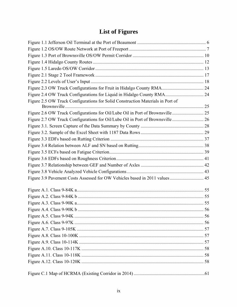
List of Figures

Figure 1.1 Jefferson Oil Terminal at the Port of Beaumont ........................................................... 6 Figure 1.2 OS/OW Route Network at Port of Freeport .................................................................. 7 Figure 1.3 Port of Brownsville OS/OW Permit Corridor ............................................................. 10 Figure 1.4 Hidalgo County Routes ............................................................................................... 12 Figure 1.5 Laredo OS/OW Corridor ............................................................................................. 13 Figure 2.1 Stage 2 Tool Framework ............................................................................................. 17 Figure 2.2 Levels of User’s Input ................................................................................................. 18 Figure 2.3 OW Truck Configurations for Fruit in Hidalgo County RMA.................................... 24 Figure 2.4 OW Truck Configurations for Liquid in Hidalgo County RMA ................................. 24 Figure 2.5 OW Truck Configurations for Solid Construction Materials in Port of

Brownsville ....................................................................................................................... 25 Figure 2.6 OW Truck Configurations for Oil/Lube Oil in Port of Brownsville ........................... 25 Figure 2.7 OW Truck Configurations for Oil/Lube Oil in Port of Brownsville ........................... 26 Figure 3.1. Screen Capture of the Data Summary by County ...................................................... 28 Figure 3.2. Sample of the Excel Sheet with 1187 Data Rows ...................................................... 29 Figure 3.3 EDFs based on Rutting Criterion ................................................................................ 37 Figure 3.4 Relation between ALF and SN based on Rutting ........................................................ 38 Figure 3.5 ECFs based on Fatigue Criterion ................................................................................. 39 Figure 3.6 EDFs based on Roughness Criterion ........................................................................... 41 Figure 3.7 Relationship between GEF and Number of Axles ...................................................... 42 Figure 3.8 Vehicle Analyzed Vehicle Configurations .................................................................. 43 Figure 3.9 Pavement Costs Assessed for OW Vehicles based in 2011 values ............................. 45

Figure A.1. Class 9-84K a............................................................................................................. 55 Figure A.2. Class 9-84K b ............................................................................................................ 55 Figure A.3. Class 9-90K a............................................................................................................. 55 Figure A.4. Class 9-90K b ............................................................................................................ 56 Figure A.5. Class 9-94K ............................................................................................................... 56 Figure A.6. Class 9-97K ............................................................................................................... 56 Figure A.7. Class 9-105K ............................................................................................................. 57 Figure A.8. Class 10-100K ........................................................................................................... 57 Figure A.9. Class 10-114K ........................................................................................................... 57 Figure A.10. Class 10-117K ......................................................................................................... 58 Figure A.11. Class 10-118K ......................................................................................................... 58 Figure A.12. Class 10-120K ......................................................................................................... 58

Figure C.1 Map of HCRMA (Existing Corridor in 2014) .............................................................61

x

Figure C.2 Map of Laredo (Existing Corridor 2014) .....................................................................66

Figure C.3 Map of Port of Brownsville (Existing Corridor 2014) ................................................67

Figure C.4 Map of Port of Freeport (Existing Corridor 2014) ......................................................71

Figure C.5 Map of Port of Corpus Christi (Existing Corridor 2014) ............................................74

xi

List of Tables

Table 2.1: Input for Corridor Network Attributes ........................................................................ 19 Table 2.2: Commodity Types in Hidalgo County ......................................................................... 22 Table 2.3: Commodity Types in Port of Brownsville ................................................................... 22 Table 2.4: Truck Configurations in Hidalgo County .................................................................... 23 Table 2.5: Truck Configurations in Port of Brownsville .............................................................. 23 Table 3.1: Highway Classes Used in the Bridge Analysis............................................................ 27 Table 3.2: Bridge Asset Value Percentages for GVW Categories ................................................ 31 Table 3.3: RHiNo and BRINSAP On-System Highway Classifications ...................................... 33 Table 3.4: Simulated Axle Loads and Configurations .................................................................. 37 Table 3.5: Equivalent Consumption Factors for Analyzed Vehicles ............................................ 43 Table 3.6: Mean Costs of Safety Projects ..................................................................................... 46 Table 4.1: Input for Corridor Network Attributes ........................................................................ 48 Table 4.2: Estimation of Pavement Consumption ........................................................................ 50 Table 4.3: Estimation of Bridge Consumption ............................................................................. 50 Table 4.4: Estimation of Safety Consumption .............................................................................. 51 Table 4.5: Estimation of Total Permit Fee Estimation ................................................................. 51 Table 5.1: Common Truck Configurations of Class 9 OW Trucks .............................................. 52 Table 5.2: Common Truck Configurations of Class 10 OW Trucks ............................................ 52 Table 5.3: Estimated Permit Costs of Existing Corridors ............................................................. 53

xii

List of Acronyms

AASHTO Association of State Highway and Transportation Officials

ACP asphalt concrete pavement

ALF axle load factor

BRINSAP Bridge Inventory, Inspection, and Appraisal System

CRCP continuously reinforced concrete pavement

ECF equivalent consumption factor

ESAL equivalent single axle load

GEF group equivalency factor

GVW gross vehicle weight

IMO International Maritime Organization

JCP jointed concrete pavement

LDF Laredo Development Foundation

MOANSTR Moment Analysis of Structures

OS oversize

OS/OW oversize/overweight

OW overweight

PCE passenger car equivalent

RMA Regional Mobility Authority

SN structural number

TEU twenty-foot equivalent unit

TxDMV Texas Department of Motor Vehicles

VMT vehicle miles traveled

1

Executive Summary

During the first year of project 0-6820, the research team completed Tasks 1 through 6: conducting a literature review, agreeing with TxDOT subject matter experts and PMC members on a framework for Stage 1 of the analysis, setting up a prototype version of the Stage 1 tool, and finalizing and submitting the full operational version of the Stage 1 tool. The second year of project 0-6820 involved the completion of the final project tasks. The research team conducted interviews and site visits; refined the Stage 2 Detailed Analysis Framework; performed pavement/bridge consumption, safety, and traffic operations analyses; developed the Stage 2 Prototype Detailed Analysis Tool; performed case studies; and held a workshop with ports and regional mobility authorities (RMAs) to present analysis results. This section will include a brief summary of each task completed during the second year. Task 7: Conduct Interviews and Site Visits with Ports and RMAs to Collect Field Data

To collect truck information to provide inputs for the design and calibration of the consumption models the research team made field visits to the following ports:

• Port of Beaumont

• Port of Victoria

• Port of Freeport

• Port of Corpus Christi

• Port of Brownsville

• Border gateways at Brownsville and Cameron County

• Hidalgo County RMA

• TxDOT Districts at Pharr and Laredo

• Laredo Development Foundation.

Task 8: Refine the Stage 2 Detailed Analysis Framework and Begin Developing Tool Modules

The Stage 2 Detailed Analysis Tool incorporated additional functionality and library information to enhance the user’s ability to perform safety and financial impact analyses of existing or proposed new overweight (OW) truck corridors serving coastal ports or border ports of entry. In this task, the research team proposed a new framework for the Stage 2 tool that was developed in Task 9 and Task 10. Chapter 2 provides an analysis of a permit sample from the existing corridors in the Port of Brownsville and Hidalgo County RMA was presented. Task 9: Perform Pavement/Bridge Consumption, Safety, and Traffic Operations Analyses and Develop Cost Factors

The Stage 2 tool has three cost analysis modules. Bridge and pavement consumption analyses provide estimates of the marginal costs caused by OW trucks in these infrastructures. Safety cost

2

accounts for required improvements of the corridor to mitigate potential safety impacts due to OW trucks. Chapter 3 details the results of this task. Task 10: Develop the Stage 2 Prototype Detailed Analysis Tool

In this task, the research team developed the Stage 2 prototype detailed analysis tool. In this tool, there are two “archived” corridors—the Port of Brownsville and Hidalgo County RMA oversize/OW corridors—with two truck configurations. The final Stage 2 tool has 12 different truck configurations and space for up to 13 more truck configurations if required in the future (25 in total). These additional truck configurations were implemented in in the tool. See Chapter 4 for more details. Task 11: Select Candidate Case Studies and Conduct Analyses

The research team selected candidate corridors for the case studies in this task—the existing corridors in Hidalgo County, Laredo, Port of Brownsville, Port of Freeport, and Port of Corpus Christi. The corridors analyzed are those existing in 2014. Chapter 5 presents the truck configurations included in Stage 2 tool, and the analysis results. Task 12: Conduct Workshop with Ports and RMAs to Present Analysis Results and Obtain Feedback

The research team hosted a workshop with representatives from ports, RMAs, and the trucking industry.

3

Chapter 1. Interviews and Site Visits with Ports and RMAs

1.1 Summary

1. The project scope was broadened to include both marine ports (deep water and shallow draft) and Texas/Mexico land gateways handling NAFTA freight.

2. Field visits were made to Texas ports at Beaumont, Victoria, Freeport, Corpus Christi, and Brownsville, and border gateways at Brownsville and Cameron County, Hidalgo County Regional Mobility Authority (RMA), the TxDOT Districts at Pharr and Laredo, and the Laredo Development Foundation.

3. The visits confirm that a number of county oversize/overweight (OS/OW) networks are being managed, constructed, developed, or promoted actively in Texas. The length, funding, maintenance, design, and pricing vary substantially between ports and border gateways but both types of entities are driven by remaining competitive with other Texas entry points, particularly those dealing with NAFTA and international trade.

4. Marine ports identify handling OW containers1 (especially export) and loads (especially import) that can be more efficiently moved by Mexican trucks. Current interest centers on managing single-trip toll road permits to recover infrastructure consumption, rather than multi-trip permits like those referenced in HB 2016.

5. OS/OW routes are already permitted in Cameron, Hidalgo, Webb, and Maverick counties and link Texas/Mexico ports of entry with transload facilities in nearby counties. All differ in network, purpose, cost to operate, permit prices, and customer demand.

6. All county staff contacted during the visits agreed to evaluate the tools developed in the project. The wide disparity in current ton/mile toll prices shows that prices are determined by estimation rather than analysis.

1.2 Background

Texas follows the federal limits on truck size and weight dimensions unless the truck load is operating under an approved legislative permit. The state allows a wide variety of annual permits (as noted in Box 1) related principally to agricultural or raw material production, and offers trucking companies a single-trip permit issued by the Texas Department of Motor Vehicles (TxDMV). The TxDMV permit process uses a computer program—

1 The International Maritime Organization intends to introduce a container weight rule change on July 1, 2016, that will require shippers to weigh loaded containers before they are loaded at the port of origin.

Box 1: Rider 36 Study

Increased OS/OW truck traffic in Texas associated with a growing population and economy has amplified long-standing concerns about the impact of that traffic on Texas highways. In many instances, OS/OW trucks are operating over highways, roads, and bridges not designed for either the weight or volume of that traffic. In fiscal year (FY) 2011, the state issued almost 600,000 permits for loads that exceeded state and federal size and weight limitations and generated $111 million in revenue.

Source: TxDOT Rider 36 OS/OW Vehicle Fees Study

4

Texas Permitting and Routing Optimization System or TxPROS—to route the load based on gross weight, axle weight distribution, height, width, and suitable Texas highways from origin to destination. These loads are often accompanied by escort vehicles to inform other road users and improve trip safety.

Heavy indivisible loads that enter Texas through both maritime ports and border gateways move under TxDMV single-trip permits and their routes may take up to 3 years in the planning if they’ll need bridge infrastructure that requires strengthening. However, an increasing number of county networks catering to vehicles in the 90,000 to 125,000 pound gross vehicle weight (GVW) category2 have emerged in the last 4 years and more are predicted to emerge as interim bills in the 2017 Texas Legislative session. In addition, the International Maritime Organization3 (IMO), responding to the container line membership on the World Shipping Council (which controls 90 percent of global container capacity), has pushed for the implementation by July 1, 2016, of a rule to weigh all loaded containers at the port of origin. The shipper, under this rule change, will physically weigh the loaded container and provide carriers with a signed Verified Gross Mass document before it is loaded for export.

This action was promoted by the IMO Safety of Life at Sea (SOLAS) Convention based on concerns from steamship companies that an unknown number of heavy containers could cause ship instability and even loss in bad weather. A secondary issue is that OW containers create a series of problems at destination ports. OW containers arriving at the Port of Houston require a single-trip permit, special treatment, or transloading, which lowers terminal efficiency. The issue of OW export containers has important strategic impacts at some Texas deep water ports over the past 2 years. This issue arises because many of the port destinations for Texas exports—plastic pellets, for example—are in countries where higher truck weights are permitted4. The Port of Freeport has already obtained legislative support for a small toll road system linking several Dow chemical plants in its immediate hinterland to move 97,000 lb. GVW vehicles, which suggests a container weight of over 60,000 lb.5 Maritime ports and border gateways are competitive and all want an equal footing when pricing for services so it is not unexpected that ports and gateways are exploring their options to have OS/OW links serving their terminals, transload centers, brokers, or key customers. However, it became clear that the prices set for these smaller toll road systems appeared arbitrary and not based on consumption factors for pavements and bridges.

The Texas Legislature has established four OS/OW corridors to serve the Ports of Corpus Christi, Brownsville, Freeport, and Victoria6. Once a corridor’s legislation is enacted by the Legislature and signed by the Governor, the Texas Transportation Commission prepares a written agreement with the sponsoring local agency. It is based upon prior discussions between TxDOT and the local agency to determine the location of the corridor, the permit fee amount, and any operating conditions. Under these agreements, the local agency issues the OS/OW permits to users and collects fees to cover the maintenance cost of the corridor. Importantly, the local agency (i.e., the

2 This reflects the failure of an original NAFTA provision to standardize truck size and weight limits between the three countries within 10 years of signing the agreement. Canada and Mexico allow trucks in this weight range to operate on key corridors of their highway systems. 3 The IMO is a specialized agency of the United Nations with 171 Member States. 4 All EU counties have 40 metric ton (97,000 lb.) GVW limits. 5 The EU requires such weights to be carried on six axles using a tridem semitrailer chassis. 6 These corridors can be found in Chapter 623 of the Texas Transportation Code.

5

port) takes full responsibility for the corridor’s maintenance. If the OS/OW permit fees are inadequate to cover the additional maintenance costs, the port must make up the difference.

This TxDOT research project, involving researcher teams at the Center for Transportation Research and UT-San Antonio, was designed to remedy this inadequacy. It has two products designed to assist TxDOT staff, RMA staff, port and border gateway staff, and city planners develop effective costs. The first product uses general cost factors to provide efficient answers to questions regarding pavement and bridge consumption rates. The second product provides a more detailed analysis method of Texas pavement and bridge consumption costs based on historical permit sales and the anticipated types of trucks, truck configurations, and loads.

These tools provide TxDOT with the means to answer questions and discuss specific cost analysis processes with local authorities planning to propose a new corridor or already managing an existing corridor. In addition, the tools will provide TxDOT with methods based on sound engineering practice and prior consideration of the factors related to OS/OW truck corridor operations when responding to questions from the State Legislature, TxDOT Transportation Commission, and TxDOT Administration.

Truck size and weight limits vary substantially between the three NAFTA signatories and Texas allows over 20 different types of permit that exceed U.S. Federal Interstate limits. It is critical that any engineering model used to estimate consumption rates reflects, with some degree of accuracy, the price levied by the toll authority on each truck. Ideally, each truck would be allocated a unique consumption rate per mile and charged for the mileage traveled on the system. And since trucks are often unloaded in one direction, the price of the toll should vary to reflect this impact. Box 2 describes an economically equitable truck toll pricing system that would achieve this objective. Unfortunately, although mechanisms exist to capture both elements of the toll, they are rarely used and crude estimates are typically made to average out the wide range of consumption rates.

The use of rough estimates is unfortunate because trucking is highly competitive and companies standardize on the most efficient truck model within each class. Thus, that approach effectively reduces the variety of trucks using the toll facility. For example, 70 percent of interstate trucks are five-axle articulated vehicles running 53-ft. semi-trailers. This suggests that users operating regularly over toll roads, wherever the roads were located, choose similar truck types and designs7 to compete for the cargo.

A series of field visits were scheduled in this project to collect this type of truck information to provide inputs for the design

7 There will always be differences in engine performance and transmissions depending on the average speed of the overall trip.

Box 2: An Idealized Equitable Toll System

The truck would enter the OS/OW network and pass over a weigh-in-motion (WIM) system that would measure axle and gross weights, axle spacing and calculate the truck equivalent axle load, which drives pavement consumption. The axle and gross loads would link to a structural (bridge) consumption sub-model. The remaining input is vehicle miles of travel loaded and unloaded. The first entry onto the toll system identifies the truck; as it returns, any change in gross weight is noted and the toll rate per mile adjusted. This method addresses the joint issues of equity and efficiency.

6

and calibration of the consumption models. The field visits included marine ports at Beaumont, Victoria, Freeport, Corpus Christi, and Brownsville, and border gateways at Brownsville and Cameron County, Hidalgo RMA, the TxDOT Districts at Pharr and Laredo, and the Laredo Development Foundation. Appendix B provides an example of the questions used, with modifications where necessary, at the field visit.

1.3 Field Visits: Marine Ports

1.3.1 Port of Beaumont

John Roby at the Port of Beaumont provided a port tour in September 2015 and answered the questionnaire. Currently, there are no immediate plans to promote and/or operate an OS/OW system linking the port8. TxDMV permits are used for any OS/OW single-trip permits, which appear to adequate for the type of cargo currently moving through the port. Investment at the port has focused on two areas: first, improving the handling—loading and unloading—of military cargo associated with its position as a key gateway for military deployment, especially heavy equipment moved by train from Fort Hood; second, devloping a $300 million multi-modal oil receiving area named Jefferson Terminal (see Figure 1.1).

Figure 1.1 Jefferson Oil Terminal at the Port of Beaumont

Unit trains of heavy crude arrive from Colorado and the Bakken oil field of North Dakota and are stored in tanks, prior to being mixed with lighter crude; this mixture is then sent to Texas refineries

8 A petro-chemical company located close to the port did examine an OS/OW route for moving heavy containers of plastic pellets for export but concluded that the lack of a regular container on barge service made it impractical.

7

for chemical, petro-chemical, and fuel production. In addition, local state oil from fracking, which is not served by pipelines, arrives on site so that it serves three modes—rail, barge9, and truck.

1.3.2 Port of Freeport

The Port of Freeport, contacted in November 2015, provided information on their toll network located in the immediate hinterland. The port sought and obtained legislative action to permit trucks up to 97,000 lbs. on the network. The port is located on a 45-ft. channel currently under review for expansion to 55 ft. on the Texas coast. It currently handles over 100,000 TEU (twenty-foot equivalent unit) annually and specializes in fruit imports (bananas) for the Dole Company, carried on Maersk containerships. The port has excellent rail service that is sometimes used by shippers importing wind equipment such as blades and tower parts. Its exports include chemicals, paper goods, and resins; this aspect of its business drives the interest in the OS/OW toll road system. See Figure 1.2.

Figure 1.2 OS/OW Route Network at Port of Freeport

The main commodity to be handled by the OS/OW system, in the immediate future, was to allow chemical plants to move containerized export products—especially plastic pellets—in heavier quantities that comply with higher size and weight limits in the country into which the products are imported. This would certainly make exports less expensive in U.S. dollar terms, which is currently a critical constraint in global trade.

9 Barges move final products from Jefferson using the Gulf Intracoastal Waterway to serve Texas coastal refineries.

8

1.3.3 Port of Corpus Christi

The Port of Corpus Christi was contacted in September 2015 and a field visit was made to interview the Port Executive Director, John LaRue. The port has always played a critical role in the Texas economy and is the eighth largest U.S. port in terms of total tonnage. Oil imports have traditionally been the largest sector in the port’s business due to the proximity of three large petro-chemical plants. However, over the last 4 years, oil imports have been overtaken by oil exports, first from the Eagle Ford shale play. Pipelines have gained a strong market share of shale oil plays and in 2016 the port will be connected to the Permian Basin field via a 40-inch diameter pipeline. The Port has two OS/OW highways, one on the Joe Fulton International Trade Corridor, which links to IH 37, and a second that uses a 2-mile section of the city network to reach a different point on the same interstate highway. The city permit is based on gross weight and axle distribution and whether a police escort is needed. Then the toll fee is calculated and issued. The Port does not have a container liner service and the needs of shippers dealing with OS/OW cargo center on breakbulk and wind components10. Mr. LaRue said that a large consignment of blades and related tower equipment was booked for arrival in the early part of 2016. This cargo is almost always moved by single TxDMV permits and is not suitable for sustaining a toll road system, however small. In addition, project cargo also moves from the port by rail and it is estimated that about half of the projected wind cargo during the 2016–17 period will be shared by both modes.

1.3.4 Port of Brownsville

The Port of Brownsville has benefitted from operating an OS/OW toll road since 1998 and it still plays an important role as a port of entry for Mexican manufacturing. Mexican trucks can purchase an OS/OW permit to carry cargoes from the Port of Brownsville to the Gateway International Bridge (via SH 48/SH 4) and the Veterans International Bridge at Los Tomates (via US 77/US 83 and SH 48/SH 4). These permits allow gross weight to reach the legal weight limit for Mexican 6-axle trucks11, which is 125,000 pounds. Dimensionally, the combined vehicle and load cannot exceed 12 feet in width, 15.5 feet in height, and 110 feet in length. The ability to access an OS/OW toll road reduces transloading steps in the supply chain by one—which translates into lower trucking costs and makes the port more competitive in global trade. All agencies undertaking toll highways have visited the port to gain experience from arguably the most successful operator of a regional county toll system.

Box 3 summarizes the main features of the Brownsville system. The first year it opened, around 28,000 permits were issued, priced at $30 for a single-trip fee.

10 The Port of Corpus Christi also handles military deployment and supports the primary role of the Port of Beaumont when needed. 11 These configurations include a triple (tridem) axle semi-trailer, the typical truck serving the Port of Brownsville.

9

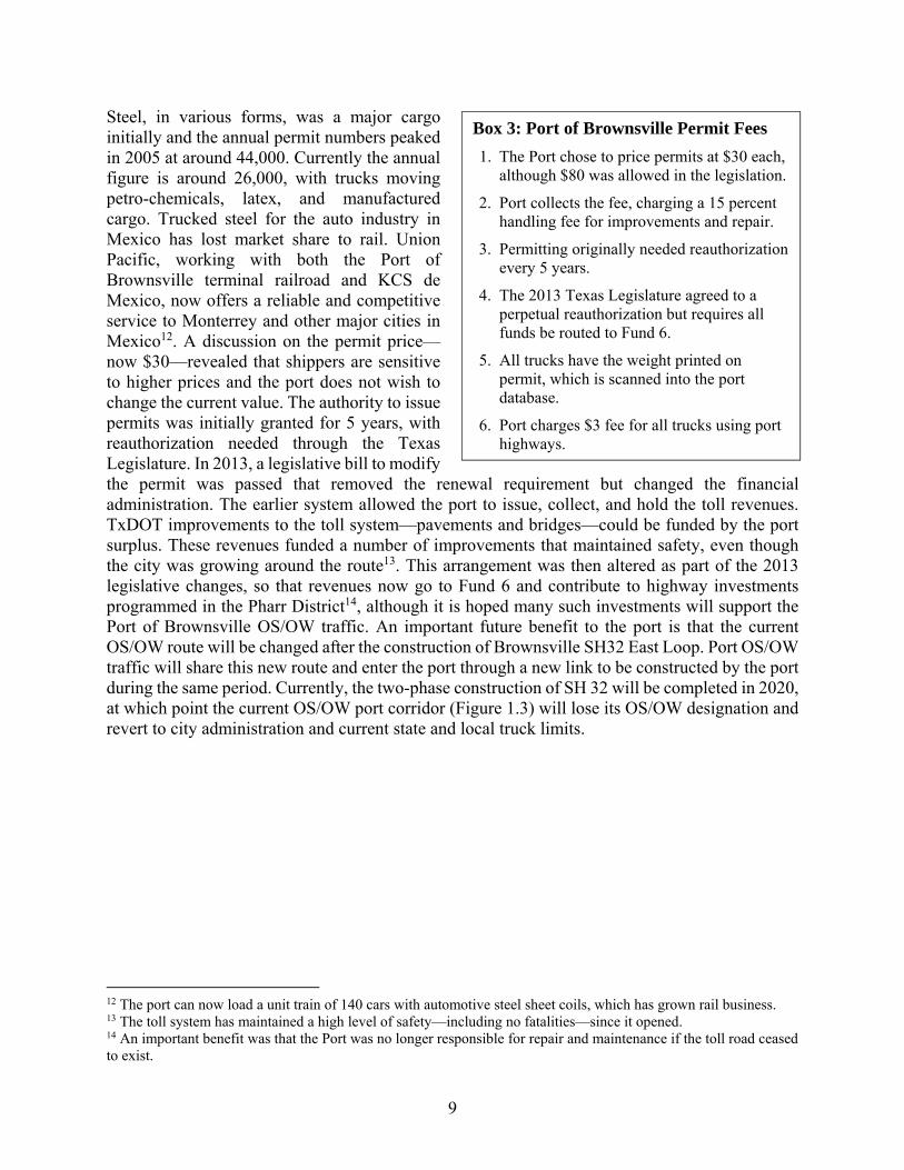
Steel, in various forms, was a major cargo initially and the annual permit numbers peaked in 2005 at around 44,000. Currently the annual figure is around 26,000, with trucks moving petro-chemicals, latex, and manufactured cargo. Trucked steel for the auto industry in Mexico has lost market share to rail. Union Pacific, working with both the Port of Brownsville terminal railroad and KCS de Mexico, now offers a reliable and competitive service to Monterrey and other major cities in Mexico12. A discussion on the permit price—now $30—revealed that shippers are sensitive to higher prices and the port does not wish to change the current value. The authority to issue permits was initially granted for 5 years, with reauthorization needed through the Texas Legislature. In 2013, a legislative bill to modify the permit was passed that removed the renewal requirement but changed the financial administration. The earlier system allowed the port to issue, collect, and hold the toll revenues. TxDOT improvements to the toll system—pavements and bridges—could be funded by the port surplus. These revenues funded a number of improvements that maintained safety, even though the city was growing around the route13. This arrangement was then altered as part of the 2013 legislative changes, so that revenues now go to Fund 6 and contribute to highway investments programmed in the Pharr District14, although it is hoped many such investments will support the Port of Brownsville OS/OW traffic. An important future benefit to the port is that the current OS/OW route will be changed after the construction of Brownsville SH32 East Loop. Port OS/OW traffic will share this new route and enter the port through a new link to be constructed by the port during the same period. Currently, the two-phase construction of SH 32 will be completed in 2020, at which point the current OS/OW port corridor (Figure 1.3) will lose its OS/OW designation and revert to city administration and current state and local truck limits.

12 The port can now load a unit train of 140 cars with automotive steel sheet coils, which has grown rail business. 13 The toll system has maintained a high level of safety—including no fatalities—since it opened. 14 An important benefit was that the Port was no longer responsible for repair and maintenance if the toll road ceased to exist.

Box 3: Port of Brownsville Permit Fees

1. The Port chose to price permits at $30 each, although $80 was allowed in the legislation.

2. Port collects the fee, charging a 15 percent handling fee for improvements and repair.

3. Permitting originally needed reauthorization every 5 years.

4. The 2013 Texas Legislature agreed to a perpetual reauthorization but requires all funds be routed to Fund 6.

5. All trucks have the weight printed on permit, which is scanned into the port database.

6. Port charges $3 fee for all trucks using port highways.

10

Figure 1.3 Port of Brownsville OS/OW Permit Corridor

The research team asked port officials whether the toll road networks in Cameron and Hidalgo counties would be connected in the future to offer a multi-county network. It was acknowledged that there were obvious regional economic and political benefits from merging—such a merger would produce the third largest MPO 15 in Texas. Additionally, a regional approach would strengthen gateways in the Valley with Brownsville, the nearest deep water port. The Class 2 railroad system16 running through the Valley to Brownsville would also provide an alternative mode. However, it was thought that it would take time to balance the financial benefits with administrative costs of power sharing and county staff rationalization.

1.3.5 Hidalgo County Field Visits

Three visits were made to agencies in Hidalgo county: McAllen Economic Development Council (Executive Director Keith Patridge), Hidalgo County RMA (HCRMA Executive Director Pilar Rodriguez), and the TxDOT Pharr District office (TPP Director Homer Bazan and Advanced Planning/RMA Coordinator Norma Garza).

15 This would elevate the two counties to megaregion status; if Webb County joined, it would form a national megaregion in terms of population and economic activity. 16 The line was originally part of the Union Pacific system so integration would not be technically difficult.

11

The McAllen Foreign Trade Zone #12 was created in 197317, making it the first non-marine inland U.S. trade zone. It subsequently played an important role in developing the Valley, most especially the development of the Reynosa maquiladora plants, which employ over 12,000 workers. Mr. Patridge was engaged throughout the process, which ultimately produced the Hidalgo RMA OW network, and believes the central corridor in the network will carry a majority of traffic over the initial years of operation. He supported the project because it offered a more efficient process of transporting produce to county transloading plant locations where value is added. Pharr is the #2 importation gateway for Mexican produce, and offering an OW route within the county (thus allowing legally loaded Mexican trucks to go directly to the transloading plants) provided an estimated cost saving of $600 to $1200 per trip. He made no reference to permit numbers or cost but did say that a number of county locations were incorporated into the final RMA network. He believed that most produce trucks would be less than 100,000 lb. GVW carried on five-axle semi-trailer trucks, which complies with the produce permit weights but not the juice carried in tanker trucks. He closed by saying that the OW corridor should play a role in the exploration of gas and oil in northern Mexican plays but agreed that current prices did not justify further exploration until the market adjusted upwards.

The second visit was to the offices of the Hidalgo RMA, where Executive Director Pilar Rodriguez was interviewed. He stated that an estimated 12,000 permits would be issued in the first year of operation. The OW corridor is currently using existing highways in the county, so there should be a mix of predominantly U.S. legally loaded trucks, interspersed with heavier Mexican trucks running under RMA permit. He stated that a 2014 TTI study18 found that many of the U.S. trucks were overloaded. During a period when 300 permits were issued, over a thousand trucks were measured as exceeding Texas gross loads, which raised the challenge of enforcement. The permit allows Mexican trucks to operate up to 125,000 lb. GVW but Mr. Rodriguez agreed that no produce trucks would need that limit. The permit is for a single trip and is not graduated based on consumption rates. The RMA is about to issue a request for bids for a major portion of the toll road—SH 365—and it is estimated that construction will take 30 months to place into service. Figure 1.4 maps area routes.

17 See mcallenftz.org. 18 US 281–Pharr: Traffic Load Spectra Analysis with the Portable TRS WIM, TxDOT IAC Project # 0-409162, November 2014

12

Figure 1.4 Hidalgo County Routes

There are no plans to link with the Cameron County OS/OW system. Instead, the RMA strategy is to develop SH 365 as the core of the system, meeting east-west traffic while north-south spurs will be updated as necessary but not replaced. On the matter of data for planning and research activities, the RMA is currently not identifying the links selected by the truckers, just the destination of the loads.19 It is clear that the Hidalgo System is the most ambitious of any currently planned along the Texas-Mexico border and will go through several changes before it is operating efficiently. The RMA would like to test the beta version of this project’s first product when it is available, as Mr. Rodriquez believes that the current $80 permit fee is insufficient to cover the actual pavement and bridge consumption.

The third meeting was held at the Pharr District office of TxDOT where Homer Bazan and Norma Garza provided background planning and programming material on both Hidalgo and Cameron County OS/OW systems. They confirmed that OW traffic will use current state highway segments until SH 365 is let for construction. The east segment is scheduled for bidding in late 2017 and the west segment one year later, with the complete highway estimated to open in mid-2020. They wished to be kept advised on research progress and would like to examine the beta product when it is available. Ms. Garza was designated as the contact person since she is the RMA Coordinator.

1.3.6 Laredo District

Three visits were made to Laredo: first to meet TxDOT District Engineer Pedro Alvarez and District Administrator Melissa Montemayor, then to interview staff at the Laredo Development

19 This is not a critical issue because truckers can be assumed to take the shortest and safest route to the consignee address. Weight data is apparently entered into the permit database but is not on the ticket.

13

Foundation (LDF), and finally to meet with Carlos Casellas at Con-way Truckload,20 which handles large cargos for Caterpillar, including non-divisible OS/OW components.

The visit to the District Office confirmed that they are examining the various elements of an OW corridor passed during the 2015 Legislative session. The route, shown in Figure 1.5, has some unusual characteristics.

Figure 1.5 Laredo OS/OW Corridor

First, the route enters Laredo at the World Trade Bridge—the most congested northbound bridge on the entire U.S-Mexico border. This is odd, since Con-way moves OS loads through Colombia or via other Texas-Mexico bridges because of higher service levels. It links to FM 1472—the Mines Road—which has the highest concentration of trucks on any Texas FM highway. This segment is notorious during the peak afternoon hours when level of service drops substantially. The route then moves sharply north east and uses highway segments that either need building or reconstructing. Most critically, this fails to service most of the brokers or transload centers located

20 Con-way and Menlo Logistics are now merged under XPO Logistics.

14

within city boundaries. Next, the fee is set at $200, which is unlikely to generate many customers21 unless it is the upper boundary of the fee structure. Finally, the legislation appears to have been undertaken without receiving input from the members of the LDF. I paid a second visit to the LDF and presented details of this project to an audience that included the mayor of Laredo. I understand that subsequently, it was agreed that the whole city should be considered open to permitted OS/OW vehicles, although that creates a whole new series of planning, construction, and funding issues.

1.4 Conclusions

1. The field visits opened a dialog with a variety of beneficiaries and agencies with a financial interest in allowing Mexican trucks to travel under OS/OW permits to border transload centers. Frankly, the opportunity lies with OW trucks since OS and large indivisible loads generally travel under a single-trip TxDMV permit. Weight, rather than dimensions, is the key interest at all the ports visited, whether they are marine or border gateways. At every visit, those interviewed expressed willingness to test the beta versions of the study products when they become available.

2. All port and border OW fees have can be adjusted to a maximum of $200 per trip, although there is a disparity in actual permit fees, ranging from $30 to $200. The fees appear to be estimated on what the market will bear, rather than the actual consumption each truck imposes on the toll system.

3. In economic terms, marginal prices should not be the rule for Mexican trucks since they pay no Texas registration fees. This means the consumption rates should be measured in terms of total ESAL (equivalent single axle load) costs and not marginal costs.

4. Equally important, permit fees should reflect the trip length where networks are used. Point-to-point routes, like that of the Port of Beaumont, have a fixed length, which simplifies the estimation of the toll.

5. It is suggested that the first product of this project (a) calculate the marginal per-mile cost of a 97,000 lb. tridem trailer container truck for a Texas marine port, (b) the total per-mile consumption cost for a five-axle Mexican truck at 95,000 lb., and (c) the total per-mile consumption cost of a six-axle Mexican tridem semi-trailer truck at 120,000 lb.

21 A broker at the Laredo Development Foundation meeting stated that it was over half the total fee charged for moving loads from Monterrey to Laredo. It also runs counter to the arguments made in Brownsville based on the survey of their customers.

15

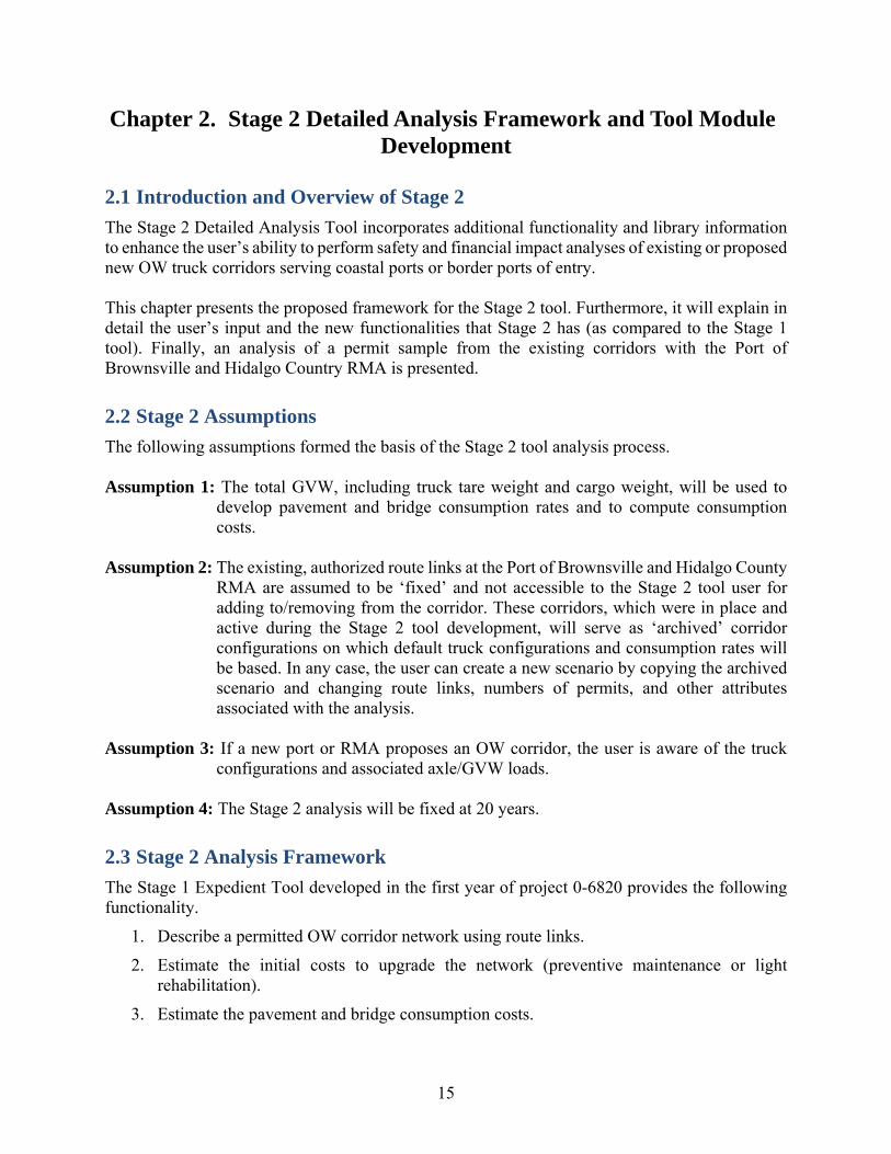
Chapter 2. Stage 2 Detailed Analysis Framework and Tool Module Development

2.1 Introduction and Overview of Stage 2

The Stage 2 Detailed Analysis Tool incorporates additional functionality and library information to enhance the user’s ability to perform safety and financial impact analyses of existing or proposed new OW truck corridors serving coastal ports or border ports of entry. This chapter presents the proposed framework for the Stage 2 tool. Furthermore, it will explain in detail the user’s input and the new functionalities that Stage 2 has (as compared to the Stage 1 tool). Finally, an analysis of a permit sample from the existing corridors with the Port of Brownsville and Hidalgo Country RMA is presented.

2.2 Stage 2 Assumptions

The following assumptions formed the basis of the Stage 2 tool analysis process. Assumption 1: The total GVW, including truck tare weight and cargo weight, will be used to

develop pavement and bridge consumption rates and to compute consumption costs.

Assumption 2: The existing, authorized route links at the Port of Brownsville and Hidalgo County

RMA are assumed to be ‘fixed’ and not accessible to the Stage 2 tool user for adding to/removing from the corridor. These corridors, which were in place and active during the Stage 2 tool development, will serve as ‘archived’ corridor configurations on which default truck configurations and consumption rates will be based. In any case, the user can create a new scenario by copying the archived scenario and changing route links, numbers of permits, and other attributes associated with the analysis.

Assumption 3: If a new port or RMA proposes an OW corridor, the user is aware of the truck

configurations and associated axle/GVW loads. Assumption 4: The Stage 2 analysis will be fixed at 20 years.

2.3 Stage 2 Analysis Framework

The Stage 1 Expedient Tool developed in the first year of project 0-6820 provides the following functionality.

1. Describe a permitted OW corridor network using route links.

2. Estimate the initial costs to upgrade the network (preventive maintenance or light rehabilitation).

3. Estimate the pavement and bridge consumption costs.

16

4. Calculate estimated total corridor costs and a permit fee.

5. Determine the financial impact of the corridor.

6. Prepare a report documenting inputs, outputs, assumptions, and results. The Stage 2 Detailed Analysis Tool will have the following additional functionality.

1. Estimate, using refined values, the pavement and bridge consumption cost.

2. Estimate two different permit structures:

a. Universal permit for all trucks

b. Specific permit for different truck configurations

2.3.1 Stage 2 Analysis Tool Framework

The Stage 2 Analysis Tool framework is composed of five elements: User Input Modules, Data Library, Project Information, Cost Analysis, and Recommendations on Permit fee/Reports, as shown in Figure 2.1.

17

Figure 2.1 Stage 2 Tool Framework

In the first part, the user needs to introduce required information about the corridor that will allow the Stage 2 tool to estimate a permit fee. This information will be stored as project information in the Stage 2 tool. In the next phase of Stage 2, the tool will link the attributes of the network with the information store from the analysis. There are three sources of consumption cost: pavement, bridge, and safety projects (optional). The user will be able to make the decision of whether to implement a specific safety project. Finally, the Stage 2 tool estimates the consumption cost of OW trucks in the network. Likewise, it will estimate the permit fee, and present the allocation to related agencies based on the permit structure.

18

User Input Modules

User input modules consist of three levels: Corridor Network Level, Route Level, and Segment Level, as in Figure 2.2.

Figure 2.2 Levels of User’s Input

In Corridor Network Level, the user’s input consists of basic corridor information (e.g., corridor name), OW traffic information (e.g., the number of trucks in the first year of operation), and permit information (if there is information available). The specific information needed is summarized in Table 2.1.

Segment LevelRoute LevelCorridor Network LevelCorridor network attributes

Route 1 attributesSegment 1 attributesSegment 2 attributes

…Route 2 attributes…

19

Table 2.1: Input for Corridor Network Attributes Corridor Network Level Inputs

General Corridor Information

OW Traffic Information Permit Information

Corridor Name Estimated OW Trucks in the

First Year of Analysis Current Permit Fee

Corridor Comments Annual Growth Rate Deduction Agency 1

Percentage of Trucks Following Configuration 1

Percentage of the Fee for Agency 1

Percentage of Trucks Following Configuration 2

Deduction Agency 2

… Percentage of the Fee for

Agency 2

… In Route Level, the user will need to input the characteristics of the road. Following are the attributes at this level:

1. Route functional class posted.

2. Route number (for example, if it is State Highway 48, it should be "48").

3. Route comments (anything the user wants to store about the route; for example: “This is a new corridor”).

Because the pavement consumption cost and the bridge consumption cost depend on different factors (for example, various pavement type), it is required to segment the routes in the network to estimate properly the consumption. For example, the same route could present both asphalt concrete pavement and jointed concrete pavement segments. In this case, both types of pavement need to be separated in segments, in order to estimate properly the consumption cost. Therefore, the next level (Segment Level) is used for pavement consumption and bridge consumption analysis. The segments in a route are defined by four criteria:

1. If there is change in pavement materials, the route should be divided into different segments. Pavement type will impact the pavement consumption analysis.

2. If route crosses both rural and urban areas, it should be divided into different segments. The bridge consumption rate is different in rural and urban areas.

3. If there is an intersection on the route, the route should be divided into different segments by intersection. The presence of an intersection will change the composition of the truck traffic, which leads to different consumption results.

4. If route goes across different counties, it should be divided into different segments by county line. The bridge consumption rate varies from county to county.

20

Based on the route segmentation criteria, the following information will be needed for each segment: number of lanes, roadbed information, length (miles), pavement type, percentage of OW trucks in the segment, county where the segment is located, bridge location (urban/rural), total safety cost, and other comments on the segment.

Data Library, Project Information, and Cost Analysis

The Data Library consists of the following data types:

• Corridor networks

• Routes in the corridor network

• Truck configurations analyzed

• Cost-related parameters

o Pavement consumption cost

o Bridge consumption cost

o Road safety projects cost The Data Library is for existing corridors or corridors saved by the user previously. If the user wants to analyze a new corridor, the user would need to know the distribution of truck configurations (i.e., what percentage of each OW truck configuration will use the network). It is important to mention that the Stage 2 tool will include a component of cost associated with road safety projects. The tool will include a list of potential projects (for example, widen the road 3 ft, install traffic lights, install flashing beacons, etc.) with their associated cost as references. However, the user will need to input the proper value for each of these improvements. By compiling the user input, the Data Library, and the corridor upgrade decisions, the project information will be available for the cost analysis. The truck consumption for pavements, bridges, and safety upgrades can be calculated based on the truck configurations and segment characteristics. The total OW corridor network consumption cost is then estimated as the sum of all the pavement, bridge, and safety costs.

Recommendations on Permit Fee/Reports

Based on the total OW corridor network consumption cost, the tool can estimate the fiscal impact and the permit fee for TxDOT to reach a break-even point.

2.4 New Modules in the Stage 2 Tool

The Stage 2 tool will provide a new module, which will generate different permit fee structures. This new module will give the user the option to either generate a universal permit fee for all the trucks or generate different recommended permit fees for trucks in different configurations. It will encourage infrastructure-friendly axle configurations (thus reducing pavement and bridge consumption).

21

Two additional modules were considered for inclusion in the Stage 2 tool but ultimately not included: a module for incorporating the Structural Condition Index (SCI) method and a module for estimating OW truck traffic. The objective of the SCI module was to assess the need for pavement treatments. However, because of the complexity of pavement data, and the need to update it continually, the Research Team felt that this analysis should be kept separated from the consumption cost analysis. The second module (for estimating OW truck traffic) was designed to use information from the existing corridors to predict OW traffic and thus predict the number of permits needed in new corridors. However, lack of data prevented the module’s incorporation—currently, truck traffic data is available for only two corridors, which is insufficient for accurate predictions for new corridors. The Research Team did analyze the information available, however; the next section presents the results of this analysis.

2.5 Analysis of Existing Corridors

The sample of permit data was analyzed in order to obtain a deep understanding of the existing situation on those corridor networks. Permit data from Hidalgo County and Port of Brownsville was analyzed separately with the same method. First, the research team analyzed the commodities that are transported in each corridor. The commodity types on trucks in Hidalgo County are categorized into the following five groups:

1. Produce-Fruit: banana, broccoli, orange, etc. 2. Metals: steel 3. Cotton 4. Produce-Liquid: juice, orange concentrate, etc. 5. Undefined: Mexico, USA, “Mixto”, etc.

The commodity types on trucks in Port of Brownsville fall into the following eight categories: 1. Produce-Fruit: vegetables, grains, etc. 2. Construction Materials (Solid): steel, paper, sand, etc. 3. Cotton 4. Oil Products 5. Undefined: “sacos”, “planchon”, etc. 6. Bottles & Drinks: vegetable oil, orange juices 7. Asphalt 8. Chemicals

Permit statistics for the commodity types in each corridor network are shown in Table 2.2 and Table 2.3.

22

Table 2.2: Commodity Types in Hidalgo County

No. Categories No. Of Permits

% Weight %

01 Produce-Fruit 911 62.4% 79,380,996 59.5%

02 Metals 1 0.1% 82,536 0.1%

03 Cotton 1 0.1% 80,070 0.1%

04 Produce-Liquid 191 13.1% 22,287,211 16.7%

05 Undefined 355 24.3% 31,662,058 23.7%

Table 2.3: Commodity Types in Port of Brownsville

No. Categories No. Of Permits

% Weight %

00 Other - 0.0% - 0.0%

01 Produce-Fruit 18 0.2% 1,430,057 0.2%

02 Construction Materials (Solid) 4,787 53.6% 465,641,696 54.7%

03 Cotton 30 0.3% 2,464,140 0.3%

04 Oil Products 2,526 28.3% 230,811,633 27.1%

05 Undefined 164 1.8% 14,709,361 1.7%

06 Bottles & Drinks 35 0.4% 3,426,610 0.4%

07 Asphalt 59 0.7% 5,768,420 0.7%

08 Chemicals 1,314 14.7% 127,625,579 15.0%

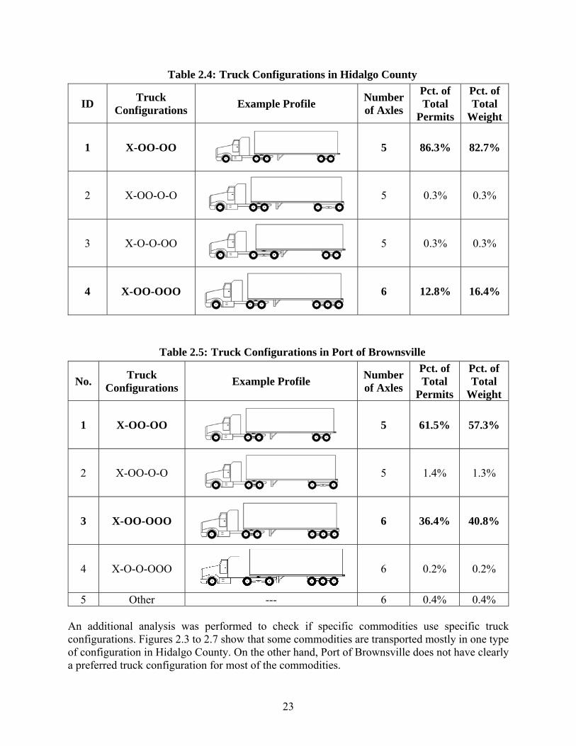
Then the truck configurations were also analyzed. To categorize a truck configuration, the following convention is used:

• Single Tire Axle: The single tire axles are represented by a “X”

• Dual Tire Axle: The dual tire axles are represented by an “O”

• Separated Axle: If there is a separation between axles that is greater than 8 feet, it is represented by a “-”.

The primary truck configurations in each county are provided in Table 2.4 and Table 2.5.

23

Table 2.4: Truck Configurations in Hidalgo County

ID Truck

Configurations Example Profile

Number of Axles

Pct. of Total

Permits

Pct. of Total

Weight

1 X-OO-OO

5 86.3% 82.7%

2 X-OO-O-O

5 0.3% 0.3%

3 X-O-O-OO

5 0.3% 0.3%

4 X-OO-OOO

6 12.8% 16.4%

Table 2.5: Truck Configurations in Port of Brownsville

No. Truck

Configurations Example Profile

Number of Axles

Pct. of Total

Permits

Pct. of Total

Weight

1 X-OO-OO

5 61.5% 57.3%

2 X-OO-O-O

5 1.4% 1.3%

3 X-OO-OOO

6 36.4% 40.8%

4 X-O-O-OOO

6 0.2% 0.2%

5 Other --- 6 0.4% 0.4% An additional analysis was performed to check if specific commodities use specific truck configurations. Figures 2.3 to 2.7 show that some commodities are transported mostly in one type of configuration in Hidalgo County. On the other hand, Port of Brownsville does not have clearly a preferred truck configuration for most of the commodities.

24

Figure 2.3 OW Truck Configurations for Fruit in Hidalgo County RMA

Figure 2.4 OW Truck Configurations for Liquid in Hidalgo County RMA

X-OO-OO99%

X-OO-OO X-OO-O-OX-O-O-OO X-OO-OOO

X-OO-OO3%

X-OO-OOO97%

X-OO-OO X-OO-O-OX-O-O-OO X-OO-OOO

25

Figure 2.5 OW Truck Configurations for Solid Construction Materials in Port of Brownsville

Figure 2.6 OW Truck Configurations for Oil/Lube Oil in Port of Brownsville

X-OO-OO52%

X-OO-O-O2%

X-OO-OOO45%

X-OO-OO X-OO-O-OX-OO-OOO X-O-O-OOO

X-OO-OO81%

X-OO-OOO18%

X-OO-OO X-OO-O-O

X-OO-OOO X-O-O-OOO

26

Figure 2.7 OW Truck Configurations for Oil/Lube Oil in Port of Brownsville

The most frequent truck configurations were the five-axle (Class 9) truck and six-axle (Class 10) truck. For that reason, Stage 2 would incorporate these two configurations in the analysis.

2.6 Conclusions

The Stage 2 tool will incorporate more refined pavement and bridge analysis, yielding more accurate results. The new module (permit fee structure) will allow the user to consider different permit fees for different OW truck configurations.

X-OO-OO55%

X-OO-OOO43%

others1%

X-OO-OO X-OO-O-O X-O-O-OOX-OO-OOO others

27

Chapter 3. Pavement/Bridge Consumption, Safety, and Traffic Operations Analyses

3.1 Introduction of Cost Analysis

The Stage 2 tool has three cost analysis modules. Bridge and pavement consumption analyses provide estimates of the marginal costs caused by OW trucks in these infrastructures. Safety cost accounts for required improvements of the corridor to mitigate potential safety impacts due to OW trucks. This document presents the methodologies used to develop the cost factors used in the Stage 2 tool.

3.2 Bridge Analysis

3.2.1 Analysis Objective and Results Description

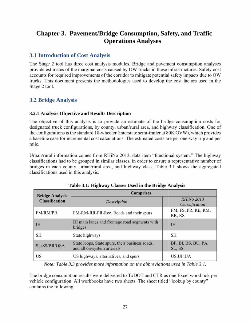
The objective of this analysis is to provide an estimate of the bridge consumption costs for designated truck configurations, by county, urban/rural area, and highway classification. One of the configurations is the standard 18-wheeler (interstate semi-trailer at 80K GVW), which provides a baseline case for incremental cost calculations. The estimated costs are per one-way trip and per mile. Urban/rural information comes from RHiNo 2013, data item “functional system.” The highway classifications had to be grouped in similar classes, in order to ensure a representative number of bridges in each county, urban/rural area, and highway class. Table 3.1 shows the aggregated classifications used in this analysis.

Table 3.1: Highway Classes Used in the Bridge Analysis

Bridge Analysis Classification

Comprises

Description RHiNo 2013

Classification

FM/RM/PR FM-RM-RR-PR-Rec. Roads and their spurs FM, FS, PR, RE, RM, RR, RS

IH IH main lanes and frontage road segments with bridges

IH

SH State highways SH

SL/SS/BR/OSA State loops, State spurs, their business roads, and all on-system arterials

BF, BI, BS, BU, PA, SL, SS

US US highways, alternatives, and spurs US,UP,UA

Note: Table 3.3 provides more information on the abbreviations used in Table 3.1. The bridge consumption results were delivered to TxDOT and CTR as one Excel workbook per vehicle configuration. All workbooks have two sheets. The sheet titled “lookup by county” contains the following:

28

1. The first two columns of Table 3.1 above,

2. A sketch of the truck configuration,

3. The percentage of bridges statewide exceeding the operating rating for that configuration, and

4. A summary (pivot) table where the user can select a county and retrieve the configuration’s bridge consumption cost per mile per (one-way) trip.

Figure 3.1 provides a screen capture of the summary table for Bexar County. It is very important to note two Excel pivot table features:

1. Some new versions of Excel no longer automatically update the pivot table after selecting a new option; it may be necessary to refresh it every time a new county is selected.

2. The Excel pivot table gives correct results ONLY for each county. Choosing the option “all” DOES NOT give correct statewide results, due to the way Excel automatically calculates pivot tables. If the user desires results aggregated in any way other than county (such as TxDOT District or statewide), s/he should go to the data sheet with complete results (discussed next).

Figure 3.1. Screen Capture of the Data Summary by County

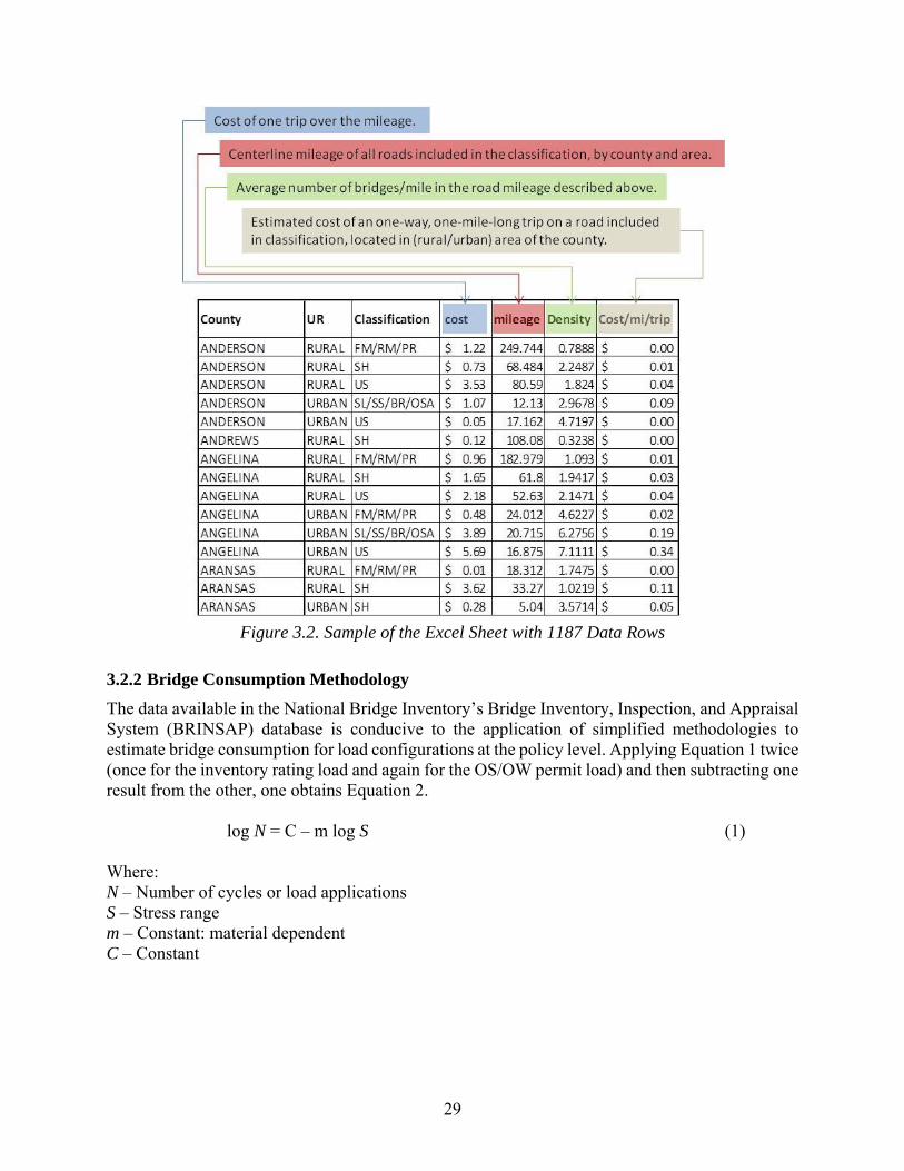
The other sheet in each workbook is titled after the configuration number. It contains a table with 1187 data rows and a sketch of the vehicle configuration. Figure 3.2 shows a partial screen capture of the data with a detailed explanation of the data columns. The cost of any specific one-way route can be estimated by multiplying the unit cost by the route mileage, taking care to match highway class, and urban/rural area. For round trip, double the cost. If a route contains a segment with multiple highway classifications, the highest classification should be utilized. If a new road with a previously non-existent classification is being considered, use the estimates by urban area and region (east or west Texas) for that highway class. When estimating a route cost, is important to assign each route segment to its proper urban or rural area. The average costs generally are considerably different due to the higher bridge density in urban areas.

Select county BEXAR

Cost/mile/trip AreaClassification RURAL URBANFM/RM/PR 0.02$ 0.03$ IH 0.07$ 0.74$ SH 0.06$ 0.29$ SL/SS/BR/OSA 0.03$ 0.15$ US 0.03$ 0.49$

29

Figure 3.2. Sample of the Excel Sheet with 1187 Data Rows

3.2.2 Bridge Consumption Methodology

The data available in the National Bridge Inventory’s Bridge Inventory, Inspection, and Appraisal System (BRINSAP) database is conducive to the application of simplified methodologies to estimate bridge consumption for load configurations at the policy level. Applying Equation 1 twice (once for the inventory rating load and again for the OS/OW permit load) and then subtracting one result from the other, one obtains Equation 2.

log N = C – m log S (1) Where: N – Number of cycles or load applications S – Stress range m – Constant: material dependent C – Constant

30

(2) Where: Ninventory – Number of load applications for the inventory rating load NOSOW – Number of load applications for the OS/OW load Sinventory – Stress range for the inventory load SOSOW – Stress range for the OS/OW load m – Constant: material dependent At the policy level, it is not feasible to calculate actual stress ranges for bridge details. Digital descriptions of bridge cross sections and other characteristics are not available; even if they were, computational demands would make this task unfeasible within this project’s time frame. An acceptable method successfully used in previous OS/OW studies involves using live load bending moments as surrogates for the stress range (Imbsen et al., 1987; Weissmann & Harrison, 1992; and Weissmann, et al., 2002). This approach substitutes the stress ranges in Equation 2 with bending moments, defining the bridge consumption ratio as depicted in Equation 3. Simply put, Equation 3 states that the bridge consumption ratio induced by a bending moment of an inventory rating load passage on a given bridge is equal to 1. Loads inducing bending moments twice as large as the inventory rating bending moment lead to a bridge consumption ratio of two to the power “m”, where “m” is a function of the bridge material. Altry et al., 2003 and Overman et al., 1984, recommend “m” values that can be matched to the corresponding BRINSAP structure type codes.

(3) Where: Minventory – Live load bending moment for the inventory rating load MOSOW – Live load bending moment for the OS/OW load m – Constant: material dependent The bridge consumption in dollars due to the passage of a given load is estimated by using Equation 3 combined with a consumable asset value for the bridge. The recently completed Federal Truck Size and Weight study recommends that the current asset value of a bridge is $235 per square foot of deck area. Previous highway cost allocation studies established that the asset value of a bridge should be allocated according to Table 3.2, with 11 percent of the bridge asset value attributable to loads that are over HS20-44 (FHWA, 2000). HS20-44 is a standardized bridge design load, and current bridge inventory ratings are usually represented as multiples of the HS20 design load when recorded in BRINSAP.

mInventory

mOSOW

OSOW

Inventory

S

S

NN =

MMnRatioConsumptio

m

Inventory

OSOW=

31

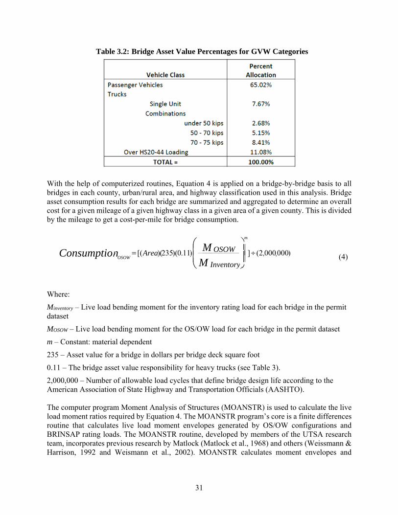
Table 3.2: Bridge Asset Value Percentages for GVW Categories

With the help of computerized routines, Equation 4 is applied on a bridge-by-bridge basis to all bridges in each county, urban/rural area, and highway classification used in this analysis. Bridge asset consumption results for each bridge are summarized and aggregated to determine an overall cost for a given mileage of a given highway class in a given area of a given county. This is divided by the mileage to get a cost-per-mile for bridge consumption.

(4)

Where:

Minventory – Live load bending moment for the inventory rating load for each bridge in the permit dataset

MOSOW – Live load bending moment for the OS/OW load for each bridge in the permit dataset

m – Constant: material dependent

235 – Asset value for a bridge in dollars per bridge deck square foot

0.11 – The bridge asset value responsibility for heavy trucks (see Table 3).

2,000,000 – Number of allowable load cycles that define bridge design life according to the American Association of State Highway and Transportation Officials (AASHTO). The computer program Moment Analysis of Structures (MOANSTR) is used to calculate the live load moment ratios required by Equation 4. The MOANSTR program’s core is a finite differences routine that calculates live load moment envelopes generated by OS/OW configurations and BRINSAP rating loads. The MOANSTR routine, developed by members of the UTSA research team, incorporates previous research by Matlock (Matlock et al., 1968) and others (Weissmann & Harrison, 1992 and Weismann et al., 2002). MOANSTR calculates moment envelopes and

)000 ,000,2(])11.0)(235)([( ÷=

MMn Consumptio

Inventory

OSOWArea

m

OSOW

32

identifies the maximum live load bending moments (positive and negative) induced by the OS/OW configuration and the inventory rating load.

3.2.3 Data Preparation

The steps listed below summarize the data preparation that was necessary to obtain mileages, assign a consistent highway classification as well as urban/rural area to each bridge, and arrive at the cost results previously discussed.

Step 1: Assign a consistent urban/rural classification to each bridge.

First, urban/rural classifications were retrieved from both RHiNo and BRINSAP, using their functional system variables. Urban/rural classification using the “functional_system” RHiNo variable does always not match the urban/rural classification using BRINSAP’s equivalent variable, described in item 26/26A of the coding guide. It was necessary to manually resolve all inconsistencies.

Step 2: Develop a highway classification system that is consistent with RHiNo and BRINSAP.

The research team needed to assign a RHiNo classification to each bridge. As depicted in Table 3, highway classifications in RHiNo do not always match those used in BRINSAP (items 5.2 or 5.2A, depending on whether the bridge is located on the inventory route or passes under it). Every time the two classifications did not match, the bridge was assigned the same classification as the RHiNo segment where each it is located. Once each bridge had a RHiNo classification, the following was done:

1. Using RHiNo, determine the total centerline mileage within each county and urban/rural area for each highway classification.

2. Using BRINSAP and the RHiNo highway classification of each bridge, determine the number of bridges in each county, urban/rural area, and each RHiNo highway classification.

3. Not every area in each county actually had bridges in each RHiNo classification; thus, it was necessary to aggregate some classifications to ensure meaningful results. These final aggregated classifications were listed in Table 3.3.

33

Table 3.3: RHiNo and BRINSAP On-System Highway Classifications

RHiNo Variable

Value

RHiNo Highway Classification

BRINSAP Variable

Value

BRINSAP Variable Description

Closest Classification to

RHiNo’s

BF Business FM 28 Business F.M. Hwy BF

BI Business IH 25 Business Interstate BI

BS Business SH 27 Business S.H. Hwy BS

BU Business US 26 Business U.S. Hwy BU

FM FM 15 Farm or Ranch to Market Road

FM/RM

FS FM Spur

IH IH 11 Interstate Highway IH

PA Principal Arterial

PR Park Road 16 Park Road PR

RE Recreational Road 17 Recreational Road/Spur

RE

RM RM 15 Farm or Ranch to Market Road

FM/RM

RR Ranch Road

RS RM Spur

SH SH 13 State Highway SH

SL SL 14 State Loop or Spur SL/SS

SS State Spur 14 State Loop or Spur SL/SS

UA US Alt.

UP US Spur 12 US Highway (Spur) US (Spur)

US US 12 US Highway (Spur) US (Spur) 20 Toll Road

51 State Lands Road

19/99 Other

24 NASA1

41 Federal Lands Rd

Step 3: Identify and eliminate from the analysis parallel bridges, culverts, and tunnels.

BRINSAP has variables identifying these situations. Culverts and tunnels are straightforward, and so is travel direction. However, an additional data treatment was necessary to eliminate parallel bridges in the same traffic direction, which are often present. BRINSAP item 101 was used but several cases had to be manually checked in online maps and pictures using the geographical coordinates of the bridge. The data treatment to eliminate all parallel bridges was necessary due to the nature of the RHiNo data reporting centerline mileage. If calculating the consumption due to

34

one truck pass, considering more than one parallel bridge in the same location would artificially increase the cost; the truck consumes only one of the bridges in each pass.

Step 4: Calculate the bridge consumption of all on-system bridges.

The previous steps resulted in an analysis database with all pertinent BRINSAP variables, the aggregated highway classification developed as described in step 2, an urban/rural area consistent with RHiNo, and no parallel structures or structures other than on-system bridges. This database was used to calculate the moment ratio and costs for each bridge, which were then added up by highway classification, area type, and county, to obtain the final results reported in the spreadsheets previously discussed (see Figure 3.1 and Figure 3.2). The costs were also added up by highway classification, urban/rural, and Texas region (east/west) for use in planned or new highways with a classification that was previously nonexistent in the desired county.

3.2.4 Conclusions

The product of this analysis is a network-level bridge consumption cost per vehicle miles traveled by county, urban/rural area, and the aggregated highway class depicted in Table 3.3, for each of the configurations of interest. It provides a useful tool to estimate the bridge consumption costs of proposed configurations for any given route in any county. Nevertheless, such estimates are less accurate than a project-level analysis of specific routes or corridors, basically for two reasons:

1. A corridor or route analysis calculates each specific bridge consumption cost rather than use average costs by factorial cells, and

2. The network-level analysis presented here depends on averages by highway class, area, and county, which in turn required resolving some inconsistencies among RHiNo and BRINSAP based on network-level type of reasoning and/or judgment, as previously discussed. This does not occur in a route-specific analysis where each individual bridge is considered. On the other hand, this analysis is not tied up to specific routes or highways and its results can be used statewide.

3.3 Pavement Analysis

3.3.1 Background

During the Rider 36 study [Prozzi et al. 2012], CTR evaluated OS/OW load permits issued by the Motor Carrier Division of the TxDMV. A pavement consumption analysis methodology was developed during Rider 36 considering that these loads might exceed either the Texas legal axle load limits or total GVW. The Rider 36 pavement consumption methodology were used as a basis to evaluate OS/OW loads operating at port and border-port-of entry OS/OW corridors. This document presents a methodology for establishing equivalencies between OW loads based on the concept of “equivalent consumption” to the pavement structure using mechanistic-empirical pavement analysis procedures. In the proposed methodology, each pavement section is evaluated using three different distress criteria: (1) surface deformation or rutting, (2) load-associated fatigue cracking, and (3) riding quality in terms of roughness (International Roughness Index, IRI). The methodology proposed here represents a significant enhancement over previous procedures in the sense that it allows the analyst to adopt a modular approach towards calculation of the overall load

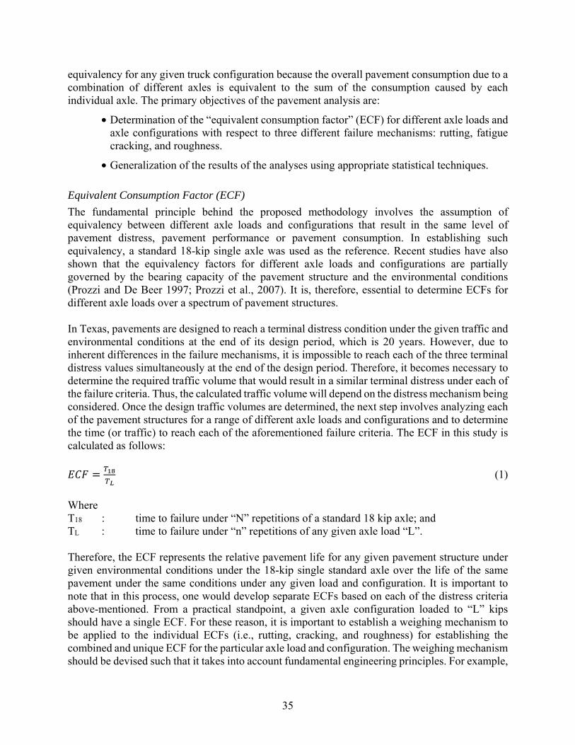
35

equivalency for any given truck configuration because the overall pavement consumption due to a combination of different axles is equivalent to the sum of the consumption caused by each individual axle. The primary objectives of the pavement analysis are:

• Determination of the “equivalent consumption factor” (ECF) for different axle loads and axle configurations with respect to three different failure mechanisms: rutting, fatigue cracking, and roughness.

• Generalization of the results of the analyses using appropriate statistical techniques.

Equivalent Consumption Factor (ECF)

The fundamental principle behind the proposed methodology involves the assumption of equivalency between different axle loads and configurations that result in the same level of pavement distress, pavement performance or pavement consumption. In establishing such equivalency, a standard 18-kip single axle was used as the reference. Recent studies have also shown that the equivalency factors for different axle loads and configurations are partially governed by the bearing capacity of the pavement structure and the environmental conditions (Prozzi and De Beer 1997; Prozzi et al., 2007). It is, therefore, essential to determine ECFs for different axle loads over a spectrum of pavement structures. In Texas, pavements are designed to reach a terminal distress condition under the given traffic and environmental conditions at the end of its design period, which is 20 years. However, due to inherent differences in the failure mechanisms, it is impossible to reach each of the three terminal distress values simultaneously at the end of the design period. Therefore, it becomes necessary to determine the required traffic volume that would result in a similar terminal distress under each of the failure criteria. Thus, the calculated traffic volume will depend on the distress mechanism being considered. Once the design traffic volumes are determined, the next step involves analyzing each of the pavement structures for a range of different axle loads and configurations and to determine the time (or traffic) to reach each of the aforementioned failure criteria. The ECF in this study is calculated as follows: = (1)

Where T18 : time to failure under “N” repetitions of a standard 18 kip axle; and TL : time to failure under “n” repetitions of any given axle load “L”. Therefore, the ECF represents the relative pavement life for any given pavement structure under given environmental conditions under the 18-kip single standard axle over the life of the same pavement under the same conditions under any given load and configuration. It is important to note that in this process, one would develop separate ECFs based on each of the distress criteria above-mentioned. From a practical standpoint, a given axle configuration loaded to “L” kips should have a single ECF. For these reason, it is important to establish a weighing mechanism to be applied to the individual ECFs (i.e., rutting, cracking, and roughness) for establishing the combined and unique ECF for the particular axle load and configuration. The weighing mechanism should be devised such that it takes into account fundamental engineering principles. For example,

36

it is known that rutting is more critical in warm climatic regions, while cracking is the dominant distress mechanism in colder climatic regions.

3.3.2 Mechanistic-Empirical Pavement Analysis

For the mechanistic analysis, it was decided to use the newly developed AASHTOWare ME Pavement Design for analysis and computation of pavement distresses resulting from the imposed traffic (ARA, 2008). The AASHTOWare uses the same mechanistic-empirical concepts as its predecessor, the Mechanistic-Empirical Pavement Design Guide developed under the National Cooperative Highway Research Program. The methodology has been approved by AASHTO and supported by the Federal Highway Administration (FHWA). In mechanistic-empirical pavement analysis, the fundamental pavement responses under repeated traffic loadings are calculated using a multi-layer linear elastic approach. This approach assumes that a flexible pavement is a multi-layered structure and that each of the layers exhibit a linearly elastic response to traffic loads. Although this is not the case, the linearity assumption is reasonable at the low strain levels typical of highway traffic. The method computes the stresses and strains that are induced in the pavement layers due to traffic loadings. These critical pavement responses are then related to field distresses using empirical relationships, which are calibrated based on field observations.

Experimental Design

The ECF for any given axle load and configuration is expected to be a function of the structural capacity of the highway facility (Prozzi et al., 2007; Kinder, 2008). Besides, environmental conditions determine several site features including the climatic profile and type of subgrade support which in turn have a bearing on the pavement response and performance that is typically built in a given region. For these reasons, it is important to design an experiment that encompasses different pavement structures, traffic levels and climatic regions. Permitted load configurations do not necessarily conform to typical legal limits that are placed on highway vehicles. Due to the nature of the payload, these vehicles can have atypical axle configuration as well as axle loads. This aspect led the study team to simulate a wide range of axle loads with different configuration such that the full axle spectra for OW loads can be characterized. Table 3.4 summarizes the range of axle loads and configurations that were included as part of this study. Contact stress (assumed to be equal to the tire inflation pressure) was restricted to 120 psi for all possible combinations of axle loads and configurations.

37

Table 3.4: Simulated Axle Loads and Configurations

Axle Configuration

Axle Loads (in kips)

Single Tandem Tridem Quad 8 18 30 30 10 22 36 36 12 26 42 42 14 30 48 48 16 34 54 54 18 38 60 60 20 42 66 66 22 46 72 72 24 50 78 78

3.3.3 Analysis Results

Determination of ECF for Rutting

It is possible to establish an approximated linear relationship between the ECF and the normalized axle load on a log-log scale. As an example, Figure 3.3 shows that there is a strong linear relationship between these two variables.

Figure 3.3 EDFs based on Rutting Criterion

The slope of the line differs slightly for all pavement sections and this indicates that the ECF for any given axle load and configurations is influenced by the pavement material properties, structural capacity of the highway and the environmental conditions. For the case of tandem and tridem axles, the study team introduced the group equivalency factor (GEF) in establishing the ECF. The following generalized expression was used to estimate the ECF for any given axle load and configuration while using the rutting failure criteria: ( ) = × = × × (2)

Where α = Axle Load Factor (ALF) β = Group Equivalency Factor (GEF)

38

It was established that the axle load factor (ALF) is quite consistent for a given pavement structure and hardly changes for the different axle groups. Based on the literature, ALFs are expected to be a function of the structural capacity of the pavement structures. This would imply that the ALF should exhibit high correlation with the structural number (SN), as the GEF is optimized, such that it gives the best linear predictor between the ECF and the normalized load in a log-log scale for all pavement sections included in this study. Figure 3.4 represents the correlation between ALFs and pavement structural capacity as represented by its SN. It is between axles.

(a) Single

(b) Tandem

(c) Tridem

Figure 3.4 Relation between ALF and SN based on Rutting

39

Determination of ECF for Fatigue Cracking

The calculation of ECF for fatigue cracking was undertaken using the same approach as for rutting. As an example, Figure 3.5 shows the relationship between the normalized loads and the ECF on a log-log scale.

(a) Single Axles

(b) Single Axles

(c) Single Axles

Figure 3.5 ECFs based on Fatigue Criterion

Once again, it was observed that the calculated ALF follow a similar pattern for different axle configurations for different pavement sections. It is important to note that the rutting and fatigue cracking transfer functions, which are used in the mechanistic analysis, have similar specification forms which explains why the relationship between these two variables has similar characteristics.

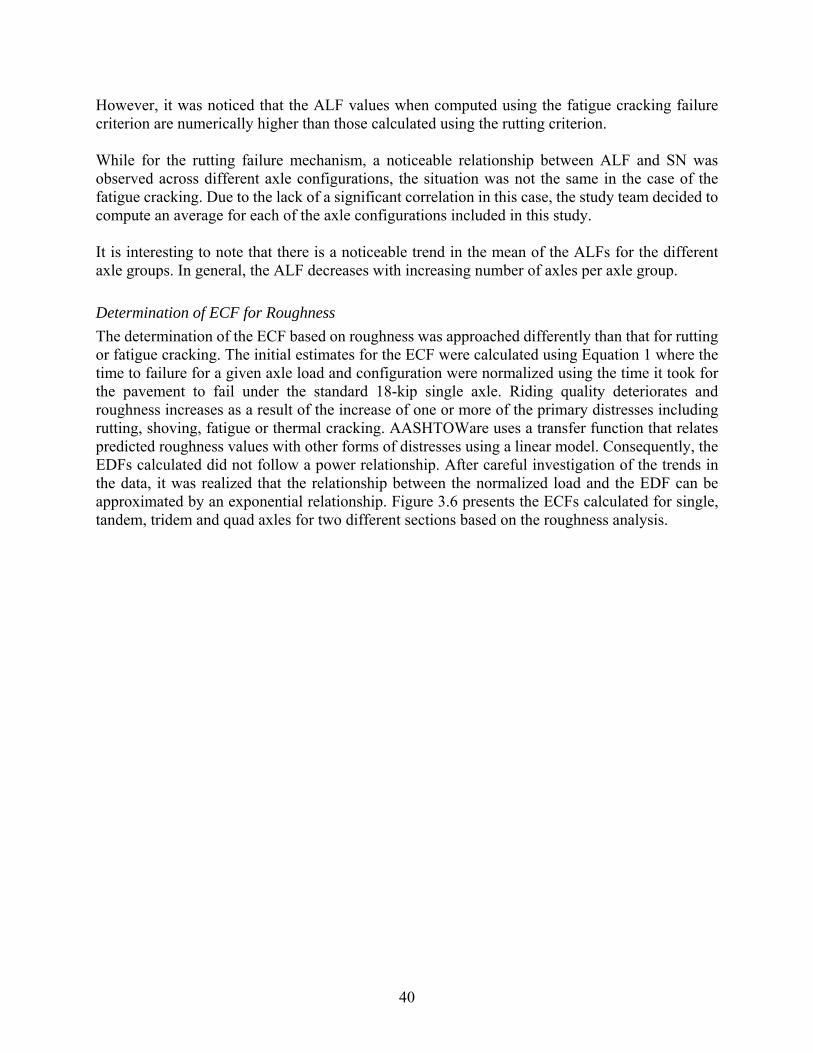
40

However, it was noticed that the ALF values when computed using the fatigue cracking failure criterion are numerically higher than those calculated using the rutting criterion. While for the rutting failure mechanism, a noticeable relationship between ALF and SN was observed across different axle configurations, the situation was not the same in the case of the fatigue cracking. Due to the lack of a significant correlation in this case, the study team decided to compute an average for each of the axle configurations included in this study. It is interesting to note that there is a noticeable trend in the mean of the ALFs for the different axle groups. In general, the ALF decreases with increasing number of axles per axle group.

Determination of ECF for Roughness

The determination of the ECF based on roughness was approached differently than that for rutting or fatigue cracking. The initial estimates for the ECF were calculated using Equation 1 where the time to failure for a given axle load and configuration were normalized using the time it took for the pavement to fail under the standard 18-kip single axle. Riding quality deteriorates and roughness increases as a result of the increase of one or more of the primary distresses including rutting, shoving, fatigue or thermal cracking. AASHTOWare uses a transfer function that relates predicted roughness values with other forms of distresses using a linear model. Consequently, the EDFs calculated did not follow a power relationship. After careful investigation of the trends in the data, it was realized that the relationship between the normalized load and the EDF can be approximated by an exponential relationship. Figure 3.6 presents the ECFs calculated for single, tandem, tridem and quad axles for two different sections based on the roughness analysis.

41

(a) Section 1, single axle

(b) Section 1, tandem axle

(c) Section 1, tridem axle

Figure 3.6 EDFs based on Roughness Criterion

Following is the relationship that was used to relate the EDFs calculated using the roughness failure criteria with the normalized load: ln ( ) = × × − 1 (3)

While in the case of rutting and fatigue cracking, it was seen that there is a strong linear relationship between the GEFs and the number of axles in the axle group, the same was not the case for those calculated using the roughness criteria. In fact, it was noticed that a power law can relate the GEF to the number of axles in the group (see Figure 3.7).

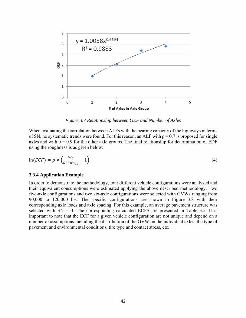
42

Figure 3.7 Relationship between GEF and Number of Axles

When evaluating the correlation between ALFs with the bearing capacity of the highways in terms of SN, no systematic trends were found. For this reason, an ALF with ρ = 0.7 is proposed for single axles and with ρ = 0.9 for the other axle groups. The final relationship for determination of EDF using the roughness is as given below: ln ( ) = × × − 1 (4)

3.3.4 Application Example

In order to demonstrate the methodology, four different vehicle configurations were analyzed and their equivalent consumptions were estimated applying the above described methodology. Two five-axle configurations and two six-axle configurations were selected with GVWs ranging from 90,000 to 120,000 lbs. The specific configurations are shown in Figure 3.8 with their corresponding axle loads and axle spacing. For this example, an average pavement structure was selected with SN = 3. The corresponding calculated ECFS are presented in Table 3.5. It is important to note that the ECF for a given vehicle configuration are not unique and depend on a number of assumptions including the distribution of the GVW on the individual axles, the type of pavement and environmental conditions, tire type and contact stress, etc.

43

(a) Class 9: 90,000 GVW (b) Class 9: 105,000 GVW

(c) Class 10: 114,000 GVW (d) Class 10, 120,000 GVW

Figure 3.8 Vehicle Analyzed Vehicle Configurations

Table 3.5: Equivalent Consumption Factors for Analyzed Vehicles

Vehicle Configuration ECF

Class 9 @ 90,000 lbs GVM 7.01

Class 9 @ 105,000 lbs GVM 12.24

Class 10 @ 114,000 lbs GVM 10.83

Class 10 @ 120,000 lbs GVM 11.90

3.3.5 Cost Allocation

While trying to develop a permit fee structure based on the equivalent consumption approach, it is important to realize the economic benefit that the trucking industry brings to the state. It is also essential to ensure that the permit fees assessed on OW vehicles is commensurate with the imposed additional infrastructure consumption. The permit fee structure suggested as part of this study is based on consumption of the service life of the highway infrastructure by OW truck traffic and no attempts have been made to account for the economic benefits of increasing axle loads. This was out of the original scope of the study reported in this document. Highway construction costs are allocated to road users based on cost allocation studies that have been conducted at federal and state level. In cost allocation, there are three basic requirements: marginality, completeness and rationality. There are several approaches for allocating highway construction costs to the responsible parties. Among these, the most widely used methodologies are (i) the Incremental Method, (ii) the Proportional Method, and (iii) the Modified Incremental Method.

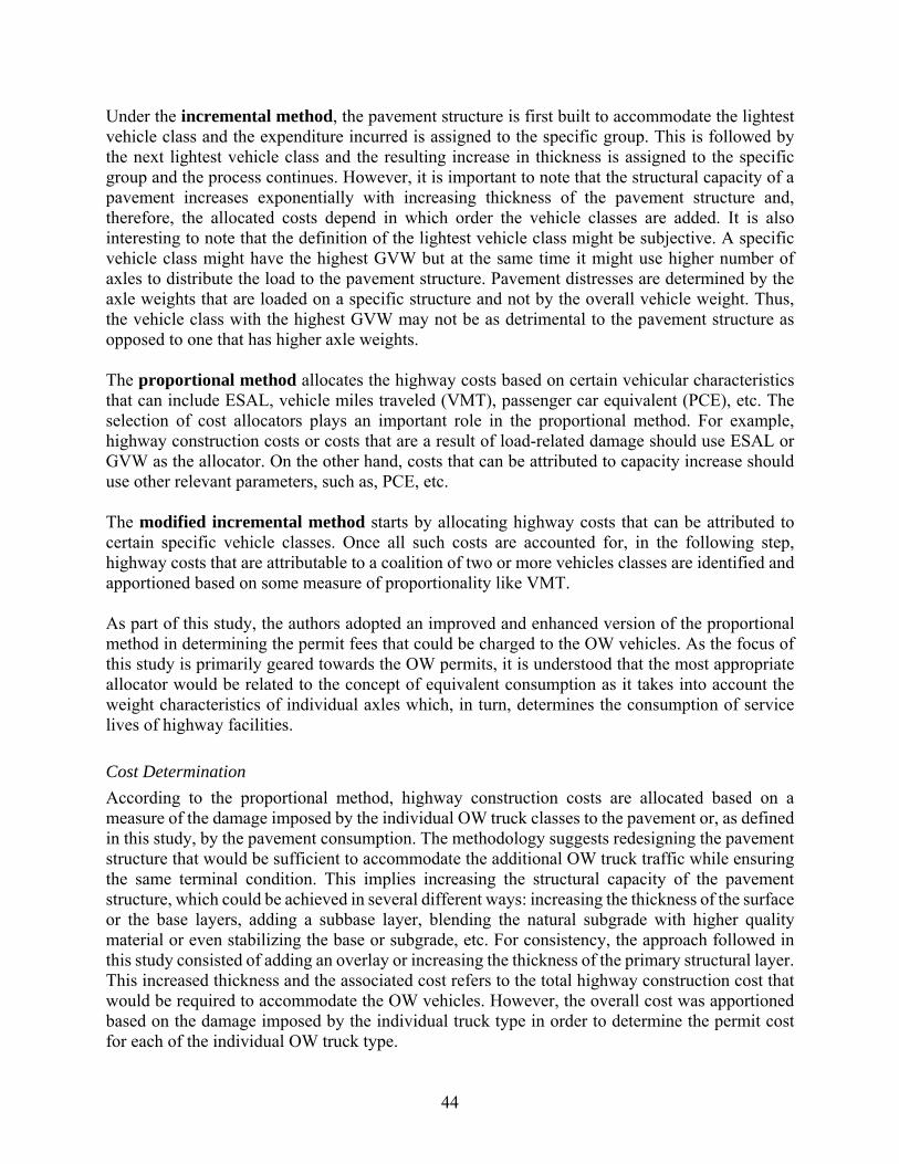
44

Under the incremental method, the pavement structure is first built to accommodate the lightest vehicle class and the expenditure incurred is assigned to the specific group. This is followed by the next lightest vehicle class and the resulting increase in thickness is assigned to the specific group and the process continues. However, it is important to note that the structural capacity of a pavement increases exponentially with increasing thickness of the pavement structure and, therefore, the allocated costs depend in which order the vehicle classes are added. It is also interesting to note that the definition of the lightest vehicle class might be subjective. A specific vehicle class might have the highest GVW but at the same time it might use higher number of axles to distribute the load to the pavement structure. Pavement distresses are determined by the axle weights that are loaded on a specific structure and not by the overall vehicle weight. Thus, the vehicle class with the highest GVW may not be as detrimental to the pavement structure as opposed to one that has higher axle weights. The proportional method allocates the highway costs based on certain vehicular characteristics that can include ESAL, vehicle miles traveled (VMT), passenger car equivalent (PCE), etc. The selection of cost allocators plays an important role in the proportional method. For example, highway construction costs or costs that are a result of load-related damage should use ESAL or GVW as the allocator. On the other hand, costs that can be attributed to capacity increase should use other relevant parameters, such as, PCE, etc. The modified incremental method starts by allocating highway costs that can be attributed to certain specific vehicle classes. Once all such costs are accounted for, in the following step, highway costs that are attributable to a coalition of two or more vehicles classes are identified and apportioned based on some measure of proportionality like VMT. As part of this study, the authors adopted an improved and enhanced version of the proportional method in determining the permit fees that could be charged to the OW vehicles. As the focus of this study is primarily geared towards the OW permits, it is understood that the most appropriate allocator would be related to the concept of equivalent consumption as it takes into account the weight characteristics of individual axles which, in turn, determines the consumption of service lives of highway facilities.

Cost Determination

According to the proportional method, highway construction costs are allocated based on a measure of the damage imposed by the individual OW truck classes to the pavement or, as defined in this study, by the pavement consumption. The methodology suggests redesigning the pavement structure that would be sufficient to accommodate the additional OW truck traffic while ensuring the same terminal condition. This implies increasing the structural capacity of the pavement structure, which could be achieved in several different ways: increasing the thickness of the surface or the base layers, adding a subbase layer, blending the natural subgrade with higher quality material or even stabilizing the base or subgrade, etc. For consistency, the approach followed in this study consisted of adding an overlay or increasing the thickness of the primary structural layer. This increased thickness and the associated cost refers to the total highway construction cost that would be required to accommodate the OW vehicles. However, the overall cost was apportioned based on the damage imposed by the individual truck type in order to determine the permit cost for each of the individual OW truck type.

45

The study team considered the scenario where the total number of ESALs owing to the OW vehicles equals that of the design traffic volume. However, designing the pavement structure to cater to the OW truck volume only was not considered as it would be inappropriate because the highway facility was designed for the design traffic only. Therefore, the OW traffic was added to the design traffic volume. The additional traffic volume implies increased structural capacity which would be provided through additional thickness and the associated costs would be apportioned to the total number of OW trucks. In summary, the methodology used in calculation of the pavement costs due to OW vehicles considered providing additional structural capacity to the highway facility and calculated any costs thus incurred. A key component of the entire procedure involved obtaining reliable estimates for construction costs. The particular objective was addresses by referring to TxDOT’s average low bid price portal which provided the study team with unit cost for each of the different materials. The unit costs were multiplied with the total quantity of material that would be required to provide the additional structure required to support the OW traffic. The calculated costs were determined in terms of dollar/ESAL/mile. Figure 3.9 provides information on the calculated costs on each of the individual flexible and rigid pavement sections using the different distress mechanisms considered in this study.

Pavement Rutting Pavement Roughness

Figure 3.9 Pavement Costs Assessed for OW Vehicles based in 2011 values

The study team realized that there was hardly any relationship between the calculated fees and the functional classification or the SN for a given highway facility. The particular finding encouraged the authors to obtain an average fee irrespective of the highway facility.

3.4 Safety Project Analysis

The Stage 2 Tool has the option to include safety projects if the user requires it. These costs are included in the truck permit fee estimation. These costs might include upgrading an intersection or adding traffic signals, a right- or left-turn bay, or other treatment that improves safety and traffic operations while considering OW trucks operating in mixed traffic.

3.4.1 Process of Cost Estimation

The user needs to estimate the cost of the safety projects in order to include it in the analysis; this need arises from two factors:

46

• The project cost varies considerably among the different counties and TxDOT Districts.

• The user would have more knowledge about local conditions and project-level details. These costs are included in the analysis, and split evenly among the estimated OW trucks that will use the corridor. The resulting value is added to the permit fee estimated for pavement and bridge consumption. Nevertheless, the Stage 2 tool will provide seven reference values for safety projects. Table 3.6 presents the sample included in Stage 2. This sample came from analyzing safety projects in Texas from 2009 to 2015 excluding the joint projects (for example, projects that contained installing light signals and improving the pavement of the intersection). Values are in 2014 dollars.

Table 3.6: Mean Costs of Safety Projects

Item Unit Cost Number of Projects

in the Database

Add Turn Lanes Global $379,000 77

Install Traffic Signals Global $170,000 74

Extend Culverts Global $60,000 1

Widen 3 ft Center-Mile $910,000 6

Widen 10 ft Center-Mile $1,165,000 3

Install Guardrail Center-Mile $49,000 51

Install Flashing Beacon Global $64,000 72 These costs are provided only as reference values. To increase the estimation’s accuracy, the user should always estimate the cost for each specific project.

3.5 Chapter 3 References

Altry, A.K., Arabbo, D.S., Crowin, E.B., Dexter, R.J., and French, C.E., (2003). “Effects of increasing truck weight on steel and prestressed bridges”, Mn/DOT final report (2003-16), Minnesota Department of Transportation. Imbsen, R.A. and R.A. Schomber. Simplified Bridge Load Rating Methodology Using the National Bridge Invento-ry File, Arizona Department of Transportation, August 1987. Matlock, H. and Taylor, T., “A Computer Program to Analyze Beam-columns Under Movable Loads”, Research Project 3-5-63-56. Center for Transpiration Research, University of Texas at Austin, Austin, TX. Weissmann, J., and R. Harrison, “The Impact of Turnpike Doubles and Triple 28s on the Rural Interstate Bridge Network,” Transportation Research Record 1319, TRB, National Research Council, 1992.

47

Weissmann J., R. Harrison and M. Diaz, A Computerized Model to Evaluate the Impacts of Truck Size and Weight Changes on Bridges, First International Conference on Bridge Maintenance, Safety and Management, IABMAS 2002, Barcelona, 14-27, July, 2002 Overman T.R., Breen J.E., and Frank K.H. (1984). “Fatigue Behavior of Pretensioned Concrete Girders”. Final Research Report 300-2F. Center for Transportation Re-search, Bureau of Engineering Research, University of Texas at Austin, Austin, TX. United States Department of Transportation, Comprehen-sive Truck Size and Weight (CTS&W) Study, FHWA, 2000 (at http://www.fhwa.dot.gov/reports/tswstudy/index.htm. Texas Department of Transportation. Oversize/Overweight Permit Rules and Regulations – 43 Texas Administrative Code Chapters 28, Subchapters A-K. Published by the Texas Department of Transportation – Motor Carrier Division – 4203 Bull Creek, Austin, TX 78731, January, 2011a. Prozzi, J.A. and M. De Beer (1997). Mechanistic Determination of Equivalent Damage Factors for Multiple Load and Axle Configurations, Proceedings of the 8th International Conference on Asphalt Pavements, Vol. 1, pp. 161-177, Seattle, WA, August 10-14, 1997. Prozzi, J.A., F. Hong, and S. Grebenschikov. Equivalent Damage Factors Based on Mechanistic-Empirical Pavement Design. CD ROM Proceedings of the 86th Annual Meeting of the Transportation Research Board, Washington, D.C., January 21-25, 2007. Kinder, D. F., & M. G. Lay (1988). Review of the fourth power law. ARRB, Internal Report # AIR000-248. Applied Research Associates (2008), Mechanistic-Empirical Pavement Design Guide, Interim Edition: A Manual of Practice, ISBN Number: 1-56051-423-7.

48

Chapter 4. Development of Stage 2 Prototype Detailed Analysis Tool

4.1 Introduction of Stage 2 Prototype Detailed Analysis Tool

In the Stage 2 prototype detailed analysis tool are two “archived” corridors—the Port of Brownsville and Hidalgo County RMA OS/OW corridors—with two truck configurations. The final Stage 2 tool has 12 different truck configurations and space for up to 13 more truck configurations if required in the future (25 in total). These additional truck configurations will be implemented in in the tool in subsequent tasks. This document presents the general process of the Stage 2 prototype tool, providing screenshots of each step.

4.2 General Process of Stage 2 Tool

The user input modules consist of three levels: Corridor Network Level, Route Level, and Segment Level, as discussed in Chapter 2. In the Corridor Network Level module, the user’s input consists of basic corridor information (e.g., corridor name), OW traffic information (e.g., the number of trucks in the first year of operation), and permit information (if available). The specific information needed is summarized in Table 4.1.

Table 4.1: Input for Corridor Network Attributes Corridor Network Level Inputs

General Corridor Information

OW Traffic Information Permit Information

Corridor Name Estimated OW Trucks in the

First Year of Analysis Current Permit Fee

Corridor Comments Annual Growth Rate Deduction Agency 1

Percentage of Trucks Following Configuration 1

Percentage of the Fee for Agency 1

Percentage of Trucks Following Configuration 2

Deduction Agency 2

… Percentage of the Fee for

Agency 2

… In the Route Level module, the user will need to input the road characteristics. Following are the specific attributes at the route level:

1. Route functional class posted.

2. Route number (for example, if it is State Highway 48, it should be “48”).

49

3. Route comments (anything the user wants to store about the route, such as “This is a new corridor”).

The Segment Level module allows for accurate estimation of a complete route, as it breaks the route into segments based on certain consumption factors. Because the pavement consumption cost and the bridge consumption cost vary according to these different factors, routes in the network have to be segmented accordingly. For example, the same route could contain some sections paved with asphalt concrete pavement (ACP), some with jointed concrete pavement (JCP), or even continuously reinforced concrete pavement (CRCP). These sections need to be identified as separate segments, in order to accurately estimate the pavement consumption cost. This module defines the segments in a route by five criteria:

1. If there is change in pavement materials, the route should be divided into different segments. Pavement material type will impact the pavement consumption analysis.

2. If a route goes through both rural and urban areas, it should be divided into different segments. The bridge consumption differs between rural and urban areas.

3. If there is an intersection on the route where OW trucks can be diverted, the route should be segmented at that intersection. The intersection will change the OW truck traffic, which leads to a different consumption result, as Figure 4.1 indicates.

Figure 4.1: Example of OW Truck Diversion at an Intersection

4. If a route goes through different counties, it should be divided into different segments by county line. The bridge consumption varies from county to county.

5. If the number of lanes in the roadbed changes, the route should be segmented accordingly. The pavement consumption costs are applied to the lanes that are part of the roadbed.

Based on the route segmentation criteria, the following information will be needed for each segment: pavement type, location type (urban/rural), county, number of lanes in the roadbed, and centerline miles.

SH XX

FM YY

100% 50%

50%

50

4.3 Estimations of Consumption Costs

4.3.1 Estimation of Pavement Consumption

Table 4.2 summarizes the inputs, processes, and outputs of pavement consumption estimation.

Table 4.2: Estimation of Pavement Consumption

Steps Inputs Process Outputs

1 • Pavement type (ACP, JCP,

and CRCP) • Truck configuration

Search for the consumption factor based on the input

Pavement consumption factor per truck configuration

2 Number of lanes of the roadbed (of each segment)

Multiply the consumption factor found in (1) and the number of lanes

Consumption cost per VMT per truck configuration

3

• Number of trucks in the segment per each truck configuration

• Centerline miles

Multiply (2) and the number of trucks that have that specific truck configuration, and then multiply that figure by centerline miles

Pavement consumption cost for that segment per truck configuration

4 Pavement consumption cost of that segment per truck configuration (3)

Sum all the pavement consumption cost for that segment

Total pavement consumption cost per segment

4.3.2 Estimation of Bridge Consumption

Table 4.3 summarizes the inputs, processes and outputs of bridge consumption estimation.

Table 4.3: Estimation of Bridge Consumption

Steps Inputs Process Outputs

1

• County • Rural/urban location • Posted functional class

(US, SH, FM, etc.) • Length

Search for the consumption factor based on the input

Bridge consumption factors for truck configurations in that location

2 Number of trucks in the segment per each truck configuration

Multiply the bridge consumption factor (1) by the traffic of each truck configuration

Total bridge consumption per segment

51

4.3.3 Estimation of Safety Cost

Table 4.4 summarizes the inputs, processes and outputs of safety cost estimation.

Table 4.4: Estimation of Safety Consumption

Steps Inputs Process Outputs

1 • Name of each safety project • Cost of each safety project

Store and sum of all the safety projects introduced by the user

Total safety cost per segment

4.3.4 Total Permit Fee Estimation

Table 4.5 summarizes the inputs, processes, and outputs of total permit fee estimation.

Table 4.5: Estimation of Total Permit Fee Estimation

Steps Inputs Process Outputs

1

• Total pavement, bridge and safety cost per segment

• Total OW traffic in the period of analysis

Ratio between the total cost and the number of OW trucks in the corridor

Minimum permit fee to cover consumption cost

4.4 Stage 2 Prototype Detailed Analysis Tool

The Stage 2 Tool is divided into six different steps that allow the user to complete the required information to arrive at an estimation of the consumption cost.

• Step 1: Create a New Project or Open an Existing Project

• Step 2: Select Routes

• Step 3: Select Segment Attributes

• Step 4: Describe Freight Movement

• Step 5: Select Safety Projects

• Step 6: Receive Report Results All these steps are explained in 0-6820-P5, Stage 2 Tool User’s Manual, which provides a step-by-step tutorial for using the tool.

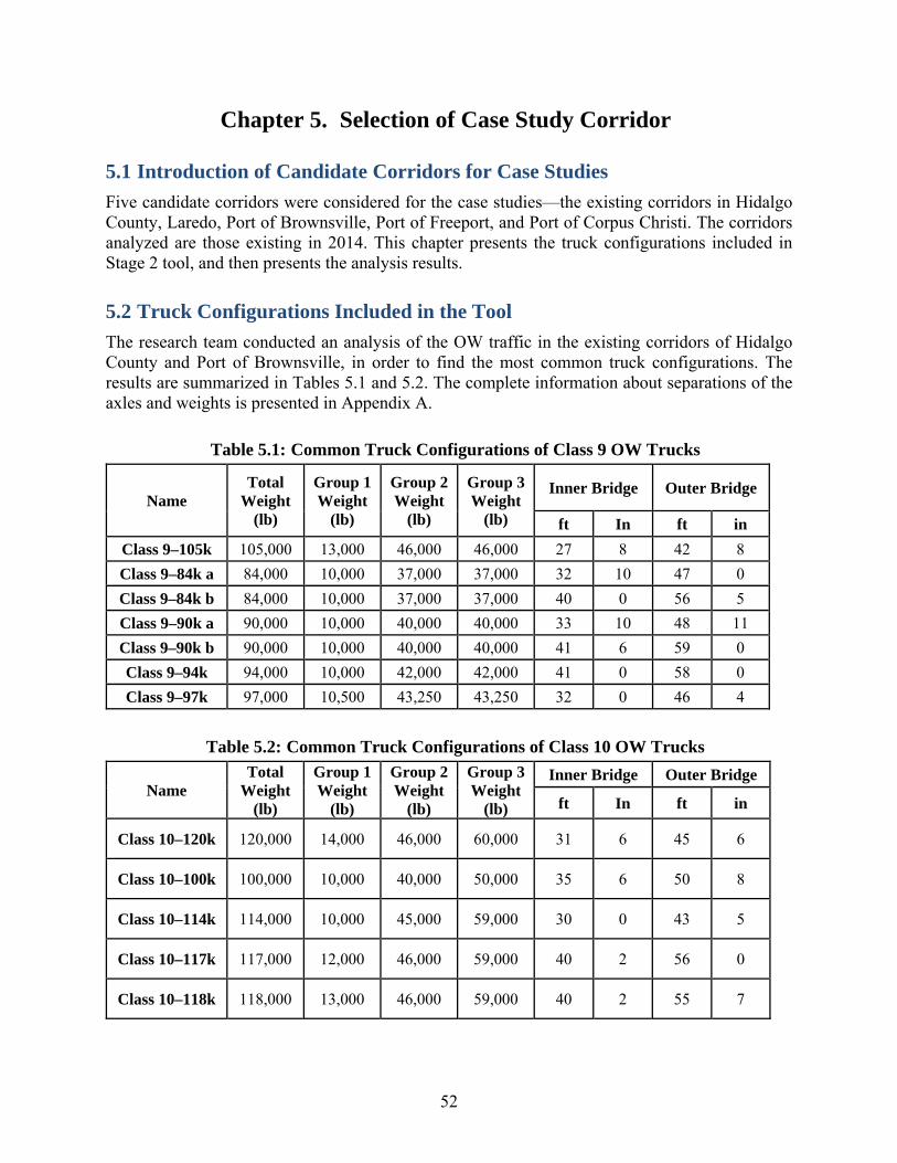
52

Chapter 5. Selection of Case Study Corridor

5.1 Introduction of Candidate Corridors for Case Studies

Five candidate corridors were considered for the case studies—the existing corridors in Hidalgo County, Laredo, Port of Brownsville, Port of Freeport, and Port of Corpus Christi. The corridors analyzed are those existing in 2014. This chapter presents the truck configurations included in Stage 2 tool, and then presents the analysis results.

5.2 Truck Configurations Included in the Tool

The research team conducted an analysis of the OW traffic in the existing corridors of Hidalgo County and Port of Brownsville, in order to find the most common truck configurations. The results are summarized in Tables 5.1 and 5.2. The complete information about separations of the axles and weights is presented in Appendix A.

Table 5.1: Common Truck Configurations of Class 9 OW Trucks

Name Total

Weight (lb)

Group 1 Weight

(lb)

Group 2 Weight

(lb)

Group 3 Weight

(lb)

Inner Bridge Outer Bridge

ft In ft in

Class 9–105k 105,000 13,000 46,000 46,000 27 8 42 8

Class 9–84k a 84,000 10,000 37,000 37,000 32 10 47 0

Class 9–84k b 84,000 10,000 37,000 37,000 40 0 56 5

Class 9–90k a 90,000 10,000 40,000 40,000 33 10 48 11

Class 9–90k b 90,000 10,000 40,000 40,000 41 6 59 0

Class 9–94k 94,000 10,000 42,000 42,000 41 0 58 0

Class 9–97k 97,000 10,500 43,250 43,250 32 0 46 4

Table 5.2: Common Truck Configurations of Class 10 OW Trucks

Name Total

Weight (lb)

Group 1 Weight

(lb)

Group 2 Weight

(lb)

Group 3 Weight

(lb)

Inner Bridge Outer Bridge

ft In ft in

Class 10–120k 120,000 14,000 46,000 60,000 31 6 45 6

Class 10–100k 100,000 10,000 40,000 50,000 35 6 50 8

Class 10–114k 114,000 10,000 45,000 59,000 30 0 43 5

Class 10–117k 117,000 12,000 46,000 59,000 40 2 56 0

Class 10–118k 118,000 13,000 46,000 59,000 40 2 55 7

53

In general, OW trucks in Hidalgo County tend to be longer than trucks in the Port of Brownsville area. Following are the most common configurations in the Port of Brownsville:

• Class 9 – 105k • Class 9 – 84k a • Class 9 – 90k a • Class 9 – 97k • Class 10 – 120k • Class 10 – 100k • Class 10 – 114k

On the other hand, the most common configurations in Hidalgo County are: • Class 9 – 105k • Class 9 – 84k b • Class 9 – 90k b • Class 9 – 94k • Class 10 – 120k • Class 10 – 117k • Class 10 – 118k

5.3 Analysis Results

For the existing corridors, the estimated permit costs are shown in Table 5.3. Detailed information about the analysis is presented in Appendix C.

Table 5.3: Estimated Permit Costs of Existing Corridors

Corridor Permit Cost

HCRMA Existing Corridor 2014 $50.42

Laredo Existing Corridor 2014 $10.82

Port of Brownsville Existing Corridor 2014 $29.48

Port of Freeport Existing Corridor 2014 $25.03

Port of Corpus Christi Existing Corridor 2014 $27.24

54

Chapter 6. Workshop Summary

The research team hosted a workshop with representatives from ports, RMAs, and the trucking industry the morning of April 29, 2016, at the Center for Transportation Research. During this first workshop, the team introduced the meeting objectives, explained the pavement and bridge consumption analysis, presented findings about permits for current corridors and field survey results, demonstrated the analysis tool, and discussed some issues. Another workshop was held that afternoon in the same conference room. Title “Container and Chassis 101,” this second workshop was a presented in conjunction with an industry representative to explore topics related to container shipments.

55

Appendix A. Separations of the Axles and Weights of Each Truck Configuration

Figure A.1. Class 9-84K a

Figure A.2. Class 9-84K b

Figure A.3. Class 9-90K a

56

Figure A.4. Class 9-90K b

Figure A.5. Class 9-94K

Figure A.6. Class 9-97K

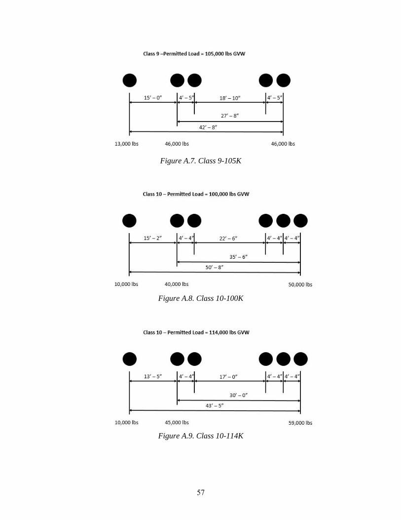
57

Figure A.7. Class 9-105K

Figure A.8. Class 10-100K

Figure A.9. Class 10-114K

58

Figure A.10. Class 10-117K

Figure A.11. Class 10-118K

Figure A.12. Class 10-120K

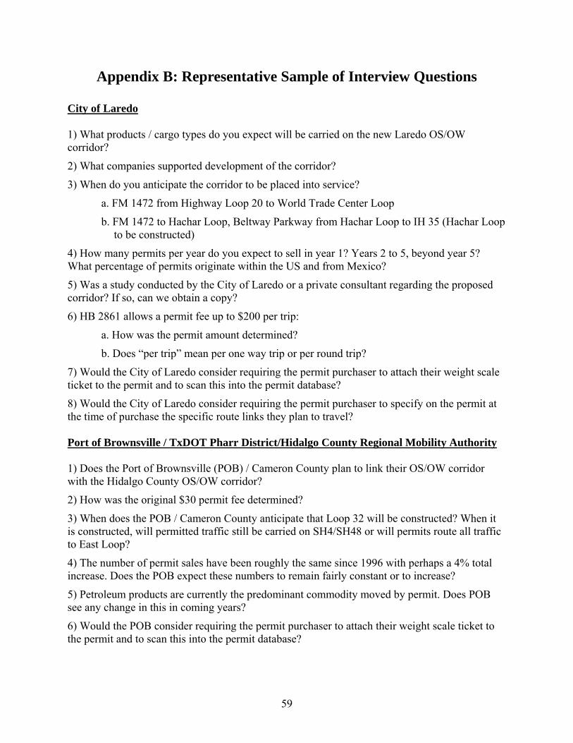
59

Appendix B: Representative Sample of Interview Questions

City of Laredo

1) What products / cargo types do you expect will be carried on the new Laredo OS/OW corridor?

2) What companies supported development of the corridor?

3) When do you anticipate the corridor to be placed into service?

a. FM 1472 from Highway Loop 20 to World Trade Center Loop

b. FM 1472 to Hachar Loop, Beltway Parkway from Hachar Loop to IH 35 (Hachar Loop to be constructed)

4) How many permits per year do you expect to sell in year 1? Years 2 to 5, beyond year 5? What percentage of permits originate within the US and from Mexico?

5) Was a study conducted by the City of Laredo or a private consultant regarding the proposed corridor? If so, can we obtain a copy?

6) HB 2861 allows a permit fee up to $200 per trip:

a. How was the permit amount determined?

b. Does “per trip” mean per one way trip or per round trip?

7) Would the City of Laredo consider requiring the permit purchaser to attach their weight scale ticket to the permit and to scan this into the permit database?

8) Would the City of Laredo consider requiring the permit purchaser to specify on the permit at the time of purchase the specific route links they plan to travel? Port of Brownsville / TxDOT Pharr District/Hidalgo County Regional Mobility Authority 1) Does the Port of Brownsville (POB) / Cameron County plan to link their OS/OW corridor with the Hidalgo County OS/OW corridor?

2) How was the original $30 permit fee determined?

3) When does the POB / Cameron County anticipate that Loop 32 will be constructed? When it is constructed, will permitted traffic still be carried on SH4/SH48 or will permits route all traffic to East Loop?

4) The number of permit sales have been roughly the same since 1996 with perhaps a 4% total increase. Does the POB expect these numbers to remain fairly constant or to increase?

5) Petroleum products are currently the predominant commodity moved by permit. Does POB see any change in this in coming years?

6) Would the POB consider requiring the permit purchaser to attach their weight scale ticket to the permit and to scan this into the permit database?

60

7) Would the POB consider requiring the permit purchaser to specify on the permit at the time of purchase the specific route links they plan to travel?

61

Appendix C. Detailed Information about the Case Study

HCRMA Existing Corridor as of 2014

Description of Hidalgo County RMA’s Existing Corridor As shown in Figure C.1, there are 11 routes in the HCRMA corridor: UP 0281, SH 0336, FM 1016, FM 0396, FM 2061, US 0281, FM 2257, FM 1015, SS 0600, SS 0029, FM 3072 and FM 1472. The total length of the corridor is 54 miles. There are 10,500 OW trucks going through this corridor annually.

Figure C.1 Map of HCRMA (Existing Corridor in 2014)

Attributes of Each Route and Segment

Route 1: UP 0281

The functional class of this route is US. The total length of the route is 3.1 miles. This route is in a rural area in Hidalgo County. The route has one segment, which is described below: Segment 1:

• Physical Boundaries: this segment starts from intersection with Pharr-Reynosa International Bridge and ends at intersection with SH0336.

• Segment Length: This segment has a length of 3.1 miles with two lanes in total. • Pavement Type: The pavement type of this segment is ACP. • Truck Configuration Distribution:

o Configuration 1 (Class 9 105k): 25%

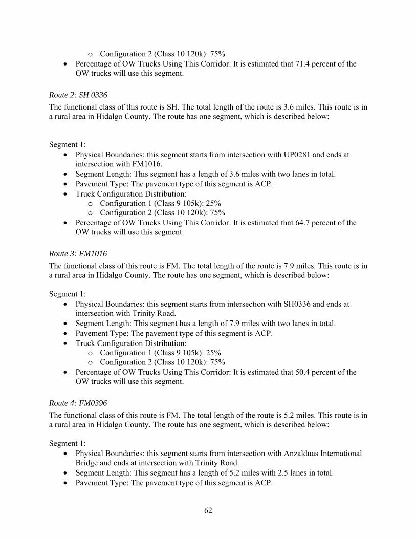
62

o Configuration 2 (Class 10 120k): 75% • Percentage of OW Trucks Using This Corridor: It is estimated that 71.4 percent of the

OW trucks will use this segment.

Route 2: SH 0336

The functional class of this route is SH. The total length of the route is 3.6 miles. This route is in a rural area in Hidalgo County. The route has one segment, which is described below: Segment 1:

• Physical Boundaries: this segment starts from intersection with UP0281 and ends at intersection with FM1016.

• Segment Length: This segment has a length of 3.6 miles with two lanes in total. • Pavement Type: The pavement type of this segment is ACP. • Truck Configuration Distribution:

o Configuration 1 (Class 9 105k): 25% o Configuration 2 (Class 10 120k): 75%

• Percentage of OW Trucks Using This Corridor: It is estimated that 64.7 percent of the OW trucks will use this segment.

Route 3: FM1016

The functional class of this route is FM. The total length of the route is 7.9 miles. This route is in a rural area in Hidalgo County. The route has one segment, which is described below: Segment 1:

• Physical Boundaries: this segment starts from intersection with SH0336 and ends at intersection with Trinity Road.

• Segment Length: This segment has a length of 7.9 miles with two lanes in total. • Pavement Type: The pavement type of this segment is ACP. • Truck Configuration Distribution:

o Configuration 1 (Class 9 105k): 25% o Configuration 2 (Class 10 120k): 75%

• Percentage of OW Trucks Using This Corridor: It is estimated that 50.4 percent of the OW trucks will use this segment.

Route 4: FM0396

The functional class of this route is FM. The total length of the route is 5.2 miles. This route is in a rural area in Hidalgo County. The route has one segment, which is described below: Segment 1:

• Physical Boundaries: this segment starts from intersection with Anzalduas International Bridge and ends at intersection with Trinity Road.

• Segment Length: This segment has a length of 5.2 miles with 2.5 lanes in total. • Pavement Type: The pavement type of this segment is ACP.

63

• Truck Configuration Distribution: o Configuration 1 (Class 9 105k): 25% o Configuration 2 (Class 10 120k): 75%

• Percentage of OW Trucks Using This Corridor: It is estimated that 6.7 percent of the OW trucks will use this segment.

Route 5: FM2061

The functional class of this route is FM. The total length of the route is 2 miles. This route is in a rural area in Hidalgo County. The route has one segment, which is described below: Segment 1:

• Physical Boundaries: this segment starts from intersection with FM3072 and ends at intersection with UP0281.

• Segment Length: This segment has a length of 2 miles with two lanes in total. • Pavement Type: The pavement type of this segment is ACP. • Truck Configuration Distribution:

o Configuration 1 (Class 9 105k): 25% o Configuration 2 (Class 10 120k): 75%

• Percentage of OW Trucks Using This Corridor: It is estimated that 6.7 percent of the OW trucks will use this segment.

Route 6: FM2061

The functional class of this route is FM. The total length of the route is 16.3 miles. This route is in a rural area in Hidalgo County. The route starts from Intersection with Pharr-Reynosa International Bridge (SS0600) and ends at FM1015. The route has three segments, which are described below: Segment 1:

• Physical Boundaries: this segment starts from intersection with Pharr-Reynosa International Bridge (SS0600) and ends at intersection with Spur 29.

• Segment Length: This segment has a length of 1 mile with one lane in total. • Pavement Type: The pavement type of this segment is ACP. • Truck Configuration Distribution:

o Configuration 1 (Class 9 105k): 25% o Configuration 2 (Class 10 120k): 75%

• Percentage of OW Trucks Using This Corridor: It is estimated that 23.8 percent of the OW trucks will use this segment.

Segment 2:

• Physical Boundaries: this segment starts from intersection with Pharr-Reynosa International Bridge (SS0600) and ends at intersection with Anaya Road.

• Segment Length: This segment has a length of 1 mile with two lanes in total. • Pavement Type: The pavement type of this segment is ACP. • Truck Configuration Distribution:

o Configuration 1 (Class 9 105k): 25%

64

o Configuration 2 (Class 10 120k): 75% • Percentage of OW Trucks Using This Corridor: It is estimated that 6.7 percent of the

OW trucks will use this segment.

Segment 3: • Physical Boundaries: this segment starts from intersection with Spur 29 and ends at

intersection with FM1015. • Segment Length: This segment has a length of 14.3 miles with one lane in total. • Pavement Type: The pavement type of this segment is ACP. • Truck Configuration Distribution:

o Configuration 1 (Class 9 105k): 25% o Configuration 2 (Class 10 120k): 75%

• Percentage of OW Trucks Using This Corridor: It is estimated that 6.7 percent of the OW trucks will use this segment.

Route 7: FM2257

The functional class of this route is FM. The total length of the route is 7.4 miles. This route is in a rural area in Hidalgo County. The route has one segment, which is described below: Segment 1:

• Physical Boundaries: this segment starts from intersection with US0281 and ends at intersection with IH0002 (US0083).

• Segment Length: This segment has a length of 7.4 miles with one lane in total. • Pavement Type: The pavement type of this segment is ACP. • Truck Configuration Distribution:

o Configuration 1 (Class 9 105k): 25% o Configuration 2 (Class 10 120k): 75%

• Percentage of OW Trucks Using This Corridor: It is estimated that 14.2 percent of the OW trucks will use this segment.

Route 8: FM1015

The functional class of this route is FM. The total length of the route is 3.2 miles. This route is in a rural area in Hidalgo County. The route has one segment, which is described below: Segment 1:

• Physical Boundaries: this segment starts from intersection with US0281 and ends at intersection with Progresso International Bridge.

• Segment Length: This segment has a length of 3.2 miles with two lanes in total. • Pavement Type: The pavement type of this segment is ACP. • Truck Configuration Distribution:

o Configuration 1 (Class 9 105k): 25% o Configuration 2 (Class 10 120k): 75%

• Percentage of OW Trucks Using This Corridor: It is estimated that 6.7 percent of the OW trucks will use this segment.

65

Route 9: SS0600

The functional class of this route is SS. The total length of the route is 1.9 miles. This route is in a rural area in Hidalgo County. The route has one segment, which is described below: Segment 1:

• Physical Boundaries: this segment starts from Pharr-Reynosa International Bridge and ends at intersection with US0281.

• Segment Length: This segment has a length of 1.9 miles with two lanes in total. • Pavement Type: The pavement type of this segment is ACP. • Truck Configuration Distribution:

o Configuration 1 (Class 9 105k): 25% o Configuration 2 (Class 10 120k): 75%

• Percentage of OW Trucks Using This Corridor: It is estimated that 100 percent of the OW trucks will use this segment.

Route 10: SS0029

The functional class of this route is SS. The total length of the route is 0.3 miles. This route is in a rural area in Hidalgo County. The route has one segment, which is described below: Segment 1:

• Physical Boundaries: this segment starts from intersection with US0281 and ends at intersection with Doffin Canal Road.

• Segment Length: This segment has a length of 0.3 miles with one lane in total. • Pavement Type: The pavement type of this segment is ACP. • Truck Configuration Distribution:

o Configuration 1 (Class 9 105k): 25% o Configuration 2 (Class 10 120k): 75%

• Percentage of OW Trucks Using This Corridor: It is estimated that 6.7 percent of the OW trucks will use this segment.

Route 11: FM3072

The functional class of this route is SS. The total length of the route is 2 miles. This route is in a rural area in Hidalgo County. The route has one segment, which is described below:

Segment 1: • Physical Boundaries: this segment starts from intersection with Veterans Boulevard (“I”

Road) and ends at intersection with Cesar Chavez Road. • Segment Length: This segment has a length of 2 miles with one lane in total. • Pavement Type: The pavement type of this segment is ACP. • Truck Configuration Distribution:

o Configuration 1 (Class 9 105k): 25% o Configuration 2 (Class 10 120k): 75%

• Percentage of OW Trucks Using This Corridor: It is estimated that 11.9 percent of the OW trucks will use this segment.

66

Laredo Existing Corridor as of 2014

Description of Laredo’s Existing Corridor As shown in Figure C.2, there is only one route in the Laredo corridor: FM1472. This route has a length of 4.6 miles. There are 1000 OW trucks going through this corridor annually.

Figure C.2 Map of Laredo (Existing Corridor 2014)

Attributes of Each Route and Segment

Route 1: FM1472

The functional class of this route is FM. The total length of the route is 4.6 miles. This route is in an urban area in Webb County. The route has one segment, which is described below: Segment 1:

• Physical Boundaries: this segment starts from intersection with Loop 20 and ends at northern intersection with World Trade Center Loop.

• Segment Length: This segment has a length of 4.6 miles with two lanes in total. • Pavement Type: The pavement type of this segment is ACP. • Truck Configuration Distribution:

o Configuration 1 (Class 9 105k): 33% o Configuration 2 (Class 10 120k): 67%

• Percentage of OW Trucks Using This Corridor: It is estimated that 100 percent of the OW trucks will use this segment.

67

Port of Brownsville Existing Corridor as of 2014

Description of Port of Brownsville’s Existing Corridor As shown in Figure C.3, there are four routes in the Port of Brownsville corridor: FM511, SH4, SH48, and US77. The total length of this corridor is 19 miles. There are 30,000 OW trucks going through this corridor.

Figure C.3 Map of Port of Brownsville (Existing Corridor 2014)

Attributes of Each Route and Segment

Route 1: FM511

The functional class of this route is FM. The total length of the route is 1.5 miles. This route starts from intersection with SH0048 and ends at Port of Brownsville. This route is in an urban area of Cameron County. The route has two segments: Segment 1:

• Physical Boundaries: this segment starts from intersection with SH0048. • Segment Length: This segment has a length of 1 mile with two lanes in total.

68

• Pavement Type: The pavement type of this segment is ACP. • Truck Configuration Distribution:

o Configuration 1 (Class 9 105k): 33% o Configuration 2 (Class 10 120k): 67%

• Percentage of OW Trucks Using This Corridor: It is estimated that 100 percent of the OW trucks will use this segment.

Segment 2: • Physical Boundaries: this segment ends at Port of Brownsville. • Segment Length: This segment has a length of 0.5 mile with two lanes in total. • Pavement Type: The pavement type of this segment is ACP. • Truck Configuration Distribution:

o Configuration 1 (Class 9 105k): 33% o Configuration 2 (Class 10 120k): 67%

• Percentage of OW Trucks Using This Corridor: It is estimated that 100 percent of the OW trucks will use this segment.

Route 2: SH4

The functional class of this route is SH. The total length of the route is 2.4 miles. This route is in Cameron county and in urban area. The route has two segments: Segment 1:

• Segment Length: This segment has a length of 2.3 miles with two lanes in total. • Pavement Type: The pavement type of this segment is ACP. • Truck Configuration Distribution:

o Configuration 1 (Class 9 105k): 33% o Configuration 2 (Class 10 120k): 67%

• Percentage of OW Trucks Using This Corridor: It is estimated that 100 percent of the OW trucks will use this segment.

Segment 2: • Segment Length: This segment has a length of 0.1 miles with two lanes in total. • Pavement Type: The pavement type of this segment is JCP. • Truck Configuration Distribution:

o Configuration 1 (Class 9 105k): 33% o Configuration 2 (Class 10 120k): 67%

• Percentage of OW Trucks Using This Corridor: It is estimated that 100 percent of the OW trucks will use this segment.

Route 3: SH48

The functional class of this route is SH. The total length of the route is 4.3 miles. This route starts from intersection with SH0004 and ends at intersection with FM0511. This route is in an urban area of Cameron County. The route has four segments: Segment 1:

69

• Physical Boundaries: this segment starts from intersection with SH0005. • Segment Length: This segment has a length of 0.5 mile with three lanes in total. • Pavement Type: The pavement type of this segment is ACP. • Truck Configuration Distribution:

o Configuration 1 (Class 9 105k): 33% o Configuration 2 (Class 10 120k): 67%

• Percentage of OW Trucks Using This Corridor: It is estimated that 100 percent of the OW trucks will use this segment.

Segment 2: • Segment Length: This segment has a length of 2.4 mile with two lanes in total. • Pavement Type: The pavement type of this segment is ACP. • Truck Configuration Distribution:

o Configuration 1 (Class 9 105k): 33% o Configuration 2 (Class 10 120k): 67%

• Percentage of OW Trucks Using This Corridor: It is estimated that 100 percent of the OW trucks will use this segment.

Segment 3: • Segment Length: This segment has a length of 0.6 mile with two lanes in total. • Pavement Type: The pavement type of this segment is ACP. • Truck Configuration Distribution:

o Configuration 1 (Class 9 105k): 33% o Configuration 2 (Class 10 120k): 67%

• Percentage of OW Trucks Using This Corridor: It is estimated that 100 percent of the OW trucks will use this segment.

Segment 4: • Physical Boundaries: this segment starts from intersection with FM0511. • Segment Length: This segment has a length of 0.8 mile with two lanes in total. • Pavement Type: The pavement type of this segment is ACP. • Truck Configuration Distribution:

o Configuration 1 (Class 9 105k): 33% o Configuration 2 (Class 10 120k): 67%

• Percentage of OW Trucks Using This Corridor: It is estimated that 100 percent of the OW trucks will use this segment.

Route 4: US77

The functional class of this route is US. The total length of the route is 2.2 miles. This route is in an urban area of Cameron County. The route has three segments: Segment 1:

• Segment Length: This segment has a length of 1 mile with 2.5 lanes in total. • Pavement Type: The pavement type of this segment is ACP. • Truck Configuration Distribution:

70

o Configuration 1 (Class 9 105k): 33% o Configuration 2 (Class 10 120k): 67%

• Percentage of OW Trucks Using This Corridor: It is estimated that 100 percent of the OW trucks will use this segment.

Segment 2: • Segment Length: This segment has a length of 0.6 mile with three lanes in total. • Pavement Type: The pavement type of this segment is ACP. • Truck Configuration Distribution:

o Configuration 1 (Class 9 105k): 33% o Configuration 2 (Class 10 120k): 67%

• Percentage of OW Trucks Using This Corridor: It is estimated that 100 percent of the OW trucks will use this segment.

Segment 3: • Segment Length: This segment has a length of 0.6 mile with two lanes in total. • Pavement Type: The pavement type of this segment is ACP. • Truck Configuration Distribution:

o Configuration 1 (Class 9 105k): 33% o Configuration 2 (Class 10 120k): 67%

• Percentage of OW Trucks Using This Corridor: It is estimated that 100 percent of the OW trucks will use this segment.

71

Port of Freeport Existing Corridor as of 2014

Description of Port of Freeport’s Existing Corridor As shown in Figure C.4, there are five routes in Port of Freeport’s existing corridor: FM0523, FM1495, SH0288, SH0036, and SH0332. The total length of this corridor is 24 miles. There are 250 OW trucks going through this corridor.

Figure C.4 Map of Port of Freeport (Existing Corridor 2014)

72

Attributes of Each Route and Segment

Route 1: FM0523

The functional class of this route is FM. The total length of the route is 7.1 miles. This route is in an urban area of Brazoria County. The route has one segment: Segment 1:

• Physical Boundaries: this segment starts from intersection with Moller Road (FM0226) and ends at intersection with FM1495.

• Segment Length: This segment has a length of 7.1 miles with one lane in total. • Pavement Type: The pavement type of this segment is ACP. • Truck Configuration Distribution:

o Configuration 1 (Class 9 105k): 33% o Configuration 2 (Class 10 120k): 67%

• Percentage of OW Trucks Using This Corridor: It is estimated that 29 percent of the OW trucks will use this segment.

Route 2: FM1495

The functional class of this route is FM. The total length of the route is 4.9 miles. This route is in an urban area of Brazoria County. The route has one segment: Segment 1:

• Physical Boundaries: this segment starts from intersection with FM0523 and ends at intersection with SH0036.

• Segment Length: This segment has a length of 4.9 miles with one lane in total. • Pavement Type: The pavement type of this segment is ACP. • Truck Configuration Distribution:

o Configuration 1 (Class 9 105k): 33% o Configuration 2 (Class 10 120k): 67%

• Percentage of OW Trucks Using This Corridor: It is estimated that 29 percent of the OW trucks will use this segment.

Route 3: SH0288

The functional class of this route is SH. The total length of the route is 7.4 miles. This route is in an urban area of Brazoria County. The route has one segment: Segment 1:

• Physical Boundaries: this segment starts from intersection with Sycamore Street (also named Chlorine Road) and ends at intersection with SH0036.

• Segment Length: This segment has a length of 7.4 miles with three lanes in total. • Pavement Type: The pavement type of this segment is CRCP. • Truck Configuration Distribution:

o Configuration 1 (Class 9 105k): 33% o Configuration 2 (Class 10 120k): 67%

73

• Percentage of OW Trucks Using This Corridor: It is estimated that 71 percent of the OW trucks will use this segment.

Route 4: SH0036

The functional class of this route is SH. The total length of the route is 1.3 miles. This route is in an urban area of Brazoria County. The route has one segment: Segment 1:

• Physical Boundaries: this segment starts from intersection with SH0288 and ends at intersection with FM1495.

• Segment Length: This segment has a length of 1.3 miles with one lane in total. • Pavement Type: The pavement type of this segment is ACP. • Truck Configuration Distribution:

o Configuration 1 (Class 9 105k): 33% o Configuration 2 (Class 10 120k): 67%

• Percentage of OW Trucks Using This Corridor: It is estimated that 71 percent of the OW trucks will use this segment.

Route 5: SH0332

The functional class of this route is SH. The total length of the route is 3.7 miles. This route is in an urban area of Brazoria County. The route has one segment: Segment 1:

• Physical Boundaries: this segment starts from intersection with SH0288 and ends at intersection with FM0523.

• Segment Length: This segment has a length of 3.7 miles with one lane in total. • Pavement Type: The pavement type of this segment is CRCP. • Truck Configuration Distribution:

o Configuration 1 (Class 9 105k): 33% o Configuration 2 (Class 10 120k): 67%

• Percentage of OW Trucks Using This Corridor: It is estimated that 15 percent of the OW trucks will use this segment.

74

Port of Corpus Christi Existing Corridor as of 2014

Description of Port of Corpus Christi’s Existing Corridor As shown in Figure C.5, there are three routes in the Port of Corpus Christi’s corridor: US01841, SH0035, and SH0361. The total length of this corridor is 26 miles. There are 1000 OW trucks going through this corridor.

Figure C.5 Map of Port of Corpus Christi (Existing Corridor 2014)

Attributes of Each Route and Segment

Route 1: US0181

The functional class of this route is US. The total length of the route is 13.3 miles. This route is in an urban area of San Patricio County. The route has two segments: Segment 1:

• Physical Boundaries: this segment starts from intersection with Burleson Street and ends at intersection with SH0035.

• Segment Length: This segment has a length of 8.7 miles with two lanes in total. • Pavement Type: The pavement type of this segment is ACP. • Truck Configuration Distribution:

o Configuration 1 (Class 9 105k): 33%

75

o Configuration 2 (Class 10 120k): 67% • Percentage of OW Trucks Using This Corridor: It is estimated that 38 percent of the OW

trucks will use this segment.

Segment 2: • Physical Boundaries: this segment starts from intersection with SH0035 and ends at

intersection with County Road 3567 (Midway Road). • Segment Length: This segment has a length of 4.6 miles with two lanes in total. • Pavement Type: The pavement type of this segment is ACP. • Truck Configuration Distribution:

o Configuration 1 (Class 9 105k): 33% o Configuration 2 (Class 10 120k): 67%

• Percentage of OW Trucks Using This Corridor: It is estimated that 100 percent of the OW trucks will use this segment.

Route 1: SH0035

The functional class of this route is FM. The total length of the route is 5.7 miles. This route is in an urban area of San Patricio County. The route has one segment: Segment 1:

• Physical Boundaries: this segment starts from intersection with US0181 and ends at intersection with FM3512.

• Segment Length: This segment has a length of 4.6 miles with two lanes in total. • Pavement Type: The pavement type of this segment is ACP. • Truck Configuration Distribution:

o Configuration 1 (Class 9 105k): 33% o Configuration 2 (Class 10 120k): 67%

• Percentage of OW Trucks Using This Corridor: It is estimated that 36 percent of the OW trucks will use this segment.

Route 2: SH0361

The functional class of this route is SH. The total length of the route is 6 miles. This route is in an urban area of San Patricio County. The route has one segment: Segment 1:

• Physical Boundaries: this segment starts from intersection with SH0035 and ends at intersection with FM1069 (Main Street).

• Segment Length: This segment has a length of 6 miles with two lanes in total. • Pavement Type: The pavement type of this segment is ACP. • Truck Configuration Distribution:

o Configuration 1 (Class 9 105k): 33% o Configuration 2 (Class 10 120k): 67%

• Percentage of OW Trucks Using This Corridor: It is estimated that 27 percent of the OW trucks will use this segment.