I '~~~ADA1387-

Technical Report 837

TRIDENT BIOLOGICAL SURVEYS: N.AVALSSUBMARINE BASE BANGOR, WASHINGTON

"(1979, 1980 & 1981) SUMMARY REPORT(SUPPLEMENT 3 TO NUC TP 510)

J. G. Grovhoug

15 September 1982

Prepared forNaval Submarine Base

Bangor, Washington

Approved for public release; distribution unlimited

DTICJAN 2 7 1983

SB .. NAVAL OCEAN SYSTEMS CENTER- San Diego, California 92152

83 01 27 009

a

NAVAL OCEAN SYSTEMS CENTER, SAN DIEGO, CA 92152

AN ACTIVITY OF THE NAVAL MATERIAL COMMAND

JM PATTON, CAPT, USN HIL BLOODCommander Techincal Director

ADMINISTRATIVE INFORMATION

This task was performed by members of the Marine Sciences Division (Code 513) of

the Naval Ocean Systems Center. Specific site surveys were performed during 6-16 Jun 79,

23 Jun - 3 Jul 80 and 27 May - 11 Jun 81., These efforts were supported by funds adminis-

tered by the Naval Facilities Engineering Command through the Officer in Charge of Con-

struction, Trident, under work request numbers N68248-79-WR-00047, N68248-80-WR-

00026 and Naval Submarine Base, Bangor work request number N68436-81-WR-20004.

The author thanks the following individuals for their contributions to various aspects

of this report: T.J. Peeling, H.W. Goforth, J.H, Reeves, D.E. Morris, R.L. Carter, R.B. Roholt,

R.A. Dietz and W.J. Cooke for on-site support, field collections and data recording; R.A.Dietz, W.J. Cooke and R.L. Fransham for data reduction and processing; P.F. Seligman and

R.L. Chambers for heavy metal analyses; W.A. Friedl and S.A. Patterson for their carefulreview of the manuscript for this report; D. Colburn and M. Guidry for their outstandingskills with graphics and technical illustration; and R.H. Brady for his detailed editing andassistance wit1n publications procedures.

Released by Under authority ofRR SOULE, Head HO PORTER, HeadMarine Sciences Division Biosciences Department

V

SECURITY CLAWS1CATION OF THIS PAGE (When Datd _ _ __O_.

READ flSTRUCTIOISREPORT DO•ICENTATION PAGE BEFORE COMPLEsTIN FORM

0. N1 1 7U M .lG O V Tr A C C E S S IO N N O W. R E C P I E NT S C A T A L O G N U M IE R

NOSC Technical Report 837 (TR 837) 31I4. TITLE (And Subdtie) S. TYPE OF REPORT & PERIOD COVERED

TRIDENT BIOLWGICAL SURVEYS: NAVAL SUBMARINE BASEBANGOR, WASHINGTON (1979,1980 & 1981) SUMMARY REPORT _INl.________,__,_____"

(SUPPLEMENT 3 TO NUC TP 510) S. PERFORMING ORG. REPORT NUMUER

7. AUTHOR(e) S. CONTRACT OR GRANT NUMIER(t)

Jost,-h G. Grovhoug

9. PERFORMING ORGANIZATION NAME AND ADDRESS 10. PROGRAM ELEMENT. PROJECT, TASK

Naval Ocean Systems Center, Hawaii Laboratory AREA 6 WORK UNIT NUMBIERS

P. 0. Box 997 OMN-NSB-0-513-ME07Kallua, Hawaii 96734

i1. CONTROLLING OFFICE NAME AND ADDRESS 12. REPORT DATE

Naval Submarine Base Bangor, Code 222 15 Sep 82Bremerton, WA 98315 Is. NUMBER OF PAGES

13014. MONITORING AGENCY NAME & ADDRESS(II 4iflfemt from Catoioffbi Office) 1S. SECURITY CLASS. (of 0heat)

Unclassified

15. DECL ASSI FICATIO*/ DOWNGRADINGSCHEDULE

16. DISTRIBUTION tTATEMENT (of Mde RPort)

Approved for public release; distribution unlimited.

17. DISTR1IUTION STATEMENT (of the abetted uttered in Block 20. if diffmst k por)

IS. SUPPLEMENTARY NOTES

It. KEY WORDS (Contnuse an roer"re olds if aeoeeal and idstifp by Mlock m=ber)Biological survey /im, Hood Canal, WA Puget Sound, WABivalve molluscs Marine environmental studies SUBASE BangorFishes 5 ,•,, •M. Nav envirnmental studies Trident submarine baseHeavy metals 1.Nearhore environmentsIntertidal Ecology Oysters.

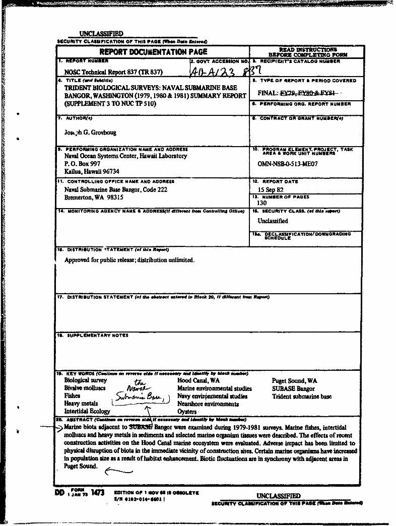
M0 ABSTRACT (Contame do seowe efd.~if -eeeary aid Idineia AV Meek ftwr),>Marine blota adjacent to S Bangor were examined during 1979-1981 surveys. Marine fishes, intertidal

molluscs and heavy metals in sediments and selected marine organism tissues were described. The effects of reetconstruction activities on the Hood Canal marine ecosystem were evaluated. Adverse impact has been limited tophysical disruption of biota in the immediate vicinity of construction sires. Certain marine oq nism have increadin population size as a result of habitat enhancement. Biotic fluctuations are in synchrony with adjacent areas inPuget Sound.

IIFORM I3 EDITION O

JAN 7E O. Io V . BoI..ET UNCLASSIFIED

SEUIYCLASV"1FICA1M ýOP TRS FPAME (Isa4a 1

OBJECTIVES

1. Document annual abundanre- and distribution of commercially and recreationallyimportant marine biota adjacent to SUBASE Bangor.

2. Monitor heavy metal levels in sediments and selected organisms.

3. Provide data to assist SUBASE Bangor resource management planning.

4. Evaluate significant patterns in data collected and compare with previous SUBASEBangor marine environmental survey findings.

5. Recommend future study needs.

RESULTS

1. Habitat for many fish species has increased since 1975.,

2. Marine fish surveys documented diverse nearshore assemblages.

3. Otter trawl sampling for marine fishes was most efficient at night.

4. Feeding habits for selected fish species were described.

5. External parasitic infestation of certain flatfish species was observed,

6. Intertidal bivalve surveys documented the. dernsity and distribution of commercialspecies at seven locations along Hood Canal.

7. Maximum bivalve densities occurred at southern SUBASE Bangor stations.

8. Butter clams yielded the greatest biomass when compared with other intertidalmolluscan biota.

9. Native littleneck clams were the most numerically abundant bivalve species.

10. Extensive oyster beds were observed and described along SUBASE Bangor water-front areas.

11. Heavy metal surveys of selected sediments and tissues were performed in 1980and 198 1.

12. Heavy metal data reflect values similar to other Puget Sound regions.

13. Comparisons were made with earlier SUBASE Bangor marine survey data.

J I

RECOMMENDATIONS

1. Continue to monitor nearshore marine environmental rt~gions annually atSUBASE Bangor.

2. Retain marine fish surveys, intertidal surveys and heavy metal surveys duringfuture monitoring investigations.

3. Develop detailed resource management plans for selected marine biota inhabitingSUBASE Bangor waterfront regions.

4. Document significant ecological events as they occur throughout the year to en-hance annual survey perspectives and evaluations.

5. Encourage selected commercial and recreational utilization of intertidal bivalvesand marine fishes along SUBASE Bangor.

Acoession For

NTIS GRA&IDTIC TkB 0Unannounced 0]JustifiC t•t•

'By-Distribution/Availability Codes

vail and/or

[Dt Special

2

CONTENTS

EXECUTIVE BRIEF... page 7INTRODUCTION ... 9MARINE FISH SURVEYS... 15

Introduction... 15Materials and Methods...: 17Results and Discussion.. 18

Feeding Habits. 22Conclusions .-. ,, 27

INTERTIDAL SURVEYS... Z8Introduction... 28

Bivalve Molluscs... 28Materials and Methods,_. 29Results and Discussion. .,. 34Conclusions... 61

HEAVY METAL SURVEYS.. - 66Introduction .,. 66Materials and Methods .... 67Results and Discussion... 70

Overview ,,., 79Conclusions-.. 83

REFERENCES.,. 84APPENDICES

A. SUBASE Bangor Sampling Stations .:.. 89B. Fish Trawl Catch Data,.. 95C., Oyster Management Plan..., 103D. Bivalve Mollusc Length-Frequency Distributions,.,. 109E. Selected Important Species... 115F. Taxonomic Checklist Additions-., , 127

ILLUSTRATIONS

1 Hood Canal in perspective to the Pacific Basin. ..,. page 122 Sampling stations and points of reference along SUBASE Banor waterfront areas -. ,., 133 Otter trawl sampling locations adjacent to SUBASE Bangor ., ,.., i 64 Horizontal and vertical distribution of major species of bivalve molluscs along

SUBASE Bangor.... 315 NOSC field team member sighting intertidal transect line position using a hand-held

magnetic bearing compass... 326 Oyster beds along SUBASE Bangor surveyed June-July, 1981. .,. 357 Integrated beach profile: Station A... 368 Integrated beach profile: Station Z ... 379 Integrated beach profile: Station C... 38

10 Integrated beach profile: Station D ... 39

3

ILLUSTRATIONS

11 Integrated beach profile: Station G... 4012. Integrated beach profile: Station J,... 4113 Integrated beach profile: Station M •.. 4214 Sediment sample locations for heavy metal core sample collections,

SUBASE Bangor. .. 6815 Organism collection locations, heavy metals... 69

TABLES

1 Summary of Trident construction activities at SUBASE Bangor duringthe period 1975-1981 . .,., page 14

2 List of Hood Canal fishes collected during Trident environmental monitoringsurveys (1979-1981)... 19

3 Summarized otter trawl data (1979-1981) ... 204 Data summary for nighttime otter trawls conducted at SUBASE Bangor

during 1979, 1980 and 1981 .. , 215 Rock sole infestation by Philometra americana. ,. 236 Flatfish other than rock sole infested by P. americana ... 237 Diet categories for selected fishes collected adjacent to SUBASE Bangor

in Hood Canal during 1979, 1980 and 1981 surveys •. . 248 SUBASE Bangor intertidal station transect parameters during 1979, 1980 and

1981 surveys.. . 309 Intertidal bivalve species frequency: Station A. ,.. 43

10 Intertidal bivalve species frequency: Station Z.... 4411 Intertidal bivalve species frequency: Station C... 4512 Intertidal bivalve species frequency: Station D ,... 4613 Intertidal bivalve species frequency: Station G .. 4714 Intertidal bivalve species frequency: Station J ,.,. 4815 Intertidal bivalve species frequency: Station M ... 4816 Combined mean intertidal bivalve density (#/m2) ... 5817 Commercial clam species recruitment (#/m 2 )... 5918 Commercial bivalve density (#/m 2) and biomass (kg/m 2 ) collected at

all SUBASE Bangor sampling stations during the period 1976-1981 ... 6010 Commercial dig frequencies at SUBASE Bangor (1979-1981)... 6220 Oyster frequencies (#/m2 ) present in quadrats during intertidal

transect surveys... 6321 Eelgrass bed width, turion density and biomass data collected during

July, 1979 at SUBASE Bangor... 6422 Heavy metal detection limits ,. 71

S23 SUBASE Bangor sediment heavy metal data (1980-1981)... 7124 Rockfish muscle tissue heavy metal data... 7325 Rockfish liver tissue heavy metal data... 7426 Crab muscle tissue heavy metal data... 7527 Crab hepatopancreas tissue heavy metal data. . 7628 Oyster tissue heavy metal data ... 76

4

TABLES

29 Mytilus general tissue heavy metal data (1981 only)... 7730 Mytilus adductor muscle tissue heavy metal data... 7731 Mytilus byssal gland tissue heavy metal data. ,. 7832 Parastichopus californicus muscle tissue heavy metal data (1980 only) ... 8033 A summary of heavy metal content in sediment and tissue samples

collected at SUBASE Bangor (1980-1981)... 8134 Sediment heavy metal data listed in reference 44, for comparison with

SUBASE Bangor data... 8235 Data listed in reference 43, for comparison with SUBASE Bangor data . ... 82

5

EXECUTIVE BRIEF

The marine environment at the Naval Submarine Base, Bangor, Washington was sur-veyed three times between July 1979 and July 1981 in a continuing effort to documentenvironmental conditions along Navy-controlled shoreline areas adjacent to Hood Canal.The surveys provide baseline data for assessments of potential environmental responses tothe newly-constructed Trident Submarine Support Facility. One goal of the surveys is todocument the annual abundance and distribution of commercially and recreationally impor-tant species of marine biota. Another objective is to monitor levels of certain heavy metalsin sediments and in selected marine organisms to provide a yearly measure of trace metalstatus within the-marine community. A third objective is to provide Naval Submarine BaseBangor with meaningful marine environmental data to enhance resource management plan-ning efforts. This summary presents results from refined field surveys made during the com-pletion of major waterfront construction projects along Hood Canal. Only the more reliable,productive and cost-effective field sampling activities from previous surveys were retainedduring the surveys reported here.

Marine fish surveys indicated diverse and apparently healthy assemblages of ichthio-fauna are present along SUBASE Bangor nearshore areas of Hood Canal. Habitat for manyspecies has been greatly enhanced through the addition of waterfront structures. Marine fishcollections during this three-year reporting period totaled more than 2000 specimensrepresenting 37 species from 18 families of fishes. Feeding habit analyses for 17 selectedspecies from 10 families documented 42 categories of diet items. Crustaceans, fishes, poly-chaete worms and bivalve molluscs were the predominant food items for fishes examined.These data indicate that the fish have diverse feeding patterns which are consistent withhealthy, productive marine environmental conditions.

Intertidal surveys showed that commercially and recreationally important bivalvemolluscs are abundant along SUBASE Bangor waterfront areas. These populations experiencenormal fluctuations in recruitment, growth and survival. Maximum densities of commerciallyimportant clams occur two feet on either side of tidal datum (MLLW) along SUBASEBangor. Butter clams represented the highest biomass of important bivalves during thisperiod. Native littleneck clams were the most numerically abundant commercial bivalvespecies. The densest populations of bivalves along SUBASE Bangor were in the southernsampling areas. Harvestable oyster beds now represent a significant resource along SUBASEBangor.

Sediment and tissue heavy metal data are important aspects of continued environ-mental monitoring surveys at SUBASE Bangor. Several species of marine biota sampled at

SUBASE Bangor concentrate certain heavy metals biologically. Heavy metal levels measuredduring 1980 and 1981 indicated levels in sediments and selected biota ate similar at SUBASEBangor stations to other regions of central and southern Puget Sound.

Annual environmental surveys provided consistent and reliable estimates of potentialecosystem response to construction activities during this reporting period. Data from thesesurveys indicate that the marine ecosystem along SUBASE Bangor shoreline has not beenadversely changed by Trident construction activities. Biological fluctuations observed at

*1 ___ ____ 7

SUBASE Bangor are in natural synchrony with fluctuations elsewhere in Hood Canal andother Puget Sound regions. No rare or endangered species or critical marine habitat has beenthreatened by construction activities. Habitat has been effectively enhanced by the increasednumber of piers and wharfs along SUBASE Bangor. Adverse impact has been limited to themarine organisms physically disrupted by the mechanical process of pier construction.

8

INTRODUCTION

In 1973, the Naval Facilities Engineering Command requested that the Naval OceanSystems Center (then designated the Naval Undersea Center) perform a series of biologicalsurveys at the proposed Trident Submarine Support Facility located on Bangor Annex ofthe Keyport Naval Torpedo Station, Washington. This facility has been redesignated NavalSubmarine Base Bangor (SUBASE Bangor). Four seasonal surveys were conducted to pro-vide baseline biological data to assess the effects of construction on commercially and recre-ationally important populations of marine molluscs and fishes. Other marine biota which areimportant components of the Hood Canal ecosystem were sampled to determine their gen-eral condition, abundance and distribution in the study area. Also, a number of improvedenvironmental monitoring techniques were developed and tested during these surveys. Thefirst four surveys - Trident Surveys I-IV - were conducted in June and October 1973, andJanuary and April-May 1974, respectively. A fifth survey was performed in July 1975 at therequest of the officer-in-charge-of-construction for the Trident Facility (OICC Trident). Theresults of surveys I-V were documented in field data reports submitted to OICC Tridentand in reference 1.

In July 1976, a sixth survey (VI) was conducted after waterfront construction beganfor the explosives-handling wharf (EHW) and piling stress testing near the planned DeltaComplex site.. This survey was designed to assess the effects of construction on marine lifeat SUBASE Bangor by comparing new data with those collected during surveys I-V. Theresults of survey V1 were published in reference 2. This report contained an extensive cumu-lative checklist of marine flora and fauna recorded from Hood Canal during surveys I-VI.

In July 1977 and June 1978, surveys VII and VIII, respectively, were conducted tomonitor and evaluate the effects of Trident construction activities on marine life along theSUBASE Bangor waterfront areas. The results of these surveys were analyzed and comparedwith the previous six surveys. A summary report of surveys VII and VIII was published (ref3). Because most shoreline construction was completed before survey VIII, data from thissurvey provided a comparison to evaluate the impact of Trident construction activities onthe marine life at SUBASE Bangor, The data from survey VIII were also used to evaluatefield and analytical methods used during previous surveys to monitor the effects of shore-line construction on resident marine biota. This analysis supported several recommendationsfor improving the survey design and optimizing field collection efforts. Additionally, thisevaluation recommended techniques for effectively monitoring the marine environment atSUBASE Bangor as it is upgraded into an operational Trident submarine training base andrefit facility.

1Naval Undersea Center TP 510, Trident Biological Surveys: A summary report, June 1973 - July 1975,

by TJ Peeling and HW Goforth, 144 p, 19752 Naval Undersea Center TP 510 (Supplement 1), Trident Biological Survey: July 1976, by TJ Peeling,

MH Salazar, JG Grovhoug and HW Goforth, 58p, 19763Naval Ocean Systems Center TR 513 (Supplement 2 to NUC TP 510), Trident Biological Surveys:

SUBASE Bangor (July 1977 and June 1978) and Indian Island Annex (January, May 1974 and June1978), HW Goforth, TJ Peeling, MH Salazar and JG Grovhoug, 84p, 1979

9

Beginning with survey IX in July 1979, several changes in survey design were effected.All sampling locations were critically evaluated in terms of relevant data contribution. Thosesites which were not yielding useful and representative data were deleted.. Some sites wererepositioned and redesignated within the same general region. Intertidal delta regions con-taining major freshets at low tidal periods typically possessed bivalve concentrations muchlower than areas which were qualitatively observable as high-density, productive clammingbeaches. Station E, at Devil's Hole delta, is an example of this pattern. Because we observeddense clam aggregations on either side of the transect area for several years, in 1979 theintertidal sampling station was moved south about 150 metres and redesignated as station D.For the purposes of otter trawl sampling, this station is referred to as station D-E. To thenorth, the problem at station K was similar. Station K was deleted and a new station, desig-nated J, was established about 200 metres north of the old station K. Otter trawl data werelabeled J-K from this area. The new station J, however, was located nearer station L, the off-base northern control site, and thus a new problem was encountered. Station L had consis-tently yielded low-density data for intertidal bivalves and marine fishes. Therefore, in 1979,concurrent with the establishment of station J and based on previous recommendations (ref3), station L was deleted from all further monitoring efforts. Further north, an off-base con-trol station was selected and designated as station M.. This station was sampled intensivelyduring the 1979 survey, but because intertidal bivalve data at this site were not representa-tive of a commercially important station, the utility of station M as an off-base controlstation was questionable. This station was deleted during 1980 and 1981 intertidal bivalvesurveys. However, otter trawl sampling has been retained at station M because representativefish data continue to be collected from this site. The offbase southern control station (A) isconsidered to provide ample representative data for comparison with on-base stations.

Survey X, performed in June-July 1980, included further refinements in SUBASEBangor monitoring survey strategies. Water, sediment and selected organism tissues werecollected and analyzed for selected heavy metals. These data were to be part of a baselinefor monitoring heavy metal conditions along Hood Canal. Results from initial heavy metalanalyses suggested several modifications in monitoring survey design. The data on heavymetals in water had low variability and was generally uninformative; such low variability isexpected from a healthy marine environment. Sediment heavy metal data from some sitessuch as Marginal Wharf and KB Pier had an expected range of values, including typical piersignatures. Future monitoring of sediment heavy metal data at selected waterfront areas wassupported by these data. Heavy metal samples from tissues of rockfish, crabs and musselsyielded data typical for the region., These tissue samples are considered useful for futuremonitoring efforts at SUBASE Bangor.

Additionally, during survey X, nighttime otter trawl collections augmented daytimetrawls to evaluate the effects of time of day on catch. These data indicate that species abun-dance and feeding information are more typical from nighttime hauls.

Survey XI, in May-June 1981, focused on three s,,rveys: marine fish, intertidal andheavy metals. Marine fish and intertidal surveys continue to be central to SUBASE Bangormonitoring efforts. Nighttime otter trawls and intertidal bivalve transects along seven HoodCanal stations yielded representative data during the 1981 survey. The heavy metal surveydesign was modified for future surveys by deleting sea cucumber muscle tissue collectionsand adding oyster tissue samples from selected sites. Sediment samples were collected fromall major waterfront areas which were initially sampled in 1980.

10

The 1981 monitoring survey occurred in late May and early June, during a low tideperiod. Results indicate a reduced abundance and lowered biomass for marine fishes andintertidal bivalves during the early summer of 1981. The reduced catch is chiefly attributableto the earlier sampling period in 1981.• Many juveniles of important sampled species are notgenerally available for sampling until mid-June.

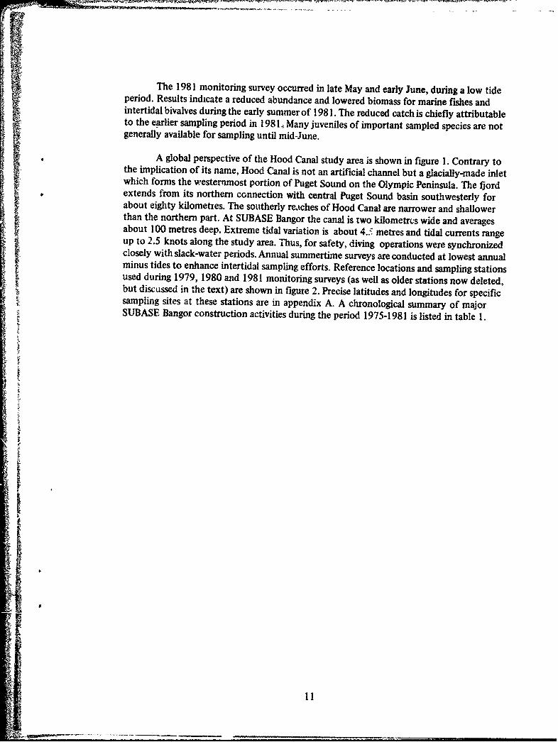
A global perspective of the Hood Canal study area is shown in figure 1. Contrary tothe implication of its name, Hood Canal is not an artificial channel but a glacially-made inletwhich forms the westernmost portion of Puget Sound on the Olympic Peninsula. The fjordextends from its northern connection with central Puget Sound basin southwesterly forabout eighty kilometies. The southerly rea•ches of Hood Canal are narrower and shallowerthan the northern part. At SUBASE Bangor the canal is two kilometrus wide and averagesabout 100 metres deep. Extreme tidal variation is about 4.J metres and tidal currents rangeup to 2.5 knots along the study area. Thus, for safety, diving operations were synchronizedclosely with slack-water periods. Annual summertime surveys are conducted at lowest annualminus tides to enhance intertidal sampling efforts. Reference locations and sampling stationsused during 1979, 1980 and 1981 monitoring surveys (as well as older stations now deleted,but discussed in the text) are shown in figure 2. Precise latitudes and longitudes for specific

4 sampling sites at these stations are in appendix A. A chronological summary of majorSUBASE Bangor construction activities during the period 1975-1981 is listed in table 1.

I

11

2.625 kinm:

Figue 1 Hoo Caal n pespetiveto he acifc Bsin

C1

;X-X-X-:M

:XI

Brw :.. Hoo .. xplosives.

X, NAVAL. ...... .. ...

0 Cope SUMRNBASE-X

1.. Pilemeter....

% xxA

Figure 2.XSampling 'ttosadpitXfrfrneaon UAEBno aefotaes

:-XX__:.%.......... - lo13

WaterfrontYear Structure* Construction Activity

1975 EHW Began const ruction; test pile driving in June.

1976 DC Preliminary pile driving; test wells drilled.

EHW Drove pilings and completed wharf area.

1977 DC Completed pile driving and trestles; dredged entrance channel and drydock area;periodically pumped test wells; started drydock cofferdam construction.

EHW Completed wharf pilings and submarine berth enclosure; lighting partially operationalin May.,

MSF Commenced pile driving.

1978 DC Completed drydock cofferdam and filling activities; drydock area dewatered;completed dredging within drydock.

EHW Completed lighting installation and began operational testing.

MSF Drove pilings, installed deck and partially completed lighting in June.

* 1979 DC Completed drydock floor.

MSF Completed electrical installation; began operational testing.

NSP Began driving piles in June.

1980 DC Completed construction of on-pier pilings; installed portal cranes; completednorth trestle.

1981 DC Drydock completed and operational.

NSP Pier completed and operational.

*DC = Delta Complex (including delta pier, drydock and trestles),

EHW = Explosives Handling Wharf.MSF = Magnetic Silencing Facility (Deperming Pier).NSP = New Service Pier,

Table 1., Summary of Trident construction activities at SUBASE Bangor during the period 1975-1981;refer to figuie 2 for waterfront structure locations.

14

MARINE FISH SURVEYS

INTRODUCTION

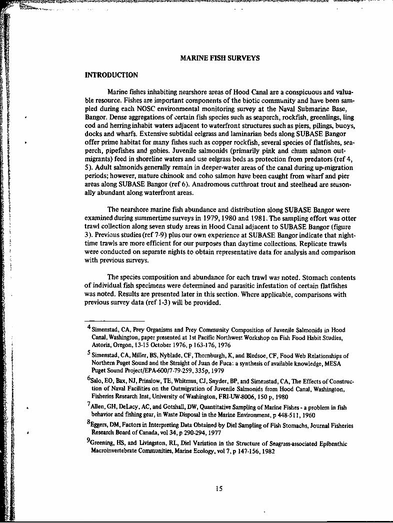
Marine fishes inhabiting nearshore areas of Hood Canal are a conspicuous and valua-ble resource. Fishes are important components of the biotic community and have been sam-pled during each NOSC environmental monitoring survey at the Naval Submarine Base,Bangor. Dense aggregations of certain fish species such as seaperch, rockfish, greenlings, lingcod and herring inhabit waters adjacent to waterfront structures such as piers, pilings, buoys,docks and wharfs. Extensive subtidal eelgrass and laminarian beds along SUBASE Bangoroffer prime habitat for many fishes such as copper rockfish, several species of flatfishes, sea-perch, pipefishes and gobies. Juvenile salmonids (primarily pink and chum salmon out-migrants) feed in shoreline waters and use eelgrass beds as protection from predators (ref 4,5). Adult salmonids generally remain in deeper-water areas of the canal during up-migrationperiods; however, mature chinook and coho salmon have been caught from wharf and pierareas along SUBASE Bangor (ref 6). Anadromous cutthroat trout and steelhead are season-ally abundant along waterfront areas.

The nearshore marine fish abundance and distribution along SUBASE Bangor wereexamined during summertime surveys in 1979, 1980 and 1981. The sampling effort was ottertrawl collection along seven study areas in Hood Canal adjacent to SUBASE Bangor (figure3). Previous studies (ref 7-9) plus our own experience at SUBASE Bangor indicate that night-time trawls are more efficient for our purposes than daytime collections. Replicate trawlswere conducted on separate nights to obtain representative data for analysis and comparisonwith previous surveys.

The species composition and abundance for each trawl was noted. Stomach contentsof individual fish specimens were determined and parasitic infestation of certain flatfisheswas noted. Results are presented later in this section. Where applicable, comparisons withprevious survey data (ref 1-3) will be provided.

4 Simenstad, CA, Prey Organisms and Prey Community Composition of Juvenile Salmonids in HoodCanal, Washington, paper presented at 1st Pacific Northwest Workshop on Fish Food Habit Studies,Astoria, Oregon, 13-15 October 1976, p 163-176, 1976

5 Simenstad, CA, Miller, BS, Nyblade, CF, Thornburgh, K, and Bledsoe, CF, Food Web Relationships ofNorthern Puget Sound and the Straight of Juan de Fuca: a synthesis of available knowledge, MESAPuget Sound Project/EPA-600/7-79-259,335p, 1979

6Salo, EO, Bax, NJ, Prinslow, TE, Whitmus, CJ, Snyder, BP, and Simenstad, CA, The Effects of Construc-tion of Naval Facilities on the Outmigration of Juvenile Salmonids from Hood Canal, Washington,Fisheries Research Inst, University of Washington, FRI-UW-8006, 150 p, 1980

7Alen, GH, DeLacy, AC, and Gotshall, DW, Quantitative Sampling of Marine Fishes - a problem in fishbehavior and fishing gear, in Waste Disposal in the Marine Environment, p 448-511, 1960

8Eggers, DM, Factors in Interpreting Data Obtained by Diel Sampling of Fish Stomachs, Journal FisheriesResearch Board of Canada, vol 34, p 290-294, 1977

9Greening, HS, and Livingston, RL, Diel Variation in the Structure of Seagrass-associated EpibenthicMacroinvertebrate Communities, Marine Ecology, vol 7, p 147-156, 1982

15

N .-N

r ~ ~ r ~ -

....... x. . . . . . . . . . . . ... ... ...

........ii -K - ....

... Point attai

Brown. Hoo ExplsivePoin Caa.HnligHutr

-- i-ix.BANGORO

-""PENService

X. X.4...... . .

...... ..... .....

F oigue3. Ot e trawlnamlin loat dions adjacent. to. SU A EBno.

Ligh6

MATERIALS AND METHODS

Replicate otter trawl samples were taken at stations A, C, D-E, I, J-K, M and Z (seefigure 3 for locations) during summer nighttime hours in 1979, 1980 and 1981. The spread-board otter trawl had a 5-metre mouth opening, two 31.5 x 60cm boards weighing 8 kilo-grams each, a bag of 28-mm stretch mesh, and a cod end of 13-mm stretch mesh. Ten-minutehauls were made from a 16-foot outboard-powered boat at a speed of approximately 1metre/second (2 knots). Each trawl haul sampled about 650 metres of bottom linearly. Aboat-mounted fathometer was used to maintain the trawl at 5-8 metres. That depth rangecorresponds to the deep side of the eelgrass beds and the shallow edge of the laminarianzone at each station. Most trawling was done over sandy substratum.

After each trawl, fish were separated from invertebrates, algae, eelgrass, rocks andshell debris, placed in labeled zip-lock or mesh bags (depending upon size of fish specimens)and returned to the laboratory in an ice-filled cooler for analysis. Adult fishes were identifiedto species in the onsite laboratory using taxonomic references for the region (ref 10-12). Animportant distributional checklist for Hood Canal fishes is found in reference 13.

Fish were identified, separated into species groups, counted, measured and weighed..Length was taken to the nearest millimetre as either fork or total length, depending on thespecies. Weights were determined to the nearest gram. Fish were examined for sex, maturity,parasites or other abnormalities and pertinent data were recorded. The specimens' physical

condition was indicated by fm erosion, tumois or presence of the parasitic nematode,Philometra americana Costa, 1846. Our previous surveys only observed these encysted para-sites in adult rock sole, Lepidopsetta bilineata (Ayres, 1955) (ref 1-3). Copper rockfish,Sebastes caurinus Richardson, 1845, within the 150-250-mm size range were set aside forheavy metal sample dissections (muscle and liver tissue). Stomach and intestinal tract wereanalyzed for most fishes greater than 175 mm in length. The contents of stomachs and intes-tines were visually examined using a variable power (7-70X) binocular dissecting microscope.Identifiable prey organisms or other material were recorded for each specimen examined.,Fishes or prey species which could not be positively identified on site were preserved in 10%formalin-seawater solution.These specimens were taken to NOSC and, if necessary, deliveredto specialists for final identification. A representative reference collection of Hood Canalbiota is maintained at the NOSC Sample Processing Center in Hawaii.

10 Hart, JL, Pacific Fishes of Canada, Fisheries Research Board of Canada Bulletin 180, 740p, 197311 Miller, DJ and Lea, RN, Guide to the Coastal Marine Fishes of California, California Dept. of Fish and

Game Fish Bulletin 157,235 p, 197212 Clemens, WA, and Wilby, GV, F~shes of the Pacific Coast of Canada, 2d ed, Fisheries Research Board of

Canada Bulletin 68,443p, 196113 DeLacy, AC, Miller, BS and Borton, SF, Checklist of Puget Sound Fishes, College of Fisheries,

University of Washington Contr 371, 43p, 1972

17

RESULTS AND DISCUSSION

During 1979, 1980 and 1981 monitoring surveys, more than 2000 individual speci-mens representing 37 species from 18 families of fishes (see table 2) were collected by ottertrawl sampling. The 10 most commonly sampled species (listed in decreasing order of nu-merical abundance) were: english sole (Parophrys vetulus), copper rockfish (Sebastescaurinus), shiner perch (Cymatogaster aggregata), striped seaperch (Embiotoca lateralis),rock sole (Lepidopsetta bilineata), padded sculpin (Artedius fenestralis), C-O sole (Pleuro-nichthys coenosus), plainfm midshipman (Porichthys notatus), Pacific tomcod (Microgadusproximus) and bay pipefish (Syngnathus leptorhynchus). Three other common species, tube-snouts (Aulorhynchus flavidus), three-spine sticklebacks (Gasterosteus aculeatus) and tad-pole sculpins (Psychrolutes paradoxus) were recorded as too numerous to count (TNTC)during several sampling periods; therefore, exact numerical data are not available for thesespecies (table 3).

Five new species of fishes were added to the Trident survey cumulative checklistduring 1979 and 1980 field studies. These species were: Porichthys notatus, Gadus macro-cephalus, Artedius lateralis, Agonus acipenserinus and Citharichthys sordidus. All of thesespecies have been reported previously from Hood Canal (ref 13).

Survey data show that fish abundance and distribution fluctuated from survey tosurvey. Catches were large at most stations during 1979 and 1980 surveys. However, duringthe 1981 survey, fish abundance was markedly reduced. The 1981 survey was conductedearlier in the year (May-June) than previous annual surveys (late June-July), which may par-tially explain the observed reduction in fish abundance. Additionally, only a single trawl wastaken at stations A, D-E, J-K and M during 1981. Divers' qualitative observations adjacent tounder%% ater structures during 1979, 1980 and 1981 indicate an enhanced abundance formany species. Increased piling surfaces provide additional epifaunal habitat and concomitantincreases in fish abundance around pier and wharf areas. Habitat enhancement for many spe-cies has occurred along SUBASE Bangor during the last five years, but many of these water-front areas cannot be sampled with an otter trawl because of subsurface obstructions andunderwater debris. Thus, the otter trawl catch data provide information on fish species in-habiting unobstructed shoreline areas, primarily eelgrass and laminarian habitats. Ottertrawl sampling methods remained consistent during 1979, 1980 and 1981 monitoring surveys;,results compare with previous surveys, even though fish collections during the 1973-1978period were from daytime trawls only. Daily catch records for the 1979-1981 fish trawl col-lections are listed in appendix B.

The 1979 trawl samples took 1199 individual fishes representing 31 species from 16families. The samples were from one daytime and two nighttime trawl series. The daytimetrawls collected 217 individuals representing 13 species from 9 families. Nighttime trawlswere more productive. Night trawl series data are summarized in table 3. Two trawls weretaken at each station on two separate nights, approximately one week apart. Annual trawldata are given in table 4. During the 1980 survey, 840 individuals representing 30 speciesfrom 15 families were collected.

18

Family Genus/Species/Authority/Date Common Name

Squalidae Squalus acanthias Linnaeus, 1758 Spiny DogfishChimaeriidae Hydrolagus colliei (Lay & Bennett, 1839) RatfishBatrachoididae Porichthys notatus Girard, 1854 Plainfin MidshipmanGadidae Gadus macrocephalus Tilesius 1810 Pacific Cod

Merluccius productus (Ayres, 1855) Pacific HakeMicrogadus proxbnus (Girard, 1854) Pacific Tomcod

Aulorhynchidae Aulorhynchusflavidus Gill, 1861 TubesnoutGasterosteidae Gasterosteus aculeatus Linnaeus, 1758 Threespine SticklebackSyngnathidae Syngnathus leptorhynchus Girard, 1854 Bay PipefishEmbiotocidae Cynatogaster aggregata Gibbons, 1854 Shiner Perch

Embiotoca lateralis Agassiz, 1854 Striped SeaperchRhacochilus vacca (Girard 1855) Pile Perch

Stichaeidae Anoplarchus purpurescens Gill, 1861 High CockscombLumpeneus sagitta Wiilmovsky, 1956 (Pacific) Snake Prickleback

Pholidae Apodichthysflavidus Girard, 1854 Penpoint GunnelPholis laeta (Cope, 1873) Crescent GunnelPholis ornata (Girard, 1854) Saddleback Gunnel

Ammodytidae Ammodytes hexapterus Pallas, 1811 Pacific Sand LanceGobiidae Coryphopterus nicholsi (Bean, 1881) Blackeye GobyScorpaenidae Sebastes caurinus Richardson, 1845 Copper RockfishHexagrammidae Hexagrammos stelleri Tilesius, 1809 Whitespotted GreenlingCottidae Artediusfenestralis Jordan & Gilbert, 1882 Padded Sculpin

Artedius lateralis (Girard, 1854) Smoothhead SculpinClinocottus acuticeps (Gilbert, 1895) Sharpnose SculpinEnophrys bison (Girard, 1854) Buffalo SculpinHemilepidotus hemilepidotus (Tilesius, 1810) Red Irish LordLeptocottus armatus Girard, 1854 Pacific Staghorn SculpinNautichthys oculofasciatus (Girard, 1857) Sailfin SculpinPsychrolutes paradoxus Gunther, 1861 Tadpole SculpinScorpaenichthys marmoratus (Ayres, 1854) Cabezon

Agonidae Agonus acipenserinus Tilesius, 1811 Sturgeon PoacherBothidae Otharichtlhys sordidus (Girard, 1854) Pacific SanddabPleuronectidae Lepidopsetta bilineata (Ayres, 1855) Rock Sole

Parophyrs vetulus Girard, 1854 English SolePlatichthys stellatus (Pallas, 1811) Starry FlounderPleuronichthys coenosus Girard, 1854 C-O SolePsettichthys melanostictus Girard, 1854 Sand Sole

Table 2., List of Hood Canal fishes .ollected during Trident environmentalmonitoring surveys (1979, 1980 and 1981).

--4 (Taxonomy based on Hart, 1973.)

19

Station

Species A C D-E J -K M4 Z

'79 180 '81w '79 '80 '81 '79 '80 1810 '79 '80 '81 '79 '90 'Si1 '79 '80 '81* '79 I8o '81

Squaha acanthias 1 2 1 1 i - - - -

Hydbolagua colilei 2 2---------------------2 --- 2 2 - ~-- 3 1 - -

Porichthys notatut 33 5----------------------------------- 4 - ---

Gadur nme~oephahs------------------------------ - - ---- ---------- - - - -

Meluccdus productus 9---------------------------------2

MicrgadusProximuS - 1 5 3 - 19 12 2 15 2 - - - -

Auiorhynchusffavidu 2 4 -TNT- -4 1 - 3 1 - TNTC 1 1 326 - 1- -

Gasterosteusaculealus TNTC 1 ------------------- ----- 2- - - - - - -

Syngnathus leprorhynchus 40- 1- 1 - -- - -3

Cymatog- asterapgta 291i- 7-5 91 -12 1 15 31 5- 26 42 6--6

Embiotoca latemlis 69 3- 4-- S-- 4 2 8 3 - - 7 -- 1-

Rhacochilus vacca 1 1 3 - - - 1

Anopiarchus purpurescens - I 1

Lumpeneussaitta---------------------------------- 1 5 - 514-

Apodichthysflavidus 1 -- 1 1- 2 1----------------1-Pholiskefea 563 1-------------I13Pholis ornata 7----- --------- 1 - 1 2 3 - - -1

A mmodytes hexapterus----------I------------------------------1-

Coryphopterus niholsi I-------------------------------

Sebastes courinus 179 49 11 18 14 412 5 9 8 23 4 18 8 2- 2-2726 4

Hexagrammosstefleri 2 -1 - - I- - 1

Artediusfenestra&i 35 1 I- - 5--- 2 7 13 -1I- 1 2- -

Artedhisilateraiis - 1 -- -- - -- --- 1 - 1 2 - - 3 - - - -

Clinocottus acuticeps------------------------------------------4 -- - -

Enophrys bion 19 2------------------------------------- - -

Hemilepidotus hemilepidotux---- -------------------------

Leptocottus armtus 14 2 -2- 3- 2 - 1 4 - 1 2- 1--

Nautichthys oculofasciatus 1 1--- ------- --------- 3 5 - 1 2 1

Psychrolutes paradoxus-----------------------5 - -TNTC -TNTCTNTC - 2 29- - -

Scorpaenichthys marmoratus 2 1---------------------------------11-

Agonus acpenserinus----------------------------- --- ----- 1

Citharichthys jo'didus-----------------------3 -- 1 7 -1 233 - --

tLepkiopsetta bfiineata - 301 -1 1 1 12 -1 458- 2 1

Parophrys Petulus 7 8 -3 3 34 2 6 1 42 12 - 4732214 -2 2

Plaiichthys stellatus 15 -- 2----------------------------------------- - - -

Pleuronichthys coenosus 9 10--- --- --- --- --- ---------- I 2 7 1 - - - -

Psettichu'hys melanostictus-------------------------------------------18 - - - -

*single trawl data.TNTC =Too numerous To Count

Table 3. Summarized otter trawl data (1979, 1980 and 198 1).

20

Year

1979 1980 1981 Mean/

Station 1 2 1 2 1 2 Station %

A 171 (24) 363 41 (17) 83 14 (4) - 134.4 35

C 33 (11) 7 9 (5) 385 5 (4) 8 12.3 4

D-E 21 (10) 24 12 (7) 6 11 (2) - 14.8 4

1 17 (14) 30 25 (13) 30 0 (9) 35 22.8 7

J-K 66 (21) 85 31 (18 65 9 (7) - 51.2 13

M 56 (13) 55 109 (14) 385 31 (6) - 127.2 33

Z 19 (11) 26 16 (5) 16 1 (3) 6 14.0 6

Totals - 383 590 243 597 71 49 1933+ 100

Means-' 486.50 420.00 60.00

Table 4. Data summary for nighttime otter trawls conducted at SUBASE Bangor during 1979, 1980, and 1981,, Numbersof individuals listed for each of two trawling periods; number of species (in parentheses) combined year totals.

q21

Certain stations consistently provided greater catches: A, M, J-K and I, provided35%, 33%, 13% and 7% of the three-year combined mean trawl catch, respectively. Thesefour stations account for 88% of the total catch during the three-year period. Each of thesestations possesses a well-developed eelgrass and laminarian zone habitat.

Eight fish species were ubiquitous, ie collected at each otter trawl sampling station,during the 1979-1981 survey period. These species are Aulorhynchus flavidus, Cymatogasteraggregata, Embiotoca lateralis, Sebastes caurinus, Artedius fenestralis, Leptocottus armatus,Lepidopsetta bilineata and Parophrys vetulus. These species are typical of Hood Canal andrepresent a healthy nearshore marine environment.

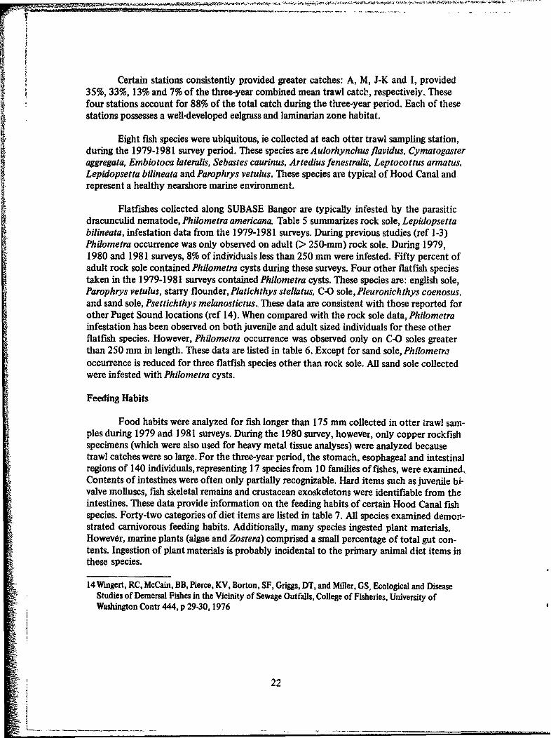
Flatfishes collected along SUBASE Bangor are typically infested by the parasiticdracunculid nematode, Philometra americana. Table 5 summarizes rock sole, Lepidopsettabilineata, infestation data from the 1979-1981 surveys. During previous studies (ref 1-3)Phiometra occurrence was only observed on adult (> 250-mm) rock sole. During 1979,1980 and 1981 surveys, 8% of individuals less than 250 mm were infested. Fifty percent ofadult rock sole contained Philometra cysts during these surveys. Four other flatfish speciestaken in the 1979-1981 surveys contained Philometra cysts. These species are: english sole,Parophrys vetulus, starry flounder, Platichthys stellatus, C-O sole, Pleuronichthys coenosus,and sand sole, Psettichthys melanostictus. These data are consistent with those reported forother Puget Sound locations (ref 14). When compared with the rock sole data, Philometrainfestation has been observed on both juvenile and adult sized individuals for these otherflatfish species. However, Philometra occurrence was observed only on C-O soles greaterthan 250 mm in length. These data are listed in table 6. Except for sand sole, Philometraoccurrence is reduced for three flatfish species other than rock sole. All sand sole collectedwere infested with Philometra cysts.

Feeding Habits

Food habits were analyzed for fish longer than 175 mm collected in otter trawl sam-ples during 1979 and 1981 surveys. During the 1980 survey, however, only copper rockfishspecimens (which were also used for heavy metal tissue analyses) were analyzed becausetrawl catches were so large. For the three-year period, the stomach, esophageal and intestinalregions of 140 individuals, representing 17 species from 10 families of fishes, were examined.,Contents of intestines were often only partially recognizable. Hard items such as juvenile bi-valve molluscs, fish skeletal remains and crustacean exoskeletons were identifiable from theintestines. These data provide information on the feeding habits of certain Hood Canal fishspecies. Forty-two categories of diet items are listed in table 7. All species examined demon-strated carnivorous feeding habits. Additionally, many species ingested plant materials.However, marine plants (algae and Zostera) comprised a small percentage of total gut con-tents. Ingestion of plant materials is probably incidental to the primary animal diet items inthese species.

14 Wingert, RC, McCain, BB, Pierce, KV, Borton, SF, Griggs, DT, and Miller, GS, Ecological and DiseaseStudies of Demersal Fishes in the Vicinity of Sewage Outfalls, College of Fisheries, University ofWashington Contr 444, p 29-30, 1976

22

Survey > 2MOmm # Infested % <250mm # nfested %

1979 (X) 1 1 100 3 1 33

1980 (X) 17 9 53 36 2 6

1981 (XI) 2 0 0 9 1 11

Totals 20 10 48 4

Table 5.. Rock sole infestation by Philometra americana.

Species Survey >250mm # Infested % <250mm # Infisted %

English 1979 (IX) 19 1 5 96 5 5Sole 1980 (X) 9 2 11 349 5 1

C-O Sole 1980 (X) 5 2 40 13 0 0

Starry 1979 (IX) 15 2 7 2 2 100Flounder

Sand 1980 (X) 9 9 100 6 6 100Sole

Table 6. Flatfish other than rock sole infested by Philometra americana.

23

].ii i~ý E

E Ei 'IA'SI Z C its

Apodkchtkysfw•u(l) 265 00 1 0

Dnblotocakeg/~ub(2) 254 0 1I 1 0

F•noprysbiso0(1) 246 1.0:0 0

Hexwgummosseilesl(4) 289 0.4.0 0 • 00• **0 • • •

Hydwliguwcoilie(9) 562 ! 8.-0 0 se * 6 0

Lepidpse,, bilbwsta (7) 269 2.50 0 @0 0 •

Leptoconlusewuu(6) 221 23'1 0 0 0 0 0 0

Lrpga(l) 262 0'17"0 U 0 0 M

Ap'dhccufductusO(1) 317 0 10O 1

Mbi-tockfed• xbn(4) 201 0.20 1 •O•*•

NautLk~thysoadoj/ucias(1) 168 001 l 0

AwpAm/ s~'etula(26) 259 3815 0 0. 0 • 0. *oo o @0 @ • •

flattckhhy~teIma(aQt 294 3'3:1 0 0 S . •e • • .

RnopAwukys coenosi (2) 265 0:0.2 0

Scorepd thysamnoefhwa (4) 442 2.20 00 000 0

Sebautesauwtu-(52) 225 2820.4 3 a 60 0 . *.********* *

,umoha acnnts (3) 624 1.2.0 0 0 0 0

Table 7, Diet categories for selected fishes collected adjacent to SUBASE Bangor inHood Canal during 1979, 1980 and 1981 surveys.

24

Table 7 summarizes the results of the food habit analyses. The larger dots representmajor food items obstrved in more than 50% of specimens of a given species; small dots in-dicate less frequently consumed items. Feeding habits for many of the species listed in table7 have been repoited previously (ref 1-3). The feeding habits of fishes examined during1979-1981 surveys are in general agreement with data from previous SUBASE Bangor sur-veys (1973-1978). Food habit analysis shows ecosystem complexity and interdependenceof biotic relationships within the food webs of nearshore marine biota along SUBASEBangor. Crustaceans were the principal diet items in fish guts analyzed during these surveys.

Other major groups of diet items include: fishes, polychaete worms and bivalve molluscs.

Copper Rockfish (Sebastes caurinus)

Copper ro". fish guts typically contained crustaceans, especially the shrimp, Pandalusdanae, and other fishes. Sebactes caurinas is a faculative feeder which consumes a wide vari-ety of food items present in the nearshore eelgrass beds and piling habitats along HoodCanal. Reference 15 describes similar feeding trends by copper rockfish from southern PugetSound. Twenty food item categories were found in the guts of this species. Reference 16 ex-amined food habits of Sebastes caurinus in southern Humboldt Bay, northern California andcategorized copper rockfish as opportunistic carnivores. Our Hood Canal data support thisdescription. Copper rockfish feed most actively at night and early morning hours (ref 15;observations during this study).

English Sole (Parophrys vetulus)

English sole consumed clam siphon tips and polychaete worms as major diet items.However, many other types of food items were identified from stomach anid intestine analy-ses. English sole was the most frequently collected species during this survey period. We col-lected 480 individuals, mostly juveniles, ie < 100 mm, English sole apparently feed at night.English sole is the only species we sampled that fed on ophiuroids (brittle stars). During pre-vious surveys (1973-1978) rock sole was the only species which contained ophiuroids.

Pacific Hake (Merluccius productus)

Pacific hake stomachs contained herring and, in one instance, juvenile chum salmon.These diet items were found in the stomachs of 10 specimens collected during the 1979 sur-vey. Hake are nocturnal feeders, based upon observations made during this study and thosereported elsewhere (ref 10).

Ratfish (Hydrolagus colliei)

Ratfish exhibited a preference for crabs as diet items; however, several specimensexamined contained fish remains, barnacles, stlrimn,, marine plants and shell debris. These

15 Patten, BJ, Biological lIformation on Copper Rockfish in Puget Sound, Washington, Trans Am FisheriesSociety, vol 102, p 412-416, 1973

16 Prince, ED, Food of the Copper Rockfish, Sebastes caurinus Richardson, Associated with an Artificial

Reef in South Humboldt Bay, California, California Fish and Game, vol 62, p 274-285, 1976

25

nocturnal predators were often collected in pairs, although eight out of nine specimens col-lected were females.

Rock Sole (Lepidopsetta bilineata)

Rock sole fed primarily on molluscs. Major diet items consisted of bivalve siphontips and juvenile basket cockles. Polychaete worms were less frequent in rock sole stomachs.Reference 17 lists polychaetes and sandlances as principal diet items for rock sole in HecateStrait, north of Vancouver Island, British Columbia.

Starry Flounder (Platichthys stellatus)

Starry flounder ingested clam siphon tips a. a major diet item, This concurs withfood habits for this species reported from Elkhorn Slough, California (ref 18). Polychaetes,small basket cockles and crab fragments were also ide~itified from stomachs and intestines.This species of flatfish contains both right- and left-h .nded individuals. It is interesting thatmost males were observed to be right-handed in Ho.,d Canal collections during this surveyperiod.

Pacitic Staghom Sculpin (Leptocottus armatus)

Pacific staghorn sculpin are voracious feeders (ref 10). Shiner seaperch, shrimp andcrabs were major diet items for this species. Anemones were also common in stomachs.Other fishes, eelgrass and pea gravel occurred less frequently in Leptocottus armatus feedinghabits.

Whitespotted Greenling (Hexagrammos stelleri)

Whitespotted greenling fed primarily on the shrimp, Pandalus danae; however, manyother diet items were identified from four female specimens examined during this period.Hexagrammos stelleri were collected from unobstructed eelgrass and laminarian zone habit-ats at stations A, D-E and I during the 1979 survey.

Pacific Tomcod (Microgadus proximus)

Pacific tomcod were common in otter trawl samples from the northern samplingstations 1, J-K and M. Only four individuals larger than ! 75 mm were examined for foodhabit analysis during 1979, 1980 and 1981 surveys. The primary diet item for this speciesconsisted of skeleton shrimp. Also polychaetes, shrimp and amphipods were ingested to alesser extent. Little is known about the life history of this species in Puget Sound (ref 10).

17 Forrester, CR, and Thompson, JA, Population Studies on the Rock Sole (Lepidopsetta bilineata) ofNorthern Hecate Strait, British Columbia, Fisheries Research Board of r nada Tech Report 108,104p, 1969

18 Orcutt, HG, The Life History of the Starry Flounder, California Def n and Game Fish Bulletin78, 64p, 1950

26

Cabezon (Scorpaenichthys marmoratus)

Cabezon fed chiefly on the red rock crab, Cancer productus, Specimens examinedduring this period also contained gunnels, cabezon eggs, miscellaneous crustacean fragmentsand marine plant debris. Cabezon were only collected from the two southernmost stations,A and Z.

Spiny Dogfish (Squalus acanthias)

Spiny dogfish sharks consumed ctenophores, fishes and shrimp. Seldom collectedin otter trawls, this active carnivore was mainly present in trawls from northern stationsalong SUBASE Bangor. Reference 19 reported that in British Columbia waters, principallyin the Strait of Georgia, spiny dogfish feed on Pacific herring, euphausids, unidentified eggsand caridean crustaceans during all combined life stages.

The remaining six species were represented by only one or two specimens for exam-ination., Therefore, general comments regarding food habits during this survey period are notprovided for these fishes. An excellent synthesis and summary of available knowledge con-cerning food web relationships of northern Puget Sound and the Strait of Juan de Fuca canbe found in reference 5..

CONCLUSIONS

1. Fish abundance and distribution data collected during 1979, 1980 and 1981 sur-veys indicate that ichthiofauna along SUBASE Bangor are typically diverse and demonstratecharacteristically healthy assemblages.

2. Increased nearshore habitat resulting from additional waterfront structures alongHood Canal at SUBASE Bangor supports numerically enhanced assemblages of many marinefish species.

3. Nighttime otter trawl collections provide a quantitative, reliable and cost-effectivemeans to monitor marine fish fauna along SUBASE Bangor on an annual basis.

4. Philometra americana, a parasitic nematode, infested five common flatfish speciesinhabiting nearshore environments adjacent to SUBASE Bangor.,

5. Diverse feeding habits were recorded for 17 common Hood Canal fish species.Crustaceans, fishes, polychaete worms and bivalve molluscs were predominant food itemsfor fishes examined during this period.

6. The distribution and composition of marine fish assemblages at SUBASE Bangorhave not shown adverse characteristics attributable to %.onstruction effects during the period1979-1981.

19Jones, BC, and Geen, GH, Food and Feeding Habits of Spiny Dogfish (Squalus acanthias) in BritishColumbia Waters, Journal Fisheries Research Board of Canada, vol 34, p 2067-2078, 1977

27

INTERTIDAL SURVEYS

INTRODUCTION

Regions of tidal influence are important components of most marine ecosystems.Nearshore intertidal regions: 1) provide nursery areas, food and habitat for many species ofvertebrates and invertebrates; 2) are primary sites for nutrient cycling; 3) offer maximumavailable sunlight for photosynthetic activity; and 4) often support dense aggregations ofeconomically important species of marine flora and fauna in a location that makes themavailable for human consumption. These legions of diverse, interdependent biotic assem-blages are also susceptible to man-induced impacts such as resource removal (harvesting),habitat alteration and pollutant stresses. Intertidal environmental monitoring is warrantedby economic, recreational and aesthetic values. These potentially impacted regions are eco-logically important to the entire marine ecosystem.

Shoreline intertidal regions in Puget Sound are highly productive zones. At theSUBASE Bangor study area located along northern Hood Canal (see figure 2), certain inter-tidal transect sampling stations have been monitored annually since 1973 (ref 1-3). Centralto monitoring efforts have been annual evaluations of recreationally, commercially andecologically important species of marine bivalve molluscs, especially clams, oysters andmussels.

Bivalve Molluscs

Bivalve molluscs are sedentary or sessile, filter-feeding organisms which remain in aspecific localized intertidal area. They dominate the biomass of intertidal regions in PugetSound. These important marine organisms respond to environmental conditions present in agiven locale. Their usefulness in monitoring studies is determined by measurable, albeitoften subtle, responsiveness to environmental perturbations. The recreational and commer-cial importance of certain bivalve molluscs in Puget Sound is well established (ref 20-24).

This section presents distribution and density data for the following species of bi-valves along SUBASE Bangor: Saxidomus giganteus (Deshayes, 1839), butter clam;

20Amos, MH, Commercial Clams of the North American Pacific Coast, Bureau of Commercial Fisheries

Circular 237, 18p, 196621Chew, KK, Prospects for Successful Manila Clam Seeding, College of Fisheries, University of Washington

Contr 440, 13p, 197522Magoon, C, and Vining, R. Introduction to Shellfish Aquaculture in the Puget Sound Region, Division of

Marine Land Management, Washington Dept of Natural Resources, 68p, 198123Quayle, DB, Distribution of Introduced Marine Mollusca in British Columbia Waters, Journal Fisheries

Research Board of Canada, vol 21, p 1155-1181, 19642*Westley, RE, The Oyster Producing Potential of Puget Sound, Proc. National Shellfisheries Assoc, vol 61,

p 20-23, 1971

28

- V,• • €,•: , - '- ______. ________________________-

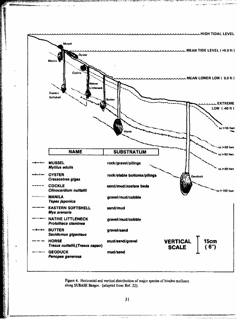
Protothaca staminea (Conrad, 1837), native littleneck clam; Tapes* japonica Deshayes,1853, Japanese or Manila littleneck clam; Clinocardium nuttallii (Conrad, 1837), basketcockle; Mya arenaria Linnaeus, 1758, eastern softshell clam; Tresus capax (Gould, 1850)and Tresus nuttallii (Conrad, 1837), horseneck or gaper clams;Panopea generosa (Gould,1850), geoduck clam; Crassostrea gigas (Thunberg, 1795), giant Pacific or Japanese oysterand Mytilus edulis Linnaeus, 1758, bay mussel. Figure 4 depicts the typical horizontal andvertical distribution and range of these species of bivalve molluscs along SUBASE Bangor.Geoduck and horseneck clams primarily occur subtidally throughout Puget Sound. Thesespecies are included in this section because they have been observed and collected duringintertidal sampling along SUBASE Bangor shorelines. Subtidal distributional data for thesespecies were reported previously (ref 1,2). Many other species of bivalve molluscs were col-lected during field surveys; however, due to their small size or undesirability as a source offood, these species are not considered recreationally or commercially important. Ecologi-cally, many of these species are significant to functional aspects of the Hood Canal marineecosystem.

MATERIALS AND METHODS

Intertidal transect sampling was performed at stations A, Z, C, D, G and J during1979, 1980 and 1981 surveys. Additionally, station M, off-base to the north, was sampledonly during 1979. As discussed previously, data from this station were not considered repre-sentative for the area, and, therefore, station M was deleted as an intertidal sampling stationin 1980., The locations of NOSC intertidal transect stations at SUBASE Bangor are shown infigure 2; latitude and longitude data for each station are listed in appendix A.

Upon arrival at an intertidal transect station, usually about two hours prior to lowtide, the survey team initially positioned sampling equipment on the beach, located thepermanent high tidal level marker and deployed the transect line on a predetermined magne-tic heading. Intertidal station sampling parameters are listed in table 8. A handheld magne-tic bearing compass (figure 5) was used to position the intertidal transect line along the sameaxis for year to year comparisons of data. Two replicate digs were made along either side of

f the transect line at predetermined marks. The PVC-coated fiberglass transect line is markedin metres and decimetre gradations. Most transects were deployed perpendicular to theshoreline across the intertidal region from extreme high tidal mark to low tide level duringeach day of intertidal sampling. Using the computed time of low tide** and noting the dis-tance along the transect line as a reference point, tidal heights were determined using a beachprofiling technique (ref 26) described in detail previously (ref 3). The selection of distances

*Tapes japonica (Deshayes, 1853) has been referred to by junior synonyms of T. semidecussata and T.

philipinaum and variously placed in Paphia, Venerupis, Protothaca and Ruditapes, now used as asubgenus (ref 25)

**NOSC monitoring surveys were scheduled to coincide with the lowest tides during the sampling month,as listed in NOAA Tide Tables for the year.

25Smith, RI, and Carlton, JT, Ught's Manual: Intertidal Invertebrates of the Central California Coast,3d ed. p 562, University of California Press, 1975

26Emery, KO, A Simple Method of Measuring Beach Profiles, Unmolcgy and Oceanography, vol 6, p 90-93,1966

29

Station Magnetic Approx. Major F/S Distance along lineDesignation Axis Length(m)* Zones** # Digs (m) & F/S Zones***

A 2500/0700 42 3 8 26, 29, 33, 36B2, B2, C3, F6

Z 3050/1250 46 3 8 19,23, 27, 35AB2, B3, B3, C4

C 2700/0900 37 4 8 21,26, 31, 35AB3, B3, D3, E5

D 3220/1420 165 4 10 30, 50, 75, 100, 140A3, B3, D4, D4, F5

G 3100/1300 35 3 8 18, 22, 28, 32C3, C4, F6, F5

J 2900/1100 85 4 10 19, 25, 30, 40, 75B2, B3, B5, D5, FS

M 2600/0800 75 4 8 20, 24, 46, 65AB2, C5, D4, F5

*each transect extends from high water level to mean lowest tidal conditions; lengths and distances in metres.

**Faunal/substrate (F/S) zones (see below):

Faunal Zones Substrate Zones

A-mussel/barnacle 1 -riprapB-oyster 2-boulders/rocksC-shell debris 3-stones/gravelD-ulvoids 4-pea gravel/sandE-sargassum/laminoids 5-sandF-eelgrass 6-mud/sand

***Zero end of transect line is at high tide marker.

Table 8. SUBASE Bangor intertidal station transect parameters during 1979, 1980 and 1981 surveys.

30

--------- HIGH TIDAL LEVEL

Mussel

MEAN TIDE LEVEL (+5.oft)oyster

Manila

------- ....MEAN LOWER LOW(C 0.0 ft)

Softshell Butter

4 to >605 feet

NAME SUBSTRATUM4%, t>60fe

--- MUSSEL rock/gravel/pilingsMytilus edulls to >760 feet

--- OYSTER rock/stable bottoms/pilings edcCrassostrea glgas Godc

----- COCKLE sand/mud/zostera bedsCllnocardlum nuttallll ~to >155 feet

MANILA gravel/mud/cobbleTapes japonicaEASTERN SOFTSHELL sand/mudMys arenarla

-. NATIVE LITTLENECK gravel/mud/cobbleProtothaca stamlneal

--- BUTTER gravel/sandSaxldomus giganteus

--- HORSE mud/sand/gravel VERTICAL 15cmTresus nuttalfll,(Tresus capax) SC L I 61GEODUCK mud/sand APanopea generosa

Figure 4. Horizontal and vertical distribution of major species of bivalve molluscsalong SUBASE Bangor. (adapted from Ref. 22).

31

Figure 5. NOSC field team member sighting intertidal transect line positionusing a hand-held magnetic bearing compass.

32

along the transect line has been determined by major substratum and faunal zone stratifica-tion. Through careful field observations of faunal and substrata types, subtle yet recogniz-able intertidal zonation patterns have been identified along Hood Canal shorelines. Dig loca-tions remained within the same intertidal zones for year-to-year comparisons among surveys.

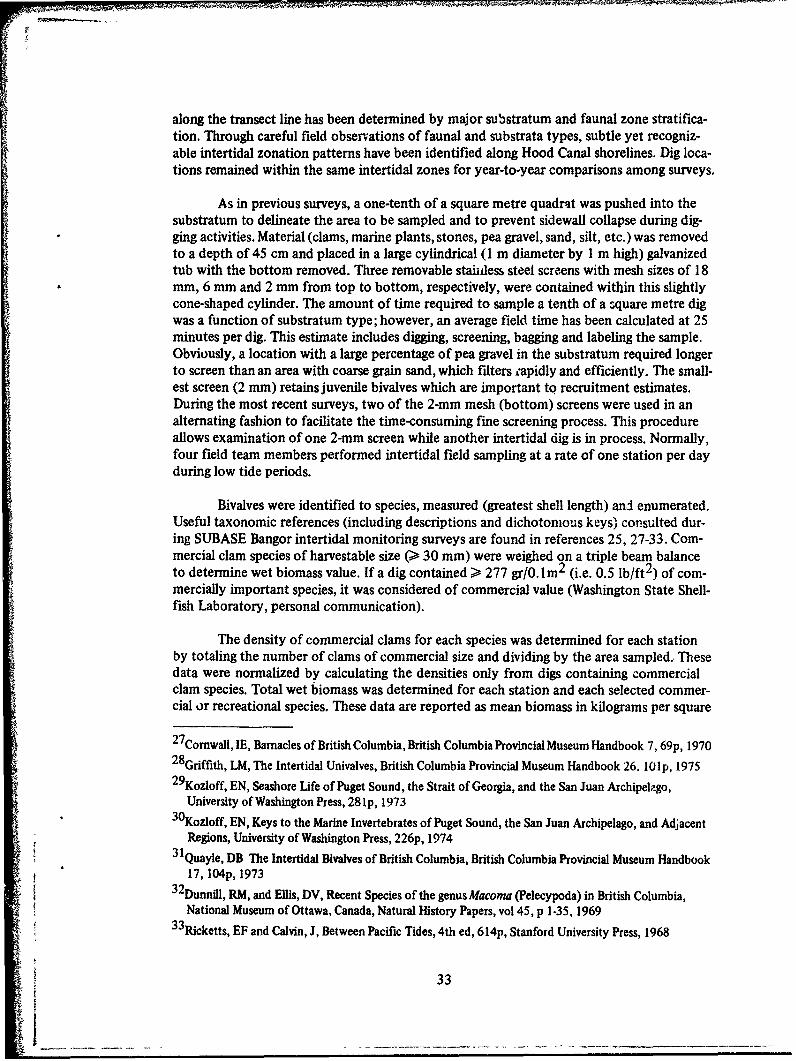
As in previous surveys, a one-tenth of a square metre quadrat was pushed into thesubstratum to delineate the area to be sampled and to prevent sidewall collapse during dig-ging activities. Material (clams, marine plants, stones, pea gravel, sand, silt, etc.) was removedto a depth of 45 cm and placed in a large cylindrical (1 m diameter by 1 m high) galvanizedtub with the bottom removed. Three removable staindess steel screens with mesh sizes of 18

umm, 6 mm and 2 mm from top to bottom, respectively, were contained within this slightlycone-shaped cylinder. The amount of time required to sample a tenth of a square metre digwas a function of substratum type; however, an average field time has been calculated at 25minutes per dig. This estimate includes digging, screening, bagging and labeling the sample.Obviously, a location with a large percentage of pea gravel in the substratum required longerto screen than an area with coarse grain sand, which filters 'apidly and efficiently. The small-est screen (2 mm) retains juvenile bivalves which are important to recruitment estimates.During the most recent surveys, two of the 2-mm mesh (bottom) screens were used in analternating fashion to facilitate the time-consuming fine screening process. This procedureallows examination of one 2-mm screen while another intertidal dig is in process. Normally,four field team members performed intertidal field sampling at a rate of one station per dayduring low tide periods.

Bivalves were identified to species, measured (greatest shell length) and enumerated.Useful taxonomic references (including descriptions and dichotomous keys) consulted dur-ing SUBASE Bangor intertidal monitoring surveys are found in references 25, 27-33. Com-mercial clam species of harvestable size (> 30 mm) were weighed on a triple beam balanceto determine wet biomass value. If a dig contained > 277 gr/O. Im2 (i.e. 0.5 lb/ft 2) of com-mercially important species, it was considered of commercial value (Washington State Shell-fish Laboratory, personal communication).

The density of commercial clams for each species was determined for each stationby totaling the number of clams of commercial size and dividing by the area sampled. Thesedata were normalized by calculating the densities only from digs containing commercialclam species. Total wet biomass was determined for each station and each selected commer-cial or recreational species. These data are reported as mean biomass in kilograms per square

27Cornwall, IE, Barnacles of British Columbia, British Columbia Provincial Museum Handbook 7, 69p, 19702 8Griffith, LM, The Intertidal Univalves, British Columbia Provincial Museum Handbook 26. 101p, 197529Kozloff, EN, Seashore Life of Puget Sound, the Strait of Georgia, and the San Juan Archipelago,

University of Washington Press, 28lp, 197330Kozloff, EN, Keys to the Marine Invertebrates of Puget Sound, the San Juan Archipelago, and Adjacent

Regions, University of Washington Press, 226p, 197431Quayle, DB The Intertidal Bivalves of British Columbia, British Columbia Provincial Museum Handbook

17, 104p, 197332DunnMll, RM, and Ellis, DV, Recent Species of the genus Macoma (Pelecypoda) in British Columbia,

National Museum of Ottawa, Canada, Natural History Papers, vol 45, p 1-35, 196933Ricketts, EF and Calvin, J, Between Pacific Tides, 4th ed, 614p, Stanford University Press, 1968

33

metre for comparative purposes. Additionally, the total number of clams in the commercial(i.e. > 30 mm) and subcommercial (i.e. < 29.9 mm) size ranges was calculated for each spe-cies, dig site and station. The subcommercial category was further subdivided by countingthe number of clams 10 mm or smaller in length. This group consisted of juvenile bivalveswhich settled out of the plankton within the previous year. These young-of-the-year (YOY)data are useful to document recr.itment of important commercial species of bivalves alongSUBASE Bangor.

To enhance statistical validity, a minimum of two replicate digs were performed ateach biological zone (which generally equates to a range of tidal heights). Data from thesesamples were averaged for each tidal region and summarized by species. Intertidal bivalveabundance and density were treated separately by station and by year.

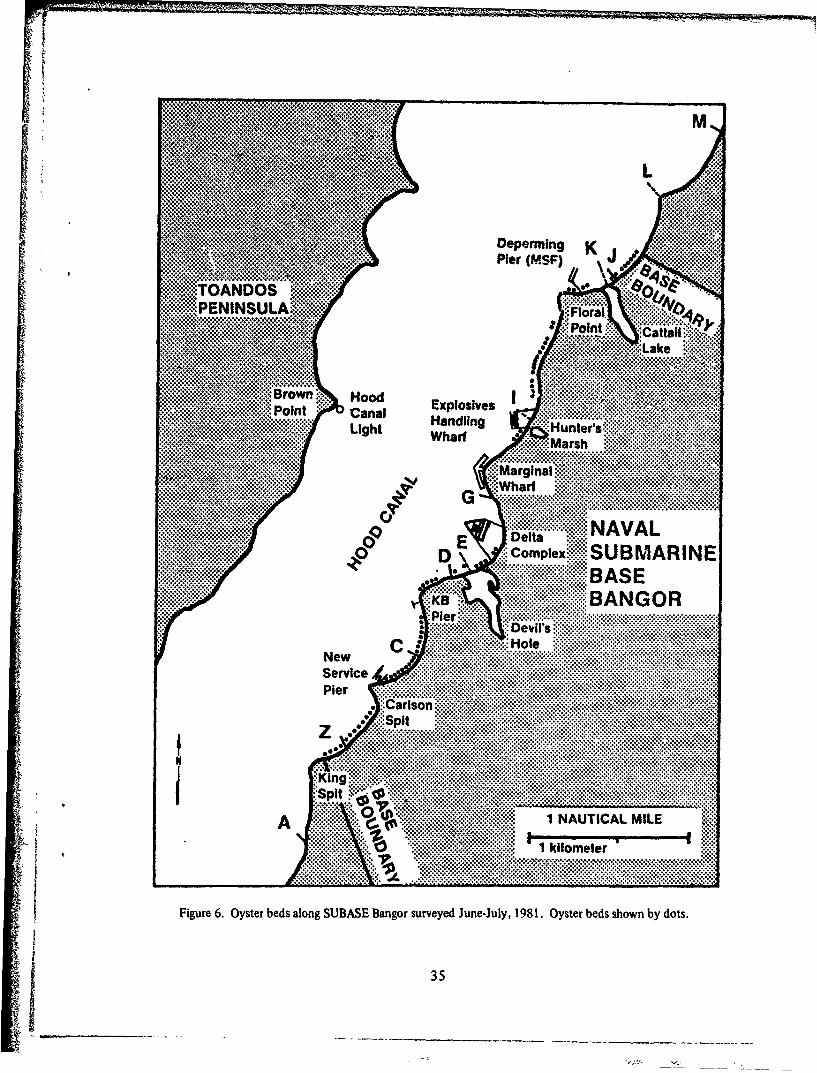
During intertidal transect surveys, oyster abundance data were recorded for oysterspresent in one-tenth of a square metre quadrat samples at each station. Enumeration of oys-ters less than 2 inches (5.08 cm) long and equal to or greater than 2 inches was recorded.Previous surveys (ref 3) established a 2-inch minimum size to differentiate between commer-cial and non-commercial dimensions, a more realistic commercially harvestable size is con-sidered to be 3 inches (7.62 cm). This redefined criterion has been accepted and used bySUBASE Bangor personnel. During June-July 198 1, all existing oyster beds along SUBASEBangor shorelines were surveyed by Mr. Donald Morris and Mr. Edward Cadera, fish andwildlife specialists. Oyster bed length and width parameters were measured using transecttapes. Random samples of oysters contained within a 0.1-square-metre area circular quadratring were counted. Width measurements and random ring toss counts were performed every30 metres along the bed length. Furthermore, at each bed width site, counts were obtainedalong the upper, middle and lower areas of established oyster beds. Numerical data forcommercial-size (equal to or greater than 3 inches) and noncommercial-size (less than 3inches in length) oysters were tabulated and summarized for each site (see figure 6). An oys-ter resource management plan was developed by Don Morris, SUBASE Bangor fish and wild-life specialist, and is included as appendix C.

RESULTS AND DISCUSSION

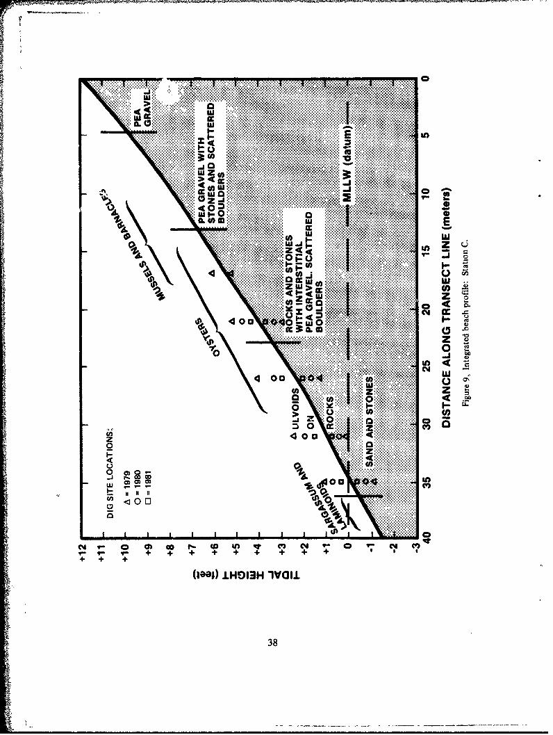
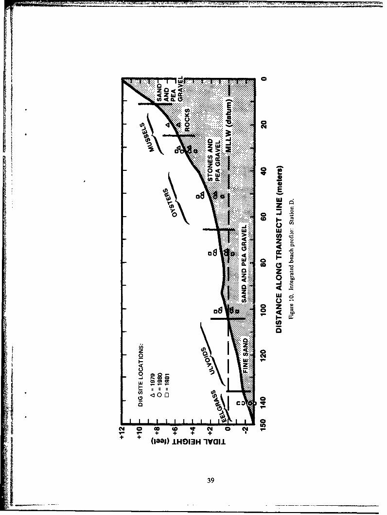
Intertidal bivalve data were collected from seven environmental monitoring stationsalong Hood Canal during 1979, 1980 and 1981 surveys. Station beach profiles, substratatypes, location of dig sites, biotic and tidal reference heights are shown in figures 7 through13. Vertical lines on the figures indicate major substrata delineations. These figures illustratea variety of beach slopes, faunal and floral zonation patterns and types of substrata whichare present along SUBASE Bangor waterfront areas.

Bivalve abundance, distribution and biomass data from 1979, 1980 and 1981 sur-veys are presented in a specific-to-general sequence. Annual bivalve density data, by species,for each tidal height are presented in tables 9 through 15. A discussion of station-specific

intertidal bivalve parameters is followed by summary data which describe combined species,station and yearly survey patterns. Length-frequency data for major bivalve species are listedin appendix D.

34

.:;

X .0 ....

.4, Pier (MSF)

.Cattailx-

Brown Hood EpoiePoint Canal Hadigunes

L S it h Ul_ _ _ _ _ _

.......... ......................................... .

. . . . . . . . . . . ....... . . . . . . . . . . . .

Figure ~ ~ ~ ~ ~ ~ ~ ... aria 6.Ose.ed.ln.....agrsrvydJn-jl,18.Oytrbd honb os

w Ln

4 00LO

w

d. r > . ......I Iul

.. .I .. ...

tp 0

ZW

2L .. ... %... . . .0 z -~ .-M

....... I.-

0 0.........iZw

40 **o

tpE 4CL

0 C0ol ..... .... ... % V) ~ ci '- 0 ' ~ c

'- Y - + + + ++ + V-(~eoj)IHOI3 ivCA

36 L

j ...... ......w. ..... .. .....

d l ...........0. ..... ....... ..

... ... .. .. ..

dl()4............. .......... U...... ... ..

.. .... .........

X~ Z

.0

i z

79

0 z... ... ...

00 ~ 0).. .. .. .-.

.. ........

0 0-

S.- 0 0) 00 (n CM V7~N+ + +

(ION) 1HO13H IVGIIi

37

. .. ................................XXXI

* 10.......~~...................* to

.. . . ......0.

..... .....

I.)4. a a$ B.C>

... ... ... ..9UJ£ ... ........ .... ... .......

....... ...... ... ...

.. .. . .

Z W >o

x0C Ccc..... ....

op 40 0 v.Cc C....

.. ..... CM.. . . . . .. .. ,

........ .....,. ..ou...

. . ...... ..

N i-~~.. .... ...... ) () N ~i~~~1... ........ + + +0

+j ... +..........j ..I3 ........

z 438

z w

().. .....

.. . 0... .

zz

CO)

0.

08

ol Cl

C.,l

0 Cl Ni)

39

Ic

' ....... .... .. ... .. .. ...0.....

ic

1 cc 4c

ch 0

U)

m ZIC-

ZZ

U)U

CMc

400

I ( j o

I-n

CIS'S

.00

co 0 40 c 0 (T + +w+

Oeoi) ~ ~ mozi

41

I?z J

U '.................

.-..

tit ca ......

0 awa

z00

Ck m

00

0 IIn

'p Zo

00

0 CD

0 -I

N 0 g to 0 cm0c

hosi) ~ iLe3nia

"42

Species

Tidal Ht Protothaca Tapes Saxidomus Tresus Tresus Mya Clinocardium(ft)/Year staminea japonica giganteus nuttallli capax arenaria nuttalifi

+2.50/1979 5.00(5.00) 0.00(5.00) NP NP NP NP NP1980 10.00 (0.00) NP 0.00 (10.00) NP NP NP NP1981 0.00 (15.00) NP NP NP NP NP NP

+1.25/1980* 80.00 (45.00) NP 5.00(0.00) N? NP 5.00(0.00) NP1981 15.00 (30.00) NP NP NP NP NP 0.00 (5.00)

0.00/1979 110.00 (25.00) NP 45.00 (25.00) NP NP NP 0.00 (5.00)1980 60.00 (10.00) NP 90.00 (5.00) NP NP NP 0.00(5.00)1981 45.00 (15.00) NP 75.00 (5.00) NP NP NP NP

-0.50/1979 30.00 (25.00) NP 95.00 (35.00) NP 5.00(0.00) NP 0.00 (5.00)1980 40.00 (15.00) NP 195.00 (15.00) NP NP 5.00(0.00) 0.00 (20.00)1981 20.00 (0.00) NP 45.00 (10.00) NP NP NP 0.00 (10.00)

-1.25/1979* 10.00 (20.00) NP 110.00 (0.00) NP - NP NP 5.00 (5.00)

-1.50/1980* 15.00 (0.00) NP 100.00 (0.00) NP 10.00 (0.00) 10.00 (0.00) 0.00 (60.00)

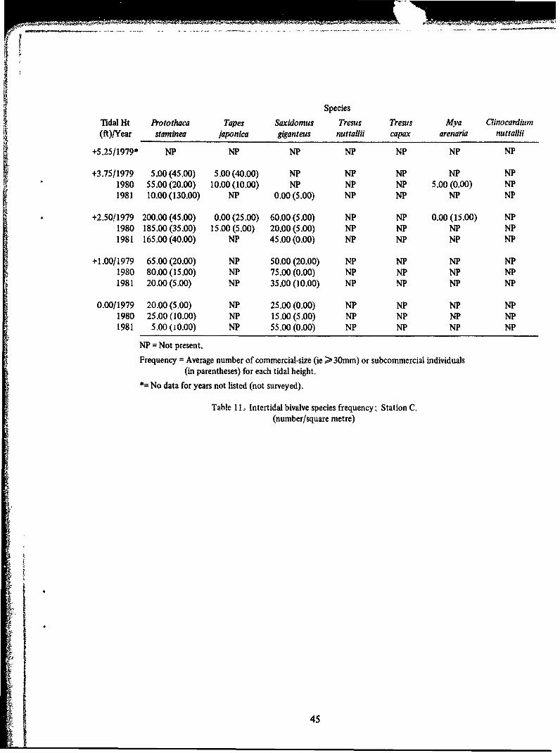
NP = Not present.

Frequency = Average number of commercial-size (ie > 30mm) or subcommercial individuals(in parentheses) for each tidal height.

* No data for years not listed (not surveyed).

Table 9. Intertidal bivalve species frequency Station A.(number/square metre)

43

Species

Tidal Ht Protothaca Tapes Saxidomus Tresus Tresus Mya Clinocardium(ft)fYear staminea japonica giganteus nuttallii capax arenarwa nuttallii

+4.50/1979 30.00 (25.00) 15.00 (160.00) 0.00 (5.00) NP NP NP NP1980 35.00 (45.00) 15.00 (80.00) 5.00 (0.00) NP NP NP NP1981 0.00 (25.00) 5.00(0.00) NP NP NP NP NP

+3.00/1979 55.00(105.00) 70.00 (115.00) 5.00(0.00) NP NP NP NP105.00 (45.00) 15.00 (35.00) 10.00 (0.00) NP NP NP NP50.00 (10.00) NP 10.00 (0.00) NP NP NP NP

+1.75/1979 115.00 (50.00) 20.00 (35.00) 90.00 (5.00) NP NP 5.00(0.00) NP1980 80.00 (15.00) NP 50.00 (0.00) NP NP NP NP1981 50.00 (15.00) NP 45.00 (0.00) NP NP NP NP

0.00/1979 20.00 (0.00) NP 15.00 (5.00) NP NP NP NP1980 5.00(5.00) NP 20.00 (0.00) NP NP NP NP1981 10.00 (5.00) NP 5.00 (15.00) NP NP NP NP

NP = Not present.

Frequency Average number of commercial-size (ie >30mm) or subcommercial individuals(in parentheses) for each tidal height.

Table 10. Intertidal bivalve species frequency: Station Z.(number/square metre)

44

Species

Tidal Ht Protothaca Tapes Saxidomus Tresus Tresus Mya Clinocardium(ft)/Year staminea japonica giganteus nuttallii capax arenaria nuttaiii

+5.25/1979* NP NP NP NP NP NP NP

+3.75/1979 5.00 (45.00) 5.00 (40.00) NP NP NP NP NP1980 55.00 (20.00) 10.00 (10.00) NP NP NP 5.00 (0.00) NP1981 10.00 (130.00) NP 0.00 (5.00) NP NP NP NP

+2.50/1979 200.00 (45.00) 0.00 (25.00) 60.00 (5.00) NP NP 0.00 (15.00) NP1980 185.00 (35.00) 15.00 (5.00) 20.00 (5.00) NP NP NP NP1981 165.00 (40.00) NP 45.00 (0.00) NP NP NP NP

+1.00/1979 65.00 (20.00) NP 50.00 (20.00) NP NP NP NP1980 80.00 (15.00) NP 75.00 (0.00) NP NP NP NP1981 20.00 (5.00) NP 35.00 (10.00) NP NP NP NP

0.00/1979 20.00 (5.00) NP 25.00 (0.00) NP NP NP NP1980 25.00 (10.00) NP 15.00 (5.00) NP NP NP NP1981 5.00 (10.00) NP 55.00 (0.00) NP NP NP NP

NP = Not present.

Frequency = Average number of commercial-size (ie • 30mm) or subcommercial individuals(in parentheses) for each tidal height.

* No data for years not listed (not surveyed).

Table 11, Intertidal bivalve species frequency. Station C.(number/square metre)

45

Species

Tidal Ht Protothaca Tapes Saxidomus Tresus Tresus Mya Clinotardium(ft)/Year stwninea japonica giganteus nuttallii capax arenaria nuttalii

+6.25/1979* NP 10.00 (60.00) NP NP NP 15.00 (15.00) NP

+5.00/1979 120.00 (155.00) 5.00 (10.00) 100.00 (105.00) NP NP NP 0.00(5.00)1980 0.00 (30.00) 75.00 (110.00) 0.00(5.00) NP NP 5.00(0.00) NP1981 0.00 (5.00) 90.00 (5.00) NP NP NP 5.00(5.00) NP

+2.00/1979 35.00 (65.00) NP 45.00 (65.00) NP NP 10.00 (0.00) 15.00 (0.00)1980 90.00 (180.00) 15.00 (10.00) 45.00 (105.00) NP NP NP 0.00 (10.00)1981 20.00 (195.00) 20.00 (5.00) 40.00 (140.00) NP NP 0.00 (5.00) NP

+1.00/1979 75.00 (25.00) NP 185.00 (70.00) NP NP 0.00(5.00) NP1980 55.00 (10.00) NP 45.00 (10.00) NP NP 5.00(0.00) NP1981 55.00 (75.00) NP 50.00 (25.00) NP NP NP NP

0.00/1979 5.00(5.00) NP 25.00 (25.00) NP NP NP NP1980 40.00 (45.00) NP 30.00 (10.00) NP NP NP 15.00 (30.00)1981 25.00 (40.00) NP 55.00 (40.00) NP NP NP 5.00(5.00)

-2.25/1980* 0.00(5.00) NP 55.00 (10.00) NP NP NP 5.00(5.00)1981 15.00 (5.00) NP 45.00 (5.00) NP 5.00 (5.00) NP NP

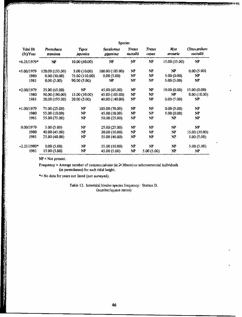
NP = Not present.

Frequency = Average number of commercial-size (ie > 30mm) or subcommercial individuals(in parentheses) for each tidal height.

* No data for years not listed (not surveyed).

Table 12. Intertidal bivalve species frequency: Station D.(number/square metre)

46

Species

Tidal Ht Protothaca Tapes Saxidomus Tresus Tresus Mya Clinocardb.m

(ft)/Year staminea japonica giganteus nuttalihi capax arenaria nuttallhi

+3.00/1979* NP NP NP NP NP NP NP

+1.75/1979 45.00 (0.00) NP 0.00 (15.00) NP NP NP NP1980 20.00 (0.00) NP NP NP NP 5.00(0.00) NP1981 0.00 (15.00) NP 5.00(0.00) NP NP NP NP

+0.75/1979 NP NP NP NP 10.00 (0.00) NP 5.00 (0.00)1980 NP NP 5.00(0.00) NP NP NP 15.00 (5.00)

S1981 5.00(0.00) NP 15.00 (0.00) NP NP NP 0.00 (10.00)

-0.75/1979 5.00 (10.00) NP 20.00 (0.00) 15.00 (0.00) NP NP NP1980 5.00(0.00) NP 5.00 (0.00) NP 5.00(0.00) NP 5.00(5.00)1981 NP NP 25.00 (5.00) 15.00 (0.00) NP NP 5.00(0.00)

-1.50/1979 NP NP 30.00 (5.00) 5.00 (0.00) 5.00(0.00) NP 5.00 (0.00)1980 5.00(0.00) NP 25.00 (0.00) NP NP NP 0.00 (10.00)1981 5.00(0.00) NP 30.00 (10.00) NP 5.00(0.00) NP NP

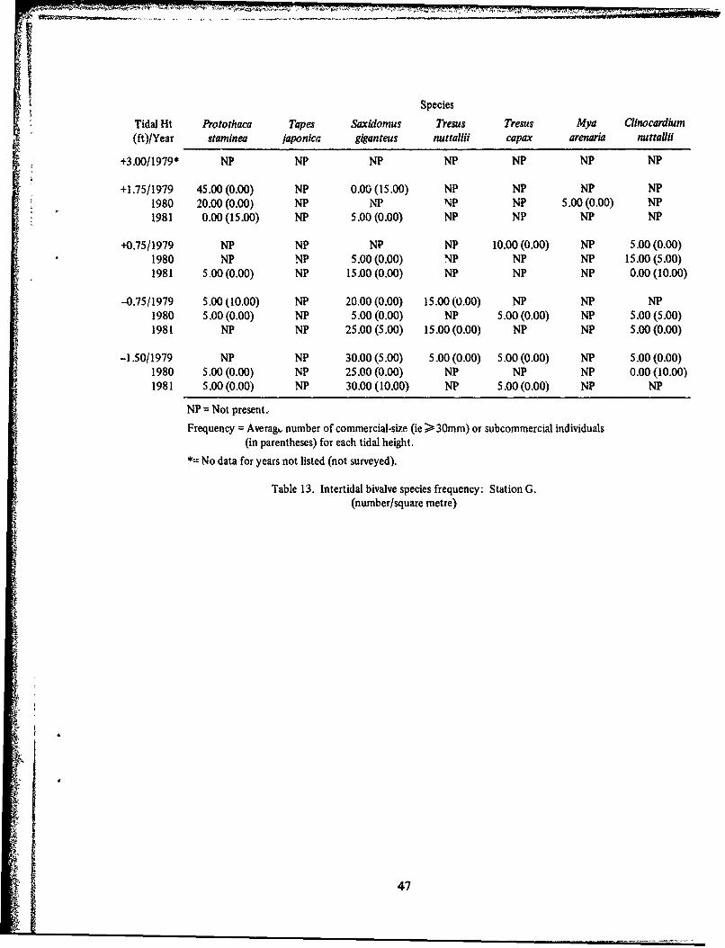
NP = Not present.

Frequency = Averag.. number of commercial-size (ie > 30mm) or subcommercial individuals(in parentheses) for each tidal height.

* No data for years not listed (not surveyed).

Table 13. Intertidal bivalve species frequency: Station G.(number/square metre)

47

Species

Tidal Ht Protothaca Tapes Saxidontus Tresus Tresus Mya Clinocardium(ft)/Year staininea japonica giganteus nuttallfi capax arenaria nuttaliui

+4.50/1979 15.00 (45.00) 5.00(5.00) NP NP NP 0.00 (10.00) NP1980 5.00 (20.00) 0.00 (10.00) NP NP NP NP NP1981 5.00 (85.00) 0.00(5.00) NP NP NP 0.00(5.00) NP

+2.50/1979 5.00 (50.00) NP 10.00 (30.00) NP NP NP 0.00(5.00)1980 10.00 (15.00) NP NP NP NP NP NP1981 10.00 (5.00) NP 20.00 (5.00) NP NP NP 5.00 (5.00)

+1.60/1979 0.00 (25.00) NP 5.00 (0.00) NP NP NP 0.00 (5.00)1980 10.00 (15.00) NP NP NP NP NP NP1981 0.00(5.00) NP 5.00(0.00) NP NP NP 0.00(5.00)

0.00/1979 0.00 (65.00) NP 0.00 (60.00) NP NP NP 5.00(0.00)1980 0.00 (15 00) NP NP NP 5.00 (0.00) NP 0.00 (20.00)1981 0.00 (5.00) NP NP NP NP NP 0.00 (5.00)

-1.60/1979 5.00 (0.00) NP 0.00 (5.00) NP NP NP NP1980 NP NP NP NP NP NP 0.00 (20.00)1981 NP NP NP NP 0.00 (5.00) NP NP

NP = Not present.

Frequency = Average number of commercial-size (ie > 30mm) or subcommercial individuals(in parentheses) for each tidal height.,

Table i4. Intertidal bivalve species frequency. Station J.(number/square metre)

Species

Tidal Ht Protothaca Tapes Saxidomus Tresus Tresus Mya Clinocardium(ft)/Year staminea japonica giganteus nuttaliji capax arenaria nuttallil

+3.50/1979* 15.00 (10.00) NP 5.00 (10.00) NP NP 10.00 (0.00) NP

+2.50/1979* 15.00 (95.00) 0.00(5.00) 5.00 (25.00) NP NP NP 0.00(5.00)

0.00/1979* 0.00 (15.00) NP 0.00 (15.00) NP NP NP 15.00 (20.00)

-1.00/1979* 0.00 (5.00) NP NP NP NP NP 5.00 (5.00)

NP = Not present.,

Frequency = Average number of commercial-size (ie > 30mm) or subcolmercial individuals(in parentheses) for -ach tidal height.

* = No data for years not listed (not su. . yed).

Station surveyed in 1979 only.

Table 15, Intertidal 1-zvalve species frequency: Station M.(number/square metre)

48

A comprehensive data base for intertidal bivalve populations along SUBASE Bangorhas been established through 11 surveys during the past eight years (1973-1981). These ex-tensive baseline data are necessary for detecting and evaluating potentially abnormal changesin bivalve populations, should they occur. Since 1973, natural fluctuations in bivalve popu-lations adjacent to SUBASE Bangor have been observed.

Station A

Intertidal bivalve samples were collected at Station A between +2.5- and -1.5-foottidal heights during 1979, 1980 and 1981 surveys. This off-base station is representative ofa typical intertidal beach area along northern Hood Canal (figure 2). A moderately steepbeach slope (!: 11 gradient) consisting of rocks and cobbles with interstitial pea gravel in theupper intertidal region is covered by scattered barnacles and mussels in the mid-intertidalregion (about +5.0-foot level). A well-developed oyster zone (at +3.5- to +1.0-foot levels)is present. At about the zero tidal level the substratum becomes fine sand and mud coveredby an eelgrass (Zostera marina) bed which extends subtidally to a depth of about 8 metres(figure 7). This exposed beach is subjected to moderate wave and wind action throughoutthe year.

V During the 1979 intertidal survey at station A,Protothaca staminea (native littleneck

clams) were most abundant at the +1.25-foot to zero tidal level and Saxidomus giganteus(butter clams) were densest lower intertidally at about the -1.25-foot level (table 9). Stationcommercial bivalve biomass estimates were 1.42 kg/m 2 for native littleneck clams, 6.84kg/m 2 for butter clams, 1.02 kg/m 2 for Tresus capax (horseneck clams) and 0.24 kg/m 2 forClinocardium nuttallii (basket cockles)., Commercial size bivalves (> 30 mm in greatest di-mension) were represented by the following station percentages: 36.9% for native littlenecks,59.5% for butter clams, 2.4% for ,'orseneck clams and 1.2% for basket cockles during 1979sampling activities. Juvenile YOY size (< 10 mm) native littleneck clams, butter clams andbasket cockles represented 30%, 20% and 50% of the individuals collected for each species,respectively. These data indicate that recruitment is occurring and that a reproducing assem-blage of commercially import-,it bivalves is present at this station.

During the 1980 survey, native littlenecks were most prevalent at the +1.25-foottidal level. Butter clams and basket cockles were concentrated at the -0.5-foot level;' how-ever, these species were also collected within the +1.25- to -1.5-foot tidal region. Commercial-size bivalve biomass data were highest at this station during the 1980 survey for native little-neck clams (1.88 kg/m 2 ) and butter clams (11.41 kg/m 2 ). Commercial-size bivalves repre-sented the following percentages during 1980 sampling activities-' 32.5% for native littleneckclams, 62.6% for butter clams, 1.6% for horseneck clams and 3.3% for Mya arenaria (easternsoftshell clams)., Recruitment was high for basket cockles (100% of individuals collectedwere < 10 mm) and less for native littleneck clams and butter clams, 17% and 4%,respectively.

Sclam During the 1981 intertidal bivalve survey, both native littleneck clams and butterSclams were most concentrated at the zero tidal level. Biomass estimates were somewhat re-

duced from the previous two years for native littleneck clams at 0.78 kg/m 2 and butterclams at 3.44 kg/m 2 . Butter clams again represented 60% of the commercial-size bivalves

49

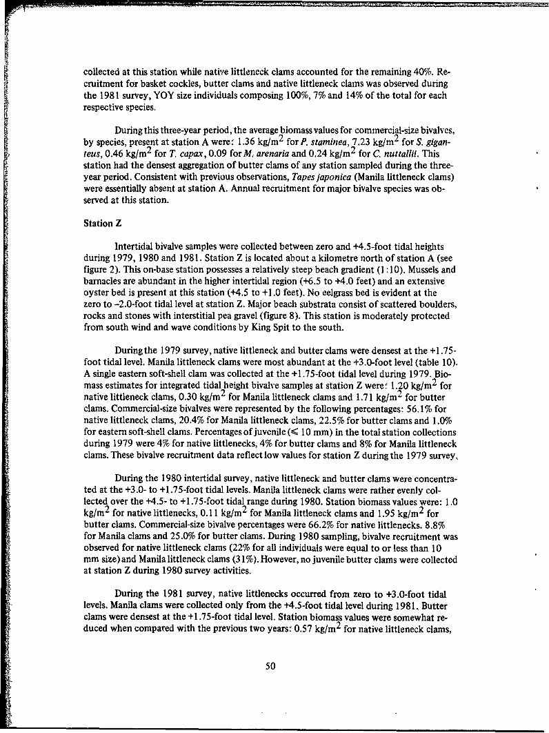
collected at this station while native littleneck clams accounted for the remaining 40%. Re-cruitment for basket cockles, butter clams and native littleneck clams was observed duringthe 1981 survey, YOY size individuals composing 100%, 7% and 14% of the total for eachrespective species.

During this three-year period, the average biomass values for commercial-size bivalves,by species, present at station A were* 1.36 kg/m 2 for P. staminea, 7.23 kg/m 2 for S. gigan-teus, 0.46 kg/m 2 for T. capax, 0.09 forM., arenaria and 0.24 kg/m 2 for C. nuttallii. This

station had the densest aggregation of butter clams of any station sampled during the three-year period. Consistent with previous observations, Tapes japonica (Manila littleneck clams)were essentially absent at station A. Annual recruitment for major bivalve species was ob-served at this station.

Station Z

Intertidal bivalve samples were collected between zero and +4.5-foot tidal heightsduring 1979, 1980 and 1981. Station Z is located about a kilometre north of station A (seefigure 2). This on-base station possesses a relatively steep beach gradient (1:10). Mussels andbarnacles are abundant in the higher intertidal region (+6.5 to +4.0 feet) and an extensiveoyster bed is present at this station (+4.5 to +1.0 feet). No eelgrass bed is evident at thezero to -2.0-foot tidal level at station Z. Major beach substrata consist of scattered boulders,rocks and stones with interstitial pea gravel (figure 8). This station is moderately protectedfrom south wind and wave conditions by King Spit to the south.

During the 1979 survey, native littleneck and butter clams were densest at the +1.75-foot tidal level. Manila littleneck clams were most abundant at the +3.0-foot level (table 10).A single eastern soft-shell clam was collected at the +1.75-foot tidal level during 1979. Bio-mass estimates for integrated tidal height bivalve samples at station Z were:. 1.20 kg/m 2 fornative littleneck clams, 0.30 kg/m 2 for Manila littleneck clams and 1.71 kg/m 2 for butterclams. Commercial-size bivalves were represented by the following percentages: 56.1% fornative littleneck clams, 20.4% for Manila littleneck clams, 22.5% for butter clams and 1.0%for eastern soft-shell clams. Percentages of juvenile (< 10 mm) in the total station collectionsduring 1979 were 4% for native littlenecks, 4% for butter clams and 8% for Manila littleneckclams. These bivalve recruitment data reflect low values for station Z during the 1979 survey.,

During the 1980 intertidal survey, native littleneck and butter clams were concentra-ted at the +3.0- to +1.75-foot tidal levels. Manila littleneck clams were rather evenly col-lected over the +4.5- to +1.75-foot tidal range during 1980. Station biomass values were: 1.0kg/m 2 for native littlenecks, 0.11 kg/m 2 for Manila littleneck clams and 1.95 kg/m 2 forbutter clams. Commercial-size bivalve percentages were 66.2% for native littlenecks. 8.8%for Manila clams and 25.0% for butter clams. During 1980 sampling, bivalve recruitment wasobserved for native littleneck clams (22% for all individuals were equal to or less than 10mm size) and Manila littleneck clams (31%). However, no juvenile butter clams were collectedat station Z during 1980 survey activities.

During the 1981 survey, native littlenecks occurred from zero to +3.0-foot tidallevels. Manila clams were collected only from the +4.5-foot tidal level during 1981. Butterclams were densest at the +1.75-foot tidal level. Station biomass values were somewhat re-duced when compared with the previous two years: 0.57 kg/m 2 for native littleneck clams,

50

0.02 kg/m 2 for Manila clams and 1.28 kg/m 2 for butter clams. Species percentages ofcommercial-size bivalves for 1981 samples were:., 62.9% for native littlenecks, 2.9% forManila clams and 34.2% for butter clams. Juvenile native littleneck and butter clams eachrepresented 13% of total individuals for each species. No Manila littleneck clam juveniles (< 10mm) were collected during the 1981 survey at station Z.

During 1979, 1980 and 1981 surveys the average biomass values for commercial-sizebivalves at station Z moere: 0.97 kg/m 2 for P. staminea, 0. 14 kg/m 2 for T. japonica and 1.65kg/m 2 for S. giganteus. This station ranks fifth out of seven during the three-year periodwith respect to commercial clam biomass. Recruitment of major bivalve species was low tosporadic during this period.

Station C

Intertidal bivalve samples were collected between zero and +5.5-foot tidal heights atstation C during 1979, 1980 and 1981 surveys. Station C is located in Carlson Covc betweenKB Pier and the New Service Pier (see figure 2). This station was potentially vulnerable toimpacts from construction activities at NSP during this sampling period. The measuredbeach gradient at this station is 1:9.73, the steepest gradient of all seven intertidal samplingbeaches along the SUBASE Bangor waterfront area (figure 9). The upper intertidal region atstation C consists of cobbles and stones with scattered boulders. An underlying layer of in-terstitial sand and pea gravel is present down to the +2.5-foot tidal level. Rocks and inter-stitial sand compose the substratum in mid and lower intertidal regions at this station. Scat-tered eelgrass is evident at the lowest tidal levels. This naturally sheltered cove became evenmore protected from wind and wave after the New Service Pier was built in 1981.

During the 1979 intertidal survey, native littleneck clams were most concentratedat the +2.5-foot tidal level. Butter clams were collected from zero to +2.5-foot tidal heightsand the densest concentration occurred at the +2.5-foot level (table 11). Most Manila clamswere collected from the +3.75-foot tidal level. Several juvenile eastern soft-shell clams werecollected at the +2.5-foot level during 1979. Station biomass estimates for commercial-sizebivalves wbre: 1.42 kg/m2 for native littleneck clams, 0.01 kg/m 2 for Manila clams, 2.56kg/m 2 for butter clams and 0.02 kg/m 2 for eastern soft-shell clams. Percentages of

commercial-size clams, by species, collected in 1979 at station C were: 66.7% for native little-neck clams, 1.1% for Manila littleneck clams, 31.1% for butter clams and 1.1% for easternsoft-shell clams. Juvenile commercial species recruitment was represented by 10% of nativelittlenecks, 50% of Manila clams and 7% of butter clams.

In 1980, native littleneck clams were concentrated again at the +2.5-foot tidal levelat station C. Manila clams were collected in equal abundance from +2.5- and +3.75-foottidal levels. Butter clams were concentrated at the +1.0-foot tidal height. Biomass estimatesfor commercial species at station C in 1980 were: 1.85 kg/m 2 for native littleneck clams,0.1 kg/m 2 for Manila clams and 2.69 kg/m 2 for butter clams. A single eastern soft-shell clamwas collected at +3.75-foot tidal level. Percentages of commercial-size bivalves collected dur-ing 1980 were: 71.1%, 5.2%, 22.7% and 1.0% for native littleneck clams, Manila clams,

51

L

butter clams and eastern soft-shell clams, respectively. Commercial clam species recruitmentwas represented by the following percentages of total individuals for each species: 11% fornative littlenecks, 13% for Manila clams and 8% for butter clams during 1980 collections.

During the 1981 intertidal survey, native littleneck clams were again most numerousat the +2.5-foot tidal level. No Manila clams were collected from this station in 1981. Butterclams were most concentrated at the zero tidal level; however, this species was present in

nearly equal abundance from +2.5 feet down to the zero tidal level. Station biomass esti-mates for commercial bivalves were., 0.88 kg/m 2 For native littleneck clams and 4.11 kg/rn 2

for butter clams. This value was the highest biomass estimate for butter clams during the1981 survey at all stations. Native littleneck clams represented 60% and butter clams 40% ofthe total bivalve individual abundance during 1981 sampling at station C. Juvenile bivalves(< 10 mm) recruitment data were highest at station C during 1981 sampling, with nativelittleneck clams representing 17% and butter clam juveniles representing 10% of the indivi-duals collected from each respective species.

Three-year mean biomass values at station C were: 1.38 kg/m 2 for native littleneckclams, 0. 1 kg/m 2 for Manila clams, 3.12 kg/m 2 for butter clams and 0.02 kg/m 2 for easternsoft-shell clams. This station has consistently produced an abundance of commercially im-portant bivalves. Even with the New Service Pier construction during 1979, 1980 and 1981,station C ranks only behind station A in total bivalve biomass (station averages used for corn-parison). A few Miarila and eastern soft-shell clams have been collected from this station. Nobasket cockles were collected during the three-year sampling period.

Station D

Intertidal bivalve samples were collected between +6.25- and -2.25-foot tidal levelsat station D during 1979, 1980 and 1981 surveys. As previously mentioned in the introduc-tion to this report, station D was established in 1979 to replace station E. Station D is locatedon the southern Devil's Hole delta region (see figure 2) between KB Pier and the Delta Com,-plex Facility. This transect extends from the high tide berm line consisting of stones, peagravel and shell debris down to zero tidal level at about the 125-metre mark along the tran-sect line (figure 10). The gently sloping beach gradient, measured from +6.5-foot tidal heightdown to -2.5-foot tidal height, is 1:45, Substratum a'-ng the mid-intertidal region consistsof sand and pea gravel. Below zero tidal level, fime sand and eelgrass patches are present. Awell-developed eelgrass bed begins at 130 metres along the transect line. This station is rela-tively sheltered from southerly wind and wave action. Station D (along with station G) isnear the primary center of Trident construction activities, the Delta Complex Facility.,

During the 1979 intertidal survey, native littleneck clams were collected from +5.0-to -2.25-foot tidal levels (table 12). Tapes japonica (Manila clams) were concentrated at the+6.25-foot tidal level during the 1979 sample collections. Butter clam concentrations weredensest at the +1.0-foot level; however, commercially sigrnificant sample digs were presentfrom -2.25- to +5.0-foot tidal levels. Eastern soft-shell clams were collected from +6.25-to +1.0-foot tidal levels, being most concentrated at the upper intertidal regions. Basketcockles were most numerous at the +2.0-foot tidal level. Biomass values for combined sam-ple sites at station D during the 1979 survey were., 0.62 kg/m 2 for native littlenecks, 0.05kg/m 2 for Manila clams, 1.78 kg/m 2 for butter clams, 0.07 kg/m 2 for eastern soft-shellclams and 0.18 kg/m 2 for basket cockles. Bival ,, percentages observed in 1979 samples

52

yielded the following composition by species: 3.6% for native littleneck clams, 3.2% forManila clams, 51.6% for butter clams, 5.4% for eastern soft-shel' clams and 3.2% for basketcockles Juvenile YOY bivalve recruitment data from 1979 collections (percentages, byspecies, composed of individuals I 1Omm in maximum dimension) were.- 71% for nativelittleneck clams, 35% for Manila littleneck clams and 64% for butter clams.

During the 1980 intertidal survey, native littleneck clams were densest at the +2.8-foot tidal level. Manila clams were concentrated at the +5.0-foot tidal level. Butter clamswere quite evenly distributed from +5.0- to -2.25-foot tidal levels during the 1980 sam-pling period. Most juvenile butter clams (Saxidomus giganteus) less than 30 mm were col-lected at the +2.0-foot tidal height. A few eastern soft-shell clams were collected from +5.0-and +1.0-foot tidal levels. Basket cockles were most numerous in -arunles at the zero tidallevel during 1980. Station bivalve biomass estimates were:' 0.74 kg/m' for native littleneckclams, 0.15 kg/m 2 for Manila clams, 2 01 kg/m 2 for butter clams, 0.13 kg/m 2 for easternsoft-shell clams and 0.15 kg/m 2 for basket cockles. During the 1980 survey the followingpercent composition data were collected for commercial-size bivalve species: 38.5% for nativelittleneck clams, 18.8% for Manila clams, 36.4% for butter clams, 2.1% for eastern soft-shellclams and 4.2% for basket cockles. Percentages ofjuven-le commercially important bivalves(< 10 mm) when compared with adults of the same species were.: 24% for native littleneckclams, 5% for Manila clams,, 15% for butter clams and 8% for basket cockles. Recruitmentof commercially important YOY bivalves is again evident from these data.

During the 1981 intertidal survey, native littleneck clams were densest at the +1.0-foot tidal level. Manila clams were concentrated high intertidally at +5.0 feet. Butter clamswere evenly distributed (about 50 individuals/square metre) from +2.0- to -2.25-foot tidallevels. Tresus capax (horseneck clams) were collected at station D during 1981 at the -2.25-foot tidal level. Eastern soft-shell clams were present at +5.0- and +2.0-foot tidal levels.Basket cockles were present at the zero tidal level. Combined station bivalve biomass datafor 1981 estimates were. 0.57 kg/m 2 for native littleneck clams, 0.15 kg/m 2 for Manilaclams, 2.28 kg/m 2 for butter clams, 0.27 kg/m 2 for horseneck clams, 0.01 kg/m 2 for easternsoft-shell clams and 0.04 kg/m 2 for basket cockles. Percentages of numerical abundance byspecies were. 26.7% for native littleneck clams, 25.5% for Manila clams, 44.2% for butterclams, 1.2% for horseneck clams, 1.2% for eastern soft-shell clams and 1.2% for basket coc-kles. Recruitment for native littlenecks (40% of all individuals were < 10 mm) and butterclams (29%) was observed during the 1981 intertidal survey at station D.

During the 1979, 1980 and 1981 intertidal surveys, the mean commercial bivalvebiomass values by species were: 0.64 kg/m 2 for native littleneck clams, 0.12 for kg/m 2 forManila littleneck clams, 2.01 kg/m 2 for butter clams, 0.07 kg/m 2 for T. capax, 0.07 kg/m2

for eastern soft-shell clams and 0.12 kg/mr2 for basket cockles. This station ranked fourth inoverall clam biomass when compared with six other sampling stations. Species abundanceand distribution for bivalves are considered more representative of the entire delta regionthan were data previously collected at station E. Excellent recruitment of commercial bi-valve species occurred durin,, the three-year period.

Station G

Intertidal bivalve samples were collected between +1.75- and -1.5-foot tidal levelsduring the period 1979, 1980 and 1981 at station Gt -,e figure 2). A moderately steep beach

53

giadient (1: 12) exists at this station fro& +6.0- to -2.0-foot tidal heights (figure 11). Theupper intertidal area at station G contains large boulders and nip-rap along the initial fivemetres of transe..t distance down to the +6.0-foot tidal level. Beyond this and extendingdown into the +1.0-foot tidal region, the substratum is composed of stones and pea gravelwith interstitial sand. Below +1.0 foot the substratum becomes a mud-sand mixture andeelgrass is present at about the zero tidal level. At about -3.0-foot tidal level a steep claybank (approximately 250 slope or 1:2 gradient) develops and continues to a depth of 10metres. During diving observations, this clay bank has been seen to support a population ofthe boring piddock clam (Zirphaea pilsbryi). Station G has been potentially impacted bywaterfront operations at Marginal Wharf for several decades and by additional constructionactivities at the Delta Complex during the past several years. This station is moderatelysheltered from wind and wave conditions.

During the 1979 intertidal survey, native littleneck clams were concentrated at the+1.75-foot tidal level at station G (table 13). Butter clams were densest at the -1.5-foot level.No Manila clams were present at this station. Both T. capax and T. nuttallii (horseneckclams) were commonly collected at station G at +0.75- to -1.5-foot tidal levels. Basket coc-kles were also collected from this tidal range. Biomass estimates for 1979 bivalve data at sta-tion G were: 0.52 kg/m 2 for native littleneck clams, 2.0 kg/m 2 for butter clams, 0.65 kg/m2for T. nuttallii and 0.26 kg/m 2 for T. capax, 0.87 kg/m 2 for eastern soft shell clams and0.20 kg/m 2 for basket cockles. Percent composition by species for commercial-size bivalveswere as follows:" 31.3% for native littleneck clams, 31.3% for butter clams, 12.5% for T,.nuttallii, 9.4% for T. capax, 9.4% for eastern soft-shell clams and 6.1% for basket cockles.Commercial bivalve species recruitment for individuals < 10 mm as expressed by percentageof juveniles was: 8% for iiative littlenecks, 29% for butter clams and 30% for basket cocklescollected at station G during the 1979 survey.

During the 1980 intertidal survey, again, native littlenecks were most numerous atthe +1.75-foot tidal level. Butter clams, while never abundant at this station, were densest at-1.5-foot tidal height. A single T. capax was collected at -0.75-foot tidal height during the1980 survey. Additionally, a single soft-shell clam was collected at the +1.75-foot tidal level.Basket cockles were concentrated at the +0.75-foot level. Station bivalve biomass estimatesfor commercial-size bivalves at station G were:., 0.31 kg/m 2 for native littleneck clams, 0.98kg/m 2 for butter clams, 0.09 kg/m 2 for T. capax, 0.03 kg/m 2 for eastern soft-shell clams,and 0.52 kg/m 2 for basket cockles. Percent composition by species was: 31.5% for nativelittlenecks. 36.8% for butter clams, 5.2% for T. capax, 5.2% for eastern soft-shells and 21.3%for basket cockles. No recruitment was observed for native littleneck clams in 1980 at thisstation. Butter clams and basket cockles were represented by 12.5% and 37.5% of total indi-viduals < 10 mm for each respective species.

During the 1981 intertidal survey at station G, native littleneck clams were infre-

quently collected. Specimens of this species were present at +0.75- and -1.5-foot tidal levels.Butter clams were most numerous at -1.5-foot tidal height. Again, a single specimen of 7T.capax was collected from -1.5-foot tidal level. Basket cockles were sparsely distributed andonly collected at the +0.75-foot tidal height. Station biomass estimates for 1981 commercialbivalve data were:. 0.10 kg/m 2 for native littleneck clams, 3.09 kg/m 2 for butter clams, 0.65kg/m 2 for T., nuttallii, 0. 11 kg/m 2 for T. capax and 0.44 kg/m 2 for basket cockles. Percentcomposition based on number of commercial-size bivalves for 1981 collections were:. 8.3%for native littleneck clams, 62.5% for butter clams, 12.5% for T. nuttallii, 4.2% for T. capax

54

and 12.5% for basket cockles. Twenty percent of the native littleneck clams collected atstation G during 1981 were < 10 mm in size. No recruitment was evident for other commer-cial bivalve species in 1981 samples at this station.

During the period 1979, 1980 and 1981 the following average biomass data forcommercial-size bivalves were collected at station G:, 0.22 kg/m 2 for native littleneck clams,2.02 kg/m 2 for butter clams, 0.43 kg/m 2 for T.. nuttallii, 0.15 kg/m 2 for T., capax, 0.30kg/m 2 for eastern soft-shell clams and 0.39 kg/m 2 for basket cockles. This station ranksthird in terms of total bivalve biomass during the three-year period. Moderate recruitment ofYOY native littleneck clams, butter clams and basket cockles occurred at station G during1979, 1980 and 1981.

Station J

Intertidal bivalve samples were collected between +4.5- and -1.4-foot tidal heightsat station J during 1979,1980 and 1981 surveys. As previously discussed in the introductionsection of the report, station J was established to replace station K in 1979. Station J islocated on the northern side of Cattail delta (see figure 2). A beach gradient of 1:37 wasmeasured from +5.5- to -1.5-foot tidal levels at this station (figure 12). The upper inter-tidal region consists of stones and rocks covering sand and pea gravel. Mussels and barnaclesare abundant at the +5.0-foot tidal height at this station. A well-developed oyster bed is pre-sent in the +4.0- to +1.0-foot tidal zone. Substratum along the mid-intertidal region consistsof coarse sand and scattered rocks. Below zero tidal level, eelgrass and fine gray sand com-pose the primary substratum. This station is sheltered from southerly wind and wave condi-tions, but openly exposed to weather from the north.

During the 1979 intertidal survey, native littleneck clams were concentrated at the+4.5- to +2.5-foot tidal region along the transect (table. 14). Manila clams were present at+4.5-foot tidal level. Butter clams were collected from 1 42.5- to -1.6-foot tidal levels, butwere most abundar.t at the +2.5-foot tidal level. Eastern soft-shell clams were collected onlyat the +4.5-foot tidal height. Basket cockles occurred from +2.5- to -1.6-foot tidal regions.Commercial-size bivalve biomass estimates at station J during the 1979 survey were: 0.05kg/m 2 for native littleneck clams, 0.01 kg/m 2 for Manila clams, 0.30 kg/m 2 for butter clamsand 0.02 kg/m 2 for basket cockles. Perc.nt composition for commercial-size bivalves byspecies were: 44.4% for native littleneck clams, 11.1% for Manila clams, 33.4% for butterclams and 11. 1% for basket cockles. Juvenile commercial bivalve species (•< 10 mm in size)represented the following percentages of all individuals for that species: 74% for native little-neck clams, 83% for butter clams and 50% for basket cockles during the 1979 survey.,

During the 1980 intertidal survey at station J, native littleneck clams were evenlydistributed from the +4.5- to +1.6-foot tidal region. Several juvenile Manila clams were col-lected from the +4.5-foot tidal level. No butter clams were collected at station J in 1980.Tresus capax were present at the zero tidal level, as were the densest concentrations of bas-ket cockles. Station biomass estimates during the 1980 survey were: 0.01 kg/m 2 for nativelittleneck clams, 0.57 kg/m 2 for 7". capax and 0.09 kg/m 2 for basket cockles. Percent com-position by species for commercial-size bivalves at ths station were. 60% native littlenecks,20% T, capax and 29% basket cockles during the 1980 survey. Percentage data for YOYjuvenile bivalves (< 10 mm in size) were: 70% for native littlenecks, 50% for Manila clams,

55

and 78% for basket cockles. These data indicate excellent recruitment for commercial bi-valve species at station J, but conditions appear less than adequate for reasonable bivalvegrowth and survival.

During t.U, 1981 intertidal bivalve survey, native littleneck, Manila and eastern soft-shell claws were most concentrated at the +4.5-foot tidal level. Butter clams were mostabundant at the +2.5-foot level. Tresus capax were collected at the -1.6-foot tidal heightalong the transect. Basket cockles were distributed from zero tidal level to +2.5 feet inter-tidally.. Station bivalve biomass estimates for commercial-size clams by species at station Jdurinm 1981 were: 0.09 kg/m 2 for native littlenecks, 0.52 kg/m 2 for butter clams and 0.13kg/mr for basket cockles. Percent composition by species for commercial-size clams were:'33.3% for native littleneck clams, 55.6% for butter clams and 11.1% for basket cockles dur-ing the 1981 survey. Juvenile commercial clam species represented 17% of native littleneckclams, 14% of bucter clams and no basket cockles at station J during 1981.

Du-ing this three-year s~inpling period, the average biomass for commercial-size bi-vwlves by s.ccies at station J were., 0.05 kg/m2 for native littleneck clams, 0.27 kg/m 2 for

utter claw'", 0.02 kg/in2 for :. capax and 9.08 ktm2 for basket cockles. Station J ranks

last ,ut ot seven intenidal saw.A,-!U-1 stations cr, t!-e basis of overall clam biomass. Conversely,bivalve rac-citrnent is highest at tlis station. Again, a consistent pattern for bivalve data (asreported at Station K previously, reference 3) indicates that conditions for bivalve growthand survival at station J are extremely poor.

Station M

This northern off-base control station was sampled only during the 1979 intertidalsurvey. As discussed previously in the introduction to this report, station M was establishedto replace station L,. but did not provide representative data on commercially-significant bi-valves. Station M was located approximately two kilometres north of station I (refer tofigure 2). Intertidal bivalve samples were collected at station M between the +3.5- and -1.0-foot tidal levels. A beach gradient of 1:28 was measured for this intertidal range (figure 13).High intertidal substratum consisted of sand and pea gravel, with overlying scattered stonesand boulders. At about a +4.0-foot tidal height, sand covered rocks and stones. Patchy eel-grass and ulvoids were present at zero tidal level and developed into a dense eelgrass bedbelow the -0.5-font tidal level on the transect axis. Substratum in the eelgrass bed was finegray sand. This staion was moderately exposed to wind and wave action during mostseasons.

During the 1979 intertidal survey, native littleneck and butter clams were concen-trated at the +2.5-foot tidal level (table 15). A single Manila clam was also sampled at thisintertidal height. Eastern soft-shell clams occurred only at the +3.5-foot tidal height. Basketcockles were densest at the zero tidal region. Station biomass estimates for commercial bi-valves at station M by species were: 0.19 kg/m 2 for native littleneck clams, 0.29 kg/m 2 forbutter clams, 0.07 kg/m 2 for eastern soft-shell clams and 0.85 kg/m 2 for basket cockles.Commercial-size clams were represented by the following percentages: 42.9% for nativelittlenecks, 14.3% for butter clams, 14.3% for eastern soft-shell clams and 28.5% for basketcockles. Only 14 commercial-size individiual bivalve specimens (representing four species)

56

were collected at station M duiing the 1979 intertidal sampling activities. Seventy-five per-cent of all native littleneck clams and butter clams were < 10 mm in size. This station clear-ly was not representative of a commercially-significant clamming beach. Intertidal samplingat station M was terminated after the 1979 survey.

Intertidal bivalve surveys conducted at SUBASE Bangor during 1979, 1980 and 1981further describe the abundance and distribution of important molluscan species along HoodCanal shoreline areas. Samples were collected from regions of commercially and recreational-ly significant bivalve populations to estimate density, standing crop (biomass) and recruit-ment of important species. Methods and locations of intertidal sampling activities duringthis period are comparable with previous NOSC Trident surveys.

Table 16 summarizes mean bivalve density, by species, for each station during thisthree-year sampling period. Species ranked in decreasing order of integrated mean densitiesare: Protothaca staminea, Saxidomus giganteus, Tapes japonica, Clinocardium nuttallii, !dyaarenaria, Tresus capax and T., nuttalili. Stations ranked in decreasing order of total clam den-sity, where all commercial species are combined are D, Z, C, A, M, J and G. Buttur clamsand native littleneck clams were numerically dominant at all stations sampled during thisperiod. Generally, bivalve populations were denser at southern stations (A, Z C and D) thannorthern stations (G, J and M). Total biomass of commercial-size clams collected during1979, 1980 and 1981 art apportioned among all stations as follows: butter clams, 65%;native littleneck clams, 19%; basket cockles, 7%; Tresus capax, 4%;' Tresus nuttallii, 2%;eastern soft-shell clams, 2% and Manila littleneck clams, 1%. Biomass of commercial-size bi-valves was shared among stations, from highest to lowest values, as follows: A, C, G. D, Z, Mand J.

Commercial bivalve species recruitment data collected during 1979, 1980 and 1981surveys are summarized in table 17, Stations D and J had the highest percentages of smallbivalves (< 10 mm), and, thus, presumably the highest recruitment potential for butter andnative littleneck clams. During the 1979 survey, basket cockle recruitment was greatest atstations A, J and G. The recruitment level of YOY juvenile bivalves (< 10 mm) was observedto be generally independent of the adult clam population size at a given station. Stadi, nshaving a gently sloping beach gradient (often delta regions) consistently exhibited greaterbivalve recruitment, while they often possessed a less dense adult bivalve populatien, Condi-tions responsible for heavy settlement of juvenile bivalves are apparently unrelated to theenvironmental requirements necessary for sustained growth and survival.

Total mean density of commercial-size bivalves (#/square metre) and biomass (kg/square metre) are compared in table 18 from deta collected during a six-year period (1976-1981). Previously utilized sampling stations (E, K, L and M) are included for comparativepurposes in this summary. Again, a consistent pattern of higher bivalve density and greaterbiomass at southern stations is apparent. Stations A, C, Z and D continue to provide com-mercially significant densities and weights of clams along SUBASE Bangor. Eighty-fivepercent of the commercial bivalve biomass collected during the six-year period was attribu-table to these four stations. Stations A and C have remarkably similar overall bivalve produc-tivity characteristics. While beach gradient and substratum composition are similar at these

57

Species

Protothaca Tapes Saxidomus Tresus capax* Mya ClinocardiumStation Size Staminea Japonica giganteus or T., nuttalfii arenaria nuttafii

s • s s z s s s s

A comm 36.25(15.16) NP 63.33(33.76) 1.67(1.44)* 1.67(2.89) 0.42(0.72)subc 17.08(1.91) 0.42(0.72) 83.33(5.91) NP NP 9.75(10.39)

Z comm 50.83(21.2) 11.25(12.3) 21.25(6.25) NP 0.42(0.72) NPsubc 28.75(15.7) 36.25(40.5) 2.50(2.17) NP NP NP

C comm 69.58(18.3) 2.50(3.31) 31.67(3.61) NP 0.83(0.72) NPsubc 31.67(13.4) 6.67(8.51) 4.17(1.91) NP NP NP

D comm 32.33(,.08) 14.33(10.0) 40.00(6.24) 0.33(0.58)* 3.00(1.73) 2.67(1.53)subc 73.00(26.2) 13.33(11.0) 55.33(36.7) NP 1.67(2.08) 3.67(4.62)

G comm 8.22(5.75) NP 14.82(6.36) 3.33(2.97)* 1.85(2.21) 4.05(1.09)subc 2.38(2.18) NP 3.75(2.28) NP NP 2.62(2.51)

3 comm 4.03(0.87) 0.42(0.72) 3.10(3.84) 0.42(0.72)* NP 1.20(0.08)subc 31.16(13.2) 1.62(0.77) 8.66(13.12) NP 1.20(1.25) 4.91(4.41)

M** comm 8.57 NP 2.85 NP 2.86 5.71subc 34.29 1.43 14.29 NP NP 10.00

"*denotes Tresus capax."**station M was sampled only during 1979.

S= mean.s = standard deviation.comm = commercial-size individuals.subc = subcommercial-size individuals.

Table 16. Combined mean intertidal bivalve density data (number/square metre) collectedduring 1979, 1980 and 1981 surveys at SUBASE Bangor.

58

Species

Station/ Protothaca Tapes Saxidomus ClinocardiumYear staminea Japonica giganteus nuttallif

4i A/1979 140.00 (30.43) 0.00 (0.00)2 120.00 (19.35) 20.00 (50.00)1980 90.00 (16.67) NP 30.00 (3.61) 170.00 (100.00)1981 40.00 (14.29) NP 20.00 (7.41) 30.00 (100.00)

Z/1979 40.00 (4.40) 70.00 (8.33) 10.00 (4.00) NP1980 150.00 (2239) 90.00 (31.03• 0.00 (0.00)2 NP1981 40.00 (12.90) 0.00 (0.00) 20.00 (13.33) NP

C/1979 80.00 (9.76) 70.00 (50.00) 20.00 (6.67) NP1980 90.00 (10.59) 10.00 (12.50) 20.00 (8.33) NP1981 100.00 (17.24) NP 30.00 (10.00) NP

D/1979 990.00 (70.71) 60.00 (35.29) 930.00 (64.14) 0.00 (0.00)21980 220.00 (23.91) 20.00 (4.76) 90.00 (14.52) 10.00 (7.69)1981 340.00 (40.96) 0.00 (0.00)2 230.00 (29.11) 0.00 (0.00)2

G/1979 10.00 (8.33) NP 40.00 (28.57) 10.00 (50.00)1980 0.00 (0.00)2 NP 10.00 (12.50) 30.00 (37.50•1981 10.00 (20.00) NP 0.00(0.00) 0.00(0.00)

J/1979 310.00 (73.8 ) 0.00 (0.00)2 190.00 (86.36) 10.00 (50.00)1980 120.00 (70.59) 10.00 (50.00) NP 70.00 (77.78)1981 40.00 (17.39) 0.00 (0 .0 0 )p 10.00 (14.29) 0.00 (0.00)S

M/1979 210.00 (75.00) 0.00 (0.00)2 90.00 (75.00) 0.00 (0.00)2

NP = Not present.

1Number of juveniles (ie R < 10mm.), percentage of juveniles in parentheses.2 No recruitment evident; commercial-size individuals present,

Table 17., Commercial clam species recruitment (#/m2) (see footnote 1).

59

StationYear Measurement A Z C D E G J K L M

1976 D 158 78 144 NS 78 20 NS 27 5 NSB 5.5 5.4 4.5 3.3 1.4 0.3 0.5

1977 D 120 94 116 NS 98 30 NS 35 50 NSB 5.9 5.7 10.4 4.7 4.0 0.5 6.2

1978 D 180 76 164 NS 78 47 NS 42 NC NSB 9.9 3.4 10.8 6.3 2.4 0.5

1979 D 105 123 109 93 NS 46 9 NS NS 20B 10.9 3.2 4.0 2.8 3.4 0.4 1.4

1980 D 137 85 121 96 NS 24 6 NS NS NSB 11.9 3.1 4.7 3.2 1.9 0.2

1981 D 50 44 84 86 NS 34 10 NS NS NSB 4.2 1.9 5.0 3.3 4.4 0.7

NS = Not sampled.NC = No commercial.size bivalves collected.D = density.B = biomass.

Density = Z individuals w/ 2 > 30 mm(#digs containing commercial clam species)(0.1 m2 ) (1000)

i Biomass = 2 weights of clams w/ Q>mm

(# digs containing commercial clam speciesX0.1 m2 ) (1000)Note:. all commercial-size species data are combined.,

Table 18. Commercial bivalve density (#/m 2 ) and biomass (kg/m 2 ) data collected at all SUBASE Bangorsampling stations during the period 1976-1981.

I6

• 60

two stations, the proximity of station C to heavily utilized service piers demonstrates thelack of measurable adverse impact on bivalve populations along SUBASE Bangor.

We also evaluated the occurrence of commercial-size bivalves in relation to meantidal height using data from seven stations sampled during 1979, 1980 and 1981 surveys.Commercial dig frequency results are summarized in table 19. Frequency values representthe percent of sample digs which are commercially significant (i.e. bivalve wet biomass values> 277 grams/0.1 square metre of 2.77 grams/square metre) at each station. Mean tidalheights describe hypothetical intertidal levels where the densest concentrations of bivalvesoccur. These two statistics are useful for between-station comparisons of bivalve distribution.Stations C and Z exhibit higher commercial bivalve concentrations at upper tidal heights.The pattern is attributed to an abundance of littleneck clams which represent greater thansixty percent of commercial-size clams at these two stations. As shown in figure 4, nativelittleneck clams occur higher intertidally than butter clams. At stations A, D and G, butterclams represented the most common commercial-size species collected.

Oyster frequency data collected during intertidal transect sampling are presented intable 20. Oysters occurred from +6.25- to +1.0-foot tidal levels during this period. The great-est oyster densities were recorded at stations C and Z, between +4.5- and +1.75-foot tidalheights. A comprehensive oyster mapping survey performed by SUBASE Bangor fish andwildlife personnel is summarized in appendix C. These data generally agree with previoussurveys (ref 3).

Eelgrass (Zostera marina) beds along SUBASE Bangor were described previously (ref3). Comparable eelgrass data for the three new sampling stations, D, J and M, were takenduring the 1979 survey and are summarized in table 21. Previous evaluations of eelgrassstanding crop (biomass) and turion densities at SUBASE Bangor stations have described highvariability in these data. Based upon previous recommendations (ref 3), eelgrass samplingwas deleted from survey activities after the 1979 field efforts.

CONCLUSIONS

1. During 1979, 1980 and 1981 surveys, intertidal bivalve populations along SUBASEBangor and adjacent shoreline regions were numerically dominated by the following speciesin decreasing order of abundance,, native littleneck clams, butter clams, Manila littleneckclams, basket cockles, eastern soft-shell clams and horseneck clams.

2. The total bivalve biomass (kg/square metre) was distributed as follows:, butterclams, native littleneck clams, basket cockles, horseneck clams, eastern soft-shell clams andManila littleneck clams.

3. The relative importance of survey stations in terms of biomass of commercial-sizebivalves, ranked in decreasing order, was: A, C. G, D, Z, M and J.

4. Recruitment during the three-year period was documented for native littleneckclams and butter clams at all stations. Recruitment levels were highest at stations D and Jfor these two species. Stations A and J showed significant basket cockle recruitment, es-pecially during the 1980 survey. The recruitment of juvenile bivalves was apparently

____61

Station

Year A C D G J M Z

1979 0.75 0.63 0.50 0.38 0.00 0.00 0.63(-0.50 ±0.45) (+1.17 ±1.13) (+0.80 k..64) (-1.10 ±0.38) (NA) (NA) (+1.10 ±1.08)

1980 0.89 0.50 0.50 0.13* 0.13* NS 0.63(-0.23 ±+1.00) (+1.44 ±1.07) (+0.33 ±1.86) (-1.50)* (0.00)* (+1.16 ±1.18)

1981 0.50 0.63 0.50 0.63 0.10* NS 0.25(-0.25 ±0.29) (+1.20 ±1.25) (-0.20 ±1.79) (-0.70 ±0.84) (+2.00) (+1.50 ±-0.0)

Mean 0.71, (0.20) 0.59, (0.08) 0.50, (0.0) 0.38, (0.25) 0.08, (0.07) 0 0.50, (0.22)(Standarddeviation)

frequency dis commercial digs

# digs containing commercial clam species

Commercial dig = dig w/ Z weights of commercial.size individuals >277.0 g.

Mean tidal height index (ft) = 2; tidal heights of commercial digs

# of commercial digs*single commercial dig present.

Table 19. Commercial dig frequencies at SUBASE Bangor (1979, 1980 and 1981).(Mean tidal height ± standard deviation in parentheses).

62

Station

Tidal Ht(ft)/Year A C D G J M Z

+6.25/19791980 NS 70.00 (30.00)1981 NS NS

+5.25/1979 0.00 (280.00)1980 130.00 (20.00) 50.00 (40.00)1981 NS NS

+5.00/19791980 80.00 (0.00) 20.00 (20.00)1981 NP NS

+4.50/1979 45.00 (250.00)1980 200.00 (110.00) 40.00 (30.00)1981 90.00 (90.00) 80.00 (65.00)

+3.57/1979 50.00 (380.00)1980 226.67 (53.33)1981 260.00 (65.00)

+3.50/1979 NP1980 NS1981 NS

+3.00/1979 20.00 (90.00) 510.00 (455.00)1980 260.00 (30.00) NS 595.00 (280.00)1981 NS NS 450.00 (135.00)

+2.50/1979 NP 625.00 (535.00)1980 400.00 (45.00) 20.00 (0.00) NS 610.00 (190.00)1981 385.00 (35.00) 100.00 (25.00) NS NS

+2.00/1979 40.00 (45.00) 410.00 (260.00)1980 NP 170.00 (20.00) NP NS1981 15.00 (0.00) NS NP NS

+1.75/19791980 NP 15.00 (0.00) 375.00 (145.00)1981 NP NP 290.00 (35.00)

+1.25/19791980 NP1981 65.00 (20.00)

+1.00/19791980 15.00 (15.00) NP1981 NP NP

A C D G J M Z

NP = Not present.NS = Not surveyed.Frequency = mean number of individuals > 2" (mean number of individuals < 2" in parentheses).

Table 20. Oyster frequencies (number/square metre) present in quadrats during intertidaltransect surveys at SUBASE Bangor (1979, 1980 and 1981)

63

Density BiomassDistance across Densit 2 BiomaStation bed, m (percent*) turions/m g dry wt./m2

D 1(0) 910 172

23 (33) 875 97

46(66) 605 147

72(100) 135 60

J 1(0) 690 71

42(33) 525 88

84(66) 660 116

126(100) 210 71

M 1(0) 1740 103

19(33) 1580 100

60(66) 420 78

88 (100) 320 80

*percent distance across bed from upper (0%) side to deepest (100%) side.

Table 21. Eelgrass bed width, turion density and biomass data collectedduring July, 1979 at SUBASE Bangor.

64

'i • independent of the adult bivalve population at a given location. These data suggest thatconditions producing extensive larval release and settlement are unrelated to environmental

parameters which support increased growth and survival for commercial bivalve populationsadjacent to SUBASE Bangor.

S. Maximum densities of commercial-size bivalves along SUBASE Bangor shorelinesoccur between the +2.0- and -1.5-foot tidal levels.

6. The four southernmost sampling stations (A, Z, C and D) supported the greatestdensities and biomass of commercial-size bivalves along SUBASE Bangor.

7. Intertidal data collected during 1979, 1980 and 1981 demonstrate that commer-cially important bivalve populations are experiencing normal recruitment, growth and sur-vival adjacent to SUBASE Bangor. On-base construction and operational activities have not

produced detectable adverse impacts on the intertidal component of the marine ecosystem.

8. Commercially harvestable oyster beds along SUBASE Bangor represent a signifi-cant resource. A resource management plan has been developed (appendix Q.

65

HEAVY METAL SURVEYS

INTRODUCTION

Nearshore marine ecosystems respond to many natural and man-induced perturba-tions. Certain ecosystem component parameters can be used to detect and evaluate theseconditions. Indications of abnormal conditions are measurable with varying degrees of relia-bility. Ecosystem components such as sediments and selected organisms have been widelyused to evaluate the presence and effects of heavy metal contamination in nearshore marineenvironments (ref 34-51).

34 Alexander, GV and Young, DR, Trace Metals in Southern Californian Mussels, Marine Pollution Bulletin,vol 7, p 7.9, 1976

35Ayling, GM, Uptake of Cadmium, Zinc, Copper, Lead and Chromium in the Pacific Oyster, Crassostreagigas, Grown in Tamar River, Tasmania, Water Research, vol 8, p 729-738, 1974

36Bloon:, H, and Ayling, GM, Heavy Metals in Derwent Estuary, Environmental Geology, vol 2, p 3-22,1977

37Darracott, A, and Watling, W The Use of Molluscs to Monitor Cadmium Levels in Estuaries and CoastalMarine Environments, Trans Royal Society of South Africa, vol 41, p 325.338, 1975

38Emerson, RR, Soule, DF, and Oguri, M, Heavy Metal Concentrations in Marine Organisms and SedimentsCollected Near an Industrial Waste Outfall, Allan Hancock Foundation USC Seagrant Publ R402-76,p 1-15, 1976

39Frazier, JM, The Dynamics of Metals in the American Oyster, Crassostrea virginica. 1. Seasonal Effects,Chesapeake Science, vol 16, p 162-171, 1975

40Frazier, JM, The Dynamics of Metals in the American Oyster, Crassostrea virginica. 2. EnvironmentalEffects, Chesapeake Science, vol 17, p 188-197, 1976

4 1Goldberg, ED, et al, The Mussel Watch, Environmental Conservation, vol 5, p 101-125, 197842Hugget, RJ, Bender, ME, and Sloane, HD Utilizing Metal Concentration Relationships in the Eastern

Oyster (Crassostrea virginica) to Detect Heavy Metal Pollution, Water Research, vol 7, p 451-460, 197343Jenkins, DW, Biological Monitoring of Toxic Trace Metals. Biological Monitoring and Surveillance,

EPA-600/3-80.089, 215p, 198044Milins, DC, McCain, BB, Brown, DW, Sparks, AK, and Hodgins, HG, Chemical Contaminants and Biolo-

gical Abnormalities in Central and Southern Puget Sound, NOAA Tech Memorandum OMPA-2, MESAPuget Sound Project, 295p, 1980

4 5Miyahaa, S, Pollution of Sea Depending on the Heavy Metals and Oils:' Annual Variation of Mercury andCadmium in Seawater and Fundamental Properties of Floating Oil, Nagasaki University, Faculty ofFisheries Report, 15p, 1976

46phillips, DJH, Yim, WW-S, A Comparative Evaluation of Oysters, Mussels and Sediments as Indicators ofTrace Metals in Hong Kong Waters, Marine Ecology, vol 6, p 285-293, 1981

4 7Thompson, JAJ and Paton, DW Heavy Metals in Benthic Organisms from Point Grey Dumpsite,Vancouver, BC: a preliminary report, Pacific Marine Science Rept, 18p, 1978

48Topping, G, Heavy Metals in Fish from Scottish Waters, Aquaculture, vol 1, p 373-377, 197349Trefry, JH, and Presley, BJ, Heavy Metals in Sediments from San Antonio Bay and the Northwest Gulf

of Mexico, Environmental Geology, vol 1,283-294, 197650Windom, H, Stickney, R, Smith, R, White, D and Taylor, F, Arsenic, Cadmium, Copper, Mercury, and

Zinc in Some Species of North Atlantic Finfish, Journal Fisheries Research Board of Canada, vol 30,p 275-297, 1973

5 1Naval Undersea Center TP 457, Heavy Metal Contamination from Navy Ship Hulls, by S Yamamoto,JB Alcauskas, WH Shipman, RH Wade and RR Kenis, 34p, 1975

66

SUBASE Bangor environmental surveys have been designed to provide baseline dataon the presence of cadmium, chromi'um, copper, mercury, lead, tin and zinc in the environ-ment and ecosystems of adjacent areas in Hood Canal. Selected heavy metals were analyzedfrom sediments and certain tissue samples collected during the 1980 and 1981 surveys atSUBASE Bangor (figures 14 and 15). Such heavy metal monitoring can detect anomolouslevels of contaminants which may in turn indicate environmental stress.

Representative sampling areas were selected according to the following criteria.1) maximal operational fleet activity; 2) moderate support craft activity; or 3) no pier facili-ties or ship-related activity (control sites). These criteria were chosen to provide a range ofheavy metal content in sediments and organism tissues. A broad range of phyletic, trophicand habitat levels were also considered important in selecting specific organisms for tissueanalyses. Organisms selected for 1980 heavy metal analyses were: copper rockfish, Sebastescaurinus Richardson, 1845, red rock crab, Cancer productus, Randall, 1839; bay mussel,Mytilus edulis Linnaeus, 1758, and sea cucumber, Parastichopus californicus, Stimpson,1857. During 1981 sampling, sea cucumbers were deleted and replaced by the Pacific oyster,Crassostrea gigas (Thunberg, 1795). Oysters were chosen because they are 1) ubiquitouslydistributed along SUBASE Bangor. 2) readily collected, 3) widely used in heavy metalmon!toring, and 4) commercially important. Bivalve molluscs concentrate certain heavymetals. Reference 52 recently reported the occurrence of seasonal variability of heavymetal content in Crassostrea gigas. However, because SUBASE Bangor monitoring surveysare conducted during mid-summer months, this species is considered a valid choice both interms of human consumption and well-documented background studies. Geographiclocations for all heavy metal sediment and organism collections are listed in appendix A.Illustrations and discussions of selected important species are provided in appendix E.Additions to the cumulative checklist are shown in appendix F..

MATERIALS AND METHODS

Three replicate sediment samples were collected from locations adjacent to SUBASEBangor (see figure 14), Two tyres of sampling tecniques were used: plastic lined gravity corerand/or a diver-operated, hand-held scoop sampler. In either case, sediment from the top fivecentimetres (or about 100 cubic centimetres of sample volume) was retained, placed indouble-labeled, zip-lock plastic bags and chilled in an ice chest on site..

Selected organisms were collected by various methods (copper rockfish by ottertrawl; crabs, mussels and sea cucumbers by diving collections; oysters by intertidal collec-tion) at locations shown in figure 15. Certain tissues were selected and size ranges establishedfor each species used for heavy metal analyses. Rockfish liver and muscle tissues were dis-sected from specimens ranging from 150-215 mm in fork length. Oysters ranging from 100-150 mm in length were collected from +2.0- to +3.0-foot tidal heights at each selected sta-tion. The entire soft tissue from each oyster was used for analysis. Rock crabs ranging from100-200 mm carapace width were collected. Crab muscle and hepatopancreas gland tissueswere used in heavy metal analyses. The five muscle bands of sea cucumbers were used in the

"4 52 Vaughan, BE, Abel, KH, Cataldo, DA, Hales, JM Hane, CE, Rancitelli, LA, Roufson, RC, Wildung, RE,and Wolf, EG, Review of Potential Impact on Health and Environmental Quality from Metals Enteringthe Environment as a Result of Coal Utilization, Battelle Energy Project, Northwest Laboratory, 350p,1975

67

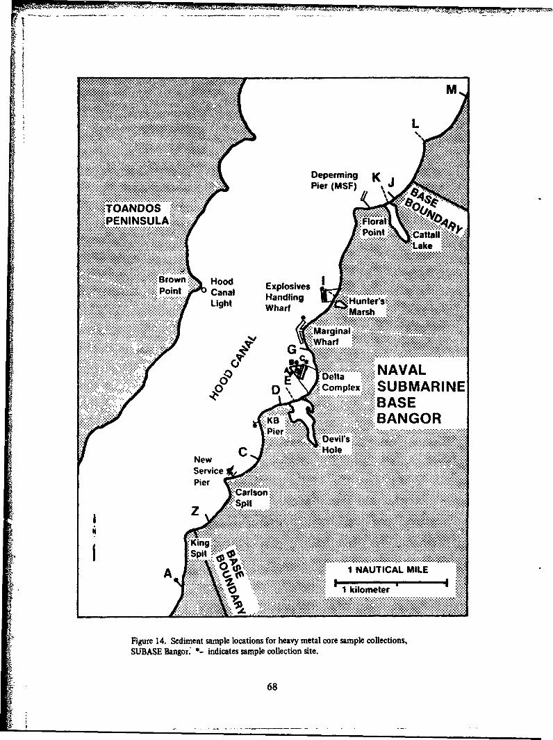
..... M

.~~ . .. . . . . . .. .. . .

....................... ........ x-iI.

.. . . . ... .. . . . ........ Depe.rmin

........PE.N UL .. . .........

*.. ... ... ... ...........................::.? LgtH nlg .uteS::::.............

.. .Ho...........

.. . ............................. %:P o. . .1 NATIA.ML.. ak

SUBASE~.......... 'anor * nictsapljoletinsie

68 . .........

X .4 . . .Ow X.

......4 Deperming.............. .. . .. Pier (M SF)

:::':::-:TOANDOSPENINULA :loral* .. o

Point cati

::C

C..........HoleCRon. coppe rockf.h.(S... te

Ca a c.crab.(Cancr .......tus.. . . .. . . . .

Ha dln o.oyster.C....o..e..g..asLiegccmbrhtrsiccu

. ........ W harfi....

1MaUTCAs ML.. .... ...... .

..... Figure.15..Organismncollection.locations,.heavy.metals... . . . ... . . .. . . . .

................ :'h69

... ..... '. . -. ...". ....

analyses. Forty mussels (Mytilus edulis) ranging from 35-45 mm in length were collectedfrom the -1.0-foot tidal level at each heavy metal sampling station. During the 1980 survey,byssal glands and adductor muscles were dissected out and grouped into pooled samples foreach location. During the 1981 survey, the remaining soft tissues were also retained (in addi-tion to byssal glands and adductor muscles). This design was developed to examine the utili-ty of separate tissue analyses in Mytilus edulis.

With the exception of mussels (consisting of pooled samples), all selected hearymetals specimens were collected and analyzed separately in replicates of three from each site.During laboratory dissections, only glass, plastic and stainless steel instruments and contain-ers were used for specimen handling to avoid contamination. Tissue and sediment sampleswere chilled in the field immediately after collection and frozen within six hours.

Chemical analyses were performed for 1980 and .1981 samples by EnvironmentalEngineering Laboratory in San Diego, California. Sediment and tissue were analyzed accord-ing to Environmental Protection Agency (EPA) procedures. Hot nitric acid reflux was usedduring digestion. Mercury samples were analyzed using a cold vapor technique (EPA Method245.5). Heavy metal analyses were performed using atomic absorption techniques. Tin (Sn)was deleted from the analytical protocol after 1980 samples revealed extremely low levels(below detection limits) in most cases. Heavy metal data are reported in mg/kg dry weight,except for mercury, which is reported in mg/kg wet tissue weight and percent moisture.

RESULTS AND DISCUSSION

The results of heavy metal surveys are presented and discussed in two parts: sedi-.* ments and tissues. The detection limits for specific metals in sediments and tissues are listed

in table 22.

Sediments

The results of sediment heavy metal analyses for samples collected during 1980 and1981 are shown- in table 23. The data are variable, but the presence of military operationsand a characteristic "ship's signature" is evident from samples collected near stations KB andMW, particularly for cooper, lead and zinc. For copper, mercury and lead, values vary greatlybetween 1980 and 1981. Sediments adjacent to northern Marginal Wharf were intensivelysampled during the 1981 survey to validate high mercury levels seen in 1980. The 1981 data,however, show values well within the average ranges for other sampling sites, including thecontrol station, A. Apparently, heavy metal content within the sediments can fluctuatewidely at a single location. Therefore, considerable background data are probably rmquiredto establish a reasonable baseline for valid comparisons.

Tissues

Certain organisms, primarily bivalve molluscs, retain metals in their tissues at con-centrations oftentimes several orders of magnitude greater than levels in surrounding waters.Furthermore, certain organisms may be useful biological monitors for specific heavy metals.The results of heavy metal analyses for selected tissues in several common Hood Canalorganisms are presented and discussed in this section.

70

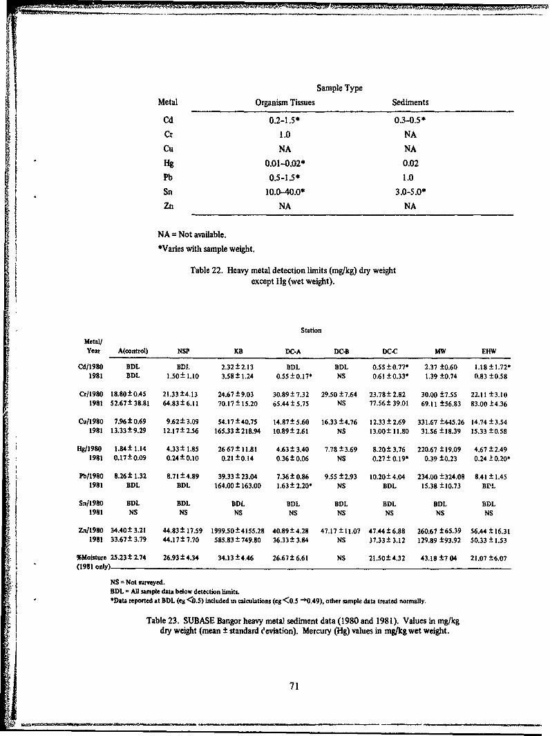
Sample Type

Metal Organism Tissues Sediments

Cd 0.2-1.5* 0.3-0.5*

Cr 1.0 NA

Cu NA NA

Hg 0.01-0.02* 0.02

Pb 0.5-1.5* 1.0

Sn 10.0-40.0* 3.0-5.0*

Zn NA NA

NA = Not available.

*Varies with sample weight.

Table 22. Heavy metal detection limits (mg/kg) dry weightexcept tlg (wet weight).

Station

Metal/Year A(control) NSP KB DC-A DC-B DC-C MW EHW

Cd11980 BDL BDI. 2.32±2.13 BDL BDL 0.55±0.77* 2.37 ±0.60 1.18 ±1.72*1981 BDL 1.50± 1.10 3.58± 1.24 0.55-±0.17* NS 0.61 ±0.330 1.39 ±0.74 0.83 ±0.58

Cr/1980 18.80±-0.45 21.33-±4.13 24.67-±9.03 30.89± 7.32 29.50 ±7.64 23.78± 2.82 30.00 ±7.55 22.11 ±3.101981 52.67± 38.81 64.83 ± 6.11 70.17 ± 15.20 65.44± 5.75 NS 77.56 39.01 69.11 ±56.83 83.00 ±4.36

Cu/1980 7.96-±0.69 9.62±3.09 54.17-±40.75 14.87±5.60 16.33 ±4.76 12.33±2.69 331.67 ±445.26 14.74 ±3.541981 13.33-±9.29 12.17 ± 2.56 165.33-±218.94 10.89± 2.61 NS 13.00± 11.80 31.56 ±18,39 15.33 ±0.58

Hg/1980 1.84± 1.14 4.33±t 1.85 26 67 ± 11.81 4.63± 3.40 7.78 ±3.69 8.20± 3.76 220.67 ±19.09 4.67 ±-2.491981 0.17± 0.09 0.24± 0.10 0.21 ±0.14 0.36± 0.06 NS 0.27± 0.19" 0.39 ±0.23 0.24 ±0.20*

Pb/1980 8.26± 1.32 8.71 ±4.89 39.33 ± 23.04 7.36± 0.86 9.55 ± 2.93 10.20± 4.04 234.00 ±324.08 8.41 ± 1.451981 BDL BDL 164.00 ±163.00 1.63± 2.20* NS BDL 15.38 ±10.73 BE'L

Sn/1980 BDL BDL BDL BDL BDL BDL BDL BDL1981 NS NS NS NS NS NS NS NS

Zn/1980 34.40±3.21 44.83-±17.59 1999.50±4155.28 40.89±4.28 47.17-±11.07 47.44±6.88 260.67 ±65.39 56.44-±16.311981 33.67± 3.79 44.17- ±7.70 585.83± 749.80 36.33± 3.84 NS 37.33-± 3.12 129.89 ±93.92 50.33 ± 1.53

%Moisture 25.23± 2.74 26.93±4.34 34.13 ±-4.46 26.67±-6.61 NS 21.50±-4.32 43.18 ±7 04 21.07 ±6.07(1981 only)

NS = Not surveyed.BDL = All sample data below detection limits.*Data reported at BDL (eg <D.5) included in calculations (eg <0.5 -*0.49), other sample data treated normally.

Table 23. SUBASE Bangor heavy metal sediment data (1980 and 1981). Values in mg/kgdry weight (mean ± standard deviation). Mercury (Hg) values in mg/kg wet weight.

71

Copper Rockfish

Copper rockfish muscle and liver tissue heavy metal data are presented in tables 24and 25. Except for station Z, metal levels were relatively consistent for all stations. At sta-tion Z, copper, lead and zinc values were elevated, especially in liver tissue, relative to otherstations. Rockfish samples were analyzed for heavy metal content at station Z only for sam-ples collected during the 1981 survey. The average length of rockfish specimens at station Zwas 150 mm, whereas the average at other stations approached 200 mm. This size differencemay reflect biotic factors which, in turn, may affect heavy metal levels in tissues. The corn-bined station data indicate that copper rockfish concentrate zinc in liver tissue at concentra-tions above muscle and sediment levels. Copper levels in rockfish liver tissue was similar torespective copper concentrations in sediment samples. The lead content was significantlyelevated in both liver and muscle tissues for rockfish collected in 1981. Unusually low leadlevels measured for 1980 specimens may account for this discrepancy.

Rock Crabs

Rock crab tissue heavy metal data are listed in tables 26 and 27. Heavy metal valuesare relatively consistent between stations. Rock crabs may concentrate cadmium in thehepatopancreas gland. Additionally, hepatopancreas gland cadmium levels are considerablyhigher in 1981 samples than those collected in 1980. Copper, lead and zinc levels are greaterin both crab muscle and hepatopancreas glands than in sediments collected from equivalentlocations. Chromium and mercury levels are low in both tissue types. Again, as with rockfish,lead values were significantly higher for both kinds of crab tissues sampled in 1981 collec-tions than for 1980.

Oysters

Oyster heavy metal tissue data are listed in table 28. Oysters were collected for heavymetal analyses only during the 1981 survey., Station A (control) demonstrates typically lowtissue levels for all heavy metals. Marginal Wharf represents the most heavily impacted sitedue to its operational status during the last two decades. Copper values were similar for oys-ter tissues and sediments collected at Marginal Wharf. These preliminary data indicate thatoysters collected from six SUBASE Bangor intertidal regions accumulate some heavy metalsin their soft tissues. However, the bioconcentration effects do not exceed one order of mag-nitude when compared with equivalent location sediment data.,

Mussels

Mussel tissue heavy metal data are presented in tables 29, 30 and 31. The "general"tissue values shown in table 29 were collected during the 1981 survey and analyzed to eval-

uate the validity of separate tissue dissections for mussels. The "general' tissue consists ofall mussel soft parts minus the adductor muscle and byssal gland tissue which are listed intables 30 and 31, respect*- ely. An analysis of variance performed on these data indicatedthat no significantly different heavy metal information was obtained using separate musseltissues. Therefore, in all subsequent surveys the entire soft parts of pooled (10 individuals)Mytilus edulis samples will be analyzed for each station. Surprisingly, the highest mercurylevels present in mussel tissues were observed at station A, the control station. Copper, lead

72

Station

Metal/Year A(control) Z C D-E1 1

Cd/1980 BDL NS BDL BDL BDLS1981 BDI. BDL BDL BDL BDL

SCr/1980 1.67 ± 0.15 NS 1.05 ± 0.21 1.0 1.13 ± 0.061981 BDL BDL BDL BDL BDL

Cu/1980 3.30± 1.01 NS 2.85 ± 0.92 3.0 2.77 ± 0.321981 3.43 ± 2.80 7.40± 5.72 3.33 ± 2.02 2.50± 0.69 3.00± 1.87

Hg/1980 2 0.17 ± 0.033 NS 0.22 ± 0.08 0.31 0.33 ± 0.051981 0.87 ± 0.28 0.34± 0.04 0.38 ± 0.51 0.17 ± 0.03 0.11± 0.02

Pb/1980 1.80± 0.36 NS 1.35 ± 1.21* BDL 2.07 ± 0.291981 27.67 ± 19.66 35.33 ± 12.70 26.67 ± 18.50 25.33 ± 6.51 22.33 ± 9.71

Sn/1980 BDL NS BDL BDL BDL1981 NS NS NS NS NS

Zn/1980 41.67 ± 4.73 NS 29.00± 8.49 25.0 26.67 ± 2.891981 42.33 ± 20.03 56.67 ± 18.01 31.33 ± 7.09 30.00± 5.00 32.00 ± 5.20

% Moisture 78.93 ± 0.32 78.40± 0.78 79.13 ± 0.76 78.37± 0.15 77.80 ± 0.44(1981 only)

NS = Not surveyed. In = 1 (1980 only).BDL = All sample data below detection limits. 2Tissue type not provided (except :•).*Individual data reported as <x (eg <0.5) 3Muscle tissue data provided only,

included in calculations (eg <0.5 -+0.49), liver tissue data not provided.other sample data treated normally.

Table 24. Rockfish muscle tissue heavy metal data mg/kg dry weightexcept Hg, wet weight, (mean ± standard deviation).

7

73

Station

Metal/Year A(control) Z C D-E1 I

Cd/1980 BDL NS BDL 1.7 1.50 ±0.10

1981 BDL BDL BDL BDL BDL

Cr/1980 16.43 ±-22.14 NS BDL 1.3 BDL

1981 BDL BDL BDL BDL BDL

Cu/1980 15.67 ±1.53 NS 17.00 ± 4.24 12.0 12.67 ±2.52

1981 26.00 ± 15.59 42.00 ± 11.53 21.67 ± 10.50 16.33 ±3.06 25.33 t 2.89

Hg/1980 2 NA 3 NS 0.22 ± 0.08 0.31 0.33 ±0.05

1981 0.11 ± 0.16* 0.95 ±0.02 BDL 0.46 ± 0.04* 0.09 ± 0.14*

Pb/1980 BDL NS BDL BDL BDL

1981 85.00 ± 11.53 130.33 ± 64.08 115.67 ± 64.42 95.67 ± 33.32 74.00 ± 17.78

Sn/1980 BDL NS BDL BDL BDL

1981 NS NS NS NS NS

Zn/1980 225.33 ± 32.08 NS 132.50 ±0.71 170.0 151.67 ±57.711981 159.33 ± 5.03 240.33 ±46.82 178.67 ± 24.01 157.67 ± 19.35 170.33 ± 23.01

% Moisture 65.12 ± 7.41 65.60 ± 1.48 68.23 ± 3.60 67.37 ± 3.36 65.20 ± 2.38(l981lonly) n1l8ol)

NS = Not surveyed. 2 (1980 only).

BDL = All sample data below detection limits. 2Tissue type wot provided (except:3

*Individual data reported as <x (eg <0.5) 3Muscle tissue data provided only,included in calculations (eg <0.5 - 0.49), liver tissue data not provided.other sample data treated normally.

Table 25. Rockfish liver tissue heavy metal data mg/kg dry weightexcept Hg, wet weight, (mean ± standard deviation),

74

Station

Metal/Year A(control) NSP KB D--E G MW EHW

Cd/1980 1.83 ±_2.75* BDL 0.77 ±_0.21 BDL 1.27 ±0.97 0.63 ±0.45 0.80 ±0.411981 BDL BDL BDL BDL BDL 1.17 ±0.25 3.60 ±2.46

cr/1980 0.90± 0.26 0.90± 0.53* 1.37 ± 0.60 0.97 ±0.67* 1.06 ±0.78* 0.56 -+0.06" 1.00 ±0.181981 BDL 1.27± 0.64* 1.67± 1.33* 3.10 ±-3.81" 1.57 ±0.59* BDL BDL

Cu/1980 72.33± 67.40 27.00 ±4.00 14.70±5.80 22.00 ± 5.66 51.00 ± 32.08 10.70 ±2.91 16.25 ±4.721981 23.00± 7.00 17.67± 4.51 24.67± 3.06 26.33± 7.09 21.33± 7.64 23.33± 11.93 36.00± 9.64

Hg/1980 0.24± 0.06 0.19± 0.06 0.33± 0.25 0.25 ± 0.03 0.39 ±0.06 0.19 ±0.02 0.17 ±0.141981 0.15±0.24* 1.05_±0.21 0.22_±0.08 0.46±0.16 0.11-±0.05 0.33±0.15 0.52±0.07

Pb/1980 BDL 0.56± 0.12" BDL 0.61± 0.30* 2.60± 2.17 BDL BDL1981 17.67± 8.96 26.00± 7.81 27.33± 10.07 28.00_±5.00 27.00_±20.66 31.67_±6.66 41.00±4.36

Sn/1980 BDL BDL BDL BDL BDL BDL BDL1981 NS NS NS NS NS NS NS

Zn/1980 406.33± 55.90 339.00± 35.04 405.00± 28.69 322.17 ± 35.86 391.00 ± 42.33 378.00 ± 15.72 321.50± 62.681981 342.67± 48.18 341.00± 65.64 405.67± 17.93 413.67± 11.37 348.00± 26.15 370.67-±89.02 334.33± 20.98

% Moisture 75.83± 2.23 76.63± 0.64 77.90± 0.00 78.60± 4.93 81.57 ± 6.34 77.97 ± 0.67 77.60 ± 1.65(1981 only)

NS = Not surveyed.

BDL = All sample data below detection limits.

*Individual data reported as <x (eg <0.5) included in calculatiwu (eg <0.5 -- 0.49); other sample data treated normally,

Table 26. Crab muscle tissue heavy metal data in mg/kg dry weight except Hg,wet weight, (mean ± standard deviation).

75

Station

Metal/Year A(control) NSP KB D-E G MW EHW

Cd/1980 13.33 ±1.53 19.33 ±7.77 10.53 ±1.75 21.00 ±S.29 12.67 ±1,53 13.37 ±6.07 13.25 ±2.631981 43.33 ± 18.90 74.67 ±21.94 99.67 ±8.08 44.00 ±19.31 68.33 ±8.50 42.00 ±12.49 50.00 ±4.36

Cr/1980 BDL 1.46± 0.55* BDL 3.20 ± 2.51 BDL BDL BDL1981 BDL 1.23± 0.31" 3.07± 1.59 4.10± 1.71 2.30± 1.31" 2.73± 1.25 2.30± 2.34

Cu/1980 34.33± 13.65 52.33±9.29 18.33 ±5.13 53.00 ±27.22 35.67 ±8.02 41.33 ±19.86 19.75 ±2.361981 29.33± 5.13 34.00± 16.70 39.67 ± 21.39 32.00 ±27.73 18.33 ±6.35 23.00 ±5.29 34.33 ±7.37

Hg/1980 0.27± 0.16 0.12± 0.03 0.07± 0.02 0.13± 0.10* 0.11 ± 0.07 0.35± 0.07 0.16± 0.29*1981 0.07± 0.10* 0.37± 0.07 0.10± 0.09* 0.14 ± 0.09 BDL 0.08 ±0.04 0.26 ±0.12

Pb/1980 BDL BDL BDL 2.86± 1.24* 1.10±0.35* BDL BDL1981 18.67± 2.31 27.00± 13.23 26.33± 8.50 25.17± 23.55 68.33 ± 37.53 29.00± 19.29 37.33± 4.16

Sn/1980 BDL BDL BDL BDL IDL BDL BDL1981 NS NS NS NS NS NS NS

Zn/1980 193.33± 15.37 175.67± 2.31 209.33± 47.65 206.67± 30.24 201.33±46.00 248.00± 91.76 225.25± 31.821981 157.33± 51.29 301.00± 120.38 281.67± 106.40 269.00± 100.95 492.67± 317.31 271.67± 27.54 226.00± 33.72

% Moisture 71.70± 1.67 73.53± 4.63 72.57± 5.15 75.30± 6.94 76.87 ± 8.11 76.07± 5.58 77.73± 3.62(1981 only)

NS = Not surveyed.

BDL = All sample data below detection limits.*Individual data reported as <x (eg e0.5) included in calculations (eg <0.5 -10.49); other sample data treated normally.

Table 27. Crab hepatopancreas tissue heavy metal data mg/kg dry weight except Hg,wet weight, (mean ± standard deviation).

Station

Metal A(control) NSP DC D-E MW EHW

Cd 9.43 ± 3.50 12.23 ± 4.29 12.67 ± 2.31 19.00 ± 4.00 18.67 ± 0.58 15.53 ± 7.71

Cr 0.76 ± 1.16* 1.73 ± 0.80* BDL BDL BDL BDLCu 27.67 ± 4.93 81.33 ± 19.35 81.00 ± 28.16 106.33 ± 35.50 256.00 ± 88.71 181.00 ± 109.05Hg 0.10 ± 0.07 BDL BDL 0.14 ± 0.11" 0.03 1- 0.03* BDLPb 9.43 ± 5.13 20.67 ± 4.73 23.00 ± 12.53 11.30 ± 5.74 39.67 :l: 15.04 14.00 ± 4.00

Sn NS NS NS NS NS NSZn 572.33 ± 198.53 1520.67 ± 720.60 956.67 ± 337.51 1413.67 ± 340.08 2363.33 ± 715.95 2247.67 ± 1058.77

% Moisture 73.80 ± 3.26 73.93 ± 1.02 80.40 ± 2.10 75.57 ± 0.76 82.00 ± 1.48 79.23 ± 3.02

NS = Not surveyed.BDL All sample data below detection limits.*Individual data reported as <x (eg <•0.5) included in calculations (eg <0.5 "40.49); other

sample data treated normally.

Table 28. Oyster tissue heavy metal data (1981 only) mg/kg dry weight except Hg,wet weight, (mean ± standard deviation).

76

Station

Metal A(control) NSP KB DC MW EHW

Cd 9.8 3.8 5.5 12.0 4.9 11.0

Cr < 1.0 2.5 < 1.0 <1,0 < 1.0 1.1

Cu 11.0 11.0 18.0 8.6 11.0 14.0-

Hg 0.53 0.18 0.07 0.54 0.51 0.26

Pb 49.0 28.0 31.0 60.0 39.0 35.0

Sn NS NS NS NS NS NS

Zn 153.0 120.0 159.0 196.0 146.0 158.0

% Moisture 80.3 80.7 82.3 83.3 82.7 83.3

NS = Not Surveyed.

Table 29. Mytilus general tissue heavy metal data (1981 only) mg/kg dry weight except Hg, wet weight.

Station

Metal/Year A(control) NSP KB DC MW EHW

Cd/1980 3.3 4.1 3.7 2.5 3.3 2.21981 < 1.0 < 1.0 < 1.0 3.0 1.9 5.4

, Cr/1980 <2.0 < 1.5 < 1.5 < 1.5 < 1.5 < 1.51981 3.5 < 1.0 < 1.0 < 1.0 < 1.0 < 1.0

Cu/1980 22.0 18.0 17.0 14.0 14.0 9.61981 6.9 7.7 16.0 3.0 7.7 5.4

Hg/1980 1.37 0.05 0.38 0.09 <0.02 0.171981 0.60 0.13 0.31 0.77 0.24 0.21

Pb/1980 10.0 4.1 < 1.5 < 1.5 < 1.5 < 1.01981 41.0 73.0 123.0 40.0 46.0 54.0

SSn/1980 <40 0 <40.0 <40.0 <40.0 <40.0 <30.01981 NS NS NS NS NS NS

Zn/1980 199.0 243.0 207.0 283.0 158.0 103.01981 149.0 172.0 207.0 165.0 132.0 149.0

% Moisture 78.1 78.0 76.7 78.5 78.4 77.5(1981 only)

NS = Not surveyed.

Table 30. Mytflus muscle tissue heavy metal data (1980-1981) mg/kg dry weight except Hg, wet weight.,

77

Staton

Metal/Year A(control) NSP KB DC MW EHW

Cd/1980 6.7 5.5 7.0 5.5 6.4 4.71981 5.4 6.0 2.6 3.6 1.1 4.3

Cr/1980 7.4 11.0 7.4 <0.6 3.5 3.61981 6.9 3.6 < 1.0 < 1.0 < 1.0 < 1.0

Cu/1980 25.0 23.0 20.0 15.0 28.0 14.01981 6.9 9.6 10.0 7.1 6.7 7.5

Hg/1980 1.15 0.41 0.39 0.44 0.66 0.221981 0.71 0.08 0.24 0.62 0.43 0.39

Pb/1980 7.4 4.6 18.0 7.1 2.9 5.21981 25.0 24.0 37.0 29.0 27.0 25.0

Sn/1980 < 30.0 < 20.0 < 20.0 <20.0 <20.0 < 10.01981 NS NS NS NS NS NS

Zn/1980 185.00 180.0 228.0 200.0 172.0 217.01981 141.0 120.0 116.0 102.0 106.0 90.0

% Moisture 76.8 77.7 76.9 78.4 79.4 79.8(1981 only)

NS = Not surveyed.,

Table 31., Mytilus byssal gland tissue heavy metal data (1980-198 1) mg/kg dry weight except Hg, wet weight.

78

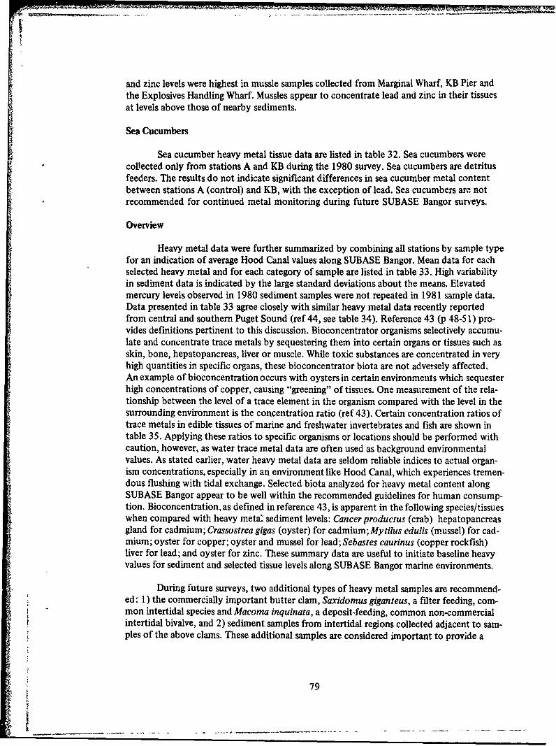
and zinc levels were highest in mussle samples collected from Marginal Wharf, KB Pier andthe Explosives Handling Wharf. Mussles appear to concentrate lead and zinc in their tissuesat levels above those of nearby sediments.

Sea Cucumbers

Sea cucumber heavy metal tissue data are listed in table 32. Sea cucumbers werecollected only from stations A and KB during the 1980 survey. Sea cucumbers are detritusfeeders. The results do not indicate significant differences in sea cucumber metal contentbetween stations A (control) and KB, with the exception of lead. Sea cucumbers are notrecommended for continued metal monitoring during future SUBASE Bangor surveys.

Overview

Heavy metal data were further summarized by combining all stations by sample typefor an indication of average Hood Canal values along SUBASE Bangor. Mean data for eachselected heavy metal and for each category of sample are listed in table 33. High variabilityin sediment data is indicated by the large standard deviations about the means. Elevatedmercury levels observed in 1980 sediment samples were not repeated in 1981 sample data.Data presented in table 33 agree closely with similar heavy metal data recently reportedfrom centrai and southern Puget Sound (ref 44, see table 34). Reference 43 (p 48-51) pro-vides definitions pertinent to this discussion. Bioconcentrator organisms selectively accumu-late and concentrate trace metals by sequestering them into certain organs or tissues such asskin, bone, hepatopancreas, liver or muscle. While toxic substances are concentrated in veryhigh quantities in specific organs, these bioconcentrator biota are not adversely affected..An example of bioconcentration occurs with oysters in certain environments which sequesterhigh concentrations of copper, causing "greening" of tissues. One measurement of the rela-tionship between the level of a trace element in the organism compared with the level in thesurrounding environment is the concentration ratio (ref 43). Certain concentration ratios oftrace metals in edible tissues of marine and freshwater invertebrates and fish are shown intable 35. Applying these ratios to specific organisms or locations should be performed withcaution, however, as water trace metal data are often used as background environmentalvalues. As stated earlier, water heavy metal data are seldom reliable indices to actual organ-ism concentrations, especially in an environment like Hood Canal, which experiences tremen-dous flushing with tidal exchange. Selected biota analyzed for heavy metal content alongSUBASE Bangor appear to be well within the recommended guidelines for human consump-tion. Bioconcentration, as defined in reference 43, is apparent in the following species/tissueswhen compared with heavy meta: sediment levels: Cancer productus (crab) hepatopancreasgland for cadmium; Crassostrea gigas (oyster) for cadmium; Mytilus edulis (mussel) for cad-mium; oyster for copper; oyster and mussel for lead; Sebastes caurinus (copper rockfish)liver for lead; and oyster for zinc. These summary data are useful to initiate baseline heavyvalues for sediment and selected tissue levels along SUBASE Bangor marine environments.

During future surveys, two additional types of heavy metal samples are recommend-ed:- 1) the commercially important butter clam, Saxidomus giganteus, a filter feeding, com-mon intertidal species and Macoma inquinata, a deposit-feeding, common non-commercialintertidal bivalve, and 2) sediment samples from intertidal regions collected adjacent to sam-ples of the above clams. These additional samples are considered important to provide a

79

Station

Metal/Year A(control) KB

Cd/1980 BDL 1.75 ± 0.07

Cr/1980 1.43 ±0.22 1.75 ± 0.92Cu/1980 3.73 ± 1.02 9.35 ± 2.33Hg/1980 0.03 ±0.03* 0.31 ± 0.30Pb/1980 1.02 ±0.42* 5.30 ± 0.42Sn/1980 BDL BDLZn/1980 118.50 ±4.36 147.50 ± 17.68

BDL = All sample data below detaction limits.

*Individual data reported as <x (eg <0.05) included incalculations (eg <0.5 -+0.49); other sample data treatednormally.

Table 32. Paralschopus californicus (sea cucumber) muscle tissue heavy metal data (1980 only).Values in m&gkg dry weight except Hg, wet weight (mean ± standard deviation).

80

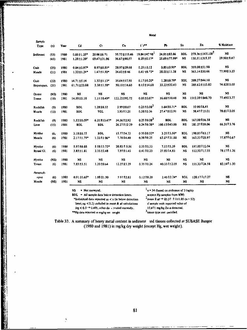
Metal

SampleType (n) Year Cd Cr Cu It" P** Sn Zn %Moisture

Sediment (53) 1980 0.85±1.250 25.06±6.71 35.72±115.46 19.84W49 Q81 24.95±82.86 BDL 279.36±1431.082 NS

(45) 1981 1.28±1.20e 69.47±31.96 36.67±90.57 0.29±0.170 25.69±77.99* NS 130.31±315.37 29.50±9.47

Crab (25) 1980 0.84±0.970 0.97±0.500 28.97±29.68 0.251 0.12 0.85 ±0.95* BDL 359.08±51.98 NS

Muscle (21) 1981 1.32±1.24* 1.47±1.50" 24.62±846 0.41t"0.'3* 28.00±11.28 NS 365.14±50.66 77.99±3.23

Crab (22) 1980 14.71±5.14 1.32±1.13" 35.64±17.95 0.17±0.20" 1.28±0.79" BDL 209.27±44.10 NS

Hepatopan. (21) 1981 61.71±23.08 2.38±1.58" 30.10±14.60 0.15±14.60 33.23±22.43 NS 285.62±153.82 74.82±5.05

Oyster (NS) 1980 NS NS NS NS NS NS NS NS

Tissue (18) 1981 14.59±5.10 1.11±0.490 122.22±92.72 0.05±0.07' 16.68±10.48 NS 1512.39±848.70 77.49±3.77

Rockfish (9) 1980 BDL 1.28±0.32 299±0.67 0.25±0.083 1.64±0.71' BDL 3200±8.41 NS

Muscle (15) 1981 BDL 9DL 3.93-±3.21 0.38±0.36 27.47±12.91 NS 38.47±15.01 78.01±2.05

Rockfish (9) 1980 1.52±0.09* 6.21±13.47" 14.56±2.92 0.25 ±0.083 BDL BDL 167.00±56.58 NS

Liver (15) 1981 BDL BDL 26.27±12 29 0.24±0.38* 100.13±43.00 NS 181.27±39.06 66.31±3.76

Mytiaus (6, 1980 3.18±0.72 BDL 15.17±4.23 0 35_±0.52* 3.25±3.50* BDL 198.83±63.17 NSMuscle (6) 1981 2.17±1.79' 1.33±1 06* 7.78±4.40 0.38±0.25 62.81±31.88 NS 162.33±25.97 77.87±0.67

Mytius (6) 1980 5.97±0.88 5 58±3.72* 20.83 ±5.56 0.55 ±0.33 7.53±5.39 BDL 197.00±22.04 NS

Byssal GI. (6) 1981 3.83±1.81 2.35 ±2.48 7.97±1.45 0.41 ±0.23 27.83±-4.83 NS 112.50±17.55 78.17±+1.26

Mytlus (NS) 1980 NS NS NS NS NS NS NS NSTiqsue (6) 1981 7.83_±3.51 1.20±0.64 12.27 ±3.29 0.35_±0.24 40.33±12.09 NS 155.33±24.58 82.10±1.30

Parastich."opus (6) 1980 0.91 ±0.65* 1.88±+.30 5 97±2.82 0.12±0.20 2.45±2.24* BDL 128.17±17.27 NS

Muscle (NS) 1981 NS NS NS NS NS NS NS NS

NS = Not surveyed. In = 54 (based on inclusion of 3 highly

BDL = All sample data below detection limits. suspect Hg samples from MW)

"Individual data reported as < x (ie below detection -mean ± sd -- 83.37 ± 111.05 (n = 52)

limit; eg <0.5) included in mean & sd calculations if sample with reported value of

(eg < 0.5 - 0.49), other da i sr-ated normally. 10,471 mg/kg Zn is detected.

"•*Hg data reported in mg/kg we weight 3 tissue type not ,pecified.

Table 33. A summary of heavy metal content in sediment md tissues collected at SUBASE Bangor(1980 and 1981) in mg/kg dry weight (except Hg, wet weight).

81

Mean Minimum Maximum Coefficient

Concentration Concentration Concentration of(ppm) (ppm) (ppm) variation (%)

Metal:

Arsenic 27.56 0.00 472.00 319

Lead 103.84 7.93 793.00 148

Copper 116.59 10.20 1602.00 210

Zinc 153.99 23.20 1720.00 170

Mercury 0.40 0.02 1.38 95

Selenium 29.47 9.30 113.00 72

Cadmium 7.27 3.08 18.30 43

Chromium 41.87 20.90 71.50 33

Table 34. Sediment heavy metal data listed in reference 44, for comparison with SUBASE Bangor data.

Statistics are for 41 Puget Sound sampling stations (MESA Project).

Marinu Freshwater

Invertebrates Fish Invertebrates Fish

Antimony 0.005 0.04 0.01 0.001

Arsenic 0.333 0.333 0.333 0.333

Beryllium 0.2 0.2 0.01 0.002

Cadmium 50.0 3.0 2.0 0.2

Chromium 2.0 0.4 0.04 0.04

CobaX 1.0 0.1 0.2 0.02

Copper 1.67 0.667 1.0 0.2

Lead 1.0 0.3 0.1 0.3

Mercury 33.3 1.67 100.0 1.0

Nickel 0.25 0.1 0.1 0.1

Selenium 1.0 4.0 0.167 0.167

Tin 1.0 3.0 1.0 3.0

Vanaaium 0.05 0.01 3.0 0.01

Source: Adapted from reference 52.

Table 35. Data listed for comparison with SUBASE BANGOR data.' conc, ntration ratios of trace metalsin edible tissues of invertebrates and fish (X 1,000 ppm) (ref 43)

82

more comprehensive evaluation of intertidal metal burdens along SUBASE Bangor. Futuresurveys will include these data and serve to monitor key elements in the Hood Canalecosystem.

CONCLUSIONS

1. Heavy metal data collected during 1980 and 1981 indicate that levels present

along SUBASE Bangor are similar to other areas of Puget Sound.

S2. Sediment data are highly variable with respect to heavy metal content at a givenS, location.

3. Selected tissue monitoring for heavy metal content is a potentially useful aspectof SUBASE Bangor environmental monitoring surveys.

4. Resident Hood Canal species such as oysters, mussels, crabs and rockfish havebeen seen to bioconcentrate certain heavy metals.

5. The establishment of a heavy metal baseline is important for continued moni-toring of key elements of the marine ecosystem at SUBASE Bangor.

83

REF..RENCES

1., Naval Undersea Center TP 510, Trident Biological Surveys: A summary report, June1973-July 1975, by TJ Peeling and HW Goforth, 14 4 p, 1975.

2. Naval Undersea Center TP 5110 (Supplement 1), Trident Biological Survey: July 1976,by TJ Peeling, MH Salazar, JG Grovhoug and HW Goforth, 58p, 1976.

3. Naval Ocean Systems Center TR 513 (Supplement 2 to NUC TP 510), Trident Biolog-ical Surveys: SUBASE Bangor (July 1977 and June 1978) and Indian Island Annex(January, May 1074 and June 1978), HW Goforth, TJ Peeling, MH Salazar and JGGrovhoug, 84p, 1979.

4. Simenstad, CA, Prey Organisms and Prey Community Composition of Juvenile Salmon-ids in Hood Canal, Washington, paper presented at 1st Pacific Northwest Workshop onFish Food Habit Studies, Astoria, Oregon, 13-15 October 1976, p 163-176, 1976.

5., Simenstad, CA, Miller. BS, Nyblade, CF, Thornburgh, K, and Bledsoe, CF, Relation-ships of Northern Puget Sound and the Strait of Juan de Fuca: a synthesis of availableknowledge, MESA Puget Sound Project/EPA-600/7-79-259, 33 5p, 1979.

6. Salo, EO, Bax, NJ, Prinslow, TE, Whitmus, CJ, Snyder, BP, and Simenstad, CA, TheEffects of Construction of Naval Facilities on the Outmigration of Juvenile Salmonidsfrom Hood Canal, Washington, Fisheries Research Institute, University of Washington,FRI-UW-8006, 150p, 1980.

7. Allen,GH, DeLacy, AC, and Gotshall, DW Quantitative Sampling of Marine Fishes - aproblem in fish behavior and fishing gear, in Waste Disposal in the Marine Environment,p 448-511, 1960.

8. Eggers, DM, Factors in Interpreting Data Obtained by Diel Sampling of Fish Stomachs,Journal Fisheries Research Board of Canada, vol 34, p 290-294, 1977.

9. Greening, HS, and Livingston, RL Diel Variation in the Structure of Seagrass-associatedEpibenthic Macroinvertebrate Communities, Marine Ecology, vol 7, p 147-156, 1982.

10. Hart, JL, Pacific Fishes of Canada, Fisheres Research Board of Canada Bulleiin 180,740p, 1973.,

11. Miller, DJ, and Lea, RN, Guide lo the Coabtal ,,arrpe Fishes of California, CaliforniaDept of Fish and Game Fish Bulletin 157, 235p, 19 .2.

12. Clemens, WA, and Wilby, GV, Fishes of the Pacific ('oa. )f Canada, 2d ed, FisheriesResearch Board of Canada Bulletin 68, 443p, 1961.,

13. DeLacy, AC, Miller, BS, and Borton, SF, Checklist of Piget Sound Fishes, College ofFisheries, University of Washington Contr. 371, 1972.

84

14. Wingert, RC, McCain, BB, Pierce, KV, Borton, SF, Griggs, DT, and Miller, BS, Ecologi-cal and Disease Studies of Demersal Fishes in the Vicinity of Sewage Outfalls, Collegeof Fisheries, University of Washington Contr 444, p 29-30, 1976.

15. Patten, BJ, Biological Information on Copper Rockfish in Puget Sound, Washington,

Trans Am Fisheries Society, vol 102, p 412-416, 1973.

16. Prince, ED, Food of the Copper Rockfish, Sebastes caurinus Richardson, Associatedwith an Artificial Reef in South Humboldt Bay, California, California Fish and Game,vol 62, p 274-285, 1976.

17. Forrester, CR, and Thompson, JA Population Studies on the Rock Sole (Lepidopsettabilineata) of Northern Hecate Strait, British Columbia, Fisheries Research Board ofCanada Tech Report 108, 104p, 19 9.

18. Orcutt, HG, The Life History of the Starry Flounder, California Dept of Fish andGame Fish Bulletin 78, 64p, 1950.

19. Jones, BC, and Geen, GH, Food and Feeding Habits of Spiny Dogfish (Squalus acan-thias) in British Columbia Waters, Journal Fisheries Research Board of Canada, vol 34,p 2067-2078, 1977.

20. Amos, MH, Commercial Clams of the North American Pacific Coast, Bureau of Com-mercial Fisheries Circular 237, 18p, 1966,

21. Chew, KK, Prospects for Successful Manila Clam Seeding, College of Fisheries, Univer-sity of Washington Contr 440, 13p, 1975.

22. Magoon, C, and Vining, R, Introduction to Shellfish Aquaculture in the Puget SoundRegion, Division of Marine Land Management, Washington Dept of Natural Resources,68p, 1981.

23. Quayle, DB, Distribution of Introduced Marine Mollusca in British Columbia Waters,Journal Fisheries Research Board of Canada, vol 21, p 1155-1181, 1964.

24. Westley, RE. The Oyster Producing Potential of Puget Sound, Proc. National Shell-fisheries Assoc, vol 61, p 20-23, 1971.

25. Smith, RI, and Carlton, JT, Light's Manual: Intertidal Invertebrates of the CentralC.Aifornia Coast, 3d ed, p 562, University of California Press, 1975.

26. Emery, KO, A Simple Method of Measuring Beach Profiles, Limnology and Oceano-graphy, vol 6, p 90-93, 1966.

27. Cornwall, IE, Barnales of British Columbia, British Columbia Provincial MuseumHandbook 7, 69p, 1970.

28. Griffith, LM, The Intertidal Univalves, British Columbia Provincial Museum Handbook26, 101p, 1975,

85

29. Kozloff, EN, Seashore Life of Puget Sound, the Strait of Georgia, and the San JuanArchipelago, University of Washington Press, 281 p, 1973.

30. Kozloff, EN, Keys to the Marine Invertebrates of Puget Sound, the San Juan Archi-pelago, and Adjacent Regions, University of Washington Pless, 226p, 1974.

31. Quayle, DB, The Intertidal Bivalves of British Columbia, British Columbia ProvincialMuseum Handbook 17, 104 p, 1973.

32. Dunnill, RM, and Ellis, DV, Recent species of the genus Macoma (Pelecypoda) in BritishColumbia, National Museum of Ottawa, Canada, Natural History Papers, vol 45, p 1-35,1969.

33. Ricketts, EF and Calvin, J, Between Pacific Tides, 4th ed, 614p, Stanford UniversityPress, 1958.

34. Alexander, GV and Young, DR, Trace Metals in Southern Californian Mussels, MarinePollution Bulletin, vol 7, p 7-9, 1976.

35. Ayling, GM, Uptake of Cadmium, Zinc, Copper, Lead and Chromium hi the PacificOyster, Crassostrea gigas, Grown in Tamar River, Tasmania, Water Research, vol 8,p 729-738, 1974.

36., Bloom, H, and Ayling, GM, Heavy Metals in Derwent Estuary, Environmental Geology,vol 2, p 3-22, 1977..

37. Dairacott, A, and Watling, W, The Use of Molluscs to Monitor Cadmium levels in Es-tuaries and Coastal Marine Environments, Trans Royal Society of South Africa, vol 41,p325-338, 1975..

38. Emerson, RR, Soule, DF, and Oguri, M, Heavy Metal Concentrations in Marine Organ-isms and Sediments Collected Near an Industrial Waste Outfall, Allan Hancock Foun-dation USC Seagrant Publ R-02-76, p 1-5 1976.

39. Frazier, JM, The Dynamics of Metals in the American Oyster, Crassostrea virginica.1. Seasonal Effects, Chesapeake Science, vol 16, p 162-171, 1976.

40. Fra.-'er, JM, The Dynamics of Metals in the American Oyster, Crassostrea virginica.2. Environmental Effects, Chesapeake Science, vol 17, p ±88-197, 1976.

41.. Goldberg, ED, et al, The Mussel Watch, Environmental Conservation, vol 5, p 101-125,1978..

42. Hugget, RJ, Bender, ME, and Sloane, HD, Utilizing Metal Concentration Relationshipsin the Eastern Oyster (Crassostrea virginica) to Detect Heavy Metal Pollution, WaterResearch, vol 7, p 451-460, 1973.

86

43. Jenkins, DW, Biological Monitoring of Toxic Trace Metals: Biological Monitoring andSurveillance, EPA-600[3-80-089, 215p, 1980.

44. Malins, DC, McCain, BB, Brown, DW, Sparks, AK, and Hodgins, HG, Chemical Conta-minants and Biological Abnormalities in Central and Southern Puget Sound, NOAATech Memorandum OMPA-2, MESA Puget Sound Project, 295p, 1980.

45. Miyahara, S, Pollution of Sea Depending on the Heavy Metals and Oils: Annual Varia-tion of Mercury and Cadmium in Seawater and Fundamental Properties of Floating Oil,Nagasaki University, Faculty of Fisheries Report, 15p, 1976.

46. Phillips, DJH Yim, WW-S, A Comparative Evaluation of Oysters, Mussels and Sedimentsas Indicators of Trace Metals in Hong Kong Waters, Marine Ecology, vol 6, p 285-293,1981.

47.. Thompson, JAJ, Paton, DW, Heavy Metals in Benthic Organisms from Point GreyDumpsite, Vancouver, BC:' a preliminary report, Pacific Marine Science Rept, 18p,1978.,

48. Topping, G, Heavy Metals in Fish from Scottish Waters, Aquaculture, vol 1, p 373-377,1973.

A 49, Trefry, JH, and Presley, BJ, Heavy Metals in Sediments from San Antonio Bay and theNorthwest Gulf of Mexico, Environmental Geology, vol 1, 283-294, 1976.

50. Windom, H, Stickney, R, Smith, R, White, D, and Taylor, F, Arsenic, Cadmium,Copper, Mercury, and Zinc in Some Species of North Atlantic Finfish, Journal Fisher-ies Research Board of Canada, vol 30, p 275-279, 1973..

51. Naval Undersea Center TP 457, Heavy Metal Contamination from Navy Ship Hulls, byS Yamamoto, JB Alcauskas, WH Shipman, RH Wade and RR Kenis, 34p, 1975.

52.. Vaughan, BE, Abel, KH, Cataldc "A, Hales, JM, Hane, CE, Rancitelli, LA, Roufson,RC, Wildung, RE, and Wolf, EG, ..-¢/iew of Potential Impact on Health and Environ-mental Quality from Metals Entering the Environment as a Result of Coal Utilization,Battelle Energy Project, North-West Laboratory, 3 50p, 1975.

87

A-... .• "

APPENJIX A

SUBASE BANGOR SAMPLING STATIONS

MNMW4PAMB SLAK- n

89

Station Latitude (N) Longitude (W) Bearing (Magnetic)

0 t it 0 1 "i 0

A 47-42-51.5 122-44-50.0 25047-42-51.0 122-44-53.0

Z 47-43-28.0 122-44-36.0 3054743-29.0 12244-37.0

*Active C 4743-53.0 122-44-20.0 270

Stations 47-43-53.5 122-44-21.0

D 4744-14.5 12244-04.0 32247-44-19.0 122-44-06.5

G 47-44-41.5 122-43-35.5 3104744-42.5 122-43-36.0

J 4746-16.0 12242-17.5 2904746-20.0 12242-26.0

M 4746-58.0 12241-14.0 2604746-58.5 12241-19.0

L 47-46-30.0 122-42-03.0 31047-46-33.0 12242-04.5

K 47-46-11.0 122-42-25.5 32047-46-18.0 122-42-28.0

"Inactive FA 47-4545.0 12243-03.0 300

Stations 47-45-45.5 12243-06.0

E 47-44-15.0 12243-55.5 3154744-22.0 122-44-01.0

CS 4743-47.0 122-44-36.0 340474349.0 12244-36.0

I 4745.16.5 12243-14.0 28047-45-17.5 122-43-19.0

*As of June 1981.,

"**Station M was deleted after 1979; stations L, K & E were deleted after 1978; station FA & CS were

deleted after 1977; station I was deleted after 1974.

Note: Intertidal sampling data were collected at the following stations during the years indicated:-1973-1981." A, C & G;, 1973-1974. I; 1973-1978." E, K & L; 1975-1981: Z; 1977 only:CS & FA; 1979 only: M; 1979-1981: D & J.,

Table A-1. SUBASE Bangor sampling stations: intertidal transects (first Lat/Long indicated position at extremehigh tide mark for 12.0 feet; second Lat/Long indicates position at extreme low tide mark for -3.5 feet).

90

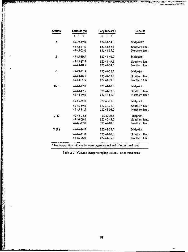
Station Latitude (N) Longitude (W) RemarksS0 1 ff 0 t I

A 47--42-49.0 122-44-54.0 Midpoint*

47-42-275 122.44-52.5 Southern limit4743-03.0 12244-55.0 Northern limit

z 4743-30.5 12244-40.0 Midpoint

47-43-17.5 12244-49.5 Southern limit47-43-40.5 12244-34.5 Northern limit

C 4743-55.5 12244-22.5 Midpoint

47-43-49.5 122-44-32.0 Southern limit4743-05.5 12244-19.0 Northern limit

D-E 4744-27.0 122-44-07.5 Midpoint

47-44-12.5 12244-22.5 Southern limit4744-29.0 12243-51.0 Northern limit

4745-35.0 12243-11.0 Midpoint

4745-19.0 12243.-21.0 Southern limit4745-51.5 12243-04.0 Northern limit

J-K 4746-22.5 12242-24.5 Midpoint4746-09.0 1224243.5 Southern limit4746-32.0 12242-09.0 Northern limit

M (L) 47-46-44.0 122-41-38.5 Midpoint

4746-35.0 12241-07.0 Southern limit4746-58.0 12241-35.5 Northern limit

*denotes position midway between beginning and end of otter trawl haul.

Table A-2., SUBASE Bangor sampling stations: otter trawl hauls.,

91

Station Latitude (N) Longitude (W) Depth0 , ,, (meters)

A 47-42-49.0 122-44-54.0 10

NSP (A) 4743-50.5 122-44-29.5 10(B) 4743-51.5 122-44-30.0 12

KB (A) 47-44-06.0 122-44-18.5 8(B) 47-44"06.5 12244-19.5 12

DC (Al) 47-44-30.5 122-44-00.0 15(A2) 4744-31.0 12z-4 3-57.0 15(A3) 47-44-31.5 122-43-52.5 15(BI) 4744-35.5 122-43-47.0 16(B2) 4744-37.5 122-43-46.0 18(B3) 47.44-39.0 1224344.0 15

MW (Al) 4745.54.5 12243.34.0 12(A2) 4745.55.5 12243-33.0 12(A3) 4745-57.5 12243-30.0 12

EHW 4745-18.5 1224?.23.0 30

Table A-3. SUBASE Bangor sampling stations: sediments, heavy metals.

'9

92

Station Latitude (N) Longitude (W)0 Ft t 0 ift

A 47-42-51.0 122-44-50.0

NSP 47-43-49.0 122-44-285

D-E 4744-22.0 122-43-52.0

DC 47-44-34.5 1224344.0

MW(S) 4744-43.5 12243-34.5

MW(N) 4744-55.5 122-43-28.5

EHW 4745-18.0 122-43-17.0

Table A-4. SUBASE Bangor sampling stations: oysters, heavy metals.

Station Latitude (N) Longitude (W)

0 t 0 1 F?

A 47-42-49.0 122-44-53.0

NSP 47-43-50.0 122-44-29.5

KB 4744"05.5 12244-18.0

DC 47-44-34.5 122-43-44.0

MW(N) 47-44-55.5 122-43-28.5

EHW 47-45-18.5 122-43-19.5

Table A5. SUBASE Bangor sampling stations: mussels, heamy metals.

Station Latituc,. (N) Longitude (W)

0 1 1F 0 1 It

A 4742-51.5 12244-53.0

NSP 4743-50.0 12244-29.0

KB 4744-0.0 12244-19.0

D 47-44-19.0 122-44-06.5

G 474442.5 122-43-36.0

EHW 4745-18.5 12243-19.5

Table A-6. SUBASE Bangor sampling stations: red rock crabs, heavy metals.

93

APPENDIX B

FISH TRAWL CATCH DATA

I9M5D& PAW 26094M 1"M

95

Station

Species A C D-E I J-K M Z Total

Squalus acanthias 1 1

Hydrolagus colieie 1 ____ ____ ___ 1 2

Porichthys notatus ____________ ________ ________

Gadu s macrocephalus________

Merluccius productus 8 8Microgadus proximus 12 3Aulorhynchusflavidus 2 + + 3 5

Gasterosteus aculeatus 2 2

Syngnathus leptorhynchus 3 1 1 2 7Cymatogaster aggregata 14 7 5 9 19 12 3 69

Ernbiotoca lateralis 21 4 1 3 3 7 1 40

Rharochilus vacca I___ I___

Anoplarchus purpurescens ____________ ________ __

Lumpeneus sagitta I___ I___

Apodichthysflavidtis 1 1 2 1 5

Phofi, laeta 1 1 2

Pholis ornata 7 1 8Ammodytes hexapterus ____ ____ _______ _____ ____

Coryphopterus nicholsi ____________ ________ ________

Sebastes caurinus 88 13 5 -9 12 127

Hexagrammos stellepi 1 1

Artedius fenestralisArtedius lat era) is

Clinocottus acuticeps ____

Enophrys bison________

Hemifepidotus hemilepidotus ___ ___ ___ ___ ___

Leptocottus arnnatus 13 1 3 3 1 1 22

Nautichthys oculofasciatus____

Psychrolutes paradoxus11Scorpaenichthys marmoratus 1I

Agonus acipenserinusCitharichthys sordidus ________ ___ ________

Lepidopsetta bilineata ____ ________

Parophrys vetulus 6 3 4 24 31 68Platichthys stellatus 5 2 7

Pleuronichthys coenosus 1 1

Psetichthys mf'Janostictus__________

Total 171 33 21 17 66 56 19 3837

Table B-i. Nighttime trawl data 8 July 1979 (0315-0540)

$1 note: + = present; usually too numerous to count.

96

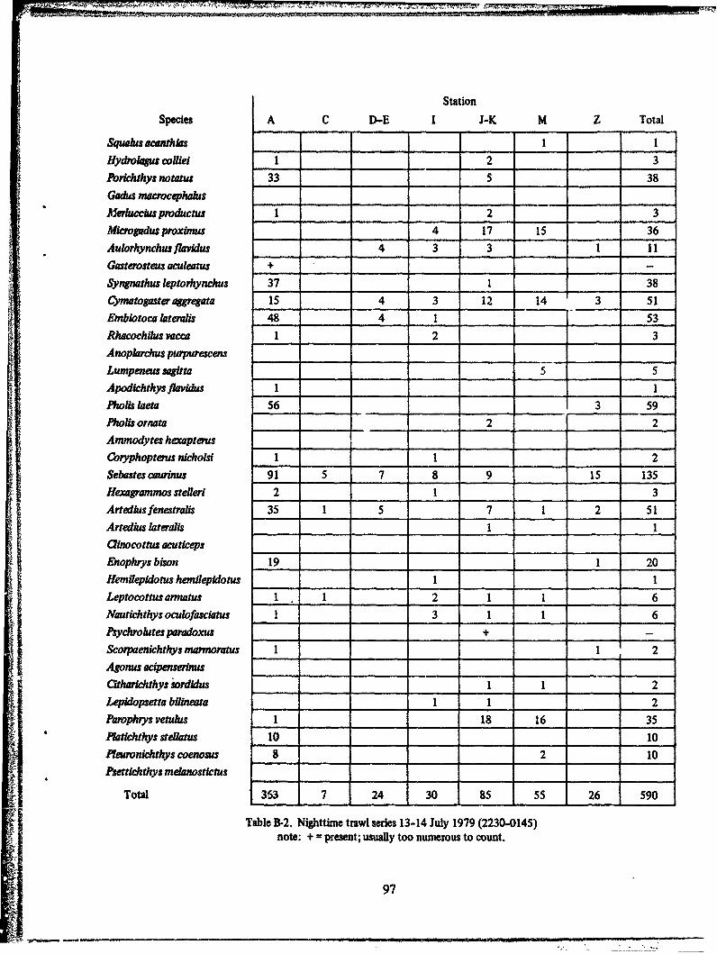
Station

species A C D-.E I i-K M Z Total

Squahas awinthlas I_______

Hydrolagua colUel 1 _ __ _ _ __2 _ _ _ _ _ __ 3

Porkchthys notatus 33 _ __ ________ 5 _ __ __ 38

Gahas macrocephakis __ ____ ____

MIduchs productus 1 2 3Mkrogadus proxlmu 4 17 15 36Aulorhynchus fiavidus ___ ___ 4 3 3 1 11

Gaserosteus aculatus + _ __ ________

Syngnathus leptorhynchu 37 ___________ 1 38

Cymatogasteraggrgat 15 4 3 12 14 3 51Embiotoca laterolis 48 ___ 4 1 53Rhacochilus vacca 1 _ __ 2 _ __ ___ 3

AnopLarchs pwpurescens ______ __

Lumpeneus aatta ____ _______ ________5 _ ___ 5

Apodichthys flavWdu 1 I__________ _ _ _ _ _ _ ___

r Phollslamt 56 _ _ _ _______ 3 .59Pholis ornata____ ___ 2 _ __ ___ 2

Amtmodytes hexapterus _________ __ __

Coryphopterus nicholsi 1 1 2Sebastes caurmnus 91 5 7 8 9 15 135Hexagnuamos steiled 2 ____ ____ 1 ___ 3

Art edhis fen est rais 35__ 1_ _ 5_ _ 7_ _ 1_ _ 2_ _ 51_

Arteduisiateraiis I_ I_ _ _ _ _ _ _

Enophrys bison 19 ____ ____ ___ ___ _ _ _ 120Hemilepidotus hemilepldotus I_______ ___

Leptocottsarmatus -1, __ 2 1 1 ___ 6-Nautichthys oculofasciats 1 ____ ____ 3 1 1 _ __ 6Psychrolutes paradoxu _ __ _ _ + __ _ _ _ _ _

corpaenlchthys martmoratus 1I____________ ___ 1 2

Agomis acienserhnus _____

atharichthyj sordidus 1 1 ____ 2

Lepidopsetta bfilieaia 1 1 ____ ___ 2Parophrys Yetduhn 1 ____ 18 16 ____ 35Platichthys stellaus 10 ____ _ _ _ _ _ _ 10fleuronicihys coenosus 8 ___ ___ 2 10?settichthys melanostictus____________

Total 363 7 24 30 85 55 26 590

Table &-2. Nighttime trawl series 13-14 July 1979 (2230-0145)

note: + = present; usually too numerous to count.

97

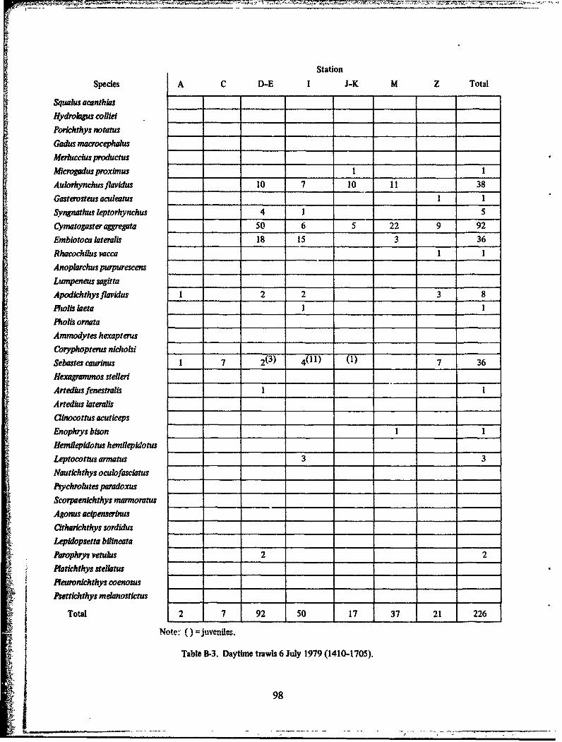
Station

Species A C D-E I i-K M Z Total

Squalus acanthias ____ ____

Hydrolazs collie!_ _ _ _ _ _ _ _ _ _

Porchthys notatus________

Gadus macrocephalus ____ ___

Merluccius productus ___ ____

Microgadus proxinus I__ I___

Aulorhynchus fiavidus ___ ___ 10 7 10 11 38

Gasterosteus aculeatus 1 1

Syngnahus leptorhynchus _ ______ 4 1 5

Cymatogaster aggreta _ ______ 50 6 5 22 9 92

Embiotoca lateralis _ ___ 18 15 3 36

Rhacochilus vacca 1 IAnoplarciws pwpwuescens ___ ___

Lumpeneus sagitta ______ ___ ___

Apodichthys flavidus 1 ____ 2 2 3 8

Phofs laeta I_ _ I_ _ _ _ _ 1_ _ _ _ _ _ _ _

Phais ornata__ __ ____

Ammodytes hexaptemls____

Coryphoptenis nichols! __ ___ ___

Sebastes caurinus 1 7 2(3) 4011) (1) 7 36

Hexagram os stelleri_ _ _ _ _ _ _ _ _ _____ _ _ ___

Artedius feneshuls I__ I___

Artedius laterali, _ _ _ _ _ _ __ _ _ _ _ _ _

atnocotw..s acuticeps_____ ______ ______ _____

Enophyys bison I_______ _____ ____ ___

Hemilepidotus hemilepidotus ________ ____ ________ ____

Leptocottus armatus 3 3Nautlchthys oculofasciatus _ _ _ _ _ _ _ _ _ _ _

hsychrolutes paradoxus______ __________

&corpenlchthys mamnoratus ____ ___ ______

Agonus acipenserinus _ _ _ _

Cftharlchthys sordids___ ____ ___ ___

Lepidopseta bilincata _ _ ________ ___

Parophrys vetulus 2 2Pflatchthys stellatus_____ _____ __ ______ ____

Pfeuronlchthys coenosus ___ _ _ _ ____ _ _ _ _ ___

Psettichthys melanostictus _ _ _ _ _ _ _ _ _ _

Total 2 7 92 50 17 37 21 226

Note: (= juveniles.

Table B-3. Daytime trawls 6 July 1979 (1410-1705).

98

Station

Species A C D-E I i-K M Z Total

Squalus acanthias 1 1

Hydrolgus collie!____ 2 2

Porichthys notatus 1 I___

Gadus macrocephalus ____

* ~~Merluccius productus ____

Microgadus proxinius ____1 4 5

Aulorhynchus flvidus 2 1 22 25Gaa-erosteus aculeatusSyngnathus leptorhynchus ___ ___ ___

Cymatogaster aggregta _ ______ 1 1 24

Embiotoca lateralis _ _ __ _ _ _ _ _ _ _ _ _ _ _

Rhacochilus vacca 1 1

Anoplarchus purpurescens __ _ __ _ __ __ _ __ _ _ _ _ _ _

Lwmpeneus sagtta _ ___1 12 13

Apodichthysflavidus__ _ _ _ __ _ __ _ _ _

Pholis laeta 3 _ __ ___ 3

* Pholis ornata ____ ____ 1 1 2

Amtmodytes hexapteru _ _ __ _ _ _ ______ _ _

Coryphopterus nicholsi___ _______ ___ ___ ___

Sebastes cturinus 28 4 9 _ __ (2) 14 57Hexagrammios stellen _______________ _________

Artedwis fenestndis_ _ __ _ _ _ _ __ _ _

Artedius lateralis _ __1 __ _ _ 1 2

afrocottus acuticeps __ _ _ _ _ _ _ 4 4

Enophrys bison I I___ ________ ___

Hiemulepidotus hemilepidotus ___ ___ ___ ___

Leptocott us arnnatus 2 ___ ____ __ ___ ___ 2

Nautichthys oculofasciatus 1 1

hsychrolutes paradoxus ____5 10 29 44

Scorpaenichthys mannoratus _______ ____________

Agonuis acipenhrus _ _ ___ _ _ __ _ _ __ _ _ _

citharichthys sordidus 2 3 7 3 15Lepidopsetta bitineata _ _______ 6 2 1 9

Parophrys vetulus 1 3 2 2 10 30 48

Platichthys steilatus I_ _ I___ _ _ _

Pleuronichthys coenosus 2 2

Psettlchthys melanos~tichs _ _ _ _ _ _ _ _ _ _ _

Total 41 9 12 25 31 109 16 243

Note: ()=juveniles.

Table B-4. Nighttime trawl series 24-25 June 1980 (2130-0115).

99

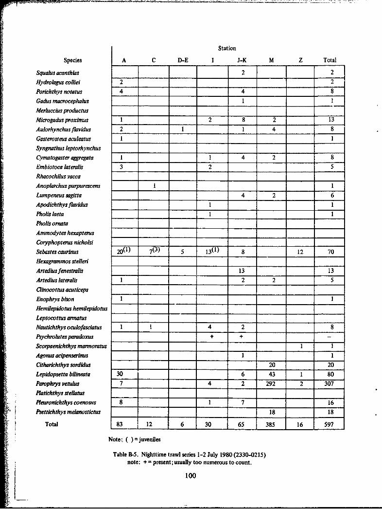
Station

Species A C D-E I J-K M Z Total

Squalus acanthias 2 2

Hydrolagus colliei 2 12Porichthys notatus 4 4 8

Gadus macrocephalus I___ I____

Merluccius productus

Microgadus proximus 1 2 8 2 13

Aulorhynchus flavidus 2 1 1 4 8

Gasterosteus aculeatus 1 1

Syngnathus leptorhynchus_____________

Cymatogaster aggegata 1 1 4 2 8

Embiotoca lateralis 3 2 5

Rhacochilus vacca

Anoplarchus purpurescens 1I

Luinpeneus sagitta ____ ____ 4 2 6

Apodichthys flavidus IPholis laeta I________

Pholis ornata

Ammodytes hexpterus _________ _________

Corj'phopterus nicholsi 8____ 12___ 70__ ___

Sebastes caurinus 20(1) 7(3) 5 1318127

Hexagrammos stellera ___ ____

Artediusfenestrulis __ _ ___ 13 13

Artedius lateralis 1 ____ ___ ____ 2 2 5

aanowrmts acuticepsEnophrys bison I 1

Hemilepidotus hemilepidotus___ _____________

Leptocottus anntus ___________________ ___

Nautichthys ocubofasciatus 1 1 4 2 8

Psychrolutes paradoxus + +

Scorpaenichthys marmoratus 1 1

Agonus acipenserinus I___ I___

Citharichthys sordidus _________ 20 20

Lepidopsetta bifineata 30 6 43 1 80Parophry Yetulus 7 4 2 292 2 307Pbatichthys stellatus___ ___ _______ ___

Pleuronachthys coenosus 8 1 7 16Psetttchthys melanosticus _ ___ ____ 18 18

Toal8 ~ 26 30 65 385 16 59

4.Note.-, )=juveniles

Table B-5. Nighttime trawl series 1-2 July 1980 (2330-0215)note: + =present; usually too numerous to count.

100

Station

Species A C D-E I J-K M Z Total

Squalus acan~hias I___ ____ ____ 1 ____

Hydrolagus cofliel ____ 2 ____ ____ 3 5

Porichthys notatus_____ ____ ____

Gadus rnacrocephalus _ _ __ _ __ _ _

I. ___ ___ ____ ___u

Microgadus proximus ____ ____2 2

Cymtatogaster aggregata _ __ 1 ___ 2 _____ 3

Embiotoca lateralis _________

Rhacochilus vacca 11Anoplarchus purpurescens 11

Lumpeneus sagitta ________

Apodichthys flavidus_________ ____

Pholis laeta_____ ____ ____ _____

Pholis ornata___ __ ____

Ammodytes hexaptemus ___ __

Coryphopterus nicholsi ________

Sebastes caurinus 11 9 _ __ 2 _____22

Hexagrammos stelleri_____________

Artedius fenestralis I 1

Artedius kit eralisCinocottus acuticeps___ _________

Enophrys bison___ ______

Hemilepido has hemilepidotus ________ __ _ ________ ____

Leptocottus armatus 1 1

Nautichthys ocudofasciatus________

Psychroiutes paradoxus ___ ___ ____ ___ ___ ___

Scorpaenichthys marmoratus 1I ___ ________ ____ ________

Agonus acipenseinus_____ ____

Citharichthys sordidus __ ______ _____ 3 3________

Lepidopsetta bilmneata 1 1 8 10

Parophrys vetulus 3 14 1 18Platichthys stellatus ____

Pleuronichthys coenosus11* ~~Pseffichthys melanostictus ____ ________ ________ ________

Total 14 5 11 09 31 1 71

Table B-6. Nighttime trawls 28-29 May 1981 (2230-0130).

101

Species A C D-E I SainJ-K M Z Total

Squalus acanthias - ___

Hydrolagus cofllie_ _ _ ___ ____ _ _

Porichthys notatus ____ ___________

Gadus macrocephalus_____ ________

Merluccius productus ____ ___

Microgadus proximus ___

Aulorhynchus flavidus ___ ___ ____ ____

Gasterosteus aculeatus____

Syngnathus leptorhynchus I______

Cymzatogaster aggregta ____ 4 15 19

Embiotoca lateralis 8 8

Rhacochilus vacca

Anoplarchus purpurescens ____ ________

Lunipeneus sagitta_________

Apodichthys flavidus

Pholis Ia eta__________ _____ ___ _ _____

Pholis ornata ___ 2 2

Ammodytes hexaptenms I 1

Coryphopterus nicholsi_______ ___ __ __ ____ ____

Sebastes caurinus 4 4 4 12

Hexagrammos stelleri_____ ________

Artedius fenestralis 2 2

Artedius lateralis _ _ _ _ _ _ _ _ _ _ _

Clinocottus acuticepsj

Enophrys bison_______________ ______

Hemilepidotus hemilepidotus ______ __ ___________

Leptocottus annatus11

Nautichthys oculofasciatus________________ ____

Psychrolutes paradoxus____ __________ __ ____ ____

Scorpaenichthys inannoratus ________ ___ ___

Agonus acipenserinus ____ ____________

Citharichthys sordidus-

Lepidopsetta bilineata______ _______ 11

Parophrys ve*tulus 1___ 1 ____L 2

Platichthys stellatus ____ ____ ________

Pleurornihthys coenosus________

Psettichthys melanostictus ____ _________ _________ ____

Total F8 _ _ 35 _ _ _ _ E4

Table B-7, Nighttime trawls 5 June 198:' 0330-0530 (stat ions Z, C and I only sampled)..

102

APPENDIX C

OYSTER MANAGEMENT PLAN

103

NAVAL SUBMARINE BASE, BANGORFIVE YEAR MANAGEMENT PLAN FOR THE

PACIFIC OYSTER, Crassostrea gigas(FY82 to FY87)

I. INTRODUCTION

A. Objective:-

The objective of this plan is to produce a managed oyster resource which willprovide recreational opportunities to SUBASE personnel and dependents. It will also pro-vide a means for commercial harvest of the excess resource which is surplus to the needs ofrecreational activity,

B. Background:

Between June 18 and July 2, 1981 beaches containing the Pacific oyster, Crasso-

strea gigas, along SUBASE, Bangor were surveyed for quantity and density of oysters (figureC-1). This information, along with a proposed management plan for the resource was pre-sented to the Commanding Officer SUBASE on 27 August 1981. This meeting resulted inthe management plan presented below.

II. SURVEY METHODS

Beaches with obvious oyster beds were chosen for survey. The beds were measured for

length and every 30 meters a bed width was recorded. At every width site samples weretaken at top, middle and bottom by a random toss of 0.1 M2 (I ft2 ) ring. Oysters within thering were sorted into those greater than 3 inches in length and those 3 inches or less in length,

and counted. (The 3 inch criteria was chosen because it represents commercial desirabilityand SUBASE requires a 3 inch minimum length for recreational harvest.) The area, averagedensity, and number of oysters in each bed were then calculated.

III. SURVEY RESULTS

Table C-i summarizes the survey results by beach. Beach numbers refer to oyster bedsindicated in figure C-1. Beaches 3 and 4 contain large numbers of commercial size oysters.Oyster densities on commercial beds are generally regulated to yield 1,000 to 1,500 bushelsper acre. Beaches 3 and 4 contain 9,900 and 13,500 bushels per acre respectively of com-mercial size oysters. One bushel of adult sized oysters contain 80 to 125 oysters and will

yield about 8 pints of shucked meats.

IV. MANAGEMENT PLAN

Table C-2 is a summary of the Five Year Oyster Resource Management Plan.

104

Number

Area Average Oysters Number Oysters NumberBeach Number in Density Total Number Less than 3" and Greater Limits(Beach Name) Acres (ft2 ) Oysters 3" in Length in Length (3" and Larger)

1. Cattail Beach(a) 0.27 13.3 158,000 34,000 124,000 6,900(b) 0.17 13.1 95,000 20,000 75,000 4,200(c) 0.04 8.5 14,000 3,000 11,000 600(d) 0.46 19.2 385,000 96,000 289,000 16,000

2. Tang Beach(a) 1.8 12.3 962,000 297,000 665,000 37,000(b) 0.13 7 40,000 17,000 23,000 1,300

3. Carlson Cove 1.8 34 2,559,000 602,000 1,957,000 109,000

4. Carlson-South 2.4 42 4,428,000 1,223,000 3,205,000 178,000

5., Devils Delta & EHW Beach(a) 0.7 9.4 270,000 69,000 201,000 11,000(b) 0.09 14.3 58,000 24,000 34,000 1,900(c) 0.13 21 118,000 14,000 104,000 5,800(d) 0.07 46 138,000 27,000 111,000 6,200(e) 0.14 13 79,000 18,000 61,000 3,400(M) 0.3 17.8 234,000 42,000 192,000 10,700(g) 0.11 42.4 202,000 32,000 170,000 9,400(h) 0.18 14 110,000 25,000 85,000 4,700

TOTALS 8.79 9,850,000 2,543,000 7,307,000 406,100

Table C-I, Summary of 1981 oyster survey: Naval Submarine Base Bangor.

1

105

IN

/10

A. Recreational Shell Fishing

The management plan was developed to provide adequate recreational harvest forSUBASE personnel with a projected annual harvest of 20,000 limits at 18 oysters per limitper year. The projected limits are higher than records indicate for past years, and perhapswill not be attained in the initial year- of this plan. This management plan will be amendedeach year to reflect actual recreational harvest experience. Harvest rates are expected to in-crease with the increase in Base population in the next several years.

Beaches will be utilized, in most cases, for both clam and oyster sport fishing andin some cases, such as Beaches 3 and 4 where dense concentration of oysters exist, only alimited area of beach should be opened at any one time during the recreational harvestperiod. Strip harvesting is recommended on these beaches because clam diggers may tram-ple the oyster beds in search of clams. Opening small sections of the beach to oyster andclam harvest will eliminate much of the wastage that could occur if the entire beach wereaccessible,

B. Commercial Harvest

Beaches 4 and 5 will be opened to commercial permit harvest during FY 82.Beach 4 contains the highest density of oysters and is extremely overcrowded. Beach 5is planned for harvesting in FY82 because of anticipated tightened security in future years.Beach 3 will be opened for commercial fishing in FY83, in order to harvest an estimated2.3 million oysters remaining after the recreation take in FY82., No additional commercialharvesting is anticipated until FY86, and would take place at Beach 4 after the recreationalharvest of FY85 (table C-2). Commercial harvesting will take place during winter or earlyspring, depending upon oyster condition, marketing and the permittees' schedule..

C. Reseeding

A portion of the monies generated from the commercial harvest will be used toreseed beaches that have been harvested or contain small populations of oysters. Reseedingwill only be done at Beaches 1, 2, 3, and 4 as it is expected that tightened security at Beach5 will preclude recreational or commercial use of this area. Seeding will take place in Aprilor May of each year in order to take advantage of the spring and summer period of optimumgrowth conditions. Reseeded beaches will be opened for harvesting at two and one half yearintervals, depending upon growth rate.,

D. Management Plan Revision

Shellfish populations are dynamic and subject to changes such as growth, harvest,and depredation. Management priorities and security requirements are also dynamic. Theharvest schedule presented in table C-2 will be revised at the intervals necessary to reflectchanges in populations or priorities, and to reflect the success of new programs such as oysterseeding and commercial harvest.

107

FY 1982 1983 1984 1985 1986

ActionItem ON DJ FM AM JJAS ONDIFMAMJ IAS 0 N DJ F M A MJ J AAS 0 N DOJ F M A MJ JAS ON DI FMAMJJAS

1. Open Beach 3 forrecretionallfshing R R RRRRR RRR R R R R RRR I R RR

2. Prepare and awardcommercial harvestpermit XXX X XX

3. Commercial har-vest Beaches4aand CC C C c C C C

(Beach 4)

4. Reseed Beach 4 SS SS

S. Open Beach 2 forecreationalfishing R R RRRRRRRRR

6. Prepare and awardcommercial harvestpermit X X

7. Commercialharvest Beach 3 CC C

8. Reseed Beach 3 S S

9. Open Beach 1 forrecreational fashing R RR RRR R R R RR

10 Reseed each 2 S S

11. Open Beach 4 forrecreational shell-fishing It R R R RR R R R RR

12. ReseedBeach I S S

Note Washington State Regulationsprohibit recreational oyster harvestbetween July 15 and September 15

Table C-2. Five-year oyster resource management plan.

11 108

"APPENDIX D

BIVALVE MOLLUSC I ENGTH-FREQUENCY DISTRIBUTICNS

10

•l 109

Bivalve length-frequency distribution data collected at SUBASE Bangor durin~g 1979,

1980 and 181 surveys are presented in figures D-1 through D-4 for Saxidomus giganteus,

Protothaca staminea, Tapes japonica and Clinocardium nuttallfi, respectively.

110

TRIDENT IX, X & XISaxidomus giganteus

1979

0

'U

0

~30-

20,

10,

20-

1980

z S10-

, I * I *

20-

1981z io-

01

10 20 30 40 so so 70 80 90 100

LENGTH (mm)

111

100- TRIDENT IX, X & XIProtothSca staminea

90.

so- 1979

70"

60.

2o

0

40-

w

20-

10-

hL

--

30-

1980

120

30

30

1912

£L 10"

LENGTH (mmr)

TRIDENT IX, X & XITapes Japonica

20-

1979

S10o1o

0

.z 1980

z

11

0

U

0

0 20 30 40 50 60 70

LENGTH (mm)

_ 113

APPENDIX E

SELECTED IMPORTANT SPECIES

P 6AMK-XU~W UUl

115

'Z.

COPPER ROCKFISHSebastes caurinus Richardson, 1845

4, .-

464

RED ROCK CRAB

Cancer productus Randall, 1839

116

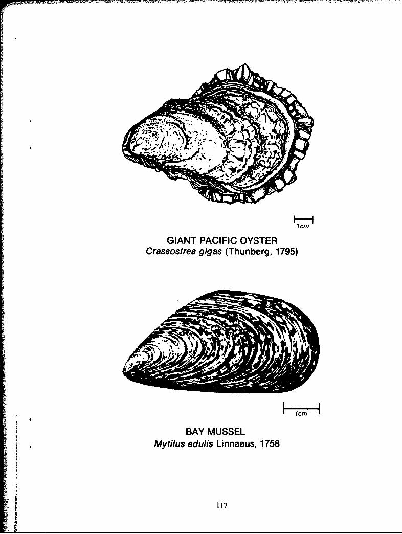
1cm

GIANT PACIFIC OYSTERCrassostrea gigas (Thunberg, 1795)

BAY MUSSEL

Mytilus edulis Linnaeus, 1758

1 117

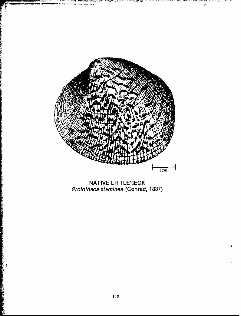
1cm

NATIVE LITTLENECK

Protothaca staminea (Conrad, 1837)

118

BUTTER CLAMSaxidomus gigan teus (Desh ayes, 1839)

1cm

MANILA LITTLENECKTapes japonica Deshayes, 1853

j 119

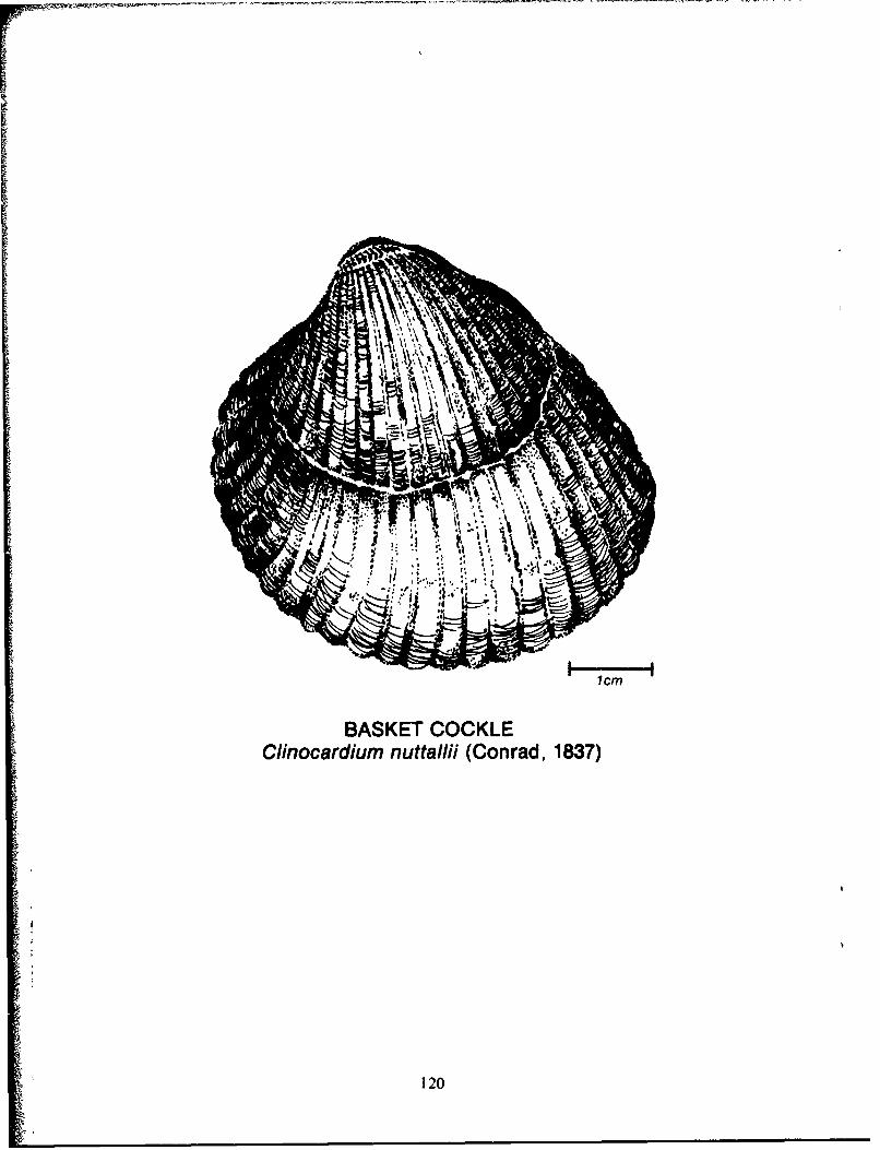
lcm

BASKET COCKLEClinocardium nuttallil (Conrad, 1837)

120

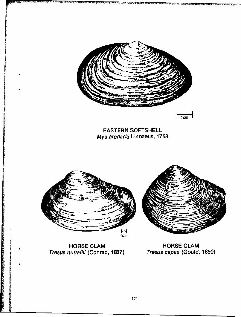
EASTERN SOFTSHELL

Mya arenaria Linnaeus, 1758

1cm

*HORSE CLAM HORSE CLAMTresus nuttaillii (Conrad, 1837) Tresus capax (Gould, 1850)

121

Er I 4v

1cm

GEODUCKPano pea generosa (Gould, 1850)

122

mop,

The Copper rockfish is a common species which inhabits both eelgrass-laminarian-sargassum and piling habitats along SUBASE Bangor. Its geographic range extends fromMonterey Bay, California tc the Gulf of Alaska. The copper rockfish possesses dark fins, adark brown to olive coloration on the upper body, blotched coppery coloration laterally,and a deep caudal peduncle. This species bears its young alive, usually during June and Julyadjacent to SUBASE Bangor. Primary food items for this species include shrimp, fishes,worms and miscellaneous other crustaceans such as amphipods, crabs and isopods. Copperrockfish are prized for human consumption in Puget Sound and have been observed to weighup to 5 kg in Hood Canal. This species has been used for heavy metal monitoring (muscleand liver tissue) and extensive food habit observations during SUBASE Bangor environmen-tal investigations.

The red rock crab is common subtidally along SUBASE Bangor waterfront areas,especially adjacent to piers and pilings. Its geographic distribution extends from MagdelenaBay, Baja California to Kodiak Island. The red rock crab can be recognized from the dunge-ness crab by its dark red upper carapace surface and yellowish underside with red-orangeblotches. The tips of the large claws are black-tipped., Red rock crabs have an extendedbreeding season in Hood Canal from spring through late summer. While less desirable forhuman consumption than the dungeness crab, red rock crabs are often collected intertidallyalong SUBASE Bangor by sports clam harvesters. This species is being used for heavy metalmonitoring during ongoing environmental studies at SUBASE Bangor.

The Pacific (or Japanese) oyster population inhabiting the SUBASE Bangor water-front areas presently consists of extensive intertidal beds along most open beaches (seeappendix C). An excellent oyster spatfall occurred durir. several recent years (1978-1980)throughout northern Hood Canal waters. This species occurs from Morro Bay, California toBritish Columbia. The pacific oyster was introduced from Japan during the 1920-1930period. A commercial oyster industry exists in several regions of Puget Sound. Oysters inHood Canal usually spawn during July and August when water temperatures are favorablywarm (usually about 67 degrees Farenheit). For normal growth of oyster larvae during thefast several weeks of existence, water temperatures above 68 degrees F are required., Adultpacific oysters will reach lengths in excess of 30 cm. This species also is being used for heavymetal monitoring at SUBASE Bangor during environmental studies.

123

The bay mussel (or blue mussel) inhabits pilings and floating structurer ,SUBASE Bangor waterfront areas. This cosmopolitan species is distributed worldwide insheltered bays and estuaries. Bay mt,%els form dense aggregations on pilings and are impor-tant members of the food web in Ho-od Canal. While cultured in Europe and on the east coastfor human consumption, this spocies has only recently been utilized on the Pacific Coast forother than fishing bait. Spawning occurs in spring and early summer in Puget Sound. Thisspecies has been used for heavy metal monitoring at SUBASE Bangor. An extensive amountof literature exists for ths species as a test organism for environmental monitoring studies.

The native lictleneck (or steamer) clam is abundant intertidally along SUBASEBangor beaches. This species occurs from lower California to the Aleutian Islands. Spawningoccurs in late spring and early summer in Hood Canal. Native littleneck clams occur higherintertidally than butter clams and shallower (about 3-5 cm deep) in the substratum. Thisspecies is densest in cobble beac, 'iabitat3. Native litttleneck clams are usually more roundin shape and white in coloration than the Manila or Japanese littleneck clam. This species ishighly esteemed for human consumption in Puget Sound and elsewhere. Native littleneckclams were the most numerically dominant clam species during SUBASE Bangor environ-mental investigations.

The Manila (or Japanese) littleneck clam is abundant on some beaches ?Jong SUBASEBa-gor. This species is usually more elongate than the native littleneck clam. The Manilalittleneck clam often has intricate geometric patterns on the shel!. Its geographic distribu-tion ranges from Elkhorn Slough, California to British Columbia. This species was introducedwith Japanese seed oysters during the 1920-1930 period. Spawning of Manila littleneckclams occurs from May-October, with a peak in July for Hood Canal waters. This species isoften collected along with native littleneck clams for "steaming" and is an excellent foodclam in Puget Sound.

The butter clam is abundant along SUBASE Bangor intertidal regions. Its geographicrange occurs from northern California to the Aleutian Islands. This species is the most im-portant commercial clam species in Puget Sound. Butter clams attain a relatively large adulisize (commonly 80-100 mm in length). Butter clams are excellent for human consumption,usually being fried or used for chowder., This species spawns in Hood Canal during April toOctober. Juvenile butter clams and siphon tips of adults are important diet items for manyHr,o( Canal fishes. This species represented the greatest biomass of bivalves sampled duringSUBASE Bangor environmental studies. This species will be used for heavy metal monitor-ing beginning wit. the 1982 survey.

Basket cockles are common along some SUBASE Bangor beaches, usually inhabitingthe gently sloping, delta regions in the sand and eelgrass habitat. Its geographic distributionranges from San Diego, California io the Bering Sea. Spawning usually occurs during mid-summer (July-August) in Hood Canal for this hermaphroditic bivalve species. Basket cocklesare tasty, excellent food clams; however, adults of this species arc quite tough when cookedunless thay are chopped or ground into chowder. Juveniles of this species are a major foodsource for many Hood Canal fish species.

124

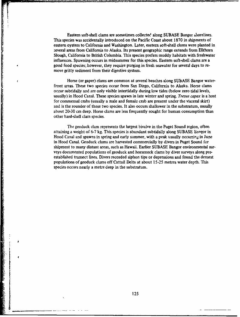
Eastern soft-shell clams are sometimes collectece along SUBASE Bangor sjhorelines.This species was accidentally introduced on the Pacific Coast about 1870 in shipments ofeastern oysters to California and Washington. Later, eastern soft-shell clams were planted inseveral areas from California to Alaska. Its present geographic range extends from ElkhornSlough, California to British Columbia. This species prefers muddy habitats with freshwaterinfluences. Spawning occurs in midsummer for this species. Eastern soft-shell clams are agood food species; however, they require purging in fresh seawater for several days to re-move gritty sediment from their digestive system.

Horse (or gaper) clams are common at several beaches along SUBASE Bangor water-front areas. These two species occur from San Diego, California to Alaska. Horse clamsoccur subtidally and are only visible intertidally during low tides (below zero tidal levels,usually) in Hood Canal. These species spawn in late winter and spring. Tresus capax is a hostfor commensal crabs (usually a male and female crab are present under the visceral skirt)and is the rounder of these two species. It also occurs shallower in the substratum, usuallyabout 20-30 cm deep. Horse clams are less frequently sought for human consumption thanother hard-shell clam species.

The geoduck clam represents the largest bivalve in the Puget Sound region, oftenattaining a weight of 6-7 kg. This species is abundant subtidally along SUBASE Barigor inHood Canal and spawns in spring and early summer, with a peak usually occurring in Junein Hood Canal. Geoduck clams are harvested commercially by divers in Puget Sound forshipment to many distant areas, such as Hawaii. Earlier SUBASE Bangor environmental sur-veys documented populations of geoduck and horseneck clams by diver surveys along pre-established transect lines. Divers recorded siphon tips or depressions and found the densestpopulations of geoduck clams off Cattail Delta at about 15-25 metres water depth. Thisspecies occurs nearly a metre deep in the substratum.

125

APPENDIX F

TAXONOMIC CHECKLIST ADDITIONS

127

Additions to the SUBASE Bangor cumulative checklist of organisms collected fromHood Canal are listed in table F-1. Reference specimens of these taxa are maintained at theNOSC sample processing center located at the Hawaii Laboratory.

128

TAXA

CNIDARIA

HydrozoaObelia plicata Hincks, 1868Clytia edwardsi (Nutting, 1901)Euphysa flammea (Lincko, 1905)

AnthozoaAnthopleura art emisia (Pickering in Dana, 1948)

NEMERTEACayinonta mutabiis Griffin, 1898

ENTOPROCTA

Barentsia ramosa (Robertson, 1900)

ECTOPROCTA

Schizoporella unicornis (Johnson, 1847)

ANNELIDA

Pectinaria granulata (Lmnnaeus, 1767)

ARTHROPODA

IsopodaGnorimosphaeroma oregonensis (Dana, 1854)

CaprellideaMetacaprella anomala (Mayer, 1903)

GamnmarideaPontogenia intermnedia Gurjanova, 1938

DecapodaPagurus hirsutiusculus (Dana, 185 1)Pinnixia occidentalis Rathbun, 1893Pinnixia tubicola Holmes, 1895

ECHINODERMATA

Amphodia occidentalis (Lyman, 1860)

CHORDATA

BatrachoididaePorichthys notatus Girard, 1854

GadidaeGadus macrocephalus Tilesius, 18 10

CottidaeArtedius lateralis (Girard, 1854)

AgonidaeAgonus acipenserinus Tilesius, 1811

BothidacClrharichthys sordidus (Girard, 1854)

Table F-1, Additions to the SUBASE Bangor cumulative checklist.

129