This project has received funding from the European Union Horizon 2020 Research and Innovation action under grant agreement No 822781

Working Paper

Patterns of growth in structuralist models: the role of the real exchange rate and industrial policy Gabriel PorcileEconomic Affairs Officer, ECLAC and UFPR

Danilo SpinolaUnited Nations University (UNU-MERIT) and Maastricht University

Giuliano Yajima Department of Social Sciences and Economics, Sapienza University of Rome

15/2020 June

1

PATTERNS OF GROWTH IN STRUCTURALIST MODELS: THE ROLE OF THE REAL EXCHANGE RATE AND

INDUSTRIAL POLICY

Gabriel Porcile1; Danilo Spinola2; Giuliano Yajima3

This paper presents a Balance-of-payments (BOP)-constrained growth model in which the

interaction between the real exchange rate (RER) policy and industrial policy result in the

emergence of different patterns of growth and income distribution. The paper relies on

cumulative causation à la Kaldor and path-dependency to relate both types of policies. The

transition from one equilibrium level of the RER to a new equilibrium level generates a process

of learning that transforms the income elasticity of exports and hence the BOP-constrained rate

of growth in the long run. The model produces a variety of outcomes that help explain the

contradictory results that emerge from the empirical literature on the impact of the real

exchange rate on economic growth in the long run.

Keywords: Real Exchange Rage; Structural Change, Growth models, Structuralist models, BOP-

constrained growth.

JEL: O33, O40, O41

1 Economic Affairs Officer, ECLAC and UFPR. jose.porcile@cepal.org 2 United Nations University (UNU-MERIT) and Maastricht University. sartorello@merit.unu.edu 3 Department of Social Sciences and Economics, Sapienza University of Rome. giuliano.yajima@uniroma1.it

2

PATTERNS OF GROWTH IN STRUCTURALIST MODELS: THE ROLE OF THE REAL

EXCHANGE RATE AND INDUSTRIAL POLICY

1. Introduction

Structuralist models take into account the specific role that different institutional

settings, power relations and economic structures play in shaping economic outcomes4. This

paper presents a model in which the interactions between structures, power and institutions

result in the emergence of different patterns of growth and income distribution in peripheral

economies. The structural dimension is captured by the country’s pattern of international

specialization, expressed in the income elasticity of exports and imports. The institutional

dimension is captured by what Nelson and Sampat (2001) call “social technologies” which

represent (implicit or explicit) forms of coordination widely accepted by and incorporated to

the behaviour of public and private socioeconomic actors. Our focus is on institutions governing

technical change and the behaviour of the real exchange rate. For simplicity, we will refer to

them as “industrial policy” and “exchange rate policy”, although they involve complex

interactions among workers, capitalists and governments.

The key mechanism that relates policies to structures is learning by doing. Under certain

conditions (discussed in the paper), the depreciation of the real exchange rate (RER) stimulates

economic growth and investment, leading to the accumulation of knowledge, which in turn

redefines the income elasticity of exports. The model thus entails a process of “deep path-

dependence” as defined by Setterfield and Cornwall (2002), in the sense that its parameters

change as the economy moves towards its long-run equilibrium, after a shock produced by the

depreciation of the RER.

The modelling strategy combines a Neo-Kaleckian approach to investment and income

distribution with a Balance-of-Payments (BOP) constraint on growth5. We assume a centre-

periphery system, in which the centre is the technological leader and the periphery is

specialized in sectors with lower income-elasticity of exports than the centre. The challenge of

the periphery is to transform its pattern of specialization using the exchange rate and industrial

policies. The paper presents three scenarios for the periphery that we consider representative

of different combinations of these policies, which in turn reflect different power relations

among three actors (the government, capitalists and workers). Each scenario is a stylized

representation of growth patterns effectively observed in different countries or even in the

same country at different points in time.

4 See Taylor (2004, p.3). 5 The combination of Kaleckian and Thirlwallian features can be found in Dutt (1992). This model is an inspiration,

but our model proposes rather different closure equations.

3

The first scenario is the “developmentalist state” (presented in section 3) in which the

government aims at a competitive exchange rate while implementing a strong industrial policy

to foster learning and structural change. The policy focus is on international competitiveness,

and there is in power an “industrialist coalition” whose objective is to maximize the investment

rate and close the technology gap with the technological leaders.

The second is the “heterogeneous preferences” scenario (section 4) in which there are

contending forces over the RER which reflect the different objectives of governments,

capitalists and workers. The RER endogenously responds to political conflict among domestic

actors, probably in association with the alternation of power between centre-right and centre-

left political coalitions in democracy. Various potential outcomes from this scenario are

considered, and their implications for growth and distribution analysed.

The last scenario (section 5) is called “financialization”. The RER fluctuates out of the

interaction between a government that uses monetary policy to control inflation, and

international capital flows that arbitrate between the rates of return of assets denominated in

different currencies. This scenario corresponds to a model in which there is a “neoliberal

coalition” in power that focuses solely on curbing inflation while keeping the capital account

fully open. The openness of the capital account implies that capitalists and workers have little

direct influence over the RER, which is driven by shocks in the international financial markets.

Two caveats are necessary. First, in all cases we assume that technical change affects both

productivity growth (and hence price competitiveness) and the pattern of specialization

(reflected in the income elasticity of exports). Both effects are contemplated, but the main

focus is on changes in the income elasticity of exports. Second, the institutional and political

conditions are considered given in the model, which allows us to concentrate on the

macroeconomic outcomes of each scenario.

2. Review of the literature on RER and Growth

Review of the empirical literature

The role of the exchange rate and industrial policies is at the core of the current debate

on growth, structural change and income distribution in developing economies. This is so

because of its role in the determination of prices and ultimately incomes levels, much like

others nominal variables such as the wage and profit rates. In fact, the RER can count as both a

cost for some agents – such as firms, who for instance might see their earnings reduced

following a fall in the RER - and a component of revenue flows for others6- such as households,

who on the contrary might experience an increase in their purchasing power. Although this

6 For a recent review of ongoing debate on this topic see Medeiros (2020).

4

debate is far from new, it was revived after Rodrik (2008), who pointed out the existence of

RER level effects fostering the expansion of the tradable sector in developing economies.

According to his study, a depreciated RER stimulates changes in the composition of output

towards activities which are more dynamic from a technological standpoint, changing relative

prices in their favour. This change in output composition would trigger a second mechanism, a

sustained change in the level of output (that is, long run growth) as the economy as a whole

would experience increasing returns to scale.

This two-step mechanism (Rodrik, 2008) has been supported by a number of empirical

studies. Razmi et al. (2012), Rapetti et al (2012) and Ibarra & Blecker (2016) have provided

evidences of a positive effect of a depreciated RER on output growth. Currency devaluation

generates incentives for entrepreneurs in the tradable sector to invest via increased revenues

and profit margins, thus increasing capital accumulation. Conversely, a persistent overvaluation

of the RER would go in detriment of growth duration, as argued by Berg et al. (2012).

Moreover, Gabriel et al. (2020) have argued that undervaluation works better for higher level

of technological gap, as firms would compensate for their non-price competitiveness.

Eichengreen (2007) and Frenkel & Ros (2006) reinforce this story by finding a positive

association between a higher RER and a higher rate of employment growth, as a consequence

of the boost in capital accumulation.

Additionally, the empirical literature focusing on the effect of a depreciated RER on

structural change has provided some evidence of the positive causality pointed out by Rodrick.

However, authors diverge on how to measure and conceptualize structural change. Mcmillan et

al. (2014) see structural change as the “structural” component of increases in labour

productivity, caused by labour reallocation toward more productive sectors. Freund & Pierola

(2012) focus on the diversification of exported items and on the increase of the extensive

margin, while Cimoli et al. (2013) stress the technological intensity of exports. Marconi et al

(2016) suggest a positive effect of depreciation on the income elasticity ratio when the RER

approach an “industrial equilibrium” exchange rate7, hypothesis empirically tested by Missio et

al (2015) and by Nassif et al (2015), with data for Brazil.

In the two set of empirical works presented so far, positive effects RER depreciations

seems to prevail over the negative ones8. Price effects prevail over income effects, that is, an

increase in net export would overcompensate for the rises in external cost and the drop in real

7 The industrial equilibrium RER, as defined by Bresser-Pereira (2016), is the one that makes internationally competitive those industrial firms that are using state-of-the art technology. 8 The mechanism in which RER depreciations affect firms’ revenues, thus increasing internal funding and spending

in capital accumulation, is central in heterodox models along Kaleckian lines. Many heterodox works without a Kaleckian flavour highlight the structural change mechanism without discussing distributional changes (see Araujo & Lima (2007) and Araujo (2013)). Orthodox works state that the mechanism at play here is that currency devaluation corrects market and institutional failures thus acting as a second-best policy tool to promote economic

growth.

5

disposable income. This seems at odd with the “Kaldor’s Paradox”9 (Kaldor, 1978), in which

growth in unit labour costs has a positive correlation with growth in manufacturing export

share10. Nonetheless, there exist a number of contributions which point out toward a rejection

of Rodrick’s story, both at the theoretical and empirical level. For what concern the

depreciation-growth relationship, Diaz-Alejandro (1986) and Krugman and Taylor (1978) stands

out for being the most influential works expressing this exchange rate pessimism, a take

reprises more recently discussed by the theoretical works of Ribeiro et al (2016, 2017),

empirically discussed in Ribeiro et al. (2019). The theoretical standpoint of these works is that

an increase in RER would trigger inflationary pressure by raising the prices of imported capital

goods and reducing real wages, in this way dampening consumption and thus aggregate

demand. This can reduce economic growth and/or slowdown technical progress

Empirically, Nucci and Pozzolo (2001), investigating the relationship between RER

fluctuations and investment decisions with microeconomic data from Italy, support the idea

that exchange rate depreciation has a positive effect on investment through higher expected

revenues but a negative effect through higher costs. Caglayan and Demir (2019) find evidence

that the RER affects positively the expansion of low- or medium-skill manufactures, while skill-

intensive manufactures are less responsive. A similar conclusion is suggested by Agosin et al

(2012), by observing that export diversification does not improve following a RER depreciation.

Ribeiro et al. (2019) argue that, once functional income distribution and the relative level of

technological capabilities are explicitly considered, the direct impact of RER misalignments on

growth performance of developing countries becomes statistically non-significant. They suggest

that growth is explained mostly by technological capabilities and income distribution, as the

variable RER becomes statistically not significant when capabilities, income distribution and RER

are included separately in the regression. Finally, Ibarra and Blecker (2016), in their estimate of

the Balance-of-Payments-constrained rate of growth of Mexico, conclude that the impact of the

RER on exports is weak due to the high share of imported intermediate inputs in the total cost

of Mexican exporters11.

In recent years, the dynamic of the RER in developing economies has been shaped by

financial factors, mainly in form of currency volatility and rising external debt for the non-

financial sector. Procyclical capital inflows are behind the former, triggered by the boom in

commodity prices and by rising interest rate differentials – resulting from the implementation

of inflation targeting polies at the local level and the fall in global liquidity conditions. In turn,

change in the business behaviour of local exporting firms into financial intermediation activities 9 The Kaldor paradox highlights that countries excelling in manufacturing exports also exhibit higher unit labour costs precisely because higher exports induce higher productivity and hence higher real wages. Thus, policies

seeking to cut wages are unlikely to succeed in promoting exports and economic growth. 10 Boggio & Barbieri (2017) argues the relevance of testing not the rates of change, but the level effects of unit labor costs . 11 Similar results are reported for developed economies. Storm & Naastepad (2015), in turn, argues that the importance of non-price competitiveness is much higher than that of price competitiveness for explaining the

German export success, contrary to the widely held perception that wage compression played a larger role.

6

are behind the latter – resulting from carry-trade opportunities and fiscal elusion motives.

Evidence on the RER volatility negatively affecting both export volumes and diversification has

been provided by Vieira and MacDonald (2016) and Agosin et al (2012), respectively, while Berg

et al. (2012) and Vieira et al. (2013) found that also long run growth is negatively impacted.

In the annex we present a summary of the main findings of a sample of the literature. The

main takeaway is that a depreciated RER may play a role in encouraging growth and structural

change, but this association is highly dependent on how it interacts with technical change.

There is also some evidence that the relationship between some of the abovementioned

variables is nonlinear - for instance, between profit margins and RER (Marconi et al., 2020).

Additionally, the instability of the RER generated by financial factors appears to be a serious

obstacle in growth. In the next sections we present a model that suggests an explanation for

these contradictory empirical results in terms of outcomes from different institutional

scenarios.

Modelling the interaction between the exchange rate and the industrial policy

In the canonical BOP-constrained growth model, the RER can only affect economic growth

when it is changing (during the short-run transition). In the long run, the RER is stable and

economic growth only depends on the income elasticity of exports, the income elasticity of

imports, and the rate of growth of the rest of the world (Thirlwall, 1979)12. Formally, the long-

run equilibrium growth rate is given by the BOP-constrained growth rate:

𝑦 =𝜀

𝜋𝑦∗ +

𝛾

𝜋�̇�

Where 𝜀 is the income elasticity of exports, 𝜋 the income elasticity of imports, 𝑦∗ is the

exogenous rate of growth of the centre, 𝛾 ≡ 1− 𝜇𝑥 + 𝜇𝑚 > 0, 𝜇𝑥 ≡ 𝜕 ln(𝑋) /𝜕𝑞 > 0 is the

price elasticity of exports, 𝜇𝑚 ≡ 𝜕 ln(𝑀)/𝜕𝑞 < 0 is the price elasticity of imports, 𝛾 is assumed

to be positive (the Marshall-Lerner condition holds) and q is the natural logarithm of the RER,

𝑞 = 𝑙𝑛(𝑃∗𝐸 𝑃⁄ )), where 𝑃∗ and 𝑃 are foreign and domestic prices, respectively, and 𝐸 is the

nominal exchange rate, defined as units of the domestic currency per unit of foreign currency.

The idea that only the rate of change of the RER is relevant for growth has been contested

in the theoretical literature, which has pointed out different forms in which the level of the RER

can affect the long-run rate of growth. These forms imply that, by changing price

competitiveness, the RER changes the pattern of specialization and hence the income elasticity

ratio13. In this paper we will explore a different mechanism relating the RER to the income

12

We assume that the reader is already familiarized with BOP-constrained growth model. A comprehensive review of these models can be found in Blecker and Setterfield (2019), chapter 12. 13 This is the mechanism suggested in Cimoli and Porcile (2014), Marconi et al. (2016), and Porcile and Spinola

(2018). As it happens with the empirical results, there is no consensus in the theoretical literature about the

7

elasticity of exports. We keep the original tenet of Thirlwall’s Law in which , when the RER is in

equilibrium, it cannot affect the long-run rate of economic growth. However, if the income

elasticity of exports and / or imports changes during the transition from one equilibrium value

of the RER to the other, then the BOP-constrained rate of growth will be a function of the

previous trajectory of the RER. The new long-run BOP-constrained rate of growth will not be

the same as it was before the traverse.

What are the forces at work explaining the rise / fall of the income elasticity ratio during

the transition? The most obvious suspect—well established in the literature14—is Kaldorian

cumulative causation. While the RER is increasing (depreciating) there is an acceleration of

growth because the external constraint is being eased (assuming the Marshall-Lerner condition

holds). Faster growth leads to learning by doing and the accumulation of knowledge associated

with experience in production15. Higher investments and increasing returns enhance the quality

and technological intensity of the goods produced. A similar story is told by technology-gap

models: learning by doing stemming from economic growth reduces the technology gap of the

laggard economy with respect to the advanced economy, thereby changing the pattern of

specialization and the income elasticity ratio (Verspagen, 1993; Porcile & Spinola, 2018).

Cumulative processes, however, are not mana from heaven. The intensity of learning and

final impact on the new equilibrium depends on the firms’ investments in technology and the

institutional environment which boosts or hinders technical change. Evolutionary economists

convincingly argue that policies and institutions for innovation and diffusion of technology

(which we simply label here as “industrial policy”) are extremely important for defining the rate

of technical change in the economy16. The paths of cumulative learning will vary across

countries as a result of their different industrial policies. Depreciation will therefore be growth-

enhancing only when it goes hand in hand with industrial policy.

The idea of a cumulative process at work in growth acceleration is consistent with the

finding of Rodrik (2008), who shows evidence suggesting that “the growth spurt takes place

after a decade of steady increase in UNDERVAL [the index of undervaluation of the domestic

currency] and immediately after the index reaches its leak value” p.387.

The next sections present different models of path-dependency in technology and growth.

We take on board the definition of the medium run by Ribeiro et al (2016), as a period in which

the RER changes due to different rates of growth in prices, wages, the monopoly power of firms

and / or the exchange rate policy of the government. Only in the long run the RER attains its

equilibrium value and remains stable.

relation between depreciation, growth and structural change. See Dvoskin et al. (2020) for a theoretical critique of the potential benefits of depreciation on structural change. 14 See Setterfield (2002) and Boggio and Barbieri (2017). 15 Verdoorn (2002). See also Setterfield (2011). 16

Cimoli et al (2010); Lee (2013); Lundvall (2016).

8

3. The developmentalist state

The first scenario to be addressed is one in which a developmentalist state in the periphery applies capital controls, sets a target for the RER based exclusively on objectives of

international competitiveness, and deploys the arsenal of industrial policy to encourage structural transformation.

3.1.Basic equations

The economy produces a composed good that can be sold in the domestic market or exported. Firms have some degree of monopoly power and set prices in accordance to the

following equation:

(1) 𝑃 = 𝑧𝑎𝑊

In equation (1) 𝑧 is the markup factor, 𝑎 labor per unit of production (𝐿 𝑌⁄ ) and 𝑊 are

nominal wages. The profit share in GDP is 𝜎 = 1 −𝑊𝐿 𝑃𝑌⁄ . Using equation (1 in this equation

gives:

(2) 𝜎 =𝑧−1

𝑧

Log-differentiating (1) with respect to time gives the inflation rate:

(3) �̂� = �̂� + �̂� + �̂�

Recall that 𝑞 is defined as:

(4) 𝑞 = 𝑙𝑛 (𝑃∗𝐸

𝑃)

Assume that prices are set in the foreign country following the same mark-up rule as in the

home country 𝑃∗̂ = 𝑧 ∗̂ + 𝑎∗̂ +𝑊 ∗̂. It is straightforward forward that:

(5) �̇� = �̂� + (𝑧 ∗̂ − �̂�) + (𝑎∗̂ − �̂�) + (𝑊 ∗̂ − �̂�)

The equilibrium growth rate is given by the BOP-constrained growth rate:

(6) 𝑦 =𝜀

𝜋𝑦∗ +

𝛾

𝜋�̇�,

Using equation (5) in (6) gives:

(7) 𝑦 =𝜀

𝜋𝑦∗ +

𝛾

𝜋 [�̂� + (𝑧 ∗̂ − �̂�) + (𝑎∗̂ − �̂�) + (𝑊 ∗̂ − �̂�)]

Assume now that the mark-up factor is constant both in centre and periphery and hence

�̂� = 𝑧 ∗̂ = 0. In addition, assume that −�̂� = �̂� and −𝑎∗̂ = 𝑊 ∗̂, i.e. Wages succeed in catching

up with labour productivity in centre and periphery. These assumptions imply:

(8) �̇� = �̂�

9

As mentioned, the government has some degree of control over the nominal exchange rate,

which implies that there are barriers to short-term capital flows in the home economy (i.e. the

periphery imposes capital controls). The government is in the hands of a Korean type of

developmentalist state, in which there is target for the RER (𝑞𝐷) based on a target for

international competitiveness. Formally:

(9) �̇� = 𝜗(𝑞𝐷 − 𝑞)

Using (9) in (6) gives the BOP-constrained growth rate as a function of the exchange rate

policy:

(10) 𝑦 =𝜀

𝜋𝑦∗ +

𝛾

𝜋 [𝜗(𝑞𝐷 − 𝑞)]

In the medium run, the economy will be growing above its previous equilibrium growth rate

as a result of gains in price competitiveness stemming from the depreciation of the currency. In

the long run the government attains the desired RER and hence 𝑞 = 𝑞𝐷 and 𝑦𝐷 = (𝜀 𝜋⁄ )𝑦∗ .

However, as mentioned, the transition17 towards the new RER changes 𝜀. The increase in the

rate of growth will foster learning by doing. Knowledge accumulates along with the stock of

capital. The production structure is transformed as technical change reshapes the pattern of

specialization and boosts non-price competitiveness.

The focus on the increase in growth stemming from the depreciation of the RER does not

mean that the economy is not learning upon its previous equilibrium growth path. The

assumption is that on the previous path the rate of learning in the periphery and the rate of

learning in the centre keeps the specialization pattern of the periphery stable. What

destabilizes the relative centre/periphery rate of learning and specialization is the acceleration

of growth triggered by depreciation. Other economic or institutional shocks may boost growth

as well, but we will keep the focus of the analysis on shocks arising from changes in the RER.

The increase in growth equals the rate of change of the RER times a constant factor 𝛾 𝜋⁄ .

The simplest assumption is that the rise in the income elasticity of exports is a positive linear

function of the rise in economic growth over the previous equilibrium path:

(11) 𝜀̇ = (𝛼

1+𝛽)

𝛾

𝜋𝜗(𝑞𝐷 − 𝑞).

The parameter 𝛼 translates the impact of the rise in knowledge accumulation on structural

change, while the parameter 𝛽 represents the inertial forces embedded in existing capabilities

and production routines. From a policy perspective, industrial and technological policies should

aim at enhancing 𝛼 and reducing the friction (inertia) factor 𝛽.

The economy traverses from an initial RER 𝑞0 to the desired RER 𝑞𝐷. The income elasticity of

exports is equal to 𝜀0 at the beginning of the transition. The increase in the income elasticity

when the economy reaches its new equilibrium can be found by integrating both sides of 17

The evolution of the RER is given by 𝑞(𝑡) = (𝑞𝐷 − 𝑞0)𝑒−𝜗𝑡 + 𝑞𝐷

10

equation (10) with respect to 𝑞. The new value of the income elasticity of exports will be

∫ 𝜀̇𝑞𝐷

𝑞0𝑑𝑞 = 𝜀𝐷 = 𝜀0 + (

𝛼

1+𝛽)

𝛾

𝜋𝜗 ∫ (𝑞𝐷 − 𝑞)𝑑𝑞

𝑞𝐷

𝑞0 . That will result in:

(12) 𝜀𝐷 = 𝜀0 + (𝛼

1+𝛽)

𝛾

𝜋𝜗

(𝑞𝐷−𝑞0)2

2

Equation (12) says that the new income elasticity of exports is a function of the distance

between the two equilibrium values of the RER (𝑞0 and 𝑞𝐷), along with the technological efforts

deployed by the country to take advantage of the surge in investments and increasing returns.

3.2. A graphic representation of structural change out of knowledge accumulation in the

medium run

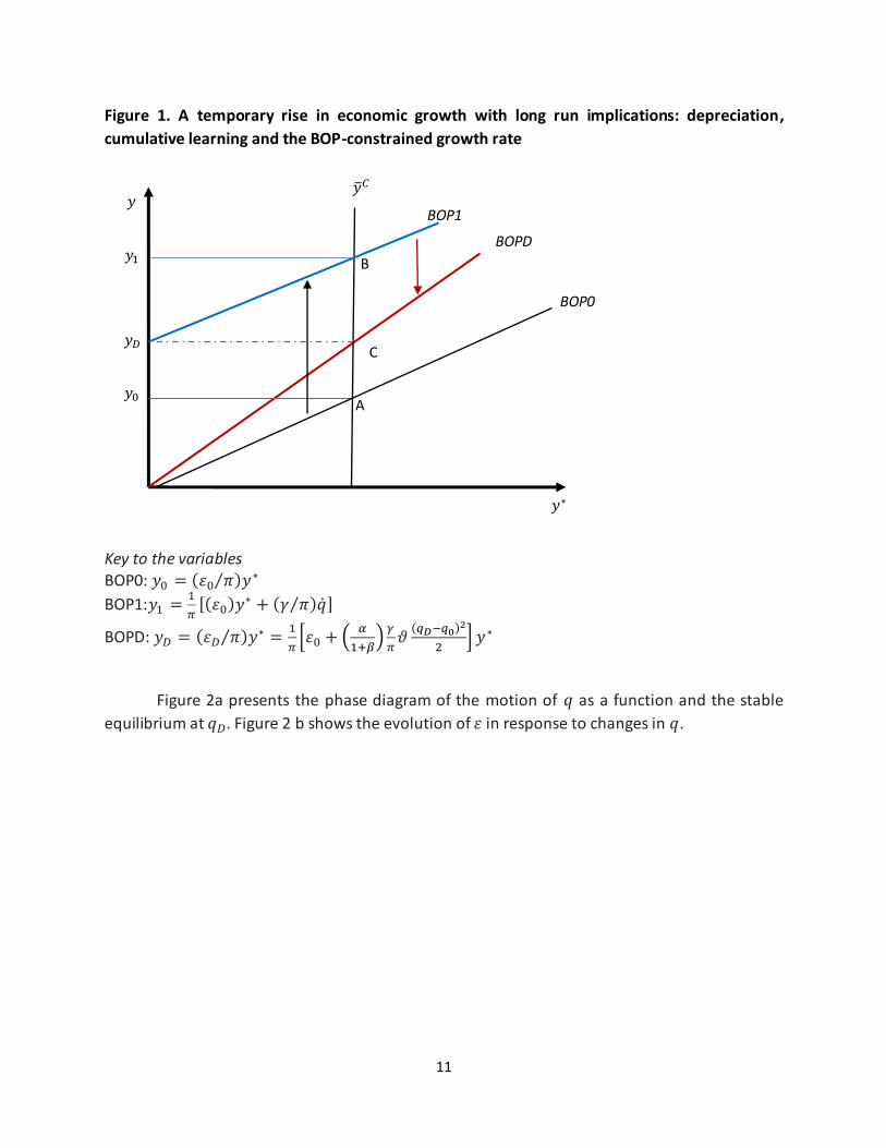
Figure 1 shows the adjustment process between two long-run equilibrium positions, always

assuming that Marshall-Lerner holds. Initially the economy is at point A, which represents the

BOP-constrained growth rate in equilibrium (𝑦0 = (𝜀0 𝜋⁄ )𝑦∗) for a given income elasticity of

exports 𝜀0. The RER is on its initial equilibrium value 𝑞0. The rise in the real exchange rate (from

𝑞0 to 𝑞𝐷) allows the economy to grow at a higher rate while the RER is depreciating (the BOP0

curve shifts to BOP1). The new BOP-constrained growth rate is 𝑦1 =1

𝜋[(𝜀0)𝑦

∗ + 𝛾 �̇�] in point

B. It is easy to see that the difference between BOP0 and BOP1 is that the BOP-constrained

growth rate schedule no longer passes through the origin. The intercept of the B0P1 curve is

(𝛾 𝜋⁄ )�̇� > 0.

When the depreciation process ends, the growth-enhancing effect of depreciation would

have ceased. However, the economy does not come back to BOP0 but to BOPD (the red line,

new equilibrium in C). The reason is, as mentioned, that during the period of faster growth new

investments and learning by doing allowed the economy to raise its income elasticity of

exports. The new equilibrium features a higher RER, a higher income elasticity of exports

(𝜀𝐷 > 𝜀0), and a higher rate of growth in equilibrium (𝑦𝐷 = (𝜀𝐷 𝜋⁄ )𝑦∗ > 𝑦0 = (𝜀0 𝜋⁄ )𝑦∗).

11

Figure 1. A temporary rise in economic growth with long run implications: depreciation,

cumulative learning and the BOP-constrained growth rate

Key to the variables BOP0: 𝑦0 = (𝜀0 𝜋⁄ )𝑦∗

BOP1:𝑦1 =1

𝜋[(𝜀0)𝑦

∗ + (𝛾 𝜋⁄ )�̇�]

BOPD: 𝑦𝐷 = (𝜀𝐷 𝜋⁄ )𝑦∗ =1

𝜋[𝜀0 + (

𝛼

1+𝛽)

𝛾

𝜋𝜗

(𝑞𝐷−𝑞0)2

2] 𝑦∗

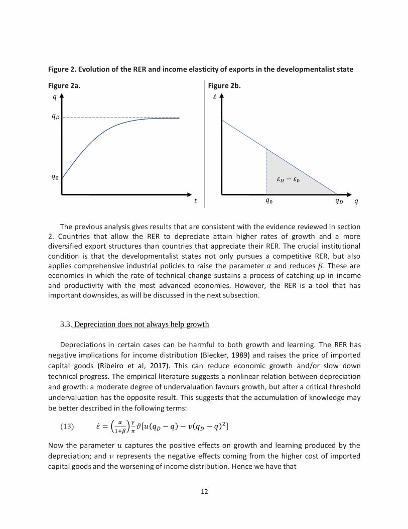
Figure 2a presents the phase diagram of the motion of 𝑞 as a function and the stable

equilibrium at 𝑞𝐷. Figure 2 b shows the evolution of 𝜀 in response to changes in 𝑞.

A

𝑦 𝐶

B

BOP1

BOP0

𝑦

𝑦∗

𝑦𝐷

𝑦0

𝑦1

C

BOPD

12

Figure 2. Evolution of the RER and income elasticity of exports in the developmentalist state

Figure 2a.

Figure 2b.

The previous analysis gives results that are consistent with the evidence reviewed in section 2. Countries that allow the RER to depreciate attain higher rates of growth and a more diversified export structures than countries that appreciate their RER. The crucial institutional condition is that the developmentalist states not only pursues a competitive RER, but also applies comprehensive industrial policies to raise the parameter 𝛼 and reduces 𝛽. These are economies in which the rate of technical change sustains a process of catching up in income and productivity with the most advanced economies. However, the RER is a tool that has important downsides, as will be discussed in the next subsection.

3.3. Depreciation does not always help growth

Depreciations in certain cases can be harmful to both growth and learning. The RER has

negative implications for income distribution (Blecker, 1989) and raises the price of imported

capital goods (Ribeiro et al, 2017). This can reduce economic growth and/or slow down

technical progress. The empirical literature suggests a nonlinear relation between depreciation

and growth: a moderate degree of undervaluation favours growth, but after a critical threshold

undervaluation has the opposite result. This suggests that the accumulation of knowledge may

be better described in the following terms:

(13) 𝜀̇ = (𝛼

1+𝛽)

𝛾

𝜋𝜗[𝑢(𝑞𝐷 − 𝑞) − 𝑣(𝑞𝐷 − 𝑞)2]

Now the parameter 𝑢 captures the positive effects on growth and learning produced by the

depreciation; and 𝑣 represents the negative effects coming from the higher cost of imported

capital goods and the worsening of income distribution. Hence we have that

𝑡

𝑞

𝑞

𝜀 ̇

𝑞0

𝑞𝐷

𝜀𝐷 − 𝜀0

𝑞0 𝑞𝐷

13

∫ 𝜀̇𝑞𝐷

𝑞0𝑑𝑞 = 𝜀𝐷 = 𝜀0 + (

𝛼

1+𝛽)

𝛾

𝜋𝜗∫ [𝑢(𝑞

𝐷− 𝑞) − 𝑣(𝑞

𝐷− 𝑞)

2]𝑑𝑞

𝑞𝐷

𝑞0 . That will results in:

(14) 𝜀𝐷 = 𝜀0 + (𝛼

1+𝛽)

𝛾

𝜋𝜗 [𝑢

(𝑞𝐷−𝑞0)2

2− 𝑣

(𝑞𝐷−𝑞0)3

3]

Equation (13) no longer implies that a higher 𝑞𝐷 necessarily leads to a higher 𝜀𝐷. This will

happen under the additional condition (besides industrial policy) that the difference between

the initial RER and the target RER is not too high. Specifically, for having a positive impact on

the income elasticity of exports, the distance between the two RERs must satisfy the following

inequality: 𝑞𝐷 − 𝑞0 < 3𝑢 2𝑣⁄ . In economies whose production is destined mostly to the

domestic market and which are highly dependent on imported capital goods, it is likely that 𝑣 is

high and 𝑢 is low. Hence, it is less likely that depreciation would help a process of capital and

knowledge accumulation. In those cases (high 𝑣 and low 𝑢), the RER is a rather inefficient

instrument for economic development.

4. Conflicting claims and the RER

In the previous section it was assumed that the developmentalist state has an unchallenged

grip on the RER. This is a good approximation to the case of a few cases in Asia. However, in

many developing economies there is resistance to depreciation. A higher RER means a lower

wage share in GDP. Depreciation has redistributive consequences that elicit a response from

workers’ unions. In some Latin American countries (such as Argentina and Uruguay) there are

strong labour unions that negotiate with the firms in a unified and structured way. This makes

unviable for governments or firms to unilaterally set the RER they prefer based solely on the

quest for international competitiveness. The following discussion is based on the analysis of

RER dynamics when actors’ preferences over the RER are heterogeneous, as suggested in Lima

and Porcile (2013).

4.1.Basic equations

We consider now the case in which workers consume imported goods. The cost of the workers’ consumption basket is 𝑃𝑊 = 𝑃𝜏(𝑃∗𝐸)1−𝜏 where 𝜏 is the share of domestic goods. The real wage in this economy is 𝜔 = 𝑊 𝑃𝜏(𝑃∗𝐸)1−𝜏⁄ . Since 𝑊 = 𝑃/𝑧𝑎 and 𝑞 = 𝑙𝑛(𝑃∗𝐸 𝑃⁄ ), then 𝜔 = 1 𝑧𝑎(𝑒𝑞)1−𝜏⁄ . As 𝑎 = 𝐿/𝑌, real workers’ consumption in GDP is:

(15) (𝜔𝐿) 𝑌⁄ = 1 𝑧(𝑒𝑞)1−𝜏⁄ .

It can be seen that there is a negative association between the real exchange rate and the

workers’ consumption share in GDP. If workers are organized, they will react to a real

14

depreciation. Workers will demand higher nominal wages when the RER is high so as to sustain

or increase real consumption. Formally, the increase in nominal wages will have two parts: a

term that captures the increase in labour productivity (�̂�); b) a term to correct the impact of the

RER on the cost of the labor consumption basket:

(16) �̂� = �̂� + 𝜍 [𝑙𝑛 (1

𝑧(𝑒𝑞𝑤)1−𝜏)− 𝑙𝑛(

1

𝑧(𝑒𝑞)1−𝜏)]

In equation (63) 𝑞𝑊 is the RER aimed at by the workers and 𝜍 the velocity the economy

moves to equilibrium in the labour market. This can be expressed as:

(17) �̂� − �̂� = ℎ(𝑞 − 𝑞𝑊), where ℎ ≡ 𝜍(1 − 𝜏)

We will keep the assumption that wages in the centre grow at the same rate as productivity

in the centre.

Workers are not the only actors in the game. The government uses the exchange rate policy

to sustain competitiveness and avoid an external crisis. Frequently, governments are more

reactive to the capitalists’ demands than to workers’ demands. If capitalists’ actors demand a

higher profit share in GDP and a higher RER to export and invest, their representatives in

government and parliament will make pressure in this direction. Consider the case discussed in

Lima and Porcile (2013) in which both workers and the government have different preferences

in terms of the RER. The government raises the rate of nominal devaluation if it sees that the

RER falls below the RER it considers necessary to sustain international competitiveness.

Formally:

(18) �̂� = 𝑗(𝑞𝐺 − 𝑞)

Recall that the rate of change of the RER is �̇� = �̂� + (𝑧 ∗̂ − �̂�) + (𝑎∗̂ − �̂�) + (𝑊 ∗̂ − �̂�). If

the mark-up is constant in centre and periphery and assuming (𝑊 ∗̂ = 𝑎∗̂), this expression

becomes �̇� = �̂� − �̂� + �̂� = �̂� − ℎ(𝑞 − 𝑞𝑊) (per equation 17)18. Using this result in (18), the

rate of change of the RER will be given by:

(19) �̇� = 𝑗(𝑞𝐺 − 𝑞) − ℎ(𝑞 − 𝑞𝑊)

We will normalize ℎ + 𝑗 = 1. Then the differential equation (19) produces a stable equilibrium

𝑞𝐸 when:

(20) 𝑞𝐸 = 𝑗𝑞𝐺 + (1− 𝑗)𝑞𝑊

Note that neither workers nor the government will ever be contented with the

equilibrium value of the RER (unless in the very special case in which 𝑞𝐺 = 𝑞𝑊, in which there

18 Since 𝑃 = 𝑊𝑧/𝑎, then the inflation rate (with a constant 𝑧) is �̂� = �̂� − �̂�. It is

straightforward that �̇� = 𝑃∗̂ + �̂� − �̂� and with 𝑃∗̂ = 0, then �̇� = −�̂� + �̂�, i.e. the rate of

change of the RER equals the negative of the inflation rate.

15

are no conflicting claims on income shares at all). 𝐸 and 𝑊 grows at the same rate (�̂� = �̂� − �̂�)

keeping the RER constant on the equilibrium value defined in equation (20). Since 𝑞𝑊 < 𝑞𝐺, the

higher the bargaining power of workers ℎ, the lower the RER in equilibrium; the higher the

concern of the government with competitiveness (𝑗)—and the efforts it makes for sustaining

it—the higher will be the RER. Indeed, it is easy to see that the authoritarian developmentalist

state is a special case of equation (19), in which 𝑗 = 1, becoming similar to equation (9).

4.2.The learning path

Now the BOP-constrained rate of growth in equilibrium in the medium run will be:

(21) 𝑦 =𝜀

𝜋𝑦∗ +

𝛾

𝜋 [𝑗(𝑞𝐺 − 𝑞) − (1 − 𝑗)(𝑞 − 𝑞𝑊)]

As in the previous section, the rate of learning and the transformation of the production

structure depend on the accumulated rate of growth over the initial equilibrium growth rate:

(22) 𝜀̇ = (𝛼

1+𝛽)

𝛾

𝜋�̇�

Using (19) in (22) gives:

(23) 𝜀̇ = (𝛼

1+𝛽)

𝛾

𝜋[𝑗(𝑞𝐺 − 𝑞) − (1 − 𝑗)(𝑞 − 𝑞𝑊)]

Integrating both sides of the equation between with respect to 𝑞 allows for finding the new

value of the income elasticity of exports when 𝑞 = 𝑞𝐸 :

∫ 𝜀̇𝑑𝑞𝑞𝐸

𝑞0

= (𝛼

1 + 𝛽) (

𝛾

𝜋) [

𝑞𝐸2

2+ (𝑗 − 1)𝑞𝑊𝑞

𝐸− 𝑗𝑞𝐺𝑞

𝐸−

𝑞02

2− (𝑗 − 1)𝑞𝑊𝑞

0+ 𝑗𝑞𝐺𝑞

0]

If we make 𝑗 = 1 and 𝑞𝐺 = 𝑞𝐷, equation (24) gives the same result as equation (12).

Some interesting points emerge from equation (24). First, if there is no industrial policy, the

higher the value of the RER in equilibrium, the higher the new income elasticity of exports.

There is a trade-off between the wage share and the BOP-constrained growth rate because

there is a trade-off between the wage share and the degree of diversification attained by the

economy when the RER is in equilibrium. Given 𝛼 and 𝛽, the road to diversification implies a fall

in the wage share (even though real wages may be increasing as the economy grows at a higher

rate in equilibrium).

Second, although the model does not capture the dynamics of wages and inflation behind

the stable RER, these dynamics may affect investment and learning. If the equality �̂� = �̂� is

satisfied at very high levels of wages increases and rates of nominal devaluations of the

exchange rate, inflation will be rampant, the intensity of conflict more acute and investment

16

will necessarily fall. Uncertainty and instability hamper technological change and the

transformation of the production structure.

Last but not least, an increase in 𝛼 and a fall in 𝛽 allows for a higher wage share for a given

long-run BOP-constrained rate of growth19. Industrial policy allows minor depreciations to

become an effective mechanism for diversifying the export structure. This explains why

industrial policy is important for sustaining growth without compromising, or even improving,

income distribution.

Industrial policy is central to mollify the distributive conflict in a democratic society in which

workers, capitalists and government have heterogeneous preferences over the RER. In the Latin

American countries, industrial policies had been highly ineffective (or inexistent), which made it

more difficult for them to arbitrate the contradiction between price competitiveness

(represented by the RER) and income distribution (represented by the wage share). There was

no rapid diffusion of technology (which would shift outward the external constraint on growth

and employment) to mollify the intensity of the distributive conflict. On the other hand, in

advanced democracies (such as those in Northern Europe, and especially in the Nordic

countries), highly institutionalized negotiations over wage shares and prices are combined with

a large set of incentives to innovation and diffusion of technology. This combination keeps

international competitiveness (based on technological learning) and equality moving hand in

hand20.

5. Financialization and the neoliberal coalition: slow growth and instability

The third scenario assumes that the game is between a state whose sole objective is to

control inflation and an international capital market that arbitrates between assets

denominated in domestic and foreign currencies. This is an economy with a fully open capital

account in which the government allows the RER to fluctuate as a function of short-term capital

flows and seeks to control inflation using a Taylor rule for the interest rate. We call this a

financialization scenario because the RER will depend on changes in the international financial

markets and the government commitment to fight inflation.

19 The wage share does not depend directly on 𝛼 and 𝛽, as 𝜔 = 1 𝑧𝑎(𝑒𝑞)1−𝜏⁄ . However, the trade off occurs in the

diversification equation (𝜀): 𝜀̇ = (𝛼

1+𝛽)

𝛾

𝜋[𝑗(𝑞𝐺 − 𝑞)− (1 − 𝑗)(𝑞 − 𝑞𝑊)]. A reduction in 𝑗 (and rise in 1 − 𝑗) can

only maintain a fixed 𝜀̇ with increases in 𝛼 and reduction in 𝛽. That would result in the same growth rate (𝑦).

20 Aa put by Andersen et al (2015): “In a sense it can be argued that competitiveness was enhanced by collective

bargaining based on the relatively pragmatic positions of dominant trade unions and employers’ associations. It is not that conflicts and power struggles were absent, rather there (…) a basic willingness to try to develop the

collective bargaining systems.” p.139.

17

5.1.Basic equations

Foreign capital will be attracted by the difference in the real interest rates at home and abroad. If real domestic interest rates are higher than the foreign interest rates, the domestic currency will be appreciated by capital inflows, as expressed in the following equation (where

𝑟𝑓is the international real interest rate, 𝜑 an adjustment parameter and 𝑟 the domestic real interest rate):

(24) �̇� = 𝜑(𝑟𝑓 − 𝑟)

The government of the peripheral country is mostly concerned with inflation and adopt

an inflation target 𝜃 which it pursues using monetary policy. From equations (17), nominal

wages will rise faster when the RER is higher than the RER aimed at by the workers. A rise in

nominal wages, for a given rate of growth of productivity and a fixed mark-up, raises the

inflation rate. The government will try to curb the surge in inflation by increasing the real

interest rate to reduce aggregate demand. The reaction curve of the policy-maker can be

expressed as a simple Taylor rule:

(25) �̇� = 𝜌0(�̂� − 𝜃) − 𝜌1𝑟 = 𝜌0[ℎ(𝑞 − 𝑞𝑊) − 𝜃] − 𝜌1𝑟 = −𝑔 + 𝜌𝑞 − 𝜌1𝑟

Where 𝑔 ≡ 𝜌𝑞𝑊 − 𝜃 and 𝜌 ≡ 𝜌0ℎ. The increase of the real interest rate will be a

positive function of the RER (which boosts inflation) and a negative function of the real interest

rate (which reduces aggregate demand). The system is stable, and the equilibrium values are:

(26) 𝑟𝐸 = 𝑟𝑓

(27) 𝑞𝐸 =𝑔+𝜌1𝑟

𝑓

𝜌

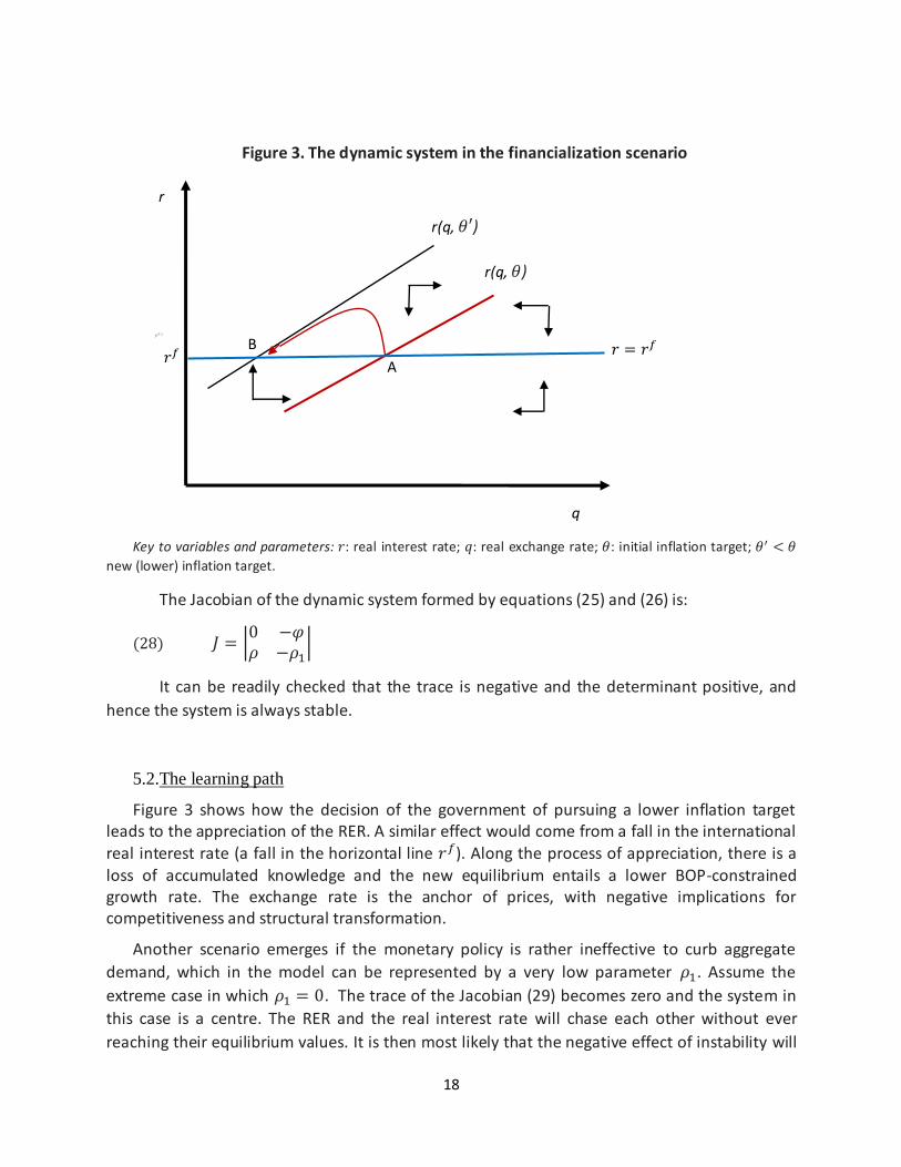
Figure 3 shows the phase diagram of the system of differential equations formed by

equations (27) and (28). Assume that the economy is initially at point A, and that the

government adopts a stricter target for the inflation rate (𝜃′ < 𝜃). The �̇� = 0 isocline shifts to

the left. To attain 𝜃′, the government increases the real interest rate, which leads to inflows of

foreign capital that appreciates the RER. Gradually, the appreciation of the RER helps control

inflation and the interest rate becomes less necessary to attain the new inflation target. The

adjustment process ends with the same real interest rate as before (which is the international

interest rate) and a lower real exchange rate in equilibrium.

18

Figure 3. The dynamic system in the financialization scenario

Key to variables and parameters: 𝑟: real interest rate; 𝑞: real exchange rate; 𝜃: initial inflation target; 𝜃′ < 𝜃

new (lower) inflation target.

The Jacobian of the dynamic system formed by equations (25) and (26) is:

(28) 𝐽 = |0 −𝜑𝜌 −𝜌1

|

It can be readily checked that the trace is negative and the determinant positive, and

hence the system is always stable.

5.2.The learning path

Figure 3 shows how the decision of the government of pursuing a lower inflation target leads to the appreciation of the RER. A similar effect would come from a fall in the international real interest rate (a fall in the horizontal line 𝑟𝑓). Along the process of appreciation, there is a loss of accumulated knowledge and the new equilibrium entails a lower BOP-constrained growth rate. The exchange rate is the anchor of prices, with negative implications for competitiveness and structural transformation.

Another scenario emerges if the monetary policy is rather ineffective to curb aggregate

demand, which in the model can be represented by a very low parameter 𝜌1. Assume the

extreme case in which 𝜌1 = 0. The trace of the Jacobian (29) becomes zero and the system in

this case is a centre. The RER and the real interest rate will chase each other without ever

reaching their equilibrium values. It is then most likely that the negative effect of instability will

A

B

r(q, 𝜃)

𝑟 = 𝑟𝑓 𝑟𝑓

r

q

r(q, 𝜃′)

19

overcome any potential positive effect of depreciation on growth. Such instability increases

with the radio of the circle defined by the orbit of the variables 𝑟 and 𝑞.

Given the initial position of the economy (the initial value of 𝑟 and 𝑞), the economy is

permanently moving in circles around the equilibrium point without never reaching it. What are

the implications for structural transformation of this kind of dynamics?

If fluctuations are small and predictable, they play no relevant role in decision making. If

these fluctuations are wide, even if they were predictable, there compromise investment.

Assume that investment increases when the BOP-constraint is eased (�̇� > 0) and decreases

when the BOP-constraint becomes more severe (�̇� < 0). In addition, assume that:

(29) 𝜀̇ = (𝛼

1+𝛽1)

𝛾

𝜋�̇�, if �̇� > 0

(30) 𝜀̇ = (𝛼

1+𝛽2)

𝛾

𝜋�̇�, if �̇� < 0

Assume now 𝛽1 > 𝛽221. This assumption implies that the inertial forces are stronger when

the economy is recovering than when the economy is losing capabilities. The rationale for this

assumption is that building capabilities is a more difficult process (especially in a world in which

technical change is extremely fast) than the loss of capabilities. It is necessary to run to stay in

the same place (the “Red Queen Effect”). Institutions are not easily reconstructed; the skills lost

in one period will not be available in the next; firms, networks and externalities will no longer

be at hand. This is a hysteresis scenario which not only hinders structural transformation, but

also implies regressive structural change after each appreciation / depreciation cycle of the

RER. The economy cannot take the same path back to its previous equilibrium after the

alteration of its economic structure. The description of an economy with a downward trend in

competitiveness may not be realistic for a very long run, but it does represent protracted

growth phases in developing economies, especially after a severe external crisis.

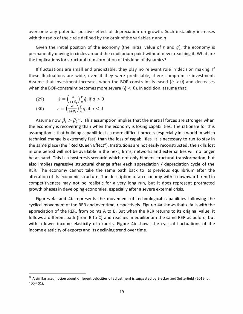
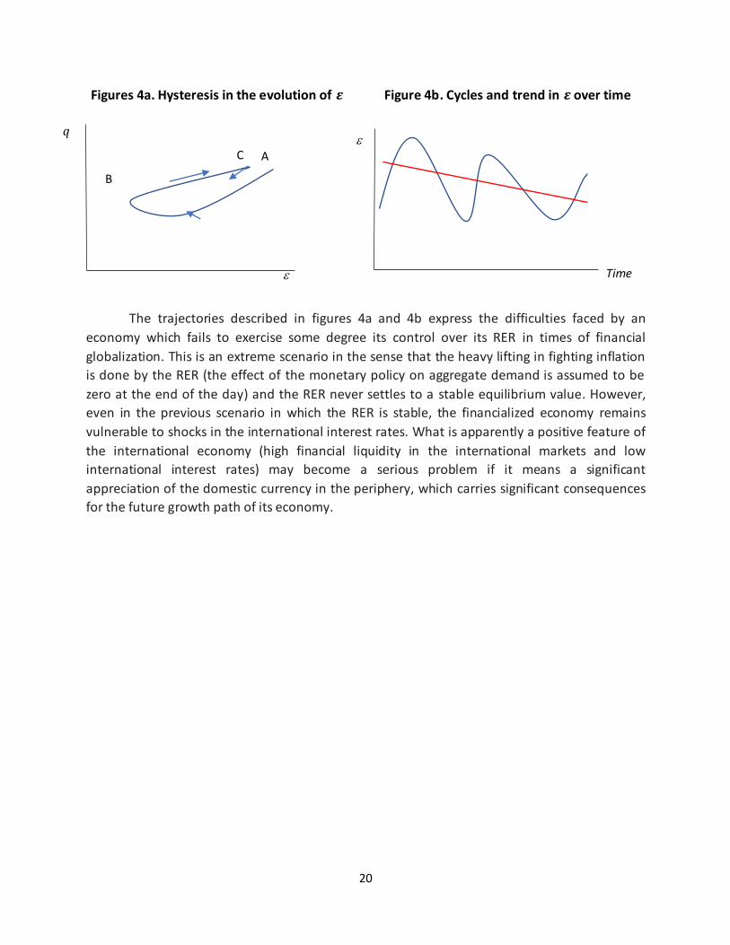
Figures 4a and 4b represents the movement of technological capabilities following the

cyclical movement of the RER and over time, respectively. Figurer 4a shows that 𝜀 falls with the

appreciation of the RER, from points A to B. But when the RER returns to its original value, it

follows a different path (from B to C) and reaches in equilibrium the same RER as before, but

with a lower income elasticity of exports. Figure 4b shows the cyclical fluctuations of the

income elasticity of exports and its declining trend over time.

21 A similar assumption about different velocities of adjustment is suggested by Blecker and Setterfield (2019, p.

400-401).

20

Figures 4a. Hysteresis in the evolution of 𝜺 Figure 4b. Cycles and trend in 𝜺 over time

The trajectories described in figures 4a and 4b express the difficulties faced by an

economy which fails to exercise some degree its control over its RER in times of financial

globalization. This is an extreme scenario in the sense that the heavy lifting in fighting inflation

is done by the RER (the effect of the monetary policy on aggregate demand is assumed to be

zero at the end of the day) and the RER never settles to a stable equilibrium value. However,

even in the previous scenario in which the RER is stable, the financialized economy remains

vulnerable to shocks in the international interest rates. What is apparently a positive feature of

the international economy (high financial liquidity in the international markets and low

international interest rates) may become a serious problem if it means a significant

appreciation of the domestic currency in the periphery, which carries significant consequences

for the future growth path of its economy.

𝑞

Time

A

B

C

21

6. Concluding remarks

The empirical literature on RER and growth reports conflicting results, which are highly

sensitive to the inclusion or not of a technological variable in the econometric exercises. We

suggest a BOP-constrained growth model which can explain these mixed results as a function of

the interplay between two kinds of policies, the exchange rate policy and the industrial policy.

Such policies shape the institutional framework in which technological learning takes place and

the RER evolves. We identify three institutional frameworks that express different political

regimes and political dynamics: the developmentalist state, conflicting claims over

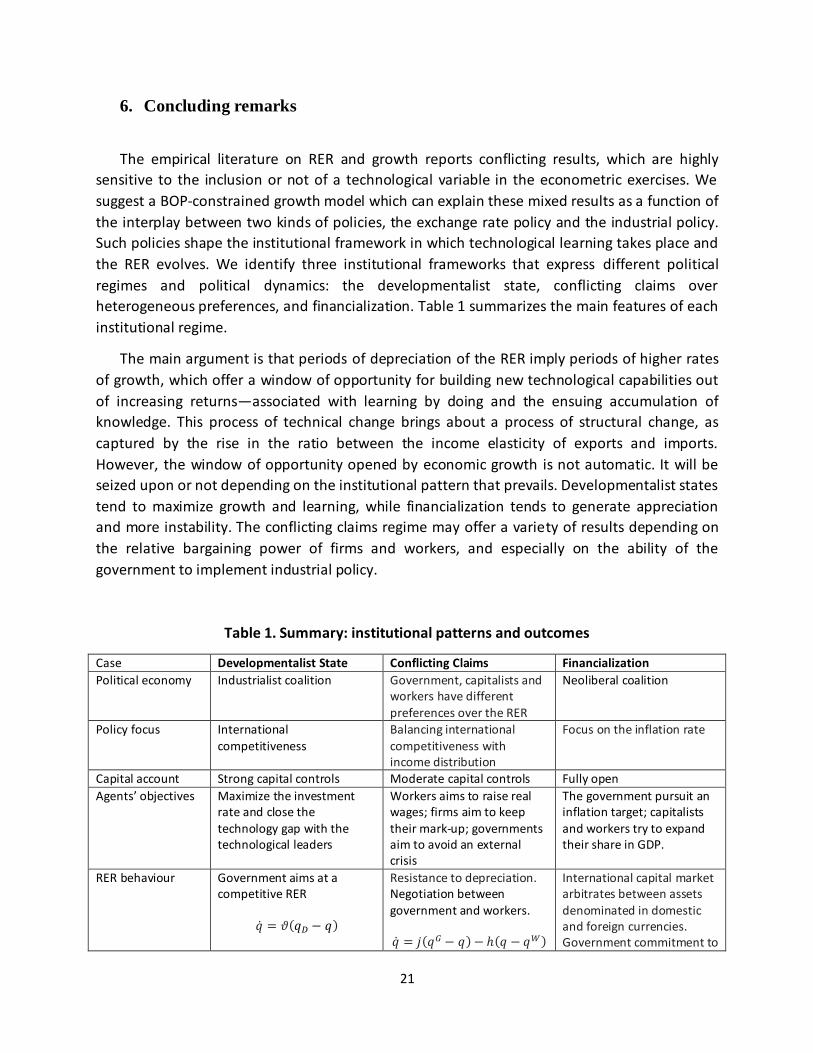
heterogeneous preferences, and financialization. Table 1 summarizes the main features of each

institutional regime.

The main argument is that periods of depreciation of the RER imply periods of higher rates

of growth, which offer a window of opportunity for building new technological capabilities out

of increasing returns—associated with learning by doing and the ensuing accumulation of

knowledge. This process of technical change brings about a process of structural change, as

captured by the rise in the ratio between the income elasticity of exports and imports.

However, the window of opportunity opened by economic growth is not automatic. It will be

seized upon or not depending on the institutional pattern that prevails. Developmentalist states

tend to maximize growth and learning, while financialization tends to generate appreciation

and more instability. The conflicting claims regime may offer a variety of results depending on

the relative bargaining power of firms and workers, and especially on the ability of the

government to implement industrial policy.

Table 1. Summary: institutional patterns and outcomes

Case Developmentalist State Conflicting Claims Financialization

Political economy Industrialist coalition Government, capitalists and workers have different preferences over the RER

Neoliberal coalition

Policy focus

International

competitiveness

Balancing international

competitiveness with income distribution

Focus on the inflation rate

Capital account Strong capital controls Moderate capital controls Fully open

Agents’ objectives Maximize the investment rate and close the technology gap with the technological leaders

Workers aims to raise real wages; firms aim to keep their mark-up; governments aim to avoid an external crisis

The government pursuit an inflation target; capitalists and workers try to expand their share in GDP.

RER behaviour Government aims at a competitive RER

�̇� = 𝜗(𝑞𝐷 − 𝑞)

Resistance to depreciation. Negotiation between

government and workers. �̇� = 𝑗(𝑞𝐺 − 𝑞)− ℎ(𝑞 − 𝑞𝑊)

International capital market arbitrates between assets

denominated in domestic and foreign currencies. Government commitment to

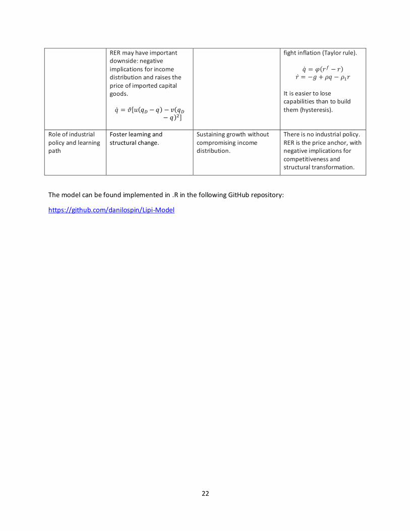
22

RER may have important downside: negative

implications for income distribution and raises the price of imported capital goods. �̇� = 𝜗[𝑢(𝑞𝐷 − 𝑞) − 𝑣(𝑞𝐷

− 𝑞)2]

fight inflation (Taylor rule).

�̇� = 𝜑(𝑟𝑓 − 𝑟) �̇� = −𝑔 + 𝜌𝑞 − 𝜌1𝑟

It is easier to lose capabilities than to build them (hysteresis).

Role of industrial

policy and learning path

Foster learning and

structural change.

Sustaining growth without

compromising income distribution.

There is no industrial policy.

RER is the price anchor, with negative implications for competitiveness and structural transformation.

The model can be found implemented in .R in the following GitHub repository:

https://github.com/danilospin/Lipi-Model

23

Bibliography

Agosin, M. R., Alvarez, R., & Bravo‐Ortega, C. (2012). Determinants of Export Diversification Around the

World: 1962–2000. The World Economy, 35, 295–315.

Andersen, S. K., Ibsen, C. L., Alsos, K., Neergaard, K., & Sauramo, P. (2015). Wage bargaining under the

new European Economic Governance: Alternative strategies for inclusive growth. ETUI.

Araujo, R. A. (2013). Cumulative causation in a structural economic dynamic approach to economic

growth and uneven development. Structural Change and Economic Dynamics, 24, 130–140.

Araujo, R. A., & Lima, G. T. (2007). A structural economic dynamics approach to balance-of-payments-

constrained growth. Cambridge Journal of Economics, 31, 755–774.

Berg, A., Ostry, J., & Zettelmeyer, J. (2012). What makes growth sustained? Journal of Development

Economics, 98, 149–166.

Blecker, R. A. (1989). International competition, income distribution and economic growth. Cambridge

Journal of Economics, 13, 395–412.

Blecker, R. A., & Setterfield, M. (2019). Heterodox macroeconomics: Models of demand, distribution and

growth.

Boggio, L., & Barbieri, L. (2017). International competitiveness in post-Keynesian growth theory:

Controversies and empirical evidence. Cambridge Journal of Economics, 41, 25–47.

Caglayan, M., & Demir, F. (2019). Exchange rate movements, export sophistication and direction of

trade: The development channel and North–South trade flows. Cambridge Journal of Economics,

43, 1623–1652.

Cimoli, M., Fleitas, S., & Porcile, G. (2013). Technological intensity of the export structure and the real

exchange rate. Economics of Innovation and New Technology , 22, 353–372.

Cimoli, M., & Porcile, G. (2014). Technology, structural change and BOP-constrained growth: A

structuralist toolbox. Cambridge Journal of Economics, 38, 215–237.

Cimoli, M., Porcile, G., & Rovira, S. (2010). Structural change and the BOP-constraint: Why did Latin

America fail to converge? Cambridge Journal of Economics, 34, 389–411.

Diaz-Alejandro, C. F. (1986). The Early 1980s in Latin America: The 1930s One More Time? In Theory and

Reality in Development (pp. 154–164). Palgrave Macmillan, London.

Dutt, A. K. (1992). A Kaldorian Model of Growth and Development Revisited: A Comment on Thirlwall.

Oxford Economic Papers, 44, 156–168.

24

Dvoskin, A., Feldman, G. D., & Ianni, G. (2020). New-structuralist exchange-rate policy and the pattern of

specialization in Latin American countries. Metroeconomica, 71, 22–48.

Eichengreen, B. J. (2007). The European economy since 1945: Coordinated capitalism and beyond.

Princeton: Princeton University Press.

Frenkel, R., & Ros, J. (2006). Unemployment and the real exchange rate in Latin America. World

Development, 34, 631–646.

Freund, C., & Pierola, M. D. (2012). Export surges. Journal of Development Economics, 97, 387–395.

Gabriel, L. F., Ribeiro, L. C. D. S., Jr, F. G. J., & Oreiro, J. L. (2020). Manufacturing, economic growth, and

real exchange rate: Empirical evidence in panel data and input-output multipliers. PSL Quarterly

Review, 73, 51–75.

Ibarra, C. A., & Blecker, R. A. (2016). Structural change, the real exchange rate and the balance of

payments in Mexico, 1960–2012. Cambridge Journal of Economics, 40, 507–539.

Kaldor, N. (1978). The Effect of Devaluation on Trade in Manufacturers. Future Essays in Applied

Economics, 99–116.

Krugman, P., & Taylor, L. (1978). Contractionary effects of devaluation. Journal of International

Economics, 8, 445–456.

Lee, K. (2013). Schumpeterian analysis of economic catch-up: Knowledge, path-creation, and the middle-

income trap.

Lima, G. T., & Porcile, G. (2013). Economic growth and income distribution with heterogeneous

preferences on the real exchange rate. Journal of Post Keynesian Economics, 35, 651–674.

Lundvall, B.-Å. (2016). The learning economy and the economics of hope. Retrieved from http://0-

www.cambridge.org.pugwash.lib.warwick.ac.uk/core/product/identifier/9781783085972/type/

BOOK

Marconi, N., Magacho, G., Machado, J. G. R., Leão, R. (2020). Profit margins, exchange rates and

structural change: Empirical evidences for the period 1996-2017. Brazilian Journal of Political

Economy, 40, 285–309.

Marconi, N., Reis, C. F. de B., & Araújo, E. C. de. (2016). Manufacturing and economic development: The

actuality of Kaldor’s first and second laws. Structural Change and Economic Dynamics, 37, 75–

89.

McMillan, M., Rodrik, D., & Verduzco-Gallo, Í. (2014). Globalization, Structural Change, and Productivity

Growth, with an Update on Africa. World Development, Complete, 11–32.

25

Medeiros, C. A. de. (2020). A Structuralist and Institutionalist developmental assessment of and reaction

to New Developmentalism. Review of Keynesian Economics, 8, 147–167.

Missio, F. J., Jayme, F. G., Britto, G., & Luis Oreiro, J. (2015). Real Exchange Rate and Economic Growth:

New Empirical Evidence. Metroeconomica, 66, 686–714.

Nassif, A., Feijó, C., & Araújo, E. (2015). Structural change and economic development: Is Brazil catching

up or falling behind? Cambridge Journal of Economics, 39, 1307–1332.

Nelson, R. R., & Sampat, B. N. (2001). Making sense of institutions as a factor shaping economic

performance. Journal of Economic Behavior & Organization, 44, 31–54.

Nucci, F., & Pozzolo, A. F. (2001). Investment and the exchange rate: An analysis with firm-level panel

data. European Economic Review, 45, 259–283.

Porcile, G., & Spinola, D. S. (2018). Natural, Effective and BOP-Constrained Rates of Growth: Adjustment

Mechanisms and Closure Equations. PSL Quarterly Review, 71, 139–160.

Rapetti, M., Skott, P., & Razmi, A. (2012). The real exchange rate and economic growth: Are developing

countries different? International Review of Applied Economics, 26, 735–753.

Ribeiro, R., McCombie, J., & Lima, G. T. (2016). Exchange Rate, Income Distribution and Technical

Change in a Balance-of-Payments Constrained Growth Model. Review of Political Economy, 28,

545–565.

Ribeiro, R., McCombie, J., & Lima, G. T. (2017). A reconciliation proposal of demand-driven growth

models in open economies. Journal of Economic Studies, 44, 226–244.

Ribeiro, R., McCombie, J., & Lima, G. T. (2019). Does real exchange rate undervaluation really promote

economic growth? Structural Change and Economic Dynamics, 52, 408-417.

Rodrik, D. (2008). The Real Exchange Rate and Economic Growth. Brookings Papers on Economic Activity,

2008, 365–412.

Setterfield, M. (2002). The Economics of Demand-Led Growth [Books]. Edward Elgar Publishing.

Setterfield, M. (2011). The remarkable durability of Thirlwall’s Law. PSL Quarterly Review, 64, 393–427.

Setterfield, M., & Cornwall, J. (2002). A Neo-Kaldorian Perspective on the Rise and Decline of the Golden

Age. In Chapters. Edward Elgar Publishing.

Storm, S., & Naastepad, C. W. M. (2015). Crisis and recovery in the German economy: The real lessons.

Structural Change and Economic Dynamics, 32, 11–24.

Taylor, L. (2004). Reconstructing macroeconomics: Structuralist proposals and critiques of the

mainstream. Cambridge, Mass.: Harvard University Press.

26

Thirlwall, A. P. (1979). The balance of payments constraint as an explanation of the international growth

rate differences. PSL Quarterly Review, 32.

Verdoorn, P. J. (2002). Factors that Determine the Growth of Labour Productivity. In J. McCombie, M.

Pugno, & B. Soro (Eds.), Productivity Growth and Economic Performance: Essays on Verdoorn’s

Law (pp. 28–36). London: Palgrave Macmillan UK.

Vieira, F. V., Holland, M., Silva, C. G. da, & Bottecchia, L. C. (2013). Growth and exchange rate volatility: A

panel data analysis. Applied Economics, 45, 3733–3741.

Vieira, Flavio Vilela, & MacDonald, R. (2016). Exchange rate volatility and exports: A panel data analysis.

Journal of Economic Studies, 43, 203–221.