Patterns of Coherent Decadal and Interdecadal Climate Signals in the Pacific Basin duringthe 20th Century

(AGU/GRL“Highlights”, May 15 2001)(Received December, 18, 2000; revised February, 13, 2001; accepted February, 26, 2001.)

by

Yves M. Tourre1, Balaji Rajagopalan1, Yochanan Kushnir1, Mathew Barlow2

1 Lamont Doherty Earth Observatory (LDEO) and 2International Research Institute for ClimatePrediction (IRI) of Columbia University, Palisades, NY.

Warren B. White3

3Scripps Institution of Oceanography (SIO) of University of California San Diego, La Jolla, CA.

Abstract. Two distinct low-frequency fluctuations are suggested from a joint frequency domain analysisof the Pacific Ocean (30°S-60°N) sea surface temperature (SST) and sea level pressure (SLP). The lowestfrequency signal reveals a spatially coherent interdecadal evolution. In-phase SST and SLP anomalies arefound along the subarctic frontal zone (SAFZ). It is symmetric about the equator, with tropical SSTanomalies peaking near 15° latitudes in the eastern Pacific. The other low-frequency signal reveals aspatially coherent decadal evolution. It is primarily a low-latitude phenomenon. Tropical SST anomaliespeak in the central equatorial ocean with evidence of atmospheric teleconnections. These interdecadal anddecadal signals join the ENSO and quasi-biennial signals in determining dominant patterns of PacificOcean natural climate variability. Relative phasing and location of the SST and SLP anomalies for thedecadal, ENSO, and the quasi-biennial signals, are similar to one another but significantly different fromthat of the interdecadal signal.

Introduction

Global low-frequency climate variability hasbeen identified (Mann and Park, 1996). In the PacificOcean and neighboring regions, patterns of low-frequency fluctuations within the climate andecological systems have been referred to as the“Pacific (inter) Decadal Oscillation or PDO" (Mantuaet al., 1997), the “Inter-decadal Pacific Oscillation orIPO (Power et al., 1999), the Pacific "Decadal andInterdecadal Climatic Event or DICE" (Nakamuraand Yamagata, 1996) or as the “Bi-DecadalOscillation or BDO” (Cook et al., 1997). Evidencealso exists that low-frequency climate fluctuationsmodulate El Niño intensity (Torrence and Webster,1999).

In this paper, joint relationships betweenSST and SLP anomalies for the Pacific Ocean are

extracted based on spatial coherence at respectivefrequency bands, and show a significant distinctionbetween decadal and interdecadal fluctuations.Relationships between these distinct low-frequencysignals and the Pacific ENSO may assist inimproving climate prediction (Gershunov andBarnett, 1998). Recent modeling results (e.g.,Kleeman et al., 1999), should contribute to theevaluation of physical mechanisms associated withthese climate fluctuations. By incorporating this newinformation into decision-making schemes (e.g.,Meinke et al., 2000a), it is hoped global impacts ofrecurring drought/flood can be mitigated (Balmasedaet al.,1995).

Data and Results

A Multi-Taper-Method/Singular ValueDecomposition (MTM/SVD) technique with threetapers (Mann and Park, 1999) is applied to 92 years(1900-1991) of SST and SLP gridded datasets

(Kaplan et al., 1998). The three tapers allow forreasonable frequency resolution and providesufficient degrees of freedom for a signal/noisecomposition. The joint local fractional variance

2

(LFV) spectrum represents a fraction of variance in aparticular narrow frequency band associated withslow temporal modulation. Stability of the analysiswas tested by comparing results based upon the fullperiod (1900-1991) and the 1950-1990 period.Impacts of systematic biases in data collection weretested by introducing artificial data gaps. Astatistically significant separation of two low-frequency bands that represent independentinformation about spatially correlated oscillatorysignals -- the interdecadal and the decadal/quasi-decadal signals -- is obtained. The spatial evolutionof the signals is presented hereafter.

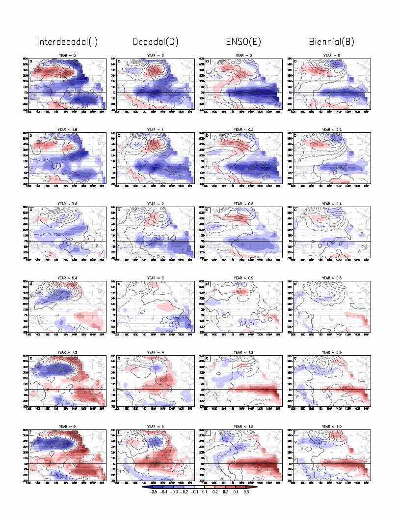
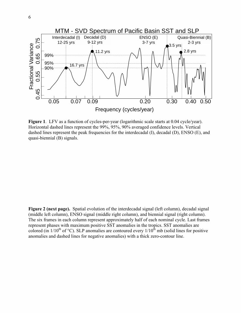
In Fig. 1, the LFV spectrum of the first jointSST-SLP singular values is displayed. Thestandardized anomalies are latitudinally weighted.The significance of peaks and frequency-bands in theLFV spectrum are determined through bootstraptime-resampling estimates (Efron, 1990) of the nulldistribution of a spatio-temporal “colored noise”. Thepotential bias from serial correlation was minimizedby permuting 1000 times, at random and separately,for the 92-yr annual sequences for each of the 12months of the year (Mann and Park, 1996). Theinterdecadal band peaks within the 16 to 17-yearperiods at the 90% confidence level (I in Figs. 1 and2). The decadal band peaks within the 10.8 to 11.9-year periods at the 99% confidence level (D in Figs. 1and 2). The ENSO band peaks at the 99% confidencelevel, within a range of 3 to 7-year periods (E in Figs.1 and 2). Within this ENSO band, several peaks areless well separated from the noise background andare probably associated with other complexfrequency-domain structures. The maximum LFV(~0.73) within the ENSO frequency-band peaks at a3.5-year period. The evolution of this peak ischaracteristic of that of other ENSO peaks (above99% confidence level) and so is reproduced in Figure2. The quasi-biennial band (2 to 3-yr periods, B inFigs. 1 and 2) contributes significantly to the LFVspectrum. From Fig.1 the joint SST-SLP spatialpatterns and their evolution of the lead 16.7-yearinterdecadal (I), lead 11.2-year decadal (D), leadcharacteristic 3.5-year ENSO (E), and lead 2.8-yearquasi-biennial (B) signals are reconstructed for one-half cycle. They are displayed in Figure 2 (leftcolumn for I, left middle column for D, right middlecolumn for E, and right column for B, respectively),from maximum tropical cooling to maximum tropicalwarming.

For the interdecadal signal (Fig. 2, leftcolumn), SST and SLP anomalies evolution is verysimilar to that featured in Tourre at al. (1999).Midlatitude SLP anomalies are found to develop in

the North Central Pacific around 45°N (Fig. 2, Ic).Significant midlatitude SST anomalies occur between25°N-45°N and 170°E-160°W and amplify along thesubarctic frontal zone (SAFZ) while SLP anomaliesof the same polarity keep developing eastward andpoleward (Fig.2, Id to If) indicating possible couplingand feedback mechanisms between the ocean andatmosphere there (Peng and Witaker, 1999). This isalso the time when SST anomalies (with oppositepolarity) develop rapidly along the North and SouthAmerican coastlines (Fig. 2, Ie and If). The offshoreSST anomalies in the eastern ocean are probablymaintained by anomalous oceanic vertical circulationassociated with co-varying SST and SLP anomaliesto the west, yielding along-shore wind anomalies.The portion of the SST anomaly pattern arising frompossible advection of SST anomalies extends slowlyequatorward following the Californian Current, theHumboldt Current, and the South Equatorial Currentor SEC (Fig. 2, Id to If). The maximum anomalies inthe North Pacific Ocean are not found south of 10°N,apparently due to the North Equatorial CounterCurrent. Conversely, the SST anomalies in the SouthPacific Ocean penetrate all the way to the equator inthe central and western Pacific Ocean. Thehemispheric symmetry displayed in Figure 2 (leftcolumn) emphasizes the role of the generalcirculation in the tropical South Pacific Oceanadvecting SST anomalies onto the equator via theSEC. During the tropical warm phase of theinterdecadal signal, maximum SST anomalies in theeastern ocean are found away from the equator near15°N and 15°S, and maximum SLP anomalies arefound at 45°N possibly modulating the intensity ofthe Aleutian Low. In the western ocean SSTanomalies occur on the equator between 160°E andthe dateline, where maximum salinity andtemperature gradients are usually found (Picaut et al.,1996). The tropical SLP fluctuations contribute toSouthern Oscillation variability (Fig. 2, Ie and If).When, in the midlatitudes, SST anomalies of a givenpolarity decrease slowly along the SAFZ (Fig. 2, Ia toIc) subduction from the outcrop region of the gyreoccurs at 10-15 m/year while anomalies of upper-ocean heat content extend slowly southwestwardwithin the subtropical gyre to reach the PhilippinesSeas 8-10 years later (Tourre et al., 1999).

For the decadal signal (Fig. 2, left middlecolumn), SST anomalies are found to amplify fromthe northeast tropical Pacific into the centralequatorial Pacific Ocean (Fig. 2, Dd to Df).Simultaneously SLP anomalies of opposite polarityamplify around 40°N, approximately within the samelongitudinal band between 120°W and 160°W. SST

3

anomalies of opposite polarity amplify in themidlatitudes around 40°N and between 140°W andthe dateline, probably due to maximum wind actionthere and resultant mean Ekman transport in nearsurface mixed layer of the ocean (Auad et al., 1998b).Subsequent evolution of tropical SST anomalies, isreminiscent of slow ENSO boundary waves andKelvin-Rossby wave dynamics (White et al., 1989)(Fig. 2, De and Df to Da and Db with opposite

polarity). The development of midlatitude SLPanomalies in the northeast Pacific Ocean, suggestsatmospheric teleconnections in response to SST-induced tropical convection, as on ENSO timescales(Graham, 1994). This mechanism is a good candidatefor maintaining the year-to-year persistence ofanomalous intensity of the Aleutian Low (Grahamand White, 1988).

Discussion and Conclusion

Low-frequency climate variability in thePacific Ocean consists at least of two spatiallycoherent signals in covarying SST and SLPanomalies: interdecadal and decadal signals, withdistinct spatial evolutions that invoke differentphysical processes to maintain their amplitudesagainst dissipation. Additional evidence is presentedhere for the interdecadal signal to be maintained inthe midlatitudes along the SAFZ through coupledocean-atmosphere dynamics (see also Auad et al.,1998b; White and Cayan, 1998; Barnett et al., 1999).The signal is then advected by the mean gyrecirculation (White and Cayan, 1998), where itcommunicates back to the midlatitudes, possibly ofboth hemispheres via atmospheric teleconnections.As such, the interdecadal signal requires meanadvection to provide for the necessary feedback andthe characteristic timescale of the phenomenon.Decadal, ENSO, and quasi-biennial signals requireRossby wave physics to provide the feedback and thecharacteristic timescales. The low-frequency decadaloscillation or PDO as previously defined in theliterature does not provide for the distinction betweenthe interdecadal and decadal Pacific signals. Analysisbased on spatial coherence of standing modesextracts two distinct spatial patterns of low-frequencyvariability in the North Pacific Basin (Barlow et al.,2000). The two spatial patterns are shown here to betwo distinct "snapshots" in the evolution of theinterdecadal signal (Fig. 2, d and f). Both spatialpatterns are associated with stationary atmosphericwave activity projected across North America andsignificant variations in drought and wet spells there.

The distinct separation between the two low-frequency signals is further clarified through closerexamination of the SLP evolution. With theinterdecadal signal, the development of SLP anomalyin the North Pacific occurs before the development oflocal SST anomalies of the same polarity (Fig. 2, Iband Ic). The North Pacific SLP anomalies switchpolarity and are already large by the time the switchoccurs in SST anomalies (Fig. 2, Id). With thedecadal signal, the extratropical SLP and SST

anomalies develop more or less together with samepolarity.

Differences in the evolution of SST-SLPanomalies associated with I, D, E and B, are seen inthe Tropics. The interdecadal tropical SST anomaliesreach maximum values away from the equator near15° latitudes (North and South), associated with theadvection of anomalies by mean currents in bothhemispheres. Tropical phasing of these interdecadalanomalies can modify the tropical ocean thermal andatmospheric pressure large scale patterns,contributing to the Southern Oscillation variability(Fig. 2, Ie and If) and possibly to the modulation ofthe intensity and evolution of El Niño (e.g., Kirtmanand Schopf, 1998). We show here how the decadalsignal evolves rapidly, from the central equatorialPacific, into an ENSO-like pattern. This suggests thatsubtropical Rossby wave dynamics may beresponsible for making the decadal signal evolve asan extended Pacific ENSO signal, providing thedelayed-negative feedback mechanism that gives thedecadal signal its characteristic time scale (e.g.,Jacobs et al., 1994). We also suggest that thesimilarity in the evolution of D, E, and B is sufficientto hypothesize that the three signals share the samebasic physics. The main similar feature is thedevelopment of large equatorial SST anomaly, withslightly lagged development of weaker extratropicalanomaly of opposite sign around 40°N and from thecentral Pacific toward the northwest Pacific (decadalto quasi-biennial respectively). The development andphasing of SLP relative to SST anomalies in themidlatitudes is also quite similar among the threesignals. In the tropics the three SLP signals contributeto Southern Oscillation variability with well-definedzero-line anomalies around the dateline (Fig. 2, Da,Ef and Bf). One of the difference among the threesignals is that E and B originate in the southeastPacific Ocean along the South American coastline,progressing westward along the equator. In contrast,D evolves from the central equatorial Pacific Oceanand expands eastward along the equator. But some

4

specific episodes have evolved differently (Tourreand White, 1995).Understanding the dynamics of low-frequencyfluctuations may yield considerable predictivecapabilities since low-frequency modes have beencorrelated with rainfall patterns in ENSO sensitiveregions across the Indo-Pacific basin (Allan, 2000).Research involving climate and climate applications

scientists in Australia and the UK (Meinke et al.,2000a) is investigating regional and near-globalmodulations of agricultural crops by distinct decadal-multidecadal signals in the climate system. Theresults presented here should yield improvement ofPacific ENSO prediction, intensity and evolution andhelp our community to move “beyond El Niño”(Navarra, 1999).

Acknowledgments. This work is supported by the LDEO/SIO research Consortium on Ocean’s Role in Climate(CORC) of the US NOAA Office of Global Program (OGP). White also appreciates support from the ExperimentalClimate Prediction Center (ECPC) at SIO. The authors would like to express their appreciation to the anonymousreviewers, and to Mike Mann, Upmanu Lall and Joel Picaut for numerous fruitful discussions. LDEO contribution #6169.

References

Allan, R. J., 2000: ENSO and climatic variability inthe last 150 years. Chapter 1 in Diaz, H. F andMarkgraf, V., (eds.), El Niño and the SouthernOscillation: Multiscale Variability, Global andRegional Impacts. Cambridge University Press,Cambridge, UK, 3-56.Auad, G., A. J. Miller, and W. B.White, 1998b:Simulation of heat storages and associated heatbudgets in the Pacific Ocean: Part 2. Interdecadaltime scales. J. Geophys. Res., 103, 27,621-27,625.Balmaseda, M. A., M. K. Davey, and D. L. T.Anderson, 1995: Decadal and seasonal dependenceof ENSO prediction skill. J. Climate, 8, 2705-2715.Barlow, M., S. Nigam, and E. H. Herbery, 2001:ENSO, Pacific decadal variability and U.S.summertime precipitation, drought and riverflow. J.Climate, in press.Cook, E. R., D. M. Meko, and C. W. Stockton, 1997:A new assessment of possible solar and lunar forcingof the bi-decadal drought rhythm in the Westernunited States. J. Climate, 10, 1343-1356.Efron, B., 1990: The Jacknife, the bootstrap and othersampling plans. Memo. Society for Applied andIndustrial Mathematics, 92 pp.Gershunov, A., and T. P. Barnett, 1998: Interdecadalmodulation of ENSO teleconnections. Bull. Amer.Meteor. Soc., 79, 2715-2725.Graham, N. E., and W. B. White, 1988: The El Niñocycle: a natural oscillator of the Pacific ocean-atmosphere system. Science, 240, 1293-1302.Graham, N. E., 1994: Decadal-scale climatevariability in the tropical and North Pacific during the1970's and 1980's: Observations and model results.Climate Dyn., 6, 135-162.Jacobs, G. A., H. E. Hurlburt, J. C. Kindle, E. J.Metzger, J. L. Mitchell, W. J. Teague, and A. J.Wallcraft, 1994: Decade-scale trans-Pacific

propagation and warming effects of an El Niñoanomaly. Nature, 370, 360-363.Kaplan, A., M. A. Cane, Y. Kushnir, A. C. Clement,M. B. Blumenthal, and B. Rajagopalan, 1998:Reduced space optimal interpolation of historical sealevel pressure. J. Geophys. Research, 103, C9,18567-18589.Kirtman, B. P., and P. S. Schopf, 1998: Decadalvariability in ENSO predictability and prediction. J.Climate, 11, 2804-2822.Kleeman, R., J. P. McCreary Jr., and B. A. Klinger,1999: A mechanism for generating ENSO decadalvariability. Geophys. Res. Lett., 26, 1743-1746.Mann, M. E., and J. Park, 1996: Joint spatio-temporalmodes of surface temperature and sea level pressurevariability in the Northern Hemisphere during the lastcentury. J. Climate, 9, 2137-2162.Mann, M. E., and J. Park, 1999: Oscillatory Spatio-temporal Signal Detection in Climate Studies: AMultiple-Taper Spectral Domain Approach.Advances in Geophysics, 41, 1-131.Mantua, N. J., S. R. Hare, Y. Zhang, J. M. Wallace,and R. C. Francis, 1997: A Pacific interdecadaloscillation with impacts on salmon production. Bull.Am. Met. Society, 78, 1069-1079.Meinke, H., R. Stone, S. Power, S. Allan, R.Potgieter, and P. deVoil, 2000a: Analysis of decadalto multidecadal climate variability: Australian rainfalland impact on wheat crops. Proceedings of the 13th

Australasian Forum on Climatology (ANZCF), 10-12April 2000, Hobart, Australia, 33.Nakamura, H., G. Lin, and T. Yamagata, 1997:Decadal Climate Variability in the North Pacificduring the Recent Decades. Bull. Am. Meteor. Soc.,10, 2215-2225.Navarra, A. (ed.), 1999: Beyond El Niño: decadaland interdecadal climate variability. Springer-Verlag,Berlin, Germany. 374 pp.

5

Peng, S., and J. S. Whitaker, 1999: Mechanismsdetermining the atmospheric response to midlatitudeSST anomalies. J. Climate, 12, 1393-1408.Picaut, J., M. Ioualalen, C. Menkes, T. Delacroix, andM. J. McPhaden, 1996: Mechanism of the zonaldisplacement of the Pacific Warm Pool, implicationsfor ENSO. Science, 274, 1486-1489.Power, S., T. Casey, C. Folland, A. Colman, and V.Mehta, 1999: Inter-decadal modulation of the impactof ENSO on Australia. Climate. Dyn., 15, 319-324.Torrence, C., and P. J. Webster, 1999: Interdecadalchanges in the ENSO-Monsoon system. J. Climate,12, 2679-2690.Tourre, Y. M., Y. Kushnir, and W. B. White, 1999:Evolution of interdecadal variability in sea levelpressure, sea surface temperature, and upper oceantemperature over the Pacific Ocean. J. Phys.Oceanogr., 9, 1528-1541.

Tourre, Y. M., and W. B. White, 1995: ENSO signalsin global upper-ocean temperature. J. Phys.Oceanogr., 25, 1317-1332.White, W. B., Y. H. He, and S. E. Pazan, 1989: Off-equatorial westward propagating Rossby waves in thetropical pacific during the 1982-83 and 1986-87ENSO events. J. Phys. Oceanogr., 17, 264-280.White, W. B., and D. R. Cayan, 1998: Quasi-periodicity and global symmetries in interdecadalupper ocean temperature variability. J. Geophys.Res., 103, 21,335-21,354.White, W. B., and D. R. Cayan, 2000: A globalENSO wave in surface temperature and pressure andits interdecadal modulation from 1900 to 1996. J.Geophys. Res., (in press).Zhang, J., W. Wallace, and D. S. Battisti, 1997:ENSO-like interdecadal variability: 1900-93. J.Climate, 10, 1004-1020.

(e-mail: tourre@ldeo.columbia.edu; balajir@colorado.edu; kushnir@ldeo.columbia.edu;mattb@iri.ldeo.columbia.edu, wbwhite@ucsd.edu)

6

Figure 1. LFV as a function of cycles-per-year (logarithmic scale starts at 0.04 cycle/year).Horizontal dashed lines represent the 99%, 95%, 90% averaged confidence levels. Verticaldashed lines represent the peak frequencies for the interdecadal (I), decadal (D), ENSO (E), andquasi-biennial (B) signals.

Figure 2 (next page). Spatial evolution of the interdecadal signal (left column), decadal signal(middle left column), ENSO signal (middle right column), and biennial signal (right column).The six frames in each column represent approximately half of each nominal cycle. Last framesrepresent phases with maximum positive SST anomalies in the tropics. SST anomalies arecolored (in 1/10th of °C). SLP anomalies are contoured every 1/10th mb (solid lines for positiveanomalies and dashed lines for negative anomalies) with a thick zero-contour line.

Frequency (cycles/year)

Frac

tiona

l Var

ianc

e

0.05 0.07 0.09 0.20 0.30 0.40 0.50

0.45

0.55

0.65

0.75

MTM - SVD Spectrum of Pacific Basin SST and SLP

99%

95%90%

2.8 yrs

Interdecadal (I)12-25 yrs

Decadal (D)9-12 yrs

ENSO (E)3-7 yrs

Quasi-Biennial (B)2-3 yrs

16.7 yrs

11.2 yrs

3.5 yrs